Applications And Potentials Of Intelligent Swarms
For Magnetospheric Studies

Abstract

Earth’s magnetosphere is vital for today’s technologically dependent society. To date, numerous design studies have been conducted and over a dozen science missions have flown to study the magnetosphere. However, a majority of these solutions relied on large monolithic satellites, which limited the spatial resolution of these investigations, as did the technological limitations of the past. To counter these limitations, we propose the use of a satellite swarm carrying numerous and distributed payloads for magnetospheric measurements. Our mission is named APIS –- Applications and Potentials of Intelligent Swarms.

The APIS mission aims to characterize fundamental plasma processes in the Earth’s magnetosphere and measure the effect of the solar wind on our magnetosphere. We propose a swarm of 40 CubeSats in two highly-elliptical orbits around the Earth, which perform radio tomography in the magnetotail at 8–12 Earth Radii ($R_{E}$) downstream, and the subsolar magnetosphere at 8–12 $R_{E}$ upstream. These maps will be made at both low-resolutions (at 0.5 $R_{E}$, 5 seconds cadence) and high-resolutions (at 0.025 $R_{E}$, 2 seconds cadence). In addition, in-situ measurements of the magnetic and electric fields, plasma density will be performed by on-board instruments.

In this article, we present an outline of previous missions and designs for magnetospheric studies, along with the science drivers and motivation for the APIS mission. Furthermore, preliminary design results are included to show the feasibility of such a mission. The science requirements drive the APIS mission design, the mission operation and the system requirements. In addition to the various science payloads, critical subsystems of the satellites are investigated e.g., navigation, communication, processing and power systems. Our preliminary investigation on the mass, power and link budgets indicate that the mission could be realized using Commercial Off-the-Shelf (COTS) technologies and with homogeneous CubeSats, each with a 12U form factor. We summarize our findings, along with the potential next steps to strengthen our design study.

1 Introduction

The heliosphere refers to the area of space under the direct influence of the Sun, which extends from the stellar surface to the outer edges of the solar system. As a space-faring species, we can physically explore this region with satellites, and thereby experimentally test our understanding of heliophysics [1]. This places heliophysics in a privileged position, as only few other branches of astrophysics can lend themselves to in-situ experimentation, and no other branches impact day-to-day life so profoundly. Heliophysics governs the processes occurring around the stars strewn throughout the universe, and we are in the fortunate position of having a natural laboratory to study these processes close to home. The dominant force in the heliosphere is the solar wind — the fast-moving, hot and tenuous stream of charged particles constantly emanating from the Sun [2]. When the solar wind encounters a planetary magnetic field, it flows around the obstacle like water around a rock [1]. Astronomers have observed the collision and interaction of the solar wind and planetary magnetic fields across the solar system, from Mercury’s weak magnetic field to the impressive aurorae on Jupiter and Saturn [3, 4, 5]. Closer to home, the interaction between the solar wind and Earth’s magnetic field sculpts a structure known as the magnetosphere, within which Earth’s magnetic field is the dominant force [1]. Figure 1 illustrates this concept and shows the structure of Earth’s magnetosphere.

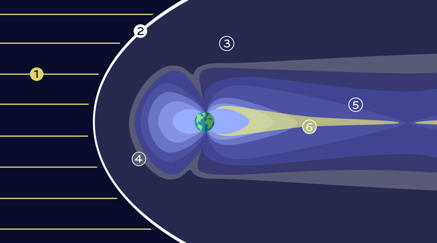
Figure 1: The structure of Earth’s magnetosphere: Earth’s magnetosphere is shaped by the pressure of the solar wind (1) — a torrent of charged particles that our Sun ejects outwards to interplanetary space. The solar wind interacts with Earth’s internally generated magnetic field, which decelerates at the bow shock (2), forming a shock wave. The boundary region at which the pressure of the solar wind is equivalent to Earth’s compressed upstream magnetic field is called the magnetopause (4). This region is nearly impenetrable and is located between geosynchronous orbit and the orbit of the Moon. The boundary layer between the plasma bow shock and the magnetopause is the magnetosheath (3), a transitional region where the density of particles significantly reduces compared to the bow shock. The complex internal structure of the magnetosphere evolves depending on factors such as solar activity. The open magnetic field lines connect to Earth’s polar caps where energetic electrons or protons contribute to aurorae. The magnetic field lines carried by the solar wind sweep in to the magnetotail (5), the teardrop shaped tail of the illustrated magnetosphere. Within the magnetotail, a dense plasma sheet (6) separates the magnetotail’s North and South lobes near the equatorial plane. The APIS mission would investigate both the magnetotail and the Sun-ward magnetosphere, with a particular focus on radio tomography in the magnetotail (5).

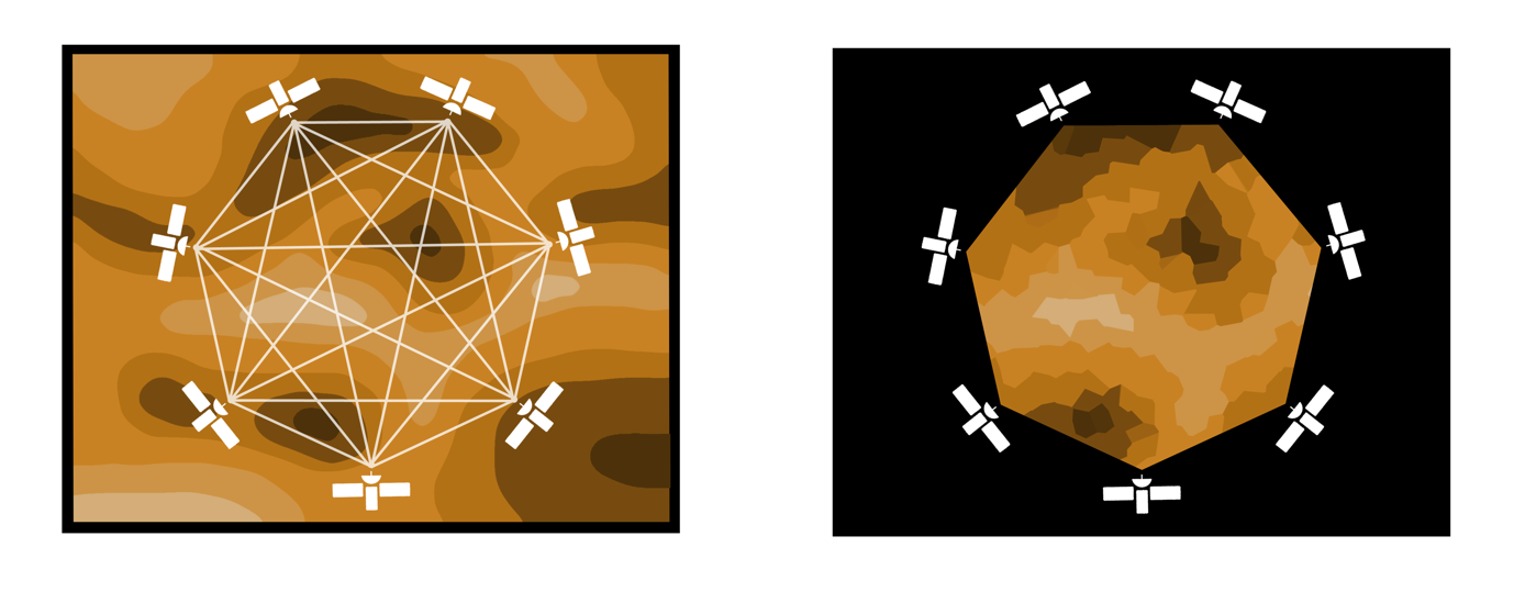
Figure 2: An illustration of tomography: Tomography is the process of imaging using penetrating waves, which are transmitted along the line of sight between nodes through the region of interest. In this illustration, the nodes are satellites and the waves are under consideration are in the radio spectrum. On the left, the image shows the spatial distribution of the plasma and the radio tomography links between the satellites. On the right, the image shows the tomographic reconstruction of the density field within the measured region is illustrated.

1.1 Motivation

Despite occurring on our astrophysical doorstep, some key physical processes connecting the solar wind and the magnetosphere remain poorly understood [1], motivating a steady stream of ongoing research. Understanding the magnetosphere is not only scientifically interesting, but also vital for today’s technologically dependent society. Energy transferred from the solar wind to the magnetosphere triggers electromagnetic storms on Earth, knocking out power grids and infrastructure such as communication networks, navigation, and transport. The effects of these geomagnetic storms on spacecraft can be disastrous [6]. Note, a better understanding and more detailed modeling can help us prepare and possibly prevent any catastrophic situations directly impacting human life. Given these practical and scientific motivations, understanding magnetospheric interactions and processes has been a driving requirement for decades of space science missions. There has been a plethora of studies and missions in the past to measure and study a variety of processes in our magnetosphere. However, despite the numerous heliophysics missions that have flown, plasma turbulence and the formation of plasma structures are still elusive and can only be understood with large-scale multi-point measurements. To achieve this goal, we propose the APIS mission (Applications and Potentials of Intelligent Swarms for magnetospheric studies) — a swarm of 40 autonomous CubeSats in two highly-elliptical orbits around the Earth, which perform radio tomography in the magnetotail at 8–12 Earth Radii ($R_{E}$) downstream, and the subsolar magnetosphere at 8–12 $R_{E}$ upstream. These maps will be made at both low-resolutions (at 0.5 $R_{E}$, 5 seconds cadence) and high-resolutions (at 0.025 $R_{E}$, 2 seconds cadence).

1.2 Outline

We begin our study with an overview of previous missions and case studies in Section 2, followed by listing the key science drivers for the APIS mission concept in Section 3. The detailed mission design and mission operations are presented in Section 4 and Section 5 respectively. The APIS satellites will comprise various science payloads, which are described in Section 6. Navigation, communication, on-board processing and power are critical aspects of the APIS swarm, which are addressed in Section 7, Section 8, Section 9 and Section 10 respectively. We present the APIS satellite configuration, summarize our findings, and present directions towards future work in Section 11.

2 Overview of missions and studies

2.1 Previous missions

In the past decades, more than 20 science missions have flown with the aim of investigating Earth’s magnetosphere, and many more mission proposals exist on paper. After decades of single-point measurements, multi-point imaging of the magnetosphere is pivotal to the upcoming heliophysics missions. These missions are more realizable given the rise in efficient small satellite architectures designs [7], the growing market in cubesat commercial vendors [8, 9] and a demand for various Earth observation missions [10]. In general, the space industry is witnessing a major disruption guided by innovation and determination to take bold risks [11].

One notable mission that has gathered distributed in-situ measurements is NASA’s ongoing mission, THEMIS [12]. Launched in 2007, the mission originally comprised of five satellites (each weighing 134 kg) in the magnetotail, and has provided over 12 years of data collection to date. The payload addresses the science goal of investigating substorms — magnetic phenomena that release energy and intensify aurorae. Another mission capable of collecting three-dimensional information on Earth’s magnetic environment and its interaction with the solar wind is ESA’s Cluster mission, which was launched in 2000 and is still operational. The four Cluster satellites flying in a tetrahedral formation probe the interactions of electrons and waves in Earth’s magnetic environment [13].

A relevant upcoming CubeSat mission is NASA’s CubeSat for Solar Particles (CuSP), which is designed to study solar particles in a three-month mission and to act as a pathfinder for a network of “Space Weather Stations”. The mission is planned to launch with the Space Launch System in 2021 and consists of a single $30\times 20\times 10$ cm CubeSat in a Sun-pointing, trans-Lunar, heliocentric orbit at 1 AU. On a larger scale, NASA’s Magnetospheric Multiscale (MMS) mission provides unprecedented high‐time resolution multi-point particle and field measurements [14]. Launched in 2015, MMS has a highly eccentric orbit and operates in Earth’s magnetosphere using four identical spacecraft flying in a tetrahedral formation. MMS researches the microphysics of magnetic reconnection, energetic particle acceleration, and turbulence – processes that occur in astrophysical plasmas. Additionally, a group of micro-satellites performed simultaneous multi-point measurements of Earth’s magnetic field as part of NASA’s ST5 (Space Technology 5). This 90-day mission mission flew in 2006 and tested 10 new technologies to pave the way for future multi-satellite missions such as MMS and THEMIS. Furthermore, ST5 contributed to an early understanding of the magnetosphere’s dynamic nature [15]. In recent years, the growing capabilities of small satellites have also led to a variety of innovative distributed heliophysics missions being proposed, developed, and funded [16, 17]. These missions leverage low launch costs and off-the-shelf hardware to offer scientific returns at a lower cost than traditional monolithic satellites [18]. However, in comparison to APIS, these missions typically comprise of either a single CubeSat or a handful of small satellites in a constellation [19, 20, 21, 22, 23, 24, 25].

2.2 Case studies

The science community has recognized for decades the need for satellites to make simultaneous, distributed heliophysics measurements. The distributed architecture of swarm satellites lends itself to high spatio-temporal range measurements [26], making it a promising architecture for such distributed measurement missions. Two case studies of proposed magnetic constellations provide insights on how the APIS swarm will perform a next generation heliophysics mission. The case study missions are NASA’s MagCon and MagCat, both of which were designed to probe Earth’s plasmasheet and magnetotail. NASA planned these missions to determine how the magnetosphere stores, processes, and releases energy in the magnetotail and accelerates particles to the inner radiation belts. The secondary scientific objective of the mission was to study how Earth’s magnetosphere responds to variable solar wind and how this influences the magnetopause, the boundary between the solar wind and Earth’s magnetic field. However, neither mission proceeded further than a concept due to budget constraints.

The Magnetospheric Constellation (MagCon): The proposed Magnetospheric Constellation mission was designed to perform distributed in-situ measurements of the magnetic field, plasma, and particles in such a way as to “revolutionize our understanding of the magnetospheric response to dynamic solar wind input and the linkages across systems” [27]. The mission concept was a constellation of up to 36 small satellites weighing 30 kg each with a typical spacing of 1–2 $R_{E}$ (Earth Radii), using orbits with perigees in the 7–8 $R_{E}$ range and apogees dispersed uniformly up to 25 $R_{E}$ [28]. Each spacecraft was designed with a boom-mounted magnetometer and a three-dimensional plasma analyzer to measure Earth’s magnetic field. A simple energetic ion-electron particle telescope was also included to analyse charged particle energization, loss, and transport throughout the heliosphere.

The Magnetospheric Constellation and Tomography (MagCat): The Magnetospheric Constellation and Tomography mission was designed to provide the first global images of the magnetosphere [29]. The mission was designed to examine plasma plumes in the magnetosphere, acquire reconstructed images of plasma density and turbulence using radio tomography, and measure three-dimensional ion and electron distributions. Tomography, that create maps of plasma density [30], is a key facet of the APIS mission.

3 Science drivers for APIS

The aforementioned missions and studies have significantly improved our understanding of small-scale physical processes in the magnetosphere, such as magnetic reconnection and plasma currents [31]. Despite the numerous heliophysics missions that have flown, plasma turbulence and the formation of plasma structures are still elusive and can only be understood with large-scale multi-point measurements [28, 32]. In 2004, NASA stated that MagCon’s database of dispersed measurements would allow us to “emerge from a long and frustrating hiatus” [33].

3.1 Motivation

The APIS mission would use a suite of instruments to bridge this gap by providing large-scale maps of plasma density and turbulence in the magnetotail — a need that was identified as early as 2000 [34]. The swarm architecture will allow the temporal and spatial resolution of the tomographic maps to vary over the mission. By providing these high-resolution maps, the APIS mission will address two of the four key science goals set out in the 2013 decadal survey on heliophysics [28]. The baseline tomography measurements meet the spatial resolution (0.5 $R_{E}$), and cadence (15 seconds) targets set out by the decadal survey, and the high-resolution operational modes comfortably exceed both of these targets. Based on the decadal survey and past, current, and future heliophysics missions, the APIS mission has two main scientific goals:

• Goal 1: Discover and Characterize Fundamental Plasma Processes in the Magnetosphere. The APIS mission shall measure the plasma flows and turbulence in the magnetotail using radio tomography and in-situ measurements. The use of a swarm architecture to produce high-resolution, small-scale tomographic maps, as well as large-scale observations will help explain key plasma processes that occur, not only in the magnetosphere, but also in magnetized plasmas across the universe [1]. These processes, such as turbulence in a magnetized plasma, require multi-scale multi-point measurements to be fully understood [32].

• Goal 2: Determine the Dynamics and Coupling of Earth’s Magnetosphere and the Response to Solar Inputs. The operational architecture of the APIS mission shall allow simultaneous plasma density measurements of both the magnetotail and the Sun-facing magnetosphere. The data provided by the APIS mission will uncover relationships between plasma density between different parts of the magnetosphere. Our orbital design would allow for detailed multi-plane measurements of plasma density in the magnetotail, providing long-awaited data to the heliophysics community at unprecedented spatial and temporal resolutions [34]. This data will provide an insight into the plasma dynamics of the magnetosphere in response to solar variation.

3.2 Regions of interest

The APIS mission will provide measurements in two initial regions of interest by launching two groups of swarm satellites. The two regions of interests will be in, (a) A near-equatorial orbit in the magnetotail, and (b) A polar orbit that sweeps through the magnetotail and the Sun-ward magnetosphere, over the course of one year. The region of interest for both equatorial and polar obits is 8–12 $R_{E}$ from Earth, where a host of scientifically interesting processes occur. After creating large-scale tomographic maps, the satellite swarm will then move on to the second phase of science operations and produce high-resolution maps of selected areas within the magnetotail.

The Magnetotail: One group of satellite swarms will be placed in a highly eccentric polar orbit, travelling through the magnetotail — the teardrop shaped tail of the magnetosphere streaming away from the Sun shown in Figure 1. Our region of interest is $8$–$12$ $R_{E}$, where key physical processes such as magnetospheric instabilities, plasma flows, morphological changes associated with geomagnetic storms, and turbulence occur [34, 31, 32]. Thus, this region has been intensely studied by previous missions, although at smaller spatial scales than we propose. Initial science observations will provide the big-picture data required to understand the region and the processes happening in this region. The high-resolution follow-up observations will then study these processes in more detail.

Polar plane: A secondary plane of the APIS mission swarm satellites will orbit on the same scale ($8$–$12$ $R_{E}$), nearly perpendicular to the first plane. This plane will sweep through the magnetotail and the Sunward magnetosphere over the course of a year. While in the magnetotail, the group of satellites in the polar plane will be able to enhance downstream measurements by increasing the region of focus. While in the sub-solar magnetosphere, the swarm satellites will be able to measure Sun-side dynamics. The measurements of plasma densities both up- and down-stream of Earth will uncover couplings and dynamics in Earth’s magnetosphere.

3.3 Science measurements

It is currently not possible to directly image the large-scale plasma structure in the magnetotail, as in-situ measurements require an extremely high number of satellites to achieve the desired resolution. Therefore, we propose to use radio tomography to reconstruct the spatial distribution of plasma. Tomography is the process of imaging with the use of penetrating radio waves. The radio waves are transmitted along many intersecting lines of sight through a region of interest. The density integral along each of these lines is derived from the delay in transmission. With many of these line integrals, an estimate of the density map of the region can be produced, as shown in Figure 2. Tomographic methods are well-developed for medical imaging, with examples including Computed Tomography (CT) scanning and medical ultrasound. Thus, the APIS mission will use radio tomography to create estimates of the plasma density in the magnetotail. Radio signals will be transmitted between the satellites and the time delay of each signal will be measured. The time delay of the signals is directly related to the total plasma density along the line-of-sight, and a map of the plasma density can then be reconstructed by mathematically combining the line-of-sight density measurements.

The study of the magnetosphere using spacecraft has been proposed [34] and tested [30]. Outside the magnetosphere, International Sun-Earth Explorers 1 and 2 have demonstrated the ability to derive the electron density in the solar wind through radio wave propagation [35]. With measurements between multiple spacecraft, the APIS mission will be capable of investigating the large-scale plasma density structure.

3.4 Science requirements

The primary region of interest for the mission is the magnetotail, in the range of 8–12 $R_{E}$ from Earth, and the desired resolution of the tomographic reconstruction is 0.5 $R_{E}$. Given the desired resolution of the resultant tomographic image $R_{S}$, and the effective diameter of the area of interest $d$, the approximate number of linear integrations required is: $N>\pi d/R_{S}$. The orbital characteristics and the number of spacecraft must meet this driving science requirement.

The radio tomography used by APIS relies on the propagation delay of radio waves within the plasma. The satellites of the APIS mission would use two steps to measure the characteristic delay along the line-of-sight. The first step is the differential phase measurement [36], which requires two coherent radio signals with different frequencies. The phase velocity of the radio signal in the plasma depends on the frequency and the plasma density. The phase of a probing frequency is compared to the phase of a reference frequency transmitted through the plasma, and the resulting phase delay depends on the plasma density as follows:

$$\Delta\phi_{1}=\left(\frac{\omega_{1}e^{2}}{2\varepsilon_{0}m_{e}c}\right)\left(\frac{1}{\omega_{1}^{2}}-\frac{1}{\omega_{ref}^{2}}\right)\int ndL$$ (1)

where, $\omega_{1}$ is the probing frequency, $e$ is the electron charge, $\varepsilon_{0}$ is the vacuum permittivity, $m_{e}$ is the electron mass, $\omega_{ref}$ is the reference frequency, and $n$ is the total electron content [34]. If the phase delay is greater than $2\pi$, then the second step of delay measurement must be employed. The group delay resolves the phase delay that is proportional to total electron content:

$$\Delta t_{g}\cong-\frac{e^{2}}{2\varepsilon_{0}m_{e}c}\left(\frac{1}{\omega_{1}^{2}}-\frac{1}{\omega_{ref}^{2}}\right)\int ndL$$ (2)

where $\int ndL$ is directly proportional to the total electron content [37]. By combining the methods of differential phase delay (1) and group delay (2), we can derive the total electron content. A long-wavelength probing frequency is desired because both types of delay are inversely proportional to frequency. In-situ measurements of the magnetic field and the plasma density are required to interpret the tomography measurements correctly. The scientific measurements must also be correlated with time and position data to produce a complete picture of the magnetotail environment. Tables 1 and 2 encapsulate the scientific motivation and requirements of the APIS mission, as well as the measurement accuracies required. These requirements are based on the decadal survey and previously proposed missions, which can be feasibly achieved with current technology [34, 31, 25, 28].

Table 1: Science requirements for the APIS mission, where Extended, Baseline and Threshold denote the NASA terminologies for best case, baseline and minimum requirements respectively.

Requirement	Extended	Baseline	Threshold
Large-Scale Radio Tomography Phase	Multi-plane tomographic maps of the magnetotail 8–12 $R_{E}$ downstream, and the subsolar magnetosphere at 8–12 $R_{E}$ upstream with 0.5 $R_{E}$ resolution. All measurements at 5 seconds cadence.	Tomographic maps of the magnetotail 8–12 $R_{E}$ downstream, and the subsolar magnetosphere at 8–12 $R_{E}$ upstream with 0.5 $R_{E}$ resolution. All measurements at 10 seconds cadence.	Tomographic maps of the magnetotail 8-12 $R_{E}$ downstream with 0.5 $R_{E}$ resolution. All measurements at 15 seconds cadence.
Fine-Scale Radio Tomography Phase	High-resolution tomographic maps of small regions of the magnetotail 8–12 $R_{E}$ downstream at 0.025 $R_{E}$ spatial resolution. Measurements at 2 seconds cadence for short bursts.	High-resolution tomographic maps of small regions of the magnetotail 8–12 $R_{E}$ downstream at 0.05 $R_{E}$ spatial resolution. Measurements at 3 seconds cadence for short bursts.	High-resolution tomographic maps of small regions of the magnetotail 8–12 $R_{E}$ downstream at 0.1 $R_{E}$ spatial resolution. Measurements at 5 seconds cadence for short bursts.
In-situ measurements to anchor tomography	Measurements of magnetic field, electric field, plasma energy distribution, plasma density; at 2 seconds cadence.	Measurements of magnetic field, plasma energy distribution, and density; at 3 seconds cadence.	Measurements of magnetic field and plasma density at 5 seconds cadence.
Positional Knowledge	0.01 $R_{E}$ (63.71 km)	0.01 $R_{E}$ (63.71 km)	0.01 $R_{E}$ (63.71 km)
Time Knowledge	0.01 microseconds	0.01 microseconds	0.01 microseconds
Duration of Science Observations	1 Solar cycle (11 years)	2 years	4 months

Table 2: Science measurement requirements of the APIS mission (all measurements will have a variable cadence of up to 2 seconds)

Measurement	Range	Resolution
Radio Tomography Plasma Density	0.05–150 cm3	2 % error acceptable
Magnetic Field	0–2000 nT	0.025 nT
Plasma Particle Energy	1–5 MeV	15-20%
In-situ plasma density	0.05–150 cm3	2% error acceptable

3.5 The APIS mission

The APIS mission will address key physical processes in the magnetosphere, including: how plasma enters the magnetosphere; the formation and dynamics of the plasma sheet; the formation of plasma structures in response to solar wind variability; and turbulence in a magnetized plasma [28]. By exploiting the swarm architecture, the APIS mission will provide large-scale, high-resolution tomographic maps that exceed the targets set out in the 2013 decadal survey on heliophysics [28]. The novel scientific feature of the APIS mission is the swarm-enabled ability to vary the spatial and temporal resolution of the tomography measurements, which will provide the precise data needed to understand key heliophysics processes. The APIS mission requirements - as discussed at length in this article - are summarized in Table 3, and are derived from the science requirements as described in Table 1 and Table 2.

Table 3: APIS mission overview

Mission requirements
Launch capability	40 spacecrafts in 2 elliptical orbits
Mission duration	4 months science phase
Orbital requirement	8–14 $R_{E}$, one polar and one near-equatorial plane
Spacecraft requirements
Attitude stabilization	3-axis stabilized
Mass	21.8 kilogram  (see Table 14)
Power	63.2 watts (see Table 11)
ISL Data rate	$\geq$ 100 kbit/sec
Pointing	$\leq 5^{\circ}$ accuracy, $\leq 2^{\circ}$ knowledge

The APIS mission architecture comprises of a homogeneous satellite swarm spread over two orbits, polar and near-equatorial, as illustrated in Figure 3, using the Systems Tool Kit (STK). The swarm satellites will exhibit emergent behavior through cooperation in order to achieve tomography measurements, reference-free calibration of instruments, navigation, and data handling. The presented orbits meet a set of requirements, derived from the science objectives. Table 4 shows the mission orbital parameters, where the Right Ascension of the Ascending Node (RAAN) and the argument of perigee are excluded at this time, since the two will depend on the time and date of the launch.

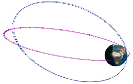
Figure 3: Mission Design: An illustration of the two orbits in the APIS mission — i.e., the Polar orbit (in blue), and the Near-Equatorial (in pink)

.

Table 4: Mission orbital parameters

Parameters	Value	Comments
Apogee	13 $R_{E}$ (altitude)	14 $R_{E}$ from the center of Earth in order to enclose the region of interest, defined in by the science objectives.
Perigee	500 km (altitude)	Higher than ISS orbit
Inclination	$\sim 0^{\circ}$ and $\sim 90^{\circ}$	One inertially locked in polar, other precesses
Number of satellites in each plane	20	Train formation, 18∘ of angular separation
Eccentric anomaly of the $\mathbf{n^{th}}$ satellite	$i\frac{360}{20}n^{\circ}$	18∘ of angular separation, $n$ is the satellite number (between 1 and 20)

Over the course of one orbit, the mission operations are subdivided into various phases as illustrated in Figure 4(a), which include the science phase and the ground operation phase. The green region indicates the ground link for the mission. Due to the highly eccentric orbit, each satellite will have a window of  $1$-$2$ hours per orbit for communication with the ground station. The satellites will distribute data amongst the swarm and queue the data in order of importance to the science mission for downlink. The sharing and queuing allows for an effective downlink window of up to 20 hours. The region between the perigee and 8 $R_{E}$ is dedicated for other functions, such as orbital maneuvering and attitude control.

The red region in Figure 4(a) indicates the science phase of the orbit, where the swarm performs tomography and plasma measurements. If one of the satellites recognizes an interesting physical phenomena, then the satellite needs to direct the rest of the swarm to take increased measurements through a consensus approach. At the apogee the satellites slow down due to orbital dynamics and the distance between them is reduced to enable better communication between the agents. Therefore, in addition to the science case, the inter-satellite links are also established during this phase, which is critical for swarm-related data processing. Furthermore, individual agents perform science logging preferentially during the ascending phase (agents moving from perigee to apogee), which ensures that inter-satellite data exchange occurs near apogee.

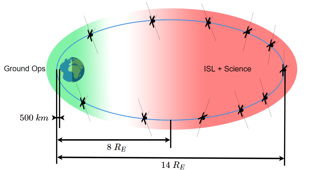
(a)

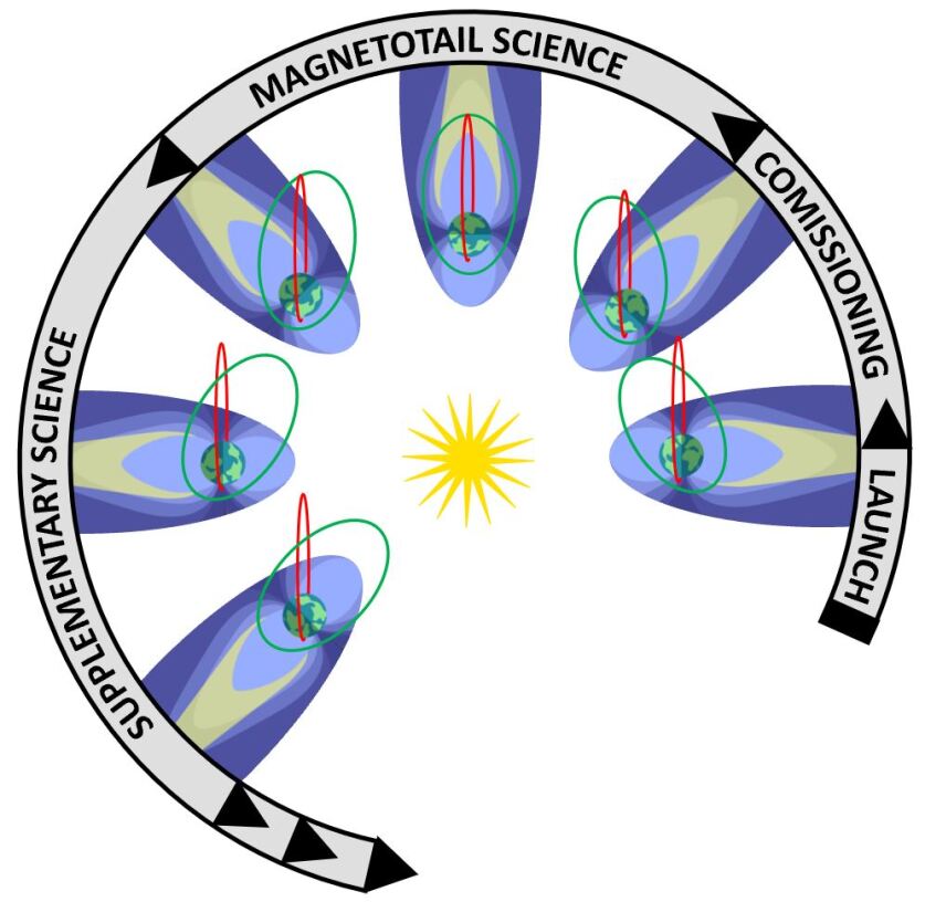
(b)

Figure 4: Illustration of the APIS mission operational phases and configurations: (a) The orbital configuration of the swarm over the course of the one-year mission is illustrated (b) The phases of the APIS mission are illustrated, over the course of an orbital period for each satellite in the swarm.

4 Mission design

The objective of the science mission is to map the plasma densities at the scale of $0.5~{}R_{E}$, for a region of interest from $8~{}R_{E}$ to $12~{}R_{E}$. To achieve our goal we have designed the swarm to fly in two orbits perpendicular to one another at inclinations of $90^{\circ}$ and approximately $0^{\circ}$, with an apogee radius of $14~{}R_{E}$, enclosing the magnetospheric area of interest. This configuration enables tomography in the magnetotail, as well as in the Sun-ward magnetosphere. In Figure 4(b) the orbital dynamics that occur during the first year of the mission are illustrated, and the mission phases timeline is described in Table 5.

Table 5: Mission Phases Timeline

Phase	Description	Mission Timeline	Duration
Launch	Launch into highly eccentric orbit	1st day	$<$1 day
Deployment and commissioning	Swarm agents are deployed at apogee into two possible inclinations (0∘ or 90∘), 20 agents per orbit. Subsystems and payloads are validated and calibrated.	1st day	3 weeks
Science Phase 1	Swarm agents cooperate to perform tomography and plasma property measurements in the magnetotail region.	3rd week	3.5 months
Science Phase 2	Cooperative tomography and plasma measurements in the Sun-ward magnetosphere region are performed on the equatorial orbit, and later on the polar orbit.	6th month	3 months
Science Phase 3	Reconfiguration of swarm agents is executed on both orbits to perform higher resolution tomography in a $2~{}R_{E}$ strip of the magnetotail region	1 year	4 months
Maintenance and Ground Operations	Desaturation of reaction wheels, charging downlink of scientific measurements prioritized by swarm agents, and data analysis.	All mission
End of life	Passivation of subsystems, natural orbit decay, comprehensive data analysis	Dependent on orbit decay

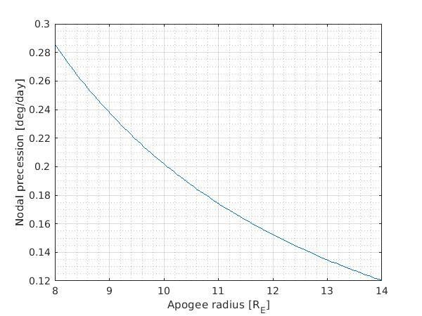
(a)

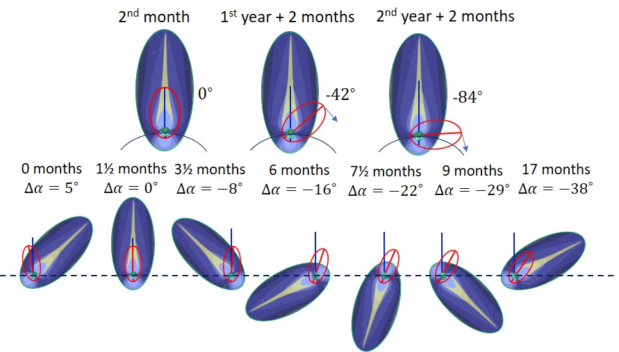
(b)

Figure 5: Variation of nodal precession against apogee: (a) The equatorial orbit used in the mission will experience nodal procession rates of 0.12^∘–0.29^∘ per day while the apogee radius is 8–14 $R_{E}$. (b) Precession of the equatorial orbit relative to the magnetotail.

4.1 Nodal precession of the Orbit

One of the main features of the mission orbit design is the differing nodal precession that occurs between the equatorial and polar orbits, causing the semi-major axis of both orbits to no longer be aligned. Orbital precession affects the orientation of the elliptic trajectory of spacecraft. Nodal precession is defined as the rotation of the orbital plane around the axis of the central body, Earth in our case. This phenomenon is caused by non-uniform mass distribution in the central body, and in a first approximation, the major contributor is the equatorial bulge of Earth that causes the planet to be an oblate spheroid with a larger diameter at the equator than at the poles. The relationship that relates the precession rate to the orbital elements is the following:

$$\omega_{p}=-\frac{3}{2}\frac{R_{E}^{2}}{(a(1-e^{2}))^{2}}J_{2}\omega\cos{(i)}$$ (3)

where, $a,e,\omega$ and $i$ define the orbit, $R_{E}$ is the equatorial Earth radius, and $J_{2}$ represents the perturbations due to the oblateness of the Earth. From the two orbits in the APIS mission, only the equatorial orbit is affected by nodal precession. The polar orbit, as characterized by an inclination of 90^∘, nullifies the precession due to the $cos(i)$ term in the equation given. While the satellites pass through the region of interest and the apogee radius remains between $8~{}R_{E}$ and $14~{}R_{E}$, where science measurements are to be performed, the experienced precession rates will range between $0.12^{\circ}$ and $0.29^{\circ}$ per day. Figure 5(a) illustrates how the regression rate varies while the orbit decays in relation to the phases, as illustrated in Figure 5(b).

4.2 Orbital maneuvers

The minimum science requirement is achieved in the course of the first 3–4 months into the mission, with tomography in the magnetotail. The mission then continues for an additional two months to perform measurements of the plasma density outside the tail. Following this timeframe, the extended mission will exploit the swarm ability to reconfigure and take new measurements. The objective of the new geometry is to perform higher resolution tomography, as the satellites sweep through the magnetotail in the next orbital pass about $12$ months into the mission, which is detailed in Table 5.

Reconfigurability: In the proposed scenario, five satellites from each orbit will perform a maneuver to change their apogee to $2~{}R_{E}$ lower than the reference orbit at $14~{}R_{E}$. The remaining $30$ satellites will stay in their original orbits. The maneuver will take approximately nine months, commencing outside the magentotail and terminating before the satellites sweep through the magnetotail again. Modifying the trajectory of the APIS satellites requires significant thrust due to the high energy of the orbit, as well as a regenerative propulsion system for the extended mission duration. To overcome this difficulty, we will use the electric propulsion system on each APIS satellite, which can operate over long periods of time (see Section 7.4). The atmospheric drag experienced during flight close to perigee can also be utilized. One of the major trade-offs to be considered is the effect of different orbital periods between Group 1 (in the near-equatorial orbit) and Group 2 (in the polar orbit). In Figure 6, the apogee alignment between the two groups is presented, as the orbit decays and the period changes. The two groups are aligned when they reach apogee within one hour of one another.

In a first approximation, the electric propulsion system will enable an apogee of $30$ km per orbit when used to reduce the velocity in perigee. Attitude control orients the satellites to maximize the satellite surface area exposed to the thin atmosphere. The minimum surface area, used to maintain the $15$ satellites in the reference orbit, is $0.06$ m². The maximum possible area exposing the solar panels is $0.52$ m², which induces a drag of more than eight times greater than otherwise. Indicatively, the orbit decay, induced by drag on the five satellites moving to the lower orbit, is $20$ km per orbit at a perigee altitude of $500$ km. A first estimate of the total decay rate induced combining both electric propulsion and drag is in the order of 50 km per orbit.

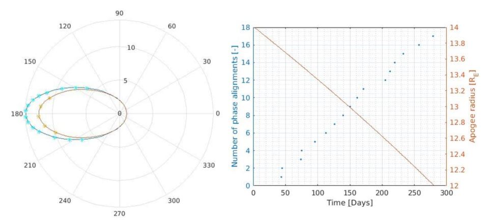
Figure 6: Effect of differing orbital periods between groups 1 and 2: Frequency of apogee alignment between a fixed reference orbit and a reconfigured high resolution orbit is presented.

The swarm is expected to implement emergent behavior to achieve collaboration between the two orbital groups, thereby improving the potential science return. This emergent behavior arises from simple rules followed by the satellites, without the need for a centralized coordination, and thus enabling the APIS swarm to collectively behave as a single entity. The desired behavior is to modify the altitudes of both orbits, maximizing the frequency of apogee alignment. This modification will require each satellite to plan the desired attitude at perigee to modulate both the amount of drag experienced and the thrust generated due to turning the propulsion system on and off.

4.3 End of mission

As the swarm decays below the region of interest of $8~{}R_{E}$, the APIS mission enters the final stage, and no more research is viable. Rapid decay will help minimize the number of spacecraft in orbit. The orbit apogee will decay to a $500$ km, placing teh satellites into a circular orbit due to the effects of atmospheric drag on the satellites. Once in the circular orbit, the final resources from the propulsion system will be used to lower the perigee and apogee below the altitude of the ISS. Then the satellites will orbit at the maximum drag attitude orientation while passing through perigee. This procedure will allow for rapid de-orbit, reducing possible intersection with the ISS orbit at lower altitudes.

5 Mission operations

Over the course of the full APIS mission, the satellite swarm will undergo key operational phases. In this section we present an overview of the four mission phases: launch, deployment and commissioning, science, and decommissioning.

5.1 Launch phase

Our proposed orbit design outlines a scenario of 40 spacecraft distributed over two orbital planes. The difference in inclination between the two planes is 90^∘. In addition to mass, an important requirement for the launcher is its fairing volume. The total volume to be occupied by the APIS satellites is 0.48 m³. A single launcher will first inject the whole swarm into a highly eccentric equatorial orbit. Then, once at apogee, a kick-stage will provide enough $\Delta v$ to change the orbital plane for 20 of the 40 satellites from equatorial to polar. Performing the maneuver at apogee will optimize the use of propellant mass. The following equation provides the $\Delta v$ required:

$$\Delta v=2v_{a}\sin{\bigg{(}\frac{\Delta i}{2}\bigg{)}}$$ (4)

where $v_{a}$ is the velocity at apogee, and $i$ is the inclination of the orbital plane. For the APIS mission the final stage will impart a $\Delta v$ of $1.13$ km/s to a payload mass of $520$ kg. The SpaceX Falcon 9 is a launcher that best meets the requirements of the mission, considering both cost and capabilities. The block 5 iteration of the rocket is capable of positioning 8300 kg in Geostationary Transfer Orbit (GTO) [38]. Thus, it would be possible for the APIS satellites to share the launcher with other missions, therefore reducing the cost. Placing the apogee from the geostationary belt to the required orbit will require a further $\Delta v$ of $820$ m/s.

5.2 Deployment and Commissioning

All satellites will be attached to an EELV Secondary Payload Adapter (ESPA) ring, which is an adapter for launching secondary payloads on orbital launch vehicles and has become a de facto standard for various spaceflight missions [39, 40, 41]. The commissioning phase is automated, and each swarm satellite tests their payload and bus systems. The satellites transmit any anomalies to the ground for further investigation. Due to the swarm capability, the swarm group in one orbital plane can start its science phase without the need to wait for the swarm group in the second plane. Once all satellites are deployed and commissioned in both orbital planes, the science phase will generate results at a significantly higher rate.

5.3 Science phase

The majority of the mission’s lifetime is the science phase. The orbital design allows the swarm satellites to be in the magnetospheric region of interest by use of orbit precession. The science phase (at an altitude above 50000 km) lasts for 27 hours per orbit. Tomography techniques require a minimum number of lines to reach the necessary spatial resolution. The swarm will achieve this minimum threshold by performing tomography measurements when close to the apogee area, where the satellites cluster together at a range of $2~{}R_{E}$ to $8~{}R_{E}$ separation distance due to orbital dynamics. The transmissions will synchronize, using the Code-Division Multiple Access (CDMA) protocol, which leads to the notable swarm behavior. An illustration of these Inter-satellite Links (ISLs) within the swarm is shown in Figure 7(a).

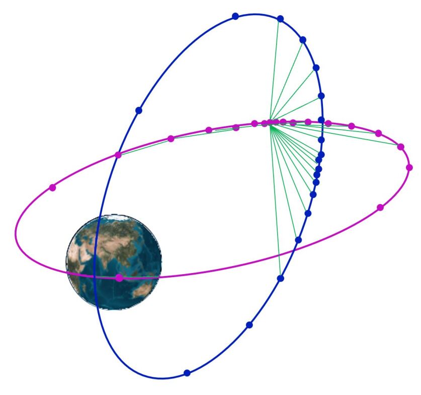
(a)

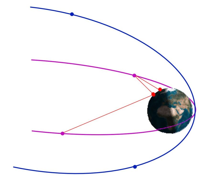
(b)

Figure 7: (a) Inter-Satellite Link (ISL): An illustration of APIS ISLs within the swarm in the APIS mission. (b) Downlink: Swarm satellites can communicate with ground stations while in the equatorial orbit. Red lines indicate ground link communication with satellites.

Each satellite will also perform in-situ measurements of the particle distribution and plasma properties for the tomography data processing. During the 4-month science phase, the satellites will perform 1000 measurement sequences. After each satellite stores its data, the swarm will perform autonomous measurement prioritization based on information theory, which maximizes the scientific return of the swarm. While clustered at apogee, ISL communications are enabled between neighbouring satellites for measurement sharing, data sorting, and autonomous decision-making on measurements to be kept in the collective swarm memory for maximizing the scientific data quality.

6 Science payloads

All the satellites in the APIS mission have a payload suite comprising of multiple science payloads, including the radio tomography system, and various in-situ measurement systems. In addition, all APIS satellites will employ on-board Radio-Frequency Interference Mitigation (RFIM) techniques and sensor calibration to ensure the veracity of the recorded science data.

6.1 Radio tomography

Large-scale in-situ measurements of the entire field of interest would require a significant number of satellites, however, with our proposed design, we use radio tomography in order to estimate the plasma density map. In radio tomography imaging, each satellite transmits a coherently phased pair of discrete radio signals, which in turn is received by all satellites. The measured phase difference between the signals, integrated along the ray path, yields the Total Electron Content (TEC). For a network of 20 satellites, with a maximum distance separation of 8 $R_{E}$, each inter-satellite transmission and reception takes up to 0.3 seconds, and the entire tomographic cycle takes up to 3 seconds [34]. The choice of the frequency pair — i.e., the probing and reference frequencies — plays a vital role in the mission design. For example, in the MagCat mission (see Section 2.2), the probing and reference frequencies were of 1 MHz and 3 MHz — i.e., the third harmonic was used [34]. To transmit and receive at these selected wavelengths, a half-wave dipole antenna of approximately 50 m is required, which increases both the mass and power budget of the small satellites.

To overcome power and mass limitations, the APIS mission plans to use 10 MHz and 30 MHz, as the probing and reference frequencies, respectively. The necessary antenna lengths at these wavelengths is approximately 15 m, which is suitable for the small satellites of the mission. Radio measurements at these selected frequencies can become significantly corrupted by man-made interference [34]. Thus, the APIS mission employs the on-board RFIM technique to resolve this issue. The dual polarized radio signals received by each satellite is to be pre-processed by the Signal Conditioning Unit (SCU), digitized by the Analog to Digital Converter (ADC), and filtered by a Poly-phase Filter Bank (PFB). Finally, the man-made interference is removed by the RFIM block, as illustrated in Figure 8.

The swarm satellites are to deploy two 7.5 m dipole antennas, which will unfurl in measuring tape fashion. The boom material is a carbon fiber reinforced polymer, while the design is a combination of two arms in the form of ‘C’-sections with one inside the other to reduce volume. The boom will also act as an insulator, and thus, will be wrapped with aluminized Kapton or a similar coating to control electrostatic discharge [42].

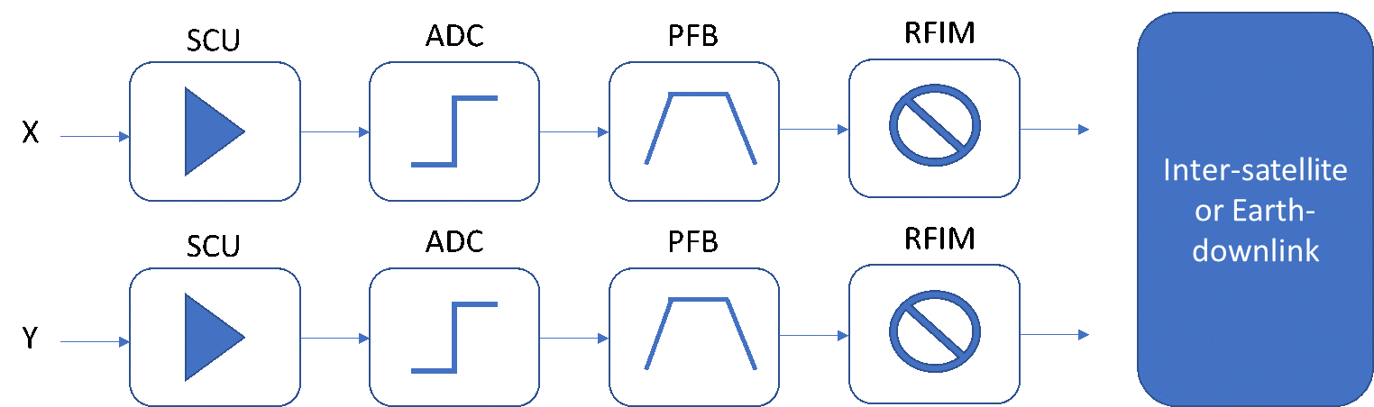
Figure 8: Signal processing for RFI mitigation: The block diagram shows a breakdown of the signal processing for radio tomography within a single APIS satellite.

6.2 In-situ measurements

In addition to the radio tomography payload, there are $3$ additional payloads on-board the satellites for in-situ measurements.

• Super-thermal Ion Spectrograph: The super-thermal ion spectrograph is based on the electrostatic analyzer payload proposed for the CuSP mission [25]. The payload occupies a volume of $1.5$U. The payload provides a measure of the energy spectra and the peak intensities of the incident particles, thereby providing in-situ measurements of the magnetospheric plasma.

• Miniaturized Electron and Ion Telescope: This payload is based on a flight-proven payload flown on the Compact Radiation Belt Explorer mission in 2018. Our payload will be shielded with tungsten and aluminum, which increases the mass but is necessary to reduce the background noise caused by scattering. The APIS mission miniaturized electron and ion telescope instrument contains a stack of SSDs to image the electron and ion paths. Similar payloads have been flown on-board the ISS [43].

• Vector Helium Magnetometer: Vector helium magnetometers have been used in previous missions to measure magnetic fields in various environments. These magnetometers measure the optical properties of helium, which change in an applied magnetic field. Recent and upcoming missions have miniaturized this instrument, and it is now adapted for CubeSat missions like CuSP [25].

6.3 Calibration

Calibration is a key challenge for these on-board detectors, especially in long-term multi-year missions. Conventionally, operators on Earth correct the errors accrued by the detectors over time via telemetry. As an alternative, the swarm satellites can communicate with each other to employ relative or reference-free calibration, to eliminate the detector errors such as offsets and gain [44]. Since the signal subspace is unknown, the nodes can employ blind calibration [45], which would involve a training phase during the initial deployment of the antennas. Distributed calibration algorithms will be used to ensure the APIS satellite swarm could collectively alleviate their on-board detector errors [46].

7 Navigation

One of the key challenges for the APIS swarm lies in navigation, i.e., in ensuring accurate position, time and orientation estimation and control. A single satellite in the APIS mission has the visibility of GNSS satellites only for a few hours per orbit. In the absence of GNSS, all the satellites rely on their respective on-board Attitude Determination and Control Systems (ADCS), and the two-way communication with the other satellites in the swarms using Inter-satellite Links (ISLs). In this section, we discuss the clocks and time synchronization, the ADCS system on-board the satellite, and localization strategies with and without GNSS. All the data processing pertaining to the ADCS system will be done by the OBC (Section 9). In addition to the space and time estimation of each satellite, the propulsion system on-board each satellite used for orbital correction is also presented.

7.1 Clocks and Time synchronization

The on-board clocks of the satellite swarm in the APIS mission will need to be synchronized for navigation, communication, and addressing the science mission [47]. The radio tomography requires accurate transmission and reception at frequencies of $10$ MHz and $30$ MHz, which is identical to the wavelengths used in interferometry in ultra-long wavelength radio astronomy [48]. The intrinsic stochastic noise on the clock is typically measured in Allan deviation over a coherence time period [49]. The Allan deviation requirements for clocks at these wavelengths are typically in the range of $10^{10}$–$10^{13}$, which is typically achieved by oven-controlled crystal oscillators or Rubidium standard clocks [49]. To ensure programmable output frequencies, we propose the use of VCXO Si570, which additionally offers a low-jitter clock output for the range of $0.01$–$1.4$ GHz [50]. The in-depth study of available clocks is beyond the scope of this project, and is excluded for this reason.

A solution is to align all the on-board clocks within the swarm, is clock synchronization based on time-stamping. Given a time-varying mobile network of satellite swarms, the first-order clock errors, i.e. clock offset and clock drift, can be estimated jointly along with the time-varying distances between the satellites. The satellites will employ two-way ranging to collect the transmitted and received time-stamps. Typically, these measurements are input parameters to optimization algorithms for estimating the unknown clock and distance parameters. In [51], a constrained least squares algorithm is proposed to estimate these unknown parameters using only time-stamp measurements between the satellites. Furthermore, such algorithms can achieve time synchronization within the network, as long as each satellite has at least one communication link with any other satellite in the network. In addition, a reference for the clock is chosen arbitrarily in the network, and alternatively data-driven references are chosen from the network [51]. The achievable timing accuracy using these algorithms is directly proportional to the bandwidth of communication (i.e. number of time-stamps exchanged), and the SNR of the signals.

7.2 Attitude Determination and Control System

The Attitude Determination and Control System (ADCS) in the APIS satellites will comprise of various sensors and actuators to estimate and control the satellite attitude [52]. The chosen components in the ADCS system are COTS components, and have validated flight heritage.

• Reaction wheels: There are various micro-reaction wheels available on the market, which provide a small torque change, and create fine rotations, weighing $<300$ g [53]. A favourable choice is the RWP015 from Blue Canyon Tech, which weighs as low as 130 grams and has a design life of more than five years, making it suitable for the APIS mission [54]. The APIS mission will use the 4-wheel tetrahedron configuration such that in the event of wheel failure the mission can still continue without interruption [52].

• Magnetic torquers: In addition to the reaction wheels, magnetic torquers are used for attitude control, detumbling, and stabilization using the Earth’s magnetic field. The torquers consist of electromagnetic circuits without moving parts, making magnetic torquers reliable and resilient to radiation effects in comparison to other devices with sensitive electronics [55]. For the APIS mission, we chose the ISISpace iMTQ Board, which is a PCB-based 3-axis magnetic actuation and control system for 12U CubeSats [56]. It weighs less than $196$ grams and is designed as a standalone detumbling system and can also be used with more advanced ADCS hardware, providing actuation of $0.2$ Am², with a magenetometer accuracy of $<3~{}\mu$T.

• Star Trackers: Star trackers are one of the most accurate sensors for satellite attitude estimation, as required during payload operation, Sun pointing, and for ground link communications. For the APIS mission, we chose a single NST component from Blue Canyon Tech, which offers an attitude resolution of $6$ arcseconds (cross boresight) with a Field of View (FOV) of $10^{\circ}\times 12^{\circ}$, and weighs as low as $350$ grams [57].

• Sun Sensors: In addition to Star trackers, APIS satellites will have Sun sensors on-board to provide orientation information. Sun Sensors are generally less accurate in comparison to star trackers but offer a larger FOV at typically lower costs. There will be four Sun sensors placed in the four selected corners or faces of the satellite body, which is sufficient to provide satellite orientation information with respect to the Sun. The APIS mission will use the two-axis sensor, NFS-NFSS-411, which weighs less than $35$ grams, and offers an accuracy of $0.1^{\circ}$ with a FOV of $140^{\circ}$ [58].

• Inertial Measurement Unit (IMU): IMUs combine accelerometers and gyroscopes, which provide acceleration and orientation information of the satellite, respectively. In particular, MEMS-based IMUs are lightweight and reliable, with longer mission life and offer a high Technology Readiness Level (TRL). There are numerous COTS MEMS-based IMUs available in the market — e.g., the Sensonor STIM377H, which is a tactical grade 3-axis IMU comprised of $3$ accurate MEMS gyros, $3$ high stability accelerometers and 3 inclinometers [59]. Each APIS satellite will have $4$ of these IMU units.

7.3 Relative localization

Huff et al. [60], present a method of obtaining accurate absolute and relative position estimates of a swarm of small unmanned aerial systems. In the APIS mission, each satellite will have full access to GNSS signals for only a few hours per orbit. GNSS for navigation will therefore be unsuitable for the extended mission duration. The swarm enables collective navigation –- i.e., the satellites’ relative position to each other can be constantly determined. Each APIS satellite will require a GNSS unit, an IMU, and an ISL. When available, GNSS signal measurements will be integrated with the estimated relative positions to determine the absolute position of the satellites. The APIS satellites will use a NovAtel OEM719 multi-frequency GNSS receiver, and the on-board firmware can be reconfigured to offer sub-metre to centimetre positioning, meeting the APIS science requirements [61].

For an immobile network, in the absence of a reference such as GNSS, the relative position of the satellites can be estimated using multi-dimensional scaling like algorithms [62]. Furthermore, [63] proposed a distributed relative position algorithm, which offers a solution to solve for the relative position of satellites cooperatively on a sphere domain. When the satellites are mobile, the relative kinematics (e.g., relative velocity and acceleration) need to be estimated by solving relative kinematics models [64]. A large consideration for the APIS team is distributed control for the swarm in terms of position and attitude. Path-planning feedback control for autonomous and distributed position control of satellite swarms will be implemented, using local sensor data to coordinate individual satellite tasks, with the assumption that each satellite is able to locally process 3D attitude and inter-satellite distances from the on-board sensors. Each satellite can evaluate, in real-time, the final target position based on the available sensor information, and safely navigate to the chosen position while avoiding collision with another satellite. This method of control uses low computational resources and autonomous position selection with safe acquisition [65], which suit the APIS mission.

7.4 Propulsion system

The propulsion system consists of thrusters mainly used for orbital corrections. The satellites in the APIS mission require in-orbit corrections, and therefore, an on-board propulsion system. Two popular solutions include the Pulsed Plasma Thruster (PPT) and the Micro Electrospray Propulsion (MEP). MEPs use the principle of electrostatic extraction and acceleration of ions. The propulsion system does not require gas-phase ionization, which is an advantage. The propellant is not pressurized since it flows through capillary action. The emission is controlled by modulating the voltage applied, which provides better safety in handling the spacecraft, and light weight spacecraft [66]. MEPs offer high system-level and power level efficiencies. However, there are severe system scalability issues, thus, making MEPs harder to use.

In constrast, PPTs are known for having a high specific impulse, consisting of low power electric thrusters for precise spacecraft control, and can be used for orbit maintenance [67]. The thruster uses electricity to vaporize the solid Teflon propellant to generate thrust. PPTs do not need a tank or feed system, are compact, low-cost, and consume less power in contrast to MEPs. The drawback of a PPT operation is that it may create disturbances in payload science measurements because of the possible mixing of propulsion plasma with magnetotail plasma. We can mitigate for this risk with strategic scheduling of propulsion use [68]. The APIS satellites will, therefore, use a variant of PPT called Filament Pulsed Plasma Thruster (FPPT), which uses a Polytetrafluoroethylene propellant [69]. Two propulsion systems will be placed aligned to the center of mass such that the system can be used for both linear and rotational movement. The thruster can also be used as a desaturating unit for the reaction wheels through the on-board computer (OBC).

Table 6: Comparison of various Antennas

Manufacturers	NanoAvionics	Endurosat	Anywaves	AAC-Clyde Space	Surrey
Website	n-avionecs.com	endurosat.com	anywaves.eu	aac-clyde.space	surreysatellite.com
Operating Frequency (MHz)	2400-2450	2400-2450	2025-2290	2200-2300	2000-250
Gain (dBi)	6	8.3	6.5	7	3
Circularly Polarized	Yes	Yes	Yes	Yes	Yes
Mass (g)	49	64	123	50	80
Dimension (l$\times$w$\times$h mm)	70 $\times$ 70 $\times$ 12	98 $\times$ 98 $\times$ 12	79.8 $\times$ 79.8 $\times$ 12.1	81.5 $\times$ 89 $\times$ 4.1	82 $\times$ 82 $\times$ 20

Table 7: Comparison of various Transceivers

Manufacturer	NanoAvionics	ECM	Spacecom	Skylabs
Website	n-avionecs.com	ecm-space.de	iq-spacecom.com	skylabs.si
Tx. Freq. (MHz)	2200-2290	2200-2290	2200-2290	2200-2300
Rx. Freq. (MHz)	2025-2110	2025-2110	2025-2110	2000-2100
Tx. Bit Rate	128-512 kbps	20 Mbps	20 Mbps	4 Mbps
Modulation	GMSK	QPSK, BPSK	BPSK, QPSK, 8PSK	OQPSK
Output Power (dBm)	30	27	30	30
Power Consumption (W)	5	12	13	5
Mass (g)	190	190	190	90
Dimension (l$\times$w$\times$h mm)	87 $\times$ 93 $\times$ 17	50 $\times$ 55 $\times$ 94	50 $\times$ 55 $\times$ 94	95 $\times$ 91 $\times$ 10

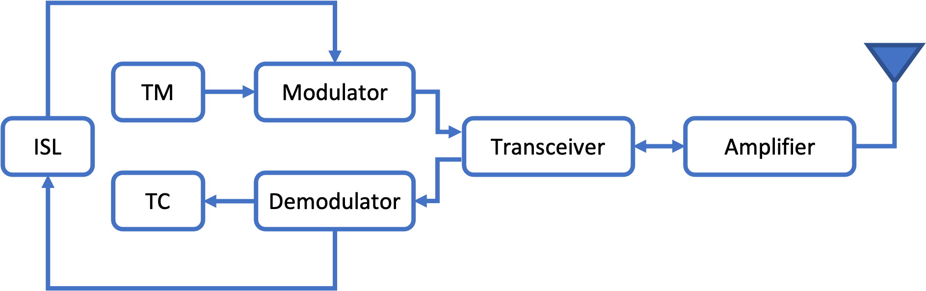
Figure 9: ISL communications: The block diagram illustrates the inter-satellite link communication system, including the S-band patch antenna, the amplifier, the modulator and demodulator blocks, and the Telemetery (TM) and Telecommand (TC) blocks, which are discussed in Section 8

.

Table 8: Communication and operational requirements

Ground station passes	1 pass every 2 days; 1 hour window
Antenna size	98 $\times$ 98 mm
Data volume per pass per satellite	40–400 MB
Uplink and downlink frequency	2.45 GHz
Power available for communication	4 W (average)
Downlink data rate	$\geq$ 20 mbit/sec

8 Communication

Communication is a crucial aspect of the APIS mission for autonomy, satellite navigation, and science payload processing. A summary of all the communication and operational requirements is listed in Table 8. We discuss the Inter-satellite and Earth-based communication in this section.

8.1 Inter-satellite link (ISL)

Individual satellites need inter-satellite links (ISLs) to share information with each other and to transmit the information collected by scientific exploration to the ground center. Thus, the satellites also utilize satellite-to-ground communication. A simple block diagram in Figure 9 shows the communication system loop for the ISL in the satellite swarm. For the scientific goals of the APIS mission, every satellite must establish a high data rate radio connection with the other satellites, and include a transceiver. The antenna must have sufficient gain and transmission power, and the transceiver must meet the data requirements. According to the existing patch antennas and transceivers available on the market, we investigated five possible antenna systems for the APIS satellites, which are listed in Table 6. Considering the size of the satellite and the data transmission requirements, the S-band patch antenna produced by Endurosat is the chosen antenna for the APIS mission. Along similar lines, we considered four types of transceivers for the APIS mission as shown in Table 7. The transceiver made by ECM Space Technologies GmbH company is attractive in terms of power, volume and mass, which is, therefore, the chosen transceiver for the APIS mission. The ECM transceiver will employ QPSK for transmission and BPSK reception, and offers a data transmission rate of up to $20$ Mbps. A summary of ISL budget for a satellite pair is presented in Table 9.

8.2 Uplink and Downlink to Earth

APIS mission satellites are small in size and restricted in power supply, so at higher orbits the satellites will not be able to communicate directly with the ground-based antennas in full bandwidth. At these orbits, Mobile Ad-Hoc Network (MANET) technology can be used to send information to ground stations. The swarm uses ISLs to hop data from satellite to satellite until the satellite closest to the Earth can send the data to the ground [70]. During Earth fly-by at the perigee, the satellites employ multi-hop communication for data downlink, as illustrated in Figure 7(b). The MANET system is highly dynamic, fault-resistant, and autonomous, which is advantageous for APIS satellites to communicate data to ground stations. To reduce design complexity, the communications from satellite-to-Earth and ISLs will be combined. Delay Tolerant Networking (DTN) technology will store and transmit data back to ground stations, following processing, once satellite have reached a low-altitude location, providing reliable communication in case of network connection interruption [71].

Using the THEMIS mission as a reference, we estimate a data rate of up to $500$ bytes/second from all of the science payloads [31]. The APIS satellites can have up to 20 Mbit/s of data downlink. To manage thermal issues and data packet loss we assume a guaranteed data rate of 1 Mbit/s. With one hour of contact to the ground station, each satellite can transmit up to 400 MB. Assuming a 50% success rate of package transmission, as commonly used [31], the data transmission per perigee pass reduces to 200 MB. Furthermore, assuming half the data consists of telemetry and housekeeping data, we can then assume a successfull transmission of up to 100 MB of science data per perigee pass. Refer to Table 9 for a detailed link budget.

Table 9: Communication Link Budgets of the satellites in the APIS mission

(a) Inter-Satellite Link			(b) Uplink			(c) Downlink
ISL Frequency:	2150 MHz		Uplink Frequency:	2150 MHz		Downlink Frequency:	2150 MHz
Distance:	35040.5 km		Distance:	35040.5 km		Distance:	18846.8 km
1st Spacecraft:			Ground Station:			Spacecraft:
Spacecraft Transmitter Power Output:	8.0 W		Transmitter Power Output:	50.0 W		Spacecraft Transmitter Power Output:	8.0 W
	9.0 dBW			17.0 dBW			9.0 dBW
	39.0 dBm			47.0 dBm			39.0 dBm
Spacecraft Transmission Line Losses:	-1.0 dB		Transmission Line Losses:	-3.0 dB		Spacecraft Transmission Line Losses:	-1.0 dB
S/C Connector, Filter or In-Line Switch Losses:	0.0 dB		S/C Connector, Filter or In-Line Switch Losses:	-1.0 dB		S/C Connector, Filter or In-Line Switch Losses:	0.0 dB
Spacecraft Antenna Gain:	8.3 dBiC		Antenna Gain:	31.4 dBiC		Spacecraft Antenna Gain:	8.3 dBiC
Spacecraft EIRP:	46.3 dBm		Ground Station EIRP:	74.3 dBW		Spacecraft EIRP:	46.3 dBm
Crosslink Path:			Uplink Path:			Downlink Path:
Spacecraft Antenna Pointing Loss:	-1.0 dB		Ground Station Antenna Pointing Loss:	-1.0 dB		Spacecraft Antenna Pointing Loss:	-1.0 dB
Antenna Polarization Loss:	-1.5 dB		Antenna Polarization Loss:	-4.0 dB		Antenna Polarization Loss:	-1.5 dB
Path Loss:	-190.0 dB		Path Loss:	-190.0 dB		Path Loss:	-184.6 dB
Atmospheric Loss:	0 dB		Atmospheric Losses:	-3 dB		Atmospheric Loss:	-2.2 dB
Isotropic Signal Level at Spacecraft:	-146.4 dBm		Isotropic Signal Level at Ground Station:	-124.7 dBm		Isotropic Signal Level at Ground Station:	-143.2 dBm
2nd Spacecraft:			Spacecraft:			Ground Station:
2nd Spacecraft Antenna Pointing Loss:	0.0 dB		Spacecraft Antenna Pointing Loss:	0.0 dB		Ground Station Antenna Pointing Loss:	-2.0 dB
2nd Spacecraft Antenna Gain:	8.3 dBiC		Spacecraft Antenna Gain:	8.3 dBiC		Ground Station Antenna Gain:	31.35 dBic
2nd Spacecraft Transmission Line Losses:	-1 dB		Spacecraft Transmission Line Losses:	-1 dB		Ground Station Transmission Line Losses:	-1 dB
S/C Transmission Line Coefficient:	0.7943		S/C Transmission Line Coefficient:	0.7943		G.S. Transmission Line Coefficient:	0.7943
2nd Spacecraft Effective Noise Temperature:	250 K		Spacecraft Effective Noise Temperature:	250 K		Ground Station Effective Noise Temperature:	542 K
2nd Spacecraft Figure of Merit (G/T):	-16.7 dB/K		Spacecraft Figure of Merit (G/T):	-16.7 dB/K		Ground Station Figure of Merit (G/T):	3.0 dB/K
S/C Signal-to-Noise Power Density (S/No):	65.5 dBHz		S/C Signal-to-Noise Power Density (S/No):	87.3 dBHz		G.S. Signal-to-Noise Power Density (S/No):	86.4 dBHz
System Desired Data Rate:	$1.00\times 10^{7}$ bps		System Desired Data Rate:	$2.00\times 10^{7}$ bps		System Desired Data Rate:	$2.00\times 10^{7}$ bps
	50.0 dBHz			73.0 dBHz			73.0 dBHz
System Required Eb/No:	10 dB		Telemetry System Required Eb/No:	10 dB		Telemetry System Required Eb/No:	10 dB
System Link Margin:	5.5 dB		System Link Margin:	4.2 dB		System Link Margin:	3.4 dB

9 On-board processing

The On-Board Computer (OBC) is a crucial component to the functionality of the mission and is responsible for reading, collecting, and processing sensor information from the ADCS, GNSS, and communications systems, which includes executing Telemetry, Tracking and Command (TTC) operations, and storing on-board health data. Additionally, the OBC is responsible for maintaining the On-Board Timers (OBT) for synchronization, localization, control, and performing inertial referencing calculations [72]. In addition, the OBC must execute all expected tasks while abiding to bus requirements. Thus, we need to keep the power consumption and mass low, with the frequency and Total Ionizing Dose (TID) high. Higher frequency ensures tasks can be completed within the lowest necessary time, however, this requires high power consumption. Thus, both frequency and power must be balanced.

Since the APIS mission is to study the magnetosphere outside of LEO, radiation hardening of the OBC processor is an important requirement, as the charged particles ejected from the Sun can cause detrimental and undesired effects to the on-board electronics [73, 74]. Based on the NASA RHESE project, radiation hardening of OBC components is recommended through: material hardening of OBC components and shielding; the inclusion of redundant hardware; software verification and reconfigurability [73]. The measure of accumulated radiation a device can withstand prior to becoming unreliable is known as the TID, which acts as a metric for the life expectancy of the device [74], and sets the parameters for radiation hardening. A higher TID ensures a higher life expectancy for the electronics.

A trade study was completed to compare the available options viable for the APIS mission listed in Table 10. All three options have similar dimensions, though, ISISpace offers the highest operating frequency at the cost of higher power consumption. However, for the APIS mission, mass is a critical criteria, and hence we chose the IMT component, weighing nearly half the mass of the remaining two options.

The satellite swarm in the APIS mission will comprise of autonomous satellites, and to that end will each achieve (a) Self-configuration, (b) Self-optimization, (c) Self-healing and (d) Self-protection, during mission operation [75]. If an autonomous system has the authority to make changes to its command, and behaves in an unexpected way, it will reduce the level of trust between the system and its operators [76]. Changes in trust levels will complicate mission design and may necessitate the creation and installation of safeguards that further increase system complexity. In addition to exploiting autonomy, the APIS mission will facilitate distributed functionality, enabling emergent behavior of the satellite swarm.

To enable the emergent behavior of the swarm satellites, we need to partner an appropriate operating system with the OBC. NASA conducted research on the feasibility of using COTS technology for the Command and Data Handling (CDH) system of a swarm of satellites [77]. The study used an android operating system with specific programming to relay data from both satellite-to-satellite and satellite-to-ground stations, demonstrating the feasibility of the satellite swarm behavior using COTS software. We recommend using an adapted version of FreeRTOS, which can process, allocate, and communicate tasks in a large-scale multi-processor network with reduced network congestion and communication energy [78].

Table 10: Potential OBC options and specifications

OBC Option	Power Consumption (mW)	Mass (g)	Dimensions $\mathbf{l\times w\times h}$ (mm)	Frequency (MHz)	Total  Ionizing Dose (kRad)
ISIS	400	76	$96\times 90\times 12.4$	400	N/A
CubeComputer	200	50-70	$90\times 96\times 10$	48	20
IMT	300	38	$96\times 90\times 10$	200	15

Table 11: Power budget

System	Average (W)	Idle (W)	Peak (W)
Payload	10	1	250
DHS	2	2	2
IMU	2.4	2.4	2.4
RF/ISL Link	13	1.7	38
ADCS/OBC	10	10	10
Reaction Wheels	2.4	2.4	4
Magnetic Torquers	0.175	0.175	1.2
Thermal	8	5	15
Power Electronics	4	4	4
Battery Charge	10	5	20
2% Losses	1.2395	0.6735	7.892
Total Load:	63.2	34.3	354.4

10 Power system

The various sub-systems in the APIS satellite, e.g., navigation, communication and OBC are fueled by the on-board power system. The electrical power system deals with the generation, storage, monitoring, control, and distribution of electrical power. A summary of the power budget requirements for various APIS satellite sub-systems and all the scientific payloads discussed in the previous sections, are listed in Table 11. The total average power demand for an APIS satellite is estimated at 63.2 watts. We briefly introduce various sub-systems within the power system.

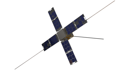
(a)

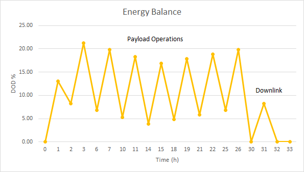
(b)

Figure 10: (a) APIS satellite solar panels: An illustration of the solar panels deployed in an APIS satellite. The solar panels are fixed in a windmill fashion to ensure the panels are consistently facing the Sun during orbit, gaining maximal solar energy for powering satellite system. (b) APIS satellite energy balance: The typical energy balance for an APIS satellite battery over the course of one orbit is presented.

• Generation: Solar panels are the safest, and cheapest choice for the missions for near-Earth orbit. The state of the art AM0 ATJ (Advanced Triple Junction) or ZQJ (Azur Quad Junction) solar cells available give greater than $35$% beginning of life efficiency, and will produce $245$ W/m² [79]. The battery acts as a backup support whenever the solar cells or array unable to point towards the Sun during maneuvers or payload operations. The solar panel is deployable and fixed, instead of variable, for Sun-tracking. Moreover, body-mounted solar cells cannot meet the power requirements of the satellite swarm, thus, deployable solar panels are necessary. There are two panels for each side in a fixed configuration, and the solar panel parameters are presented in Table 13. We have fixed a windmill design of the solar panels such that they are always pointing towards the Sun during their orbit, which is illustrated in Figure 10(a).

• Storage: Lithium Ion (Li-Ion) cells are reliable in both small and large satellite applications, and their performance can be further enhanced with carbon nanotube electrodes [80]. Figure 10 shows the energy balance for the battery, where the estimated charge and discharge cycles are illustrated during mission life. For a five-year mission, a safe limit with a margin for Depth of Discharge (DoD) of $20$% is about $30000$ cycles. With these constraints, we choose the LG18650MJ1 Li-Ion cell with the battery sizing as listed in Table 13.

• Power control and monitoring: Traditionally, the power control unit regulates power from the solar panels and batteries, consisting of three units to adjust the output and charge the battery pack. A more optimal system includes a digitally integrated array control and battery charging unit [81]. Additionally, the system determines the health of critical power elements and has a set of protection against overloads, undervoltage, and overvoltage occurrences.

• Power distribution: Power distribution systems can be distributed or centralized. The best choice for the APIS satellites are Solid-State Power Controllers (SSPC), as they are more reliable than electromechanical relays and are re-triggerable in case of faults caused by noise, electromagnetic interference or radiation effects [82]. For satellites of 12U size, a centralized, regulated distribution will be efficient in mass and volume with all bus systems powered with a single Direct Current/Direct Current (DC/DC) module. We choose dedicated DC/DC converters for redundant systems to avoid single-point failures, where one failure could otherwise affect the entire satellite. The payload is sensitive, requiring completely different voltage scales, and should include local DC/DC converters, a low drop-out regulator, and a switch to disconnect the system from the source for isolating a fault if required.

Table 12: Solar panel parameters

Parameter	Value
Face area	0.04 m2
Generation @ BOL	78.5 W
ATJ/ZQJ 0.5 mA cells in parallel	4
Number of strings	4
Regulation control	IAC-BC
Total Panel Area (2 panels $\times$ 4 panels)	0.32 m2
Generation @ EOL	67 W
Number of cells in series	14
Power loss per string	16 W
Estimated weight	1.4 kg

Table 13: Battery parameters

Parameter	Value
Allowed DoD	<20%
Load power	Peak: $\sim$54 W Idle: 34 W
Discharge at average voltage	Peak: 10 A (100 ms/3 s) Nominal: 1.1 A
Regulation control	IAC-BC
Final battery size	8S4P
Number of cells in series	8
Total cycles	$\sim$30 000
Cell	LG18650MJ1 3.5 Ah
Capacity	400 Wh

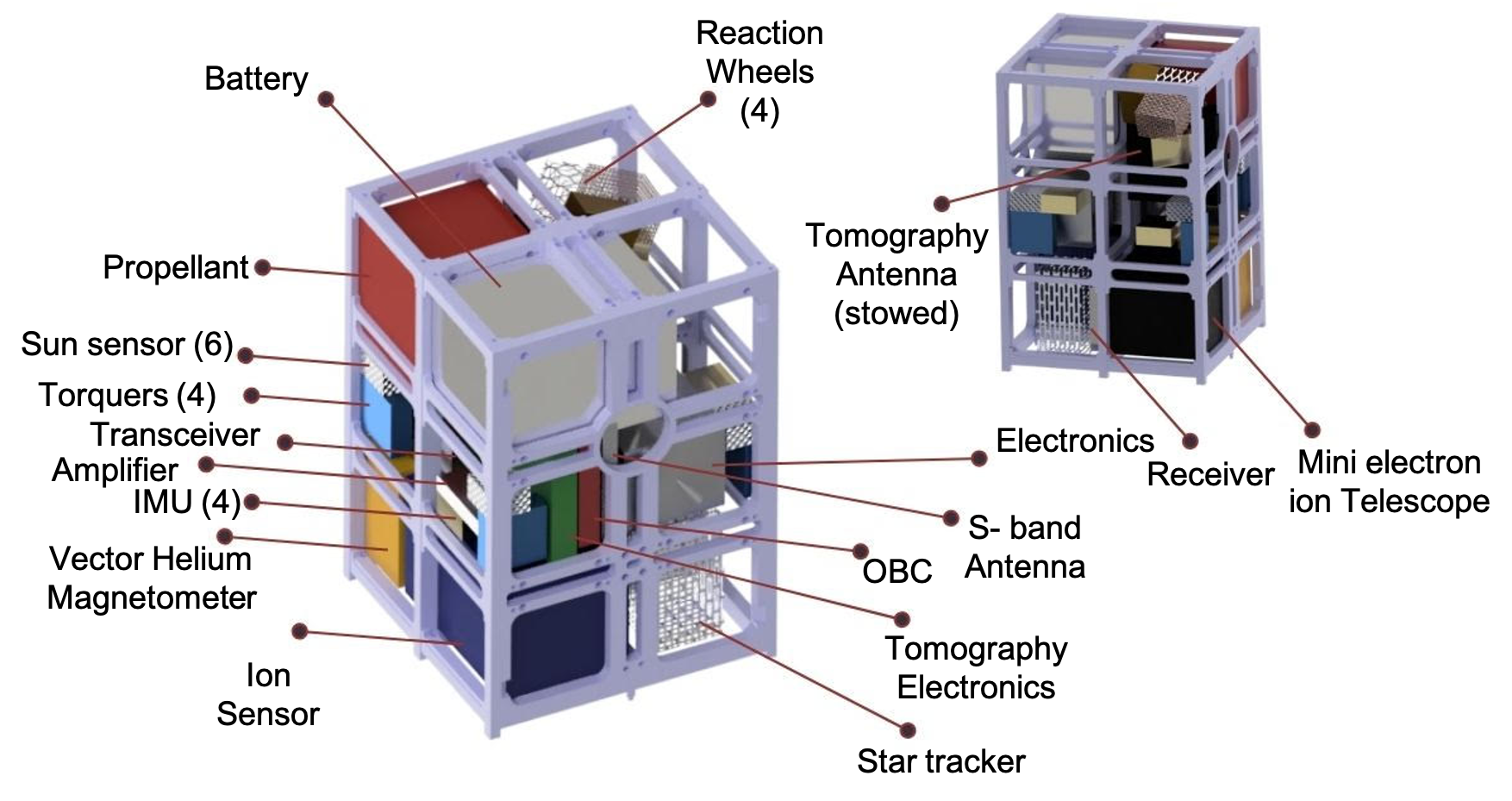
Figure 11: APIS satellite decomposition: A simplified view of the APIS 12U satellite along with the subsystems and scientific payloads. A list of all chosen COTS components are listed in Table 14.

Table 14: Mass budget

System	Component	Mass	Dimension	Volume
		(kg)	(mm)	(mm3)
Payload	Ion Sensor	1.37	100 x 100 x 150	500000
	Vector Helium Magnetometer	0.82	100 x 100 x 50	500000
	Mini Electron ion Telescope	1.1	100 x 100 x 90	900000
	Tomography Electronics	1	100 x 100 x 20	200000
	Tomography Antenna	1	15000 x 27 (deployed)	-
	Tomography Antenna		90 x 90 x 40 (stowed)	324000
	Magnetic Boom	0.4	8 x 680	5440
OBC	-	0.5	96 x 90 x 17	146880
ADCS	Reaction Wheels (4 nos)	0.52	42 x 42 x 19	33516
	Torquers (4 no.)	0.8	96 x 90 x 17	146880
	Star Tracker (1 no.)	0.36	100 x 55 x 50	275000
	Sun Sensor (6 nos)	0.21	34 x 40 x 20	27200
	IMU (4 no.)	0.22	39 x 45 x 22	38610
GNSS	Receiver	0.1	71 x 46 x 11	35926
	Antenna	0.1	-	-
Frame structure	-	1.5	226 x 226 x 340	-
Communications	S-Band Antenna	0.07	98 x 98 x 12	115248
	Amplifier	0.3	68 x 45 x 12	36720
	Transceiver	0.1	95 x 50 x 55	261250
Power system	Solar Panel	1.4	200 x	40000
			200 (8 nos)	-
	Battery	1.8	96 x 96 x 144	1327104
	Electronics	0.5	80 x 80 x 70	448000
Thermal Control	-	1.5	N/A	-
Propulsion System	Propellant	1.2	96 x 96 x 96	884736
	Dry Mass	4	-	-
Misc/Harness	-	1	-	-
	Total	21.87		6246510

11 Conclusion

The APIS mission aims to characterize plasma processes and measure the effect of the solar wind on Earth’s magnetosphere. We propose a swarm of 40 CubeSats in two highly-elliptical orbits around the Earth, to investigate both the magnetotail and the Sun-ward magnetosphere, with a focus on radio tomography in the magnetotail. The APIS satellites will employ radio tomography, and carry various in-situ measurement systems on-board, e.g., super-thermal ion spectrograph, miniaturized electron and ion telescope, and vector helium magnetometer to provide large-scale maps of plasma density and turbulence in the magnetotail. We estimate the minimum science requirement, of radio tomography in the magnetotail to be achieved in the course of the first 3–4 months into the mission. At the end of the first year, all the key science phases will be completed.

Towards the satellite design, various subsystems have been studied, e.g., navigation, communication, on-board processing, power and propulsion systems. A preliminary investigation on the mass and volume budget of a single satellite was conducted, and a summary of all payloads and components are listed in Table 14. We show that COTS technologies available today can be used to meet the outlined science requirements. Table 14 indicates that the APIS mission can be designed using homogeneous CubeSats, with a possible 12U form factor (226 mm $\times$ 226 mm $\times$ 340 mm). A satellite decomposition is shown in Figure 11, which encompasses all the subsystems discussed in the previous sections and the scientific payloads. We favor the skin-frame structure over a simple frame structure because of its resistance to bending, tensional and axial forces [83], and an aluminum and carbon-fiber-epoxy as the material for our bus. The APIS project is a partially funded by NASA, though this is beyond the scope of this work.

12 Future work

A comprehensive system design is an on-going investigation, and will be presented in subsequent work. As stated earlier, the power and mass budgets are preliminary and need a through review. Furthermore, we would like to investigate various thermal control methods (including both active and passive systems), suitable for the APIS mission. In addition to a detailed system model, some of the key future challenges involve distributed algorithms for swarm behaviour, including energy-efficient communication [84], smart autonomous navigation [85], distributed processing [86], attitude control [87], and in-depth mission planning [88, 89]. Furthermore, significant advances in propulsion technology [90], and miniaturization of satellite subsystems and payloads in the upcoming decades will yield smaller satellites and larger swarms, subsequently benefiting the APIS mission [65].

Figure 12: APIS mission patch: APIS is adopted from the genus name Apis, meaning ‘Bee’ in Latin, which was an inspiration for the APIS mission patch designed during this study

13 Acknowledgement

The APIS mission design study was part of the International Space University Space Studies Program in 2019 (ISU-SSP19) as the Next Generation Space Systems: Swarms Team Project, which is partially funded by NASA. This 9-week intense project was conducted by a team of 32 members from 16 nationalities, who are drawn from diverse professional backgrounds within the space sector, which include but are not limited to engineers, scientists, lawyers and managers. The authors of this publication include the APIS team, the Chairs Dr. Jacob Cohen, Anh Nguyen and Andrew Simon-Butler, and the support staff Ruth McAvinia. The name of the project is adopted from the genus name Apis, meaning ‘Bee’ in Latin, which was an inspiration for the APIS mission patch designed during this study (see Figure 12).

The authors would like to thank the Editor, the anonymous reviewers, and Dr. Prem Sundaramoorthy for their constructive comments, which helped improve the quality this article.

References

-
[1]
C. J. Schrijver, G. L. Siscoe,
Heliophysics:
Plasma Physics of the Local Cosmos, Cambridge University Press, Cambridge,
2009.
doi:10.1017/CBO9781107340657.
URL http://ebooks.cambridge.org/ref/id/CBO9781107340657 -
[2]
M. Kivelson, M. Kivelson, C. Russell,
Introduction to Space
Physics, Cambridge atmospheric and space science series, Cambridge
University Press, 1995.
URL https://books.google.nl/books?id=qWHSqXGfsfQC - [3] B. A. Smith, L. A. Soderblom, T. V. Johnson, A. P. Ingersoll, S. A. Collins, E. M. Shoemaker, G. E. Hunt, H. Masursky, M. H. Carr, M. E. Davies, A. F. Cook, J. Boyce, G. E. Danielson, T. Owen, C. Sagan, R. F. Beebe, J. Veverka, R. G. Strom, J. F. McCauley, D. Morrison, G. A. Briggs, V. E. Suomi, The Jupiter system through the eyes of Voyager 1, Science 204 (4396) (1979) 951–972. doi:10.1126/science.204.4396.951.
- [4] J. T. Clarke, J. Nichols, J. C. Gérard, D. Grodent, K. C. Hansen, W. Kurth, G. R. Gladstone, J. Duval, S. Wannawichian, E. Bunce, S. W. Cowley, F. Crary, M. Dougherty, L. Lamy, D. Mitchell, W. Pryor, K. Retherford, T. Stallard, B. Zieger, P. Zarka, B. Cecconi, Response of Jupiter’s and Saturn’s auroral activity to the solar wind, Journal of Geophysical Research: Space Physics 114 (5) (2009) 1–20. doi:10.1029/2008JA013694.
- [5] R. M. Winslow, B. J. Anderson, C. L. Johnson, J. A. Slavin, H. Korth, M. E. Purucker, D. N. Baker, S. C. Solomon, Mercury’s magnetopause and bow shock from MESSENGER Magnetometer observations, Journal of Geophysical Research: Space Physics 118 (5) (2013) 2213–2227. doi:10.1002/jgra.50237.
-
[6]
J. N. Pelton, F. Allahdadi (Eds.),
Handbook of Cosmic
Hazards and Planetary Defense, Springer International Publishing, Cham,
2015.
doi:10.1007/978-3-319-03952-7.
URL http://link.springer.com/10.1007/978-3-319-03952-7 -
[7]
D. J. Barnhart, T. Vladimirova, M. N. Sweeting,
Very-small-satellite
design for distributed space missions, Journal of Spacecraft and Rockets
44 (6) (2007) 1294–1306.
URL https://arc.aiaa.org/doi/pdfplus/10.2514/1.28678 - [8] J. R. Behrens, B. Lal, Exploring trends in the global small satellite ecosystem, New Space 7 (3) (2019) 126–136.
-
[9]
E. Buchen,
Small
satellite market observations, in: Proceedings of the Small Satellite
Conference, 2015.
URL https://digitalcommons.usu.edu/cgi/viewcontent.cgi?article=3215&context=smallsat - [10] R. Sandau, Status and trends of small satellite missions for earth observation, Acta Astronautica 66 (1-2) (2010) 1–12.
- [11] V. S. Reddy, The spacex effect, New Space 6 (2) (2018) 125–134.
- [12] V. Angelopoulos, The THEMIS mission, Space Science Reviews 141 (1-4) (2008) 5–34. doi:10.1007/s11214-008-9336-1.
- [13] C. Escoubet, M. Fehringer, M. Goldstein, The cluster mission, Annales Geophysicae 19 (2001) 1197–1200. doi:10.5194/angeo-19-1197-2001.
- [14] T. Karlsson, F. Plaschke, H. Hietala, M. Archer, X. Blanco-Cano, P. Kajdič, P. A. Lindqvist, G. Marklund, D. J. Gershman, Investigating the anatomy of magnetosheath jets - MMS observations, Annales Geophysicae 36 (2) (2018) 655–677. doi:10.5194/angeo-36-655-2018.
- [15] R. M. Young, Updated heliostorm warning mission: Enhancements based on new technology, Collection of Technical Papers - AIAA/ASME/ASCE/AHS/ASC Structures, Structural Dynamics and Materials Conference 7 (2007) 6662–6674.
- [16] J. Green, D. Draper, H. Grant, J. Rall, Scientific discovery and geomagnetic monitoring in earth orbit using small satellite systems, Handbook of Small Satellites: Technology, Design, Manufacture, Applications, Economics and Regulation (2020) 639–657.
- [17] L. Plice, A. D. Perez, S. West, Helioswarm: Swarm mission design in high altitude orbit for heliophysics, in: AAS/AIAA Astrodynamics Specialist Conference, Portland, ME, USA, 2019.
- [18] R. M. Millan, R. von Steiger, M. Ariel, S. Bartalev, M. Borgeaud, S. Campagnola, J. C. Castillo-Rogez, R. Fléron, V. Gass, A. Gregorio, et al., Small satellites for space science: A cospar scientific roadmap, Advances in space research 64 (8) (2019) 1466–1517.
- [19] L. Blum, L. Kepko, D. Turner, C. Gabrielse, A. Jaynes, S. Kanekal, Q. Schiller, J. Espley, D. Sheppard, L. Santos, et al., The gtosat cubesat: scientific objectives and instrumentation, in: Micro-and Nanotechnology Sensors, Systems, and Applications XII, Vol. 11389, International Society for Optics and Photonics, 2020, p. 113892E.
- [20] R. L. Bishop, R. Walterscheid, J. Clemmons, A. Barjatya, L. O. Gunter, The low-latitude ionosphere/thermosphere enhancements in density (llited) mission, in: Proceedings of the Small Satellite Conference, 2019.
- [21] J. Klenzing, R. Davidson, S. Jones, C. Martinis, K. Zawdie, G. Earle, J. Smith, A. Halford, S. Noel, N. Paschalidis, et al., The petitsat mission–science goals and instrumentation, Advances in Space Research 66 (1) (2020) 107–115.
- [22] C. E. DeForest, S. E. Gibson, M. Beasley, R. C. Colaninno, R. Killough, W. Kosmann, G. T. Laurent, D. R. McMullin, Polarimeter to unify the corona and heliosphere (punch): Imaging the corona and solar wind as a single system, in: AGU Fall Meeting Abstracts, Vol. 2019, 2019, pp. SH43B–06.
- [23] J. Westerhoff, G. Earle, R. Bishop, G. R. Swenson, S. Vadas, J. Clemmons, R. Davidson, L. Fanelli, C. Fish, V. Garg, et al., Laice cubesat mission for gravity wave studies, Advances in Space Research 56 (7) (2015) 1413–1427.
- [24] J. H. Hecht, L. J. Gelinas, D. A. Hinkley, J.-H. Yee, A. B. Christensen, S. C. Solomon, G. Crowley, The daili (daily atmosphere and ionosphere limb imager) cubesat mission, in: AGU Fall Meeting Abstracts, Vol. 2019, 2019, pp. SA44A–08.
- [25] M. I. Desai, F. Allegrini, R. W. Ebert, K. Ogasawara, M. E. Epperly, D. E. George, E. R. Christian, S. G. Kanekal, N. Murphy, B. Randol, The CubeSat Mission to Study Solar Particles, IEEE Aerospace and Electronic Systems Magazine 34 (4) (2019) 16–28. doi:10.1109/maes.2019.2917802.
-
[26]
K. G. Klein, O. Alexandrova, J. Bookbinder, D. Caprioli, A. W. Case, B. D. G.
Chandran, L. J. Chen, T. Horbury, L. Jian, J. C. Kasper, O. L. Contel, B. A.
Maruca, W. Matthaeus, A. Retino, O. Roberts, A. Schekochihin, R. Skoug,
C. Smith, J. Steinberg, H. Spence, B. Vasquez, J. M. TenBarge, D. Verscharen,
P. Whittlesey, Multipoint
Measurements of the Solar Wind: A Proposed Advance for Studying Magnetized
Turbulence (2019).
arXiv:1903.05740.
URL http://arxiv.org/abs/1903.05740 -
[27]
L. Guan, L. Kepko,
Magnetospheric
Constellation: Tracing the flow of mass and energy from the solar wind
through the magnetosphere 1–8.
URL http://www8.nationalacademies.org/SSBSurvey/DetailFileDisplay.aspx?id=746& -
[28]
National Research Council, Solar and
Space Physics: A Science for a Technological Society, National Academies
Press, Washington, D.C., 2013.
doi:10.17226/13060.
URL http://www.nap.edu/catalog/13060 -
[29]
National Academy of Sciences,
Achieving Science with CubeSats:
Thinking Inside the Box, National Academies Press, Washington, D.C., 2016.
doi:10.17226/23503.
URL https://www.nap.edu/catalog/23503 - [30] Y. Zhai, S. A. Cummer, J. L. Green, B. W. Reinisch, M. L. Kaiser, M. J. Reiner, K. Goetz, Magnetospheric radio tomographic imaging with IMAGE and Wind, Journal of Geophysical Research: Space Physics 116 (12) (2011) 1–8. doi:10.1029/2011JA016743.
- [31] V. Angelopoulos, The THEMIS mission, Space Science Reviews 141 (1-4) (2008) 5–34. doi:10.1007/s11214-008-9336-1.
- [32] W. Matthaeus, The essential role of multi-point measurements in turbulence investigations: the solar wind beyond single scale and beyond the Taylor Hypothesis, Tech. Rep. February 2019 (2019).
-
[33]
NASA Science and Technology Definition Team for the Magnetospheric
Constellation Mission, The
Magnetospheric Constellation (MC), Tech. rep., NASA (2004).
URL http://stp.gsfc.nasa.gov/missions/ - [34] R. E. Ergun, D. E. Larson, T. Phan, D. Taylor, S. Bale, C. W. Carlson, I. Roth, V. Angelopoulos, J. Raeder, T. Bell, U. S. Inan, J.-L. Bougeret, R. Manning, Feasibility of a multisatellite investigation of the Earth’s magnetosphere with radio tomography, Journal of Geophysical Research: Space Physics 105 (A1) (2000) 361–373. doi:10.1029/1999ja900170.
- [35] J. Etcheto, Y. De Javel, M. Petit, The ISEE Electron Density Experiment, IEEE Transactions on Geoscience Electronics 16 (3) (1978) 231–238. doi:10.1109/TGE.1978.294553.
- [36] R. Leitinger, Data from orbiting navigation satellites for tomographic reconstruction, International Journal of Imaging Systems and Technology 5 (2) (1994) 86–96. doi:10.1002/ima.1850050205.
- [37] K. Davies, Ionospheric radio, no. 31 in {IEE} electromagnetic waves series, London, 1989.
- [38] SpaceX, Falcon 9, https://www.spacex.com/vehicles/falcon-9/, accessed 2020-09-28.
-
[39]
J. Goodwin, P. Wegner,
Evolved expendable
launch vehicle secondary payload adapter - Helping technology get to space.
arXiv:https://arc.aiaa.org/doi/pdf/10.2514/6.2001-4701, doi:10.2514/6.2001-4701.
URL https://arc.aiaa.org/doi/abs/10.2514/6.2001-4701 - [40] P. M. Wegner, J. Ganley, J. R. Maly, EELV secondary payload adapter (ESPA): providing increased access to space, in: 2001 IEEE Aerospace Conference Proceedings (Cat. No. 01TH8542), Vol. 5, IEEE, 2001, pp. 2563–2568.
- [41] J. Maly, G. Sanford, A. Williams, L. Berenberg, ESPA class redefined, in: Proceedings of the AIAA/USU Conference on Small Satellites, 2017, pp. SSC17–IV.
-
[42]
Y. Miyazaki, Deployable
Techniques for Small Satellites, Proceedings of the IEEE 106 (3) (2018)
471–483.
doi:10.1109/JPROC.2018.2799608.
URL http://ieeexplore.ieee.org/document/8293792/ - [43] F. Barao, AMS—alpha magnetic spectrometer on the international space station, Nuclear Instruments and Methods in Physics Research Section A: Accelerators, Spectrometers, Detectors and Associated Equipment 535 (1-2) (2004) 134–138.
- [44] R. T. Rajan, R.-v. Schaijk, A. Das, J. Romme, F. Pasveer, Reference-Free Calibration in Sensor Networks, IEEE Sensors Letters 2 (3) (2018) 1–4. doi:10.1109/lsens.2018.2866627.
-
[45]
L. Balzano, R. Nowak,
Blind
calibration of sensor networks, Proceedings of the 6th international
conference on Information processing in sensor networks - IPSN ’07 (2007)
79doi:10.1145/1236360.1236372.
URL http://portal.acm.org/citation.cfm?doid=1236360.1236372 - [46] Y. Wang, S. Member, A. Yang, X. Chen, P. Wang, Y. Wang, S. Member, H. Yang, S. Member, A Deep Learning Approach for Blind Drift Calibration of Sensor Networks, IEEE Sensors Journal 13 (2017) 1558–1748. doi:10.1109/JSEN.2017.2703885.
-
[47]
B. Sundararaman, U. Buy, A. D. Kshemkalyani,
Clock
synchronization for wireless sensor networks: a survey, Ad Hoc Networks
3 (3) (2005) 281–323.
doi:10.1016/j.adhoc.2005.01.002.
URL https://linkinghub.elsevier.com/retrieve/pii/S1570870505000144 -
[48]
R. T. Rajan, M. Bentum, A.-J. Boonstra,
Synchronization for
space based ultra low frequency interferometry, in: 2013 IEEE Aerospace
Conference, IEEE, 2013, pp. 1–8.
doi:10.1109/AERO.2013.6496931.
URL http://ieeexplore.ieee.org/document/6496931/ - [49] D. W. Allan, Statistics of Atomic Frequency Standards, Proceedings of the IEEE 54 (2) (1966) 221–230. doi:10.1109/PROC.1966.4634.
-
[50]
Silicon Labs,
Si570/Si571
10Mhz to 1.4Ghz I2C Programmable XO/VCXO Features Applications Description
(2018) 1–36.
URL https://www.silabs.com/documents/public/data-sheets/si570.pdf -
[51]
R. T. Rajan, A.-J. van der Veen,
Joint Ranging and
Synchronization for an Anchorless Network of Mobile Nodes, IEEE
Transactions on Signal Processing 63 (8) (2015) 1925–1940.
doi:10.1109/TSP.2015.2391076.
URL http://ieeexplore.ieee.org/document/7006748/ - [52] M. Kaufmann, A. Tuysuz, J. W. Kolar, C. Zwyssig, High-speed magnetically levitated reaction wheels for small satellites, 2016 International Symposium on Power Electronics, Electrical Drives, Automation and Motion (Speedam) (2016) 28–33. doi:10.1109/SPEEDAM.2016.7525889.
- [53] S. S. Nudehi, U. Farooq, A. Alasty, J. Issa, Satellite attitude control using three reaction wheels, Proceedings of the American Control Conference (2008) 4850–4855doi:10.1109/ACC.2008.4587262.
- [54] Blue Canyon Tech., RWP015 (MicroWheel), https://storage.googleapis.com/blue-canyon-tech-news/1/2020/06/BCT_DataSheet_Components_ReactionWheels_06_2020.pdf, accessed 2020-09-28.
- [55] T. Inamori, S. Nakasuk, Application of Magnetic Sensors to Nano and Micro-Satellite Attitude Control Systems, 2012. doi:10.5772/34307.
- [56] ISISpace, Magnetorquer Board (iMTQ), https://www.isispace.nl/product/isis-magnetorquer-board/, accessed 2020-09-28.
- [57] Blue Canyon Tech., Standard NST, https://storage.googleapis.com/blue-canyon-tech-news/1/2020/06/BCT_DataSheet_Components_StarTrackers_06_2020.pdf, accessed 2020-09-28.
- [58] NewSpace Systems (NSS), NFSS-411 Sun sensor, https://www.cubesatshop.com/product/digital-fine-sun-sensor/, accessed 2020-09-28.
- [59] Sensonor, STIM377H Inertial Measurement Unit, https://www.sensonor.com/products/inertial-measurement-units/stim377h/, accessed 2020-09-28.
- [60] J. Huff, A. Schultz, M. U. de Haag, Assured relative and absolute navigation of a swarm of small uas, in: 2017 IEEE/AIAA 36th Digital Avionics Systems Conference (DASC), 2017, pp. 1–10.
- [61] NovAtel, OEM719 Multi-Frequency GNSS Receiver, https://www.gnssystems.se/kopia-pa-span-igm-s1-gnss-ins-recei, accessed 2020-09-28.
-
[62]
I. Borg, P. J. F. Groenen, P. Mair,
Applied
Multidimensional Scaling, 2013.
doi:10.1007/978-3-642-31848-1.
URL http://link.springer.com/10.1007/978-3-642-31848-1 -
[63]
B.-H. Lee, K.-H. Oh, T. Hatanaka, H.-S. Ahn,
Distributed estimation
of both position and orientation for networked systems on the sphere, in:
2018 Annual IEEE International Systems Conference (SysCon), IEEE, 2018, pp.
1–6.
doi:10.1109/SYSCON.2018.8369505.
URL https://ieeexplore.ieee.org/document/8369505/ -
[64]
R. T. Rajan, G. Leus, A. J. van der Veen,
Relative kinematics of
an anchorless network, Signal Processing 157 (2019) 266–279.
doi:10.1016/j.sigpro.2018.11.005.
URL https://doi.org/10.1016/j.sigpro.2018.11.005 - [65] I. Levchenko, M. Keidar, J. Cantrell, Y.-L. Wu, H. Kuninaka, K. Bazaka, S. Xu, Explore space using swarms of tiny satellites (2018). doi:10.1038/d41586-018-06957-2.
-
[66]
NASA, State of the Art of
Small Spacecraft Technology (2019).
URL https://sst-soa.arc.nasa.gov/04-propulsion -
[67]
A. Elwood, R. Burton, R. Carlino, G. Defouw, A. Dono Perez, A. G.
Karacalioglu, B. Klamm, A. Rademacher, J. Schalkwyk, R. Shimmin, J. Tilles,
S. Weston, State of the
Art of Small Spacecraft Technology, State of the Art of Small Spacecraft
Technology (December) (2018) 114–124.
URL https://sst-soa.arc.nasa.gov/04-propulsion - [68] D. Spence, E. Ehrbar, N. Rosenbald, N. Demmons, T. Roy, S. Hoffman, W. D. Williams, M. Tsay, J. Zwahlen, K. Hohman, V. Hruby, C. Tocci, Electrospray Propulsion Systems for Small Satellites and Satlets (2013). doi:10.2514/6.2013-5329.
- [69] C. Woodruff, D. King, R. Burton, J. Bowman, D. Carroll, Development of a Fiber-Fed Pulsed Plasma Thruster for Small Satellites 6–11.
- [70] A. Freimann, M. Rummelhagen, F. Reichel, M. Marszalek, M. Schmidt, K. Schilling, Analysis of wireless networks for satellite swarm missions, IFAC Proceedings Volumes 46 (29) (2013) 68–73.
- [71] C. Caini, H. Cruickshank, S. Farrell, M. Marchese, Delay-and disruption-tolerant networking (dtn): an alternative solution for future satellite networking applications, Proceedings of the IEEE 99 (11) (2011) 1980–1997.
- [72] D. Burlyaev, System-level Fault-Tolerance Analysis of Small Satellite On-Board Computers (2012) 142.
-
[73]
A. Keys, M. Watson,
Radiation
Hardened Electronics for Extreme Environments, Tech. rep. (2008).
URL https://ntrs.nasa.gov/archive/nasa/casi.ntrs.nasa.gov/20070018806.pdf -
[74]
P. J. Botma, The Design
and Development of an ADCS OBC for a CubeSat, Ph.D. thesis (2011).
URL http://scholar.sun.ac.za/handle/10019.1/18040 - [75] W. Truszkowski, M. Hinchey, J. Rash, C. Rouff, NASA’s swarm missions: The challenge of building autonomous software, IT Professional 6 (5) (2004) 47–52. doi:10.1109/MITP.2004.66.
- [76] E. E. Alves, D. Bhatt, B. Hall, K. Driscoll, A. Murugesan, J. Rushby, Considerations in assuring safety of increasingly autonomous systems (2018).
-
[77]
J. Cockrell, R. Alena, D. Mayer, H. Sanchez, T. Luzod, B. Yost, D. M. Klumpar,
EDSN: A
Large Swarm of Advanced Yet Very Affordable, COTS-based NanoSats that Enable
Multipoint Physics and Open Source Apps, Tech. rep. (2012).
URL https://digitalcommons.usu.edu/smallsat/2012/all2012/89/ -
[78]
A. Babuscia, K. M. Cheung, D. Divsalar, C. Lee,
Development of
cooperative communication techniques for a network of small satellites and
CubeSats in deep space: The SOLARA/SARA test case, Acta Astronautica 115
(2015) 349–355.
doi:10.1016/j.actaastro.2015.06.001.
URL http://dx.doi.org/10.1016/j.actaastro.2015.06.001 -
[79]
Azur Space,
32%
Quadruple Junction GaAs Solar Cell (2019).
URL http://www.azurspace.com/images/0005979-01-00{_}DB{_}4G32C{_}Advanced.pdf - [80] Z. Xiong, Y. S. Yun, H. J. Jin, Applications of carbon nanotubes for lithium ion battery anodes, Materials 6 (3) (2013) 1138–1158. doi:10.3390/ma6031138.
-
[81]
Koka, C. Madhusudhana, J. Kishore, Mourya,
Implementation of
Integrated Array Controller and Battery Charger for Small Satellites,
International Journal of Science and Research (IJSR) 5 (9) (2016) 1083–1087.
URL https://www.ijsr.net/archive/v5i9/ART20161414.pdf - [82] B. Glass, Performance Comparison : Solid State Power Controllers vs . Electromechanical Switching (July) (2010).
- [83] C. L. Stevens, Design, Analysis, Fabrication, and Testing of a Nanosatellite Structure (2002).
- [84] O. Kodheli, E. Lagunas, N. Maturo, S. K. Sharma, B. Shankar, J. Montoya, J. Duncan, D. Spano, S. Chatzinotas, S. Kisseleff, et al., Satellite communications in the new space era: A survey and future challenges, arXiv preprint arXiv:2002.08811 (2020).
- [85] T. G. Reid, B. Chan, A. Goel, K. Gunning, B. Manning, J. Martin, A. Neish, A. Perkins, P. Tarantino, Satellite navigation for the age of autonomy, in: 2020 IEEE/ION Position, Location and Navigation Symposium (PLANS), IEEE, 2020, pp. 342–352.
- [86] D. Krupke, V. Schaus, A. Haas, M. Perk, J. Dippel, B. Grzesik, M. K. B. Larbi, E. Stoll, T. Haylock, H. Konstanski, et al., Automated data retrieval from large-scale distributed satellite systems, in: 2019 IEEE 15th International Conference on Automation Science and Engineering (CASE), IEEE, 2019, pp. 1789–1795.
-
[87]
Vedant, Reinforcement
learning for spacecraft attitude control, in: 70th International
Astronautical Congress, 2019.
URL https://par.nsf.gov/servlets/purl/10156483 - [88] B. Bernhard, C. Choi, A. Rahmani, S.-J. Chung, F. Hadaegh, Coordinated motion planning for on-orbit satellite inspection using a swarm of small-spacecraft, in: 2020 IEEE Aerospace Conference, IEEE, 2020, pp. 1–13.
- [89] S.-H. Mok, J. Guo, E. Gill, R. T. Rajan, Autonomous Mission Planning for OLFAR: A Satellite Swarm in Lunar Orbit for Radio Astronomy, in: 71th International Astronautical Congress, 2020.
- [90] A. Dono, L. Plice, J. Mueting, T. Conn, M. Ho, Propulsion trade studies for spacecraft swarm mission design, in: 2018 IEEE Aerospace Conference, IEEE, 2018, pp. 1–12.