Domain Adaptation for Sentiment Analysis Using Increased Intraclass Separation

Abstract

Sentiment analysis is a costly yet necessary task for enterprises to study the opinions of their customers to improve their products and to determine optimal marketing strategies. Due to the existence of a wide range of domains across different products and services, cross-domain sentiment analysis methods have received significant attention. These methods mitigate the domain gap between different applications by training cross-domain generalizable classifiers which help to relax the need for data annotation for each domain. Most existing methods focus on learning domain-agnostic representations that are invariant with respect to both the source and the target domains. As a result, a classifier that is trained using the source domain annotated data would generalize well in a related target domain. We introduce a new domain adaptation method which induces large margins between different classes in an embedding space. This embedding space is trained to be domain-agnostic by matching the data distributions across the domains. Large intraclass margins in the source domain help to reduce the effect of “domain shift” on the classifier performance in the target domain. Theoretical and empirical analysis are provided to demonstrate that the proposed method is effective.

1 Introduction

The main goal in sentiment classification is to predict the polarity of users automatically after collecting their feedback using online shopping platforms, e.g., Amazon customer reviews. Popularity of online shopping and reviews, fueled further by the recent pandemic, provides a valuable resource for businesses to study the behavior and preferences of consumers and to align their products and services with the market demand. A major challenge for automatic sentiment analysis is that polarity is expressed using completely dissimilar terms and phrases in different domains. For example, while terms such as “fascinating” and “boring” are used to describe books, terms such as “tasty” and “stale” are used to describe food products. As a result of this discrepancy, an NLP model that is trained for a particular domain may not generalize well in other different domains, referred as the problem of “domain gap” Wei et al. (2018). Since generating annotated training data for all domains is expensive and time-consuming Rostami et al. (2018), cross-domain sentiment analysis has gained significant attention recently Saito et al. (2018); Peng et al. (2018); Barnes et al. (2018); Sarma et al. (2019); Li et al. (2019); Guo et al. (2020); Du et al. (2020); Gong et al. (2020); Xi et al. (2020); Dai et al. (2020); Lin et al. (2020). The goal in cross-domain sentiment classification is to relax the need for annotation via transferring knowledge from another domain in which annotated data is accessible to train models for domains with unannotated data.

The above problem has been studied more broadly in the domain adaptation (DA) literature Wang and Deng (2018). A common DA approach is to map data points from two domains into a shared embedding space to align the distributions of both domains Redko and Sebban (2017); Rostami (2019). Since the embedding space would become domain-agnostic, a source-trained classifier will generalize well in the target domain. In the sentiment analysis problem, this means that polarity of natural language can be expressed independent of the domain in the embedding space to transcendent discrepancies. We can model this embedding space using a shared deep encoder which is trained to align the distributions of both domains at its output space. This training procedure have been implemented using either adversarial machine learning Pei et al. (2018); Long et al. (2018); Li et al. (2019); Dai et al. (2020), which aligns distributions indirectly, or by directly minimizing loss functions that are designed to align the distributions of both domains Peng et al. (2018); Barnes et al. (2018); Kang et al. (2019); Rostami et al. (2019a); Guo et al. (2020); Xi et al. (2020); Lin et al. (2020); Rostami and Galstyan (2020); Stan and Rostami (2021b).

Contributions: we develop a new cross-domain sentiment analysis algorithm for model adaptation by increasing the margins between class-specific clusters in the source domain. Our idea is based on learning a parametric distribution for the source domain in a cross-domain embedding space. We model this distribution as a Gaussian mixture modal (GMM). We estimate the GMM parameters using a subset of source samples for which the classifier is confident. As a result, larger margins between classes are induced using the GMM distribution which help reducing domain gap. We then use this parametric GMM distribution to align the source and the target distributions. We draw confident samples from this distribution and enforce the distribution of the target domain matches the GMM distribution in addition to the source distribution in the embedding space. We provide theoretical analysis that our method minimizes an upperbound for the target domain expected error. We also provide experiments and demonstrate that our algorithm outperforms state-of-the-art algorithms.

2 Related Work

While domain adaptation methods for visual domains usually use generative adversarial networks (GANs) Goodfellow et al. (2014) and align distributions indirectly, the dominant approach for cross-domain sentiment analysis is to design appropriate loss functions that directly impose domain alignment. The main reason is that natural language is expressed in terms of discrete values such as words, phrases, and sentences. Since this domain is not continuous, even if we convert natural language into real-valued vectors, it will not be differentiable. Hence, adversarial learning procedure cannot be easily adopted for natural language processing (NLP) applications. Several alignment loss functions have been designed for cross-domain sentiment analysis. A group of methods are based on aligning the low-order distributional moments, e.g., means and covariances, in an embedding space Wu and Huang (2016); Peng et al. (2018); Sarma et al. (2019); Guo et al. (2020). An improvement over these methods is to use probability distribution metrics to consider the encoded information in the higher-order moments Courty et al. (2016); Shen et al. (2018). Damodaran et al. Bhushan Damodaran et al. (2018) demonstrated that using Wasserstein distance (WD) for domain alignment boosts the performance significantly in visual domains compared to aligning only the low-order distributional moments Long et al. (2015); Sun and Saenko (2016). We rely on the sliced Wasserstein distance (SWD) for aligning distribution. SWD has been used for domain adaptation Lee et al. (2019) and continual learning Rostami et al. (2019b, 2020) in visual domains due to having less computational load compared to WD.

The major reason for performance degradation of a source-trained model in a target domain stems from “domain shift”, i.e., the boundaries between the classes change in the embedding space even for related domains which in turn increases possibility of misclassification. It has been argued that if an increased-margin classifier is trained in the source domain, it can generalize better than many methods that try to align distributions without further model adaptation Tommasi and Caputo (2013). Inspired by this argument, our method is based on both aligning distributions in the embedding space and also inducing larger margins between classes by learning a “parametric distribution” for the source domain. Our idea is based on the empirical observation that when a deep network classifier is trained in a domain with annotated data, data points of classes form separable clusters in an embedding space, modeled via the network responses in hidden layers. This means that the source distribution can be modeled as a multimodal distribution in the embedding space. We can estimate this multimodal distribution using a Gaussian mixture model (GMM). Our work is based on using the GMM distribution to induce larger margins between the class-specific clusters after an initial training phase in the source domain. We estimate the GMM using the source sample for which the classifier is confident and use random samples with high-confident labels to induce larger margins between classes.

3 Cross-Domain Sentiment Analysis

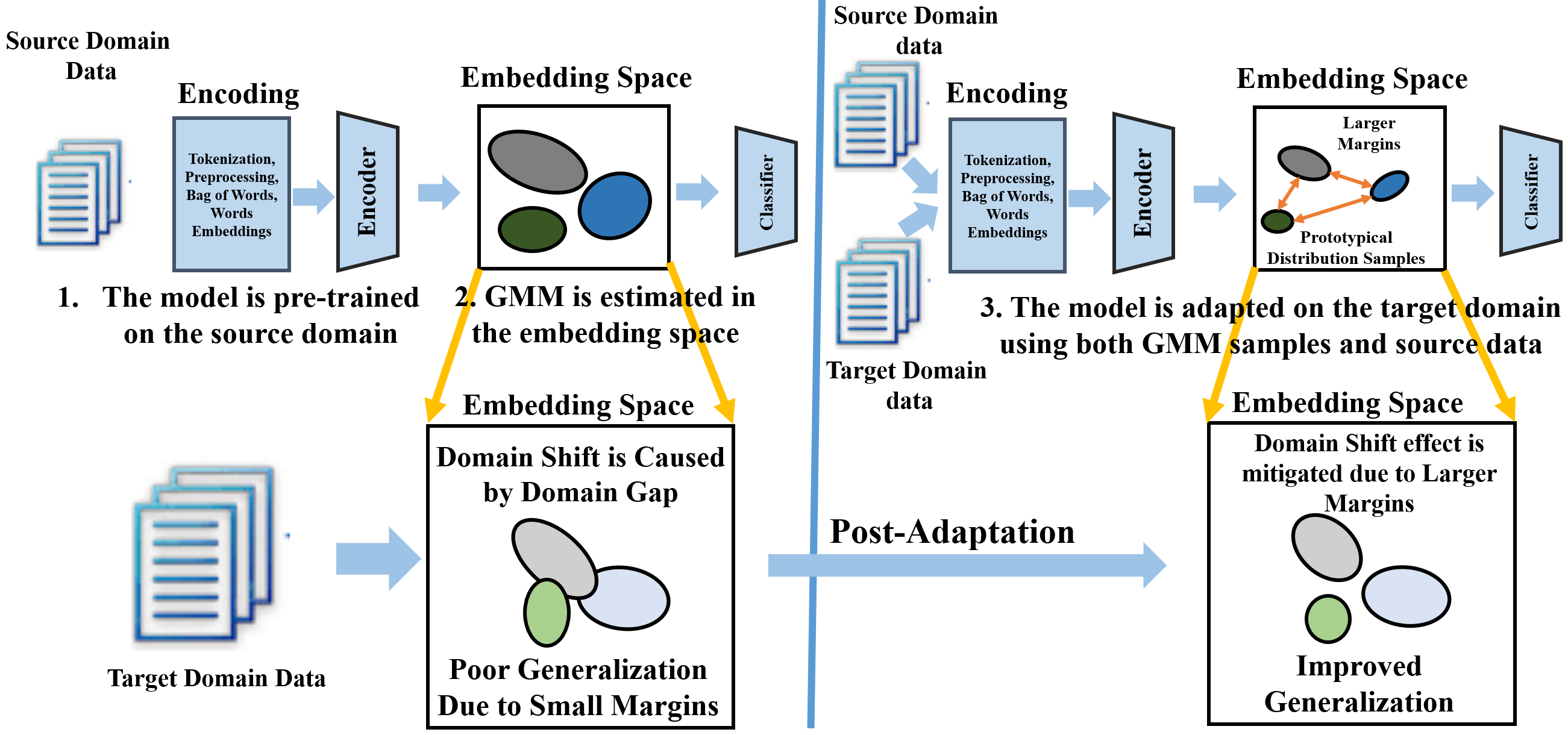
Figure 1: Architecture of the proposed cross-domain sentiment analysis framework. Left: separable clusters are formed in the embedding space after initial supervised model training in the source domain and then the multimodal distribution is estimated as a GMM. Right: random samples from the GMM with high-confident labels are used to generate a pseudo-dataset. The pseudo-dataset helps to induce larger margins between the classes to mitigate domain shift in the target domain.

Consider two sentiment analysis problems in a source domain $\mathcal{S}$ with an annotated dataset $D_{\mathcal{S}}=(\bm{X}_{\mathcal{S}},\bm{Y}_{\mathcal{S}})$, where $\bm{X}_{\mathcal{S}}=[\bm{x}_{1}^{s},\ldots,\bm{x}_{N}^{s}]\in\mathcal{X}\subset\mathbb{R}^{d\times N}$ and $\bm{Y}_{\mathcal{S}}=[\bm{y}^{s}_{1},...,\bm{y}^{s}_{N}]\in\mathcal{Y}\subset\mathbb{R}^{k\times N}$, and a target domain $\mathcal{T}$ with an unannotated dataset $D_{\mathcal{T}}=(\bm{X}_{\mathcal{S}})$, where $\bm{X}_{\mathcal{T}}=[\bm{x}_{1}^{t},\ldots,\bm{x}_{N}^{t}]\in\mathcal{X}\subset\mathbb{R}^{d\times M}$. The real-valued feature vectors $\bm{X}_{\mathcal{S}}$ and $\bm{X}_{\mathcal{T}}$ are obtained after pre-processing the input text data using common NLP methods, e.g., bag of words or word2vec. We consider that both domains share the same type of sentiments and hence the one-hot labels $\bm{y}_{i}^{s}$ encode $k$ sentiment types, e.g., negative or positive in binary sentiment analysis. Additionally, we assume that the source and the target feature data points are drawn independently and identically distributed from the domain-specific distributions $\bm{x}_{i}^{s}\sim p_{S}(\bm{x})$ and $\bm{x}_{i}^{t}\sim p_{T}(\bm{x})$. There is a gap between these distributions, i.e., $p_{T}(\bm{x})\neq p_{S}(\bm{x})$, which makes them distinct.

Given a family of parametric functions $f_{\theta}:\mathbb{R}^{d}\rightarrow\mathcal{Y}$, e.g., deep neural networks with learnable weights $\theta$, and considering an ideal labeling function $f(\cdot)$, e.g., $\forall(\bm{x},\bm{y}):\bm{y}=f(\bm{x})$, the goal is to search for the optimal predictor $f_{\theta^{*}}(\cdot)$ in this family for the target domain. This model should have minimal expected error, i.e., $\theta^{*}=\arg\min_{\theta}\{e_{\theta}\}=\arg\min_{\theta}\{\mathbb{E}_{\bm{x}^{t}\sim p_{T}(\bm{x})}(\mathcal{L}(f(\bm{x}^{t}),f_{\theta}(\bm{x}^{t}))\}$, where $\mathcal{L}(\cdot)$ is a proper loss function and $\mathbb{E}(\cdot)$ denotes the expectation operator. Since the target domain data is unlabeled, the naive approach is to estimate the optimal model using the standard empirical risk minimization (ERM) in the source domain:

$$\begin{split}\hat{\theta}&=\arg\min_{\theta}\{\hat{e}_{\theta}(\bm{X}_{\mathcal{S}},\bm{Y}_{\mathcal{S}},\mathcal{L})\}\\ &=\arg\min_{\theta}\{\frac{1}{N}\sum_{i}\mathcal{L}(f_{\theta}(\bm{x}_{i}^{s}),\bm{y}_{i}^{s})\}.\end{split}$$ (1)

Given a large enough labeled data points in the source domain, ERM model generalizes well in the source domain. The source-trained model may also perform much better than chance in the target domain, given cross-domain knowledge transfer. However, its performance will degrade in the target domain compared to its performance in the source domain because of existing distributional discrepancy between the two domains, since $p_{S}\neq p_{T}$. Our goal is to benefit from the encoded information in the unlabeled target domain data points and adapt the source-trained classifier $f_{\hat{\theta}}$ to generalize in the target domain. We use the common approach of reducing the domain gap across the domains by mapping data into a shared embedding space.

We consider that the predictor model $f_{\theta}(\cdot)$ can be decomposed into a deep encoder subnetwork $\phi_{\bm{v}}(\cdot):\mathcal{X}\rightarrow\mathcal{Z}\subset\mathbb{R}^{p}$ and a classifier subnetwork $h_{\bm{w}}(\cdot):\mathcal{Z}\rightarrow\mathcal{Y}$ such that $f_{\theta}=h_{\bm{w}}\circ\phi_{\bm{v}}$, where $\theta=(\bm{w},\bm{v})$. Here, $\mathcal{Z}$ is an embedding space which is modeled by the encoder responses at its output. We assume that the classes have become separable for the source domain in this space after an initial training phase on the source domain (see Figure 1, left). If we can adapt the source-trained encoder network such that the two domains share similar distributions $\mathcal{Z}$, i.e., $\phi(p_{\mathcal{S}})(\cdot)\approx\phi(p_{\mathcal{T}})(\cdot)$, the embedding space would become domain-agnostic. As a result, the source-trained classifier network will generalize with similar performance in the target domain. A number of prior cross-domain sentiment analysis algorithms use this strategy, select a proper probability distribution metric to compute the distance between the distributions $\phi(p_{\mathcal{S}}(\bm{x}^{s}))$ and $\phi(p_{\mathcal{T}}(\bm{x}^{t}))$, and then train the encoder network to align the domains via minimizing this distance:

$$\begin{split}&\hat{\bm{v}},\hat{\bm{w}}=\arg\min_{\bm{v},\bm{w}}\frac{1}{N}\sum_{i=1}^{N}\mathcal{L}\big{(}h_{\bm{w}}(\phi_{\bm{v}}(\bm{x}_{i}^{s})),\bm{y}_{i}^{s}\big{)}\\ &+\lambda D\big{(}\phi_{\bm{v}}(p_{\mathcal{S}}(\bm{X}_{\mathcal{T}})),\phi_{\bm{v}}(p_{\mathcal{T}}(\bm{X}_{\mathcal{T}}))\big{)},\end{split}$$ (2)

where $D(\cdot,\cdot)$ denotes a probability metric to measure the domain discrepancy and $\lambda$ is a trade-off parameter between the source ERM and the domain alignment term. We base our work on this general approach and use SWD Lee et al. (2019) to compute $D(\cdot,\cdot)$ in (2). Using SWD has three advantages. First, SWD can be computed efficiently compared to WD based on a closed form solution of WD distance in 2D. Second, SWD can be computed using the empirical samples that are drawn from the two distributions. Finally, SWD possesses a non-vanishing gradient even when the support of the two distributions do not overlap Bonnotte (2013); Lee et al. (2019). Hence SWD is suitable for solving deep learning problems which are normally handled using first-order gradient-based optimization techniques, e.g., Adam or SGD Stan and Rostami (2021a).

While methods based on variations of Eq. (2) are effective to reduce the domain gap to some extent, our goal is to improve upon the baseline obtained by Eq. (2) by introducing a loss term that increases the margins between classes in the source domain (check the embedding space in Figure 1, right, for having a better intuition). By doing so, our goal is to mitigate the negative effect of domain shift.

4 Increasing Intraclass Margins

Algorithm 1 $\mathrm{SAIM}^{2}\left(\lambda,\tau\right)$

1:Initial Training:

2:  Input: source dataset $\mathcal{D}_{\mathcal{S}}=(\bm{X}_{\mathcal{S}},\bm{Y}_{\mathcal{S}})$,

3:    Training on the Source Domain:

4:     $\hat{\theta}_{0}=(\hat{\bm{w}}_{0},\hat{\bm{v}}_{0})$

5:        $=\arg\min_{\theta}\sum_{i}\mathcal{L}(f_{\theta}(\bm{x}_{i}^{s}),\bm{y}_{i}^{s})$

6:   GMM Distribution Estimation:

7:     Use (4) and estimate $\alpha_{j},\bm{\mu}_{j},$ $\Sigma_{j}$

8:Model Adaptation:

9:   Input: target dataset $\mathcal{D}_{\mathcal{T}}=\bm{X}_{\mathcal{T}}$

10:   Pseudo-Dataset Generation:

11:     $\mathcal{\hat{D}}_{\mathcal{P}}=(\textbf{Z}_{\mathcal{P}},\textbf{Y}_{\mathcal{P}})=$

12:       $([\bm{z}_{1}^{p},\ldots,\bm{z}_{N}^{p}],[\bm{y}_{1}^{p},\ldots,\bm{y}_{N}^{p}])$, where:

13:               $\bm{z}_{i}^{p}\sim\hat{p}_{J}(\bm{z}),1\leq i\leq N_{p}$

14:               $\bm{y}_{i}^{p}=\arg\max_{j}\{h_{\hat{\bm{w}}_{0}}(\bm{z}_{i}^{p})\},$

15:                    $\max\{h_{\hat{\bm{w}}_{0}}(\bm{z}_{i}^{p})\}>\tau$

16:for $itr=1,\ldots,ITR$  do

17:     draw data batches from $\mathcal{D}_{\mathcal{S}}$, $\mathcal{D}_{\mathcal{T}}$, and $\mathcal{D}_{\mathcal{P}}$

18:     Update the model by solving (6)

19:end for

Our idea for increasing margins between the classes is based on learning an intermediate parametric distribution in the embedding space. We demonstrate that this distribution can be used to induce larger margins between the classes. To this end, we consider that the classifier subnetwork consists of a softmax layer. This means that the classifier should become a maximum a posteriori (MAP) estimator after training to be able to assign a membership probability to a given input feature vector. Under this formulation, the model will generalize in the source domain if after supervised training of the model using the source data, the input distribution is transformed into a multi-modal distribution $p_{J}(\cdot)=\phi_{\bm{v}}(p_{\mathcal{S}})(\cdot)$ with $k$ modes in the embedding space (see Figure 1, left). Each mode of this distribution corresponds to one type of sentiments. The geometric distance between the modes of this distribution corresponds to the margins between classes. If we test the source-trained model in the target domain, the boundaries between class modes will change due to the existence of “domain shift”, i.e., $\phi_{\bm{v}}(p_{\mathcal{T}})(\cdot)\neq\phi_{\bm{v}}(p_{\mathcal{S}})(\cdot)$. Intuitively, as visualized in Figure 1, if we can increase the margins between the class-specific modes in the source domain, domain shift will likely cause less performance degradation Tommasi and Caputo (2013).

We estimate the multimodal distribution in the embedding space as a parametric GMM as follows:

$$p_{J}(\bm{z})=\sum_{j=1}^{k}\alpha_{j}\mathcal{N}(\bm{z}|\bm{\mu}_{j},\bm{\Sigma}_{j}),$$ (3)

where $\bm{\mu}_{j}$ and $\bm{\Sigma}_{j}$ denote the mean and co-variance matrices for each component and $\alpha_{j}$ denotes mixture weights for each component. We solve for these parameters to estimate the multimodal distribution. Note that unlike usual cases in which iterative and time-consuming algorithms such as expectation maximization algorithm need to be used for estimating the GMM parameters, the source domain data points are labeled. As a result, we can estimate $\bm{\mu}_{j}$ and $\bm{\Sigma}_{j}$ for each component independently using standard MAP estimates. Similarly, the weights $\alpha_{j}$ can be computed by a MAP estimate. Let $\bm{S}_{j}$ denote the support set for class $j$ in the training dataset, i.e., $\bm{S}_{j}=\{(\bm{x}_{i}^{s},\bm{y}_{i}^{s})\in\mathcal{D}_{\mathcal{S}}|\arg\max\bm{y}_{i}^{s}=j\}$. To cancel out outliers, we include only those source samples in the $\bm{S}_{j}$ sets, for which the source-trained model predicts the corresponding labels correctly. The closed-form MAP estimate for the mode parameters is given as:

$$\begin{split}&\hat{\alpha}_{j}=\frac{|\bm{S}_{j}|}{N},\hskip 5.69054pt\hat{\bm{\mu}}_{j}=\sum_{(\bm{x}_{i}^{s},\bm{y}_{i}^{s})\in\bm{S}_{j}}\frac{1}{|\bm{S}_{j}|}\phi_{v}(\bm{x}_{i}^{s}),\hskip 5.69054pt\\ &\hat{\bm{\Sigma}}_{j}=\sum_{(\bm{x}_{i}^{s},\bm{y}_{i}^{s})\in\bm{S}_{j}}\frac{1}{|\bm{S}_{j}|}\big{(}\phi_{v}(\bm{x}_{i}^{s})-\hat{\bm{\mu}}_{j}\big{)}^{\top}\big{(}\phi_{v}(\bm{x}_{i}^{s})-\hat{\bm{\mu}}_{j}\big{)}.\end{split}$$ (4)

Computations in Eq. (4) can be done efficiently. For a complexity analysis, please refer to the Appendix. Our idea is to use this multimodal GMM distributional estimate to induce larger margins in the source domain (see Figure 1, right). We update the domain alignment term in (2) to induce larger margins. To this end, we augment the source domain samples in the domain alignment term with samples of a labeled pseudo-dataset $\mathcal{D}_{\mathcal{P}}=(\textbf{Z}_{\mathcal{P}},\textbf{Y}_{\mathcal{P}})$ that we generate using the GMM estimate, where $\bm{Z}_{\mathcal{P}}=[\bm{z}_{1}^{p},\ldots,\bm{z}_{N_{p}}^{p}]\in\mathbb{R}^{p\times N_{p}},\bm{Y}_{\mathcal{P}}=[\bm{y}^{p}_{1},...,\bm{y}^{p}_{N_{p}}]\in\mathbb{R}^{k\times N_{p}}$. This pseudo-dataset is generated using the the GMM distribution. We draw samples from the GMM distributional estimate $\bm{z}_{i}^{p}\sim\hat{p}_{J}(\bm{z})$ for this purpose. To induce larger margins between classes, we feed the initial drawn samples into the classifier network and check the confidence level of the classifier about its predictions for these randomly drawn samples. We set a confidence threshold $\tau\approx 1$ level and only select a subset of the drawn samples for which the confidence level of the classifier is more than $\tau$:

$$\begin{split}&(\bm{z}_{i}^{p},\bm{y}^{p}_{i})\in\mathcal{D}_{\mathcal{P}}\hskip 5.69054pt\text{if:}\hskip 5.69054pt\bm{z}_{i}^{p}\sim\hat{p}_{J}(\bm{z})\hskip 5.69054pt\text{and}\hskip 5.69054pt\\ &\max\{h(\bm{z}_{i}^{p})\}>\tau\hskip 5.69054pt\text{and}\hskip 5.69054pt\bm{y}^{p}_{i}=\arg\max_{i}\{h(\bm{z}_{i}^{p})\}.\end{split}$$ (5)

Given the GMM distributional form, selection of samples based on the threshold $\tau$ means that we include GMM samples that are close to the class-specific mode means $\mu_{i}$ (see Figure 1). In other words, the margins between the clusters in the source domain increase if we use the generated pseudo-dataset for domain alignment. Hence, we update Eq. (2) and solve the following problem:

$$\begin{split}&\hat{\bm{v}},\hat{\bm{w}}=\arg\min_{\bm{v},\bm{w}}\Big{\{}\frac{1}{N}\sum_{i=1}^{N}\mathcal{L}\big{(}h_{\bm{w}}(\phi_{\bm{w}}(\bm{x}_{i}^{s})),\bm{y}_{i}^{s}\big{)}\\ &+\frac{1}{N_{p}}\sum_{i=1}^{N_{p}}\mathcal{L}\big{(}h_{\bm{w}}(\bm{z}_{i}^{s}),\bm{y}_{i}^{s}\big{)}+\lambda\hat{D}\big{(}\phi_{\bm{v}}(\bm{X}_{\mathcal{T}}),\bm{X}_{\mathcal{P}}))\Big{)}\\ &+\lambda\hat{D}\big{(}\phi_{\bm{v}}(\bm{X}_{\mathcal{S}}),\bm{X}_{\mathcal{P}}\big{)}\big{\}},\end{split}$$ (6)

The first and the second terms in (6) are ERM terms for the source dataset and the generated pseudo-dataset in the embedding space to guarantee that the classifier continues to generalize well in the source domain after adaptation. The third and the fourth terms are empirical SWD losses that align the source and the target domain distributions using the pseudo-dataset which as we describe induces larger margins. The hope is that as visualized in Figure 1, these terms can reduce the effect of domain shift. Our proposed solution, named Sentiment Analysis using Increased-Margin Models (SAIM²), is presented and visualized in Algorithm 1 and Figure 1.

5 Theoretical Analysis

Following a standard PAC-learning framework Shalev-Shwartz and Ben-David (2014), we prove that Algorithm 1 minimizes an upperbound for the target domain expected error. Consider that the hypothesis class in a PAC-learning setting is the family of classifier sub-networks $\mathcal{H}=\{h_{\bm{w}}(\cdot)|h_{\bm{w}}(\cdot):\mathcal{Z}\rightarrow\mathbb{R}^{k},\bm{v}\in\mathbb{R}^{V}\}$, where $V$ denotes the number of learnable parameters. We represent the expected error for a model $h_{\bm{w}}(\cdot)\in\mathcal{H}$ on the source and the target domains by $e_{\mathcal{S}}(\bm{w})$ and $e_{\mathcal{T}}(\bm{w})$, respectively. Given the source and the target datasets, we can represent the empirical source and target distributions in the embedding space as $\hat{\mu}_{\mathcal{S}}=\frac{1}{N}\sum_{n=1}^{N}\delta(\phi_{\bm{v}}(\bm{x}_{n}^{s}))$ and $\hat{\mu}_{\mathcal{T}}=\frac{1}{M}\sum_{m=1}^{M}\delta(\phi_{\bm{v}}(\bm{x}_{m}^{t}))$. Similarly, we can build an empirical distribution for the multimodal distribution $\hat{\mu}_{\mathcal{P}}=\frac{1}{N_{p}}\sum_{q=1}^{N_{p}}\delta(\bm{z}_{n}^{q})$. In our analysis we also use the notion of joint-optimal model $h_{\mathcal{S},\mathcal{T}}(\cdot)$ in our analysis which is defined as: $\bm{w}^{*}=\arg\min_{\bm{w}}e_{\mathcal{S},\mathcal{T}}=\arg\min_{\bm{w}}\{e_{\mathcal{S}}+e_{\mathcal{T}}\}$ for any given domains $\mathcal{S}$ and $\mathcal{T}$. When we have labeled data in both domains, this is the best model that can be trained using ERM. Existence of a good joint-trained model guarantees that the domains are related, e.g., similar types of sentiment polarities are encoded across the two domains, to make positive knowledge transfer feasible.

Theorem 1: Consider that we use the procedure described in Algorithm 1 for cross-domain sentiment analysis, then the following inequality holds for the target expected error:

$$\begin{split}e_{\mathcal{T}}\leq&e_{\mathcal{S}}+\hat{D}(\hat{\mu}_{\mathcal{S}},\hat{\mu}_{\mathcal{P}})+\hat{D}(\hat{\mu}_{\mathcal{T}},\hat{\mu}_{\mathcal{P}})+(1-\tau)+e_{\mathcal{S},\mathcal{P}}\\ &+\sqrt{\big{(}2\log(\frac{1}{\xi})/\zeta\big{)}}\big{(}\sqrt{\frac{1}{N}}+\sqrt{\frac{1}{M}}+2\sqrt{\frac{1}{N_{p}}}\big{)},\end{split}$$ (7)

where $\xi$ is a constant which depends on the properties of the loss function $\mathcal{L}(\cdot)$.

Proof: the complete proof is included in the Appendix.

Theorem 1 provides an explanation to justify Algorithm 1. We observe that all the terms in the upperbound of the target expected error in the right-hand side of (7) are minimized by $SAIM^{2}$. The source expected error is minimized as the first term in (6). The second and the third terms terms are minimized as the third and fourth terms of (6). The fourth term $1-\tau$ will be small if we set $\tau\approx 1$. The term $e_{\mathcal{S},\mathcal{P}}$ is minimized through the first and the second term of (6). This is highly important as using the pseudo-dataset provides a way to minimize this term. As can be seen in our proof in the Appendix, if we don’t use the pseudo-dataset, this terms is replaced with $e_{\mathcal{S},\mathcal{T}}$ which cannot be minimized directly due to lack of having annotated data in the target domain. The last term in (7) is a constant term that as common in PAC-learning can become negligible states that in order to train a good model if we have access to large enough datasets. Hence all the terms in the upperbound are minimized and if this upperbound is tight, then the process leads to training a good model for the target domain. If the two domain are related, e.g., share the same classes, and also classes become separable in the embedding space, i.e., GMM estimation error for the source domain distribution in the embedding space is small, then the upperbound is going to be likely tight. However, we highlight that possibility of a tight upperbound is a condition for our algorithm to work. This is a common limitation for most parametric learning algorithms.

6 Experimental Validation

Our implemented code is available at https://github.com/mrostami1366.

6.1 Experimental Setup

We have selected the most common setup to perform our experiments for possibility of comparison.

Dataset and preprocessing: Most existing works report performance cross-domain tasks that are defined using the Amazon Reviews benchmark dataset Blitzer et al. (2007). The dataset is built using Amazon product reviews from four product domains: Books (B), DVD (D), Electronics (E), and Kitchen (K) appliances. Each review is considered to have positive (higher than 3 stars) or negative (3 stars or lower) sentiment. Following the most common setup in the literature, we encode each review in a 5000 dimensional or 30000 dimensional tf-idf feature vector of bag-of-words unigrams and bigrams to compare our results against the existing benchmarks. Note that using more advanced text embedding methods increases the absolute performance, but we are interested in studying the relative improvement compared to the source-trained model. For this reason, we use these features to have domain gap. Each task consists of 2000 labeled reviews for the source domain and 2000 unlabeled reviews for the target domain, and 2500–5500 examples for testing. We report our performance on the 12 definable cross-domain tasks for this dataset. We report the average prediction accuracy and standard deviation (std) over 10 runs on the target domain testing split for our algorithm.

Baselines: We compare our method against recently developed algorithms. We compare against DSN Bousmalis et al. (2016) CMD Zellinger et al. (2017), ASYM Saito et al. (2018), PBLM Ziser and Reichart (2018), MT-Tri Ruder and Plank (2018), TRL Ziser and Reichart (2019), and TAT Liu et al. (2019). These works are representative of advances in the field based on various approaches. DSN and CMD are similar to $SAIM^{2}$ in that both align distributions in an embedding space. DSN learns shared and domain-specific knowledge for each domain and aligns the shared knowledge using the mean-based maximum mean discrepancy metric. CMD uses the central moment discrepancy metric for domain alignment. ASYM benefits from the idea of pseudo-labeling of the target samples to updated the base model. MT-Tri is based on ASYM but it also benefits from multi-task learning. TRL and PBLM do not use distribution alignment and are based on the pivot based language model. TAT is a recent work that has used adversarial learning successfully for cross-domain sentiment analysis. We provided results by the authors for the tasks in our table. We report std if std is reported in the original paper. All the methods except TAT that uses 30000 dimensional features, use 5000 dimensional features. Note that in the results, the methods are comparable if they use features with the same dimension for fair comparison. We report performance of the source only (SO) model as a lowerbound to demonstrate the effect of adapting the model over this baseline.

Model and optimization setup: We used the benchmark network architecture that is used in the above mentioned works for fair comparison. We used an encoder with one hidden dense layer with 50 nodes with sigmoid activation function. The classifiers consist of a softmax layer with two output nodes. We implemented our method in Keras, used adam optimizer and tuned the learning rate in the source domain. We set $\tau=0.99$ and $\lambda=10^{-2}$. We tuned them based on a brute-force search. We observed empirically that our algorithm is not sensitive to the value of $\lambda$. We ran our code on a cluster equipped with 4 Nvidia Tesla P100-SXM2 GPUs.

Task	B$\rightarrow$D	B$\rightarrow$E	B$\rightarrow$K	D$\rightarrow$B	D$\rightarrow$E	D$\rightarrow$K
SO	81.7 $\pm$ 0.2	74.0 $\pm$ 0.6	76.4 $\pm$ 1.0	74.5 $\pm$ 0.3	75.6 $\pm$ 0.7	79.5 $\pm$ 0.4
DSN	82.8 $\pm$ 0.4	81.9 $\pm$ 0.5	84.4 $\pm$ 0.6	80.1 $\pm$ 1.3	81.4 $\pm$ 1.1	83.3 $\pm$ 0.7
CMD	82.6 $\pm$ 0.3	81.5 $\pm$ 0.6	84.4 $\pm$ 0.3	$\bm{80.7}$ $\pm$ 0.6	82.2 $\pm$ 0.5	84.8 $\pm$ 0.2
ASYM	80.7	79.8	82.5	73.2	77.0	82.5
PBLM	84.2	77.6	82.5	82.5	79.6	83.2
MT-Tri	81.2	78.0	78.8	77.1	81.0	79.5
TRL	82.2	-	82.7	-	-	-
$SAIM^{2}$	$\bm{83.2}$ $\pm$ 0.2	$\bm{83.9}$ $\pm$ 0.3	$\bm{85.}9$ $\pm$ 0.3	80.3 $\pm$ 0.4	$\bm{84.2}$ $\pm$ 0.3	$\bm{87.3}$ $\pm$ 0.2
TAT∗	84.5	80.1	83.6	81.9	81.9	84.0
$SAIM^{2}$∗	86.2 $\pm$ 0.2	85.1 $\pm$ 0.2	87.6 $\pm$ 0.2	80.9 $\pm$ 0.5	85.2 $\pm$ 0.2	88.6 $\pm$ 0.2
Task	E$\rightarrow$B	E$\rightarrow$D	E$\rightarrow$K	K$\rightarrow$B	K$\rightarrow$D	K$\rightarrow$E
SO	72.3 $\pm$ 1.5	74.2 $\pm$ 0.6	85.6 $\pm$ 0.6	73.1 $\pm$ 0.1	75.2 $\pm$ 0.7	85.4 $\pm$ 1.0
DSN	75.1 $\pm$ 0.4	77.1 $\pm$ 0.3	87.2 $\pm$ 0.7	76.4 $\pm$ 0.5	78.0 $\pm$ 1.4	86.7 $\pm$ 0.7
CMD	74.9 $\pm$ 0.6	77.4 $\pm$ 0.3	86.4 $\pm$ 0.9	75.8 $\pm$ 0.3	77.7 $\pm$ 0.4	86.7 $\pm$ 0.6
ASYM	73.2	72.9	86.9	72.5	74.9	84.6
PBLM	71.4	75.0	87.8	74.2	$\bm{79.8}$	$\bm{87.1}$
MT-Tri	73.5	75.4	87.2	73.8	77.8	86.0
TRL	-	75.8	-	72.1	-	-
$SAIM^{2}$	$\bm{78.6}$ $\pm$ 0.4	$\bm{79.7}$ $\pm$ 0.2	$\bm{89.2}$ $\pm$ 0.2	$\bm{76.7}$ $\pm$ 0.4	79.1 $\pm$ 0.4	87.0 $\pm$ 0.1
TAT∗	83.2	77.9	90.0	75.8	77.7	88.2
$SAIM^{2}$∗	78.8 $\pm$ 0.3	78.9 $\pm$ 0.3	90.1 $\pm$ 0.2	78.1 $\pm$ 0.2	78.8 $\pm$ 0.4	88.1 $\pm$ 0.1

Table 1: Classification accuracy for the cross-domain sentiment analysis tasks for Amazon Reviews dataset. In this table, ^∗ denotes methods that use $30000$ dimensional tf-idf feature vectors.

6.2 Comparative Results

Our results are reported in Table 1. In this table, bold font denotes best performance among the methods that use 5000 dimensional features. We see that $SAIM^{2}$ algorithm performs reasonably well and in most cases leads to the best performance. Note that this is not unexpected as none of the methods has the best performance across all tasks. We observe from this table that overall the methods DSN and CMD which are based on aligning the source and target distributions- which are more similar to our algorithm- have relatively similar performances. This observation suggests that we should not expect considerable performance boost if we simply align the distributions by designing a new alignment loss function. This means that outperformance of $SAIM^{2}$ compared to these methods stems from inducing larger margins. We verify this intuition in our ablative study. We also observe that increasing the dimensional of tf-idf features to 30000 leads to performance boost which is probably the reason behind good performance of TAT. Hence, we need to use the same dimension for features for fair comparison among the methods.

To provide an empirical exploration to validate the intuition we used for our rationale, we have used UMAP McInnes et al. (2018) to reduce the dimension of the data representations in the 50D embedding space to two for the purpose of 2D visualization. Figure 2 visualizes the testing splits of the source domain before model adaptation, the testing splits of the target domain before and after model adaptation, and finally random samples drawn from the estimated GMM distribution for the D$\rightarrow$K task. Each point represents one data point and each color represents one of the sentiments. Observing Figure 2(a) and Figure 2(b), we conclude that the estimated GMM distribution approximates the source domain distribution reasonably well and at the same time, a margin between the classes in the boundary region is observable. Figure 2(c) visualizes the target domain samples prior to model adaptation. As expected, we observe that domain gap has caused less separations between the classes, as also evident from SO performance in Table 1. Figure 2(d) visualizes the target domain samples after adaptation using $SAIM^{2}$ algorithm. Comparing Figure 2(d) with Figure 2(c) and Figure 2(a), we see that the classes have become more separated. Also, careful comparison of Figure 2(d) and Figure 2(b) reveals $SAIM^{2}$ algorithm has led to a bias in the target domain to move the data points further from the boundary. These visualizations serve as an empirical verification for our theoretical analysis.

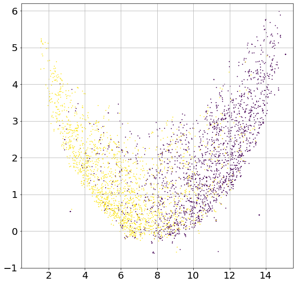
(a) Source

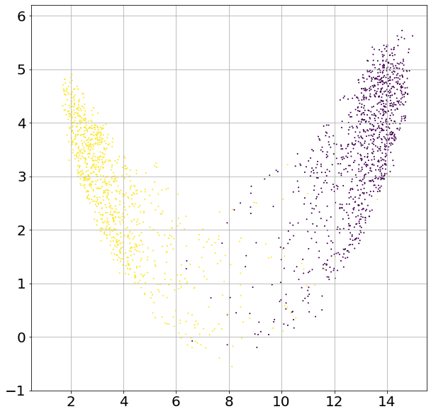
(b) GMM. Dist. Samples

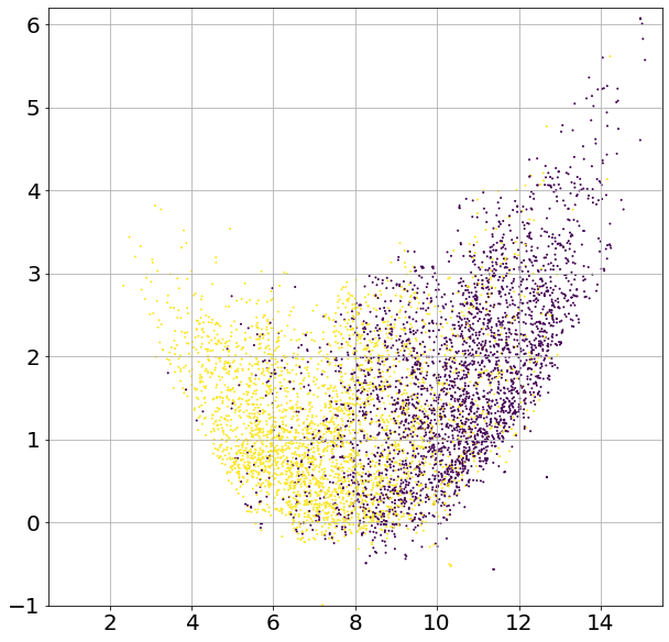
(c) Target: Pre-Adapt.

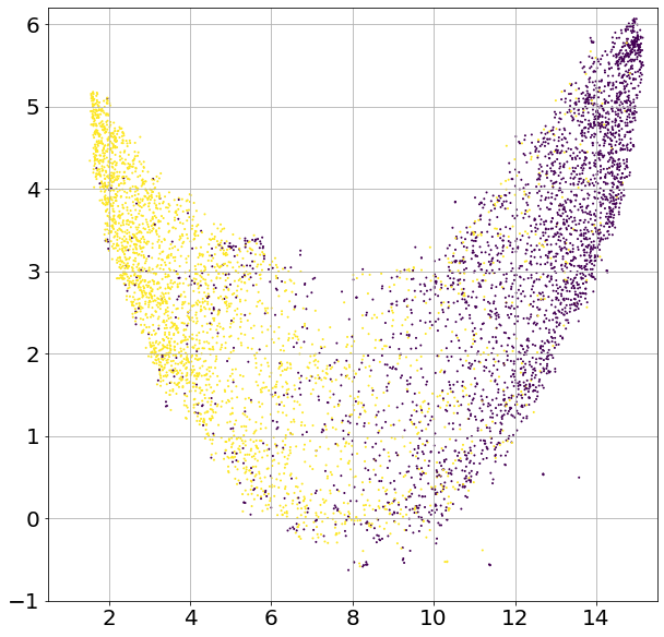
(d) Target: Post-Adapt.

Figure 2: UMAP visualization for the D$\rightarrow$K task: (a) the source domain testing split, (b) the GMM distribution samples, (c) the target domain testing split pre- and (d) post-adaptation. (Best viewed in color).

6.3 Effect of Data Imbalance on Performance

In practical setting, the label distribution for the target domain training dataset cannot be enforced to be balanced due to absence of labels. To study the effect of label imbalance using a controlled experiment, we synthetically design an imbalanced dataset using the Amazon dataset. We designed two experiments, where the target domain datasets has the 90/10 and 80/20 ratios of imbalance between the two classes, respectively. We have provided domain adaptation results using for these two imbalanced scenarios in Table 2. We can see that performance of our algorithm has degraded slightly but our algorithm has been robust to a large extent with respect to label imbalance.

Task	B$\rightarrow$D	B$\rightarrow$E	B$\rightarrow$K	D$\rightarrow$B	D$\rightarrow$E	D$\rightarrow$K
$80/20$	82.8 $\pm$ 0.3	83.2 $\pm$ 0.5	85.5 $\pm$ 0.3	78.7 $\pm$ 0.2	83.3 $\pm$ 0.2	86.8 $\pm$ 0.2
$90/10$	82.9 $\pm$ 0.5	83.4 $\pm$ 0.3	85.8 $\pm$ 0.2	78.5 $\pm$ 0.4	83.3 $\pm$ 0.4	86.8 $\pm$ 0.3
Task	E$\rightarrow$B	E$\rightarrow$D	E$\rightarrow$K	K$\rightarrow$B	K$\rightarrow$D	K$\rightarrow$E
$80/20$	78.7 $\pm$ 0.2	78.5 $\pm$ 0.5	88.6 $\pm$ 0.1	76.3 $\pm$ 0.6	77.9 $\pm$ 0.4	86.6 $\pm$ 0.1
$90/10$	78.7 $\pm$ 0.2	78.0 $\pm$ 0.4	88.0 $\pm$ 0.2	76.5 $\pm$ 0.5	77.3 $\pm$ 0.3	86.7 $\pm$ 0.2

Table 2: Effect of label-imbalance on performance.

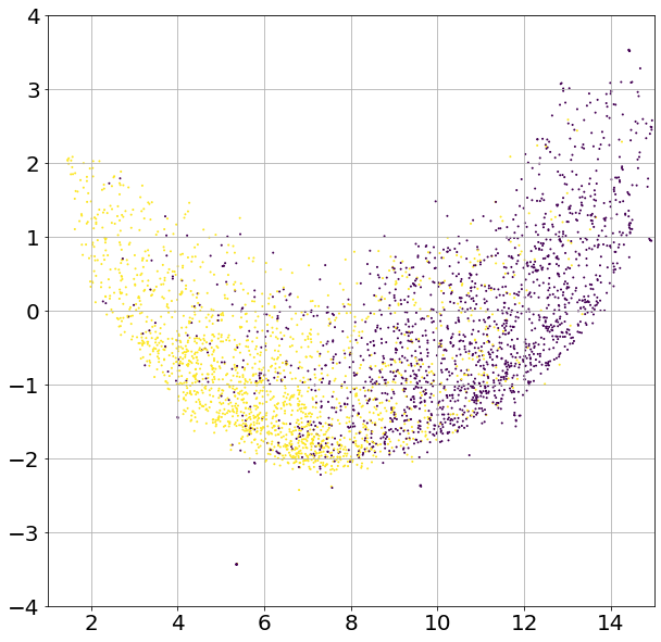
(a) Source

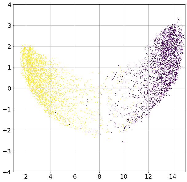
(b) GMM Dist. Samples

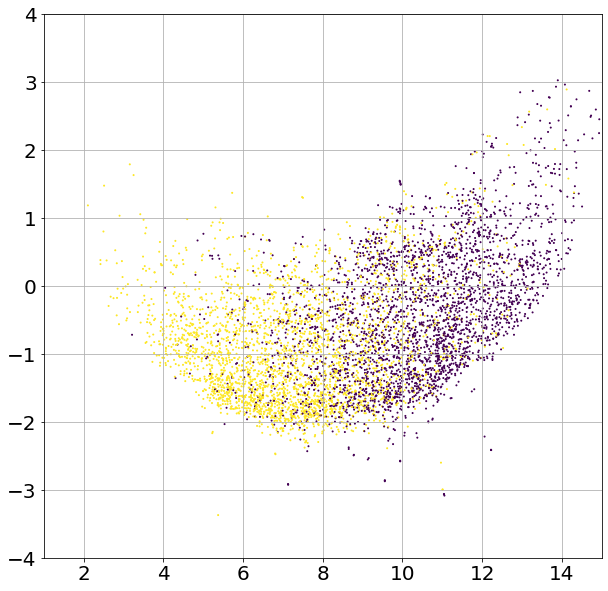
(c) Target: Pre-Adapt.

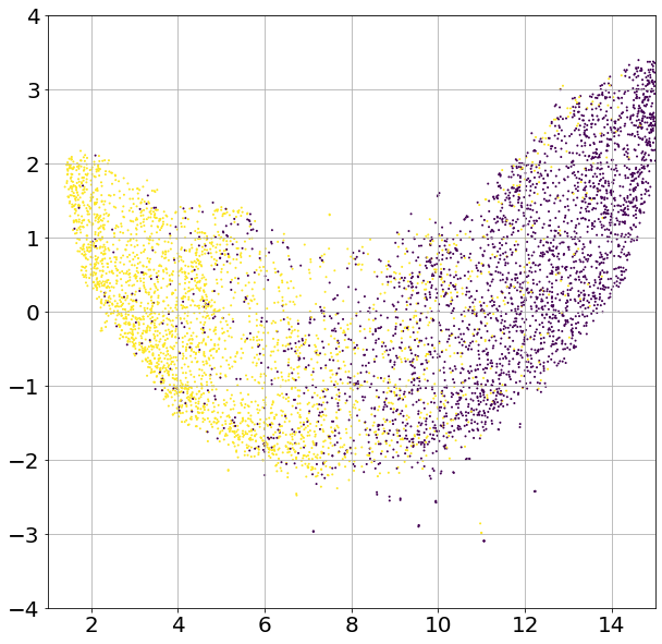
(d) Target: Post-Adapt.

Figure 3: UMAP visualization for the task D$\rightarrow$K task in the imbalanced regime of $90/10$: (a) the source domain testing split, (b) the GMM distribution samples, (c) the target domain testing split pre-, and (d) post-domain adaptation. (Best viewed in color).

For sanity check, we have presented the UMAP visualization for the testing split of the task D$\rightarrow$K for the scenario $90/10$ in Figure 3. Observations in Figure 3 match what we reported in Table 2, confirming that our algorithm does require a balanced dataset imbalanced is practically beneficial.

6.4 Ablation Studies

First note that the source only (SO) model result, which is trained using (1), already serves as a basic ablative study to verify the effect of domain alignment. Improvement over this baseline demonstrates effect of domain adaptation on performance.

In Table 3, we have provided an additional ablative studies. We have reported result of alignment only (AO) model adaptation based on (2). The AO model does not benefit from the margins that $SAIM^{2}$ algorithm induces between the classes. Comparing AO results with Table 1, we can conclude that the effect of increased margins is important in our performance. Compared to other cross-domain sentiment analysis methods, the performance boost for our algorithm stems from inducing large margins. This suggests that researchers may check to investigate secondary techniques for domain adaptation in NLP domains, in addition to probability distribution alignment.

Finally, we have studied the effect of the value of the confidence parameter on performance. In Figure 4, we have visualized the performance of our algorithm for the task $B\rightarrow D$ when $\tau$ is varied in the interval $[0,0.99]$. When $\tau=0$, the samples are not necessarily confident samples. We observe that as we increase the value of $\tau$, the performance increases as a result of inducing larger margins. For values $\tau>0.8$, the performance has less variance which suggests robustness of performance if $\tau\approx 1$. These empirical observations about $\tau$ accord with our theoretical result, stated in the upperbound (7).

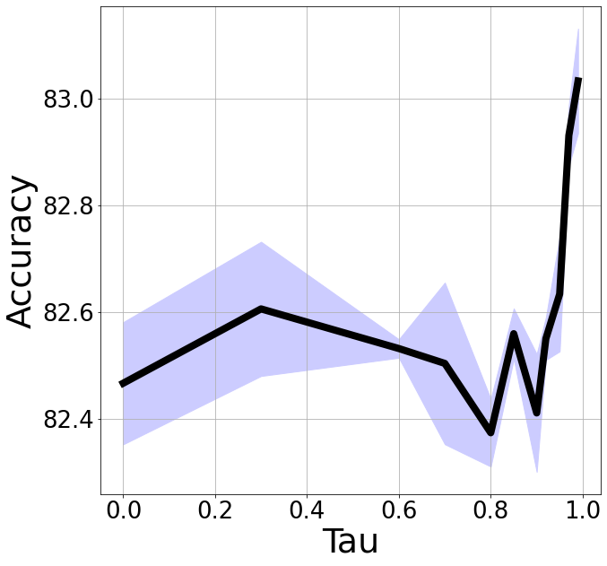
Figure 4: Effect of $\tau$ on performance.

Table 3: Performance for AO.

Task	B$\rightarrow$D	B$\rightarrow$E	B$\rightarrow$K
	81.9 $\pm$ 0.5	80.9 $\pm$ 0.8	83.2 $\pm$ 0.8
Task	D$\rightarrow$B	D$\rightarrow$E	D$\rightarrow$K
	74.0 $\pm$ 0.9	80.9 $\pm$ 0.7	83.4 $\pm$ 0.6
Task	E$\rightarrow$B	E$\rightarrow$D	E$\rightarrow$K
	74.1 $\pm$ 0.6	74.0 $\pm$ 0.3	87.8 $\pm$ 0.9
Task	D$\rightarrow$B	D$\rightarrow$E	D$\rightarrow$K
	74.1 $\pm$ 0.6	74.0 $\pm$ 0.3	87.8 $\pm$ 0.9

7 Conclusions

We developed a method for cross-domain sentiment analysis based on aligning two domain-specific distributions in a shared embedding space and inducing larger margins between the classes in the source domain using an intermediate multi-modal GMM distribution. We theoretically justified our approach. Our experiments demonstrate that our algorithm is effective. A future research direction is to address cross-domain sentiment analysis when different types of sentiments exists in two domains.

Appendix A Proof of Theorem 1

We use the following theorem by Redko et al. Redko and Sebban (2017) and a result by Bolley Bolley et al. (2007) on convergence of the empirical distribution to the true distribution in terms of the WD distance in our proof.

Theorem 2 (Redko et al. Redko and Sebban (2017)): Under the assumptions described in our framework, assume that a model is trained on the source domain, then for any $d^{\prime}>d$ and $\zeta<\sqrt{2}$, there exists a constant number $N_{0}$ depending on $d^{\prime}$ such that for any $\bm{x}_{i}>0$ and $\min(N,M)\geq\max(\bm{x}i^{-(d^{\prime}+2),1})$ with probability at least $1-\bm{x}_{i}$, the following holds:

$$\begin{split}e_{\mathcal{T}}\leq&e_{\mathcal{S}}+W(\hat{\mu}_{\mathcal{T}},\hat{\mu}_{\mathcal{S}})+e_{\mathcal{S},\mathcal{T}}\\ &+\sqrt{\big{(}2\log(\frac{1}{\bm{x}_{i}})/\zeta\big{)}}\big{(}\sqrt{\frac{1}{N}}+\sqrt{\frac{1}{M}}\big{)}.\end{split}$$ (8)

Theorem 2 provides an upperbound for the performance of a source-trained model in the target domain Redko et al. Redko and Sebban (2017) prove Theorem 2 for a binary classification setting. We also provide our proof in this case but it can be extended.

The second term in Eq. (8) demonstrates the effect of domain shift on the performance of a source-trained model in a target domain. When the distance between the two distributions is significant, this term will be large and hence the upperbound in Eq. (8) will be loose which means potential performance degradation. Our algorithm mitigates domain gap because this term is minimized by minimization of the second and the third terms in Theorem 1.

Theorem 1 : Consider that we the procedure described in Algorithm 1 for cross-domain sentiment analysis, then the following inequality holds for the target expected error:

$$\begin{split}e_{\mathcal{T}}\leq&e_{\mathcal{S}}+\hat{D}(\hat{\mu}_{\mathcal{S}},\hat{\mu}_{\mathcal{P}})+\hat{D}(\hat{\mu}_{\mathcal{T}},\hat{\mu}_{\mathcal{P}})+(1-\tau)\\ &+e_{\mathcal{S},\mathcal{P}}+\sqrt{\big{(}2\log(\frac{1}{\bm{x}_{i}})/\zeta\big{)}}\big{(}\sqrt{\frac{1}{N}}+\sqrt{\frac{1}{M}}+2\sqrt{\frac{1}{N_{p}}}\big{)},\end{split}$$ (9)

where $\bm{x}_{i}$ is a constant which depends on $\mathcal{L}(\cdot)$ and $e_{C}^{\prime}(\bm{w}^{*})$ denotes the expected risk of the optimally joint trained model when used on both the source domain and the pseudo-dataset.

Proof: Due to the construction of the pseudo-dataset, the probability that the predicted labels for the pseudo-data points to be false is equal to $1-\tau$. Let:

$$\begin{split}&|\mathcal{L}(h_{\bm{w}_{0}}(\bm{z}^{p}_{i}),\bm{y}^{p}_{i})-\mathcal{L}(h_{\bm{w}_{0}}(\bm{z}^{p}_{i}),\hat{\bm{y}}_{i}^{p})|=\\ &\begin{cases}0,&\text{if $\bm{y}^{t}_{i}=\hat{\bm{y}}_{i}^{t}$}.\\ 1,&\text{otherwise}.\end{cases}\end{split}$$ (10)

We use Jensen’s inequality and take expectation on both sides of (10) to deduce:

$$\begin{split}|e_{\mathcal{P}}-e_{\mathcal{T}}|\leq&\mathbb{E}\big{(}|\mathcal{L}(h_{\bm{w}_{0}}(\bm{z}^{p}_{i}),\bm{y}^{p}_{i})-\mathcal{L}(h_{\bm{w}_{0}}(\bm{z}^{p}_{i}),\hat{\bm{y}}_{i}^{p})|\big{)}\\ &\leq(1-\tau).\end{split}$$ (11)

Applying  (11) in the below, deduce:

$$\begin{split}&e_{\mathcal{S}}+e_{\mathcal{T}}=e_{\mathcal{S}}+e_{\mathcal{T}}+e_{\mathcal{P}}-e_{\mathcal{P}}\leq\\ &e_{\mathcal{S}}+e_{\mathcal{P}}+|e_{\mathcal{T}}-e_{\mathcal{P}}|\leq e_{\mathcal{S}}+e_{\mathcal{P}}+(1-\tau).\end{split}$$ (12)

Taking infimum on both sides of  (12), we deduce:

$$\begin{split}e_{\mathcal{S},\mathcal{T}}\leq e_{\mathcal{S},\mathcal{P}}+(1-\tau).\end{split}$$ (13)

Now by considering Theorem 2 for the two domains $\mathcal{S}$ and $\mathcal{T}$ and then using  (13) in (8), we can conclude:

$$\begin{split}e_{\mathcal{T}}\leq&e_{\mathcal{S}}+D(\hat{\mu}_{\mathcal{T}},\hat{\mu}_{\mathcal{S}})+e_{\mathcal{S},\mathcal{P}}+(1-\tau)\\ &+\sqrt{\big{(}2\log(\frac{1}{\bm{x}_{i}})/\zeta\big{)}}\big{(}\sqrt{\frac{1}{N}}+\sqrt{\frac{1}{M}}\big{)}.\end{split}$$ (14)

Now using the triangular inequality on the metrics we can deduce:

$$\begin{split}&D(\hat{\mu}_{\mathcal{T}},\hat{\mu}_{\mathcal{S}})\leq D(\hat{\mu}_{\mathcal{T}},\mu_{\mathcal{P}})+D(\hat{\mu}_{\mathcal{S}},\mu_{\mathcal{P}})\\ &\leq D(\hat{\mu}_{\mathcal{T}},\hat{\mu}_{\mathcal{P}})+D(\hat{\mu}_{\mathcal{S}},\hat{\mu}_{\mathcal{P}})+2D(\hat{\mu}_{\mathcal{P}},\mu_{\mathcal{P}}).\end{split}$$ (15)

Now we replace the term $D(\hat{\mu}_{\mathcal{P}},\mu_{\mathcal{P}})$ with its empirical counterpart using Theorem 1.1 in the work by  Bolley et al. (2007).

Theorem 3 (Theorem 1.1 by Bolley et al. Bolley et al. (2007)): consider that $p(\cdot)\in\mathcal{P}(\mathcal{Z})$ and $\int_{\mathcal{Z}}\exp{(\alpha\|\bm{x}\|^{2}_{2})}dp(\bm{x})<\infty$ for some $\alpha>0$. Let $\hat{p}(\bm{x})=\frac{1}{N}\sum_{i}\delta(\bm{x}_{i})$ denote the empirical distribution that is built from the samples $\{\bm{x}_{i}\}_{i=1}^{N}$ that are drawn i.i.d from $\bm{x}_{i}\sim p(\bm{x})$. Then for any $d^{\prime}>d$ and $\bm{x}_{i}<\sqrt{2}$, there exists $N_{0}$ such that for any $\epsilon>0$ and $N\geq N_{o}\max(1,\epsilon^{-(d^{\prime}+2)})$, we have:

$$\begin{split}P(W(p,\hat{p})>\epsilon)\leq\exp(-\frac{-\bm{x}_{i}}{2}N\epsilon^{2}),\end{split}$$ (16)

where $W$ denotes the WD distance. This relation measures the distance between the empirical distribution and the true distribution, expressed in the WD distance.

Applying  (15) and  (16) on  (14) concludes Theorem 2 as stated:

$$\begin{split}e_{\mathcal{T}}\leq&e_{\mathcal{S}}+D(\hat{\mu}_{\mathcal{S}},\hat{\mu}_{\mathcal{P}})+D(\hat{\mu}_{\mathcal{T}},\hat{\mu}_{\mathcal{P}})+(1-\tau)+e_{\mathcal{S},\mathcal{P}}+\\ &\sqrt{\big{(}2\log(\frac{1}{\bm{x}_{i}})/\zeta\big{)}}\big{(}\sqrt{\frac{1}{N}}+\sqrt{\frac{1}{M}}+2\sqrt{\frac{1}{N_{p}}}\big{)},\end{split}$$ (17)

Appendix B Complexity analysis for GMM estimation

Estimating a GMM distribution usually is a computationally expensive tasks. The major reason is that normally the data points are unlabeled. This would necessitate relying on iterative algorithms such expectation maximization (EM) algorithm Moon (1996). Preforming iterative E and M steps until convergence leads to high computational complexity Roweis (1998). However, estimating the multimodal distribution with a GMM distribution is much simpler in our learning setting. Existence of labels helps us to decouple the Gaussian components and compute the parameters using MAP estimate for each of the mode parameters in one step as follows:

$$\begin{split}&\hat{\alpha}_{j}=\frac{|\bm{S}_{j}|}{N},\hskip 5.69054pt\\ &\hat{\bm{\mu}}_{j}=\sum_{(\bm{x}_{i}^{s},\bm{y}_{i}^{s})\in\bm{S}_{j}}\frac{1}{|\bm{S}_{j}|}\phi_{v}(\bm{x}_{i}^{s}),\hskip 5.69054pt\\ &\hat{\bm{\Sigma}}_{j}=\sum_{(\bm{x}_{i}^{s},\bm{y}_{i}^{s})\in\bm{S}_{j}}\frac{1}{|\bm{S}_{j}|}\big{(}\phi_{v}(\bm{x}_{i}^{s})-\hat{\bm{\mu}}_{j}\big{)}^{\top}\big{(}\phi_{v}(\bm{x}_{i}^{s})-\hat{\bm{\mu}}_{j}\big{)}.\end{split}$$ (18)

Given the above and considering that the source domain data is balanced, complexity of computing $\alpha_{j}$ is $O(N)$ (just checking whether data points $\bm{x}_{i}^{s}$ belong to $\bm{S}_{j}$). Complexity of computing $\bm{\mu}_{j}$ is $O(NF/k)$, where $F$ is the dimension of the embedding space. Complexity of computing the co-variance matrices $\bm{\Sigma}_{j}$ is $O(F(\frac{N}{k})^{2})$. Since, we have $k$ components, the total complexity of computing GMM is $O(\frac{FN^{2}}{k})$. If $O(F)\approx O(k)$, which seems to be a reasonable practical assumption, then the total complexity of computing GMM would be $O(N^{2})$. Given the large number of learnable parameters in most deep neural networks which are more than $N$ for most cases, this complexity is fully dominated by complexity of a single step of backpropagation. Hence, this computing the GMM parameters does not increase the computational complexity for.

References

- Barnes et al. (2018) Jeremy Barnes, Roman Klinger, and Sabine Schulte im Walde. 2018. Projecting embeddings for domain adaption: Joint modeling of sentiment analysis in diverse domains. In Proceedings of Comp. Linguistics, pages 818–830.
- Bhushan Damodaran et al. (2018) Bharath Bhushan Damodaran, Benjamin Kellenberger, Rémi Flamary, Devis Tuia, and Nicolas Courty. 2018. Deepjdot: Deep joint distribution optimal transport for unsupervised domain adaptation. In Proceedings of the European Conference on Computer Vision (ECCV), pages 447–463.
- Blitzer et al. (2007) John Blitzer, Mark Dredze, and Fernando Pereira. 2007. Biographies, bollywood, boom-boxes and blenders: Domain adaptation for sentiment classification. In Proceedings of ACL, pages 440–447.
- Bolley et al. (2007) François Bolley, Arnaud Guillin, and Cédric Villani. 2007. Quantitative concentration inequalities for empirical measures on non-compact spaces. Probability Theory and Related Fields, 137(3-4):541–593.
- Bonnotte (2013) N. Bonnotte. 2013. Unidimensional and evolution methods for optimal transportation. Ph.D. thesis, Paris 11.
- Bousmalis et al. (2016) Konstantinos Bousmalis, George Trigeorgis, Nathan Silberman, Dilip Krishnan, and Dumitru Erhan. 2016. Domain separation networks. In Proceedings of NeurIPS, pages 343–351.
- Courty et al. (2016) Nicolas Courty, Rémi Flamary, Devis Tuia, and Alain Rakotomamonjy. 2016. Optimal transport for domain adaptation. IEEE transactions on pattern analysis and machine intelligence, 39(9):1853–1865.
- Dai et al. (2020) Yong Dai, Jian Liu, Xiancong Ren, and Zenglin Xu. 2020. Adversarial training based multi-source unsupervised domain adaptation for sentiment analysis. In AAAI.
- Du et al. (2020) Chunning Du, Haifeng Sun, Jingyu Wang, Qi Qi, and Jianxin Liao. 2020. Adversarial and domain-aware bert for cross-domain sentiment analysis. In Proceedings of the 58th Annual Meeting of the Association for Computational Linguistics, pages 4019–4028.
- Gong et al. (2020) Chenggong Gong, Jianfei Yu, and Rui Xia. 2020. Unified feature and instance based domain adaptation for end-to-end aspect-based sentiment analysis. In Proceedings of the 2020 Conference on Empirical Methods in Natural Language Processing (EMNLP), pages 7035–7045.
- Goodfellow et al. (2014) Ian Goodfellow, Jean Pouget-Abadie, Mehdi Mirza, Bing Xu, David Warde-Farley, Sherjil Ozair, Aaron Courville, and Yoshua Bengio. 2014. Generative adversarial nets. In Advances in Neural Info. Proc. Systems, pages 2672–2680.
- Guo et al. (2020) Han Guo, Ramakanth Pasunuru, and Mohit Bansal. 2020. Multi-source domain adaptation for text classification via distance net-bandits. In AAAI, pages 7830–7838.
- Kang et al. (2019) Guoliang Kang, Lu Jiang, Yi Yang, and Alexander G Hauptmann. 2019. Contrastive adaptation network for unsupervised domain adaptation. In Proceedings of CVPR, pages 4893–4902.
- Lee et al. (2019) Chen-Yu Lee, Tanmay Batra, Mohammad Haris Baig, and Daniel Ulbricht. 2019. Sliced wasserstein discrepancy for unsupervised domain adaptation. In Proceedings of the CVPR, pages 10285–10295.
- Li et al. (2019) Zheng Li, Xin Li, Ying Wei, Lidong Bing, Yu Zhang, and Qiang Yang. 2019. Transferable end-to-end aspect-based sentiment analysis with selective adversarial learning. In Proceedings of EMNLP-IJCNLP, pages 4582–4592.
- Lin et al. (2020) Chuang Lin, Sicheng Zhao, Lei Meng, and Tat-Seng Chua. 2020. Multi-source domain adaptation for visual sentiment classification. In AAAI, pages 2661–2668.
- Liu et al. (2019) Hong Liu, Mingsheng Long, Jianmin Wang, and Michael Jordan. 2019. Transferable adversarial training: A general approach to adapting deep classifiers. In ICML, pages 4013–4022.
- Long et al. (2015) Mingsheng Long, Yue Cao, Jianmin Wang, and Michael Jordan. 2015. Learning transferable features with deep adaptation networks. In Proceedings of ICML, pages 97–105.
- Long et al. (2018) Mingsheng Long, Zhangjie Cao, Jianmin Wang, and Michael I Jordan. 2018. Conditional adversarial domain adaptation. In Proceedings of NeurIPS, pages 1640–1650.
- McInnes et al. (2018) Leland McInnes, John Healy, Nathaniel Saul, and Lukas Großberger. 2018. UMAP: Uniform manifold approximation and projection. Journal of Open Source Soft., 3(29):861.
- Moon (1996) Todd K Moon. 1996. The expectation-maximization algorithm. IEEE Signal processing magazine, 13(6):47–60.
- Pei et al. (2018) Zhongyi Pei, Zhangjie Cao, Mingsheng Long, and Jianmin Wang. 2018. Multi-adversarial domain adaptation. In Proceedings Thirty-Second AAAI Conference, pages 3934–3941.
- Peng et al. (2018) Minlong Peng, Qi Zhang, Yu-gang Jiang, and Xuan-Jing Huang. 2018. Cross-domain sentiment classification with target domain specific information. In Proceedings of ACL, pages 2505–2513.
- Redko and Sebban (2017) A. Redko, I.and Habrard and M. Sebban. 2017. Theoretical analysis of domain adaptation with optimal transport. In Joint European Conference on Machine Learning and Knowledge Discovery in Databases, pages 737–753. Springer.
- Rostami (2019) Mohammad Rostami. 2019. Learning Transferable Knowledge Through Embedding Spaces. Ph.D. thesis, University of Pennsylvania.
- Rostami and Galstyan (2020) Mohammad Rostami and Aram Galstyan. 2020. Sequential unsupervised domain adaptation through prototypical distributions. arXiv e-prints, pages arXiv–2007.
- Rostami et al. (2018) Mohammad Rostami, David Huber, and Tsai-Ching Lu. 2018. A crowdsourcing triage algorithm for geopolitical event forecasting. In Proceedings of the 12th ACM Conference on Recommender Systems, pages 377–381. ACM.
- Rostami et al. (2019a) Mohammad Rostami, Soheil Kolouri, Eric Eaton, and Kyungnam Kim. 2019a. Deep transfer learning for few-shot sar image classification. Remote Sensing, 11(11):1374.
- Rostami et al. (2020) Mohammad Rostami, Soheil Kolouri, Praveen Pilly, and James McClelland. 2020. Generative continual concept learning. In Proceedings of the AAAI Conference on Artificial Intelligence, volume 34, pages 5545–5552.
- Rostami et al. (2019b) Mohammad Rostami, Soheil Kolouri, and Praveen K Pilly. 2019b. Complementary learning for overcoming catastrophic forgetting using experience replay. In Proceedings of the 28th International Joint Conference on Artificial Intelligence, pages 3339–3345. AAAI Press.
- Roweis (1998) Sam T Roweis. 1998. Em algorithms for pca and spca. In Proceedings of NeurIPS, pages 626–632.
- Ruder and Plank (2018) Sebastian Ruder and Barbara Plank. 2018. Strong baselines for neural semi-supervised learning under domain shift. In Proceedings of ACL), pages 1044–1054.
- Saito et al. (2018) K. Saito, Y. Ushiku, and T. Harada. 2018. Asymmetric tri-training for unsupervised domain adaptation. In ICML.
- Sarma et al. (2019) Prathusha Kameswara Sarma, Yingyu Liang, and William Sethares. 2019. Shallow domain adaptive embeddings for sentiment analysis. In Proceedings of EMNLP-IJCNLP, pages 5552–5561.
- Shalev-Shwartz and Ben-David (2014) Shai Shalev-Shwartz and Shai Ben-David. 2014. Understanding machine learning: From theory to algorithms. Cambridge university press.
- Shen et al. (2018) Jian Shen, Yanru Qu, Weinan Zhang, and Yong Yu. 2018. Wasserstein distance guided representation learning for domain adaptation. In AAAI.
- Stan and Rostami (2021a) Serban Stan and Mohammad Rostami. 2021a. Privacy preserving domain adaptation for semantic segmentation of medical images. arXiv preprint arXiv:2101.00522.
- Stan and Rostami (2021b) Serban Stan and Mohammad Rostami. 2021b. Unsupervised model adaptation for continual semantic segmentation. In Proceedings of the AAAI Conference on Artificial Intelligence, volume 35, pages 2593–2601.
- Sun and Saenko (2016) Baochen Sun and Kate Saenko. 2016. Deep coral: Correlation alignment for deep domain adaptation. In European conference on computer vision, pages 443–450. Springer.
- Tommasi and Caputo (2013) Tatiana Tommasi and Barbara Caputo. 2013. Frustratingly easy nbnn domain adaptation. In Proceedings of CVPR, pages 897–904.
- Wang and Deng (2018) Mei Wang and Weihong Deng. 2018. Deep visual domain adaptation: A survey. Neurocomputing, 312:135–153.
- Wei et al. (2018) Longhui Wei, Shiliang Zhang, Wen Gao, and Qi Tian. 2018. Person transfer gan to bridge domain gap for person re-identification. In Proceedings of the IEEE Conference on Computer Vision and Pattern Recognition, pages 79–88.
- Wu and Huang (2016) Fangzhao Wu and Yongfeng Huang. 2016. Sentiment domain adaptation with multiple sources. In Proceedings of ACL, pages 301–310.
- Xi et al. (2020) Dongbo Xi, Fuzhen Zhuang, Ganbin Zhou, Xiaohu Cheng, Fen Lin, and Qing He. 2020. Domain adaptation with category attention network for deep sentiment analysis. In Proceedings of The Web Conference 2020, pages 3133–3139.
- Zellinger et al. (2017) Werner Zellinger, Thomas Grubinger, Edwin Lughofer, Thomas Natschläger, and Susanne Saminger-Platz. 2017. Central moment discrepancy (cmd) for domain-invariant representation learning. arXiv preprint arXiv:1702.08811.
- Ziser and Reichart (2018) Yftah Ziser and Roi Reichart. 2018. Pivot based language modeling for improved neural domain adaptation. In Proceedings of NAACL: Human Language Technologies, Volume 1, pages 1241–1251.
- Ziser and Reichart (2019) Yftah Ziser and Roi Reichart. 2019. Task refinement learning for improved accuracy and stability of unsupervised domain adaptation. In Proceedings of ACL, pages 5895–5906.