Experimental Masking of Real Quantum States

Abstract

Masking of quantum information is a way of hiding information in correlations such that no information is accessible to any local observer. Although the set of all quantum states as a whole cannot be masked into bipartite correlations according to the no-masking theorem, the set of real states is maskable and is a maximal maskable set. In this work, we experimentally realize a masking protocol of the real ququart by virtue of a photonic quantum walk. Our experiment clearly demonstrates that quantum information of the real ququart can be completely hidden in bipartite correlations of two-qubit hybrid entangled states, which are encoded in two different degrees of freedom of a single photon. The hidden information is not accessible from each qubit alone, but can be faithfully retrieved with a fidelity of about $99\%$ from correlation measurements. By contrast, any superset of the set of real density matrices cannot be masked.

Introduction.—Hiding information in correlations is a useful idea that plays crucial roles in a wide spectrum of subjects. Although classical information can be completely hidden in quantum correlations of a bipartite system, quantum information of an arbitrary state cannot be completely hidden in a similar way according to the no-hiding theorem [1] and no-masking theorem [2]. These no-go theorems offer valuable insights on the power and limitation of quantum information processing, which are complementary to the famous no-cloning theorem [3, 4, 5] and no-broadcasting theorem [6]. Meanwhile, they are of intrinsic interest to many active research areas, including quantum communication, quantum secret sharing [7, 8, 9], information scrambling, and the black-hole information paradox [10, 11, 12, 13].

Notwithstanding the limitations set by the no-hiding and no-masking theorems [2], it is possible to hide and mask quantum information in certain restricted sets of quantum states [14, 15, 16, 17, 18, 19] (see also Ref. [20] for information masking in the multipartite scenario). Notably, very recently Ref. [19] showed that the no-hiding and no-masking theorems break down in real quantum mechanics, in sharp contrast with complex quantum mechanics. Information about real density matrices (with respect to the computational basis) can be completely hidden in bipartite correlations. Moreover, the set of real states is a maximal maskable set in the sense that it is not contained in any other maskable set. These results give a twist to the problem of information masking, which is of intrinsic interest to the resource theory of imaginarity [21, 22] and foundational studies on quantum mechanics [23, 24, 25] in addition to the research areas mentioned above. Despite these theoretical progresses, experimental works on quantum information masking are quite rare [26, 27] (see Refs. [28, 29] on the test of the no-hiding theorem). Moreover, all masking protocols implemented so far are restricted to qubit systems, which is a severe limitation.

In this work, we experimentally realize for the first time the masking protocol of the real ququart proposed in Ref. [19] using a photonic system. To achieve this goal, we devise a four-step photonic quantum walk to realize the desired masking isometry, which turns any pure state of the real ququart into a two-qubit hybrid entangled state. Our experimental results clearly demonstrate that quantum information of the real ququart can be completely hidden in bipartite correlations, and no information can be retrieved from each subsystem alone. In addition, the encoded quantum information can be faithfully retrieved from correlation measurements. By contrast, the output state associated with any input state that is not real cannot be maximally entangled, so partial information has to leak to each subsystem. Moreover, the concurrence of the output state is determined by the robustness of imaginarity of the input state, which is of key interest to the resource theory of imaginarity [21, 22]. Here, we encode two-qubit hybrid entangled states in two different degrees of freedom (DoFs) of a single photon [30, 31], but it can be generalized to two-photon two-qubit states by simply cascading the protocol of quantum state fission [32] after our photonic quantum walk.

Masking of quantum information.—A set $\mathscr{S}$ of quantum states on the Hilbert space $\mathcal{H}$ of dimension $d$ is maskable if there exists an isometry $M$ from $\mathcal{H}$ to $\mathcal{H}_{A}\otimes\mathcal{H}_{B}$, such that both $\tau_{A}={\rm tr}_{B}(M\rho M^{\dagger})$ and $\tau_{B}={\rm tr}_{A}(M\rho M^{\dagger})$ are independent of $\rho$ for all $\rho\in\mathscr{S}$ [2]. In this case, no information about the original state $\rho$ can be retrieved from subsystem $A$ or $B$ alone, and all information spreads over the bipartite correlations between $A$ and $B$. Let $\mathscr{D}(\mathcal{H})$ and $\mathscr{P}(\mathcal{H})$ be the sets of all density matrices and all pure states (rank-1 projectors) on $\mathcal{H}$; let $\mathscr{D}^{\mathrm{R}}(\mathcal{H})$ and $\mathscr{P}^{\mathrm{R}}(\mathcal{H})$ be the sets of all real density matrices and all real pure states with respect to the computational basis $\{|j\rangle\}_{j=0}^{d-1}$ of $\mathcal{H}$. The no-masking theorem states that $\mathscr{D}(\mathcal{H})$ and $\mathscr{P}(\mathcal{H})$ are not maskable [2]. However, this theorem does not apply to restricted sets of quantum states in general. Notably, the set $\mathscr{D}^{\mathrm{R}}(\mathcal{H})$ is maskable and is actually a maximal maskable subset of $\mathscr{D}(\mathcal{H})$ [19]. Here a maskable set is maximal if it is not a proper subset of any other maskable set. Such maximal maskable sets are particularly appealing because they reflect the potential and limitation of quantum information masking as well as the distinction between quantum information processing and classical information processing.

Since any mixed state is a convex mixture of pure states, masking of $\mathscr{D}^{\mathrm{R}}(\mathcal{H})$ is equivalent to the masking of $\mathscr{P}^{\mathrm{R}}(\mathcal{H})$. According to Ref. [19], the set $\mathscr{P}^{\mathrm{R}}(\mathcal{H})$ can be masked by virtue of a set $\{U_{j}\}_{j=1}^{d-1}$ of $d-1$ unitary Hurwitz-Radon (HR) matrices acting on $\mathcal{H}_{A}$ [33, 34], which is characterized by the equation

$$U_{j}U_{k}+U_{k}U_{j}=-2\delta_{jk}\mathbbm{1}_{A}.$$ (1)

Let $|\Phi\rangle=\sum_{r=0}^{m-1}|rr\rangle$ be the canonical maximally entangled state in $\mathcal{H}_{A}\otimes\mathcal{H}_{B}$, assuming that both $\mathcal{H}_{A}$ and $\mathcal{H}_{B}$ have dimension $m$. Let $U_{0}:=\openone_{A}$ and define

$$|\Phi_{j}\rangle:=(U_{j}\otimes\openone_{B})|\Phi\rangle,\quad j=0,1,\ldots,d-1.$$ (2)

Then the isometry $M$ from $\mathcal{H}$ to $\mathcal{H}_{A}\otimes\mathcal{H}_{B}$ defined by the map $j\mapsto|\Phi_{j}\rangle$ is a masker for $\mathscr{P}^{\mathrm{R}}(\mathcal{H})$ and $\mathscr{D}^{\mathrm{R}}(\mathcal{H})$. Note that, for any normalized vector $\bm{c}:=(c_{0},c_{1},...,c_{d-1})$, the ket $|\psi(\bm{c})\rangle=\sum_{j=0}^{d-1}{c_{j}|j\rangle}$ is mapped to $[U(\bm{c})\otimes\openone_{B}]|\Phi\rangle$ under the masker $M$, where $U({\bm{c}}):=\sum_{j}{c_{j}U_{j}}$. Moreover, $U(\bm{c})$ is a unitary operator for any normalized real vector $\bm{c}$ thanks to the characteristic of the HR matrices presented in Eq. (1).

Masking of the real ququart.—In the case of $d=4$, to mask $\mathscr{D}^{\mathrm{R}}(\mathcal{H})$, we need a set of three HR matrices. A simple example can be constructed from Pauli matrices: $\{U_{j}\}_{j=1}^{3}:=\{\mathrm{i}\sigma_{z},\mathrm{i}\sigma_{x},\mathrm{i}\sigma_{y}\}$, which can also be written as $\{\mathrm{i}Z,\mathrm{i}X,\mathrm{i}Y\}$. With this choice, we can define an isometry $M:\mathcal{H}\mapsto\mathcal{H}_{A}\otimes\mathcal{H}_{B}$ as follows:

$$M|j\rangle=-\mathrm{i}|\Phi_{j}\rangle:=-\mathrm{i}(U_{j}\otimes\mathbbm{1}_{B})|\Phi\rangle,\quad j=0,1,2,3,$$ (3)

where $|\Phi\rangle:=(|00\rangle+|11\rangle)/\sqrt{2}$ and $U_{0}:=\mathbbm{1}_{A}$. Here the choice of the phase factor $-\mathrm{i}$ is not essential but is convenient for the following discussion. Under this isometry, the computational basis of $\mathcal{H}$ is mapped to the two-qubit magic basis [35]; accordingly, all real pure states are mapped to maximally entangled states. So the isometry $M$ is a masker for $\mathscr{P}^{\mathrm{R}}(\mathcal{H})$ and $\mathscr{D}^{\mathrm{R}}(\mathcal{H})$ [19]. By contrast, the image of any state in $\mathscr{D}(\mathcal{H})\setminus\mathscr{P}^{\mathrm{R}}(\mathcal{H})$ is not maximally entangled. Moreover, when $\rho$ is pure, the concurrence of the output state $M\rho M^{\dagger}$ is determined by the robustness of imaginarity of $\rho$ [19],

$$C(M\rho M^{\dagger})=\sqrt{1-\mathscr{I}_{\mathrm{R}}^{2}(\rho)},$$ (4)

where $\mathscr{I}_{R}(\rho)=\|\rho-\rho^{\mathrm{T}}\|_{1}/2=\sqrt{1-\operatorname{tr}(\rho\rho^{\mathrm{T}})}$ [22].

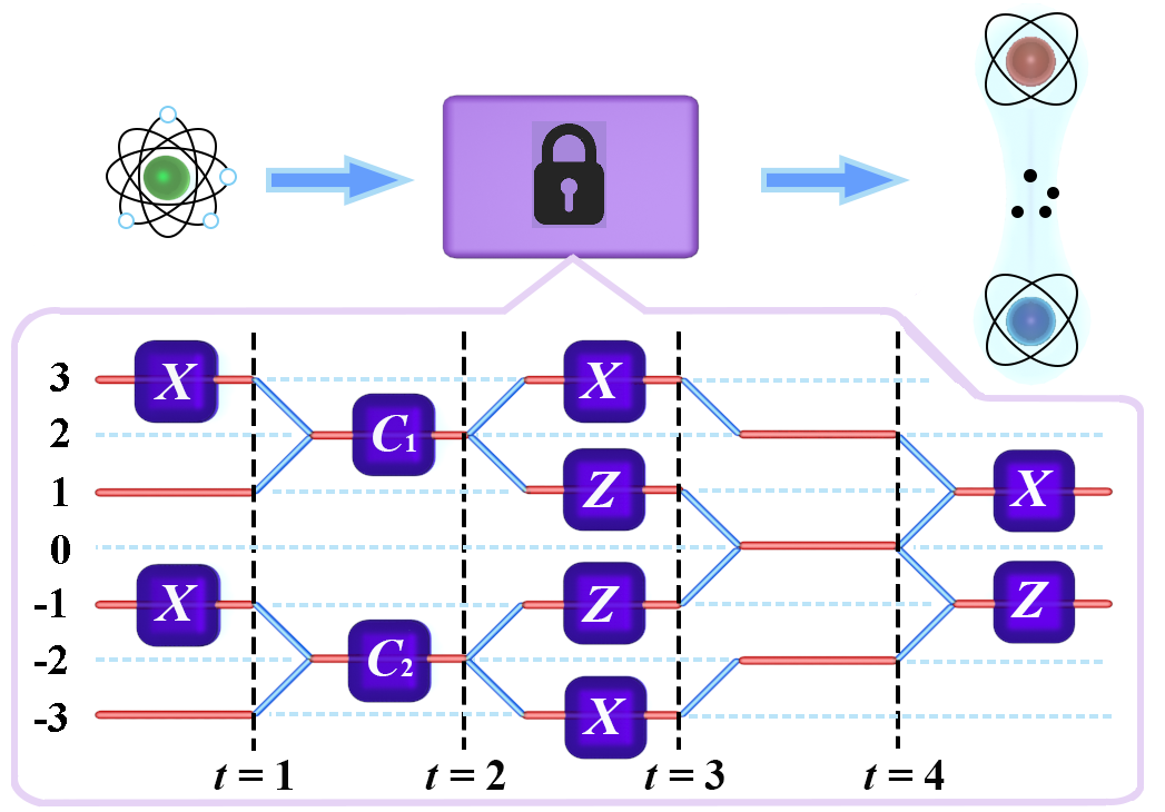
Figure 1: Schematic diagram of quantum information masking (upper plot) and realization of the masker $M$ of the real ququart based on a quantum walk (lower plot). The coin operators featuring in the figure are given by $X=\left(\begin{smallmatrix}0&1\\ 1&0\end{smallmatrix}\right)$, $Z=\left(\begin{smallmatrix}1&0\\ 0&-1\end{smallmatrix}\right)$, ${C}_{1}=\frac{1}{\sqrt{2}}\left(\begin{smallmatrix}\mathrm{i}&1\\ -\mathrm{i}&1\end{smallmatrix}\right)$, and ${C}_{2}=\frac{1}{\sqrt{2}}\left(\begin{smallmatrix}1&\mathrm{i}\\ -1&\mathrm{i}\end{smallmatrix}\right)$.

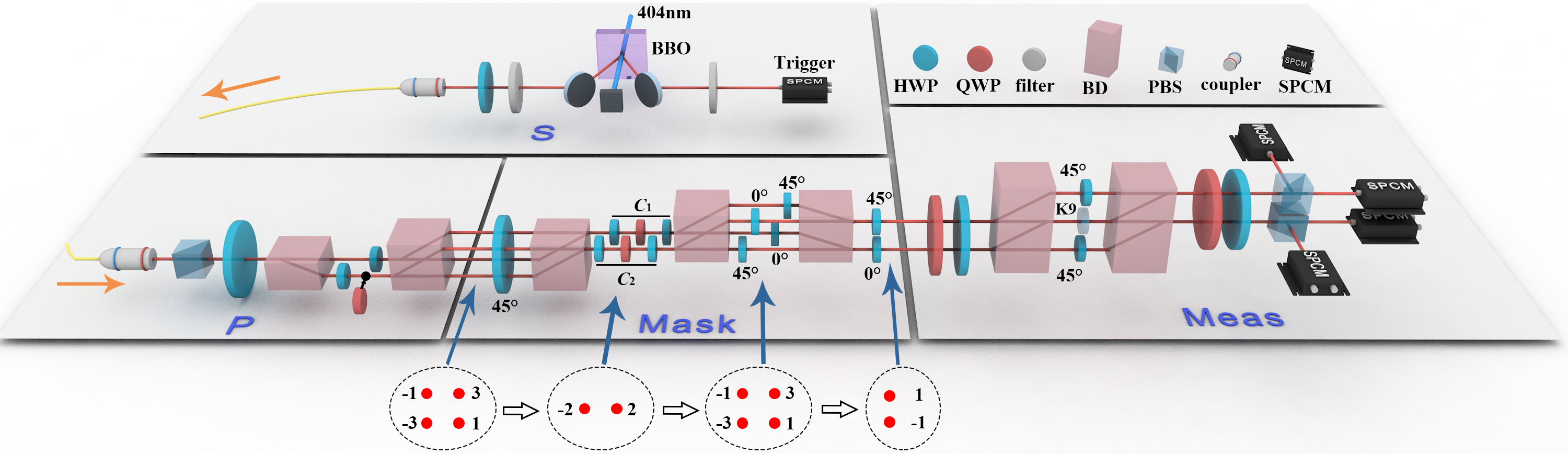
Figure 2: Experimental setup. The heralded single-photon source (labeled by S) on top is realized by spontaneous parametric down-conversion in a type-I $\beta$-barium-borate (BBO) crystal. The rest setup consists of three modules: state-preparation module (labeled by P), masking module (labeled by Mask), and measurement module (labeled by Meas). The masking module implements the masker defined in Eq. (3) according to the quantum-walk scheme illustrated in Fig. 1. The photon’s spatial modes labeled at the bottom correspond to the walker’s positions defined in Fig. 1. Two combinations of wave plates of the form HWP-QWP-HWP in the masking module realize the coin operators $C_{1}$ and $C_{2}$ defined in the caption of Fig. 1. HWP: half-wave plate; QWP: quarter-wave plate; BD: beam-displacer; PBS: polarizing beam-splitter; SPCM: single-photon counting module; K9: K9 glass plate.

To realize the masker $M$ of the real ququart, here we design a simple scheme based on a quantum walk as illustrated in Fig. 1, which can be implemented in a photonic system. In a quantum walk [36, 37, 38, 39], the state $|x,c\rangle$ of the walker-coin joint system is characterized by two indices $x$ and $c$, where $x=\dots,-1,0,1,\dots$ denotes the position of the walker on a one-dimensional chain, and $c=0,1$ labels the state of the coin qubit, which determines the moving direction of the walker in the next step. Each step of the quantum walk can be described by a unitary operator of the form $U(t)=\mathcal{T}C(t)$, where $C(t)=\sum_{x}|x\rangle\langle x|\otimes C(x,t)$, with $C(x,t)$ being position-dependent coin operators, and $\mathcal{T}$ is the conditional translation operator,

$$\mathcal{T}=\sum_{x}{(|x-1\rangle\langle x|\otimes|0\rangle\langle 0|+|x+1\rangle\langle x|\otimes|1\rangle\langle 1|)}.$$ (5)

The ququart can be encoded into the initial state (with $t$ = 0) of the walker-coin system using the path degree of freedom (DoF). To be concrete, a general pure state $|\psi\rangle=\sum_{j=0}^{3}{a_{j}|j\rangle}$ of the ququart with $\sum_{j=0}^{3}{|a_{j}|^{2}}=1$ is encoded as follows:

$$|\Psi\rangle=(a_{0}|-3\rangle+a_{1}|-1\rangle+a_{2}|1\rangle+a_{3}|3\rangle)\otimes|1\rangle.$$ (6)

After the first step of the quantum walk, the joint state evolves into

$$|\Psi_{1}\rangle=a_{0}|-2,1\rangle+a_{1}|-2,0\rangle+a_{2}|2,1\rangle+a_{3}|2,0\rangle.$$ (7)

After the second step, the joint state evolves into

$$|\Psi_{2}\rangle= \frac{\mathrm{i}a_{0}+a_{1}}{\sqrt{2}}|-3,0\rangle+\frac{\mathrm{i}a_{0}-a_{1}}{\sqrt{2}}|-1,1\rangle$$

$$+\frac{a_{2}+\mathrm{i}a_{3}}{\sqrt{2}}|1,0\rangle+\frac{a_{2}-\mathrm{i}a_{3}}{\sqrt{2}}|3,1\rangle.$$ (8)

Following a similar procedure, the final state after the quantum walk reads

$$|\Psi^{\prime}\rangle= \frac{a_{1}-\mathrm{i}a_{0}}{\sqrt{2}}|1,0\rangle-\frac{a_{1}+\mathrm{i}a_{0}}{\sqrt{2}}|-1,1\rangle$$

$$+\frac{a_{2}-\mathrm{i}a_{3}}{\sqrt{2}}|1,1\rangle+\frac{a_{2}+\mathrm{i}a_{3}}{\sqrt{2}}|-1,0\rangle$$

$$= -\mathrm{i}\bigl{(}a_{0}|\Phi_{0}^{\prime}\rangle+a_{1}|\Phi_{1}^{\prime}\rangle+a_{2}|\Phi_{2}^{\prime}\rangle+a_{3}|\Phi_{3}^{\prime}\rangle\bigr{)},$$ (9)

where

$$|\Phi_{0}^{\prime}\rangle =\frac{1}{\sqrt{2}}(|+1,0\rangle+|-1,1\rangle),$$ (10)

$$|\Phi_{1}^{\prime}\rangle =\frac{\mathrm{i}}{\sqrt{2}}(|+1,0\rangle-|-1,1\rangle),$$

$$|\Phi_{2}^{\prime}\rangle =\frac{\mathrm{i}}{\sqrt{2}}(|+1,1\rangle+|-1,0\rangle),$$

$$|\Phi_{3}^{\prime}\rangle =\frac{1}{\sqrt{2}}(|+1,1\rangle-|-1,0\rangle).$$

Now $|\Psi^{\prime}\rangle$ can be regarded as a two-qubit state on the Hilbert space $\mathcal{H}_{A}\otimes\mathcal{H}_{B}$, where $A$ denotes the effective walker qubit composed of positions $+1$ and $-1$, and $B$ denotes the coin qubit. Here $\{|\Phi_{j}^{\prime}\rangle\}_{j=0}^{3}$ is exactly the two-qubit magic basis in $\mathcal{H}_{A}\otimes\mathcal{H}_{B}$, so the quantum walk illustrated in Fig. 1 indeed realizes the masker $M$ defined in Eq. (3).

Experimental setup.—The setup for masking the real ququart is shown in Fig. 2. It contains four modules: a heralded single-photon source, a state-preparation module, a masking module, and a measurement module. Here we use the path DoF to encode the real ququart and the polarization DoF to encode the coin state employed in the quantum walk within the masking module.

In the module of single-photon source, an ultraviolet laser with central wavelength of 404nm is used to pump a type-I phase-matched beta-barium borate (BBO) crystal to generate a photon pair in a product (polarization) state via spontaneous parametric down-conversion [40]. One photon is measured as a trigger to herald the generation of its twin photon, which is then transmitted to the state-preparation module.

In the state-preparation module, a polarization beam splitter (PBS) first prepares the photon in the horizontal-polarization state $|H\rangle$ (in contrast with the vertical-polarization state $|V\rangle$). Then two beam displacers (BDs) and three half-wave plates (HWPs) transform the photon state into

$$(a_{0}|-3\rangle+a_{2}|1\rangle)\otimes|H\rangle+(a_{1}|-1\rangle+a_{3}|3\rangle)\otimes|V\rangle,$$ (11)

where the four real parameters $a_{i}$ for $i=0,...,3$ are controlled by three HWPs (see Appendix A). Finally, we prepare the ququart state

$$(a_{0}|-3\rangle+a_{1}|-1\rangle+a_{2}|1\rangle+a_{3}|3\rangle)\otimes|V\rangle$$ (12)

of the form in Eq. (6) by inserting a HWP at 45^∘ (which realizes the $X$ or NOT gate) on paths $-3$ and $1$ to turn $|H\rangle$ into $|V\rangle$. Note that the first two $X$ gates on paths $-1$ and $3$ in the masking module in Fig. 1 can also be implemented by a HWP at 45^∘; moreover, the four paths can share a same HWP placed at the beginning of the masking module in Fig. 2. The removable quarter-wave plate (QWP) in the preparation module is used only to prepare pure states with complex coefficients (see Appendix B).

After state preparation, the ququart is sent into the masking module, which realizes the quantum walk illustrated in Fig. 1. The two QWP-HWP-QWP combinations realize the coin operators $C_{1}$ and $C_{2}$, respectively, while the $0^{\circ}$ HWPs realize the $Z$ gates. The output of the masking module is a hybrid entangled state between the path qubit and the polarization qubit of the heralded photon.

The measurement module consists of two QWP-HWP combinations designed to control the measurement settings employed for measuring the path qubit and polarization qubit (see Appendix C). In addition, a K9 plate is used to compensate for different path lengths among the interference arms. Finally, the heralded photon is collected by four single-photon counting modules (SPCMs).

Experimental results.—To demonstrate the performance of the masking protocol realized using the photonic quantum walk as described above, we select the following four probe states:

$$\begin{gathered}|0\rangle,\quad\frac{1}{\sqrt{2}}(|0\rangle+|1\rangle),\\ \frac{1}{\sqrt{3}}(|0\rangle+|1\rangle+|2\rangle),\quad\frac{1}{2}(|0\rangle+|1\rangle+|2\rangle+|3\rangle),\end{gathered}$$ (13)

which form a complete but non-orthogonal basis in $\mathcal{H}$. To verify that the masking module indeed transforms these input states according to the theoretical prediction described in Eqs. (6)-(10), we perform fidelity estimation based on quantum state verification (QSV) [41, 42, 43] (see Appendix D) on the output states from the masking module. It turns out the fidelity between each output state and the ideal masked state is above 98%, as shown in Fig. 3. To further certify that no information of the input state can be inferred from each reduced state of the output state, we then perform quantum state tomography on the path and polarization qubits, respectively. In each case the average purity obtained in the experiment is very close to 0.5 as shown in Fig. 3, which implies that the reduced states of both subsystems are nearly completely mixed and little information about the original state can be retrieved from each subsystem alone; see Appendix E for more details. These experimental results clearly demonstrate that the masking module in Fig. 2 successfully realizes the masker $M$ in Eq. (3) within small experimental errors.

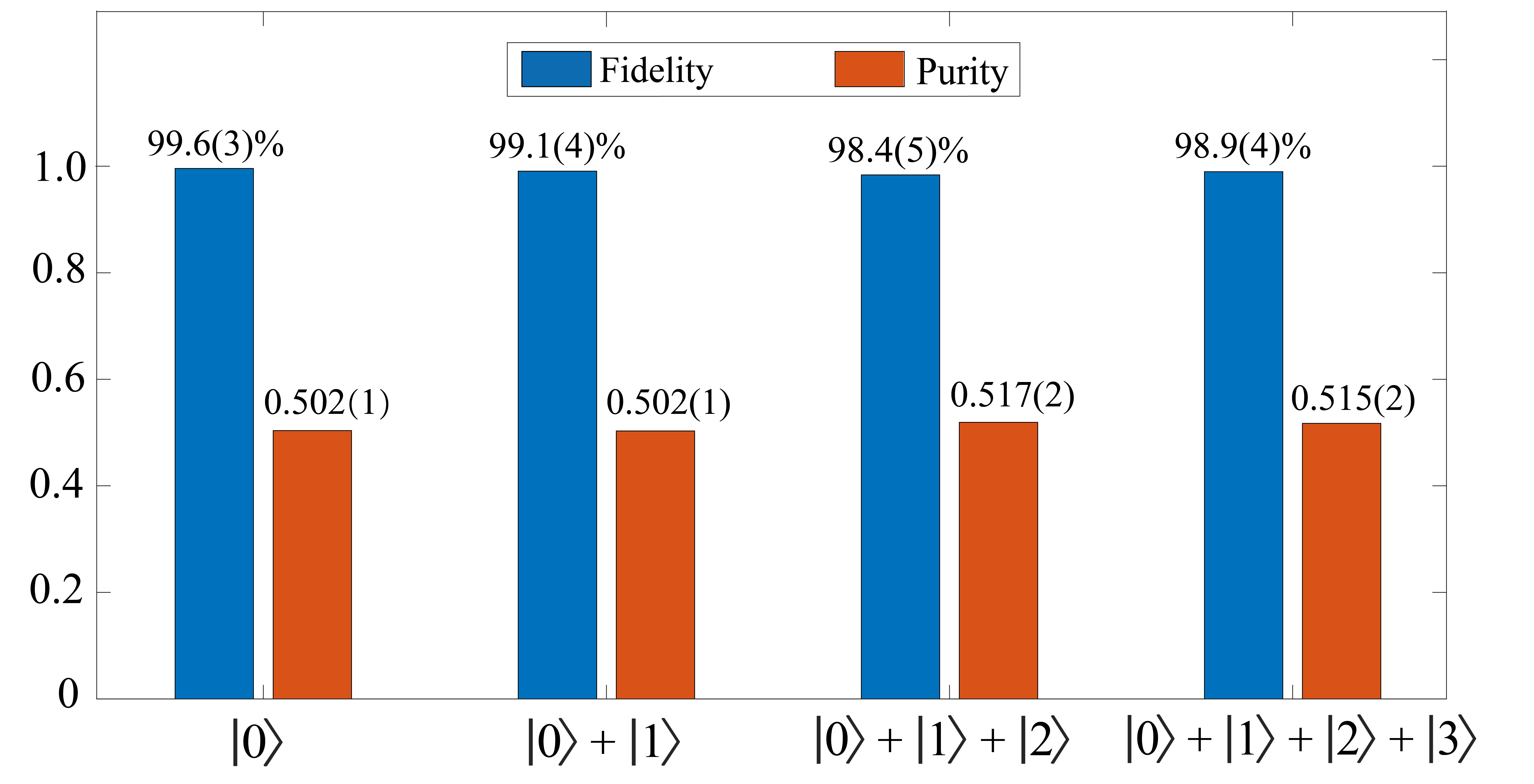
Figure 3: Experimental characterization of the masking module in Fig. 2. Each blue bar represents the fidelity between the actual output state and the ideal output state associated with each probe state as marked at the bottom of the figure. Each red bar represents the average purity of the two reduced states of the output state. The number in the parentheses above the blue (red) bar indicates the $95\%$ confidence interval of each fidelity estimator (the standard deviation of each purity estimator). The methods for quantifying the confidence interval and the standard deviation are detailed in Appendices D and E.

Next, we show that the information of the input state can be faithfully retrieved from the bipartite correlations of the output state of the masker $M$. To be concrete, the density matrix of any real state can be reconstructed from the correlation statistics of nine product Pauli measurements $\sigma_{j}\otimes\sigma_{k}$ for $j,k=x,y,z$ on the output state. In the experiment, each tensor product $\sigma_{j}\otimes\sigma_{k}$ is measured 4000 times to determine its mean value. The specific decoding method is detailed in Appendix F. As an example, the decoding result on the input state $(|0\rangle+|1\rangle+|2\rangle+|3\rangle)/2$ is shown in Fig. 4, and the decoding fidelity is 98.9%, which is consistent with the result of QSV shown in Fig. 3.

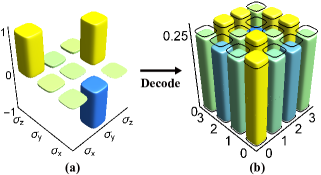
Figure 4: Experimental decoding of the masked state from correlation measurements. Here the input state is given by $(|0\rangle+|1\rangle+|2\rangle+|3\rangle)/2$. (a) Mean values $\langle\sigma_{i}\otimes\sigma_{j}\rangle$ for $i,j\in\{x,y,z\}$. (b) Matrix elements of the reconstructed density matrix (only real part is shown since the imaginary part is zero by reconstruction; see Appendix F). Bars without color represent the original input state, while bars with color represent the reconstructed state.

Figure 5: Relation between the concurrence of the output state and the robustness of imaginarity of the input state, which has the form $(|0\rangle+e^{i\phi}|1\rangle)/{\sqrt{2}}$ with $0\leq\phi\leq\pi/2$. The error bars represent the standard deviations of the concurrence estimations, which are determined via re-sampling (see Appendix E).

Finally, we verify the relation between the concurrence of the output state and the robustness of imaginarity of the input state as presented in Eq. (4). To be concrete, we choose input states of the form

$$|\psi(\phi)\rangle=\frac{1}{\sqrt{2}}(|0\rangle+e^{\mathrm{i}\phi}|1\rangle),\quad 0\leq\phi\leq\frac{\pi}{2}.$$ (14)

The robustness of imaginarity of the input state and the concurrence of the output state are respectively given by

$$\!\!\mathscr{I}_{R}(|\psi(\phi)\rangle)=\sin\phi,\quad C(M|\psi(\phi)\rangle)=\cos\phi.$$ (15)

In the experiment, the concurrence is determined by virtue of the formula $\mathcal{C}(|\Psi\rangle):=\sqrt{2(1-\operatorname{tr}(\varrho_{\mathrm{P}}^{2}))}$, where $\varrho_{\mathrm{P}}$ is the reduced state of the path qubit of the output state as determined by quantum state tomography (see Appendix E). The experimental results shown in Fig. 5 agree very well with the theoretical prediction, which implies that partial information of the input state is accessible to each subsystem once the robustness of imaginarity becomes nonzero. These results also corroborate the conclusion that $\mathcal{D}^{\mathrm{R}}(\mathcal{H})$ is a maximal maskable set.

Summary.—We experimentally realized a masking protocol of the real ququart using a photonic quantum walk. This is the first experiment on quantum information masking beyond a qubit system. Our experiment clearly demonstrates that quantum information of the real ququart can be completely hidden in bipartite correlations of hybrid entangled states, which is not accessible to each subsystem alone, but can be faithfully retrieved from correlation measurements. By contrast, any superset of the set of real density matrices cannot be masked. Furthermore, the entanglement of the output state is tied to the robustness of imaginarity of the input state. These results manifest a sharp distinction between real quantum mechanics and complex quantum mechanics in hiding and masking quantum information. Moreover, they offer valuable insights on the potential and limitation of quantum information masking, which are of intrinsic interest to many active research areas.

It should be pointed out that the two DoFs sharing the masked information in our experiment reside in the same location (photon), and the meaning of “masking” is slightly different from the common literature. Here the information is masked into the correlations between two DoFs instead of two space-separated particles. Nevertheless, the underlying mathematical structures in the two scenarios are identical. So the main conclusions obtained in our proof-of-principle experiment should apply to both scenarios. Also, in principle our experiment can be generalized to realize quantum information masking in two photons by cascading the protocol of quantum state fission [32] after the photonic quantum walk.

APPENDIX A: Preparation of pure states with real coefficients

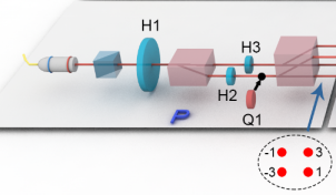
Figure A1: The preparation module of the experimental setup.

In this section we show that the state-preparation module in Fig. 2 in the main text (also shown in Fig. A1) can prepare an arbitrary pure state of the real ququart. Suppose the angles of the optical axes of H1, H2, and H3 in Fig. A1 are $h_{1}$, $h_{2}$, and $h_{3}$ (with respect to the horizontal direction), respectively. The input heralded photon is initially prepared in the state $|1\rangle\otimes|H\rangle$, which is turned into the following state

$$|1\rangle\otimes[\cos(2h_{1})|H\rangle+\sin(2h_{1})|V\rangle]$$ (A1)

by H1. The BD after H1 coherently routes the heralded photon to paths $-3$ and $1$ according to the polarization state of the heralded photon, which yields the state

$$|-3\rangle\otimes\cos(2h_{1})|H\rangle+|1\rangle\otimes\sin(2h_{1})|V\rangle.$$ (A2)

Then H2 and H3 transform the photon state into

$$|-3\rangle\otimes\bigl{[}\cos(2h_{1})\cos(2h_{2})|H\rangle+\cos(2h_{1})\sin(2h_{2})|V\rangle\bigr{]}$$

$$+|1\rangle\otimes\bigl{[}\sin(2h_{1})\sin(2h_{3})|H\rangle-\sin(2h_{1})\cos(2h_{3})|V\rangle\bigr{]}.$$ (A3)

Next, the second BD transforms the state of the heralded photon into

$$\bigl{[}\cos(2h_{1})\cos(2h_{2})|-3\rangle+\sin(2h_{1})\sin(2h_{3})|1\rangle\bigr{]}\otimes|H\rangle$$

$$+ \bigl{[}\cos(2h_{1})\sin(2h_{2})|-1\rangle-\sin(2h_{1})\cos(2h_{3})|3\rangle\bigr{]}\otimes|V\rangle.$$ (A4)

Finally, by inserting $45^{\circ}$ HWPs on paths $-3$ and $1$, we can prepare the following state,

$$\bigl{[} \cos(2h_{1})\cos(2h_{2})|-3\rangle+\cos(2h_{1})\sin(2h_{2})|-1\rangle$$ (A5)

$$+\sin(2h_{1})\sin(2h_{3})|1\rangle-\sin(2h_{1})\cos(2h_{3})|3\rangle\bigr{]}\otimes|V\rangle,$$

which has the form of Eq. (6) in the main text. Incidentally, this operation can also be performed in the masking module, as pointed out in the main text. To prepare the state in Eq. (6), we need to choose the parameters $h_{1}$, $h_{2}$, and $h_{3}$ so as to satisfy the following equations:

$$\cos(2h_{1})\cos(2h_{2}) =a_{0},$$ (A6)

$$\cos(2h_{1})\sin(2h_{2}) =a_{1},$$

$$\sin(2h_{1})\sin(2h_{3}) =a_{2},$$

$$-\sin(2h_{1})\cos(2h_{3}) =a_{3}.$$

APPENDIX B: Preparation of pure states with complex coefficients

In this section we show that the state-preparation module in Fig. 2 in the main text (also shown in Fig. A1) can also prepare certain pure states with complex coefficients as presented in Eq. (14) in the main text. By inserting Q1 into path $-3$ as marked in Fig. A1, we can prepare the states defined in Eq. (14). Such pure states with complex coefficients are required to demonstrate the relation between the concurrence of the output state and the robustness of imaginarity of the input state as presented in Eq. (4) in the main text.

To be specific, denote the angles of the optical axes of H1 and Q1 from the horizontal direction by $h_{1}$ and $q_{1}$. Now we set $q_{1}=45^{\circ}$ and $h_{1}=0^{\circ}$, then the state of the heralded photon after Q1 reads [44]

$$|-3\rangle\otimes\frac{1}{\sqrt{2}}\bigl{\{}[\cos(45^{\circ}-2h_{2})+\mathrm{i}\sin(45^{\circ}-2h_{2})]|H\rangle$$

$$+[\cos(45^{\circ}-2h_{2})-\mathrm{i}\sin(45^{\circ}-2h_{2})]|V\rangle\bigr{\}}.$$ (A7)

If we set $h_{2}=\frac{\phi}{4}+22.5^{\circ}$ (here $\phi$ is the parameter appearing in Eq. (14) in the main text), then the photon state after Q1 reduces to

$$|-3\rangle\otimes\frac{1}{\sqrt{2}}(|H\rangle+\mathrm{e}^{\mathrm{i}\phi}|V\rangle)$$ (A8)

up to a global phase. After the action of the second BD, the photon state becomes

$$\frac{1}{\sqrt{2}}(|-3\rangle|H\rangle+\mathrm{e}^{\mathrm{i}\phi}|-1\rangle|V\rangle).$$ (A9)

Finally, by inserting a 45^∘ HWP (which realizes the $X$ or NOT gate) on paths $-3$ and $1$, we can prepare the following state

$$\frac{1}{\sqrt{2}}(|-3\rangle+\mathrm{e}^{\mathrm{i}\phi}|-1\rangle)\otimes|V\rangle,$$ (A10)

which agrees with Eq. (14) in the main text. Note that this HWP can also be considered as a part of the masking module.

APPENDIX C: Implementation of local projective measurements

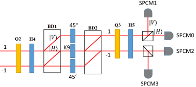
Figure A2: The measurement module of the experimental setup.

In this section, we show that the measurement module in Fig. 2 (also shown in Fig. A2) can perform an arbitrary local projective measurement on the path-polarization two-qubit system. Suppose we want to perform the projective measurement onto the product basis

$$\{|\varphi_{0}\rangle|\psi_{0}\rangle,|\varphi_{0}\rangle|\psi_{1}\rangle,|\varphi_{1}\rangle|\psi_{0}\rangle,|\varphi_{1}\rangle|\psi_{1}\rangle\},$$ (A11)

where

$$|\varphi_{0}\rangle =\cos\gamma|0\rangle+\mathrm{e}^{\mathrm{i}\zeta}\sin\gamma|1\rangle,$$ (A12)

$$|\varphi_{1}\rangle =\sin\gamma|0\rangle-\mathrm{e}^{\mathrm{i}\zeta}\cos\gamma|1\rangle,$$

$$|\psi_{0}\rangle =\cos\alpha|0\rangle+\mathrm{e}^{\mathrm{i}\beta}\sin\alpha|1\rangle,$$

$$|\psi_{1}\rangle =\sin\alpha|0\rangle-\mathrm{e}^{\mathrm{i}\beta}\cos\alpha|1\rangle.$$

To simplify the notation, here we temporarily use $|0\rangle$ ($|1\rangle$) to refer to “path 1” (“path $-1$”) for the path qubit, and to “horizontal polarization” (“vertical polarization”) for the polarization qubit. Then the output state from the masking module can be expressed as follows,

$$|\Psi\rangle=a_{0}|\varphi_{0}\rangle|\psi_{0}\rangle+a_{1}|\varphi_{0}\rangle|\psi_{1}\rangle+a_{2}|\varphi_{1}\rangle|\psi_{0}\rangle+a_{3}|\varphi_{1}\rangle|\psi_{1}\rangle.$$ (A13)

We first choose the angles of the optical axes of Q2 and H4 in Fig. A2 so as to implement the transformation $|\psi_{0}\rangle\to|0\rangle,\ |\psi_{1}\rangle\to|1\rangle$ on the polarization qubit (see Supplemental Material of Ref. [44] on how to calculate the angles), which turns $|\Psi\rangle$ into

$$|\Psi^{\prime}\rangle =(a_{0}|\varphi_{0}\rangle+a_{2}|\varphi_{1}\rangle)\otimes|0\rangle+(a_{1}|\varphi_{0}\rangle+a_{3}|\varphi_{1}\rangle)\otimes|1\rangle.$$ (A14)

Then the two BDs split and re-combine the two light beams, which turns $|\Psi^{\prime}\rangle$ into

$$|\Psi^{\prime\prime}\rangle=|0\rangle\otimes(a_{1}|\varphi_{0}\rangle+a_{3}|\varphi_{1}\rangle)+|1\rangle\otimes(a_{0}|\varphi_{0}\rangle+a_{2}|\varphi_{1}\rangle).$$ (A15)

Next, we set the angles of the optical axes of Q3 and H5 so as to realize the transformation $|\varphi_{0}\rangle\to|0\rangle,\ |\varphi_{1}\rangle\to|1\rangle$, which turns $|\Psi^{\prime\prime}\rangle$ into

$$|\Psi^{\prime\prime\prime}\rangle=a_{1}|0\rangle|0\rangle+a_{3}|0\rangle|1\rangle+a_{0}|1\rangle|0\rangle+a_{2}|1\rangle|1\rangle.$$ (A16)

Now, the probabilities that the heralded photon is found by SPCM 0, 1, 2, 3 are $|a_{1}|^{2}$, $|a_{3}|^{2}$, $|a_{0}|^{2}$, $|a_{2}|^{2}$, respectively. In this way, we can realize the local projective measurement onto the product basis in Eq. (A11).

APPENDIX D: Fidelity estimation based on quantum state verification

To estimate the fidelity between a two-qubit state $\varrho$ and the Bell state $|\Phi\rangle=(|00\rangle+|11\rangle)/\sqrt{2}$, we can apply the idea of quantum state verification according to Ref. [41]. To be specific, we can randomly perform one of the three local projective tests associated with the three test projectors $P_{XX}^{+}$, $P_{YY}^{-}$, $P_{ZZ}^{+}$, respectively, where

$$P_{XX}^{+}=\frac{\mathbbm{1}+X\otimes X}{2},$$ (A17)

$$P_{YY}^{-}=\frac{\mathbbm{1}-Y\otimes Y}{2},$$

$$P_{ZZ}^{+}=\frac{\mathbbm{1}+Z\otimes Z}{2},$$

and $\mathbbm{1}$ stands for the identity operator acting on the two-qubit system. To optimize the performance, each test is performed with probability $1/3$. The resulting verification operator reads

$$\Omega=\frac{1}{3}(P_{XX}^{+}+P_{YY}^{-}+P_{ZZ}^{+})=|\Phi\rangle\langle\Phi|+\frac{1}{3}(\mathbbm{1}-|\Phi\rangle\langle\Phi|).$$ (A18)

Now suppose that the fidelity between $\varrho$ and $|\Phi\rangle\langle\Phi|$ is $F(\varrho,|\Phi\rangle)=\langle\Phi|\varrho|\Phi\rangle=1-\epsilon$, where $\epsilon$ is the infidelity. Then the probability that $\varrho$ can pass each test on average is given by

$$p_{\mathrm{succ}}={\rm tr}(\varrho\Omega)=1-\frac{2}{3}\epsilon,$$ (A19)

which implies that

$$\epsilon=\frac{3}{2}(1-p_{\mathrm{succ}}).$$ (A20)

If $\varrho$ passes $S$ tests after $N$ tests in total in a given experiment, then $\hat{p}_{\mathrm{succ}}:=S/N$ is an unbiased estimator for $p_{\mathrm{succ}}$, from which we can construct an unbiased estimator for the infidelity,

$$\hat{\epsilon}=\frac{3}{2}(1-\hat{p}_{\mathrm{succ}}).$$ (A21)

To calculate the 95% confidence interval of $\hat{\epsilon}$, here we assume that all the states $\varrho$ in the $N$ runs are independent and identically distributed. A common choice for the 95% confidence interval of $\hat{p}_{\mathrm{succ}}$ is the Agresti-Coull interval [45], which has the form

$$\tilde{p}-\kappa_{\alpha}(\tilde{p}\tilde{q})^{1/2}\tilde{N}^{-1/2}\leq p_{\mathrm{succ}}\leq\tilde{p}+\kappa_{\alpha}(\tilde{p}\tilde{q})^{1/2}\tilde{N}^{-1/2},$$ (A22)

where

$$\tilde{p}=\frac{\tilde{S}}{\tilde{N}},\quad\tilde{q}=1-\tilde{p},\quad\tilde{S}=S+\frac{\kappa_{\alpha}^{2}}{2},\quad\tilde{N}=N+\kappa_{\alpha}^{2},$$ (A23)

and $\kappa_{\alpha}:=z_{\alpha/2}$ is the ($1-\alpha/2$)th quantile of the standard normal distribution. Accordingly, the 95% confidence interval of $\hat{\epsilon}$ reads

$$\epsilon_{\rm low}\leq\epsilon\leq\epsilon_{\rm high},$$ (A24)

where

$$\epsilon_{\rm low}=\frac{3}{2}\bigl{[}1-\tilde{p}-\kappa_{0.05}(\tilde{p}\tilde{q})^{1/2}\tilde{N}^{-1/2}\bigr{]},$$ (A25)

$$\epsilon_{\rm high}=\frac{3}{2}\bigl{[}1-\tilde{p}+\kappa_{0.05}(\tilde{p}\tilde{q})^{1/2}\tilde{N}^{-1/2}\bigr{]}.$$

When the target state changes from $|\Phi\rangle$ to, say, $|\Phi^{\prime}\rangle=(U\otimes\mathbbm{1}_{B})|\Phi\rangle$, the above approach still applies as long as the set of test projectors is replaced by $\{P_{X^{\prime}X}^{+},P_{-Y^{\prime}Y}^{+},P_{Z^{\prime}Z}^{+}\}$ accordingly, where $X^{\prime}=UXU^{\dagger}$, $Y^{\prime}=UYU^{\dagger}$, $Z^{\prime}=UZU^{\dagger}$.

In our experiment, the total number of tests is chosen to be $N=5000$ to reduce the statistical fluctuation. The values of $S$ associated with the four probe states indicated in Fig. 3 in the main text are $4986$, $4969$, $4946$, and $4963$, respectively. The estimation errors of the fidelities shown in Fig. 3 are determined by virtue of these numbers and the formula

$$\max\{\hat{\epsilon}-\epsilon_{\rm low},\epsilon_{\rm high}-\hat{\epsilon}\}.$$ (A26)

Note that the estimation error of each fidelity is the same as the estimation error of each infidelity.

APPENDIX E: Quantum state tomography of the path qubit and polarization qubit

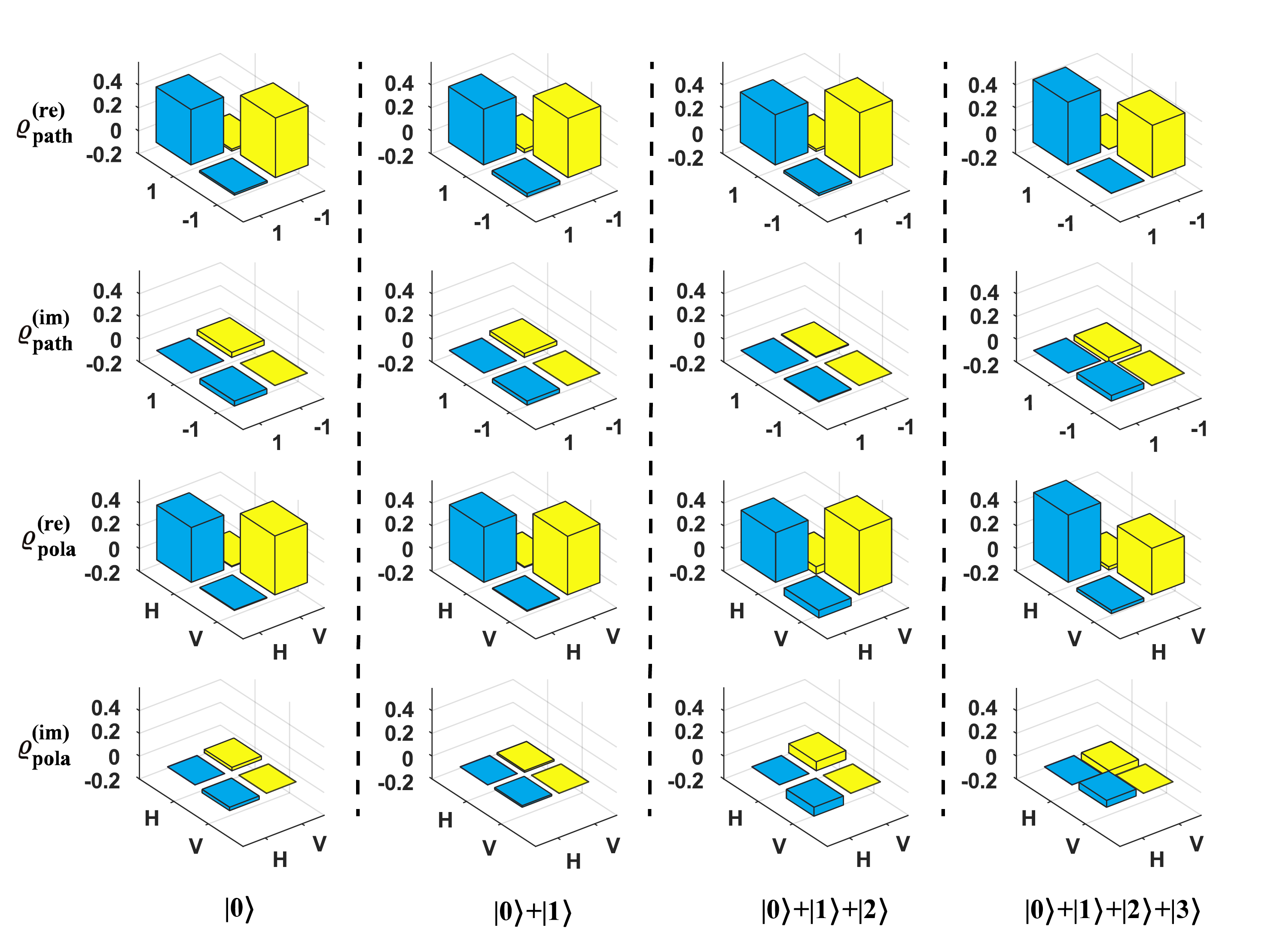
Figure A3: Experimental results on the reduced density matrices of the path qubit ($\varrho_{\rm path}$) and polarization qubit ($\varrho_{\rm pola}$), respectively, of the output states of the masker defined in Eq. (3) in the main text. Here “re” denotes the real part, and “im” denotes the imaginary part. The bottom line marks the input probe states associated with the output states. The experimental results demonstrate that all the reduced density matrices are nearly maximally mixed.

To further characterize the performance of the masking module, we perform quantum state tomography on the path qubit and polarization qubit of the output states associated with the four input states $|0\rangle$, $(|0\rangle+|1\rangle)/\sqrt{2}$, $(|0\rangle+|1\rangle+|2\rangle)/\sqrt{3}$, and $(|0\rangle+|1\rangle+|2\rangle+|3\rangle)/2$, respectively [cf. Eq. (13) in the main text]. To determine each reduced density matrix of each output state, $X$, $Y$, $Z$ measurements are performed 4000 times, respectively. Then the density matrix is reconstructed using the maximum-likelihood method described in Ref. [46]. The reconstruction results on the reduced density matrices are shown in Fig. A3.

By virtue of the above results we can compute the average purity of the two reduced density matrices of each output state, as shown in Fig. 3 in the main text. To determine the estimation error of the average purity, we re-sample $100$ times the photon-counting results used in the tomography according to the Poisson distribution, and then calculate the standard deviation of the average purity using the re-sampled data.

Since the output state is pure, its concurrence is determined by the purity of each reduced density matrix, which in turn can be determined by quantum state tomography. The concurrence shown in Fig. 5 in the main text is inferred from the purity of the density matrix of the path qubit using a similar way as mentioned above except that here $X$, $Y$, $Z$ measurements are performed 10000 times, respectively. To determine the estimation error of the concurrence, we re-sample $100$ times the photon-counting results used in the tomography of the path qubit according to the Poisson distribution, and then calculate the standard deviation of the concurrence using the re-sampled data.

APPENDIX F: Decoding input ququart from correlation measurements

In the main text, we introduced a simple masker $M:\mathcal{H}\mapsto\mathcal{H}_{A}\otimes\mathcal{H}_{B}$ for the real ququart associated with the Hilbert space $\mathcal{H}$, where both $\mathcal{H}_{A}$ and $\mathcal{H}_{B}$ are qubit Hilbert spaces. To be specific, $M$ is the isometry defined by its action on the computational basis:

$$M|j\rangle=-\mathrm{i}(U_{j}\otimes\mathbbm{1}_{B})|\Phi\rangle,\qquad j=0,1,2,3,$$ (A27)

where $U_{0}:=\mathbbm{1}_{A}$, $\{U_{j}\}_{j=1}^{3}:=\{\mathrm{i}\sigma_{z},\mathrm{i}\sigma_{x},\mathrm{i}\sigma_{y}\}$ forms a set of Hurwitz-Radon matrices on $\mathcal{H}_{A}$, and $|\Phi\rangle=(|00\rangle+|11\rangle)/\sqrt{2}$ is the canonical maximally entangled state in $\mathcal{H}_{A}\otimes\mathcal{H}_{B}$. Here we shall show that the information of the real input state can be faithfully decoded from the bipartite correlations of the output state of the masker $M$.

Recall that any two-qubit state $\varrho$ on $\mathcal{H}_{A}\otimes\mathcal{H}_{B}$ can be expressed as

$$\varrho=\frac{1}{4}\bigg{(}\mathbbm{1}+\bm{a}\cdot{\bm{\sigma}}\otimes\mathbbm{1}_{B}+\mathbbm{1}_{A}\otimes\bm{b}\cdot{\bm{\sigma}}+\sum_{j,k}{T_{jk}}\,\sigma_{j}\otimes\sigma_{k}\bigg{)},$$ (A28)

where $\bm{\sigma}=(\sigma_{x},\sigma_{y},\sigma_{z})$, $\bm{a}$ and $\bm{b}$ are the Bloch vectors of the two reduced states, respectively, and $T$ is the correlation matrix. The entries of the correlation matrix can be determined by suitable Pauli measurements according to the following equation

$$T_{jk}=\langle\sigma_{j}\otimes\sigma_{k}\rangle={\rm tr}[\varrho(\sigma_{j}\otimes\sigma_{k})],\quad j,k\in\{x,y,z\}.$$ (A29)

To decode the input state, we first consider the case in which the input real state is pure. A general real pure state in $\mathcal{H}$ can be written as $|\psi(\bm{c})\rangle=\sum_{j}c_{j}|j\rangle$, where $\bm{c}=(c_{0},c_{1},c_{2},c_{3})$ is a normalized real vector. The corresponding output state of the masker $M$ has the form

$$|\Psi(\bm{c})\rangle:=M|\psi(\bm{c})\rangle=-\mathrm{i}[U(\bm{c})\otimes\mathbbm{1}_{B}]|\Phi\rangle,$$ (A30)

where $U(\bm{c}):=\sum_{j=0}^{3}{c_{j}U_{j}}$. Note that

$$|\Phi\rangle\langle\Phi|=\frac{1}{4}(\mathbbm{1}+\sigma_{x}\otimes\sigma_{x}-\sigma_{y}\otimes\sigma_{y}+\sigma_{z}\otimes\sigma_{z}),$$ (A31)

and

$$U(\bm{c})\sigma_{x}U(\bm{c})^{\dagger} =(c_{0}^{2}-c_{1}^{2}+c_{2}^{2}-c_{3}^{2})\sigma_{x}+2(c_{2}c_{3}-c_{0}c_{1})\sigma_{y}+2(c_{0}c_{3}+c_{1}c_{2})\sigma_{z},$$ (A32)

$$U(\bm{c})\sigma_{y}U(\bm{c})^{\dagger} =2(c_{0}c_{1}+c_{2}c_{3})\sigma_{x}+(c_{0}^{2}-c_{1}^{2}-c_{2}^{2}+c_{3}^{2})\sigma_{y}+2(c_{1}c_{3}-c_{0}c_{2})\sigma_{z},$$

$$U(\bm{c})\sigma_{z}U(\bm{c})^{\dagger} =2(c_{1}c_{2}-c_{0}c_{3})\sigma_{x}+2(c_{1}c_{3}+c_{0}c_{2})\sigma_{y}+(c_{0}^{2}+c_{1}^{2}-c_{2}^{2}-c_{3}^{2})\sigma_{z}.$$

So the density operator of $|\Psi(\bm{c})\rangle$ reads

$$|\Psi(\bm{c})\rangle\langle\Psi(\bm{c})|=\frac{1}{4}\bigg{[}\mathbbm{1}+\sum_{j,k}{T(\bm{c})_{jk}}\,\sigma_{j}\otimes\sigma_{k}\bigg{]},$$ (A33)

where the correlation matrix $T(\bm{c})$ has the form

$$T(\bm{c})=\left(\begin{matrix}c_{0}^{2}-c_{1}^{2}+c_{2}^{2}-c_{3}^{2}&-2(c_{0}c_{1}+c_{2}c_{3})&2(c_{1}c_{2}-c_{0}c_{3})\\ 2(c_{2}c_{3}-c_{0}c_{1})&-(c_{0}^{2}-c_{1}^{2}-c_{2}^{2}+c_{3}^{2})&2(c_{1}c_{3}+c_{0}c_{2})\\ 2(c_{0}c_{3}+c_{1}c_{2})&-2(c_{1}c_{3}-c_{0}c_{2})&c_{0}^{2}+c_{1}^{2}-c_{2}^{2}-c_{3}^{2}\end{matrix}\right).$$ (A34)

In conjunction with the normalization condition $c_{0}^{2}+c_{1}^{2}+c_{2}^{2}+c_{3}^{2}=1$, we can deduce that

$$c_{0}^{2}=\frac{1}{4}(1+T_{11}-T_{22}+T_{33}),\qquad c_{1}^{2}=\frac{1}{4}(1-T_{11}+T_{22}+T_{33}),$$ (A35)

$$c_{2}^{2}=\frac{1}{4}(1+T_{11}+T_{22}-T_{33}),\qquad c_{3}^{2}=\frac{1}{4}(1-T_{11}-T_{22}-T_{33}),$$

and

$$c_{2}c_{3}=\frac{1}{4}(T_{21}-T_{12}),\qquad c_{1}c_{3}=\frac{1}{4}(T_{23}-T_{32}), c_{1}c_{2}=\frac{1}{4}(T_{13}+T_{31}),$$ (A36)

$$c_{0}c_{1}=-\frac{1}{4}(T_{21}+T_{12}),\qquad c_{0}c_{2}=\frac{1}{4}(T_{23}+T_{32}), c_{0}c_{3}=\frac{1}{4}(T_{31}-T_{13}).$$

By linearity the above result can be generalized to any mixed input state $\rho$ that has a real density matrix. In this case, in analogy to Eq. (A34), the correlation matrix of the output state $M\rho M^{\dagger}$ reads

$$T=\left(\begin{matrix}\rho_{00}-\rho_{11}+\rho_{22}-\rho_{33}&-2(\rho_{01}+\rho_{23})&2(\rho_{12}-\rho_{03})\\ 2(\rho_{23}-\rho_{01})&-(\rho_{00}-\rho_{11}-\rho_{22}+\rho_{33})&2(\rho_{13}+\rho_{02})\\ 2(\rho_{03}+\rho_{12})&-2(\rho_{13}-\rho_{02})&\rho_{00}+\rho_{11}-\rho_{22}-\rho_{33}\end{matrix}\right).$$ (A37)

Accordingly, we have

$$\rho_{00}=\frac{1}{4}(1+T_{11}-T_{22}+T_{33}),\qquad \rho_{11}=\frac{1}{4}(1-T_{11}+T_{22}+T_{33}),$$ (A38)

$$\rho_{22}=\frac{1}{4}(1+T_{11}+T_{22}-T_{33}),\qquad \rho_{33}=\frac{1}{4}(1-T_{11}-T_{22}-T_{33}),$$

and

$$\rho_{23}=\frac{1}{4}(T_{21}-T_{12}),\qquad \rho_{13}=\frac{1}{4}(T_{23}-T_{32}), \rho_{12}=\frac{1}{4}(T_{13}+T_{31}),$$ (A39)

$$\rho_{01}=-\frac{1}{4}(T_{21}+T_{12}),\qquad \rho_{02}=\frac{1}{4}(T_{23}+T_{32}), \rho_{03}=\frac{1}{4}(T_{31}-T_{13}),$$

which generalize Eqs. (A35) and Eq. (A36). Therefore, the density matrix of any real input state of the ququart can be faithfully decoded from the correlation matrix of the output state, which can easily be determined by virtue of product Pauli measurements $\sigma_{j}\otimes\sigma_{k}$ for $j,k\in\{x,y,z\}$.

References

Braunstein and Pati [2007]S. L. Braunstein and A. K. Pati, Quantum information cannot
be completely hidden in correlations: Implications for the black-hole
information paradox, Phys. Rev. Lett. 98, 080502 (2007).
Modi et al. [2018]K. Modi, A. K. Pati,
A. Sen(De), and U. Sen, Masking quantum information is impossible, Phys. Rev. Lett. 120, 230501 (2018).
Wootters and Zurek [1982]W. K. Wootters and W. H. Zurek, A single quantum cannot be
cloned, Nature 299, 802 (1982).
Lamas-Linares et al. [2002]A. Lamas-Linares, C. Simon, J. C. Howell, and D. Bouwmeester, Experimental quantum cloning of single
photons, Science 296, 712 (2002).
Barnum et al. [1996]H. Barnum, C. M. Caves,
C. A. Fuchs, R. Jozsa, and B. Schumacher, Noncommuting mixed states cannot be broadcast, Phys. Rev. Lett. 76, 2818 (1996).
Hillery et al. [1999]M. Hillery, V. Bužek, and A. Berthiaume, Quantum secret
sharing, Phys. Rev. A 59, 1829 (1999).
Hayden and Preskill [2007]P. Hayden and J. Preskill, Black holes as mirrors:
quantum information in random subsystems, J. High Energy Phys. 2007, 120 (2007).
Liu et al. [2018]Z.-W. Liu, S. Lloyd, E. Zhu, and H. Zhu, Entanglement, quantum randomness, and complexity beyond
scrambling, J. High Energy Phys. 2018, 41 (2018).
Li et al. [2019a]B. Li, S.-H. Jiang,
X.-B. Liang, X. Li-Jost, H. Fan, and S.-M. Fei, Deterministic versus probabilistic quantum information masking, Phys. Rev. A 99, 052343 (2019a).
Liang et al. [2020]X.-B. Liang, B. Li, S.-M. Fei, and H. Fan, Impossibility of masking a set of quantum states of nonzero
measure, Phys. Rev. A 101, 042321 (2020).
Du et al. [2020]Y. Du, Z. Guo, H. Cao, K. Han, and C. Yang, Masking quantum information encoded in pure and mixed states, Int. J. Theor. Phys. (2020).
Zhu [2020]H. Zhu, Hiding and masking quantum
information in complex and real quantum mechanics (2020), arXiv:2010.07843
[quant-ph] .
Li and Wang [2018]M.-S. Li and Y.-L. Wang, Masking quantum information in
multipartite scenario, Phys. Rev. A 98, 062306 (2018).
Wu et al. [2021]K.-D. Wu, T. V. Kondra,
S. Rana, C. M. Scandolo, G.-Y. Xiang, C.-F. Li, G.-C. Guo, and A. Streltsov, Operational resource theory of imaginarity, Phys. Rev. Lett. 126, 090401 (2021).
Wootters [1986]W. K. Wootters, Quantum mechanics
without probability amplitudes, Found. Phys. 16, 391 (1986).
Chiribella et al. [2011]G. Chiribella, G. M. D’Ariano, and P. Perinotti, Informational
derivation of quantum theory, Phys. Rev. A 84, 012311 (2011).
Ghosh et al. [2020]T. Ghosh, S. Sarkar,
B. K. Behera, and P. K. Panigrahi, Masking of quantum information into
restricted set of states (2020), arXiv:1910.00938 [quant-ph] .
Liu et al. [2021]Z.-H. Liu, X.-B. Liang,
K. Sun, Q. Li, Y. Meng, M. Yang, B. Li, J.-L. Chen, J.-S. Xu, C.-F. Li, and G.-C. Guo, Photonic
implementation of quantum information masking, Phys. Rev. Lett. 126, 170505 (2021).
Samal et al. [2011]J. R. Samal, A. K. Pati, and A. Kumar, Experimental test of the quantum no-hiding
theorem, Phys. Rev. Lett. 106, 080401 (2011).
Kalra et al. [2019]A. R. Kalra, N. Gupta,
B. K. Behera, S. Prakash, and P. K. Panigrahi, Demonstration of the no-hiding theorem on the 5-Qubit
IBM quantum computer in a category-theoretic framework, Quantum Inf. Process. 18, 170 (2019).
Englert et al. [2001]B.-G. Englert, C. Kurtsiefer, and H. Weinfurter, Universal unitary gate
for single-photon two-qubit states, Phys. Rev. A 63, 032303 (2001).
Fiorentino and Wong [2004]M. Fiorentino and F. N. C. Wong, Deterministic controlled-not
gate for single-photon two-qubit quantum logic, Phys. Rev. Lett. 93, 070502 (2004).
Vitelli et al. [2013]C. Vitelli, N. Spagnolo,
L. Aparo, F. Sciarrino, E. Santamato, and L. Marrucci, Joining the quantum state of two photons into one, Nat. Photonics 7, 521 (2013).
Hurwitz [1922]A. Hurwitz, Über die
Komposition der quadratischen Formen, Math. Ann. 88, 1 (1922).
HR [2006]Hurwitz-Radon matrices revisited: From effective solution
of the Hurwitz matrix equations to Bott periodicity, in Mathematical Survey Lectures 1943–2004 (Springer, Berlin, Heidelberg, 2006) pp. 141–153.
Hou et al. [2018]Z. Hou, J.-F. Tang,
J. Shang, H. Zhu, J. Li, Y. Yuan, K.-D. Wu, G.-Y. Xiang, C.-F. Li, and G.-C. Guo, Deterministic realization of collective
measurements via photonic quantum walks, Nat. Commun. 9, 1414 (2018).
Tang et al. [2020]J.-F. Tang, Z. Hou, J. Shang, H. Zhu, G.-Y. Xiang, C.-F. Li, and G.-C. Guo, Experimental
optimal orienteering via parallel and antiparallel spins, Phys. Rev. Lett. 124, 060502 (2020).
Li et al. [2019b]Z. Li, H. Zhang, and H. Zhu, Implementation of generalized measurements on a
qudit via quantum walks, Phys. Rev. A 99, 062342 (2019b).
Kwiat et al. [1999]P. G. Kwiat, E. Waks,
A. G. White, I. Appelbaum, and P. H. Eberhard, Ultrabright source of polarization-entangled
photons, Phys. Rev. A 60, R773(R) (1999).
Pallister et al. [2018]S. Pallister, N. Linden, and A. Montanaro, Optimal verification of entangled
states with local measurements, Phys. Rev. Lett. 120, 170502 (2018).
Zhu and Hayashi [2019a]H. Zhu and M. Hayashi, Efficient verification of pure quantum
states in the adversarial scenario, Phys. Rev. Lett. 123, 260504 (2019a).
Zhu and Hayashi [2019b]H. Zhu and M. Hayashi, General framework for verifying pure
quantum states in the adversarial scenario, Phys. Rev. A 100, 062335 (2019b).
Hou et al. [2016]Z. Hou, H. Zhu, G.-Y. Xiang, C.-F. Li, and G.-C. Guo, Error-compensation measurements on polarization qubits, J. Opt. Soc. Am. B 33, 1256 (2016).
Brown et al. [2001]L. D. Brown, T. T. Cai, and A. DasGupta, Interval estimation for a binomial
proportion, Statist. Sci. 16, 101 (2001).
Ježek et al. [2003]M. Ježek, J. Fiurášek, and Z. Hradil, Quantum inference of states and processes, Phys. Rev. A 68, 012305 (2003).