AAA-least squares rational approximation and solution of Laplace problems

Abstract

A two-step method for solving planar Laplace problems via rational approximation is introduced. First complex rational approximations to the boundary data are determined by AAA approximation, either globally or locally near each corner or other singularity. The poles of these approximations outside the problem domain are then collected and used for a global least-squares fit to the solution. Typical problems are solved in a second of laptop time to 8-digit accuracy, all the way up to the corners, and the conjugate harmonic function is also provided. The AAA-least squares combination also offers a new method for avoiding spurious poles in other rational approximation problems, and for greatly speeding them up in cases with many singularities. As a special case, AAA-LS approximation leads to a powerful method for computing the Hilbert transform or Dirichlet-to-Neumann map.

Mathematics Subject Classification 2020. Primary 41A20; Secondary 30E10, 44A15, 65N35

Keywords. rational approximation, AAA algorithm, lightning Laplace solver, conformal mapping, Hilbert transform, Dirichlet-to-Neumann map

1 Introduction

The aim of this paper is to introduce a new method for the numerical solution of planar Laplace problems, based on a combination of local complex rational approximations by the AAA algorithm followed by a real linear least-squares problem. This method is an outgrowth of three previous works [8, 15, 23], which we now briefly summarize.

The AAA algorithm (adaptive Antoulas–Anderson, pronounced “triple-A”) is a fast and flexible method for near-best complex rational approximation [23]. Given a vector $Z$ of real or complex sample points and a corresponding vector $F$ of data values, it finds a rational function $r$ of specified degree or accuracy such that

$$r(Z)\approx F.$$ (1.1)

This is done by developing a barycentric representation for $r$ by alternating a nonlinear step of greedy selection of the next barycentric support point with a linear least-squares approximation step to determine barycentric weights. If $F$ is obtained by a sampling a function $f(z)$ with singularities at certain points of $Z$, such as logarithms and fractional powers, then root-exponential convergence with respect to the degree $n$ is typically achieved (i.e., errors $O(\exp(-C\sqrt{n}\kern 1.0pt))$ for some $C>0$), with poles of the approximants $f$ clustering exponentially near the singularities [32]. The standard implementation of AAA approximation is the code aaa in Chebfun [10].

The lightning Laplace solver is a method for solving Laplace problems

$$\Delta u=0\hbox{ on $\Omega$},\quad u=h(z)\hbox{ on $\partial\Omega$}$$ (1.2)

on a simply connected domain $\Omega$ in the plane, which we parametrize for convenience by the complex variable $z$ [15]. It also computes an analytic function $f(z)$ such that $u=\hbox{\rm Re\kern 0.8pt}f$. This method first fixes poles with exponential clustering near each corner of $\Omega$ or other point where a singularity is expected. A real linear least-squares problem is then solved to determine a rational function in $\Omega$ with the prescribed poles, plus a polynomial term (i.e., poles at infinity), whose real part matches the boundary data as closely as possible. The method converges root-exponentially with respect to the number of poles and generalizes to Neumann boundary data, multiply connected domains, and the Stokes and Helmholtz equations [7, 14]. The standard implementation is the MATLAB code laplace available at [30].

Although the lightning Laplace solver is fast and effective, one would really like to solve Laplace problems by a method more like the AAA algorithm, which allows the set $Z$ to be completely arbitrary and adapts to the singularities of the solution automatically rather than relying on a priori estimates of pole clustering. Two challenges have held back the development of a AAA method for Laplace problems. First, no barycentric representation is known for real parts of rational functions. Second, even if such a formula were available, there would remain the fundamental problem of achieving approximation in a region $\Omega$ based on values on the boundary $\partial\Omega$. A AAA-style approximation does not distinguish interior from exterior and includes no mechanism to restrict poles to the latter.

These considerations led to the third contribution that this work builds upon, published on arXiv by the first author in 2020 [8]. The upper row of Figure 1 illustrates the idea as applied to the “NA Digest model problem” [29], an L-shaped region with boundary data $u(z)=(\hbox{\rm Re\kern 0.8pt}z)^{2}$. First, complex AAA is used to approximate the real data on the boundary. The resulting analytic function is complex (though real on $\partial\Omega$, up to the approximation accuracy), with poles both inside and outside $\Omega$. Then the poles in $\Omega$ are discarded, leaving a set of poles outside $\Omega$ that are often clustered effectively for rational approximation. The Laplace problem is solved by computing such an approximation by linear least-squares fitting on $\partial\Omega$.

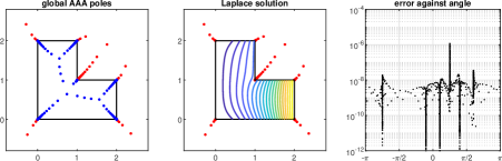
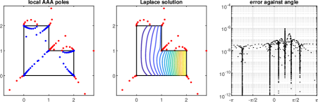
Figure 1: Above, Costa’s AAA-Laplace method from [8]. A global AAA approximation gives poles both inside and outside $\Omega$. The poles inside are discarded, and those outside are used for a linear least-squares fit. Errors on the boundary in the rightmost plot are plotted against angle with respect to the point $(1+i\kern 0.7pt)/2$. This computation determines $u(0.99+0.99i)\approx 1.0267919261073$ to 10 digits of accuracy, but it takes 12 secs. of laptop time because the AAA approximation has $294$ poles. Below, the new local variant, in which the poles outside $\Omega$ are determined by local AAA approximations near each corner. The computation time falls to $0.67$ secs. because the AAA problems are six times smaller, without much change in accuracy.

In the form just described, the AAA-Laplace method can be quite slow because of depending on AAA approximations with a large number of poles. In this article we propose a variation that often speeds it up greatly, namely, to use local AAA approximations near each singularity to choose the set of poles. Since the cost of AAA approximation grows with the fourth power of the number of poles, this leads to a speedup potentially by a factor on the order of the cube of the number of corners. For the L-shaped example the speedup is a factor of about $18$.

The AAA-Laplace method as presented in [8] was actually much slower than indicated in Figure 1 for an accidental reason. In that implementation, aaa was invoked in its default “cleanup” mode, which led to the removal of many poles close to the singularities and a consequent need to compute AAA approximations involving as many as $1000$ poles. What that paper interpreted as a halving of the number of digits of accuracy due to discarding poles in $\Omega$ now seems to have been a consequence of using the cleanup feature. Throughout this paper, we always call aaa with “cleanup off”.

2 Laplace problems

Our main interest is problems with corner singularities, since this is where the power and convenience of rational functions are most decisive. However, the AAA approach can be effective for smooth problems too. Figure 2 presents an example. An irregular domain $\Omega$ (bounded by a trigonometric interpolant through 15 complex data points) is given with the Laplace boundary condition $u(z)=-\log|z|$. The vector $Z$ is constructed by sampling $\partial\Omega$ in $1000$ points, and a global AAA fit to the boundary data with tolerance $10^{-8}$ yields $46$ poles in $\Omega$ and $30$ in ${\mathbb{C}}\backslash\overline{\Omega}$. The interior poles are discarded, and a least-squares fit to the boundary data is computed via a $1000\times 102$ matrix: 60 real degrees of freedom for 30 poles and 42 for a polynomial term of degree $20$. The computation takes $0.7$ secs., and the maximum error on $Z$ is $2.1\times 10^{-9}$. A polynomial expansion needs about 10 times as many degrees of freedom to achieve the same accuracy, a ratio that would worsen exponentially for more distorted regions according to the theory of the “crowding phenomenon” in complex analysis [16, Thm. 5].

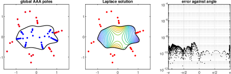
Figure 2: A smooth Laplace problem solved by the global AAA-LS method. A global AAA approximation produces 46 poles inside $\Omega$ and 30 outside, and the latter are retained for a real least-squares problem that also includes a polynomial term. 9-digit accuracy is achieved in $0.7$ secs.

We now turn to problems with singularities, typically at corners, whose locations are assumed to be known in advance. The local variant of the AAA-LS algorithm proceeds in this manner:

1. Construct sample point vector $Z$ and fix corresponding data values $H=h(Z)$.

2. For each singularity, run AAA for nearby sample points and data values.

3. Discard poles in $\overline{\Omega}$ and retain poles exterior to $\overline{\Omega}\kern 0.5pt$.

4. Calculate real least-squares fit to boundary data, including a polynomial term.

5. Construct function handles for $u(z)$ and its analytic extension $f(z)$.

We give some mathematical and MATLAB details of each of these steps. The global variant of the algorithm is the same except that step 2 involves just a single global AAA approximant.

1. Construct sample point vector $Z$ and fix corresponding data values $H=h(Z)$. The problem domain $\Omega$ can be quite arbitrary, and it can be multiply connected. Typically $Z$ will consist of hundreds or thousands of points, which it is simplest to specify in advance with exponential clustering near singularities. In MATLAB we use constructions like logspace(-14,0,300)’ for a singularity at one endpoint of $[\kern 0.5pt0,1]$ and tanh(linspace(-16,16,600)’) for singularities at both endpoints of $[-1,1]$. If AAA-LS software were to be developed analogous to the laplace code of [30] for the lightning Laplace method, then it would be worthwhile placing sample points more strategically to avoid having too many more rows in the matrix than necessary.

2. For each singularity, run AAA for nearby sample points and data values. We use the simplest choice: each point of $Z$ is associated with whichever singularity it is closest to (on the same boundary component, if the geometry is multiply connected so there are several boundary components). The Chebfun command aaa is invoked with ’cleanup’,’off’, and throughout this paper we specify a AAA tolerance of $10^{-8}$.

3. Discard poles in $\overline{\Omega}$ and retain poles exterior to $\overline{\Omega}\kern 0.5pt$. The aaa code returns highly accurate pole locations computed via a matrix generalized eigenvalue problem described in [23]. To distinguish those inside and outside $\Omega$, we use the complex variant inpolygonc = @(z,w) inpolygon(real(z),imag(z),real(w),imag(w)) of the inpolygon command.

4. Calculate real least-squares fit to boundary data, including a polynomial term. If pol is a row vector of the poles from step 3 and n is a small nonnegative integer, the sequence

    d = min(abs(Z-pol),[],1);
    P = Z.^(0:n); Q = d./(Z-pol);
    A = [real(P) real(Q) -imag(P) -imag(Q)];
    c = reshape(A\H,[],2)*[1;1i];

computes a complex coefficient vector $c$ for the function $f$ in the space spanned by the polynomials of degree $n$ and the given poles such that $u=\hbox{\rm Re\kern 0.8pt}f$ is the least-squares fit to the data $H$ in the sample points. The vector $d$ contains the distances of the poles to $Z$ and is used to scale the columns of $Q$ to have $\infty$-norm 1.  For $n$ much larger than 10, however, numerical stability requires that the monomials of Z.^(0:n) be replaced by orthogonalizations computed by the Vandermonde with Arnoldi procedure of [6]. This can be done by replacing P = Z.^(0:n) by [Hes,P] = VAorthog(Z,n), where the code VAorthog comes from [7] and is listed in the appendix.

The description and code above apply for bounded, simply connected domains with Dirichlet boundary conditions. For problems with Neumann boundary conditions on some sides, the corresponding rows of $A$ are modified appropriately. For exterior domains, $z$ is replaced by $(z-z_{c})^{-1}$ for some point $z_{c}$ in the hole. For multiply-connected domains, additional columns of the form $\log|z-z_{j}|$ must be added where $\{z_{j}\}$ are a set of a fixed points, one in each hole [2, 28]. In addition, new columns are added corresponding to polynomials in $1/(z-z_{j})$ for each $j$.

5. Construct function handles for $u(z)$ and its analytic extension $f(z)$. For convenience in making plots and other applications, it is desirable to have functions that can be applied to matrices as well as vectors. Following the commands above this can be achieved with

    f = @(z) reshape([z(:).^(0:n) d./(z(:)-pol)]*c,size(z));
    u = @(z) real(f(z)); v = @(z) imag(f(z));

When VAorthog is used, the first line is replaced by

    f = @(z) reshape([VAeval(z(:),Hes) d./(z(:)-pol)]*c,size(z));

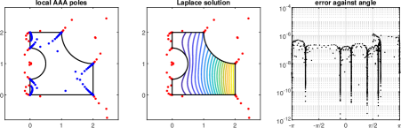
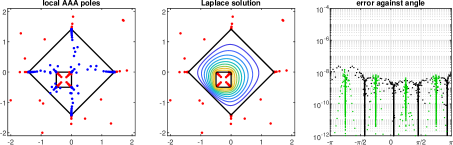
Figure 3: Two examples of Laplace solutions by the local AAA-LS method. Above, a square with two circular bites removed. The computation involves 102 poles outside the domain and a polynomial of degree $20$. Below, a multiply connected domain, solved in 1.7 secs. with 397 poles outside the domain and a polynomial of degree 40. In the error plot, black dots correspond to the outer boundary and green dots to the inner one. The boundary data used for local-AAA pole location are not those of the Laplace problem, as explained in the text.

Figure 3 illustrates the method at work on two examples. In the first row, the L shape of Figure 1 has been modified to a square with two circular bites removed. No new issues arise here, as the method does not distinguish between straight and curved sides, so long as they are smooth. The second row shows a doubly-connected problem, and here some new issues do arise. First there is the use of polynomials with respect to both $z$ and $(z-z_{c})^{-1}$ as described above (writing $z_{c}$ instead of $z_{1}$ since there is just one hole), as well as the introduction of a $\log|z-z_{c}|$ term; we take $z_{c}=-(1+i\kern 0.5pt)/4$. The domain is discretized by 400 clustered points on each of the eight side segments, and the polynomials in $z$ and $(z-z_{c})^{-1}$ are of degree 40. A more fundamental issue also arises in this problem. The boundary data have been taken as $1$ on the inner square and $0$ on the outer square, a natural situation for a heat flow or electrostatics problem in a doubly connected geometry. Since these boundary conditions are constant on each of the two boundary components, however, the local AAA problems will be trivial and no poles at all will be produced! Clearly that is no route to an accurate solution, so for this computation, poles have been generated by using an artificial boundary condition (the square root of the product of the distances to the eight corners) and then the least-squares problem is solved with the boundary data actually prescribed. The reader is justified if he/she finds this puzzling, and we discuss the matter further in Section 6.

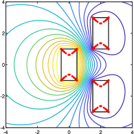
Figure 4: Local AAA-LS solution of a Laplace problem in an unbounded triply-connected domain, requiring reciprocal polynomials with respect to three interior points $c_{j}$ and also logarithm terms $\log|z-z_{j}|$. The computation takes 2 secs. and gives the value $u(1)\approx 0.64357510429036$ to 10-digit accuracy.

Our final example of this section is an unbounded region with three rectangular holes, shown in Figure 4. The boundary conditions are $u=1$ on the rectangle at the left and $u=0$ on the other two, giving a natural interpretation as the potential around three conductors. Each boundary segment is discretized by 400 clustered points, so the least-squares matrix has 4800 rows. The AAA fits lead to 52 poles inside a rectangle near each corner, 624 in total, and we also have a reciprocal-polynomial of degree 10 and one real logarithm term in each rectangle, bringing the number of columns of the matrix to $2\times(624+3\times 11)+3=1317$. A solution is computed in 2 secs. to 10-digit accuracy as measured by the value at the point $z=1$ midway between the rectangles, $u(1)\approx 0.64357510429036$.

A fine point to note in this triply-connected example is that the point $z=\infty$ is a point of analyticity, in the interior of the domain, so there should be no logarithmic term there, meaning that the sum of the coefficients of the three log terms centered at the points $z_{1},z_{2},z_{3}$ in the rectangles should be zero. This condition can be enforced by adding one more row to the matrix, or (as was in fact done for the computation in the figure) by taking the log columns of the matrix to correspond not to $\log|z-z_{j}|$ but to $\log|z-z_{j}|-\log|z-z_{j(\hbox{\scriptsize mod }3)+1}|$.

3 Conformal mapping

A Laplace solver that also produces the harmonic conjugate of the solution, hence its analytic extension, can be used to compute conformal maps. Details are given in [31], so here we give just one example of construction of the conformal map $g$ of a simply-connected region $\Omega$ containing the point $z=0$ to the unit disk, with $g(0)=0$ and $g^{\prime}(0)>0$. The trick is to write $g$ in the form

$$g(z)=z\exp(f(z)),\quad f(z)=\log(g(z)/z),$$ (3.1)

where $f$ is the unique nonzero analytic function on $\Omega$ has real part $-\log|z|$ on $\partial\Omega$ and imaginary part $0$ at $z=0$. Thus $f$ is obtained by solving a Laplace Dirichlet problem, and (3.1) then gives the map $g$.

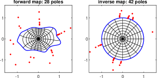
Figure 5: Conformal map of the region of Figure 2 by the global AAA-LS method. The map is computed to 8-digit accuracy in $0.8$ secs. and the rational approximations in both directions are evaluable in less than 1 $\mu$sec per point. In the left image, the poles differ slightly from those of Figure 2 because a further AAA compression of $z\exp(f(z))$ has taken place.

Figure 5 illustrates this method for the smooth region of Figure 2, where $-\log|z|$ was already the boundary condition. Thus the conformal map comes from exponentiating the analytic extension of the harmonic function of Figure 2 and multiplying the result by $z$. As described in [16], this result is then compressed by AAA approximation, and another AAA approximation gives the inverse map. See [31] for extensions to multiply connected regions.

The speed of these computations is remarkable. After an initial 0.9 secs. to construct the forward and inverse maps in this example, they can be each then be evaluated in 0.3 $\mu$secs. per point. For example, we take one million random points uniformly distributed in the unit disk, map them conformally to $\Omega$, then map these images back to the unit disk again. The whole back-and-forth process takes $0.6$ secs., and the maximum error in the million sample points is $1.1\times 10^{-8}$.

4 Rational approximation without spurious poles

Though the emphasis in this paper is on Laplace problems, AAA-LS approximation also offers striking advantages for more general rational approximations. It may be much faster than AAA alone for problems with a number of singularities, and since unwanted poles can be discarded, it produces approximations guaranteed to have desired properties of analyticity and stability. Thus AAA-LS may combat what Heather Wilber has called the “spurious poles blues” (discussed in [34], though without this phrase).

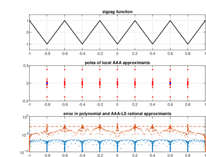
Figure 6: Top, a real zigzag function on $[-1,1]$ to be approximated over the whole interval by a single rational function. Middle, the 466 poles determined by local AAA fits near each singularity, each of degree 51 or 52. Two poles lie in $[-1,1]$ and are discarded (blue). Bottom, the resulting errors in the AAA-LS fit show accuracy of $3\times 10^{-7}$. A polynomial with the same 962 degrees of freedom such as a Chebyshev interpolant (dots) could have accuracy at best $10^{-3}$ (dashed line).

We illustrate both the speed and the robustness with an example of approximating a real zigzag function on the interval $[-1,1]$, shown in Figure 6.  Knowing that poles will need to cluster exponentially at the points $-0.8,-0.6,\dots,0.8$, we set up a 3000-point grid consisting of -0.9 + 0.2*tanh(linspace(-16,16,300)) and its nine translates at centers $-0.7,-0.5,\dots,0.9$.  With straight AAA approximation, poles in $[-1,1]$ virtually always appear. They could be removed for input to a least-squares fit, but the timing would still be very slow for the moderately large degrees needed for effective approximation: $0.3$, $4.2$, and $35.3$ seconds on our laptop for degrees $50$, $200$, and $500$.  By contrast, with its local AAA fits the AAA-LS method quickly computes a good approximation. In the figure, AAA-LS has been run with AAA tolerance $10^{-8}$, leading to local fits each of size $51$ and $52$ and hence quite speedy. This gives $466$ poles all together, two of which lie in $[-1,1]$ and are discarded, as shown in the middle panel of the figure. A least-squares fit with these 464 poles, plus a polynomial of degree 16, then gives the error marked in blue in the bottom figure, with maximum error $3.1\times 10^{-7}$. The whole computation takes half a second, and the resulting approximation can be evaluated in 5 $\mu$secs. per point. By contrast a polynomial fit with the same 962 degrees of freedom can have error no smaller than $1.6\times 10^{-3}$, as marked by the red dashed line. The red dots show the error for a polynomial Chebyshev interpolant of that degree.

It appears that AAA-LS offers a flexible, fast, and reliable way to compute near-best rational approximations with no unwanted poles. Potential applications lie in many areas of computational science and engineering. An interesting question is, might AAA-LS be further leveraged via a AAA-Lawson iteration as in [24] to lead to truly minimax rational approximations in certain cases?  For this to be possible, it would be necessary first to convert the rational approximation to barycentric form. We have not explored this possibility.

5 Computing the Hilbert transform

If $u$ is a sufficiently smooth real function defined on the real line, its Hilbert transform is the function $v$ defined by the principal value integral

$$v(y)={1\over\pi}\hbox{\kern 2.0ptPV\kern-2.0pt}\int_{-\infty}^{\infty}{u(x)\over y-x}\kern 0.8ptdx.$$ (5.1)

The transform can be interpreted as follows: if $f$ is a complex analytic function in the upper half-plane with $\hbox{\rm Re\kern 0.8pt}f(x)=u(x)$ for $x\in{\mathbb{R}}$, then $v(y)=\hbox{\rm Im\kern 0.8pt}f(y)$. Similar definitions and interpretations apply to the unit circle and other contours. Another name for the Hilbert transform (essentially) is the Dirichlet-to-Neumann map.

It is evident that to compute the Hilbert transform numerically, it suffices to find an analytic function in the upper half-plane whose real part on ${\mathbb{R}}$ matches that of $u$ to sufficient accuracy. The classical idea of this kind is to use a Fourier transform, perhaps discretized on a finite interval by the Fast Fourier Transform [20, p. 203]. For example, this is the method used by the hilbert command in the MATLAB Signal Processing Toolbox. But it is also possible to use rational approximations instead of trigonometric polynomials, and numerical methods of this kind have been proposed [22, 27, 33].

The AAA-LS method provides another natural approach based on rational approximation, since poles in the upper half-plane can be discarded to ensure the appropriate analyticity. Indeed, all of our AAA-LS Laplace solutions can be regarded as Hilbert transforms, but on more general contours $\partial\Omega$. A prototype code for the real line can be written like this:

   function [v,f] = ht(u)
   X = logspace(-10,10,300)’; X = [X; -X];       % sampling grid
   [~,pol] = aaa(u(X),X,’cleanup’,0);            % global AAA fit
   pol(imag(pol)>=0) = []; pol = pol.’;          % discard unwanted poles
   d = min(abs(X-pol),[],1);                     % for column normalization
   A = d./(X-pol); A = [real(A) -imag(A)];       % fitting matrix
   c = reshape(A\u(X),[],2)*[1;1i];              % least-squares solve
   f = @(x) reshape((d./(x(:)-pol))*c,size(x));  % analytic extension
   v = @(x) imag(f(x));                          % Hilbert transform

This is not an item of software—it is a proof of concept. Note that the sampling grid has been taken as 300 points exponentially spaced from $10^{-10}$ to $10^{10}$ and their negatives, 600 points all together. This would not be appropriate for all functions, but it is a good starting point for a function which loses analyticity possibly at $0$ and at $\infty$. The code does well at computing Hilbert transforms of the seven example functions Weideman lists in Table 1 of his paper [33]. In 0.6 secs. total on a laptop it produces results for these seven example problems with relative accuracy in the range of 5–13 digits, as detailed in Table 1. We shall not attempt systematic comparisons with other algorithms, but as an indication of the nontriviality of these computations, we mention that applying the MATLAB hilbert command for $u(x)=\exp(-x^{2})$ on a grid of 1024 equispaced points in $[-20,20\kern 0.5pt]$ gives an estimate of $v(2)$ with an error of $1.4\times 10^{-2}$, 11 orders of magnitude greater than the figure in Table 1.

Table 1: The example functions $u(x)$ from Table 1 by Weideman [33] together with their Hilbert transforms $v(x)$ evaluated at the arbitrary point $x=2$. In a total time of $0.6$ secs., the prototype AAA-LS code ht computes these numbers to 5–13 digits of relative accuracy.

Function $u$	Hilbert transform $v(2)$	AAA-LS error
$1/(1+x^{2})$	$0.400000000000000$	$-1.3\hbox{\kern 1.0pte}{-}12$
$1/(1+x^{4})$	$0.415945165403851$	$-4.3\hbox{\kern 1.0pte}{-}14$
$\sin(x)/(1+x^{2})$	$0.156805255543717$	$\hphantom{-}3.4\hbox{\kern 1.0pte}{-}06$
$\sin(x)/(1+x^{4})$	$0.121897775700258$	$-1.7\hbox{\kern 1.0pte}{-}07$
$\exp(-x^{2})$	$0.340026217066066$	$\hphantom{-}1.0\hbox{\kern 1.0pte}{-}13$
$\hbox{sech}(x)$	$0.506584586167368$	$\hphantom{-}1.3\hbox{\kern 1.0pte}{-}10$
$\exp(-|x|)$	$0.328435745958114$	$-1.4\hbox{\kern 1.0pte}{-}12$

Figure 7 illustrates AAA-LS computation of the Hilbert transform graphically for Weideman’s final example,

$$u(x)=e^{-|x|},\quad v(y)=\pi^{-1}\hbox{sign}(y)\bigl{[}e^{|y|}E_{1}(|y|)+e^{-|y|}Ei(|y|)\bigr{]},$$ (5.2)

where $E_{1}$ and $Ei$ are the exponential integrals computed in MATLAB by expint and ei. For each of the values $L=1,2,\dots,6$, a sample grid of $60L$ points $y$ has been used consisting of $30L$ points exponentially spaced from $10^{-L}$ to $10^{\kern 1.0ptL}$ and their negatives. Rapid convergence is observed to an accuracy of better than $10$ digits, despite the singularity of $u$ at $x=0$.

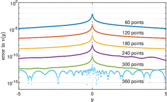
Figure 7: Error at $1000$ points $y\in[-5,5]$ in the Hilbert transform of $u(x)=\exp(-|x|)$ computed by the global AAA-LS method from $60,120,\dots,360$ exponentially spaced samples. This plot was produced in 2 secs. on a laptop.

The great flexibility of the AAA-LS method for computing the Hilbert transform is to be noted. It can work with arbitrary data points, which need not be regularly spaced, and it delivers a result as a global representation speedily evaluated via a function handle. No interpolation of data is required (see discussion of this problem in [9]), and singularities in $u(x)$ cause little degradation of accuracy so long as there are sample points clustered nearby, as illustrated in the example of Figure 7.

Many generalizations of this AAA-LS Hilbert transform computation are possible, including other contours both open and closed and more general Riemann–Hilbert problems.

6 Theoretical observations

The core of the AAA-LS method (in its global form) is the following idea, which we shall call the pole symmetry principle. Suppose $r$ is a complex rational approximation that closely approximates a real function $h$ on the boundary $\partial\Omega$ of a region $\Omega$. Then there is another complex rational function $r_{+}$, with poles only at the locations of the poles of $r$ outside $\Omega$, such that $\hbox{\rm Re\kern 0.8pt}r_{+}$ also closely approximates $h$ on $\partial\Omega$. The AAA-LS method finds $r$ by AAA approximation on $\partial\Omega$, extracts its poles outside $\Omega$, and then finds $r_{+}$ by linear least-squares fitting on $\partial\Omega$.

In particular, for cases with singularities on $\partial\Omega$, rational functions $r$ exist with root-exponential convergence to $h$ as $n\to\infty$ [15]. Such approximations will usually have poles that cluster exponentially on both sides of $\partial\Omega$ near each singularity. The pole symmetry principle proposes that we can discard all the poles inside $\Omega$, retaining only the ones outside $\Omega$, and still get essentially the same root-exponential convergence.

In this section we assess this idea. Our conclusions can be summarized as follows:

1. If $\Omega$ is a half-plane or a disk, the pole symmetry principle holds exactly (Theorems 6.1 and 6.2).

2. If $\Omega$ is a simply-connected domain with corners, the pole symmetry principle fails in the worse case in that $r_{+}$ may have no poles near $\partial\Omega$ even though they are needed to resolve singularities; conversely it may have clusters of poles near $\partial\Omega$ when they are not needed (examples shown in Figure 8).  However, both of these situations are nongeneric. For most problems, the principle holds also on regions with corners.

3. If $\Omega$ is a simply-connected domain bounded by an analytic curve, then in a certain theoretical sense it can be reduced to the case of a disk. However, the constants involved may be sufficiently adverse that in practice, it may be more appropriate to think of $\Omega$ as a domain with corners. Again the pole symmetry principle will usually hold even if this cannot be guaranteed in the worst case.

4. If $\Omega$ is a multiply-connected domain, then harmonic functions in $\Omega$ can in general not be approximated by rational functions: logarithmic terms are needed too. Thus the pole symmetry principle is inapplicable and a local rather than global variant of AAA-LS should be used.

To establish conclusion (1), let ${{\mathbb{C}}_{-}}$ and ${{\mathbb{C}}_{+}}$ denote the open lower and upper complex half-planes, respectively, and let $\|\cdot\|_{E}$ denote the supremum norm over a set $E$. The two assertions of the following theorem ensure that complex rational approximation on ${\mathbb{R}}$ produces “enough poles” to solve the Laplace problem on ${{\mathbb{C}}_{+}}$, and that it does not produce “too many poles” to be efficient.

Theorem 6.1.

Given a bounded real continuous function $h$ on ${\mathbb{R}}$, let $u$ be the bounded harmonic function in ${{\mathbb{C}}_{+}}$ with $u(x)=h(x)$ for $x\in{\mathbb{R}}$. Suppose there exists a rational function $r$, also real on ${\mathbb{R}}$, such that $\|r-h\|_{\mathbb{R}}\leq\varepsilon$ for some $\varepsilon\geq 0$. Then there exists a rational function $r_{+}$ whose poles are precisely the poles of $r$ in ${{\mathbb{C}}_{-}}$ such that $\|\hbox{\rm Re\kern 0.8pt}r_{+}-h\|_{\mathbb{R}}\leq\varepsilon$ and thus by the maximum principle also $\|\hbox{\rm Re\kern 0.8pt}r_{+}-u\|_{{\mathbb{C}}_{+}}\leq\varepsilon$. Conversely, if $r_{+}$ is a rational function analytic in ${{\mathbb{C}}_{+}}$ such that $\|\hbox{\rm Re\kern 0.8pt}r_{+}-u\|_{{\mathbb{C}}_{+}}\leq\varepsilon$, then there exists a rational function $r$ whose poles are the poles of $r_{+}$ and their reflections in ${{\mathbb{C}}_{+}}$ such that $\|r-h\|_{\mathbb{R}}\leq\varepsilon$.

Proof.

Given $r$ as indicated in the first assertion, write $r(z)=(r_{+}(z)+r_{-}(z))/2$, where $r_{+}$ has its poles in ${{\mathbb{C}}_{-}}$ and $r_{-}$ has its poles in ${{\mathbb{C}}_{+}}$. By the Schwarz reflection principle, $r(\overline{z})=\overline{r(z)}$ for all $z\in{\mathbb{C}}$, and thus the poles of $r_{-}$ must be the conjugates of the poles of $r_{+}$. Symmetry further implies

$$r_{-}(z)=\overline{r_{+}(\overline{z})}~{}~{}\forall z\in{\mathbb{C}},~{}\quad r(x)=\hbox{\rm Re\kern 0.8pt}r_{+}(x)~{}~{}\forall x\in{\mathbb{R}},$$ (6.1)

assuming that the constant $r(\infty)$, if it is nonzero, is split equally between $r_{-}$ and $r_{+}$. Thus $\hbox{\rm Re\kern 0.8pt}r_{+}(z)$ is a bounded harmonic function in ${{\mathbb{C}}_{+}}$ with $\|\hbox{\rm Re\kern 0.8pt}r_{+}-h\|_{\mathbb{R}}\leq\varepsilon$, hence also $\|\hbox{\rm Re\kern 0.8pt}r_{+}-u\|_{{\mathbb{C}}_{+}}\leq\varepsilon$ by the maximum principle. Moreover, the poles of $r_{+}$ are exactly the poles of $r$ in ${{\mathbb{C}}_{-}}$. Conversely, given $r_{+}$ as indicated in the second assertion, the function $r(z)=(r_{+}(z)+\overline{r_{+}(\overline{z})})/2$ has the required properties. ∎

The other half of conclusion (1) concerns the case of the open unit disk ${\Delta}$. Let $S$ denote the unit circle and ${\Delta_{-}}$ the complement of $\overline{{\Delta}}$ in ${\mathbb{C}}\cup\{\infty\}$. We get essentially the same theorem as before.

Theorem 6.2.

Given a real continuous function $h$ on $S$, let $u$ be the harmonic function in ${\Delta}$ with $u(x)=h(x)$ for $x\in S$. Suppose there exists a rational function $r$, also real on $S$, such that $\|r-h\|_{S}\leq\varepsilon$ for some $\varepsilon\geq 0$. Then there exists a rational function $r_{+}$ whose poles are precisely the poles of $r$ in ${\Delta_{-}}$ such that $\|\hbox{\rm Re\kern 0.8pt}r_{+}-h\|_{S}\leq\varepsilon$ and thus also $\|\hbox{\rm Re\kern 0.8pt}r_{+}-u\|_{\Delta}\leq\varepsilon$. Conversely, if $r_{+}$ is a rational function analytic in ${\Delta}$ such that $\|\hbox{\rm Re\kern 0.8pt}r_{+}-u\|_{\Delta}\leq\varepsilon$, then there exists a rational function $r$ whose poles are the poles of $r_{+}$ and their reflections in ${\Delta}$ such that $\|r-h\|_{S}\leq\varepsilon$.

Proof.

One can argue as before, or alternatively, derive this is a corollary of Theorem 6.1 by a Möbius transformation. ∎

We now turn to conclusion (2), concerning the case where $\Omega$ has corners. As mentioned, in the worst case rational approximation may give “too many poles,” meaning poles not needed for approximation of the solution of the Laplace problem, and it may give “not enough poles,” meaning poles that are inadequate to approximate the solution of the Laplace problem. To explain this, we present a pair of examples in Figure 8, both showing poles of AAA approximations with tolerance $10^{-8}$ on the boundary of the bounded symmetric “lens” domain $\Omega$ bounded by two circular arcs meeting at right angles at $z=\pm 1$.

The first image illustrates “too many poles.” When the function $h(z)=\hbox{\rm Re\kern 0.8pt}z$ is approximated by a rational function on $\partial\Omega$, many poles appear both inside and outside $\Omega$; this will be the rule almost always when a region has corners. And yet this boundary data can be exactly matched by the harmonic function $u(z)=\hbox{\rm Re\kern 0.8pt}z$, which has just a single pole at $\infty$. So the clusters of poles obtained by AAA are unnecessary for the Laplace problem in the interior of $\Omega$.

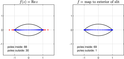
Figure 8: Examples showing that in the worst case, the pole symmetry principle underlying the global AAA-LS method may fail. On the left, AAA approximation gives “too many poles,” with poles exponentially clustered outside $\Omega$ near $\pm 1$ even though the singularity-free function $u(z)=\hbox{\rm Re\kern 0.8pt}z$ solves the Laplace problem. On the right, it gives “too few poles,” providing no poles at all outside $\Omega$ near the boundary even though the rational approximation of the solution of the Laplace problem will need them to approximate the branch point singularities at $\pm 1$. Both these situations are nongeneric and unlikely to appear in practice.

The second image illustrates “too few poles.” Here $h$ is taken as the values on $\partial\Omega$ of the analytic function $f$ that maps the exterior of $\Omega$ conformally to the exterior of the slit $[-1,1]$ while leaving the points $\pm 1$ and $\infty$ fixed:

$$f(z)={1+v^{2}\over 1-v^{2}},\quad v=-\left({z-1\over z+1}\right)^{2/3}.$$ (6.2)

With the standard branch of the $2/3$ power, $f$ has a branch cut along $[-1,1]$, and AAA finds a rational approximation $r$ whose poles lie approximately on this slit. In particular, they all lie within $\Omega$ apart from one pole of magnitude $10^{10}$, approximating the pair $f(\infty)=\infty$. Thus there are no poles near $\partial\Omega$ for the AAA-LS method to work with in approximating the solution in the interior of $\Omega$, yet this solution has singularities at $\pm 1$ involving fractional powers $(z\pm 1)^{4/3}$, so it would need such poles to get high accuracy.

Thus we see that on domains with corners, failure of the pole symmetry principle is possible. However, the failures we have identified are atypical, at least in these extreme forms. The example on the left in Figure 8 is special in that despite the corners in the domain, the solution to the Laplace problem has no singularities thanks to special boundary data. This is hardly the generic situation (though picking such examples is a common mistake beginners make when testing their Laplace codes!). As for the example on the right, it has the unusual property of involving data $h$ that can be analytically continued to all of ${\mathbb{C}}\cup\{\infty\}\backslash\overline{\Omega}$. This is another very special situation. Generically, a function $h$ on a domain boundary with corners will only be analytically continuable with branch cuts on both sides, and rational approximations will need to have poles approximating those branch cuts on both sides of the domain. Configurations like that of the second image of Figure 8 are unlikely to appear in applications.

Now we turn to conclusion (3). Suppose $\Omega$ is a simply-connected domain bounded by an analytic curve that is not simply a circle or straight line. For such a problem, Schwarz reflection no longer gives a symmetry equivalence between $\Omega$ and ${\mathbb{C}}\cup\{\infty\}\backslash\overline{\Omega}$. What happens to the pole symmetry principle?

The “pure mathematics answer” is that everything works essentially as before, modified only by the need for a fast exponentially-convergent polynomial term to be added into the rational approximations. The reasoning here can be based on the technique of considering a conformal map $w=\phi(z)$ of ${\mathbb{C}}\cup\{\infty\}\backslash\overline{\Omega}$ to ${\mathbb{C}}\cup\{\infty\}\backslash\overline{\Delta}$ with $\phi(\infty)=\infty$ and its inverse map $z=\psi(w)$ [12]. If $\partial\Omega$ is analytic, then $\phi$ and $\psi$ extend analytically to larger domains, implying that they can be approximated by polynomials in $z^{-1}$ and $w^{-1}$, respectively, with exponential convergence. It follows that rational approximation of a function $h$ defined on $\partial\Omega$, for example, is equivalent to rational approximation of its transplant $\tilde{h}(w)=h(\psi(w))$ on $S$, up to exponentially convergent polynomial terms. If $h$ has singularities, then root-exponential convergence of rational approximations in $z$ is ensured by the same property for rational approximation of $\tilde{h}$ in $w$. By this kind of reasoning one can argue that AAA-LS in a smooth domain is like AAA-LS in a disk, up to constants associated with polynomial approximations.

The “applied mathematics answer” is not so simple. All across complex analysis, the constants that appear in estimates of interest tend to grow exponentially as functions of geometric parameters such as the aspect ratios of reentrant or salient fingers in boundary curves, and this applies here. So the practical status of the pole symmetry principle for regions with curved boundaries may not be so different from that for regions with corners.

All the discussion above pertains to the global variant of AAA-LS.  For local variants, as illustrated in the discussion around the multiply-connected domain of Figure 3, failures of the algorithm are more likely to appear in practice if the AAA step of the algorithm is applied with the data $h$ given. In such cases, we recommend the method used in that figure: replace the actual boundary data $h$ by a function $\hat{h}$ targeted to generate singularities at each corner, such as the product of the square roots of the distances to the corners. Our experience shows that as a practical matter, this strategy is highly effective. The reason for this is that, though not all singularities look alike, a wide range of them can be approximated with root-exponential convergence by exponentially clustered poles, whose configurations need not be tuned to the singularities [15, 32]. So the set of poles utilized by AAA to approximate one function will generally also do well for another.

In the case of a multiply connected domain, to turn to point (4) of our summary, one should always use a local variant of the AAA-LS method. The reason is that approximating harmonic functions in such a domain will require logarithmic terms since their conjugates are in general multi-valued [2]. One can use AAA to approximate a real function $h$ on the boundary $\partial\Omega$ of such a domain by a rational function $r$, but $r$ will not have the right properties interior to $\Omega$. As illustrated in Figure 9, typically it will approximate different analytic functions near the different boundary components, separated by strings of poles approximating branch cuts (compare Fig. 6.9 of [23]). These poles have nothing to do with the harmonic function $u$ in $\Omega$ one wants to approximate, so in such a case global rational approximations should not be used.

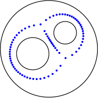
Figure 9: Poles of a global AAA rational approximant $r$ with tolerance $10^{-8}$ on the boundary of a triply-connected domain with boundary data $0$, $1$, and $2$ on the smaller, larger, and outer circles, respectively. The function $r$ matches the data accurately on all three parts of $\partial\Omega$, but achieves this only by introducing strings of poles that effectively split $\Omega$ into subdomains with separate analytic functions. Here, these are the constant functions $0$, $1$, and $2$, though the configuration would be much the same for any analytic boundary data. Effective approximation by a single harmonic function throughout $\Omega$ would require an additional logarithmic term in each hole, so for Laplace problems in domains like this, a local rather than global variant of AAA-LS should be used.

In discussing local rational approximations above, we alluded to a kind of approximate university of pole distributions for resolving singularities. This suggests that in the end, AAA approximation should not really be necessary; one could equally well use a “lightning” strategy in which poles are positioned a priori rather than determined from the data. Indeed we think this is likely to be the case for problems dominated by singular corners, though the great convenience of starting from AAA approximations remains an advantage. For problems less controlled by corners, global or partially-global variants of AAA-LS will have a power not easily matched by lightning solvers.

7 Discussion

AAA-LS offers a remarkably fast and accurate way to solve Laplace problems in planar domains with corners. Typical examples give 8-digit accuracy in a fraction of a second, and the resulting representation of the solution as the real part of a rational function can be evaluated in microseconds per point. Not just the harmonic function but also its harmonic conjugate are obtained, thereby giving the analytic extension of the solution in the problem domain as well as the solution itself—the Hilbert transform or Dirichlet-to-Neumann map. For domains with holes, this analytic extension is a multivalued analytic function, which consists of a single-valued function plus multivalued log terms, one for each hole [2].

A feature of all these expansion-based methods is that the representations of the solution they compute are numerically nonunique and, a fortiori, non-optimal. The matrices involved have enormous or infinite condition numbers, and the coefficient vectors they deliver may depend in unpredictable ways on details of boundary discretization and other parameters. If we solve a Laplace problem and obtain 8-digit accuracy with 112 poles, for example, it must not be supposed that these poles are in truly optimal locations or that 112 is the precise minimal number for this accuracy. Despite that, the 8 digits are solid, as can be verified a posteriori by applying the maximum principle on a finer boundary grid, and they are achieved thanks to the regularizing effects of least-squares solvers as realized in the MATLAB backslash command.

Some other methods for computing rational approximations, such as vector fitting [18], IRKA [17], RKFIT [5], IRF [21], AGH [1], and the Haut–Beylkin–Monzón reduction algorithm [19], have optimality as a more central part of their design concept than AAA-LS, though they too will often terminate before optimality is achieved. As a rule, one can not count on achieving optimality in rational approximation problems, in view of their extreme sensitivities, which are reflected both theoretically and computationally in longstanding complications of spurious poles or “Froissart doublets”. For example, it is well known that Padé approximants, which are defined by optimality in approximating a function and its derivatives at a single point, do not in general converge to the function being approximated [4, 13].

Continuing on the matter of optimality in rational approximation, we offer an analogy from the field of matrix iterations for large linear systems of equations $Ax=b$, the core problem of computational science. (Actually it is more than an analogy, since matrix iterations are closely connected with rational approximations.) In theory, one might seek to generate an approximation to the solution vector $x$ at each step of iteration that was truly optimal by some criterion. In a sense this is what certain forms of pure Lanczos or biconjugate gradient iterations do. However, it is well known that such an attempt brings risks of breakdowns and near-breakdowns that interfere with performance [11]. In practice, iterative methods aim for speed rather than optimality, and the idea of trying to solve $Ax=b$ to a certain accuracy in exactly the minimal number of steps is not part of the discussion.

In the past few years about a dozen papers have appeared related to AAA and lightning solution of Laplace problems via rational approximation and its variants; an impressive example we have not mentioned is [3], and an important earlier work is [21]. Most of the methods proposed in these works approximate continuous boundaries by discrete sets, typically with thousands of clustered points, and it is an interesting question to what extent such discretization is necessary. Even if the least-squares problem ultimately solved will involve a matrix with discrete rows, one may wonder whether the discretization can be deferred or hidden away in “continuous-mode” AAA or AAA-LS methods, as is done by the MATLAB code laplace [30] and in Chebfun codes such as minimax.  This is one of many areas in which AAA and lightning methods, which are very young, can be expected to improve with further investigation in the years ahead. We are also exploring speedups to the linear algebra, and the possibility of “log-lightning” AAA-LS approximation as in [25].

Appendix: sample code

As templates for further explorations, Figures 10 and 11 list the MATLAB codes used to generate the second row of Figure 1.

     %% Set up
     s = tanh(linspace(-12,12,300)’);
     Z = [1+s; 2+.5i+.5i*s; 1.5+1i+.5*s; 1+1.5i+.5i*s; .5+2i+.5*s; 1i+1i*s];
     w = [0 2 2+1i 1+1i 1+2i 2i].’;
     h = @(z) real(z).^2; H = h(Z);
     LW = ’linewidth’; MS = ’markersize’; ms = 6; PO = ’position’; FS = ’fontsize’;

     %% Local AAA fits
     axes(PO,[.02 .6 .35 .35])
     inpolygonc = @(z,w) inpolygon(real(z),imag(z),real(w),imag(w));
     tol = 1e-8; pol_in = []; pol_out = [];
     for k = 1:6
        ii = find(abs(Z-w(k)) == min(abs(Z-w.’),[],2));
        [~,polk] = aaa(H(ii),Z(ii),’tol’,tol,’cleanup’,0);
        polk_in = polk(inpolygonc(polk,w)); pol_in = [pol_in; polk_in];
        polk_out = polk(~inpolygonc(polk,w)); pol_out = [pol_out; polk_out];
     end
     plot(w([1:end 1]),’k’,LW,.9), axis([-.8 2.8 -.8 2.8]), axis square, hold on
     plot(pol_out,’.r’,MS,ms), plot(pol_in,’.b’,MS,ms), hold off, set(gca,’ytick’,0:2)
     title(’local AAA poles’), set(gca,FS,6)

     %% Solution
     pol = pol_out.’;
     d = min(abs(w-pol),[],1);
     [Hes,P] = VAorthog(Z,20); Q = d./(Z-pol);
     A = [real(P) real(Q) -imag(P) -imag(Q)];
     c = reshape(A\H,[],2)*[1; 1i];
     F = [P Q]*c; U = real(F);
     f = @(z) reshape([VAeval(z(:),Hes) d./(z(:)-pol)]*c,size(z));
     u = @(z) real(f(z));

     %% Contour and error plots
     axes(PO,[.35 .6 .35 .35])
     plot(pol,’.r’,MS,ms), hold on
     x = linspace(0,2,150); [xx,yy] = meshgrid(x,x); zz = xx+1i*yy;
     uu = u(zz); uu(~inpolygonc(zz,w)) = NaN;
     plot(w([1:end 1]),’k’,LW,.9), axis([-.8 2.8 -.8 2.8]), axis square
     contour(x,x,uu,20,LW,1), hold off, set(gca,’ytick’,0:2)
     u99err = u(.99+.99i) - 1.0267919261073
     title(’Laplace solution’), set(gca,FS,6)
     axes(PO,[.73 .6 .25 .35])
     semilogy(angle(Z-(.5+.5i)),abs(U-H),’.k’,MS,3), grid on
     set(gca,FS,6), axis([-pi pi 1e-12 1e-4])
     set(gca,’xtick’,pi*(-1:.5:1),’xticklabel’,{’-\pi’,’-\pi/2’,’0’,’\pi/2’,’\pi’})
     title(’error against angle’), set(gca,FS,6)

Figure 10: MATLAB code to generate the second row of Figure 1.

     function [Hes,R] = VAorthog(Z,n,varargin)  % Vand.+Arnoldi orthogonalization
     %  Input:   Z = column vector of sample points
     %           n = degree of polynomial (>= 0)
     %         Pol = cell array of vectors of poles (optional)
     % Output: Hes = cell array of Hessenberg matrices (length 1+length(Pol))
     %           R = matrix of basis vectors
     M = length(Z); Pol = []; if nargin == 3, Pol = varargin{1}; end
     % First orthogonalize the polynomial part
     Q = ones(M,1); H = zeros(n+1,n);
     for k = 1:n
        q = Z.*Q(:,k);
        for j = 1:k, H(j,k) = Q(:,j)’*q/M; q = q - H(j,k)*Q(:,j); end
        H(k+1,k) = norm(q)/sqrt(M); Q(:,k+1) = q/H(k+1,k);
     end
     Hes{1} = H; R = Q;
     % Next orthogonalize the pole parts, if any
     while ~isempty(Pol)
        pol = Pol{1}; Pol(1) = [];
        np = length(pol); H = zeros(np,np-1); Q = ones(M,1);
        for k = 1:np
           q = Q(:,k)./(Z-pol(k));
           for j = 1:k, H(j,k) = Q(:,j)’*q/M; q = q - H(j,k)*Q(:,j); end
           H(k+1,k) = norm(q)/sqrt(M); Q(:,k+1) = q/H(k+1,k);
        end
        Hes{length(Hes)+1} = H; R = [R Q(:,2:end)];
     end

     function [R0,R1] = VAeval(Z,Hes,varargin)  % Vand.+Arnoldi basis construction
     %  Input:   Z = column vector of sample points
     %         Hes = cell array of Hessenberg matrices
     %         Pol = cell array of vectors of poles, if any
     % Output:  R0 = matrix of basis vectors for functions
     %          R1 = matrix of basis vectors for derivatives
     M = length(Z); Pol = []; if nargin == 3, Pol = varargin{1}; end
     % First construct the polynomial part of the basis
     H = Hes{1}; Hes(1) = []; n = size(H,2);
     Q = ones(M,1); D = zeros(M,1);
     for k = 1:n
        hkk = H(k+1,k);
        Q(:,k+1) = ( Z.*Q(:,k) - Q(:,1:k)*H(1:k,k)          )/hkk;
        D(:,k+1) = ( Z.*D(:,k) - D(:,1:k)*H(1:k,k) + Q(:,k) )/hkk;
     end
     R0 = Q; R1 = D;
     % Next construct the pole parts of the basis, if any
     while ~isempty(Pol)
        pol = Pol{1}; Pol(1) = [];
        H = Hes{1}; Hes(1) = []; np = length(pol); Q = ones(M,1); D = zeros(M,1);
        for k = 1:np
           Zpki = 1./(Z-pol(k)); hkk = H(k+1,k);
           Q(:,k+1) = ( Q(:,k).*Zpki - Q(:,1:k)*H(1:k,k)                   )/hkk;
           D(:,k+1) = ( D(:,k).*Zpki - D(:,1:k)*H(1:k,k) - Q(:,k).*Zpki.^2 )/hkk;
        end
        R0 = [R0 Q(:,2:end)]; R1 = [R1 D(:,2:end)];
     end

Figure 11: Codes for Vandermonde with Arnoldi orthogonalization and evaluation, from [7].

Acknowledgments. We are grateful for advice and collaboration over the past few years from Peter Baddoo, Pablo Brubeck, Abi Gopal, Yuji Nakatsukasa, Kirill Serkh, André Weideman, and Heather Wilber.

References

- [1] B. Alpert, L. Greengard, T. Hagstom, Rapid evaluation of nonreflecting boundary kernels for time-domain wave propagation. SIAM J. Numer. Anal. 37, 1138–1164 (2000).
- [2] S. Axler, Harmonic functions from a complex analysis viewpoint. Amer. Math. Monthly 93, 246–258 (1986).
- [3] P. J. Baddoo, Lightning solvers for potential flows. Fluids 5, 227 (2020).
- [4] G. A. Baker, Jr. and P. Graves-Morris, Padé Approximants. 2nd ed., Cambridge (1996).
- [5] M. Berljafa and S. Güttel, The RKFIT algorithm for nonlinear rational approximation. SIAM J. Sci. Comp. 39, A2049–A2071 (2017).
- [6] P. D. Brubeck, Y. Nakatsukasa, L. N. Trefethen, Vandermonde with Arnoldi. SIAM Rev., to appear.
- [7] P. D. Brubeck, L. N. Trefethen, Lightning Stokes solver. SIAM J. Sci. Comput., submitted (2021).
- [8] S. Costa, Solving Laplace problems with the AAA algorithm. arXiv:2001.09439v1 (2020).
- [9] S. Costa, E. Costamagna, An alternative method for field analysis in inhomogeneous domains. COMPEL, to appear (2021).
- [10] T. A. Driscoll, N. Hale, L. N. Trefethen, Chebfun Guide. Pafnuty Press, Oxford, 2014; see also www.chebfun.org.
- [11] R. W. Freund, M. H. Gutknecht, N. M. Nachtigal, An implementation of the look-ahead Lanczos algorithm for non-Hermitian matrices. SIAM J. Sci. Comp. 14, 137–158 (1993).
- [12] D. Gaier, Lectures on Complex Approximation. Birkhäuser, 1985.
- [13] P. Gonnet, S. Güttel, L. N. Trefethen, Robust Padé approximation via SVD. SIAM Rev. 55, 101–117 (2013).
- [14] A. Gopal, L. N. Trefethen, New Laplace and Helmholtz solvers. Proc. Natl. Acad. Sci. 116, 10223–10225 (2019).
- [15] A. Gopal, L. N. Trefethen, Solving Laplace problems with corner singularities via rational functions. SIAM J. Numer. Anal. 57, 2074–2094 (2019).
- [16] A. Gopal, L. N. Trefethen, Representation of conformal maps by rational functions. Numer. Math. 142, 359–382 (2019).
- [17] S. Gugercin, A. Antoulas, C. Beattie, model reduction for large-scale linear dynamical systems, SIAM J. Matrix Anal. Applics. 30, 609–638.
- [18] B. Gustavsen, A. Semlyen, Rational approximation of frequency domain responses by vector fitting. IEEE Trans. Power Deliv. 14, 1052–1061 (1999).
- [19] T. Haut, G. Beylkin, L. Monzón, Solving Burgers’ equation using optimal rational approximations. Appl. Comp. Harm. Anal. 34, 83–95 (2013).
- [20] P. Henrici, Applied and Computational Complex Analysis, v. 3. Wiley-Interscience, New York (1986).
- [21] A. Hochman, Y. Leviatan, J. K. White, On the use of rational-function fitting methods for the solution of 2D Laplace boundary-value problems. J. Comput. Phys. 238, 337–358 (2013).
- [22] Y. Mo, T. Qian, W. Mai, Q. Chen, The AFD methods to compute Hilbert transform. Appl. Math. Lett. 45, 18–24 (2015).
- [23] Y. Nakatsukasa, O. Sète, L. N. Trefethen, The AAA algorithm for rational approximation. SIAM J. Sci. Comp. 40, A1494–A1522 (2018).
- [24] Y. Nakatsukasa, L. N. Trefethen, An algorithm for real and complex rational minimax approximation. SIAM J. Sci. Comp. 42, A3157–A3179 (2020).
- [25] Y. Nakatsukasa, L. N. Trefethen, Reciprocal-log approximation and planar PDE solvers. SIAM J. Numer. Anal., submitted (2020).
- [26] D. J. Newman, Rational approximation to . Michigan Math. J. 11, 11–14 (1964).
- [27] Y. Y. Protasov, Approximation by simple partial fractions and the Hilbert transform. Izvestiya: Math. 73, 333–349 (2009).
- [28] L. N. Trefethen, Series solution of Laplace problems. ANZIAM J. 60, 1–26 (2018).
- [29] L. N. Trefethen, 8-digit Laplace solutions on polygons? Posting on NA Digest at http://www.netlib.org/na-digest-html, November 29, 2018.
- [30] L. N. Trefethen, Lightning Laplace code laplace.m. people.maths.ox.ac.uk/ trefethen/laplace/ (2020).
- [31] L. N. Trefethen, Numerical conformal mapping with rational functions. Comp. Meth. Funct. Th. 20, 369–387 (2020).
- [32] L. N. Trefethen, Y. Nakatsukasa, J. A. C. Weideman, Exponential node clustering at singularities for rational approximation, quadrature, and PDEs. Numer. Math. 147, 227–254 (2021).
- [33] J. A. C. Weideman, Computing the Hilbert transform on the real line. Math. Comp. 64, 745–762 (1995).
- [34] H. Wilber, A. Damle, A. Townsend, Data-driven algorithms for signal processing with rational functions. arXiv:2105.07324v1 (2021).