Lightning Stokes solver

Abstract

Gopal and Trefethen recently introduced “lightning solvers” for the 2D Laplace and Helmholtz equations, based on rational functions with poles exponentially clustered near singular corners. Making use of the Goursat representation in terms of analytic functions, we extend these methods to the biharmonic equation, specifically to 2D Stokes flow. Solutions to model problems are computed to 10-digit accuracy in less than a second of laptop time. As an illustration of the high accuracy, we resolve two or more counter-rotating Moffatt eddies near a singular corner.

41A20, 65N35, 76D07

1 Introduction

Consider the biharmonic equation in a two-dimensional domain $\Omega\subseteq\mathbb{R}^{2}$,

(1) $$\Delta\kern-0.3pt^{2}\psi=\psi_{xxxx}+2\kern 0.3pt\psi_{xxyy}+\psi_{yyyy}=0,$$

where the subscripts denote partial differentiation. Since the equation is of fourth order, two boundary conditions are imposed at each point of $\partial\kern 0.5pt\Omega$. On one (nonempty) part $\Gamma_{1}\subset\partial\kern 0.5pt\Omega$, the value of the function and one component of the gradient are specified, and on the remainder $\Gamma_{2}=\partial\kern 0.5pt\Omega\backslash\Gamma_{1}$, both components of the gradient are specified:

(2) $$\psi=h(x,y),\quad\textbf{a}(x,y)\cdot\boldsymbol{\nabla}\kern-0.7pt\psi=k(x,y),\quad(x,y)\in\Gamma_{1},\\$$

(3) $$\boldsymbol{\nabla}\kern-0.7pt\psi=\textbf{g}(x,y),\quad(x,y)\in\Gamma_{2}$$

(boldface denotes vectors). Functions that satisfy (1) are called biharmonic and are smooth in the interior of $\Omega$, but point singularities may arise on the boundary $\partial\kern 0.5pt\Omega$ when it contains corners, or when the data $h$, $k$, $\mathbf{a}$, g have singularities, or at junctions between $\Gamma_{1}$ and $\Gamma_{2}$.

In this paper we propose a numerical method to solve (1)–(3) by generalizing the recently introduced “lightning solvers” for the 2D Laplace and Helmholtz equations [12, 13, 40]. The main advantage of this class of methods is that they can handle domains with corners without requiring any detailed analysis, and still achieve high accuracy, with root-exponential convergence as a function of the number of degrees of freedom.

The work is structured as follows. In section 2, we review the Goursat representation, which allows one to write a biharmonic function in terms of two analytic functions when $\Omega$ is simply connected. In section 3 we present the application to 2D Stokes flow, where it is the stream function that is biharmonic. The biharmonic equation also arises in linear elasticity problems, but elasticity problems are not considered in this paper [11].

Our method consists of approximating both Goursat functions by rational functions with fixed poles and finding coefficients that best satisfy the boundary conditions (2)–(3) in a least-squares sense. A detailed description of the method is given in section 4, and numerical results for several cavity flows are presented in section 5. The method gets high accuracy for simple geometries with great speed, and we illustrate this by showing its ability to resolve two or more Moffatt eddies in corners. Section 6 examines the behavior of computed solutions outside the domain $\Omega$, where they are also defined, and Section 7 presents further examples involving channel flows. The strengths and weaknesses of the method are considered in the discussion section, section 8, along with its prospects for extension to multiply-connected and other geometries. The appendix lists a template program for these calculations which readers can adapt to their own problems.

The Goursat representation has been applied for numerical solution of biharmonic problems by Luca and coauthors [23, 24] and Kazakova and Petrov [19], among others. However, it is used far less than more general tools such as the finite element method and integral equations.

2 Biharmonic functions in simply-connected domains

The key to extending the lightning solver to biharmonic problems is the Goursat representation, introduced by the French mathematician Édouard Goursat, author of a celebrated Cours d’analyse mathématique [15]. This allows one to represent a biharmonic function in terms of two analytic functions. Throughout the rest of the paper, we combine $x$ and $y$ in the complex variable $z=x+iy$. We begin with a precise statement of the Goursat representation in the form of a theorem, along with two proofs, which are helpful in providing different perspectives on what is going on. The first proof was published by Goursat in a note of barely more than one page [15], and the second was given by Muskhelishvili in [26]. Both can also be found in textbooks such as [4, 27]. See also chapter 7 of [21], where, however, the name Goursat is not mentioned. Although we label them as “proofs,” we do not spell out the arguments in detail. For a more rigorous discussion, see [27]. Our use of the imaginary as opposed to the real part in (4) is arbitrary.

Theorem 2.1 (Goursat representation).

Let $\Omega\subseteq\mathbb{C}$ be a simply-connected open region, and let $\psi:\Omega\to\mathbb{R}$ be a biharmonic function. Then $\psi$ can be represented in terms of complex functions $f(z)$ and $g(z)$ analytic in $\Omega$ by the formula

(4) $$\psi(x,y)=\psi(z,\overline{z}\kern 0.5pt)=\hbox{\rm Im}\kern-0.8pt\left\{\overline{z}f(z)+g(z)\right\}.$$

The functions $f(z)$ and $g(z)$ are uniquely defined up to addition of arbitrary terms $\gamma z+C$ to $f(z)$ and $\overline{C}z+\alpha$ to $g(z)$, where $\gamma,\alpha\in\mathbb{R}$ and $C\in\mathbb{C}$.

Goursat’s proof [15]. First, we note that the biharmonic operator can be written in terms of Wirtinger derivatives,

$$\Delta\kern-0.3pt^{2}\psi=16\kern 0.7pt\frac{\partial^{4}\psi}{\partial\overline{z}^{2}\partial z^{2}}.$$

Treating $z$ and $\overline{z}$ as independent, one can solve this equation by separation of variables. The ansatz $\psi=A(z)B(\overline{z})$ leads to the equation

$$\frac{\partial^{4}\psi}{\partial\overline{z}^{2}\partial z^{2}}=A^{\prime\prime}(z)B^{\prime\prime}(\overline{z})=0,$$

which implies that either $A^{\prime\prime}(z)=0$ or $B^{\prime\prime}(\overline{z})=0$. The solution spaces for these two cases are spanned by $\{1,z\}$ for $A^{\prime\prime}(z)=0$ and $\{1,\overline{z}\kern 0.3pt\}$ for $B^{\prime\prime}(\overline{z})=0$, so the general solution takes the form

$$\psi(z,\overline{z}\kern 0.3pt)=A_{1}(z)+\overline{z}A_{2}(z)+B_{3}(\overline{z})+zB_{4}(\overline{z}),$$

where $A_{1}(z),A_{2}(z),B_{3}(\overline{z}),B_{4}(\overline{z})$ are arbitrary analytic functions. Since $\psi$ must be real, i.e., $\psi=\overline{\psi}$, we must have

$$\psi(z,\overline{z}\kern 0.3pt)=A_{1}(z)+\overline{z}A_{2}(z)+\overline{A_{1}(z)}+z\overline{A_{2}(z)}=2\kern 0.5pt\hbox{\rm Re\kern 0.3pt}\kern-0.8pt\left\{A_{1}(z)+\overline{z}A_{2}(z)\right\},$$

which implies (4) by letting $f(z)=-2\kern 0.3ptiA_{2}(z)$ and $g(z)=-2\kern 0.3ptiA_{1}(z)$. We finally note that, when $\psi$ is given, $f(z)$ and $g(z)$ are determined up to additive linear terms. To be precise, the substitutions $f(z)\to f(z)+\gamma z+C$ together with $g(z)\to g(z)+\overline{C}z+\alpha$ for $\gamma,\alpha\in\mathbb{R}$ and $C\in\mathbb{C}$ leave $\psi$ invariant.   

Muskhelishvili’s proof [26]. If $\omega=-\Delta\kern-0.3pt\psi$, then $-\Delta\kern-0.3pt\kern 0.8pt\omega=\Delta\kern-0.3pt^{2}\psi=0$. Define $p$ as the harmonic conjugate of $\omega$, determined up to an arbitrary constant $p_{0}\in\mathbb{R}$ and satisfying the Cauchy–Riemann conditions

$$\frac{\partial\kern 0.3pt\omega}{\partial x}=\frac{\partial p}{\partial y},\quad\frac{\partial\kern 0.3pt\omega}{\partial y}=-\frac{\partial p}{\partial x}\kern 1.0pt.$$

Then the expression $h(z)=p(x,y)-i\kern 0.4pt\omega(x,y)$ represents an analytic function of $z=x+iy$. Put

$$f(z)=\frac{1}{4}\int_{a}^{z}h(w)dw=f_{1}+if_{2},$$

where $a\in\Omega$ is arbitrary, causing $f(z)$ to be defined up to a term $\gamma z+C$ where $4\gamma=p_{0}$ and $C\in\mathbb{C}$. Then

$$f^{\prime}(z)=\frac{\partial f_{1}}{\partial x}+i\kern 0.3pt\frac{\partial f_{2}}{\partial x}=-i\kern 0.3pt\frac{\partial f_{1}}{\partial y}+\frac{\partial f_{2}}{\partial y}=\frac{1}{4}\left(\kern 0.7ptp-i\kern 0.4pt\omega\right),$$

from which we calculate, using the fact that $\Delta\kern-0.3ptf_{1}=\Delta\kern-0.3ptf_{2}=0$,

$$\Delta\kern-0.3pt\left(yf_{1}\right)=2\kern 0.5pt\frac{\partial f_{1}}{\partial y}=\frac{\omega}{2},\quad\Delta\kern-0.3pt\kern-1.0pt\left(xf_{2}\right)=2\kern 0.5pt\frac{\partial f_{2}}{\partial x}=-\frac{\omega}{2}.$$

Thus the function $\psi+yf_{1}-xf_{2}$ is harmonic, since

$$\Delta\kern-0.3pt\left(\psi+yf_{1}-xf_{2}\right)=-\omega+\frac{\omega}{2}+\frac{\omega}{2}=0.$$

If we write $\psi+yf_{1}-xf_{2}$ as $\hbox{\rm Im}\kern 0.8ptg(z)$, where $g(z)$ is analytic, we obtain as required

$$\psi=xf_{2}(z)-yf_{1}(z)+\hbox{\rm Im}\kern 0.8ptg(z)=\hbox{\rm Im}\kern-0.9pt\left\{\overline{z}f(z)+g(z)\right\}.~{}\hbox{\vrule width=3.0pt,depth=4.0pt,height=2.5pt}$$

3 Stokes flow and Moffatt eddies

The application of the biharmonic equation and the Goursat representation to Stokes flow is an old idea and is mentioned for example as an exercise in [31]. Let $\textbf{u}=(u,v)^{T}$ be the velocity field of a steady incompressible 2D fluid flow, and let $p$ be the associated pressure field, which for mathematical purposes we may take to be defined up to a constant. In the limit of zero Reynolds number and in the absence of body forces, the steady-state equations for u and $p$ are

(5) $$-\Delta\kern-0.3pt\textbf{u}+\boldsymbol{\nabla}\kern-0.7ptp=\textbf{0},\quad\boldsymbol{\nabla}\kern-0.7pt\cdot\textbf{u}=0,$$

representing conservation of momentum and incompressibility, respectively. We now introduce the stream function $\psi$ by defining

(6) $$u=\frac{\partial\psi}{\partial y},\quad v=-\frac{\partial\psi}{\partial x},$$

or equivalently,

(7) $$\boldsymbol{\nabla}\kern-0.7pt\psi=\begin{pmatrix}-v\\ u\end{pmatrix}.$$

Note that $\psi$ is unique up to an additive constant, which may be chosen arbitrarily. It is easy to verify that the second equation of (5) is automatically satisfied. Now define the vorticity as

(8) $$\omega=\frac{\partial v}{\partial x}-\frac{\partial u}{\partial y}=-\Delta\kern-0.3pt\psi.$$

From the first equation of (5) we have $-\Delta\kern-0.3ptu=-\partial p/\partial x$, and from (6) and (8) we have $-\Delta\kern-0.3ptu=\partial\kern 0.3pt\omega/\partial y$, implying $\partial\omega/\partial y=-\partial p/\partial x$. Similarly, $-\Delta\kern-0.3ptv=-\partial p/\partial y$ and $-\Delta\kern-0.3ptv=\partial\omega/\partial x$, giving $\partial\kern 0.3pt\omega/\partial x=\partial p/\partial y$. These are the Cauchy–Riemann equations for $\omega$ and $p$ as functions of $x$ and $y$, implying that $\omega$ and $p$ are harmonic conjugates. Therefore, the system of equations (5) is equivalent to the stream function-vorticity formulation

(9) $$-\Delta\kern-0.3pt\psi=\omega,\quad-\Delta\kern-0.3pt\kern 0.8pt\omega=0.$$

Combining these equations shows that $\Delta\kern-0.3pt^{2}\psi=0$, i.e., $\psi$ is biharmonic. Note that the pressure has been eliminated from the problem, reducing the original system of three equations in three unknowns to the biharmonic equation in a single variable. By Theorem 2.1, one can write

(10) $$\psi=\frac{1}{2\kern 0.3pti}\bigl{(}\kern 0.7ptg(z)-\overline{g(z)}+\overline{z}f(z)-z\overline{f(z)}\kern 1.6pt\bigr{)}$$

for some analytic functions $f(z)$ and $g(z)$, whereupon the velocity components become

(11) $$u-iv=g^{\prime}(z)+\overline{z}f^{\prime}(z)-\overline{f(z)}.$$

Since $\psi$ is invariant under the transformations of Theorem 2.1, so are $u$ and $v$. The vorticity is given by

$$-\omega=\Delta\kern-0.3pt\psi=4\frac{\partial^{2}\psi}{\partial\overline{z}\kern 1.0pt\partial z}=-2\kern 0.5pti\bigl{(}\kern 0.5ptf^{\prime}(z)-\overline{f^{\prime}(z)}\kern 1.6pt\bigr{)}=4\kern 0.5pt\hbox{\rm Im}\kern-0.8pt\left\{f^{\prime}(z)\right\},$$

and from the second equation of (9) we deduce that

(12) $$p-i\kern 0.4pt\omega=4f^{\prime}(z).$$

Note that since the pressure is a real quantity defined up to a constant, this equation indicates that $f^{\prime}(z)$ is defined up to a real constant—the number $\gamma$ in Theorem 2.1.

In applications, eq. (11) is the key to enforcing the boundary conditions (2)–(3). Writing the velocities out individually gives

(13) $$u=\hbox{\rm Re\kern 0.3pt}(\kern 0.8ptg^{\prime}-f+\overline{z}f^{\prime}),\quad v=\hbox{\rm Im}(-g^{\prime}-f-\overline{z}f^{\prime}),$$

and it is by imposing these conditions, together with the condition (10) on boundary segments where $\psi$ is known, that we will determine $f$ and $g$.

For our numerical examples, a phenomenon of particular interest will be the appearance of Moffatt eddies near corners where two solid boundaries meet with straight sides at a fixed angle, conventionally denoted by $2\alpha$ [7, 16, 21, chap. 12]. Building on earlier work by Dean and Montagnon [8], Moffatt showed in 1964 that if $2\alpha$ is less than a critical value of about $146^{\circ}$, then in principle one can expect a self-similar infinite series of counter-rotating eddies to appear with rapidly diminishing amplitude. Physically, such eddies involve fluid that is trapped near the corners, and the curves separating one eddy from the next represent separation of the flow at the boundary, an effect that would be absent if there were no viscosity (i.e., potential flow). In polar coordinates $r$, $\theta$ Moffatt’s asymptotic solution takes the form

(14) $$\psi_{\lambda}(r,\theta)\sim\kern 0.8pt\hbox{\rm Re\kern 0.3pt}\bigl{\{}A_{0}\kern 0.8ptr^{\lambda}\bigl{[}\kern 0.7pt\cos{(\lambda\alpha)}\cos{((\lambda-2)\theta)}+\cos{((\lambda-2)\alpha)}\cos{(\lambda\theta)}\bigr{]}\bigr{\}},$$

where, to satisfy the no-slip conditions $\psi_{\lambda}=\boldsymbol{\hat{n}}\cdot\boldsymbol{\nabla}\kern-0.7pt\psi_{\lambda}=0$ at $\theta=\pm\kern 0.3pt\alpha$, the eigenvalue $\lambda$ must be a root of

(15) $$\sin{\left(2\alpha(\lambda-1)\right)}+(\lambda-1)\sin{(2\alpha)}=0.$$

For cases with Moffatt eddies, $\lambda$ will be complex. With angle $2\alpha=90^{\circ}$, each eddy is about 16 times smaller in spatial scale than the last, with velocity amplitude about $2200$ times smaller, as we shall see in Figure 1. The ratio of stream function amplitudes is about 36,000. As $\alpha\to 0$, the ratio of space scales approaches $1$, as we shall begin to see in Figure 4, but the ratios of velocity or stream function amplitudes never fall below about $350$. (The limit of an infinite half-strip is the so-called Papkovich–Fadle problem.) In a laboratory, one would not expect to observe more than one or two eddies, and they are also hard to resolve computationally, especially by finite element methods unless careful attention is given to mesh refinement [2, 5, 20, 32].

4 Numerical Method

We now describe our method for solving (1)–(3) when $\Omega$ is a polygon or curved polygon with $K$ corners $\{w_{k}\}_{k=1}^{K}$. Following [13], the method consists of the rational approximation of the analytic functions $f(z)$ and $g(z)$ of (4) satisfying boundary conditions expressed in terms of (13). We choose $N$ basis functions $\{\phi_{j}(z)\}_{j=1}^{N}$ with fixed poles, and we determine the coefficients by solving a linear least-squares problem in $M\gg 2N$ sample boundary points $\{z_{i}\}_{i=1}^{M}\subset\partial\kern 0.5pt\Omega$. Sometimes for simplicity we specify parameters a priori, and in other cases, we increase $N$ adaptively until the residual is below a given tolerance or the refinement does not bring any improvement. Our implementation of the adaptive version of the method is modeled on the publicly available code laplace.m [38], currently in version 6. The algorithm is summarized in the listing labeled Algorithm 1.

Define the boundary $\partial\kern 0.5pt\Omega$ and corners $w_{1},\ldots,w_{K}$,

[-1pt] the boundary data $h$, $k$, $\mathbf{a}$, $\mathbf{g}$, and the tolerance $\varepsilon$.

repeat

       Define the basis of $N$ rational functions,

       Choose $M\gg 2N$ sample points $z_{1},\dots,z_{M}$, clustered near the corners,

       Form the $2M\times 4N$ real matrix $A$ and right-hand side vector $b$,

       Solve the least-squares problem $Ax\approx b$ for $x$, after row weighting,

       Compute residuals near each corner and increment the numbers of poles

      

until $\|Ax-b\|_{2}<\varepsilon$ or $N$ is too large or the error is growing.

Confirm accuracy by checking the error on a finer boundary mesh.

Construct functions to evaluate $u(z)$ and $\psi(z)$ at arbitrary points $z\in\Omega$.

Algorithm 1 Lightning Stokes solver (adaptive version)

4.1 Rational functions

The rational approximations take the form

(16) $$f(z)=\sum_{j=1}^{N}f_{j}\phi_{j}(z),\quad g(z)=\sum_{j=1}^{N}g_{j}\phi_{j}(z),$$

where $f_{j},g_{j}\in\mathbb{C}$ are complex coefficients and the basis functions $\phi_{j}$ can be written as

(17) $$\left\{\phi_{j}(z)\right\}_{j=1}^{N}=\bigcup_{k=1}^{K}\left\{\frac{1}{z-\beta_{kn}}\right\}_{n=1}^{N_{k}}\cup\left\{\kern 0.8ptp_{n}(z)\right\}_{n=0}^{N_{0}}.$$

The functions in the left half of this union consist of simple poles at preassigned locations clustered near the corners of $\Omega$, and those on the right define a polynomial to handle “the smooth part of the problem.” In [13] these are called Newman and Runge terms, respectively. There are $4N$ real degrees of freedom all together.

For the simple poles, we choose points $\beta_{kn}$ with tapered exponential clustering near the corners $w_{k}$, following the formula introduced in [13] and analyzed in [40],

(18) $$\beta_{kn}=w_{k}+L\kern 0.5pte^{i\theta_{k}}e^{-\sigma(\sqrt{N_{k}}-\sqrt{n}\kern 0.8pt)},\quad k=1,\ldots,K,\quad n=1,\ldots,N_{k},$$

with $\sigma=4$. Here $\theta_{k}$ is the angle of the exterior bisector at the corner $w_{k}$ with respect to the real axis and $L$ is a characteristic length scale associated with $\Omega$. For low-accuracy computations, the functions $p_{n}$ can simply be taken as the monomials $1,z,\dots,z^{N_{0}},$ but for higher accuracies it is necessary to use discrete orthogonal polynomials generated by the Vandermonde with Arnoldi process described in [3] (Stieltjes orthogonalization), spanning the same spaces but in a well-conditioned manner. They are related by the $(n+2)$-term recurrence relation

(19) $$h_{n+1,n}p_{n+1}(z)=z\kern 0.3ptp_{n}(z)-\sum_{k=0}^{n}h_{k,n}p_{k}(z),\quad n=0,\ldots,N_{0}-1,$$

with $p_{0}(z)=1$, where the numbers $h_{ij}$ are the entries of $H$, the upper-Hessenberg matrix generated in the Arnoldi process.

Unlike Laplace problems, Stokes problems invariably require derivatives of the basis functions $\phi_{j}$, since $f^{\prime}$ and $g^{\prime}$ appear in (13). Differentiating (17) gives

(20) $$\left\{\phi_{j}^{\prime}(z)\right\}_{j=1}^{N}=\bigcup_{k=1}^{K}\left\{\frac{-1}{(z-\beta_{kn})^{2}}\right\}_{n=1}^{N_{k}}\cup\left\{\kern 0.8ptp_{n}^{\prime}(z)\right\}_{n=0}^{N_{0}}.$$

If $p_{n}(z)=z^{n}$, then $p_{n}^{\prime}(z)=nz^{n-1}$, but when Vandermonde with Arnoldi orthogonalization is in play it is necessary to calculate $p_{n}^{\prime}$ from the coefficients $h_{ij}$ of (19),

(21) $$h_{n+1,n}p_{n+1}^{\prime}(z)=p_{n}(z)+z\kern 0.3ptp_{n}^{\prime}(z)-\sum_{k=0}^{n}h_{k,n}p_{k}^{\prime}(z)\quad n=0,\ldots,N_{0}-1.$$

In the description above, Arnoldi orthogonalization is applied to the polynomial part of (17) but not to the rational part, and experience suggests that this often suffices for accurate computations. However, our usual practice is to orthogonalize the rational part of the approximation too. This idea originates with Yuji Nakatsukasa (unpublished) and is realized in the codes VAorthog and VAeval listed in the appendix (Figure 12).

4.2 Linear least-squares system

The boundary conditions (2)–(3) are enforced at a set of $M\gg 2N$ sample points $\{z_{i}\}_{i=1}^{M}$, which are clustered near the corners similarly as $\beta_{kn}$. For simple computations we typically cluster sample points by prescribing, say, x = tanh(linspace(-14,14,300)) for 300 clustered points in the interior of the boundary segment $[-1,1]$. For more careful adaptive computations, sample points are introduced in step with the introduction of clustered poles. The boundary conditions are then imposed by solving the real least-squares problem

(22) $$Ax\approx b,$$

with $A\in\mathbb{R}^{2M\times 4N}$, $x\in\mathbb{R}^{4N}$, and $b\in\mathbb{R}^{2M}$. To describe the entries of $A$, it is convenient to partition the system into $2\times 4$ blocks $A_{ij}$ associated with sample points $z_{i}\in\partial\kern 0.5pt\Omega$ and basis functions $\phi_{j}$:

(23) $$\begin{bmatrix}A_{11}&\cdots&A_{1N}\\ \vdots&\ddots&\vdots\\ A_{M1}&\cdots&A_{MN}\end{bmatrix}\begin{bmatrix}x_{1}\\ \vdots\\ x_{N}\end{bmatrix}\approx\begin{bmatrix}b_{1}\\ \vdots\\ b_{M}\end{bmatrix}.$$

The four columns of $A_{ij}\in\mathbb{R}^{2\times 4}$ correspond to the real and imaginary parts of the complex coefficients of $\phi_{j}$ in $f$ and $g$ associated with the $4\times 1$ block of unknowns $x_{j}=(\hbox{\rm Re\kern 0.3pt}f_{j},\hbox{\rm Im}f_{j},\hbox{\rm Re\kern 0.3pt}g_{j},\hbox{\rm Im}g_{j})^{T}$, and the two rows correspond to the boundary conditions applied at $z=z_{i}$ associated with the $2\times 1$ block of boundary values $b_{i}=(U(z_{i}),V(z_{i}))^{T}$. By (13), we have

$$A_{ij}=\begin{bmatrix}\hphantom{-}\hbox{\rm Re\kern 0.3pt}\{\overline{z_{i}}\kern 0.7pt\phi^{\prime}_{j}(z_{i})-\phi_{j}(z_{i})\}&\kern-4.0pt-\hbox{\rm Im}\{\overline{z_{i}}\kern 0.7pt\phi^{\prime}_{j}(z_{i})-\phi_{j}(z_{i})\}&\kern-2.0pt\hphantom{-}\hbox{\rm Re\kern 0.3pt}\kern 0.8pt\phi^{\prime}_{j}(z_{i})&\kern-4.0pt-\hbox{\rm Im}\kern 0.8pt\phi^{\prime}_{j}(z_{i})\\ -\hbox{\rm Im}\{\overline{z_{i}}\kern 0.7pt\phi^{\prime}_{j}(z_{i})+\phi_{j}(z_{i})\}&\kern-4.0pt-\hbox{\rm Re\kern 0.3pt}\{\overline{z_{i}}\kern 0.7pt\phi^{\prime}_{j}(z_{i})+\phi_{j}(z_{i})\}&\kern-2.0pt-\hbox{\rm Im}\kern 0.8pt\phi^{\prime}_{j}(z_{i})&\kern-4.0pt-\kern 0.8pt\hbox{\rm Re\kern 0.3pt}\kern 0.8pt\phi^{\prime}_{j}(z_{i})\end{bmatrix}.$$

A no-slip condition on a stationary boundary segment corresponds simply to $b_{i}=(0,0)^{T}$. If the boundary segment is moving tangentially at speed $c$, as in a driven cavity, one wants to set the normal and tangential velocities to $0$ and $c$, respectively. (Alternatively, when the value of $\psi$ on the boundary is known a priori, it is better to impose this directly as a Dirichlet boundary condition rather than setting the normal velocity to $0$.) If the moving boundary segment is horizontal, these velocity components are $\pm v$ and $\pm u$, and if it is vertical, they are $\pm u$ and $\pm v$. For boundary segments oriented at other angles, some trigonometry is involved that can conveniently be implemented by left-multiplying the matrices $A_{ij}$ and vectors $b_{i}$ by a $2\times 2$ rotation matrix to align the boundary with an axis.

4.3 Row weighting

In our MATLAB implementations, we solve (22) via the backslash command. First, we usually introduce row weighting, for two reasons. One is that our grids are exponentially clustered near the corners, giving these regions greater weight; we compensate for this effect by multiplying row $i$ of (22) by $|z_{i}-w_{k}|^{1/2}$, where $w_{k}$ is the nearest corner of $\partial\kern 0.5pt\Omega$ to $z_{i}$. In addition, $f^{\prime}$ and $g^{\prime}$ are usually discontinuous at certain corners, so that pointwise convergence of the numerical approximations is not an option. Multiplying row $i$ by a second factor of $|z_{i}-w_{k}|^{1/2}$ compensates for this second effect. Combining the two scalings leads to our standard practice of multiplying every row of $A$ and the right-hand side by the appropriate factor $|z_{i}-w_{k}|$.

4.4 Elimination of four redundant degrees of freedom

According to Theorem 2.1, $f$ and $g$ are uniquely defined up to four real parameters, giving the matrix $A$ as defined so far a rank-deficiency of 4.  Experiments show that if one ignores this, there is often good convergence of $\psi$ anyway, even though $f$ and $g$ do not converge individually. However, we usually eliminate these degrees of freedom by appending four further rows to $A$ and to the right-hand side. For the square lid-driven cavity of the next section, our normalization conditions are arbitrarily chosen as $f(0)=\hbox{\rm Re\kern 0.3pt}\kern 0.8ptg(0)=\hbox{\rm Re\kern 0.3pt}f(1)=0$.

4.5 Adaptivity

When computing in adaptive mode, we use a similar adaptive strategy to that of [13], which consists of solving a sequence of linear least-squares problems of increasing size. In brief, we associate each entry of the residual vector $r=b-Ax$ with the nearest corner $w_{k}$ by defining the index sets

$$\mathcal{I}_{k}=\Big{\{}1\leq i\leq M:k=\arg\min_{1\leq l\leq K}|w_{l}-z_{i}|\Big{\}},\quad k=1,\ldots,K.$$

After solving one least-squares problem, we compute the local errors

$$R_{k}^{2}=\sum_{j\in\mathcal{I}_{k}}r_{j}^{2},\quad k=1,\ldots,K.$$

For the next least-squares problem, we increase the number of poles at each corner, with a greater increase near corners with larger errors. The computation is terminated if the error estimated on a finer boundary mesh is sufficiently small or $N$ is too large or the error is not decreasing.

5 Examples: bounded cavities

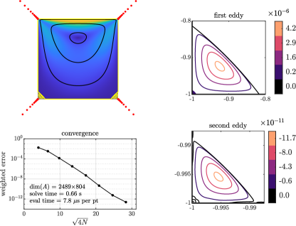
Figure 1: Stokes flow in a square lid-driven cavity computed to $12$-digit accuracy in half a second on a laptop. Stream contours and velocity magnitude (top left), convergence (bottom left), and close-ups of the first two Moffatt eddies in the lower-left corner (right). The red dots mark the exponentially clustered poles $(\ref{eq:allpoles})$ of the lightning approximation, $49$ at each upper corner and $39$ at each lower corner (with $4$ poles outside the plotting axes at each corner).

In this section and section 7 we illustrate the lightning Stokes solver applied to various model problems. Each example presents a contour plot of the stream function $\psi$ superimposed on a color plot of the velocity magnitude $\sqrt{u^{2}+v^{2}}$, using black contours for the main flow and yellow for the Moffatt eddies. The poles $\beta_{kn}$ are marked by red dots. As shown by plots in Examples 1 and 3, all the computations exhibit root-exponential convergence as a function of $4N$, the number of real degrees of freedom, as expected from the theory of [13]. The error measure in the plots is the maximum of the pointwise deviation from the boundary conditions weighted by distance to the nearest corner.

In standard floating point arithmetic, we can often get 10–12 digits of accuracy in $\psi$ with 20–40 poles clustered at each corner. In this regime the floating point limits are beginning to matter, and we have hand-tuned a few parameters to get the desired accuracy. Because of the root-exponential convergence, on the other hand, one can achieve 5–6 digits of accuracy with only 5–10 poles at each corner, with a reduction in linear algebra costs in principle by a factor of $1/16$ or better depending on details of boundary sampling and adaptivity. (In practice it is usually less because the computations are not in the asymptotic regime.) These lower-accuracy computations are easy, typically requiring no adaptivity or careful tuning of parameters.

Example 1. Lid-driven square cavity. Figure 1 presents a square lid-driven cavity, where the fluid is enclosed between solid walls one of which moves tangentially at speed 1 [34]. The domain is $\Omega=[-1,1]^{2}$, with boundary conditions $\psi=0$, $\psi_{n}=1$ on the top and $\psi=\psi_{n}=0$ on the other three sides. Since $\psi_{n}$ is discontinuous at the top corners, $\psi$ has singularities there. At the bottom corners there are weaker singularities associated with the formation of Moffatt eddies, but $\psi_{n}$ is continuous, and our adaptive strategy puts fewer poles at these corners.

The plots on the right in Figure 1 show close-ups of two eddies from the lower-left corner of the flow domain, with contours in each case at levels 0, 0.05, 0.35, 0.65, and 0.95 relative to the maximum value of $|\psi|$. Clearly the lightning method does a successful job of resolving two eddies, even though the stream function in the second one has amplitude of order $10^{-10}$. The eddies have the same shapes (on different space scales), opposite signs, and enormously different amplitudes.

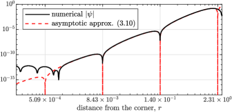
Figure 2: Log-log plot of the stream function magnitude $|\psi|$ along the diagonal of the lid-driven cavity. The computed stream function matches the asymptotic approximation $(\ref{eq:asymp})$ over an amplitude range of ten orders of magnitude. The constant $A_{0}$ of $(\ref{eq:asymp})$ was determined by least-squares fitting.

Note that the Moffatt eddies have the same forms in the lower-left and lower-right corners. In this as in all Stokes flows, reversing the signs of the boundary data just reverses the direction of the flow, since (1) is linear. In other words it doesn’t matter whether the lid is moving from left to right or right to left. This reversibility does not hold in Navier–Stokes flows, with nonzero Reynolds number and a nonlinear governing partial differential equation.

Figure 2 illustrates the power of asymptotic analysis, and the accuracy of the lightning solver, with a plot of $|\psi|$ along the $45^{\circ}$ line from the lower-left corner. The numerical results, displayed by the solid line, are compared with an asymptotic estimate based on (14). To obtain this estimate, we first calculated the complex eigenvalue $\lambda\approx 3.740+1.119\kern 0.3pti$ from (15) with $2\alpha=90^{\circ}$, and the complex constant $A_{0}$ of (14) was then determined by least-squares fitting of the $|\psi|$ data over the interval from the corner to the boundary between the eddies and the main flow. The curves show agreement of numerics with the asymptotic theory to about 12 digits.

These lightning calculations can be quite simple. The appendix illustrates this with a MATLAB code for the solution of the lid-driven cavity problem with 24 poles fixed near each corner and a polynomial of degree $24$ (Figure 11); this runs in 0.2 s on the same laptop and computes $\psi(0)\approx 0.11790231118443$ with an error of $1.7\times 10^{-13}$. If 24 is reduced to 6, the time is 0.04 s and the error is $4.8\times 10^{-7}$. For this geometry, the polynomial term is not very important to the solution: if its degree is reduced to 0, the errors increase only slightly to $6.2\times 10^{-12}$ and $7.4\times 10^{-7}$.

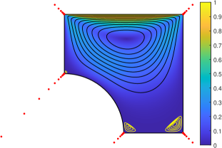
Figure 3: Lid-driven cavity with a quarter-circular exclusion, with $\psi$ calculated to $8$ digits in $0.3$ seconds.

Example 2. Lid-driven cavity with circular exclusion. A second lid-driven cavity is shown in Figure 3, now with a quarter-circular arc removed from the boundary. The computation is similar, and with polynomial degree $40$ and $20$ poles at each of the three corners, we get the value $\psi(0)\approx-0.0599323802$ to accuracy $6\times 10^{-9}$ in $0.3$ s.

Example 3. Lid-driven triangular cavity. Our third example, shown in Figure 4, is an isoceles triangle with unit side length and vertex angle $2\alpha=28.5^{\circ}$, corresponding to the complex eigenvalue $\lambda=9.485+4.434i$ in (15). The stream function is resolved to about 10 digits in half a second. The sharper corner makes the eddies decrease more slowly than before, with the ratio of successive amplitudes $|\psi|$ now about $830$. Three eddies can be observed without the need of a close-up.

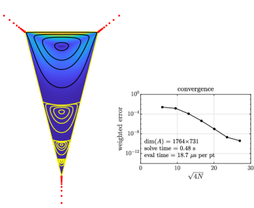
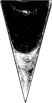
Figure 4: Stokes flow in a triangular lid-driven cavity of vertex angle $2\alpha=28.5^{\circ}$. There are $49$ poles at each corner, of which $7$ at the lower corner and $5$ at each upper corner lie outside the plotting axes. The computed result matches Taneda’s experiment from $1979$ [35].

This particular setup was chosen for comparison with experimental images from Taneda [35], which are well known from Van Dyke’s Album of Fluid Motion [41]. In his experiment, Taneda drove a flow of silicone oil at Reynolds number $0.17$ by a rotating cylinder, with flow visualization by aluminum powder and a photographic exposure time of 90 minutes. Only one Moffatt eddy is clearly visible in the experiment, as the velocities are nearly zero close to the corner. According to Taneda, “the reason is that the relative intensity of successive vortices is the order $10^{3}$, and therefore the photographic exposure necessary to visualize two successive vortices is about $10^{3}$ times that necessary to visualize a single vortex.” As far back as 1988, Rønquist successfully computed Taneda’s flow to a similar accuracy as ours using spectral element methods: 30 elements, each of order 8 [32, Fig. 12].

A comparison of the numerical results with the asymptotic approximation (14) as in Figure 2 (not shown) again indicates close agreement down to $|\psi|\approx 10^{-12}$.

6 Behavior outside the problem domain

Finite difference and finite element methods represent the solution to a PDE directly in the problem domain $\Omega$, and integral equations methods represent it via density functions supported on the boundary $\partial\kern 0.5pt\Omega$. In neither case is anything computed outside $\Omega$. Rational approximation methods, however, represent the solution by a function that is defined throughout the plane. In regions of analyticity, the computed approximation will typically provide an accurate analytic continuation across the boundary, whereas near branch points, it will feature a string of poles outside $\Omega$ that approximate a branch cut. For discussions of these effects see the conclusions section of [13] and Figure 3.2 of [29].

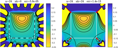
Figure 5: Approximations to the real function $\psi(z)$ for the lid-driven unit square cavity shown in the larger square $[-1.7,1.7]^{2}$. On the left, a degree $24$ polynomial approximation, and on the right, a rational approximation with, in addition, $24$ poles near each corner. The strings of poles approximate branch cuts needed to approximate the Goursat functions $f$ and $g$. The cavity boundary, marked in white, does not show up as a zero contour on the sides and the bottom because $\psi$ has a local minimum or maximum there rather than a change of sign.

For illustration, consider the biharmonic equation in the lid-driven square cavity. First, Figure 5 plots the computed approximation to the real function $\psi(z)$, not just on $\Omega$ itself but on the larger square $[-1.7,1.7]^{2}$. (In contrast to our other plots, here the colors represent $\psi$, not $\sqrt{u^{2}+v^{2}}$.) he image on the left shows a degree $24$ polynomial approximation, with the familiar circus tent effect at larger values of $|z|$. Such approximations are good for getting a few digits of accuracy, at least away from singular corners, and the error figure in the title reports 4-digit accuracy of the quantity $\psi(0)\approx-0.11790231118443$. However, convergence will be very slow as the degree is increased. The image on the right shows the result when $24$ poles are also included clustered near each corner. Now $\psi(0)$ is accurate to 13 digits, and the contours give some insight into how this is achieved. Although the functions $f$ and $g$ from which $\psi$ is derived have branch points at all four corners, good approximations interior to $\Omega$ are found thanks to the clustered poles. Note that the sides and the bottom of $\partial\kern 0.5pt\Omega$, marked in white, do not show up as black contours at level $\psi=0$. This is because $\psi$ has a local maximum rather than a simple zero there (or a minimum, inside the Moffatt eddy), which goes undetected by MATLAB’s contour finding algorithm. By contrast the separation lines between the main flow and the Moffatt eddies represent sign changes and do appear in black.

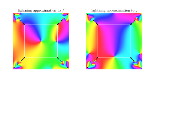
Figure 6: Phase portraits of the computed approximations to $f$ and $g$ in the same situation as the right image of Figure 5, with $24$ clustered poles at each corner (now marked in black rather than red). The approximations to both $f$ and $g$ show approximate branch cuts at the upper corners. The singularities at the lower corners are weaker.

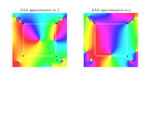
Figure 7: Phase portraits of AAA approximations with tolerance $10^{-8}$ to the functions of Figure 6. The poles are determined adaptively by the AAA algorithm and appear clustered near the corners, with $17$–$18$ poles near each upper corner and just $4$–$5$ poles near each lower corner, where the singularities are weaker.

To see more, we can examine the analytic functions $f$ and $g$ from which $\psi$ is constructed. Figure 6 shows phase portraits [42], with each pixel colored according to the phase of the function value there: red, yellow, green, cyan, blue, magenta for phases $0,\pi/3,2\pi/3,\dots,5\pi/3$. Perhaps the first thing one notices in these images is that $f$ has a zero at $z=0$. This is not important, being just a result of our normalization. The second feature one notices is the important one, that the approximations to $f$ and $g$ both show what look like branch cuts emanating from the upper corners. This is a familiar effect in rational approximation, and it illustrates why it is important for poles to be placed near these corners. One cannot say that the exact functions $f$ and $g$ themselves have branch cuts, for they are only defined on the unit square. But clearly they have branch points at $(1,1)$ and $(-1,1)$. They also have branch points at the lower corners, but these are weaker and not visible in the images.

In Figure 6, the poles are situated exactly where we placed them according to (18), with 24 poles at each corner. Now that we have good approximations to $f$ and $g$ on $\partial\kern 0.5pt\Omega$, however (hence also on $\Omega$ by the maximum modulus principle), it is possible to re-approximate these functions by new rational functions with free poles and see what structures emerge. Figure 7 shows what happens when this is done by AAA approximation [28] with a tolerance of $10^{-8}$. Although the poles have not been fixed in advance, we nevertheless find $17$ or $18$ poles clustering exponentially near each upper corner, for both $f$ and $g$. At the lower corners in this experiment, $f$ has 4 poles and $g$ has 5. These configurations confirm that the lightning method does a good job of capturing the true structure of the singularities of $f$ and $g$, and that there are singularities at all four corners but the lower ones are weaker.

7 Examples: channel flows

We now show a pair of flows in channels as opposed to bounded cavities. Physically, the channels are infinite, and we approximate them on bounded computational domains by specifying the stream function upstream and downstream. For the best results here we found it effective to remove the row weighting but scale all the columns of $A$ to have equal 2-norms.

Example 4. Square step. Figure 8 shows the flow over a square step, with the reentrant corner at $(0,0)$ and the salient corner at $(0,-1)$. Our computational domain introduces additional upstream corners at $(-2,0)$ and $(-2,1)$ and downstream corners at $(4,-1)$ and $(4,1)$. (As always, thanks to reversibility of Stokes flow, there is no true distinction between upstream and downstream.) Fully-developed parabolic velocity profiles are imposed at the inflow and outflow such that mass flow is conserved, $(u,v)=(1-(2y-1)^{2},0)$ at $x=-2$ and $(u,v)=((1-y^{2})/2,0)$ at $x=4$. That is, the stream function values are $\psi(-2,y)=2y^{2}-(4/3)y^{3}$ at the inflow and $\psi(4,y)=1/3+y/2-y^{3}/6$ at the outflow, and we complete the boundary conditions by specifying $\psi_{0}=2/3$ on the top of the channel, $\psi_{0}=0$ on the bottom, and $\psi_{n}=0$ everywhere. We normalize the Goursat functions by $f(0.5)=0$, $\hbox{\rm Re\kern 0.3pt}\kern 0.7ptg(0.5)=0$, and $\hbox{\rm Re\kern 0.3pt}f(1)=0$.

Figure 8 was generated by a code with polynomial degree $40$ and $80$ poles clustered at the reentrant corner. The computation runs in about 0.6 s on our laptop and computes $\psi(z)$ to about 6 digits of accuracy: for $z=1,2,3$ the computed values are $0.259289$, $0.329814$, and $0.333990$. (It surprised us that this last number could be greater than the centerline value of $1/3$, but this seems to be genuine. If the length of the computational domain is increased to better approximate an infinite channel, $\psi(3)$ increases slightly to $0.334054$.)

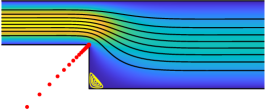
Figure 8: Stokes flow over a step, with the infinite channel approximated by a finite domain with explicit inflow and outflow conditions.

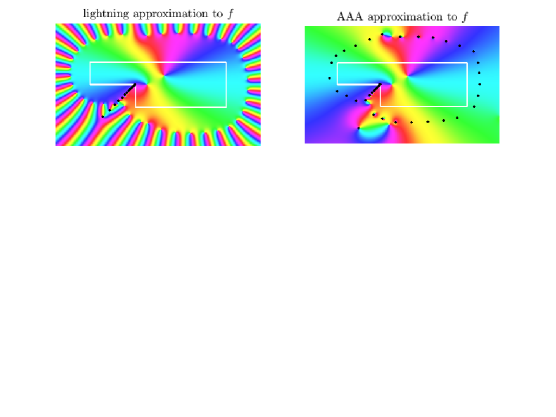
Figure 9: Phase portraits of the Goursat function $f$ for the flow over a step and of its AAA rational approximation with tolerance $10^{-8}$. The black dots marking poles confirm that only the reentrant corner has a signiciant singularity.

Following Figure 7, Figure 9 shows phase portraits of the lightning approximation to the Goursat function $f$ for flow over the step, and its AAA approximant with tolerance $10^{-8}$.

Example 5. Bent channel. Figure 10 shows a flow in a smooth channel with a bend in it: the upper boundary is $y=1/2-\tanh(3(x+.2))/2$ and the lower boundary is the same curve rotated by $\pi$. Since the walls are smooth, we use a purely polynomial expansion of degree $n=300$. The speed of flow is $1$ in the middle of the channel at inflow and outflow, and at the center point $z=0$ the computation gives speed $1.072187183679$, as compared with the true value of about $1.072187183704$.

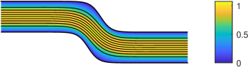
Figure 10: Stokes flow in a smooth bent channel, computed to $10$-digit accuracy by a polynomial expansion of degree $300$.

8 Discussion

The association of biharmonic functions and Stokes flow with analytic functions goes back to the beginnings of these subjects, and in various forms it has served as the basis of computations, though perhaps not as frequently as one might have expected. For example, a stokeslet is a biharmonic function with a point singularity [7, 16, 21], and superpositions of stokeslets have been used for numerical computations [6, 9, 22]. What is distinctive about the lightning approach to these problems is the use of strings of singularities exponentially clustered near corners. This leads to root-exponential convergence with respect to the number of free parameters [13, 40], an effect first identified in rational approximation theory by Newman in 1964 [30]. With analysis of the singular behavior at each corner, one could develop methods for certain problems with even faster exponential convergence, but that requires case-by-case analysis. A more general approach to increasing convergence rates, the “log-lightning” method based on reciprocal-log approximations [29], has not yet been investigated for biharmonic problems.

The advantages of the lightning method are its simplicity, its great speed and accuracy, and the fact that it delivers a global representation of the solution (perfectly smooth and exactly biharmonic). A typical problem may be solved in less than a second, with the solution in the form of a function handle whose evaluation takes 5–50 microseconds per point. We also feel it is a worthwhile contribution conceptually, highlighting as it does the analyticity properties that are such a fundamental feature of these problems.

Following Goursat, our method explicitly constructs complex analytic functions $f$ and $g$. However, it has been known for a long time that there are alternative formulations involving real harmonic functions, associated with the names of Almansi and Krakowski and Charnes: here the representation $\hbox{\rm Im}\kern-0.8pt\left\{\overline{z}f(z)+g(z)\right\}$ of (4) becomes $h(z)+xk(z)$, $h(z)+yk(z)$, or $h(z)+r^{2}k(z)$, where $h$ and $k$ are real and harmonic and $r=|z|$ [10, 18, 33]. So far as we are aware, these representations could serve equally well as the basis of a lightning solver.

We see two drawbacks to the lightning method. One is that issues of numerical stability are never far away and only partially understood. The Vandermonde with Arnoldi orthogonalization we have described goes a good way to eliminating stability problems in many cases, enabling computed results sometimes with close to machine accuracy, but in other cases we find ourselves stuck at 10 digits or less. We hope that further investigation will lead to better undertanding and consequent improvements, as indeed happened in the case of the original lightning Laplace method, which was presented in [13] before the introduction of Vandermonde with Arnoldi [3].

The other drawback is one that arises widely in computations based on complex analysis, which is related to the “crowding phenomenon” in numerical conformal mapping [14, Thms. 2–5]. Though the theorems may tell us that exponentially clustered poles at each singularity ensure root-exponential convergence, the constants associated with the remaining, analytic part of the problem may be quite adverse for domains involving certain distortions. To combat such effects one may employ representations of the Goursat functions $f$ and $g$ that go beyond the basic prescription of clustered poles + polynomial, and this is a matter for further investigation. It may prove fruitful to develop a variant of our algorithm that combines exponentially clustered poles near singularities with non-clustered poles spaced along curves, as in the more usual method of fundamental solutions [17, 18, 33]. Indeed, the distribution of poles in the AAA approximation on the right of Figure 9 seems to point in this direction.

The geometries we have considered here have been limited, but we believe closely related methods will work for other cases too. One prospect would be truly unbounded domains, such as infinite channels, treated without artificial inflow and outflow conditions. Complex variables and rational functions generally cope with unbounded domains easily, so we are confident that this kind of problem should be accessible. Multiply-connected domains should also be treatable without great changes. At first this may seem daunting, since the Goursat functions $f$ and $g$ will have to be multi-valued [10], but in fact just a single complex logarithm will be needed in each hole, as pointed out by Axler in his wonderfully clear discussion of the “logarithmic conjugation theorem” [1]. Series methods for Laplace problems with smooth holes are considered in [37], and holes with corners and lightning terms appear in [39]. A third geometrical variation could be problems with free boundaries [31, sec. 3.5]. And, of course, one may treat problems of elasticity as well as fluid mechanics.

Extension of these methods to three dimensions is undoubtedly possible, but not straightforward, and we have no view as to whether something practical can be developed here or not.

For 2D Laplace problems, a lightning solver is available as a MATLAB code that treats a wide variety of problems with a simple interface [38]. At present there is no comparable software for the biharmonic case, so prospective users of this method are recommended to begin by adapting the codes listed in the appendix.

Appendix

      % Setup
        w = [1+1i; -1+1i; -1-1i; 1-1i];               % corners
        m = 300; s = tanh(linspace(-16,16,m));        % clustered pts in (-1,1)
        Z = [1i-s -1-1i*s -1i+s 1+1i*s].’;            % boundary pts
        top = 1:m; lft = m+1:2*m; bot = 2*m+1:3*m;    % indices
        rgt = 3*m+1:4*m; sid = [lft rgt];
        n = 24; np = 24;                              % poly. deg.; # poles per corner
        dk = 1.5*cluster(np); d1 = 1+dk;              % tapered exponential clustering
        Pol = {w(1)*d1, w(2)*d1, w(3)*d1, w(4)*d1};   % the poles
        Hes = VAorthog(Z,n,Pol);                      % Arnoldi Hessenberg matrices

      % Boundary conditions
        [A1,rhs1,A2,rhs2,PSI,U,V] = makerows(Z,n,Hes,Pol);
        A1(top,:) = PSI(top,:); rhs1(top) = 0;        % Top:    psi = 0,
        A2(top,:) =   U(top,:); rhs2(top) = 1;        %         U = 1
        A1(bot,:) = PSI(bot,:); rhs1(bot) = 0;        % Bottom: psi = 0,
        A2(bot,:) =   U(bot,:); rhs2(bot) = 0;        %         U = 0
        A1(sid,:) = PSI(sid,:); rhs1(sid) = 0;        % Sides:  psi = 0,
        A2(sid,:) =   V(sid,:); rhs2(sid) = 0;        %         V = 0
        A = [A1; A2]; rhs = [rhs1; rhs2];             % put the halves together

      % Solution and plot
        [A,rhs] = rowweighting(A,rhs,Z,w);            % row weighting (optional)
        [A,rhs] = normalize(A,rhs,0,1,Hes,Pol);       % normalize f and g (optional)
        c = A\rhs;                                    % solve least-squares problem
        [psi,uv,p,omega,f,g] = makefuns(c,Hes,Pol);   % make function handles
        plotcontours(w,Z,psi,uv,Pol)                  % contour plot
        ss = ’Error in psi(0) = %6.1e\n’;
        fprintf(ss,psi(0)+.117902311184435)           % accuracy check

Figure 11: MATLAB program for the lid-driven square cavity, an example of a ten digit algorithm as defined in [36]. This code computes the solution accurate to $13$ digits (as measured by $\psi(0)$) in $0.2$ secs on a laptop and produces a plot in a further $3.5$ secs. It calls the functions VAorthog and VAeval listed in Figure 12 for Vandermonde with Arnoldi orthogonalization and the functions listed in Figures 13 and 14 for the remaining computation and plotting.

The method we have presented can be realized in short MATLAB codes. As a template, Figure 11 presents an example for the square lid-driven cavity, which readers may adapt to their own problems. This code calls a pair of functions for Vandermonde with Arnoldi orthogonalization, shown in Figure 12, and additional functions for setting up the algorithm and plotting, shown in Figures 13 and 14.

     function [Hes,R] = VAorthog(Z,n,varargin)  % Vand.+Arnoldi orthogonalization
     %  Input:   Z = column vector of sample points
     %           n = degree of polynomial (>= 0)
     %         Pol = cell array of vectors of poles (optional)
     % Output: Hes = cell array of Hessenberg matrices (length 1+length(Pol))
     %           R = matrix of basis vectors
     M = length(Z); Pol = []; if nargin == 3, Pol = varargin{1}; end
     % First orthogonalize the polynomial part
     Q = ones(M,1); H = zeros(n+1,n);
     for k = 1:n
        q = Z.*Q(:,k);
        for j = 1:k, H(j,k) = Q(:,j)’*q/M; q = q - H(j,k)*Q(:,j); end
        H(k+1,k) = norm(q)/sqrt(M); Q(:,k+1) = q/H(k+1,k);
     end
     Hes{1} = H; R = Q;
     % Next orthogonalize the pole parts, if any
     while ~isempty(Pol)
        pol = Pol{1}; Pol(1) = [];
        np = length(pol); H = zeros(np,np-1); Q = ones(M,1);
        for k = 1:np
           q = Q(:,k)./(Z-pol(k));
           for j = 1:k, H(j,k) = Q(:,j)’*q/M; q = q - H(j,k)*Q(:,j); end
           H(k+1,k) = norm(q)/sqrt(M); Q(:,k+1) = q/H(k+1,k);
        end
        Hes{length(Hes)+1} = H; R = [R Q(:,2:end)];
     end

     function [R0,R1] = VAeval(Z,Hes,varargin)  % Vand.+Arnoldi basis construction
     %  Input:   Z = column vector of sample points
     %         Hes = cell array of Hessenberg matrices
     %         Pol = cell array of vectors of poles, if any
     % Output:  R0 = matrix of basis vectors for functions
     %          R1 = matrix of basis vectors for derivatives
     M = length(Z); Pol = []; if nargin == 3, Pol = varargin{1}; end
     % First construct the polynomial part of the basis
     H = Hes{1}; Hes(1) = []; n = size(H,2);
     Q = ones(M,1); D = zeros(M,1);
     for k = 1:n
        hkk = H(k+1,k);
        Q(:,k+1) = ( Z.*Q(:,k) - Q(:,1:k)*H(1:k,k)          )/hkk;
        D(:,k+1) = ( Z.*D(:,k) - D(:,1:k)*H(1:k,k) + Q(:,k) )/hkk;
     end
     R0 = Q; R1 = D;
     % Next construct the pole parts of the basis, if any
     while ~isempty(Pol)
        pol = Pol{1}; Pol(1) = [];
        H = Hes{1}; Hes(1) = []; np = length(pol); Q = ones(M,1); D = zeros(M,1);
        for k = 1:np
           Zpki = 1./(Z-pol(k)); hkk = H(k+1,k);
           Q(:,k+1) = ( Q(:,k).*Zpki - Q(:,1:k)*H(1:k,k)                   )/hkk;
           D(:,k+1) = ( D(:,k).*Zpki - D(:,1:k)*H(1:k,k) - Q(:,k).*Zpki.^2 )/hkk;
        end
        R0 = [R0 Q(:,2:end)]; R1 = [R1 D(:,2:end)];
     end

Figure 12: MATLAB codes for Vandermonde with Arnoldi orthogonalization and evaluation, adapted from [3]. The polynomial part and each string of poles are orthogonalized separately, with the resulting Hessenberg matrices of coefficients stored in the cell array Hes.

     function d = cluster(n)   % n points exponentially clustered in (0,1]
     nc = ceil(n); d = exp(4*(sqrt(nc:-1:1)-sqrt(nc)));

     function [A1,rhs1,A2,rhs2,PSI,U,V] = makerows(Z,n,Hes,varargin)
     Pol = []; if nargin == 4, Pol = varargin{1}; end
     [R0,R1] = VAeval(Z,Hes,Pol);
     M = length(Z); N = 4*size(R0,2);
     cZ = spdiags(conj(Z),0,M,M);                    % conj(Z)
     PSI = [cZ*R0 R0]; PSI = [imag(PSI) real(PSI)];  % eq (2.1): stream function
     U = [cZ*R1-R0 R1]; U = [real(U) -imag(U)];      % eq (3.9): horizontal velocity
     V = [-cZ*R1-R0 -R1]; V = [imag(V) real(V)];     % eq (3.9): vertical velocity
     A1 = zeros(M,N); rhs1 = zeros(M,1);
     A2 = zeros(M,N); rhs2 = zeros(M,1);

     function [A,rhs] = normalize(A,rhs,a,b,Hes,varargin)
     % Impose conditions at z=a and z=b to make f and g unique
     Pol = []; if nargin == 6, Pol = varargin{1}; end
     rhs = [rhs; 0; 0; 0; 0];
     z = a; r0 = VAeval(z,Hes,Pol); zero = 0*r0;
     A = [A; real([r0 zero]) -imag([r0 zero])];      % Re(f(a)) = 0
     A = [A; imag([r0 zero])  real([r0 zero])];      % Im(f(a)) = 0
     A = [A; real([zero r0]) -imag([zero r0])];      % Re(g(a)) = 0
     z = b; r0 = VAeval(z,Hes,Pol);
     A = [A; real([r0 zero]) -imag([r0 zero])];      % Re(f(b)) = 0

     function [A,rhs] = rowweighting(A,rhs,Z,w)      % row weighting
     dZw = min(abs(Z-w.’),[],2);                     % distance to nearest corner
     wt = [dZw; dZw];
     M2 = 2*length(Z); W = spdiags(wt,0,M2,M2);
     A = W*A; rhs = W*rhs;

     function [psi,uv,p,omega,f,g] = makefuns(c,Hes,varargin)  % make function handles
     Pol = []; if nargin == 3, Pol = varargin{1}; end
     cc = c(1:end/2) + 1i*c(end/2+1:end);
     reshaper = @(str) @(z) reshape(fh(str,z(:),cc,Hes,Pol),size(z));
       psi = reshaper(’psi’);    uv = reshaper(’uv’);   p = reshaper(’p’);
     omega = reshaper(’omega’);   f = reshaper(’f’);    g = reshaper(’g’);

     function fh = fh(i,Z,cc,Hes,Pol)
     [R0,R1] = VAeval(Z,Hes,Pol);
     N = size(R0,2);
     cf = cc(1:N); cg = cc(N+(1:N));
     switch i
        case   ’f’  , fh = R0*cf;                                % eq (4.1): f
        case   ’g’  , fh = R0*cg;                                % eq (4.1): g
        case  ’psi’ , fh = imag(conj(Z).*(R0*cf) + R0*cg);       % eq (2.1): psi
        case   ’uv’ , fh = Z.*conj(R1*cf) - R0*cf + conj(R1*cg); % eq (3.7): u+1i*v
        case   ’p’  , fh = real(4*R1*cf);                        % eq (3.8): pressure
        case ’omega’, fh = imag(-4*R1*cf);                       % eq (3.8): vorticity
     end

Figure 13: Stokes discretization codes.

     function plotcontours(w,Z,psi,uv,varargin)   % contour plot
     Pol = []; if nargin == 5, Pol = varargin{1}; end
     MS = ’markersize’; LW = ’linewidth’; CO = ’color’;
     x1 = min(real(Z)); x2 = max(real(Z)); xm = mean([x1 x2]); dx = diff([x1 x2]);
     y1 = min(imag(Z)); y2 = max(imag(Z)); ym = mean([y1 y2]); dy = diff([y1 y2]);
     dmax = max(dx,dy); nx = ceil(200*dx/dmax); ny = ceil(200*dy/dmax);
     x = linspace(x1,x2,nx); y = linspace(y1,y2,ny);
     [xx,yy] = meshgrid(x,y); zz = xx + 1i*yy;
     inpolygonc = @(z,w) inpolygon(real(z),imag(z),real(w),imag(w));
     dZw = min(abs(Z-w.’),[],2);  % distance to nearest corner
     ii = find(dZw>5e-3); outside = ~inpolygonc(zz,Z(ii));
     uu = abs(uv(zz)); uu(outside) = NaN; umax = max(max(uu));
     pcolor(x,y,uu), hold on, colormap(gca,parula)
     shading interp, colorbar, caxis([0 umax])
     plot(Z([1:end 1]),’k’,LW,.8)
     pp = psi(zz); pp(outside) = NaN; pmin = min(min(pp)); pmax = max(max(pp));
     lev = pmin+(.1:.1:.9)*(pmax-pmin);
     contour(x,y,pp,lev,’k’,LW,.6)
     psiratio = pmin/pmax; fac = max(psiratio,1/psiratio);
     if sign(fac) == -1     % Moffatt eddies in yellow
        lev1 = lev(1:2:end)*fac;
        contour(x,y,pp,lev1,’y’,LW,.55)
        if abs(fac) > 1e4   % second eddies (white)
           lev2 = lev1*fac; contour(x,y,pp,lev2,LW,.5,CO,.99*[1 1 1])
        end
        if abs(fac) > 1e3   % third eddies (yellow)
           lev3 = lev2*fac; contour(x,y,pp,lev3,’y’,LW,.45)
        end
     end
     if nargin==5, plot(cell2mat(Pol),’.r’,MS,8), end
     hold off, axis([xm+.6*dx*[-1 1] ym+.6*dy*[-1 1]]), axis equal off

Figure 14: Contour plotter.

References

- [1] S. Axler, Harmonic functions from a complex analysis viewpoint, Amer. Math. Monthly, 93 (1986), pp. 246–258.
- [2] R. Becker and S. Mao, Quasi-optimality of adaptive nonconforming finite element methods for the Stokes equations, SIAM J. Numer. Anal., 49 (2011), pp. 970–991.
- [3] P. D. Brubeck, Y. Nakatsukasa, and L. N. Trefethen, Vandermonde with Arnoldi, SIAM Rev., to appear.
- [4] G. F. Carrier, M. Krook, and C. E. Pearson, Functions of a Complex Variable: Theory and Technique, SIAM, 2005.
- [5] C. Carstensen, D. Peterseim, and H. Rabus, Optimal adaptive nonconforming FEM for the Stokes problem, Numer. Math., 123 (2013), pp. 291–308.
- [6] R. Cortez, The method of regularized Stokeslets, SIAM J. Sci. Comput., 23 (2001), pp. 1204–1225.
- [7] J. Dauparas and E. Lauga, Leading-order Stokes flows near a corner, IMA J. Appl. Math., 83 (2018), pp. 590–633.
- [8] W. R. Dean and P. E. Montagnon, On the steady motion of viscous liquid in a corner, Math. Proc. Cambridge Phil. Soc., 45 (1949), pp. 389–394.
- [9] M. D. Finn, S. M. Cox, and H. M. Byrne, Topological chaos in inviscid and viscous mixers, J. Fluid Mech., 493 (2003), pp. 345–361.
- [10] R. L. Fosdick, On the complete representation of biharmonic functions, SIAM J. Appl. Math., 19 (1970), pp. 243–250.
- [11] J. N. Goodier, An analogy between the slow motions of a viscous fluid in two dimensions, and systems of plane stress, Philos. Mag., 17 (1934), pp. 554–576.
- [12] A. Gopal and L. N. Trefethen, New Laplace and Helmholtz solvers, Proc. Natl. Acad. Sci., 116 (2019), pp. 10223–10225.
- [13] A. Gopal and L. N. Trefethen, Solving Laplace problems with corner singularities via rational functions, SIAM J. Numer. Anal., 57 (2019), pp. 2074–2094.
- [14] A. Gopal and L. N. Trefethen, Representation of conformal maps by rational functions, Numer. Math. 142 (2019), pp. 359–382.
- [15] E. Goursat, Sur l’équation , Bull. Soc. Math. France, 26 (1898), pp. 236–237.
- [16] H. Hasimoto and O. Sano, Stokeslets and eddies in creeping flow, Ann. Rev. Fluid Mech., 12 (1980), pp. 335–363.
- [17] A. Karageorghis and G. Fairweather, The method of fundamental solutions for the numerical solution of the biharmonic equation, J. Comp. Phys., 69 (1987), pp. 434–459.
- [18] A. Karageorghis and G. Fairweather, The Almansi method of fundamental solutions for solving biharmonic problems, Int. J. Numer. Meth. Engr., 26 (1988), pp. 1665–1682.
- [19] A. O. Kazakova and A. G. Petrov, Computation of viscous flow between two arbitrarily moving cylinders of arbitrary cross section, Comp. Math. Math. Phys., 59 (2019), pp. 1030–1048.
- [20] Y. Kondratyuk and R. Stevenson, An optimal adaptive finite element method for the Stokes problem, SIAM J. Numer. Anal., 46 (2008), pp. 747–775.
- [21] W. E. Langlois and M. O. Deville, Slow Viscous Flow, 2nd ed., Springer, 2014.
- [22] E. Lauga and T. R. Powers, The hydrodynamics of swimming microorganisms, Rep. Prog. Phys., 72 (2009), 096601.
- [23] E. Luca and D. G. Crowdy, A transform method for the biharmonic equation in multiply connected circular domains, IMA J. Appl. Math., 83 (2018), pp. 942–976.
- [24] E. Luca and S. G. Llewellyn Smith, Stokes flow through a two-dimensional channel with a linear expansion, Quart. J. Mech. Appl. Math., 71 (2018), pp. 441–462.
- [25] H. K. Moffatt, Viscous and resistive eddies near a sharp corner, J. Fluid Mech., 18 (1964), pp. 1–18.
- [26] N. I. Muskhelishvili, Sur l’integration de l’équation biharmonique, Bull. Acad. Sci. Russ., 13 (1919), pp. 663–686.
- [27] N. I. Muskhelishvili, Some Basic Problems of the Mathematical Theory of Elasticity, Springer, 1977.
- [28] Y. Nakatsukasa, O. Sète, and L. N. Trefethen, The AAA algorithm for rational approximation, SIAM J. Sci. Comp., 40 (2018), pp. A1494–A1522.
- [29] Y. Nakatsukasa and L. N. Trefethen, Reciprocal-log approximation and planar PDE solvers, SIAM J. Numer. Anal., submitted, 2020.
- [30] D. J. Newman, Rational approximation to , Michigan Math. J., 11 (1964), pp. 11–14.
- [31] H. Ockendon and J. R. Ockendon, Viscous Flow, Cambridge U. Press, 1995.
- [32] E. M. Rønquist, Optimal Spectral Element Methods for the Unsteady Three-Dimensional Incompressible Navier–Stokes Equations, PhD thesis, MIT, 1988.
- [33] K. Sakakibara, Method of fundamental solutions for biharmonic equation based on Almansi-type decomposition, Applications of Mathematics, 62 (2017), pp. 297–317.
- [34] P. N. Shankar and M. D. Deshpande, Fluid mechanics in the driven cavity, Ann. Rev. Fluid Mech., 32 (2000), pp. 93–136.
- [35] S. Taneda, Visualization of separating Stokes flows, J. Phys. Soc. Japan, 46 (1979), pp. 1935–1942.
- [36] L. N. Trefethen, Ten digit algorithms, Numer. Anal. Rep. 05/13, University of Oxford, 2005; available at people.maths.ox.ac.uk/trefethen/papers.html.
- [37] L. N. Trefethen, Series solution of Laplace problems, ANZIAM J., 60 (2018), pp. 1–26.
- [38] L. N. Trefethen, Lightning Laplace code laplace.m, people.maths.ox.ac.uk/trefethen/ laplace, 2020.
- [39] L. N. Trefethen, Numerical conformal mapping with rational functions, Comp. Meth Funct.. Th., 2020.
- [40] L. N. Trefethen, Y. Nakatsukasa, and J. A. C. Weideman, Exponential node clustering at singularities for rational approximation, quadrature, and PDEs, Numer. Math., 2021.
- [41] M. Van Dyke, An Album of Fluid Motion, Parabolic Press, Stanford, 1982.
- [42] E. Wegert, Visual Complex Functions: An Introduction with Phase Portraits, Birkhäuser, 2012.