Learning Hierarchical Graph Neural Networks for Image Clustering

Abstract

We propose a hierarchical graph neural network (GNN) model that learns how to cluster a set of images into an unknown number of identities using a training set of images annotated with labels belonging to a disjoint set of identities. Our hierarchical GNN uses a novel approach to merge connected components predicted at each level of the hierarchy to form a new graph at the next level. Unlike fully unsupervised hierarchical clustering, the choice of grouping and complexity criteria stems naturally from supervision in the training set. The resulting method, Hi-LANDER, achieves an average of 54% improvement in F-score and 8% increase in Normalized Mutual Information (NMI) relative to current GNN-based clustering algorithms. Additionally, state-of-the-art GNN-based methods rely on separate models to predict linkage probabilities and node densities as intermediate steps of the clustering process. In contrast, our unified framework achieves a seven-fold decrease in computational cost. We release our training and inference code here.

1 Introduction

Clustering is a pillar of unsupervised learning. It consists of grouping data points according to a manually specified criterion. Without any supervision, the problem is self-referential, with the outcome being defined by the choice of grouping criterion. Different criteria yield different solutions, with no independent validation mechanism. Even within a given criterion, clustering typically yields multiple solutions depending on a complexity measure, and a separate model selection criterion is introduced to arrive at a unique solution. A large branch of unsupervised clustering methods follow the hierarchical/agglomerative framework [44, 45, 48], which gives a tree of cluster partitions with varying granularity of the data, but they still require a model selection criterion for the final single grouping. Rather than engineering the complexity and grouping criteria, we wish to learn them from data. Clearly, this is not the data we wish to cluster, for we do not have any annotations for them. Instead, it is a different set of training data, the meta-training set, for which cluster labels are given, corresponding to identities that are disjoint from those expected in the test set. For example, the test set might be an untagged collection of photos by a particular user, for which there exists a true set of discrete identities that we wish to discover, say their family members. While those family members have never been seen before, the system has access to different photo collections, tagged with different identities, during training. Our goal is to leverage the latter labeled training set to learn how to cluster different test sets with unknown numbers of different identities. This is closely related to “open-set” or “open universe” classification [43, 27].

We present the first hierarchical/agglomerative clustering method using Graph Neural Networks (GNNs). GNNs are a natural tool for learning how to cluster [56, 62, 61], as they provide a way of predicting the connectivity of a graph using training data. In our case, the graph describes the connectivity among test data, with connected components ultimately determining the clusters.

Our hierarchical GNN uses a novel approach to merge connected components predicted at each level of the hierarchy to form a new graph at the next level. We employ a GNN to predict connectivity at each level, and iterate until convergence. While in unsupervised agglomerative clustering convergence occurs when all clusters are merged to a single node [45, 48], or when an arbitrary threshold of an arbitrary model complexity criterion is reached, in our case convergence is driven by the training set, and occurs when no more edges are added to the graph by the GNN. There is no need to define an arbitrary model selection criterion. Instead, the “natural granularity” of the clustering process is determined inductively, by the ground truth in the training set.

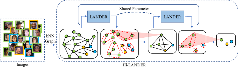
Figure 1: The proposed hierarchical clustering framework Hi-LANDER. Images are embedded into a $k$-NN graph with their visual features. The green, yellow and blue image boundaries illustrate that they belong to three different classes; same for the color of the graph nodes. At each level of the hierarchy, our base LANDER model outputs a set of selected edges and thus intermediate clusters. These clusters are then grouped into super-nodes as input for the next level. The process continues til convergence, i.e., when no more edges are added to the graph. Weights of LANDER are shared across multiple levels of the hierarchy. Best viewed in color.

Unlike prior clustering work using GNNs [56, 62, 61], we perform full-graph inference to jointly predict two attributes: linkage probabilities at the edges, and densities at the nodes, defined as the proportion of similar vertices that share the same label within a node’s neighborhood [14, 3, 61]. The densities establish a relative order between nodes [3, 61], which is then used to guide the connectivity. Nodes at the boundary between two ground-truth clusters, or nodes having a majority of their neighbors belonging to different classes, tend to have a low density, and accordingly a low expectation of linkage probability to their neighbors. Prior methods predict the edge connectivity as a node attribute on numerous sampled sub-graphs [56, 61]; ours directly infers the full graph and predicts connectivity as an attribute of the edges. Also, prior methods require separate models for the two attributes of linkage probabilities and node densities, whereas ours infers them jointly. This is beneficial as there is strong correlation between the two attributes, defined by the ground truth. A joint model also achieves superior efficiency, which enables hierarchical inference that would otherwise be intractable. Compared to the two separate models, we achieve a seven-fold speedup from 256s to 36s as shown in  Table 1.

In terms of accuracy, Our method achieves an average 54% improvement in F-score, from 0.391 to 0.604, and an average 8% increase in NMI, from 0.778 to 0.842 compared to state-of-art GNN based clustering methods [61, 56] over the face and species clustering benchmarks as shown in  Table 3. Furthermore, the pseudo-labels generated by our clustering of unlabeled data can be used as a regularization mechanism to reduce face verification error by 14%, as shown in Table 4, from 0.187 to 0.159 in compared to state-of-art clustering methods, allowing us to approach the performance of fully supervised training at 0.136.

In the next section, we summarize our contributions in the context of prior related work. In Section 3 we introduce the technical innovations of our paper, and in Section 4 we detail our experiment results. We discuss failure modes and limitations of our method in Section 5.

2 Related Work and Contributions

Unsupervised Visual Clustering Traditional unsupervised clustering algorithms utilize the notion of similarity between objects, such as K-means [28] and hierarchical agglomerative methods [34, 44, 40]. [5] extends Hierarchical Agglomerative Clustering (HAC) [44] with a distance based on node pair sampling probability. Approaches based on persistent-homology [66] and singular perturbation theory [35] deal with the scale-selection issue. [14, 3, 8] utilize a notion of density defined as the proportion of similar nodes within a neighborhood. Spectral clustering methods [35, 17, 51] approximate graph-cuts with a low-dimensional embedding of the affinity matrix via eigen-decomposition. Graclus [13] provides an alternative to spectral clustering with multi-level weighted graph cuts. H-DBSCAN [8] removes the distance threshold tuning in [14]. FINCH [42] proposes a first neighbor heuristic and generates a hierarchy of clusters. More recent unsupervised methods [24, 25] utilize deep CNN features. [65] proposes a Rank-Order distance measurement. Our hierarchical design relates the most to [42], however, instead of the heuristic to link the first-neighbor of each node for edge selection, which is prone to error and has limited capability in dealing with large-scale complex cluster structures, we use a learnable GNN model.

Supervised Visual Clustering Supervised graph neural network-based approaches [56, 62, 64, 62, 61] perform clustering on a $k$-NN graph. In contrast to these methods that produce only a single partition, our method generates a hierarchy of cluster partitions and deals with unseen complex cluster structures with a learnt convergence criterion from the natural granularity of the “meta-training” set. In contrast to [61] which requires two separate models to perform edge connectivity and node density estimation, our method jointly predicts these two quantities with a single model of higher accuracy and efficiency (Table 1). Furthermore, [56, 61] estimate linkage as a node attribute on sub-sampled graphs, whereas we estimate it as an edge attribute with natural parallelization through full-graph inference and significantly reduce runtime (Table 5). [1] uses a two-step process that first refines visual embeddings with a GNN and then runs a top-down divisive clustering, with testing limited to small datasets. In contrast, our method performs clustering as a graph edge selection procedure.

Hierarchical Representation Hierarchical structures have also been extensively studied in many visual recognition tasks [36, 22, 29, 58, 31, 15, 33, 23]. In this paper, our hierarchy is formed by multiple $k$-NN graphs recurrently built with clustering and node aggregation, which are learnt from the meta-training set. Hierarchical representation has also been explored in the graph representation learning literature [63, 9, 4, 19, 18, 26]. There, the focus is to learn a stronger feature representation to classify graph [63] or input nodes [18] into a closed set of class labels. Whereas, our goal is to “learn” to cluster from a meta-training set whose classes are disjoint to those of test-time.

Graph Neural Networks in Visual Understanding The expressive power of GNNs in dealing with complex graph structures is shown to benefit many visual learning tasks [21, 16, 10, 55, 49, 12, 59, 60, 11, 6, 57]. [16] samples and aggregates embeddings of neighboring nodes. [49] further advances [16] with additive attention. [10] uses a batch training scheme based on [16] to reduce computational cost. [55] performs node classification with edge convolution and feature aggregation through max-pooling. Our method differs from [55] in that we use a unified model that jointly learns node densities and edge linkages with two supervision signals. Furthermore, our GNN learns the edge selection and convergence criteria for a hierarchical agglomerative process.

Contributions We propose the first hierarchical structure in GNN-based clustering. Our method, partly inspired by [42], refines the graph into super-nodes formed by sub-clusters and recurrently runs the clustering on the super-node graphs, but differs in that we use a learnt GNN to predict sub-clusters at each recurrent step instead of an arbitrary manual grouping criterion. At convergence, we trace back the predicted cluster labels on the super-nodes from the top-level graph to the original data points to obtain the final cluster.

Our method converges to a cluster based on the level of granularity established by ground truth labels in the training set. Although the identities are different from the test set, they are sufficient to implicitly define a complexity criterion for the clustering at inference time, without the need for a separate model selection criterion.

To run multiple iterations of the GNN model efficiently and effectively, we design a base model that approximates label-aware linkage probabilities and densities of similar nodes that share the same label. The densities are useful for additional regularization and refining edge selection. We refer to this base model as our Link Approximation aNd Density Estimation Refinement (LANDER) module. Finally, we denote our hierarchical clustering method Hi-LANDER and  Figure 1 illustrates its structure.

The key innovation of our method is two-fold: 1) we produce a hierarchy of cluster partitions instead of a single flat partition of [62, 56, 61]; 2) We perform full-graph inference to jointly predict attributes of both nodes and edges, whereas prior GNN methods used sub-graph inference and separate models for node and edge attribute prediction. These innovations are collectively responsible for improving the clustering performance by an average of 54% F-score and 8% NMI over existing GNN-based methods.

3 Methodology

3.1 Clustering with a $k$-NN Graph

Formally, given a set of $N$ images $D=\{I_{i}\}_{i=1}^{N}$ and their corresponding visual embeddings $F=\{f_{i}\}_{i=1}^{N}$, we first construct an affinity graph $G=\{V,E\}$, where $|V|=N$, via $k$-nearest neighbors determined w.r.t. cosine similarity, i.e., the inner-product of the normalized visual embeddings. Each image (for example one face crop) entails one object to cluster and represents a node in the graph, with the node feature being its visual embedding $f_{i}$. The edges connect each node to its $k$ neighbors. Per the clustering paradigms in [14, 8, 3, 42, 56, 61, 37], a function $\phi$ takes as input the affinity graph $G$ and the node features $F$, and produces an edge subset $E^{\prime}\subset E$, i.e. $E^{\prime}=\phi(G,F)$. The resulting graph $G^{\prime}=\{V,E^{\prime}\}$ is then split into connected components, with each corresponding to a cluster of nodes. Our method is built upon this $k$-NN graph based clustering paradigm.

3.2 Hierarchical Generalization to Hi-LANDER

In order to model the natural level of granularity of clusters in a dataset, we propose a hierarchical generalization to the above single-level $k$-NN based clustering paradigm. Given a set of initial visual embeddings $F$ and a small fixed value of $k$, we iteratively generate of a sequence of graphs $G_{l}=\{V_{l},E_{l}\}$ and the corresponding node features $H_{l}=\{h_{i}\}$, where $i=1\dots|V_{l}|$ and $l=1\dots$, using a base cluster function $\phi$ and an aggregation function $\psi$. Algorithm 1 summarizes the proposed hierarchical generalization process.

To start, we define $G_{1}$ as the $G$ in Section 3.1 and $H_{1}=\{f_{i}\}$. The function $\phi$ performs the following operation

$$E^{\prime}_{l}=\phi(G_{l},H_{l}),$$ (1)

taking as input the node features and $k$-NN graph at level $l$ and producing the selected edge subsets $E^{\prime}_{l}$. As a result, the graph $G_{l}^{\prime}=\{V_{l},E_{l}^{\prime}\}$ is split into multiple connected components. We define the set of connected components in $G_{l}^{\prime}$ as $\{c^{(l)}_{i}\}_{i=1}^{|V_{l+1}|}$, where $c^{(l)}_{i}$ is the $i$-th element.

In order to generate $G_{l+1}$, we obtain $V_{l+1}$, $H_{l+1}$ and $E_{l+1}$ as follows. First, we define the $i$-th node in $G_{l+1}$, $v_{i}^{(l+1)}$, as an entity representing the connected component $c_{i}^{(l)}$. Next, we generate the new node feature vectors through an aggregation function $\psi$, which performs

$$H_{l+1}=\psi(H_{l},G^{\prime}_{l}),$$ (2)

It aggregates the node features in each connected component $c_{i}^{(l)}$ into a single feature vector respectively. Finally, we obtain $E_{l+1}$ by searching for $k$-nearest-neighbors on $H_{l+1}$ and connecting each node to its $k$ neighbors.

The generation converges when no more new edges are added, i.e., $E_{l}^{\prime}=\varnothing$. We define $L$ to be the length of the converged sequence. For the final cluster assignment, starting with $G_{L}$, we assign cluster identity (ID) $i$ to the connected component $c^{(L)}_{i}$, which propagates the ID $i$ to all its nodes $\{v^{(L)}_{j}|v^{(L)}_{j}\in c^{(L)}_{i}\}$. Then, each $v^{(L)}_{i}$ propagates its label to the corresponding connected component $c^{(L-1)}_{i}$ of the previous iteration. This ID propagation process eventually assigns a cluster ID to every node in $V_{1}$, and this assignment is used as the final predicted clustering.

In the following sections, we describe the design of the base cluster function $\phi$, the aggregation function $\psi$ and how we learn the overall Hi-LANDER model with a meta-training set. We also adopt the name LANDER to refer to our underlying single-level model, akin to a single iteration of Hi-LANDER.

Input $N$, $F$, $k$;

$l\leftarrow 1$ ;

$H_{1}\leftarrow F$ ;

while not converged do

       $G_{l}\leftarrow k\text{-nearest-neighbor}(H_{l},k)$;

       $E^{\prime}_{l}\leftarrow\phi(G_{l},H_{l})$ ;

       $G^{\prime}_{l}\leftarrow\text{connected-components}(E^{\prime}_{l})$ ;

       $H_{l+1}\leftarrow\psi(H_{l},G^{\prime}_{l})$ ;

       $l\leftarrow l+1$ ;

      

end while

$\text{ID}\leftarrow\text{id-propagation}(\{G_{l}\},\{G_{l}^{\prime}\})$ ;

Return ID

Algorithm 1 Hierarchical Generalization

3.3 Realizing the Cluster Function $\phi$

To achieve high accuracy, we design $\phi$ as a learnable GNN model for clustering in a supervised setting to deal with complex cluster structures, where each node $v_{i}$ in $V$ comes with a cluster label $y_{i}$, but only in the meta-training set. Unlike unsupervised clustering methods, we do not engineer an explicit grouping criterion but learn it from data. State-of-art supervised clustering methods [56, 61] show that density and linkage information are effective supervision signal to learn the GNN model and we use both of them. However, unlike prior work, to improve both efficiency and accuracy, we jointly predict these two quantities using the embeddings produced by a single graph encoder. The linkage and density estimates are then passed through a graph decoding step for determining edge connectivity and thus cluster prediction. Below details our LANDER design.

Graph Encoding For each node $v_{i}$ with corresponding input feature $h_{i}$, a stack of Graph Attention Network (GAT) [49] layers encode each $h_{i}$ as the new feature or embedding $h^{\prime}_{i}$. In general though, we found that alternative encoders (e.g., vanilla graph convolutional network layers), produce similar performance (see appendix).

Joint prediction for density and linkage For each edge $(v_{i},v_{j})$ in $E$, we concatenate the source and destination node features obtained from the encoder as $[h^{\prime}_{i},h^{\prime}_{j}]$, where $[\cdot,\cdot]$ is the concatenation operator, and feed it into a Multi Layer Perceptron (MLP) layer followed by a softmax transformation to produce the linkage probabilities $p_{ij}=P(y_{i}=y_{j})$, i.e., an estimate of the probability that this edge is linking two nodes sharing the same label. We also use this value to predict a node pseudo-density estimate $\hat{d}_{i}$, which measures the similarity-weighted proportion of same-class nodes in its neighborhood.

For this purpose, we first quantify the similarity $a_{ij}$ between nodes $v_{i}$ and $v_{j}$ as the inner product of their respective node features, i.e., $a_{ij}=\langle h_{i},h_{j}\rangle$. Subsequently, we compute corresponding edge coefficients as $\hat{e}_{ij}$ as

$$\hat{e}_{ij}=P(y_{i}=y_{j})-P(y_{i}\neq y_{j})$$ (3)

where $j$ indexes the $k$ nearest neighbors of $v_{i}$. We may then define $\hat{d}_{i}$ as

$$\hat{d}_{i}=\frac{1}{k}\sum_{j=1}^{k}\hat{e}_{ij}\cdot a_{ij}.$$ (4)

This estimator is designed to approximate the ground-truth pseudo-density $d_{i}$, which is obtained by simply replacing $\hat{e}_{ij}$ in Eq. 4 with $e_{ij}=\mathbbm{1}(y_{i}=y_{j})-\mathbbm{1}(y_{i}\neq y_{j})$ using the ground-truth class labels, where $\mathbbm{1}$ is the indicator function. By construction, $d_{i}$ is large whenever the most similar neighbors have shared labels; otherwise, it is small. And importantly, by approximating $d_{i}$ in terms of $\hat{e}_{ij}$ via $p_{ij}$, the resulting joint prediction mechanism reduces parameters for the prediction head during training (see  Section 3.5 below), allowing the two tasks to benefit from one another.

Graph Decoding Once we obtain the linkage probabilities and node density estimates, we convert them into final clusters via the following decoding process. Prior methods rely on an analogous decoding step [3, 61]; however, herein we tailor this process to incorporate our joint density and linkage estimates. Initially we start with $E^{\prime}=\varnothing$. Given $\hat{e}_{ij}$, $\hat{d}_{i}$, $p_{ij}$ and an edge connection threshold $p_{\tau}$, we first define a candidate edge set $\mathcal{E}(i)$ for node $v_{i}$ as

$$\mathcal{E}(i)=\{j|(v_{i},v_{j})\in E\text{ and }\hat{d}_{i}\leq\hat{d}_{j}\text{ and }p_{ij}\geq p_{\tau}\}.$$ (5)

For any $i$, if $\mathcal{E}(i)$ is not empty, we pick

$$j=\operatorname*{argmax}_{j\in\mathcal{E}(i)}\hat{e}_{ij}$$ (6)

and add $(v_{i},v_{j})$ to $E^{\prime}$. We emphasize that the selection of the edge connection threshold $p_{\tau}$ is a hyper-parameter tuning process  only on the validation set split from the meta-training set. It stays fixed after meta-training. This is different from the arbitrary parameter selection in unsupervised agglomerative clustering where the selection criteria will likely need to change across different test sets.

Additionally, the definition of $\mathcal{E}(i)$ ensures that each node $v_{i}$ with a non-empty $\mathcal{E}(i)$ adds exactly one edge to $E^{\prime}$. On the other hand, each node with an empty $\mathcal{E}(i)$ becomes a peak node with no outgoing edges. Meanwhile, the condition $d_{i}\leq d_{j}$ introduces an inductive bias in establishing connections. As nodes with low density tend to be those ones having a neighborhood that overlaps with other classes, or nodes on the boundary among multiple classes, connections to such nodes are often undesirable. After a full pass over every node, $E^{\prime}$ forms a set of connected components $G^{\prime}$, which serve as the designated clusters.

3.4 Realizing the Aggregation Function $\psi$

Recall that we denote $c^{(l)}_{i}$ to be the $i$-th connected component in $G^{\prime}_{l}$. To build $G_{l+1}=\{V_{l+1},E_{l+1}\}$, we first convert $c^{(l)}_{i}$ in $G_{l}$ to node $v^{(l+1)}_{i}$ in $V_{l+1}$. We define two node feature vectors for the new node, namely the identity feature $\tilde{h}^{(l+1)}_{i}$ and the average feature $\bar{h}^{(l+1)}_{i}$ as

$$\tilde{h}^{(l+1)}_{i}=\tilde{h}^{(l)}_{m_{i}}~{}~{}~{}\mbox{and}~{}~{}~{}\bar{h}^{(l+1)}_{i}=\frac{1}{|c^{(l)}_{i}|}\sum_{j\in c^{(l)}_{i}}{\tilde{h}^{(l)}_{j}},$$ (7)

where $m_{i}=\operatorname*{argmax}_{j\in c^{(l)}_{i}}\hat{d}^{(l)}_{j}$, represents the peak node index of the connected component $c^{(l)}_{i}$. Additionally, in the first level, $\tilde{h}^{(0)}_{i}=\bar{h}^{(0)}_{i}=f_{i}$, where $f_{i}$ is the visual embedding feature.

The next-level input feature for the base cluster function $\phi$ of node $v^{(l+1)}_{i}$ is the concatenation of the peak feature and average feature, i.e., $h^{l+1}_{i}=[\tilde{h}^{(l+1)}_{i},\bar{h}^{(l+1)}_{i}]$. We empirically found that directly using one of the features produces similar performances as the concatenation on some validation sets and we left this as a hyper-parameter. The identity feature $\tilde{h}^{(l)}_{i}$ can be used to identify similar nodes across hierarchies, while the average feature $\bar{h}^{(l)}_{i}$ provides an overview of the information for all nodes in the cluster.

3.5 Hi-LANDER Learning

Because the merged features for super nodes, $\tilde{h}^{(l+1)}_{i}$ and $\bar{h}^{(l+1)}_{i}$, always lie within the same visual embedding space as the node features $h^{(l)}$ of the previous level, the same GNN model parameters can be shared across multiple levels of the hierarchy structure in learning the natural granularity of the cluster distribution of the meta-training set.

Hierarchical Training Strategy Given $k$ and the ground truth labels, we can determine the level $L$ at which the hierarchical aggolemeration convergences. Thus, we build the sequence of graphs $\{G_{l}\}$ with respect to the algorithm depicted in Algorithm  1, the only difference being that we use the ground-truth edge connections $\{E^{\prime_{gt}}_{l}\}$ at all levels and thus ground-truth intermediate clusters $\{G^{\prime_{gt}}_{l}\}$ for graph constructions. We initialize LANDER, and train it on all intermediate graphs $\{G_{l}\}$. In one epoch, we loop through each $G_{l}$, perform a forward pass on graph $\{G_{l}\}$, compute the loss as will be defined next, and then update the model parameters with backpropagation.

Training Loss The Hi-LANDER model is trained using the composite loss function given by

$$\mathcal{L}=\mathcal{L}_{conn}+\mathcal{L}_{den}.$$ (8)

The first term $\mathcal{L}_{conn}$ provides supervision on pair-wise linkage prediction via the average per-edge connectivity loss

$$\mathcal{L}_{conn}=-\frac{1}{|E|}\sum_{(v_{i},v_{j})\in E}l_{ij},$$ (9)

where $l_{ij}$ is the per-edge loss in the form

$$\small l_{ij}=\begin{cases}q_{ij}\log p_{ij}+(1-q_{ij})\log(1-p_{ij}),&\text{if }d_{i}\leq d_{j}\\ 0,&\text{otherwise}\end{cases}.$$ (10)

Here the ground truth label $q_{ij}=\mathbbm{1}(y_{i}=y_{j})$ indicates whether the two nodes connected by the edge belong to the same cluster, and can be computed across all levels as described previously (similarly for the ground-truth $d_{i}$ derived from the $q_{ij}$ values). Meanwhile, the second term $\mathcal{L}_{den}$ represents the neighborhood density average loss given by

$$\mathcal{L}_{den}=\frac{1}{|V|}\sum_{i=1}^{|V|}||d_{i}-\hat{d}_{i}||_{2}^{2}.$$ (11)

During training, both $\mathcal{L}_{conn}$ and $\mathcal{L}_{den}$ are averaged across data from all levels. Note that prior work has used conceptually related loss functions for training GNN-based encoders [61]; however, ours is the only end-to-end framework to do so in a composite manner without introducing a separate network or additional parameters.

4 Experimental Results

We evaluate Hi-LANDER across clustering benchmarks involving image faces, video faces, and natural species datasets. First, we show the sensitivity of our method to early-stopping and illustrate that it is only used to reduce complexity without affecting accuracy. We also illustrate ablation experiments over the model components. We then evaluate clustering performance under both settings of same train-test and unknown test-distributions. We further show the advantage of Hi-LANDER via a semi-supervised face recognition task with pseudo label training. Finally, we analyze the runtime cost.

We compare with the following baselines. The unsupervised methods include DB-SCAN [14], ARO [37], HAC [44], H-DBSCAN [8], Graclus [13] and FINCH [42], where the latter four are hierarchical baselines. The supervised baselines include L-GCN [56], GCN-V [61] and GCN-E [61]. Hyperparameters for the baselines are tuned to report their best performances respectively. For example, we tune the optimal MinPts parameter for H-DBSCAN. Supervised GNN baselines have their best parameters tuned with the validation sets (part of the meta-training set), e.g., we tune the optimal $k$-NN $k$ and $\tau$ parameters for GCN-V/E.

4.1 Evaluation Protocols

Datasets For face clustering, we use the large-scale image dataset TrillionPairs [2] and randomly choose one-tenth (660K faces) for training. For testing, we use IMDB (1.2 million faces) [52] and Hannah (200K faces) [38]. Hannah has no overlapping person identities with the TrillionPairs training set, whereas IMDB has a small overlap (less than $2\%$). Features for all face datasets are extracted from a state-of-the-art embedding model [53] trained on TrillionPairs. The average cluster size of TrillionPairs, IMDB, and Hannah are 37, 25 and 800 respectively. For species clustering, we use iNaturalist2018 [47]. We follow the open-set train-test split for image retrieval as in [7], where the training (320K instances) and testing (130K instances) classes are disjoint. Both splits have similar cluster size distributions with an average of 56 instances per class. Features are extracted from a ResNet50 pretrained object retrieval model from [7]. Table 6 of the appendix shows detailed statistics of all datasets. For all clustering training sets, we reserve $20\%$ for validation and hyper-parameter tuning. When finalized, we re-train on the entire training split with fixed hyper-parameters. We use Deepglint and IMDB datasets for pseudo label training for face recognition and evaluate using the openset IJBC [32] benchmark.

Evaluation Metrics For clustering, we report the Normalized Mutual Information (NMI) [50] capturing both homogeneity and completeness. We also report the pairwise and bicubed F-score which are two types of harmonic mean of the precision and recall of clustering prediction, denoted by $F_{p}$ and $F_{b}$. We report the standard face recognition metrics, including False Non Match Rate (FNMR) @ various False Match Rate (FMR) for verification and False Negative Identification Rate (FNIR) @ different False Positive Identification Rate (FPIR) for identification.

4.2 Implementation Details

We use the validation sets to choose our optimal meta-training hyper-parameters. $k$ is set to 10 for $k$-NN graph building and is fixed for inference for all settings and test-sets. $p_{\tau}$ is set to 0.8 for face clustering and 0.1 for species. Both face and species clustering use the identity feature aggregation (detailed in  Section 3.4). All validation sets are part of the meta-training sets and we have no access to any test information during hyper-parameter tuning. Due to space limitations, sensitivity analysis to these hyper-parameters and additional details are in the appendix.

4.3 Ablation Experiments

Sensitivity to Early-stopping The proposed agglomeration process converges when there are no more new edges added. Though this convergence is reached without an explicit termination criterion, we observe that the process can be terminated early without affecting much the final clustering accuracy.  Figure 2 shows the model sensitivity to early-stopping. The two dotted vertical yellow lines indicate the iterations at which the early-stopping and final convergence criteria are met. Clustering performance (Fp/Fb/NMI) plateaus after the iteration of early-stopping and there is no significant difference in accuracy and cluster numbers predicted compared to the final convergence. Therefore, simply for computational complexity considerations, we terminate the agglomeration early if computational cost is a concern. This choice is neither an arbitrary termination criterion nor a complexity / accuracy trade-off, rather, it is merely a computational expedient. Since there is no performance loss at early-stopping, we report performances with early-stopping in all subsequent sections.

Our early stopping criteria is based on the following observation. In the case where all clusters are $k$-ary trees, the number of new edges created at one level should be $\leq 1/k$ of the number of edges created in the previous level. This matches the behavior in the early hierarchies when multiple intermediate clusters are merged. In the last couple of iterations, the model adds very few number of edges for several levels before an exact convergence. Therefore, if at any level the new edges created is more than $1/k$ of the previous one, one can choose to early stop the agglomeration.

Figure 2: Sensitivity to early-stopping. The two dotted vertical yellow lines indicate the iterations at which the early-stopping and final convergence criteria are met. Left y-axis shows the accuracy of clustering prediction and right y-axis shows the predicted number of clusters (log-scale). The early-stopping is used to reduce further iterations after the model is close to convergence.

Method Hannah Runtime Fp Fb NMI sec GCN-V+E [61] 0.062 0.224 0.640 256.2 LANDER 0.065 0.234 0.644 44.9 Hi-LANDER 0.720 0.700 0.810 36.9

Table 1: Ablation experiments:1) value of joint prediction compared to inference with two-separate models 2) value of hierarchy.

Value of Joint Inference We examine the effect of joint inference in our single level LANDER model compared to a prior GNN [61] that uses two-separate models in Table 1. The joint model outperforms the baseline, with a 5% boost in F-scores, while reducing the runtime by five-fold.

Value of Hierarchy Design We examine the effect of the hierarchical design in Hi-LANDER in Table 1. Comparing row two and three, combining LANDER with our hierarchical approach resulting in Hi-LANDER brings significant gains in F-scores from 0.234 to 0.700 and increase in NMI from 0.644 to 0.810 via modeling the data granularity using a disjoint meta-training set with a learnt convergence.

Method IMDB-Test-SameDist iNat2018-Test Fp Fb NMI Fp Fb NMI DBSCAN [14] 0.064 0.092 0.822 0.100 0.116 0.753 ARO [37] 0.012 0.079 0.821 0.007 0.062 0.747 HAC [44] 0.598 0.591 0.904 0.117 0.245 0.732 H-DBSCAN [8] 0.423 0.628 0.895 0.178 0.241 0.754 Graclus [13] 0.014 0.099 0.829 0.003 0.050 0.735 FINCH [42] 0.001 0.001 0.155 0.014 0.014 0.283 LGCN [56] 0.695 0.779 0.940 0.069 0.125 0.755 GCN-V [61] 0.722 0.753 0.936 0.300 0.360 0.719 GCN-V+E [61] 0.345 0.567 0.864 0.273 0.353 0.719 Hi-LANDER 0.793 0.795 0.947 0.330 0.350 0.774

Table 2: Same train-test distribution clustering performance. First six rows show the unsupervised baselines (latter four are hierarchical based) and the last four rows show the supervised GNN based methods (including ours). Hi-LANDER outperforms both prior SOTA unsupervised and supervised GNN methods, with an average improvement of 37% and 5% in F-scores, respectively.

4.4 Clustering Performance

Here, we compare Hi-LANDER with state-of-art unsupervised and supervised methods under the setting where the cluster size distributions of train and test data are similar. For face, we sample a subset of IMDB to match the training distribution of Deepglint, and name this sub-sampled testset as IMDB-Test-SameDist. For species, we use iNat2018-Train and iNat2018-Test for training and testing since they follow the same cluster size distribution.  Table 2 shows the results. Hi-LANDER consistently outperforms prior SOTA unsupervised and supervised GNN baselines, with an average boost of 37% and 5% in F-scores, respectively. Supervised baselines performs better than unsupervised ones in this setting. We hypothesize that this is due to the domain specialization in dealing with complex cluster structure through GNN training on label-annotated datasets.

Method Hannah IMDB iNat2018-Test Fp Fb NMI Fp Fb NMI Fp Fb NMI DBSCAN [14] 0.041 0.128 0.546 0.057 0.118 0.851 0.100 0.116 0.753 ARO [37] 0.001 0.018 0.483 0.012 0.103 0.849 0.007 0.062 0.747 HAC [44] 0.197 0.475 0.521 0.592 0.624 0.923 0.117 0.245 0.732 H-DBSCAN [8] 0.112 0.296 0.526 0.395 0.641 0.912 0.178 0.241 0.754 Graclus [13] 0.001 0.004 0.452 0.018 0.131 0.857 0.003 0.050 0.735 FINCH [42] 0.265 0.258 0.338 0.001 0.001 0.089 0.014 0.014 0.283 LGCN [56] 0.002 0.098 0.455 0.665 0.771 0.946 0.030 0.076 0.747 GCN-V [61] 0.056 0.218 0.637 0.634 0.768 0.948 0.269 0.352 0.719 GCN-V+E [61] 0.062 0.224 0.640 0.589 0.732 0.940 0.252 0.338 0.719 Hi-LANDER 0.720 0.700 0.810 0.765 0.796 0.953 0.294 0.352 0.764

Table 3: Clustering with unseen test data distribution. iNat2018-Test results of the supervised methods are from models trained on iNat2018-Train-DifferentDist. Hi-LANDER outperforms SOTA GNN supervised and unsupervised methods, with an average F-score boost of 54% and 51% respectively. On Hannah, where the test-distribution is very different from that in meta-training, we improve the F-score from 0.224 to 0.700 over prior GNN methods.

4.5 Clustering with Unseen Test Data Distribution

We also report clustering performance under the setting where test-time distribution is unknown and different from that of meta-training. Namely, parameters (such as $\tau$ and $k$-NN $k$ in GCN-V/E and max cluster size in L-GCN) cannot be adjusted in advance using test-time information. For face clustering, we train with TrillionPairs-Train and test on Hannah and IMDB. For species, we sample a subset of the iNat2018-Train to attain a drastically different train-time cluster size distribution as iNat2018-Test, which is named as iNat2018-Train-DifferentDist.  Table 3 illustrates the results. Hi-LANDER outperforms prior SOTA supervised baselines, with an average 54% F-score boost. Over Hannah, Hi-LANDER achieves a significant F-score improvement from 0.224 to 0.700 and a NMI boost from 0.640 to 0.810, demonstrating its strong generalization capability to unseen test distributions. Some unsupervised baselines such as H-DBSCAN and HAC outperform the supervised baselines over Hannah, showing better generalization capability. Despite being a supervised method, Hi-LANDER outperforms all unsupervised baselines across different test sets, with an average 51% boost in F-scores, owing to the strong expressive power of our unified GNN LANDER model.

Method IJBC 1:1 FNMR@FMR IJBC 1:N FNIR@FPIR 1e-3 1e-4 1e-1 1e-2 Graclus [13] 0.290 0.461 0.467 0.620 FINCH [42] 0.133 0.230 0.240 0.375 H-DBSCAN [42] 0.111 0.200 0.196 0.312 GCN-V [61] 0.107 0.181 0.181 0.270 GCN-V+E [61] 0.110 0.187 0.191 0.291 Hi-LANDER 0.091 0.159 0.162 0.250 Fully-supervised 0.072 0.136 0.136 0.235

Table 4: Face recognition on IJBC[32]. Hi-LANDER outperforms all baselines and improves over the best result from prior-arts with a 14% error reduction. Models trained with pseudo labels generated by Hi-LANDER brings the performance (0.159) closer to the lower bound with fully supervised training (0.136).

4.6 Representation Learning with Pseudo-Labels

We follow a setting similar to that of [64, 41, 62] for face recognition with pseudo label training. Starting with an initial representation learned through some labeled datasets, we utilize the clustering methods to generate pseudo labels for unlabeled datasets and train with these pseudo labels to better learn a representation. The face recognition experiment involves the following steps: 1) Start with an initial face recognition model learnt on TrillionPairs. 2) Train a clustering model on the TrillionPairs or use an unsupervised clustering method with the initial face representations. 3) Generate pseudo label on IMDB (overlapping identities with TrillionPairs removed). 4) Train face recognition models on IMDB via the pseudo labels. 5) Evaluate the learned face representation on the open-set IJBC benchmark.  Table 4 shows the results. We also report the lower bound from fully supervised training on IMDB with human labeled data. Hi-LANDER achieves a 14% error reduction compared to the best baseline. Interestingly, pseudo label training with Hi-LANDER brings the performance to 0.159 (verification FNMR@FPIR1e-4), closer to the lower bound of fully supervised training at 0.136 than any of the baselines.

4.7 Runtime Analysis

Hannah IMDB iNat2018-Test DBSCAN [14] 480.2 10,358.0 592.6 ARO [37] 184.4 1,349.3 223.9 HAC [44] 446.8 183,311.8 6,730.5 H-DBSCAN [8] 9,865.3 390,360.0 121,821.0 Graclus [13] 38.3 176.6 47.4 FINCH [42] 74.7 300.4 46.2 LGCN [56] 3,342.1 33,211.1 3,057.4 GCN-V [61] 41.7 204.8 53.4 GCN-V+E [61] 256.2 3,283.3 197.5 Hi-LANDER 36.9 511.0 67.4

Table 5: Runtime comparison on all benchmarks in Table 3 (secs).

We compare the runtime (seconds) of Hi-LANDER with all baselines (Table 5). The hardware and software specifications are included in the appendix. The complexity numbers above are from Hi-LANDER with early-stopping. Our method is faster than most baselines and is comparable with GCN-V[61], FINCH[42] and Graclus[13]. The multiple hierachical levels introduced do not bring in additional overhead since Hi-LANDER runs faster level by level, with fewer number of nodes remaining after each level.

5 Discussion

The proposed clustering method aims at providing a rich representation of unlabeled data using induction from an annotated training set. GNNs represent a natural tool, for they allow training from a disjoint dataset a model that outputs a graph structure. Since the clustering problem is intrinsically ill-posed, for there is no unique “true” cluster, we aim to provide a rich hierarchical representation that gives the user more control – in the spirit of agglomerative hierarchical clustering. To tackle the computational challenge in replicating the basic graph operations across levels of the hierarchy, we have proposed enhancements of current GNN-based methods that improve efficiency. Though the complexity of our method is $\mathbb{O}(kN)$, the same as the vanilla flat-version of GNN clustering, the full-graph inference is a natural parallelization and significantly reduces the runtime compared to prior GNNs with sub-graph inference.

Hi-LANDER is subject to the usual failure modes of all inductive methods, when the distribution of test data is extremely different from that in training. In addition, the current node feature aggregation takes the form of averaging while there might be more sophisticated methods such as learnable attention for more informative aggregation.

Even so, our goal is to reduce the number of arbitrary choices as much as possible and defer to the data the most critical design decisions. One is the choice of clustering criterion. This is inherited by the training set, through the simple classification loss. So is the level of granularity of the partition of the data. Though we use early stopping, we do so only after verifying that the method, when iterated to convergence, settles on a solution that is not substantially different from that obtained in earlier iteration. Therefore early stopping is not chosen as a design parameter or an inductive bias, but merely as a way to reduce computation.

Appendix

Appendix A Hi-LANDER Clustering Visualization

We visualize in Figure 4 the hierarchical clustering process of the proposed method Hi-LANDER. We show three ground-truth clusters that differ in cluster sizes and embed their features into a 2D plane with t-SNE, and then visualize the points (as shown on the left column). The blue squares are the input nodes at each level of the hierarchy. The colored dots are peak nodes that are grouped from the intermediate clusters (connected-components), and the colors represent the three different ground-truth classes. Note that the peaks at each level then become ordinary input nodes at the next level.

We see that the nodes in the red cluster are grouped efficiently with only one peak node left in level 1, while there are many small clusters for the yellow and green class nodes. In the next hierarchy, as shown in the second row, the distance between each pair of the peak nodes is larger, and the number of peaks reduced rapidly. The red cluster stays unchanged since our base clustering model LANDER stops adding edges, while the green and yellow clusters are further grouped. The last row shows the final level where all three classes converge, and only nodes belonging to the yellow cluster are further grouped.

Besides, on the right column of Figure 4, we demonstrate the actual face images corresponding to the peak nodes at each level of the hierarchical clustering process for all three classes. Compared to level 2 peaks, the images corresponding to level 1 peaks are more “repetitive.” If we run a prior GNN based clustering model that only produces a single partition, each “repetitive” level 1 peak will lead to a separate cluster, and this results in low clustering completeness. In level 2, the large number of small clusters corresponding to the yellow class are grouped into 4 larger clusters. As shown in the second row of the right column in Figure 4, the images correspond to the peak nodes of these 4 clusters (with the yellow boundary) become less visually similar, while one can tell that they still represent the same person. Note that the three classes converge at different levels. Nodes of the red class already converge at the first level, the green class nodes converge at level2 while the yellow class requires all three levels to reach convergence. This illustrates the variance of real-world test data where the instance per class can be very different from class to class and it demonstrates Hi-LANDER’s capability in dealing with such large variance.

Figure 3: Sensitivity to hyper-parameters (chosen on the validation set, a part of the meta-training set) on the Hannah (unseen cluster-size distribution to that in meta-train) face clustering benchmark. The top two plots show sensitivity of Hi-LANDER to the hyper-parameters of $k$, $p_{\tau}$ and the feature aggregation mechanism, where solid lines show the results of identity feature aggregation and dashed lines show the results from concatenation of identity and average feature. The bottom two plots show sensitivity to different types of encoders, a GAT layer (solid lines) compared to a vanilla GCN layer (dotted lines). For $k$ sensitivity tests, we vary it around the optimal value of 10 from 8 to 12. For $p_{\tau}$ sensitivity tests, we vary it around the optimal value of 0.8, from 0.75 to 0.85 with interval of 0.025. All three clustering metrics of NMI (blue), Fp (yellow) and Fb (red) are shown. Best viewed in color.

Figure 4: Hi-LANDER clustering process visualization on Hannah with multiple image classes. The yellow, red and green color represent three different classes that vary in cluster size. The left column shows the t-SNE [46] embedded nodes and peaks from level 1 to level 3 of Hi-LANDER’s hierarchy. At each level, blue squares represent the input nodes and colored dots refer to the peak nodes which are grouped from the intermediate clusters (connected-components). Note that the peaks at each level then become the input nodes at the next level. The right column shows the images corresponding to the peaks at each level of the three classes. The three classes converge at different levels: nodes of the red class already converges at the first level, the green class converge at level2 while the yellow class converge at level3. Best viewed in color.

Appendix B Experiment Details

Here we describe additional experiment details including dataset statistics, input feature dimensions, sensitivity tests on Hi-LANDER hyper-parameters, and the runtime hardware and software specifications.

Dataset Images Entities Mean Cluster Size TrillionPairs-Train [2] 669,560 18,084 37.0 Hannah-Test [38] 201,240 251 801.8 IMDB-Test [52] 1,265,173 50,289 25.2 IMDB-Test-SameDist [52] 614,002 18,084 34.0 iNat2018-Train [47] 324,418 5,690 57.0 iNat2018-Train-DifferentDist [47] 51,696 5,690 9.0 iNat2018-Test [47] 135,660 2,452 55.3

Table 6: Statistics of All Datasets

Dataset Statistics Table 6 shows the detailed dataset statistics for all train and test sets used for the experiments.

Hannah IMDB iNat2018 128 128 512

Table 7: Input Feature Dimensions For All Datasets.

Input Feature Table 7 lists the input feature dimensions for all datasets. $L_{2}$-normalization is applied on the features before network inference.

Sensitivity Analysis over Hyper-parameters  Figure 3 shows the sensitivity of Hi-LANDER to the various hyper-parameters of the method including $k$ for $k$-NN build, $p_{\tau}$ for edge set decoding, the feature aggregation function choice detailed in Section 3.4 of the main paper, and the encoder layer architecture choice (GAT versus a vanilla GCN layer), mentioned in Section 3.3 of the main paper. The top two plots show the sensitivity of $k$, $p_{\tau}$ and the feature aggregation mechanism, where solid lines refer to identity feature aggregation and dashed lines represent the concatenation of identity and average feature. The bottom two plots show the sensitivity to the two different types of encoder layer architecture, a GAT (solid lines) and a vanilla GCN layer (dotted lines). Based on the validation set (a part of the meta-training set), the optimal hyper-parameters over the face clustering task are chosen as $k$ = 10, $p_{\tau}$ = 0.8, aggregation using identity feature only and encoding using GAT. Thus, for $k$ sensitivity, we vary it from 8 to 12. For $p_{\tau}$ sensitivity, we vary it from 0.75 to 0.85 with interval of 0.025. Metrics of NMI (blue), Fp (yellow), and Fb (red) are shown. The plots show that varying $k$ and $p_{\tau}$ near the optimal value does not result in significant changes in results. The differences in final clustering accuracy between identity-feature-only aggregation and concatenation of both identity and average feature, as well as the variations between using GAT versus a vanilla GCN layer in encoding, are small.

Additional Training Details For the base clustering model LANDER, we use 1 layer of GAT as encoder and a 2-layer MLP for joint linkage and density prediction. Both face and nature species models are trained for 250 epochs with batchsize 4096. All models use SGD optimizer with 0.1 base learning rate, 0.9 momentum, and 1e-5 weight decay. The learning rate follows a cosine annealing schedule [30].

Runtime Experiment Hardware and Software We measure the runtime (Section 4.7 of the main paper) with 8-core Intel(R) Xeon(R) E5-2686 v4 CPU and Tesla V100 GPU. Our models use PyTorch[39] v1.5, DGL[54] v0.6 with CUDA v10.1. $k$-NN building leverages faiss[20].

References

- [1] https://cs.nyu.edu/media/publications/choma_nicholas.pdf.
- [2] http://trillionpairs.deepglint.com/overview.
- [3] Mihael Ankerst, Markus M Breunig, Hans-Peter Kriegel, and Jörg Sander. Optics: ordering points to identify the clustering structure. ACM Sigmod record, 28(2):49–60, 1999.
- [4] Filippo Maria Bianchi, Daniele Grattarola, Lorenzo Livi, and Cesare Alippi. Hierarchical representation learning in graph neural networks with node decimation pooling. arXiv preprint arXiv:1910.11436, 2019.
- [5] Thomas Bonald, Bertrand Charpentier, Alexis Galland, and Alexandre Hollocou. Hierarchical graph clustering using node pair sampling. arXiv preprint arXiv:1806.01664, 2018.
- [6] Guillem Brasó and Laura Leal-Taixé. Learning a neural solver for multiple object tracking. In Proceedings of the IEEE/CVF Conference on Computer Vision and Pattern Recognition, pages 6247–6257, 2020.
- [7] Andrew Brown, Weidi Xie, Vicky Kalogeiton, and Andrew Zisserman. Smooth-ap: Smoothing the path towards large-scale image retrieval. arXiv preprint arXiv:2007.12163, 2020.
- [8] Ricardo JGB Campello, Davoud Moulavi, and Jörg Sander. Density-based clustering based on hierarchical density estimates. In Pacific-Asia conference on knowledge discovery and data mining, pages 160–172. Springer, 2013.
- [9] Haochen Chen, Bryan Perozzi, Yifan Hu, and Steven Skiena. Harp: Hierarchical representation learning for networks. arXiv preprint arXiv:1706.07845, 2017.
- [10] Jie Chen, Tengfei Ma, and Cao Xiao. Fastgcn: fast learning with graph convolutional networks via importance sampling. arXiv preprint arXiv:1801.10247, 2018.
- [11] Yunpeng Chen, Marcus Rohrbach, Zhicheng Yan, Yan Shuicheng, Jiashi Feng, and Yannis Kalantidis. Graph-based global reasoning networks. In Proceedings of the IEEE Conference on Computer Vision and Pattern Recognition, pages 433–442, 2019.
- [12] Michaël Defferrard, Xavier Bresson, and Pierre Vandergheynst. Convolutional neural networks on graphs with fast localized spectral filtering. In Advances in neural information processing systems, pages 3844–3852, 2016.
- [13] Inderjit S Dhillon, Yuqiang Guan, and Brian Kulis. Weighted graph cuts without eigenvectors a multilevel approach. IEEE transactions on pattern analysis and machine intelligence, 29(11):1944–1957, 2007.
- [14] Martin Ester, Hans-Peter Kriegel, Jörg Sander, Xiaowei Xu, et al. A density-based algorithm for discovering clusters in large spatial databases with noise.
- [15] Mohammed E Fathy, Quoc-Huy Tran, M Zeeshan Zia, Paul Vernaza, and Manmohan Chandraker. Hierarchical metric learning and matching for 2d and 3d geometric correspondences. In Proceedings of the European Conference on Computer Vision (ECCV), pages 803–819, 2018.
- [16] Will Hamilton, Zhitao Ying, and Jure Leskovec. Inductive representation learning on large graphs. In Advances in neural information processing systems, pages 1024–1034, 2017.
- [17] J. Ho, Ming-Husang Yang, Jongwoo Lim, Kuang-Chih Lee, and D. Kriegman. Clustering appearances of objects under varying illumination conditions. In 2003 IEEE Computer Society Conference on Computer Vision and Pattern Recognition, 2003. Proceedings., volume 1, pages I–I, 2003.
- [18] Fenyu Hu, Yanqiao Zhu, Shu Wu, Liang Wang, and Tieniu Tan. Hierarchical graph convolutional networks for semi-supervised node classification. arXiv preprint arXiv:1902.06667, 2019.
- [19] Jingjia Huang, Zhangheng Li, Nannan Li, Shan Liu, and Ge Li. Attpool: Towards hierarchical feature representation in graph convolutional networks via attention mechanism. In Proceedings of the IEEE International Conference on Computer Vision, pages 6480–6489, 2019.
- [20] Jeff Johnson, Matthijs Douze, and Hervé Jégou. Billion-scale similarity search with gpus. IEEE Transactions on Big Data, 2019.
- [21] Thomas N Kipf and Max Welling. Semi-supervised classification with graph convolutional networks. arXiv preprint arXiv:1609.02907, 2016.
- [22] Tian Lan, Tsung-Chuan Chen, and Silvio Savarese. A hierarchical representation for future action prediction. In European Conference on Computer Vision, pages 689–704. Springer, 2014.
- [23] Tsung-Yi Lin, Piotr Dollar, Ross Girshick, Kaiming He, Bharath Hariharan, and Serge Belongie. Feature pyramid networks for object detection. In Proceedings of the IEEE Conference on Computer Vision and Pattern Recognition (CVPR), July 2017.
- [24] Wei-An Lin, Jun-Cheng Chen, Carlos D Castillo, and Rama Chellappa. Deep density clustering of unconstrained faces. In Proceedings of the IEEE Conference on Computer Vision and Pattern Recognition, pages 8128–8137, 2018.
- [25] Wei-An Lin, Jun-Cheng Chen, and Rama Chellappa. A proximity-aware hierarchical clustering of faces. In 2017 12th IEEE International Conference on Automatic Face & Gesture Recognition (FG 2017), pages 294–301. IEEE, 2017.
- [26] Alex Lipov and Pietro Liò. A multiscale graph convolutional network using hierarchical clustering. arXiv preprint arXiv:2006.12542, 2020.
- [27] Weiyang Liu, Yandong Wen, Zhiding Yu, Ming Li, Bhiksha Raj, and Le Song. Sphereface: Deep hypersphere embedding for face recognition. In Proceedings of the IEEE conference on computer vision and pattern recognition, pages 212–220, 2017.
- [28] Stuart Lloyd. Least squares quantization in pcm. IEEE transactions on information theory, 28(2):129–137, 1982.
- [29] Hans Lobel, René Vidal, and Alvaro Soto. Hierarchical joint max-margin learning of mid and top level representations for visual recognition. In Proceedings of the IEEE International Conference on Computer Vision, pages 1697–1704, 2013.
- [30] Ilya Loshchilov and Frank Hutter. Sgdr: Stochastic gradient descent with warm restarts. arXiv preprint arXiv:1608.03983, 2016.
- [31] Chao Ma, Jia-Bin Huang, Xiaokang Yang, and Ming-Hsuan Yang. Hierarchical convolutional features for visual tracking. In Proceedings of the IEEE international conference on computer vision, pages 3074–3082, 2015.
- [32] Brianna Maze, Jocelyn Adams, James A Duncan, Nathan Kalka, Tim Miller, Charles Otto, Anil K Jain, W Tyler Niggel, Janet Anderson, Jordan Cheney, et al. Iarpa janus benchmark-c: Face dataset and protocol. In 2018 International Conference on Biometrics (ICB), pages 158–165. IEEE, 2018.
- [33] Li Mi and Zhenzhong Chen. Hierarchical graph attention network for visual relationship detection. In Proceedings of the IEEE/CVF Conference on Computer Vision and Pattern Recognition, pages 13886–13895, 2020.
- [34] Mark EJ Newman. Fast algorithm for detecting community structure in networks. Physical review E, 69(6):066133, 2004.
- [35] Andrew Y Ng, Michael I Jordan, and Yair Weiss. On spectral clustering: Analysis and an algorithm. In Advances in neural information processing systems, pages 849–856, 2002.
- [36] Duy-Kien Nguyen and Takayuki Okatani. Multi-task learning of hierarchical vision-language representation. In Proceedings of the IEEE Conference on Computer Vision and Pattern Recognition, pages 10492–10501, 2019.
- [37] Charles Otto, Dayong Wang, and Anil K Jain. Clustering millions of faces by identity. IEEE transactions on pattern analysis and machine intelligence, 40(2):289–303, 2017.
- [38] Alexey Ozerov, Jean-Ronan Vigouroux, Louis Chevallier, and Patrick Pérez. On evaluating face tracks in movies. In 2013 IEEE International Conference on Image Processing, pages 3003–3007. IEEE, 2013.
- [39] Adam Paszke, Sam Gross, Francisco Massa, Adam Lerer, James Bradbury, Gregory Chanan, Trevor Killeen, Zeming Lin, Natalia Gimelshein, Luca Antiga, et al. Pytorch: An imperative style, high-performance deep learning library. In Advances in neural information processing systems, pages 8026–8037, 2019.
- [40] Pascal Pons and Matthieu Latapy. Computing communities in large networks using random walks. In International symposium on computer and information sciences, pages 284–293. Springer, 2005.
- [41] Aruni RoyChowdhury, Xiang Yu, Kihyuk Sohn, Erik Learned-Miller, and Manmohan Chandraker. Improving face recognition by clustering unlabeled faces in the wild. In European Conference on Computer Vision, pages 119–136. Springer, 2020.
- [42] Saquib Sarfraz, Vivek Sharma, and Rainer Stiefelhagen. Efficient parameter-free clustering using first neighbor relations. In Proceedings of the IEEE/CVF Conference on Computer Vision and Pattern Recognition, pages 8934–8943, 2019.
- [43] Walter J Scheirer, Anderson de Rezende Rocha, Archana Sapkota, and Terrance E Boult. Toward open set recognition. IEEE transactions on pattern analysis and machine intelligence, 35(7):1757–1772, 2012.
- [44] Robin Sibson. Slink: an optimally efficient algorithm for the single-link cluster method. The computer journal, 16(1):30–34, 1973.
- [45] Noam Slonim and Naftali Tishby. Agglomerative information bottleneck. In NIPS, volume 4, 1999.
- [46] Laurens van der Maaten and Geoffrey Hinton. Visualizing data using t-SNE. Journal of Machine Learning Research, 9:2579–2605, 2008.
- [47] Grant Van Horn, Oisin Mac Aodha, Yang Song, Yin Cui, Chen Sun, Alex Shepard, Hartwig Adam, Pietro Perona, and Serge Belongie. The inaturalist species classification and detection dataset. In Proceedings of the IEEE conference on computer vision and pattern recognition, pages 8769–8778, 2018.
- [48] Andrea Vedaldi and Stefano Soatto. Quick shift and kernel methods for mode seeking. In European conference on computer vision, pages 705–718. Springer, 2008.
- [49] Petar Veličković, Guillem Cucurull, Arantxa Casanova, Adriana Romero, Pietro Lio, and Yoshua Bengio. Graph attention networks. arXiv preprint arXiv:1710.10903, 2017.
- [50] Nguyen Xuan Vinh, Julien Epps, and James Bailey. Information theoretic measures for clusterings comparison: Variants, properties, normalization and correction for chance. The Journal of Machine Learning Research, 11:2837–2854, 2010.
- [51] Ulrike Von Luxburg. A tutorial on spectral clustering. Statistics and computing, 17(4):395–416, 2007.
- [52] Fei Wang, Liren Chen, Cheng Li, Shiyao Huang, Yanjie Chen, Chen Qian, and Chen Change Loy. The devil of face recognition is in the noise. arXiv preprint arXiv:1807.11649, 2018.
- [53] Feng Wang, Jian Cheng, Weiyang Liu, and Haijun Liu. Additive margin softmax for face verification. IEEE Signal Processing Letters, 25(7):926–930, 2018.
- [54] Minjie Wang, Lingfan Yu, Da Zheng, Quan Gan, Yu Gai, Zihao Ye, Mufei Li, Jinjing Zhou, Qi Huang, Chao Ma, et al. Deep graph library: Towards efficient and scalable deep learning on graphs. arXiv preprint arXiv:1909.01315, 2019.
- [55] Yue Wang, Yongbin Sun, Ziwei Liu, Sanjay E Sarma, Michael M Bronstein, and Justin M Solomon. Dynamic graph cnn for learning on point clouds. Acm Transactions On Graphics (tog), 38(5):1–12, 2019.
- [56] Z. Wang, L. Zheng, Y. Li, and S. Wang. Linkage based face clustering via graph convolution network. In 2019 IEEE/CVF Conference on Computer Vision and Pattern Recognition (CVPR), pages 1117–1125, 2019.
- [57] Xinshuo Weng, Yongxin Wang, Yunze Man, and Kris Kitani. Gnn3dmot: Graph neural network for 3d multi-object tracking with multi-feature learning. arXiv preprint arXiv:2006.07327, 2020.
- [58] Lingxi Xie, Qi Tian, Richang Hong, Shuicheng Yan, and Bo Zhang. Hierarchical part matching for fine-grained visual categorization. In Proceedings of the IEEE International Conference on Computer Vision, pages 1641–1648, 2013.
- [59] Sijie Yan, Zhizhong Li, Yuanjun Xiong, Huahan Yan, and Dahua Lin. Convolutional sequence generation for skeleton-based action synthesis. In Proceedings of the IEEE International Conference on Computer Vision, pages 4394–4402, 2019.
- [60] Sijie Yan, Yuanjun Xiong, and Dahua Lin. Spatial temporal graph convolutional networks for skeleton-based action recognition. arXiv preprint arXiv:1801.07455, 2018.
- [61] Lei Yang, Dapeng Chen, Xiaohang Zhan, Rui Zhao, Chen Change Loy, and Dahua Lin. Learning to cluster faces via confidence and connectivity estimation. In Proceedings of the IEEE/CVF Conference on Computer Vision and Pattern Recognition, pages 13369–13378, 2020.
- [62] Lei Yang, Xiaohang Zhan, Dapeng Chen, Junjie Yan, Chen Change Loy, and Dahua Lin. Learning to cluster faces on an affinity graph. In Proceedings of the IEEE Conference on Computer Vision and Pattern Recognition, pages 2298–2306, 2019.
- [63] Zhitao Ying, Jiaxuan You, Christopher Morris, Xiang Ren, Will Hamilton, and Jure Leskovec. Hierarchical graph representation learning with differentiable pooling. In Advances in neural information processing systems, pages 4800–4810, 2018.
- [64] Xiaohang Zhan, Ziwei Liu, Junjie Yan, Dahua Lin, and Chen Change Loy. Consensus-driven propagation in massive unlabeled data for face recognition. In Proceedings of the European Conference on Computer Vision (ECCV), September 2018.
- [65] Chunhui Zhu, Fang Wen, and Jian Sun. A rank-order distance based clustering algorithm for face tagging. In CVPR 2011, pages 481–488. IEEE, 2011.
- [66] Afra Zomorodian and Gunnar Carlsson. Computing persistent homology. Discrete & Computational Geometry, 33(2):249–274, 2005.