Coherent Electromagnetic Emission from Relativistic Magnetized Shocks

Abstract

Relativistic magnetized shocks are a natural source of coherent emission, offering a plausible radiative mechanism for Fast Radio Bursts (FRBs). We present first-principles 3D simulations that provide essential information for the FRB models based on shocks: the emission efficiency, spectrum, and polarization. The simulated shock propagates in an $e^{\pm}$ plasma with magnetization $\sigma>1$. The measured fraction of shock energy converted to coherent radiation is $\simeq 10^{-3}\,\sigma^{-1}$, and the energy-carrying wavenumber of the wave spectrum is $\simeq 4\,\omega_{\rm c}/c$, where $\omega_{\rm c}$ is the upstream gyrofrequency. The ratio of the O-mode and X-mode energy fluxes emitted by the shock is $\simeq 0.4\,\sigma^{-1}$. The dominance of the X-mode at $\sigma\gg 1$ is particularly strong, approaching 100% in the spectral band around $2\,\omega_{c}$. We also provide a detailed description of the emission mechanism for both X- and O-modes.

The discovery of Fast Radio Bursts [FRBs; 1, 2, 3] has revived the interest in astrophysical sources of coherent emission [4]. FRBs are bright ($\sim 1\,$Jy) pulses of millisecond duration in the GHz band, and their extreme brightness temperatures require a coherent emission mechanism [5]. Magnetars are commonly invoked as FRB progenitors, a hypothesis recently supported by the detection of FRBs from a Galactic magnetar [6, 7]. Magnetar flares are capable of driving explosions into the magnetar wind [8, 9, 10, 11], resembling shocks in the solar wind launched by solar flares. In contrast to the solar activity, the winds and explosions from magnetars are ultra-relativistic.

Shocks in magnetar winds are strongly magnetized [10], with magnetization $\sigma\sim 10-100$ ($\sigma$ is the ratio of upstream Poynting flux to kinetic energy flux). Relativistic magnetized shocks are a natural source of coherent emission, via the so-called “synchrotron maser instability” [12, 13], which generates a train of “precursor waves” propagating ahead of the shock. The fundamental properties of the precursor waves can be quantified with kinetic particle-in-cell (PIC) simulations.

A stringent constraint on any FRB emission mechanism is imposed by the high degree of polarization observed in some FRBs [15]. The synchrotron maser generates waves with the X-mode linear polarization (fluctuating electric field perpendicular to the pre-shock magnetic field). The shock is, however, also able to generate O-mode waves (electric field parallel to the pre-shock magnetic field), and only 3D simulations can provide a realistic picture of the polarized shock emission. In this Letter, we present a suite of 3D PIC simulations of $\sigma\gtrsim 1$ relativistic electron-positron shocks, extending earlier 1D and 2D studies [16, 17, 18, 19, 20, 21, 22, 23]. We quantify the efficiency, spectrum and polarization of precursor waves, and provide a detailed description of the X-mode and O-mode emission mechanisms.

Simulation setup.— We use the electromagnetic PIC code TRISTAN-MP [24] to perform 3D shock simulations in the post-shock frame. The upstream flow is a cold pair plasma drifting in the $-\hat{x}$ direction with bulk Lorentz factor $\gamma_{0}=3$ (selected runs with $\gamma_{0}=10$ lead to similar conclusions). The shock is launched as the incoming flow reflects off a wall at $x=0$ and propagates along $+\hat{x}$.

The pre-shock plasma with density $n_{0}$ carries a frozen-in magnetic field $\boldsymbol{B}_{0}=B_{0}\,\hat{z}$ and its motional electric field $-E_{0}\,\hat{y}$, where $E_{0}=\beta_{0}B_{0}$ and $\beta_{0}=\sqrt{1-1/\gamma_{0}^{2}}$. All these quantities are defined in the simulation frame. The field strength is parameterized via the magnetization $\sigma=B_{0}^{2}/4\pi\gamma_{0}n_{0}mc^{2}=\omega_{\rm c}^{2}/\omega_{\rm p}^{2}$, which we vary in the range $0.6\leq\sigma\leq 10$. Here, $\omega_{\rm c}=eB_{0}/\gamma_{0}mc$ is the gyrofrequency, and $\omega_{\mathrm{p}}=(4\pi n_{0}e^{2}/\gamma_{0}m)^{1/2}$ the plasma frequency. Our reference simulations employ 3 particles per species per cell and a spatial resolution of $c/\omega_{\mathrm{p}}=25$ cells (see Suppl. Mat.). We evolve our simulations for several thousands of $\omega_{\mathrm{p}}^{-1}$, when both X-mode and O-mode emissions reach a steady state.

Wave Efficiency and Spectrum.— Fig. 1 shows the shock structure from a simulation with $\gamma_{0}=3$ and $\sigma=6$, when the system has reached a quasi-steady state. The shock exhibits a soliton-like structure with the enhanced magnetic field and density at $x\approx x_{\rm sh}$ [12]. In the soliton, the incoming particles gyrate around the compressed magnetic field and form a semi-coherent ring in momentum space [13]. In the density cavity behind the leading soliton ($-2\,c/\omega_{\mathrm{p}}\lesssim x-x_{\rm sh}\lesssim 0$), the magnetic field goes back to the upstream value. This cavity is a peculiarity of $\sigma\gtrsim 1$ shocks [22]. It controls the properties of X-mode waves, and the peak frequency of the wave spectrum corresponds to an eigenmode of the cavity.

X-mode waves are generated by an oscillating current near the downstream side of the cavity ($x\lesssim x_{\rm sh}-2\,c/\omega_{\mathrm{p}}$), differently from the customary synchrotron maser description [12, 25]. In Fig. 1(a), the X-mode waves appear as ripples in $B_{z}$, within the density cavity and in the upstream region. Similarly, the shock emits O-mode waves appearing in $B_{y}$. Self-focusing of the precursor waves generates filamentary structures in the upstream density (the filamentation instability was previously studied in electron-proton unmagnetized plasma, e.g. see [26, 27]). The high magnetization inhibits particle motion across $\boldsymbol{B}_{0}$, so the resulting density structures appear as sheets nearly orthogonal to the pre-shock field. These sheets are responsible for the O-mode generation.

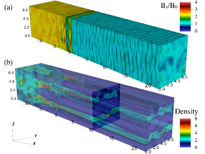
Figure 1: 3D structure of magnetic field $B_{z}/B_{0}$ (top) and density (bottom, in units of $n_{0}$) from a simulation with $\gamma_{0}=3$ and $\sigma=6$ at $\omega_{\rm p}t=9,000$. The $x$ coordinate is measured with respect to the shock location $x_{\rm sh}$, in units of $c/\omega_{\mathrm{p}}$. The upstream is at $x-x_{\rm sh}>0$ and the downstream at $x-x_{\rm sh}<0$. In the bottom panel, the slice at $x-x_{\rm sh}=10\,c/\omega_{\mathrm{p}}$ emphasizes the upstream density structures.

The Poynting flux carried by X-mode and O-mode waves is quantified in Fig. 2(a), via the temporal evolution of $\xi_{\rm X}=\langle(B_{z}-B_{0})^{2}\rangle/B_{0}^{2}$ and $\xi_{\rm O}=\langle B_{y}^{2}\rangle/B_{0}^{2}$ for different magnetizations. The spatial average is taken from $5$ to 30 $c/\omega_{\mathrm{p}}$ ahead of the shock. At late times, the Poynting fluxes settle to a steady state, and we measure their values for shocks with different $\sigma$. At $\sigma\gg 1$, the X-mode power asymptotes to $\xi_{\rm X}\simeq 10^{-2}$, in agreement with earlier 1D and 2D results [22, 23]. In contrast, the O-mode power drops with $\sigma$, approximately as $\xi_{\rm O}\simeq 4\times 10^{-3}\,\sigma^{-1}$.

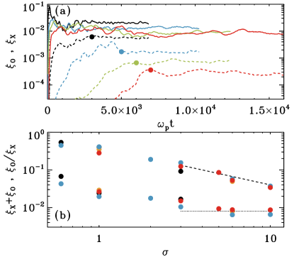
Figure 2: (a) Temporal evolution of the Poynting flux carried by X-modes (solid; $\xi_{\rm X}=\langle(B_{z}-B_{0})^{2}\rangle/B_{0}^{2}$) and O-modes (dashed; $\xi_{\rm O}=\langle B_{y}^{2}\rangle/B_{0}^{2}$), for shocks with $\gamma_{0}=3$ and different magnetizations: $\sigma=1$ (black), 3 (blue), 5 (green), and 10 (red). The filled circles on the dashed lines mark the time when the corresponding shock approaches a quasi-steady state. (b) Steady-state ratio of the O-mode and X-mode powers $\xi_{\rm O}/\xi_{\rm X}$ (upper series of points) and total Poynting flux $\xi_{\rm X}+\xi_{\rm O}$ (lower series of points), as a function of magnetization. Colors indicate different choices of the upstream Lorentz factor $\gamma_{0}=3$ (yellow) or 10 (black), and different domain sizes $L=3.6c/\omega_{\rm p}$ (red and blue) or $7.2c/\omega_{\rm p}$ (yellow and black). The dashed black line indicates $\xi_{\rm O}/\xi_{\rm X}\simeq 0.4\,\sigma^{-1}$, while the dotted black line represents $\xi_{\rm X}+\xi_{\rm O}\simeq 8\times 10^{-3}$.

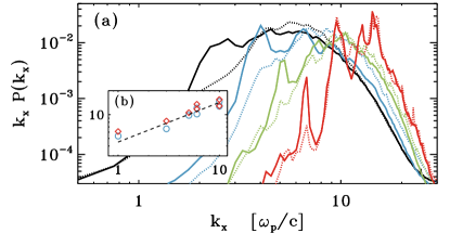
Figure 3: 1D power spectrum $k_{x}P(k_{x})$, where $P(k_{x})=\int P_{\rm 3D}(k_{x},k_{y},k_{z})\,dk_{y}\,dk_{z}$ and $P_{\rm 3D}$ is the 3D power spectrum. Both X-mode (solid) and O-mode (dotted) spectra are normalized so that $\int P(k_{x})dk_{x}=\xi_{\rm X}$, i.e., the O-mode spectrum is shifted up by a factor $\xi_{\rm X}/\xi_{\rm O}$ to facilitate comparison with the X-mode spectrum. Color coding is the same as in Fig. 2(a). The inset shows the energy-carrying wavenumber $\langle k_{x}\rangle=\int k_{x}P(k_{x})dk_{x}/\int P(k_{x})dk_{x}$, in units of $\omega_{\mathrm{p}}/c$, as a function of magnetization (blue for X-mode, red for O-mode). For $\sigma=6$ and 10, the inset also shows results from simulations with higher spatial resolution, $c/\omega_{\mathrm{p}}=50$ cells, yielding similar findings. The dashed black line indicates the scaling $\langle k_{x}\rangle\simeq 4\sqrt{\sigma}\omega_{\mathrm{p}}/c$.

The resulting O/X mode ratio is $\xi_{\rm O}/\xi_{\rm X}\simeq 0.4\,\sigma^{-1}$ for high magnetizations (Fig. 2(b)). This scaling is robust to varying the flow Lorentz factor ($\gamma_{0}=3$ or $10$) and domain size ($L=3.6c/\omega_{\mathrm{p}}$ or $7.2c/\omega_{\rm p}$). The O-mode suppression with increasing $\sigma$ is consistent with previous results of 2D in-plane simulations with $\sigma\lesssim 1$ [20].

The efficiency of the maser emission $f_{\xi}$ is defined in the downstream frame as the fraction of incoming flow energy (electromagnetic + kinetic) converted to precursor wave energy, and we find

$$f_{\xi}=(\xi_{\rm X}+\xi_{\rm O})\left(\frac{\sigma}{1+\sigma}\right)\left(\frac{1-\beta_{\rm sh}}{\beta_{0}+\beta_{\rm sh}}\right)$$ (1)

where $\beta_{\rm sh}$ is the shock speed in units of $c$. While the ratio $\xi_{\rm O}/\xi_{\rm X}$ monotonically drops with $\sigma$, the overall wave energy flux asymptotes to a constant value $\xi_{\rm X}+\xi_{\rm O}\sim\xi_{\rm X}\simeq 0.01$ for $\sigma\gg 1$, and gives $f_{\xi}\simeq 10^{-3}\,\sigma^{-1}$. In the shock maser scenario for FRBs, this quantifies the fraction of the blast wave energy that is converted into FRB energy. The quantity $\xi_{\rm X}+\xi_{\rm O}$ also determines the dimensionless strength parameter of precursor waves at $\sigma\gg 1$: $a\sim 0.3\gamma_{0}\sqrt{\xi_{\rm X}+\xi_{\rm O}}\simeq 0.03\,\gamma_{0}$ [22]. For ultra-relativistic shocks the strength parameter can exceed unity.

The spectrum of precursor waves is presented in Fig. 3 for different magnetizations. The spectra are computed in the post-shock frame, from the same upstream region ($5\,c/\omega_{\mathrm{p}}<x-x_{\rm sh}<30\,c/\omega_{\mathrm{p}}$) where we extracted the precursor efficiency. Both X-mode and O-mode spectra peak at higher wavenumbers for larger magnetizations. This is also illustrated by the dependence on $\sigma$ of the energy-carrying wavenumber $\langle k_{x}\rangle\simeq 4\sqrt{\sigma}\omega_{\mathrm{p}}/c$ (inset in Fig. 3(b)). Fig. 3 demonstrates that at high wavenumbers ($k_{x}/\langle k_{x}\rangle\gtrsim 1$) X-mode and O-mode spectra are similar. They differ, however, at lower wavenumbers; the spectral feature at $k_{x}\simeq 0.5\langle k_{x}\rangle$ only appears in the X-mode. Near this wavenumber, the O/X mode ratio is one order of magnitude below the average $\xi_{\rm O}/\xi_{\rm X}$.

X-Mode Emission Mechanism.— The X-mode generation is well captured in 1D models. One example with $\gamma_{0}=10$ and $\sigma=3$ is shown in Fig. 4. The X-mode waves appear as ripples in $B_{z}$ propagating into the upstream region, after the width of the shock cavity has settled into a steady state ($\omega_{\rm p}t\gtrsim 1350$). The current near the leading soliton then remains nearly time-independent. The oscillating current $J_{y}$ emitting the X-mode waves is localized downstream of the second soliton, at $-10\,c/\omega_{\mathrm{p}}\lesssim x-x_{\rm sh}\lesssim-5\,c/\omega_{\mathrm{p}}$ (Fig. 4(b)). The generated waves propagate both toward the downstream (where they are eventually absorbed) and through the density cavity into the upstream.

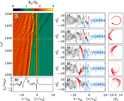
Figure 4: Shock “breathing,” as observed in the simpler 1D simulation ($\gamma_{0}=10$, $\sigma=3$), which fully captures the X-mode generation. (a) Spatio-temporal structure of $B_{z}/B_{0}$. (b) Electric current density $J_{y}/en_{0}c$ at $\omega_{\rm p}t=1400$ (the moment indicated by the upper dashed line in panel (a)). (c)-(g) Sequence of five snapshots for randomly sampled positrons in the $x-\gamma\beta_{y}$ phase space and for a selected subset of positrons (in red) in the $\gamma\beta_{x}-\gamma\beta_{y}$ momentum space. The snapshots cover the time interval $1393<\omega_{\rm p}t<1400$ (indicated by the two horizontal dashed lines in (a)). Positrons highlighted in red are selected so that at $\omega_{\rm p}t=1400$ they contribute to the current peak at $-10\,c/\omega_{\mathrm{p}}\lesssim x-x_{\rm sh}\lesssim-5\,c/\omega_{\mathrm{p}}$ in (b). The blue lines show $(E^{2}-B^{2})/(E^{2}+B^{2})$ (for these curves, the vertical boundaries correspond to -1 and 1).

In the shock frame, which moves with Lorentz factor $\approx\sqrt{\sigma}$ relative to the downstream, the field satisfies the jump condition $B_{d,\rm sh}/B_{u,\rm sh}=1+1/2\sigma$ [29]. Here, $B_{u,\rm sh}\simeq 2\sqrt{\sigma}B_{0}$ and $B_{d,\rm sh}$ are the upstream and downstream fields, respectively. The net surface current of the multiple soliton structure of the shock is $\Sigma\sim c(B_{d,\rm sh}-B_{u,\rm sh})/4\pi\sim cB_{0}/(4\pi\sqrt{\sigma})$. Assume that the surface current varies with some amplitude $\zeta=\delta\Sigma/\Sigma$. In the shock frame, the emitted wave has the amplitude $\delta B_{\rm sh}\sim\zeta B_{0}/(2\sqrt{\sigma})$. This wave, viewed in the downstream frame of the simulation, has $\delta B\approx\sqrt{\sigma}\,\delta B_{\rm sh}$, which gives the precursor with amplitude $\sim\zeta B_{0}$ and $\xi_{\rm X}\approx\zeta^{2}$. Thus, the constant $\xi_{\rm X}\approx 10^{-2}$ observed at $\sigma\gg 1$ is consistent with the constant amplitude $\zeta\approx 0.1$ of the shock fluctuations.

Most positrons in the wave emission region ($-10\,c/\omega_{\mathrm{p}}<x-x_{\rm sh}<-5\,c/\omega_{\mathrm{p}}$) have $\gamma\beta_{y}>0$. By symmetry of the 1D simulation, at any given location electrons and positrons have the same densities and $\gamma\beta_{x}$, and opposite $\gamma\beta_{y}$, which determines the current $J_{y}$. Fig. 4 shows the history of the positrons ending up at $-10\,c/\omega_{\mathrm{p}}\lesssim x-x_{\rm sh}\lesssim-5\,c/\omega_{\mathrm{p}}$. At the shock, they initially form a ring in momentum space [17]. Their subsequent motion through the density cavity is affected by the waves generated by earlier generations of shocked particles. The waves create (by linear superposition) regions of $E>B$ (see the blue lines in Fig. 4). The $E>B$ region extends across roughly half a wavelength.

Particles exposed to $E>B$ get accelerated, at a rate that depends on the wave amplitude and the particle $\beta_{y}$. This wave-particle interaction increases the energy spread of incoming particles, so their arc in the $\gamma\beta_{x}-\gamma\beta_{y}$ space grows in radius and thickness, as they move past the leading soliton (compare Fig. 4(d) and (c)). The particles at the inner edge of the arc (lower $\gamma$) gyrate faster than the particles at the outer edge (higher $\gamma$). Initially, lower-energy positrons lag in phase behind higher-energy ones (Fig. 4(e); positrons move clockwise in the $\gamma\beta_{x}-\gamma\beta_{y}$ plane), but later catch up due to their shorter gyroperiod. This creates gyro-phase bunching (Fig. 4(f) and (g)), and produces an intermittent enhancement of current density $J_{y}$. The current oscillates on the gyroperiod of post-shock particles and its harmonics, generating the X-mode.

Without wave activity, the magnetic field in the cavity is $\boldsymbol{B}_{0}$. The condition $E>B$ is realized where the wave has $\delta B_{z}<0$ and $\delta E_{y}<0$, so $|B_{z}|=|B_{0}+\delta B_{z}|<B_{0}$ and $|E_{y}|=|-E_{0}+\delta E_{y}|>E_{0}$. Since $E_{y}<0$, positrons are accelerated in $E>B$ regions if their $\beta_{y}<0$ (conversely, $\beta_{y}>0$ for electrons). This condition occurs in half of the cavity, just behind the leading soliton. Therefore, the process of wave generation is self-reinforced if the half-wavelength of the X-mode is approximately equal to the half-thickness of the cavity. This explains why the peak frequency of the wave spectrum corresponds to an eigenmode of the cavity [22].

Thus, X-mode waves are generated by a non-local positive feedback loop: (i) in the density cavity, waves propagating upstream lead to $E>B$, which perturbs the energies of fresh particles entering the cavity from the shock front; (ii) higher-energy particles gyrate slower than lower-energy ones, leading to gyro-phase bunching; (iii) this produces a net current oscillating on the particle gyration time, leading to more wave production. The non-locality of the feedback loop differentiates our mechanism from the standard (local) description of the synchrotron maser. Also, the precursor emission in high-$\sigma$ shocks cannot be attributed to the standard maser mechanism, since a seed wave cannot be considerably amplified while particles cross the shock [4].

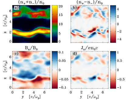
Figure 5: Charge separation and field line bending (from the 3D simulation presented in Fig. 1), explaining the O-mode generation. At the location of the leading soliton $x=x_{\rm sh}$, we show 2D $y-z$ slices of: (a) $n_{+}+n_{-}$, where $n_{+}$ and $n_{-}$ are the positron and electron number densities; (b) $n_{+}-n_{-}$, as a proxy for charge separation; (c) $B_{x}/B_{0}$; (d) current density $J_{z}/en_{0}c$.

O-Mode Emission Mechanism.— The physics of the O-mode generation is inherently 3D. In Fig. 5, we employ the same 3D simulation of Fig. 1, and show 2D slices at the location of the leading soliton, $x=x_{\rm sh}$ .

The O-mode-generating current $J_{z}$ is ultimately related to the sheet-like density layers produced by self-focusing of the precursor waves (Fig. 5(a)). Significant charge separation develops at the boundaries of the density sheets (Fig. 5(b)), because positrons and electrons flowing into the shock gyrate in opposite directions. This leads to charge separation as long as the sheets are not invariant along the $y$ direction perpendicular to the initial field, e.g., for tilted or inhomogeneous sheets.

If only the $B_{z}$ component was present, the charge bunches would move in the $x-y$ plane, and would not generate any $J_{z}$. A nonzero $B_{x}$ appears at the shock because the non-uniform ram pressure of the sheets causes field-line bending in the $x$-$z$ plane. Its energy density scales with the incoming kinetic energy density, $B_{x}^{2}/B_{0}^{2}\propto\gamma_{0}n_{0}mc^{2}/B_{0}^{2}\propto\sigma^{-1}$. Thus, the field lines near the front are no longer perpendicular to the flow velocity, and the charge bunches slide along the field, developing a small $\beta_{z}\simeq\beta_{\parallel}\simeq\sqrt{B_{x}^{2}/B_{0}^{2}}$, which in turn leads to the O-mode-generating $J_{z}$ (Fig. 5(d)). This implies that the O/X mode power ratio should scale as $\xi_{\rm O}/\xi_{\rm X}\propto\beta_{z}^{2}\propto B_{x}^{2}/B_{0}^{2}\propto\sigma^{-1}$, as observed in Fig. 2(b).

In summary, O-mode generation can be properly captured only in 3D. It requires breaking the symmetry both (i) along $y$ — enabling charge separation at the boundaries of the density sheets when the incoming particles begin to gyrate in the shock-compressed field; and (ii) along $z$ ($\boldsymbol{B}_{0}$ direction) — enabling $B_{x}$ generation via field-line bending by the high-density sheets colliding with the shock. The charge bunches slide along the perturbed field lines, creating the variable O-mode current $J_{z}$.

Summary.— By means of 3D PIC simulations, we have characterized O-mode and X-mode waves emitted by relativistic magnetized shocks propagating in magnetically-dominated ($\sigma>1$) pair plasmas. The fraction of incoming energy converted into precursor waves is $f_{\xi}\simeq 10^{-3}\,\sigma^{-1}$, and the energy-carrying wavenumber is $\langle k_{x}\rangle\simeq 4\,\omega_{\rm c}/c$. The O/X mode power ratio is $\xi_{\rm O}/\xi_{\rm X}\simeq 0.4\,\sigma^{-1}$, regardless of the shock Lorentz factor. While O-mode and X-mode spectra overlap at high wavenumbers, the narrow spectral feature at $k_{x}\simeq 0.5\langle k_{x}\rangle$ is much stronger in the X-mode.

Our results provide important plasma-physical inputs for FRB emission models, by demonstrating that high-$\sigma$ shocks can emit electromagnetic waves with a high degree of linear polarization, as observed in some FRBs [15]. By calculating the power-weighted Stokes’ parameters for a line of sight along the shock normal, one can compute the degree of linear polarization $P=Q/I$ [31, $U=V=0$ is well satisfied in our simulations] intrinsic to the shock emission . Since $Q=\xi_{\rm X}-\xi_{\rm O}$ and $I=\xi_{\rm X}+\xi_{\rm O}$, the degree of linear polarization for $\xi_{\rm O}/\xi_{\rm X}\ll 1$ is $P\simeq 1-2\xi_{\rm O}/\xi_{\rm X}\simeq 1-0.8\sigma^{-1}$.

xx

I Supplementary Material: Numerical Simulation Parameters

The plasma skin depth in our 3D simulations is well resolved with $c/\omega_{\mathrm{p}}=25$ cells, to capture the high-frequency wave spectrum and mitigate the numerical Cerenkov instability [19]. For $\sigma=6$ and $10$, we also present results with doubled resolution, $c/\omega_{\mathrm{p}}=50$ cells. As shown in the main text, the energy-carrying wavenumber of the wave spectrum is $\simeq 4\,\sqrt{\sigma}\,\omega_{\rm p}/c$, so a careful assessment of convergence with respect to spatial resolution is particularly important at high magnetizations. We vary the transverse box size $L$ between 3.6 and $7.2\,c/\omega_{\mathrm{p}}$, which we find sufficient to capture multi-dimensional effects. We employ periodic boundary conditions in $y$ and $z$. The upstream plasma has 3 particles per cell per species, but we have tested that even 1 particle per cell gives converged results. The numerical speed of light is $0.45\,{\rm cells/timestep}$. Our longest simulations extend up to $\sim 16,000\,\omega_{\mathrm{p}}^{-1}$ ($\sim 900,000$ timesteps).

The simulations are optimized in $x$ to enable longer numerical experiments. The incoming plasma is injected by a “moving injector,” which moves along $+{\hat{x}}$ at the speed of light, thus retaining all regions in causal contact with the shock. The box is expanded in $x$ as the injector approaches the right boundary [18]. The left edge of the downstream region (hereafter, the “wall”) acts as a particle reflector and provides conducting boundary conditions for the electromagnetic fields. It is initially located at $x=0$, but gets periodically relocated closer to the shock to save memory and computational time; we ensure a minimum distance of $\sim 100\,c/\omega_{\mathrm{p}}$ between the wall and the shock. We also performed simulations with a stationary wall and verified that the wall relocation does not influence the shock or the precursor waves [23].

We also present one 1D simulation with $\gamma_{0}=10$ and $\sigma=3$ to clarify the physics of X-mode emission. The 1D run resolves the skin depth with 50 cells and is initialized with 40 particles per cell.

References

- Petroff et al. [2019] E. Petroff, J. W. T. Hessels, and D. R. Lorimer, A&A Rev. 27, 4 (2019), eprint 1904.07947.
- Cordes and Chatterjee [2019] J. M. Cordes and S. Chatterjee, ARA&A 57, 417 (2019), eprint 1906.05878.
- Platts et al. [2019] E. Platts, A. Weltman, A. Walters, S. P. Tendulkar, J. E. B. Gordin, and S. Kandhai, Phys. Rep. 821, 1 (2019), eprint 1810.05836.
- Lyubarsky [2021] Y. Lyubarsky, Universe 7, 56 (2021), eprint 2103.00470.
- Katz [2016] J. I. Katz, Modern Physics Letters A 31, 1630013 (2016), eprint 1604.01799.
- Scholz and Chime/Frb Collaboration [2020] P. Scholz and Chime/Frb Collaboration, The Astronomer’s Telegram 13681, 1 (2020).
- Bochenek et al. [2020] C. D. Bochenek, V. Ravi, K. V. Belov, G. Hallinan, J. Kocz, S. R. Kulkarni, and D. L. McKenna, Nature (London) 587, 59 (2020), eprint 2005.10828.
- Beloborodov [2017] A. M. Beloborodov, ApJ 843, L26 (2017), eprint 1702.08644.
- Metzger et al. [2019] B. D. Metzger, B. Margalit, and L. Sironi, MNRAS 485, 4091 (2019), eprint 1902.01866.
- Beloborodov [2020] A. M. Beloborodov, Astrophys. J. 896, 142 (2020), eprint 1908.07743.
- Yuan et al. [2020] Y. Yuan, A. M. Beloborodov, A. Y. Chen, and Y. Levin, ApJ 900, L21 (2020), eprint 2006.04649.
- Alsop and Arons [1988] D. Alsop and J. Arons, Physics of Fluids 31, 839 (1988).
- Hoshino and Arons [1991] M. Hoshino and J. Arons, Physics of Fluids B 3, 818 (1991).
- Note [1] Note1, the generation of coherent emission is not directly due to wave amplification via a maser process, but still we shall refer to this as the “synchrotron maser,” because this term is widely used in the literature.
- Michilli et al. [2018] D. Michilli, A. Seymour, J. W. T. Hessels, L. G. Spitler, V. Gajjar, A. M. Archibald, G. C. Bower, S. Chatterjee, J. M. Cordes, K. Gourdji, et al., Nature (London) 553, 182 (2018), eprint 1801.03965.
- Langdon et al. [1988] A. B. Langdon, J. Arons, and C. E. Max, Physical Review Letters 61, 779 (1988).
- Gallant et al. [1992] Y. A. Gallant, M. Hoshino, A. B. Langdon, J. Arons, and C. E. Max, Astrophys. J. 391, 73 (1992).
- Sironi and Spitkovsky [2009] L. Sironi and A. Spitkovsky, Astrophys. J. 698, 1523 (2009), eprint 0901.2578.
- Iwamoto et al. [2017] M. Iwamoto, T. Amano, M. Hoshino, and Y. Matsumoto, Astrophys. J. 840, 52 (2017), eprint 1704.04411.
- Iwamoto et al. [2018] M. Iwamoto, T. Amano, M. Hoshino, and Y. Matsumoto, Astrophys. J. 858, 93 (2018), eprint 1803.10027.
- Plotnikov et al. [2018] I. Plotnikov, A. Grassi, and M. Grech, MNRAS 477, 5238 (2018), eprint 1712.02883.
- Plotnikov and Sironi [2019] I. Plotnikov and L. Sironi, MNRAS 485, 3816 (2019), eprint 1901.01029.
- Babul and Sironi [2020] A.-N. Babul and L. Sironi, MNRAS 499, 2884 (2020), eprint 2006.03081.
- Spitkovsky [2005] A. Spitkovsky, in Astrophysical Sources of High Energy Particles and Radiation, edited by T. Bulik, B. Rudak, & G. Madejski (2005), vol. 801 of AIP Conf. Ser., p. 345, eprint arXiv:astro-ph/0603211.
- Hoshino [2001] M. Hoshino, Progress of Theoretical Physics Supplement 143, 149 (2001).
- Drake et al. [1974] J. F. Drake, P. K. Kaw, Y. C. Lee, G. Schmid, C. S. Liu, and M. N. Rosenbluth, Physics of Fluids 17, 778 (1974).
- Sobacchi et al. [2021] E. Sobacchi, Y. Lyubarsky, A. M. Beloborodov, and L. Sironi, MNRAS 500, 272 (2021), eprint 2010.08282.
- Note [2] Note2, we remark, however, that in Iwamoto et al. [20] the O-mode emission was attributed to gyro-phase bunching in Weibel-generated fields, which cannot operate in the high- shocks presented in this Letter.
- Pétri and Lyubarsky [2007] J. Pétri and Y. Lyubarsky, A&A 473, 683 (2007), eprint 0707.1782.
- Note [3] Note3, even though we focus on the leading soliton, the features described below are observed throughout the density cavity until the second soliton.
- Rybicki and Lightman [1979] G. B. Rybicki and A. D. Lightman, Radiative Processes in Astrophysics (John Wiley & Sons, Inc., 1979).
- Note [4] Note4, detailed calculations of the observed polarization degree from FRB-producing shocks, accounting for both shock curvature and propagation effects, will be presented elsewhere.