Visual Relationship Forecasting in Videos

Abstract

Real-world scenarios often require the anticipation of object interactions in unknown future, which would assist the decision-making process of both humans and agents. To meet this challenge, we present a new task named Visual Relationship Forecasting (VRF) in videos to explore the prediction of visual relationships in a reasoning manner. Specifically, given a $\textless$subject-object$\textgreater$ pair with $H$ existing frames, VRF aims to predict their future interactions for the next $T$ frames without visual evidence. To evaluate the VRF task, we introduce two video datasets named VRF-AG and VRF-VidOR, with a series of spatio-temporally localized visual relation annotations in a video. These two datasets densely annotate 13 and 35 visual relationships in 1923 and 13447 video clips, respectively. In addition, we present a novel Graph Convolutional Transformer (GCT) framework, which captures both object-level and frame-level dependencies by spatio-temporal Graph Convolution Network and Transformer. Experimental results on both VRF-AG and VRF-VidOR datasets demonstrate that GCT outperforms the state-of-the-art sequence modelling methods on visual relationship forecasting.

1 Introduction

Visual relationships among objects play important roles in many video understanding tasks, such as video captioning, action recognition and video visual question answering. In such tasks, visual relatiion triplets, shown as $\textless$subject-predicate-object$\textgreater$, or visual scene graphs are considered as the effective decriptions of visual scene. Based on these representations, video visual relationship research aims to detect visual relationship triplets or construct dynamic visual scene graph for the videos.

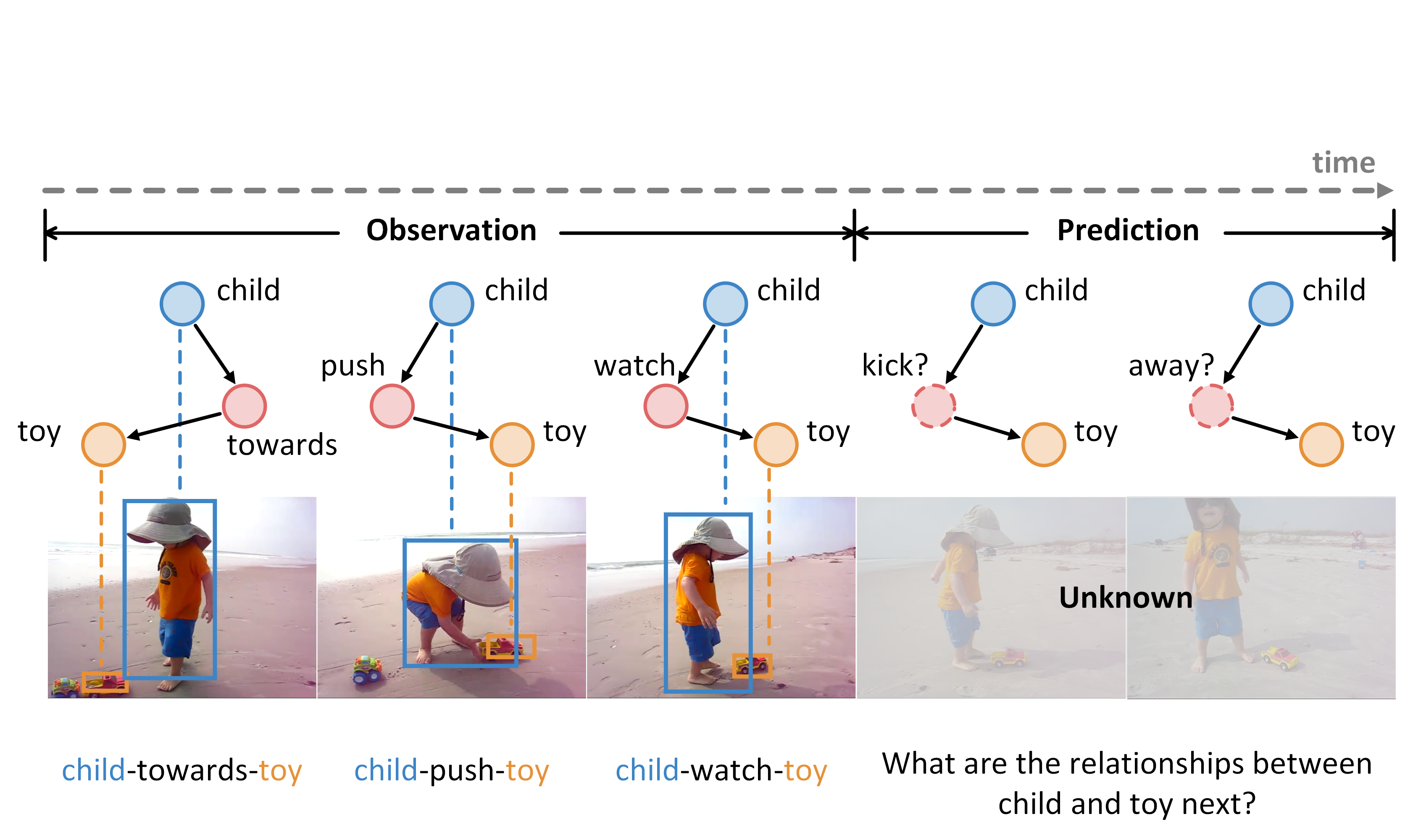
Figure 1: The illustration of the proposed Visual Relationship Forecasting in Videos (VRF) task. Given a history of $H$ previous frames and a specific subject-object pair, VRF aims to predict their future relationships for the next $T$ frames without observation.

Current efforts in visual relationship research are mainly based on the fully-observation of visual evidence. In other words, these tasks focused more on detecting the object interactions based on observation rather than reasoning about the spatio-temporal connections among predicates. However, in the real-world scenarios, the ability of predicting possible interactions between objects in future is regarded as one of the fundamental challenges in video understanding. For exmaple, the next possible triplet after $\textless$person-hold-apple$\textgreater$ may be $\textless$person-throw-apple$\textgreater$ or $\textless$person-eat-apple$\textgreater$. Anticipating the possible predicates can provide a reasonable description on visual scenes in the near feature, which can assist the tasks like video prediction, video question answering and trajectory prediction. Furthermore, the ability of predicting object interactions without visual evidence can also support the decision-marking process of both humans and agents.

To explore this open challenges, we introduce a new video reasoning task named Visual Relationship Forecasting (VRF) in videos. With the limited observation of visual evidence, VRF aims to anticipate future interactions between a definited $\textless$subject-object$\textgreater$ pair. For the example in Figure 1, given a pair of $\textless$subject-object$\textgreater$ ($\textless$child-toy$\textgreater$) and a sequence of previous relationship triplets ($\textless$child-watch-toy$\textgreater$, $\textless$child-touch-toy$\textgreater$, $\textless$child-grab-toy$\textgreater$), our goal is to predict several future triplets ($\textless$child-hold-toy$\textgreater$, $\textless$child-release-toy$\textgreater$) without visual evidence. Compared to the tasks that are based on fully observation, VRF emphasizes reasoning and anticipating future relationships through limited visual scenarios.

To benchmark the proposed VRF task, we reorganize the annotations based on the existing video datasets and introduce two datasets named VRF-AG and VRF-VidOR. These two datasets densely annotate 13 and 35 visual relationships in 1923 and 13447 video clips, respectively. For each video, there are a series of spatio-temporally localized visual relation triplet annotations for a specific $\textless$subject-object$\textgreater$ pair. In addition, we present a novel baseline method named Graph Convolutional Transformer (GCT) for the VRF task as current methods in visual relationship detection are not specialized for visaul relationship forecasting. For example, most of the exsiting models were designed based on visual observation which is not provided by VRF settings. Moreover, current methods often detect several $\textless$subject-object$\textgreater$ pairs in a video while the VRF only focuses one pair in each video. GCT represents the sptio-temporal dependencies among relation triplets to predict the possible relation triplets in the future. Spatio-Temporal Graph Convolution Network (ST-GCN) is introduced to model the object-level interactions while Transformer is utilized to capture the frame-level interactions. Experimental results on both VRF-AG and VRF-VidOR datasets demonstrate that GCT outperforms the state-of-the-art time series modeling methods on visual relationship forecasting.

The contribution of the paper can be summarized as:

• To reason about the sptio-temporal dependencies of visual relationship, we present a new task named Visual Relationship Forecasting in videos (VRF). For a given video and a specific $\textless$subject-object$\textgreater$ pair, VRF aims to anticipate the future interactions between the subject and object with limited observation.

• To evaluate the prposed VRF task, two benchmark datasets with spatio-temporally localized visual relation triplet annotations are established in this paper for further study and discussion in visual relationship reasoning in videos.

• A novel framework named Graph Convolutional Transformer (GCT) is proposed to benchmark the task. In GCT, Spatio-Temporal Graph Convolution Network (ST-GCN) is introduced to model the object-level interactions while Transformer is utilized to capture the frame-level interactions.

2 Background and Preliminaries

2.1 Visual Relationship Detection in Videos

Visual Relationship Detection (VRD) in videos aims to detect several relation triplets in a visual scene based on fully visual observation. Different from visual relationship detection in static image [1, 2, 3, 4, 5, 6, 7] that focuses on detection object relationships based on a moment of observation, video visual relationship detection [8] requires addtional spatial-temporal modeling among time series. To address the spatio-temporal modeling challenge, Tsai et al. [9] constructed a Conditional Random Field (CRF) on a fully-connected spatio-temporal graph to exploit the statistical dependency between relational entities. Qian et al. [10] abstracted videos into fully-connected spatial-temporal graphs. However, current detection methods are built on fully observation of the video, which is not suitable for relationship forecasting. Moreover, the existing methods in video VRD often divided the task into object tracking stage and relationship detection stage. The relationship detection performance is overly dependent on the object detection results, which ignoreed to emphasize the importance of visual relationship reasoning. To strengthen reasoning ability and spatio-temporal modeling ability, we introduce a new task for visual relationship reasoning named VRF. Compared with VRD, this task simplifies object detection process and focuses more on capturing the logical associations and inner interactions for specific subject-object pair among time.

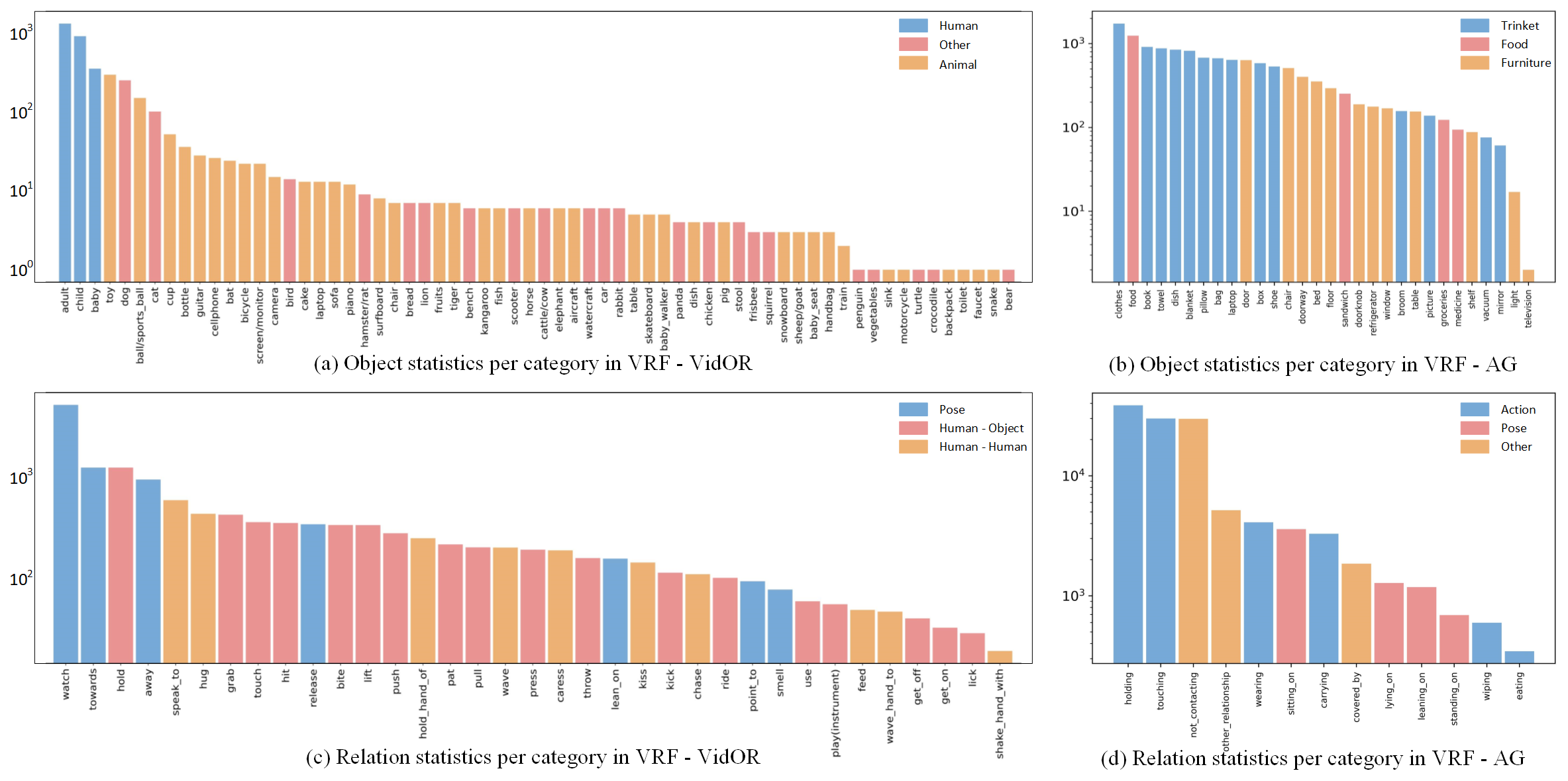
Figure 2: Object and relation statistics per category with colors indicating different types in VRF-VidOR and VRF-AG datasets.

Table 1: Comparison of VRF-VidOR Dataset and VRF-AG Dataset on Dataset Statistics.

	Video	Predicate	Object	Generation Method of Testing Set
VRF-VidOR	1723	35	64	Random Sampling
VRF-AG	13447	13	30	Category Average Sampling

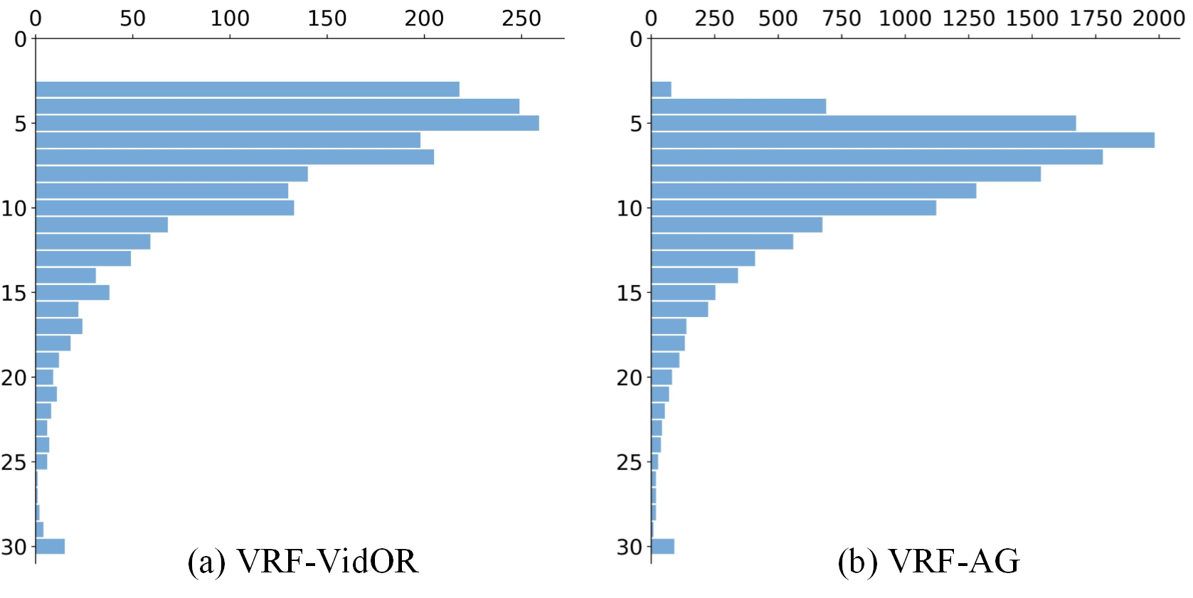
Figure 3: The number of key frames per video in VRF-VidOR and VRF-AG datasets.

2.2 Future Prediction

Future prediction in video can be roughly divided in to two themes: 1) generating future frames [11, 12, 13, 14, 15, 16, 17, 18] and 2) predicting future labels or states [19, 20, 21, 22, 23, 24, 25, 26, 27, 28]. In the first theme, generative models are required to predict future frames from intermediate representations. For the second theme, a wide variety of future state are involved, from low-level trajectories to high-level semantic outputs. The proposed VRF task is based on the aforementioned future prediction tasks and can be classified into the second theme. Compared to the exsiting feature prediction task, the characteristics of VRF can be summarized as the following two points. Firstly, VRF performs forecasting on the unknown future frames, which demands deeply understanding of historical observation and reasoning based on priors. Secondly, different from the task that has multiple agents, VRF focuses on the relationship forecasting among a specific pair of $\textless$subject-object$\textgreater$.

2.3 Visual Reasoning in Videos

Visual reasoning has attracted growing interests recently [29, 30, 31, 32, 33]. Spatial and temporal dependencies are incorporated to understand the video context with sequence modeling methods or graph structures. For temporal relation reasoning, Temporal Relation Network (TRN) [34] was designed to learn and reason about temporal dependencies between video frames at multiple time scales. Rohit et al. [35] proposed a video action transformer network to capture the temporal dependencies in videos for action recognition. In addition, Graph structure serves as a significant tool to reason about spatio-temporal data or non-structural data [36, 37, 38, 39]. Object Relation Network (ORN) [40] is a module for performing spatio-temporal reasoning between detected object instances in the video. It is able to capture object moves, arrivals and interactions. In this paper, VRF aims to predict relationship in future with a reasoning manner, which requires the fully exploration about the information in the past and the anticipation of the relationship between a pair of subject and object without observation.

3 Task Definition

Visual Rrelationship Forecasting (VRF) aims to anticipate future interactions between a definited $\textless$subject-object$\textgreater$ pair. More specifically, let $O$ and $P$ denote the object set and predicate set, respectively, then the relationship set $R$ can be defined as $R=\{r(s,p,o)|s,o\in O,p\in P\}$, where $s$, $p$ and $o$ are respectively the subject, predicate and object in a relationship triplet $r(s,p,o)$. VRF aims to compute the probability:$\mathbf{P}(r)=\mathbf{P}\left(p^{0:T}\mid V^{-H:0},s,o\in O\right)$, where $V^{t}$ is the frame at time $t$, $t=0$ represents the present. $V^{-H:0}$ denotes the visual history of $H$ previous key frames. $p^{0:T}$ represents the predicates in the future $T$ key frames.

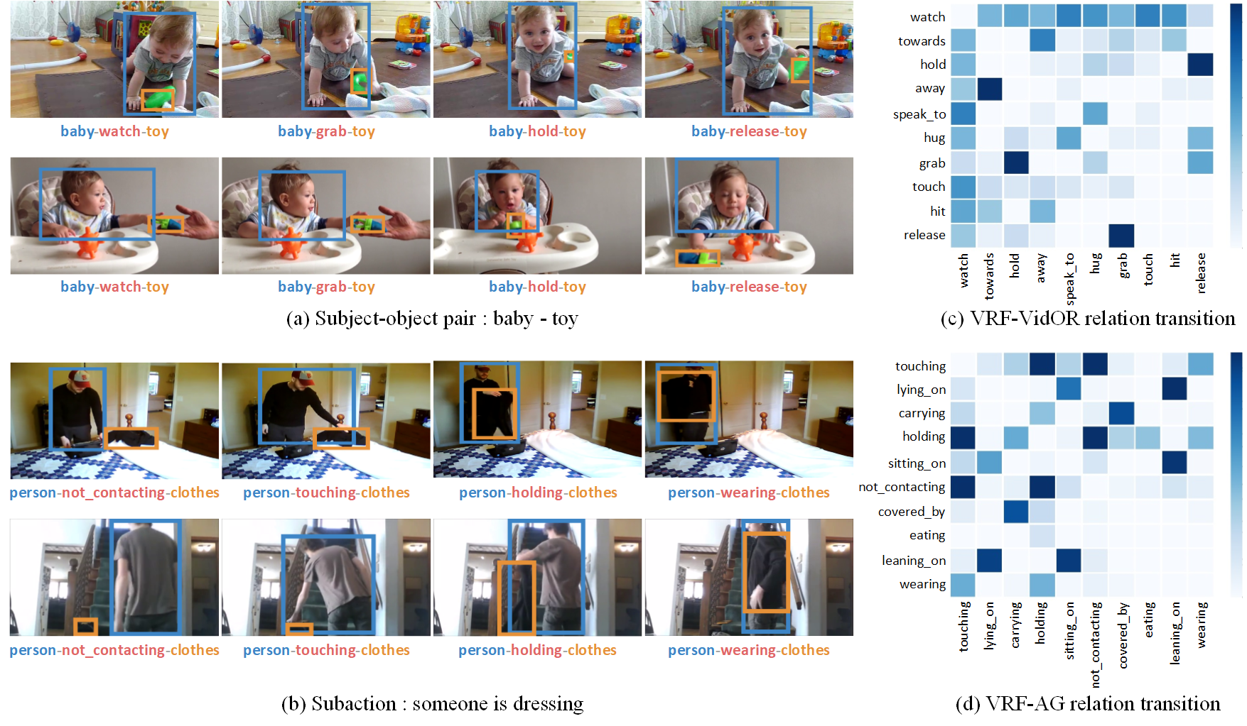
Figure 4: Examples and statistical distribution of relation transition in VRF-VidOR and VRF-AG datasets. We show examples of how relationship transfer within same subject-object pair (a) in VRF-VidOR dataset and same action category (b) in VRF-AG dataset.

4 Dataset

In this paper, two video datasets, i.e. VRF-AG and VRF-VidOR are established from Action Genome dataset [41] and video visual relationship detection dataset [8], respectively.

4.1 Dataset Generation

In this section, we briefly introduce the generation process including the principles of building the relation vocabulary, the selection of the candidate videos and key frames and the cleanning-up process.

Predicate Vocabulary Generation. We follow three rules to generate the predicate vocabulary: semantics, visuality and quantity. 1) Semantics Rule. In current VRD datasets, there are a lot of spatial predicates (e.g., above, beneath) which provides limited information for video scene understanding. In order to reduce the interference of spatial annotations on reasoning, we only collect data with semantic relation annotations. 2) Visuality Rule. The predicate categories in the dataset vocabulary must have clear visual signatures, so some categories that cannot be accurately judged from visual information are filtered out (e.g., shout_at). 3) Quantity Rule. To reduce the influence of long-tail distribution in the original datasets, predicate categorie annotations that account for less than 1% of the total are deleted (e.g., twisting, squeeze).

Figure 5: Object-Relation Interaction. The left side of the figure represents the relationship categories in the data set, and the right side of the figure represents the object categories in the dataset.

Video and Key Frames Selection. The constant change of the predicate is regarded as a prerequisite for reasoning in VRF. Therefore, we select the data containing more than three kinds of predicate annotations for a specific $\textless$subject-object$\textgreater$ pair in the video. Moreover, if multiple predicates are repeated consecutively, we select two key frames in the interval of their occurrence.

Cleaning and Denoising. Excessively long timing video clips will cause great difficulty in visual relationship forecasting. By screening the length of video clips, videos with a total number of key frames greater than 30 are truncated. On the other hand, we try to filter videos and annotations to balance the number of predicate categories in the dataset which would alleviate the impact of the biased data distribution.

4.2 Dataset Statistics

Object Categories. Figure 2 (a) and (b) show the log-distribution of object categories in VRF-AG and VRF-VidOR datasets. There are 30 object categories in VRF-AG dataset and 64 object categories in VRF-VidOR dataset, respectively. In VRF-AG dataset, there are 26894 bounding boxes in train/val set. Each video has a person bounding box and an object bounding box. The number of objects in Trinket, Food and Furniture accounts for 65%, 13% and 22% in VRF-AG dataset. In VRF-VidOR dataset, there are 3846 bounding boxes in the train/val set. Each video has a subject bounding box and an object bounding box. The number of objects of Human, Animal and Other accounts for 67%, 12% and 21% in VRF-VidOR dataset. In particular, we can also find that not all subjects are person in VRF-VidOR dataset. Overall, compared with VRF-AG dataset, VRF-VidOR dataset has more object categories, which will increase the data diversity.

Predicate Categories. Figure 2 (c) and (d) show the distribution of relation categories in VRF-AG and VRF-VidOR datasets. There are 13 predicate categories in VRF-AG dataset and 35 predicate categories in VRF-VidOR dataset, respectively. Each video is annotated a pair of $\textless$subject-object$\textgreater$ and a time-series of predicates. The number of predicates of Pose, Human-Object and Human-Human accounts for 55%, 31% and 14% in VRF-VidOR dataset, while the number of predicates in Action, Pose and Other accounts for 64%, 5% and 31% in VRF-AG dataset. Since the predicate number in VRF-VidOR is more than that in VRF-AG, it is more difficult to performming forecasting on the VRF-VidOR dataset.

Video Length. Figure 3 shows the distribution of the number of key frames per video in the proposed two datasets. As it can be seen in figure, the overall distribution is close to a Gaussian distribution. The length of most video is concentrated in 4-12 key frames, and the longest length is 30 key frames. In this paper, we prepare 3 subsets for each dataset, containing 5, 10, and 15 key frames respectively.

Training and Test Sets. For VRF-AG dataset, 50 videos for each relation category with a total of 650 videos are selected for test set and the remaining 12797 videos are used to form the training set. For VRF-VidOR dataset, we randomly select 400 video for test set with at least one sample from each category. The remaining 1523 videos are prepared for training set.

4.3 Dataset Characteristics

Example. Figure 4 (a) and (b) show annotation examples of same subject-object pair $\textless$baby-toy$\textgreater$ and same action someone is dressing, respectively. We can found that for a specific $\textless$baby-toy$\textgreater$ pair or action annotation, the possible predicate sets are similar regardless of different visual appearance. For example, the two $\textless$baby-toy$\textgreater$ examples both have the predicate series of $watch\Rightarrow grab\Rightarrow hold\Rightarrow release$; and the predicates between person and clothes in action someone is dressing follow the series of $not\_contacting\Rightarrow touching\Rightarrow holding\Rightarrow wearing$. These examples indicate some learnable relation transition trends.

Relation Transition. Figure 4 (c) and (d) show statistical distribution of relation transition in two datasets. We calculate the number of all relation transition and normalize them within the same class of relation. In VRF-VidOR dataset, the weights of $grab\Rightarrow hold$ and $hold\Rightarrow release$ are high as we can see in the Figure 4 (a). The relation class of $watch$ may be transferred to many kinds of relation and these may also be transferred to $watch$. In VRF-AG dataset, $not\_contacting$ is mainly transferred to $touching$ and $holding$, and $touching$ is also easy be transferred to $holding$ and $not\_contacting$. The probability of transferring from $holding$ to $wearing$ is also in the top three. All of the above have proved that relation transition has temporal tendency, so we designed the VRF task to learn the regularity of relation transition in videos.

Object-Relation Interacion. Figure 5 shows the object-relation interaction in the VidOR data set. The left side of the figure represents the relationship categories in the data set, and the right side of the figure represents the object categories in the dataset. It can be seen from the figure that the relationship-object interaction of the data set is more complicated, which also indicates that the task of predicting the video visual relationship is difficult. A large number of relationship categories such as holding and touching interact with almost all objects. A small number of relationship categories such as eating also interacts with at least four objects, namely sandwich, medicine, groceries and food. The number of objects is relatively balanced. The more numerous objects include bag, groceries, towel, shoe and so on. Objects with a small number include television, picture and so on.

Figure 6: The framework of the Graph Convolutional Transformer (GCT) can be divided into three parts: spatial modeling, temporal modeling and message passing. For spatial information, we construct a spatial graph for every key frame to model the interaction between the given subject-object pairs. For temporal information, we utilize a transformer to capture more accurate temporal changes of object. In addition, in order to strengthen the connection of spatiotemporal features, we design the spatiotemporal message passing module as the link of spatial and temporal features.

5 Graph Convolutional Transformer

5.1 Framework

To benchmark the VRF task, a reasoning framework named Graph Convolutional Transformer (GCT) is proposed in these paper. GCT can be divided into three parts: Feature Representation, Object-level Reasoning, and Frame-level Reasoning. In the feature representation module, visual feature, semantic feature and spatial feature are embedded to represent the visual scene. Then, for spatial reasoning, a spatial graph are constructed for every key frame and the corresponding Graph Convolution Network (GCN) are responsible for modeling the interactions between the given $\textless$subject-object$\textgreater$ pairs. Finally, we utilize a multi-head transformer for frame-level reasoning to capture the dependencies of predicates over time.

5.2 Feature Representation

Single feature cannot represent the complex relationship between pairwise objects. In this paper, visual appearance, spatial feature and semantic embedding are considered in the feature representation module.

Visual Feature.

Visual appearance plays an important role in distinguishing objects and understanding relations. For a relationship instance $r(s,p,o)$, $b_{s}$, $b_{so}$ and $b_{o}$ denote the the bounding box of its corresponding subject, predicate and object. Note that $b_{so}$ refers to the union of $b_{s}$ and $b_{o}$. We adopt Inception-ResNet-V2 as the backbone and extract the features of $b_{s}$, $b_{so}$ and $b_{o}$ from the fully connected layers.

Spatial Feature.

To complement the visual information, spatial feature is regarded as an indispensable feature for visual relationship reasoning. To get the relative spatial feature of bounding boxes, we adopt the idea of box regression [5]. Assume $\Delta\left(b_{i},b_{j}\right)$ denote the box delta that regresses the bounding box $b_{i}$ to $b_{j}$. Then $\operatorname{dis}\left(b_{i},b_{j}\right)$ and $\operatorname{iou}\left(b_{i},b_{j}\right)$ denote the normalized distance and IoU between $b_{i}$ and $b_{j}$. The union region of $b_{i}$ and $b_{j}$ is denoted as $b_{ij}$. The relative spatial location of subject and object can be defined as:

$$l_{ij}=\left[\Delta\left(b_{i},b_{j}\right);\Delta\left(b_{j},b_{ij}\right);\Delta\left(b_{j},b_{ij}\right)\right.$$ (1)

$$\left.\operatorname{iou}\left(b_{i},b_{j}\right);\operatorname{dis}\left(b_{i},b_{j}\right)\right].$$

Semantic Feature.

Different relationships may exist between the same pair of objects (e.g. $\textless$person-near-car$\textgreater$, $\textless$person-drive-car$\textgreater$), meanwhile, the same predicate may be used to describe different types of object pairs (e.g. $\textless$person-ride-bike$\textgreater$, $\textless$person-ride-horse$\textgreater$). We adopt a semantic embedding layer to map the object category $c$ into word embedding $s$. Note that the parameters of object categories are initialized with the pre-trained word representations such as word2vec [42].

5.3 Object-level Raasoning

Graphs can model the interactions among nodes, therefore a graph-based module is introduced for object-level reasoning. A spatio-temporal graph $\mathcal{G}=\left\{\mathcal{V}_{o},\mathcal{V}_{p},\mathcal{E}\right\}$ is constructed to capture the interactions between pairwise objects which contains an object node set $\mathcal{V}_{o}$ , a predicate node set $\mathcal{V}_{p}$ and an edge set $\mathcal{E}$. Each node $v_{i}\in\mathcal{V}_{o}$ represents an object bounding box $b_{i}$ in a video frame, corresponding with object category $c_{i}$. Each node $v_{i}\in\mathcal{V}_{p}$ represents a predicate bounding box $b_{i}$ in a video frame, corresponding with predicate category $c_{i}$. There is an edge linking object node with predicate node while no edge between two object nodes. Note that The objects and predicate nodes in the key frames at different moments are all included in the corresponding node set. The edge $e_{ij}\in\mathcal{E}$ can be defined as:

$$e_{ij}=\left\{\begin{array}[]{l}1,v_{i}\in\mathcal{V}_{o},v_{j}\in\mathcal{V}_{p}\text{ or }v_{i}\in\mathcal{V}_{p},v_{j}\in\mathcal{V}_{o}\\ 0,v_{i}\in\mathcal{V}_{o},v_{j}\in\mathcal{V}_{o}\end{array}\right.$$ (2)

Before describing graph convolution layer in GCT, we briefly review the standard Graph Convolutional Network (GCN), which is effective for reasoning in graph. GCN has a multi-layer structure, which can update node’s feature from its neighbors with an arbitrary depth in graph. One layer of basic GCN can be formulated as Eq. 3.

$$X^{\star}=\sigma\left(\hat{D}^{-\frac{1}{2}}\hat{A}\hat{D}^{-\frac{1}{2}}XW+b\right)$$ (3)

In Eq. 3, $W\in\mathbb{R}^{d\times d}$ is the adaptive parameters and $X\in\mathbb{R}^{2N\times d}$ is the features of entities input to GCNs. ${X}^{\star}$ is the output with the same size as $X$. $\sigma$ is a non-linear activation function. $A\in\mathbb{R}^{2N\times 2N}$ is the affinity matrix. Generally, $A$ is an adjacent matrix or similarity matrix of the graph.

Intuitively, the hidden state of predicate node in our graph is supposed to absorb more information from the object node and previous predicate nodes. Meanwhile, the feature of object node can be updated by predicate node and previous object nodes. The graph convolution operation can be defined as:

$$X^{\star}=\sigma\left(\sum_{t}\left(\hat{D}_{t}^{-\frac{1}{2}}\hat{A}^{st}\hat{D}_{t}^{-\frac{1}{2}}XW_{t}+b_{t}\right)\right)$$ (4)

$$A^{st}_{ij}=\left\{\begin{array}[]{ll}{1,}&{i=j}\\ {e_{ij},}&{i\neq j}\end{array}\right.$$ (5)

5.4 Transformer for Temporal Modeling

Transformer [43] has been widely used in Seq2Seq tasks, which computes self-attention by comparing a feature to all other features in the sequence. Features are first mapped to a Query (named as $Q$), a Key ($K$) and a Value ($V$) embedding using linear projections. The output for the model is computed as an attention weighted sum of values $V$, with the attention weights obtained from the product of the query $Q$ with keys $K$. A location embedding is also added to these representation in order to incorporate positional information which is lost in this non convolution setup.

For VRF, we design a multi-head transformer in an Encoder-Decoder architecture for frame-level where the temporal dependencies can be captured effectively. The encoder layer encode the obejct-level features outputed by GCN, spatial features and semantic features into continuous representations. After encoder layer, the feature representation $E\in\mathbb{R}^{d_{\text{graph}}\times d_{\text{model}}}$ is obtained. Then, the decoder layers project the target predicate sequences and perform reasoning over multiple encoded features through a multi-head attention mechanism. For each decoder layer,

$$\begin{aligned} Q&=\text{ Layer }\operatorname{Norm}\left(D\right)W^{Q}\\ K&=EW^{K}\\ V&=EW^{V}\end{aligned},$$ (6)

where $W^{Q},W^{K},W^{V}\in\mathbb{R}^{d_{\text{model }}\times d_{\text{model }}}$ are parametric matrices and $D$ is the embedding of predicate in time series. Two multi-head attention layers are preformed:

$$C=\operatorname{MultiHead}\left(Q,K,V\right),$$ (7)

The final decoder embedding is sent to a FC layer and a softmax layer to get the final prediction. Cross-entropy loss is used for an end-to-to optimization.

6 Experiments

6.1 Experiment Details

We train and evaluate our models on the aforementioned VRF-VidOR and VRF-AG dataset. The evaluation metric is the Accuracy (Acc) and mean Average Precision (mAP). In the experiments, we set the batch size as 16. The initial learning rate is set to $5e^{-5}$ and the learning rate decay factor is 0.5. The Adam optimizer is used in the training process.

6.2 Feature Analysis

We conduct ablation study experiments on VRF-VidOR and VRF-AG dataset to understand the importance of each component of our model. For the feature study, visual feature and semantic feature are used alone to predict the future predicates, respectively. Spatial feature and semantic feature are added to visual feature to study the importance of these two features. Results are presented in Table 3, which indicate that the jointly utilization of the three features brings an improvement of 4.00% for Acc and 9.60% for mAP in VRF-VidOR dataset.

Table 2: Parameter analysis in VRF-VidOR dataset and VRF-AG dataset.

	VRF-VidOR		VRF-AG
	Acc	mAP	Acc	mAP
$h$=2	32.50	30.48	65.85	75.94
$h$=4	34.50	31.66	67.85	76.35
$h$=8	35.25	32.54	69.54	77.63
$h$=16	34.25	32.18	70.62	77.42
$h$=32	36.25	32.05	72.00	79.54
$h$=64	36.00	31.99	72.31	78.39
$h$=128	35.00	31.73	73.69	79.46
$h$=256	35.00	32.13	72.31	80.33
$el$=1, $dl$=1	36.25	32.05	73.69	79.46
$el$=2, $dl$=2	34.74	29.82	72.92	78.59
$el$=3, $dl$=3	31.25	27.47	72.62	79.38
$d_{\text{model}}$=128, $d_{\text{graph}}$=128	34.00	32.06	70.46	79.38
$d_{\text{model}}$=128, $d_{\text{graph}}$=256	35.00	32.83	72.31	79.04
$d_{\text{model}}$=256, $d_{\text{graph}}$=256	35.25	30.80	71.69	78.58
$d_{\text{model}}$=256, $d_{\text{graph}}$=512	36.25	32.05	73.69	79.46
$d_{\text{model}}$=512, $d_{\text{graph}}$=512	32.75	26.31	70.00	76.41

Table 3: Feature analysis in VRF-VidOR dataset and VRF-AG dataset.

	VRF-VidOR		VRF-AG
	Acc	mAP	Acc	mAP
V	32.25	22.45	64.00	71.61
SE	32.00	27.10	67.08	74.32
V+SE	34.50	28.97	68.31	75.79
V+SE+SP	36.25	32.05	73.69	79.46

Table 4: Comparison with the baseline methods in VRF-VidOR dataset and VRF-AG dataset.

	VRF-VidOR		VRF-AG
	Acc	mAP	Acc	mAP
PM	17.25	8.51	15.85	10.08
LSTM [44]	20.50	6.53	63.38	70.68
GRU[45]	28.25	19.37	67.08	73.90
ST-GCN[46]	29.50	25.30	64.62	73.48
Transformer[43]	33.50	25.87	71.69	77.87
GCT(ours)	36.25	32.05	73.69	79.46

Figure 7: The results of GCT for Visual Relationship Forecasting in Videos. The Green color denotes the correct predictions while the Red color represents the false predictions.

Table 5: Sequence relationship forecasting results in VRF-AG dataset and VRF-VidOR dataset. Accuracy is reported.

		$t=1$	$t=2$	$t=3$	$t=4$	$t=5$
VRF-AG	Transformer	71.69	58.92	51.85	45.85	38.15
	GCT	73.69	62.15	53.69	46.15	38.62
VRF-VidOR	Transformer	33.50	30.75	30.50	31.25	27.50
	GCT	36.25	33.75	32.75	31.25	28.75

Table 6: Forecasting in Different Video Length on VRF-AG dataset and VRF-VidOR dataset.

Dataset	Length	Method	Acc	mAP
VRF-AG	5	Transformer	69.54	74.62
		GCT	72.77	78.02
	10	Transformer	71.69	77.87
		GCT	73.69	79.46
	15	Transformer	71.54	76.69
		GCT	72.00	78.07
VRF-VidOR	5	Transformer	27.25	20.36
		GCT	32.50	27.74
	10	Transformer	33.50	25.87
		GCT	36.25	32.05
	15	Transformer	31.25	23.17
		GCT	33.25	28.28

Table 7: Comparison results on with / without observation in VRF-AG dataset and VRF-VidOR dataset.

	VRF-VidOR		VRF-AG
	Acc	mAP	Acc	mAP
observation	63.25	44.39	94.15	97.97
normal	36.25	32.05	73.69	79.46

Figure 8: The sequence forecasting results of GCT and Transformer in VRF-VidOR dataset.

6.3 Parameter Analysis

Important hyper-parameters are evaluated in this subsection. The parameters include: 1) the number of heads ($h$); 2) the numbers of Transformer encoder layers ($el$) and the number of decoder layers ($dl$); 3) the dimension of the hidden state feature in Transformer ($d_{\text{model}}$) and in GCN ($d_{\text{graph}}$). Results shown in Table 2 demonstrate that the best parameter values are different for different datasets. As for the number of heads ($h$), the model reaches the highest Acc value when around $h=32$ on VRF-VidOR dataset. However, for VRF-AG dataset, model with a larger $h$ value ($h=128$) is obviously more effective. This is mainly because the large amount of data in the VRF-AG dataset, and a larger number of heads is more conducive to fitting complex data. Models with less encoder and decoder layers achieve the best Acc and mAP in both datasats. Meanwhile, different from VRF-VidOR dataset, model performance is less affected by the changes in the number of layers on VRF-AG dataset. For the dimensions of feature, $d_{\text{model}}$=256, $d_{\text{graph}}$=512 are the best choices.

6.4 Comparison with Baseline Methods

In this subsection, we compared GCT with other baseline methods to benchmark the task of VRF. The baseline methods can be divided into three types: 1) The Probabilistic Model (PM) which predict the future prdicates only based on the statistics on the probability of predicate transition in the dataset. 2) Baseline methods in sequence modelling including:

• LSTM [44] has been used as advance version of RNN network and has proposed for long-term temporal modeling.

• GRU [45] is the simple variant of LSTM.

• ST-GCN Spatio-Temporal Graph Convolutional Network (ST-GCN) [46] is a variant of Graph Convolutional Network (GCN) [47], which was proposed for natural language processing and revealed the effectiveness for learning on graph-structured data.

• Transformer [43] was proposed to compute the feature dependencies through self-attention mechanism.

The results in Table 4 demonstrate the effectiveness of the proposed method in visual relationship forecasting task. PM is only based on prior knowledge in datasets, which is unsatisfactory for responding the challendges of real-world applications. Transformer outperforms the other sequence modelling methods in VRF, due to its powerful ability in capturing indenpencies among items. Compared with Transformer, the utilization of GCN layers in GCT contribute a gain of 3.65% and 2.86% for Acc and mAP, respectively. Fine-grained object-level reasoning is the key for the improvement.

6.5 Subtasks

Forecast Sequence Relationships. We conduct a continual forecasting on VRF-AG dataset and VRF-VidOR dataset. The results are shown in Table 5 and $t$ represents the number of unknown key frames in the future. Our first observation is that, as $t$ grows larger, the Acc and mAP declines accordingly. This is expected since when the testing sequence get longer, the task would become more challenging and with more uncertainty. In addition, experimental results show that there is an obvious preformance drop from $t=1$ to $t=2$, which indicate the dependencies of visual relationships over time. In other words, the performance of relationship forecasting relies on the accurate observation of the past. Figure 8 shows some example of sequence forecasting. Gray represents the input sequence, and other colors represent the predicted label. The same color as the label indicates that the prediction is correct, while a different color indicates that the prediction is wrong. The experimental results show that when the sequence grows, the prediction of the proposed GCT is more accurate, stable and diverse than the comparison method (Transformer). Suppose A, B, and C represent a certain predicate category. As shown in the example in the first row and first column, the label sequence is category AABAA, the prediction sequence of the comparison method is category AABAC, and the prediction sequence of this method is category AABAA. As shown in the example in the third row and second column, the label sequence is category ABAAC, the prediction sequence of the comparison method is category AABAA, and the prediction sequence of this method is category ABBAA.

Forecast with Observation. We extend the experiment setting of VRF according to the action prediction task, where the testing mode can be divided into two categories: with visual observations and without visual observations named as Observation and Normal, respectively. For testing mode with visual observation, visual information are embedded as an evidence for relationship forecasting, which is similar as visual relationship detection task. The mode without observation is the same as the standard testing mode. Experimental results in Table 7 indicate that, there is a distinguishable difference between visual relationship detection and visual relationship forecasting, where VRF is a task that focuses more on relationship reasoning based on limited visual evidence about the future. The results show that, the forecasting accuracy in both datasets can be improved by adding visual evidence. For VRF-VidOR dataset, Acc is from 36.25% to 63.25% and mAP is from 32.05% to 44.39%. For VRF-AG dataset the improvement of Acc is 20.46% and that of mAP is 18.51%. These huge gaps also demonstrate the significance of VRF task.

Forecasting in Different Video Length. To evaluate the model performance on different length of videos, we design a subtask which requires the forecasting on videos with 5, 10 and 15 key frames, respectively. To achieve our goal, we re-organize the datasets. For the 5 key frames evaluation, videos with more than 5 key frames are cut to generate the 5-frames subset. The 10-frame and 15-frame subset are generated using the same methods. Experimental results show that the model perform better on 10-frame subset in both datasets. The main reason may be that most of the videos in our two datasets have 10 key frames. The other finding is that model performs better on 15-frame subset since video with 15 key frames provides more information for forecasting.

7 Conclusion

In this paper, we present a new task named Visual Relationship Forecasting in videos (VRF) to explore and reason about the dependencies of visual relationships in time series. To evaluate the task, we introduce two video datasets: VRF-VidOR and VRF-AG. Both of the datasets are with a series of spatio-temporally localized visual relationships for the specific subject-object pair in a video. Moreover, to benchmark the VRF task, we present a novel Graph Convolution Transformer (GCT) framework, which captures both object-level and frame-level dependencies and reasons about the relationship dependencies spatially and temporally. Experimental results on both VRF-AG and VRF-VidOR datasets demonstrate that GCT outperforms the state-of-the-art sequence modeling methods on VRF task.

References

- Lu et al. [2016] Cewu Lu, Ranjay Krishna, Michael Bernstein, and Fei Fei Li. Visual relationship detection with language priors. In ECCV, pages 852–869, 2016.
- Cui et al. [2018] Zhen Cui, Chunyan Xu, Wenming Zheng, and Jian Yang. Context-dependent diffusion network for visual relationship detection. In ACM MM, pages 1475–1482, 2018.
- Plesse et al. [2018] François Plesse, Alexandru Ginsca, Bertr Delezoide, and Françoise Prêteux. Visual relationship detection based on guided proposals and semantic knowledge distillation. In ICME, pages 1–6, 2018.
- Yibing et al. [2019] Zhan Yibing, Yu Jun, Yu Ting, and Tao Dacheng. On exploring undetermined relationships for visual relationship detection. In CVPR, pages 5128–5137, 2019.
- Hu et al. [2019] Yue Hu, Siheng Chen, Xu Chen, Ya Zhang, and Xiao Gu. Neural message passing for visual relationship detection. In ICML Workshop on Learning and Reasoning with Graph-Structured Representations, 2019.
- Zhuang et al. [2017] Bohan Zhuang, Lingqiao Liu, Chunhua Shen, and Ian Reid. Towards context-aware interaction recognition for visual relationship detection. In ICCV, pages 589–598, 2017.
- Yu et al. [2017] Ruichi Yu, Ang Li, Vlad I Morariu, and Larry S Davis. Visual relationship detection with internal and external linguistic knowledge distillation. In ICCV, pages 1068–1076, 2017.
- Shang et al. [2017] Xindi Shang, Tongwei Ren, Jingfan Guo, Hanwang Zhang, and Tat-Seng Chua. Video visual relation detection. In ACM MM, pages 1300–1308, 2017.
- Tsai et al. [2019] Yao-Hung Hubert Tsai, Santosh Divvala, Louis-Philippe Morency, Ruslan Salakhutdinov, and Ali Farhadi. Video relationship reasoning using gated spatio-temporal energy graph. In CVPR, pages 10424–10433, 2019.
- Qian et al. [2019] Xufeng Qian, Yueting Zhuang, Yimeng Li, Shaoning Xiao, Shiliang Pu, and Jun Xiao. Video relation detection with spatio-temporal graph. In ACM MM, pages 84–93, 2019.
- Walker et al. [2014] Jacob Walker, Abhinav Gupta, and Martial Hebert. Patch to the future: Unsupervised visual prediction. In CVPR, pages 3302–3309, 2014.
- Yuen and Torralba [2010] Jenny Yuen and Antonio Torralba. A data-driven approach for event prediction. In ECCV, pages 707–720, 2010.
- Vondrick et al. [2016] Carl Vondrick, Hamed Pirsiavash, and Antonio Torralba. Anticipating visual representations from unlabeled video. In CVPR, pages 98–106, 2016.
- Fragkiadaki et al. [2017] Katerina Fragkiadaki, Jonathan Huang, Alex Alemi, Sudheendra Vijayanarasimhan, Susanna Ricco, and Rahul Sukthankar. Motion prediction under multimodality with conditional stochastic networks. arXiv preprint arXiv:1705.02082, 2017.
- Lee et al. [2017] Namhoon Lee, Wongun Choi, Paul Vernaza, Christopher B Choy, Philip HS Torr, and Manmohan Chandraker. Desire: Distant future prediction in dynamic scenes with interacting agents. In CVPR, pages 336–345, 2017.
- Walker et al. [2016] Jacob Walker, Carl Doersch, Abhinav Gupta, and Martial Hebert. An uncertain future: Forecasting from static images using variational autoencoders. In ECCV, pages 835–851. Springer, 2016.
- Sadeghian et al. [2018] Amir Sadeghian, Ferdinand Legros, Maxime Voisin, Ricky Vesel, Alexandre Alahi, and Silvio Savarese. Car-net: Clairvoyant attentive recurrent network. In ECCV, pages 151–167, 2018.
- Su et al. [2017] Shan Su, Jung Pyo Hong, Jianbo Shi, and Hyun Soo Park. Predicting behaviors of basketball players from first person videos. In CVPR, pages 1501–1510, 2017.
- Kitani et al. [2012] Kris M Kitani, Brian D Ziebart, James Andrew Bagnell, and Martial Hebert. Activity forecasting. In ECCV, pages 201–214, 2012.
- Fragkiadaki et al. [2015] Katerina Fragkiadaki, Sergey Levine, Panna Felsen, and Jitendra Malik. Recurrent network models for human dynamics. In ICCV, pages 4346–4354, 2015.
- Zhou and Berg [2015] Yipin Zhou and Tamara L Berg. Temporal perception and prediction in ego-centric video. In ICCV, pages 4498–4506, 2015.
- Alahi et al. [2016] Alexandre Alahi, Kratarth Goel, Vignesh Ramanathan, Alexandre Robicquet, Li Fei-Fei, and Silvio Savarese. Social lstm: Human trajectory prediction in crowded spaces. In CVPR, pages 961–971, 2016.
- Robicquet et al. [2016] Alexandre Robicquet, Amir Sadeghian, Alexandre Alahi, and Silvio Savarese. Learning social etiquette: Human trajectory understanding in crowded scenes. In ECCV, pages 549–565, 2016.
- Villegas et al. [2017] Ruben Villegas, Jimei Yang, Yuliang Zou, Sungryull Sohn, Xunyu Lin, and Honglak Lee. Learning to generate long-term future via hierarchical prediction. arXiv preprint arXiv:1704.05831, 2017.
- Damen et al. [2018] Dima Damen, Hazel Doughty, Giovanni Maria Farinella, Sanja Fidler, Antonino Furnari, Evangelos Kazakos, Davide Moltisanti, Jonathan Munro, Toby Perrett, Will Price, et al. Scaling egocentric vision: The epic-kitchens dataset. In ECCV, pages 720–736, 2018.
- Yeung et al. [2018] Serena Yeung, Olga Russakovsky, Ning Jin, Mykhaylo Andriluka, Greg Mori, and Li Fei-Fei. Every moment counts: Dense detailed labeling of actions in complex videos. International Journal of Computer Vision, 126(2-4):375–389, 2018.
- Luc et al. [2017] Pauline Luc, Natalia Neverova, Camille Couprie, Jakob Verbeek, and Yann LeCun. Predicting deeper into the future of semantic segmentation. In ICCV, pages 648–657, 2017.
- Ma et al. [2016] Shugao Ma, Leonid Sigal, and Stan Sclaroff. Learning activity progression in lstms for activity detection and early detection. In CVPR, pages 1942–1950, 2016.
- Hou et al. [2019] Jingyi Hou, Xinxiao Wu, Yayun Qi, Wentian Zhao, Jiebo Luo, and Yunde Jia. Relational reasoning using prior knowledge for visual captioning. arXiv preprint arXiv:1906.01290, 2019.
- Santoro et al. [2017] Adam Santoro, David Raposo, David G. T Barrett, Mateusz Malinowski, Razvan Pascanu, Peter Battaglia, and Timothy Lillicrap. A simple neural network module for relational reasoning. In NIPS, pages 4967–4976, 2017.
- Zhang et al. [2017] Yuyu Zhang, Hanjun Dai, Zornitsa Kozareva, Alexander J Smola, and Le Song. Variational reasoning for question answering with knowledge graph. In AAAI, pages 6069–6076, 2017.
- Wang et al. [2018] Zhouxia Wang, Tianshui Chen, Jimmy Ren, Weihao Yu, Hui Cheng, and Liang Lin. Deep reasoning with knowledge graph for social relationship understanding. In IJCAI, pages 1021–1028, 2018.
- Zellers et al. [2019] Rowan Zellers, Yonatan Bisk, Ali Farhadi, and Yejin Choi. From recognition to cognition: Visual commonsense reasoning. In CVPR, pages 6720–6731, 2019.
- Zhou et al. [2018] Bolei Zhou, Alex Andonian, Aude Oliva, and Antonio Torralba. Temporal relational reasoning in videos. In ECCV, pages 803–818, 2018.
- Girdhar et al. [2019] Rohit Girdhar, Joao Carreira, Carl Doersch, and Andrew Zisserman. Video action transformer network. In CVPR, pages 244–253, 2019.
- Hu et al. [2020] Ziniu Hu, Yuxiao Dong, Kuansan Wang, and Yizhou Sun. Heterogeneous graph transformer. In WWW, pages 2704–2710, 2020.
- Bruna et al. [2014] Joan Bruna, Wojciech Zaremba, Arthur Szlam, and Yann LeCun. Spectral networks and locally connected networks on graphs. In ICLR, 2014.
- Kipf and Welling [2017a] Thomas N Kipf and Max Welling. Semi-supervised classification with graph convolutional networks. In ICLR, 2017a.
- Duvenaud et al. [2015] David K Duvenaud, Dougal Maclaurin, Jorge Iparraguirre, Rafael Bombarell, Timothy Hirzel, Alán Aspuru-Guzik, and Ryan P Adams. Convolutional networks on graphs for learning molecular fingerprints. In NeuIPS, pages 2224–2232, 2015.
- Baradel et al. [2018] Fabien Baradel, Natalia Neverova, Christian Wolf, Julien Mille, and Greg Mori. Object level visual reasoning in videos. In ECCV, pages 105–121, 2018.
- Ji et al. [2020] Jingwei Ji, Ranjay Krishna, Li Fei-Fei, and Juan Carlos Niebles. Action genome: Actions as compositions of spatio-temporal scene graphs. In CVPR, pages 10236–10247, 2020.
- Mikolov et al. [2013] Tomas Mikolov, Kai Chen, Greg S Corrado, and Jeffrey Dean. Efficient estimation of word representations in vector space. In ICLR, 2013.
- Vaswani et al. [2017] Ashish Vaswani, Noam Shazeer, Niki Parmar, Jakob Uszkoreit, Llion Jones, Aidan N Gomez, Lukasz Kaiser, and Illia Polosukhin. Attention is all you need. In NIPS, pages 5998–6008, 2017.
- Hochreiter and Schmidhuber [1997] Sepp Hochreiter and Jürgen Schmidhuber. Long short-term memory. Neural computation, 9(8):1735–1780, 1997.
- Cho et al. [2014] Kyunghyun Cho, Bart Van Merriënboer, Caglar Gulcehre, Dzmitry Bahdanau, Fethi Bougares, Holger Schwenk, and Yoshua Bengio. Learning phrase representations using rnn encoder-decoder for statistical machine translation. arXiv preprint arXiv:1406.1078, 2014.
- Yan et al. [2018] Sijie Yan, Yuanjun Xiong, and Dahua Lin. Spatial temporal graph convolutional networks for skeleton-based action recognition. arXiv preprint arXiv:1801.07455, 2018.
- Kipf and Welling [2017b] Thomas N Kipf and Max Welling. Semi-supervised classification with graph convolutional networks. In ICLR, 2017b.