Momentum Accelerates the Convergence of
Stochastic AUPRC Maximization

Abstract

In this paper, we study stochastic optimization of areas under precision-recall curves (AUPRC), which is widely used for combating imbalanced classification tasks. Although a few methods have been proposed for maximizing AUPRC, stochastic optimization of AUPRC with convergence guarantee remains an undeveloped territory. A state-of-the-art complexity is $O(1/\epsilon^{5})$ for finding an $\epsilon$-stationary solution. In this paper, we further improve the stochastic optimization of AURPC by (i) developing novel stochastic momentum methods with a better iteration complexity of $O(1/\epsilon^{4})$ for finding an $\epsilon$-stationary solution; and (ii) designing a novel family of stochastic adaptive methods with the same iteration complexity, which enjoy faster convergence in practice. To this end, we propose two innovative techniques that are critical for improving the convergence: (i) the biased estimators for tracking individual ranking scores are updated in a randomized coordinate-wise manner; and (ii) a momentum update is used on top of the stochastic gradient estimator for tracking the gradient of the objective. The novel analysis of Adam-style updates is also one main contribution. Extensive experiments on various data sets demonstrate the effectiveness of the proposed algorithms. Of independent interest, the proposed stochastic momentum and adaptive algorithms are also applicable to a class of two-level stochastic dependent compositional optimization problems.

1 INTRODUCTION

In supervised machine learning systems, the performance metrics used for model evaluation play a vital role [17]. Traditional machine learning algorithms typically employ accuracy (proportion of correctly predicted examples) as the measure of performance, which is a natural choice when the classes of data are balanced. However, in many real-world applications, such as activity recognition [20], and medical diagnosis [33], the distribution of classes is highly skewed, for which the accuracy usually fails to characterize the hardness of the problem. In such cases, a more enhanced metric, named areas under the precision-recall curves (AUPRC), is proposed and commonly used to assess classifiers [3]. Over the past decades, the superiority of AUPRC for evaluating imbalanced classifiers has been witnessed by a long line of research [14, 11, 32, 2, 18].

How to utilize AUPRC to facilitate algorithm design remains a challenging question. As observed by [12], maximizing accuracy on training data does not necessarily lead to a satisfactory solution with maximal AUPRC. On the other hand, directly optimizing AUPRC is generally intractable due to the complicated integral operation. To mitigate this issue, most of the existing works seek to optimize certain estimator of AUPRC [45, 4, 44]. In this paper, we focus on maximizing average precision (AP), which is one of the most commonly used estimators in practice for the purpose of maximizing AUPRC. Given a training set $\mathcal{D}=\{(\mathbf{x}_{i},y_{i})\}_{i=1}^{n}$, AP is defined as [3]:

$$\text{AP}=\frac{1}{m}\sum_{\mathbf{x}_{i},y_{i}=1}\frac{\text{r}^{+}(\mathbf{x}_{i})}{\text{r}(\mathbf{x}_{i})},$$ (1)

where $(\mathbf{x}_{i},y_{i}=1)$ denotes a positive example, $\text{r}^{+}(\mathbf{x}_{i})$ denotes its rank among all positive examples (i.e., the number of positive examples that are ranked higher than $\mathbf{x}_{i}$ including itself), $\text{r}(\mathbf{x}_{i})$ denotes its rank among all examples (i.e., the number of examples that are ranked higher than $\mathbf{x}_{i}$ including itself), and $m$ denotes the total number of positive examples. It can be proved that AP is an unbiased estimator of AUPRC as the number of examples $n$ goes infinity.

However, the optimization of AP is challenging due to the non-differential ranking functions $\text{r}^{+}(\mathbf{x}_{i})$ and $\text{r}(\mathbf{x}_{i})$ and the complicated form. Although a few studies have tried to optimize AP for AUPRC optimization [5, 45, 26, 41, 6, 47, 4], most of them are heuristic driven and do not provide any convergence guarantee. Recently, [44] made a breakthrough towards optimizing a differentiable surrogate loss of AP with provable convergence guarantee. They cast the objective as a sum of non-convex compositional functions, and propose a principled stochastic method named SOAP for solving the special optimization problem. A key in their algorithmic design is to maintain and update biased estimators of the surrogate ranking functions for all positive data. Theoretical analysis show that the iteration complexity of SOAP is on the order of $O(1/\epsilon^{5})$.

However, it is still unclear whether faster rates than $O(1/\epsilon^{5})$ can be obtained. Moreover, whether more advanced update rules such as momentum and Adam [31] are useful to accelerate the convergence also remains an open question. This paper aims to address these problems, and makes the following contributions.

• We propose momentum-based methods to accelerate the convergence for solving the finite-sum stochastic compositional optimization problem of AP maximization. The key idea is to employ a momentum update to compute a stochastic gradient estimator of the objective function.

• We investigate two schemes for updating the biased estimators of the ranking functions, and establish a faster rate in the order of $O(1/\epsilon^{4})$ for the iteration complexity. The first is similar to the one proposed by [44]. However, an improved rate of this scheme is difficult to establish unless the sampled positive data include all positive examples due to a subtle randomness issue. To address this limitation, we propose the second scheme by updating them in a randomized coordinate-wise fashion.

• We propose and analyze a family of adaptive algorithms by using different adaptive step sizes including the Adam-style step size. We establish the same order of iteration complexity by employing the second scheme mentioned above for updating the biased estimators of the ranking functions. To the best our knowledge, this is the first time the convergence of Adam-style methods for stochastic compositional problems is established in the literature. A comparison between our convergence results and the existing results for maximizing AP is presented in Table 1.

• We conduct extensive experiments on benchmark datasets comparing with previous stochastic algorithms for AUPRC/AP optimization and verify the effectiveness of the proposed algorithms.

Table 1: Comparison with previous results for maximizing AP or its surrogate loss. “-” indicate results not available or applicable.

Method	Provable Convergence	Adaptive Step Size	Iteration Complexity
MOAP (this work)	Yes	No	$O(1/\epsilon^{4})$
ADAP (this work)	Yes	Adam, AMSGrad, AdaGrad, Adabound, etc.	$O(1/\epsilon^{4})$
SOAP (SGD-style) [44]	Yes	No	$O(1/\epsilon^{5})$
SOAP (AMSGrad-style) [44]	Yes	AMSGrad	$O(1/\epsilon^{5})$
SOAP (Adam-style) [44]	No	Adam	-

2 RELATED WORK

AUPRC/AP Optimization.

Many studies in machine learning [55, 39, 48], information retrieval [40, 5, 10, 45], computer vision [26, 41, 6, 8, 43, 47, 4] have investigated the issue of AUPRC/AP maximization. Traditional machine learning studies are based on classical optimization techniques, such as hill climbing search [40], cutting-plane method [55, 39], and dynamic programming [48]. However, these methods do not scale well when the training set is large. Many studies have considered various methods for computing an (approximiate) gradient for the original AP score function, e.g., finite difference estimators [26], linear envelope estimators [26], soft histogram binning technique [6], a blackbox differentiation of a combinatorial solver [47], loss-augmented inference for estimating the semi-gradient [41], using the gradient of implicit cost functions [5], using the gradient of a smooth approximation of AP [45, 4], etc. However, none of these studies provide any convergence guarantee when using these techniques for stochastic optimization of AUPRC/AP.

Recently, [16] propose a systematic framework for AUPRC optimization, which makes use of a finite set of samples to approximate the integral. They then cast the optimization as a min-max saddle-point problem, and optimize it by SGD-style methods without providing any convergence analysis. To the best of our knowledge, [44] is the first work that proposes a principled stochastic method for maximizing a smooth approximation of the AP function with provable convergence guarantee.

AUROC Optimization.

Another territory related to AUPRC/AP maximiation is AUROC (aka areas under the ROC curves) maximization. Compared to AUPRC, AUROC is easier to optimize, and the problem of AUROC optimization have been investigated by a large number of previous studies [27, 30, 57, 19, 37, 42, 53, 54, 22]. However, an algorithm that maximizes AUROC does not necessarily maximize AUPRC [13]. Hence, we will not directly compare with these studies in the present work.

Stochastic Compositional Optimization.

The optimization problem considered in this paper for AP maximization is closely related to stochastic compositional optimization (SCO), where the objective function is of the form $\mathrm{E}_{\xi_{1}}[f(\mathrm{E}_{\xi_{2}}[g(\mathbf{w};\xi_{2})];\xi_{1})]$, and $\xi_{1}$ and $\xi_{2}$ are random variables. SCO has been extensively studied by previous work [49, 50, 34, 29, 35, 36, 56, 51, 1, 21, 9]. The major difference is that the inner function in our objective depends on both the random variable of the inner level and that of the outer level, which makes the stochastic algorithm design and theoretical analysis much more involved. We notice that a recent work [28] have considered a family of stochastic compositional optimization problems, where the inner function depends on both the random variable of the inner level and that of the outer level. They proposed biased stochastic methods based on mini-batch averaging. However, their algorithms require a large mini-batch size in the order of $O(1/\epsilon^{2})$ for finding an $\epsilon$-stationary solution, which is not practical, and have a worse sample complexity in the order of $O(1/\epsilon^{6})$ or $O(1/\epsilon^{5})$. In contrast, our algorithms do not require a large mini-batch size and enjoy a better sample complexity in the order of $O(m/\epsilon^{4})$, where $m$ is the number of positive data points that is usually a moderate number for imbalanced data.

3 MAIN RESULTS

Notation. In this paper, we consider binary classification problems. Let $(\mathbf{x},y)$ be a feature-label pair where $\mathbf{x}\in\mathbb{R}^{d},\mathbf{y}\in\{1,-1\}$, $s_{\mathbf{w}}(\mathbf{x}):\mathbb{R}^{d}\mapsto\mathbb{R}$ be the score function of a classifier characterized by a parameter vector $\mathbf{w}\in\mathbb{R}^{d}$. Let $\mathcal{D}_{+}=\{(\mathbf{x}_{1},y_{1}),\dots,(\mathbf{x}_{m},y_{m})\}$ denote a set of positive examples, and let $\mathcal{D}_{-}=\{(\mathbf{x}_{m+1},y_{m+1}),\dots,(\mathbf{x}_{n},y_{n})\}$ denote a set of negative examples. The whole training set is denoted by $\mathcal{D}=\mathcal{D}_{+}\cup\mathcal{D}_{-}$. We denote by $\|\cdot\|$ the Euclidean norm of a vector. Let $\Pi_{\Omega}[\mathbf{u}]=\arg\min_{\mathbf{v}\in\Omega}\|\mathbf{v}-\mathbf{u}\|^{2}$ be the Euclidean projection onto a convex set $\Omega$.

Preliminaries.

To tackle the non-differentiable ranking functions in (1), a differentiable surrogate loss function can be used for approximating the ranking functions. Following [44], we consider the following approximation:

$$\widehat{\text{AP}}=\frac{1}{m}\sum_{\mathbf{x}_{i}\in\mathcal{D}_{+}}\frac{\sum_{j=1}^{n}\ell(\mathbf{w};\mathbf{x}_{j},\mathbf{x}_{i})\mathbb{I}(y_{j}=1)}{\sum_{j=1}^{n}\ell(\mathbf{w};\mathbf{x}_{j},\mathbf{x}_{i})},$$ (2)

where $\ell(\mathbf{w};\mathbf{x}_{j},\mathbf{x}_{i})$ is an surrogate function of the indicator function $\mathbb{I}(s_{\mathbf{w}}(\mathbf{x}_{j})\geq s_{\mathbf{w}}(\mathbf{x}_{i}))$. In the literature, various surrogate functions $\ell(\mathbf{w};\mathbf{x}_{j},\mathbf{x}_{i})$ have been considered [4, 44, 45], including a squared hinge loss $\ell(\mathbf{w};\mathbf{x}_{j},\mathbf{x}_{i})=\max(0,(s_{\mathbf{w}}(\mathbf{x}_{j})-s_{\mathbf{w}}(\mathbf{x}_{i})+\gamma))^{2}$, and a logistic function $\ell(\mathbf{w};\mathbf{x}_{j},\mathbf{x}_{i})=\frac{\exp(\gamma(s_{\mathbf{w}}(\mathbf{x}_{j})-s_{\mathbf{w}}(\mathbf{x}_{i})))}{1+\exp(\gamma(s_{\mathbf{w}}(\mathbf{x}_{j})-s_{\mathbf{w}}(\mathbf{x}_{i})))}$, where $\gamma$ is a margin or scaling parameter. Define the following notations:

$$g(\mathbf{w};\mathbf{x}_{j},\mathbf{x}_{i})=\begin{gathered}\begin{bmatrix}g_{1}(\mathbf{w};\mathbf{x}_{j},\mathbf{x}_{i})\\ g_{2}(\mathbf{w};\mathbf{x}_{j},\mathbf{x}_{i})\end{bmatrix}\end{gathered}\begin{gathered}=\begin{bmatrix}\mathbb{I}(y_{j}=1)\ell(\mathbf{w};\mathbf{x}_{j},\mathbf{x}_{i})\\ \ell(\mathbf{w};\mathbf{x}_{j},\mathbf{x}_{i})\end{bmatrix}\end{gathered},$$ (3)

and $g_{i}(\mathbf{w})=\sum_{j=1}^{n}g(\mathbf{w};\mathbf{x}_{j},\mathbf{x}_{i})\in\mathbb{R}^{2}$, and $f(\mathbf{u})=-\frac{{u}_{1}}{u_{2}}:\mathbb{R}^{2}\mapsto\mathbb{R}$ for any $\mathbf{u}=[u_{1},u_{2}]^{\top}\in\mathbb{R}^{2}.$ We can see that the two coordinates of $g_{i}(\mathbf{w})$ are the surrogates of the two ranking functions $r^{+}(\mathbf{x}_{i})$ and $r(\mathbf{x}_{i})$, respectively.

Then, the optimization problem for AP maximization based on the surrogate function in (2) is equivalent to the following minimization problem:

$$\min\limits_{\mathbf{w}}F(\mathbf{w})=\mathrm{E}_{\mathbf{x}_{i}\sim\mathcal{D}_{+}}[f(g_{i}(\mathbf{w}))]=\frac{1}{m}\sum_{\mathbf{x}_{i}\in\mathcal{D}_{+}}f(g_{i}(\mathbf{w})).$$ (4)

We refer to the above problem as finite-sum two-level stochastic compositional optimization. We emphasize that a standard $\ell_{2}$ norm regularizer $\lambda\|\mathbf{w}\|^{2}$ can be added to the above objective to control over-fitting. Note that the above problem is generally non-convex even if $g_{i}(\mathbf{w})$ is convex. Hence, our goal for solving (4) is to find a nearly stationary solution. Throughout this paper, we denote by $\tilde{g}_{i}(\mathbf{w})$ and $\nabla\tilde{g}_{i}(\mathbf{w})$ independent unbiased stochastic estimators of $g_{i}(\mathbf{w})$ and $\nabla g_{i}(\mathbf{w})$, respectively, which are computed based on sampled (mini-batch) data from all data points in $\mathcal{D}$. For example, we can sample two sets of examples from $\mathcal{D}$ denoted by $\mathcal{S}_{1}$ and $\mathcal{S}_{2}$ and compute $\tilde{g}_{i}(\mathbf{w})=\frac{n}{|\mathcal{S}_{1}|}\sum_{\mathbf{x}_{j}\in\mathcal{S}_{1}}g(\mathbf{w};\mathbf{x}_{j},\mathbf{x}_{i})$ and $\nabla\tilde{g}_{i}(\mathbf{w})=\frac{n}{|\mathcal{S}_{2}|}\sum_{\mathbf{x}_{j}\in\mathcal{S}_{1}}\nabla g(\mathbf{w};\mathbf{x}_{j},\mathbf{x}_{i}).$ To this end, we impose the following assumptions [44].

Assumption 1.

Assume (i) there exist $C>0$ such that $\ell(\mathbf{w};\mathbf{x}_{i};\mathbf{x}_{i})\geq C$, for any $\mathbf{x}_{i}\in\mathcal{D}_{+}$; (ii) $\ell(\mathbf{w};\mathbf{x}_{j};\mathbf{x}_{i})$ is $C_{\ell}$-Lipschitz continuous and $L_{\ell}$-smooth with respect to $\mathbf{w}$ for any $\mathbf{x}_{i}\in\mathcal{D}_{+}$, $\mathbf{x}_{j}\in\mathcal{D}$, where $C_{\ell},L_{\ell}>0$ are constants; (iii) it holds that $0\leq\ell(\mathbf{w};\mathbf{x}_{j};\mathbf{x}_{i})\leq M$ for some $M>0$ for any $\mathbf{x}_{i}\in\mathcal{D}_{+}$, $\mathbf{x}_{j}\in\mathcal{D}$.

Assumption 2.

Assume there exists a positive constant $\sigma$, such that $\|\nabla g(\mathbf{w};\mathbf{x}_{j},\mathbf{x}_{i})\|^{2}\leq\sigma^{2}$ for any $\mathbf{x}_{i}\in\mathcal{D}_{+},\mathbf{x}_{j}\in\mathcal{D}$.

Remark 1.

The above assumptions can be easily satisfied for a smooth surrogate loss function $\ell(\cdot;\mathbf{x}_{j},\mathbf{x}_{i})$ and a bounded score function $s_{\mathbf{w}}(\mathbf{x})$. For example, for a linear model we can use $s_{\mathbf{w}}(\mathbf{x})=1/(1+\exp(-\mathbf{w}^{\top}\mathbf{x}))\in[0,1]$ as the score function.

Based on Assumption 1, we can establish the smoothness of the objective function in the optimization problem (4), and show that $g_{i}(\mathbf{w})\in\Omega=\{\mathbf{u}\in\mathbb{R}^{2},u_{1}\leq Mm,C\leq u_{2}\leq Mn\}$ (cf. the supplement). Our goal is then to find a solution $\mathbf{w}$ such that $\|\nabla F(\mathbf{w})\|\leq\epsilon$ in expectation, to which we refer as $\epsilon$-stationary solution.

Before ending this section, we summarize the updates of SOAP algorithm [44] to facilitate comparisons. An essential component of SOAP is to compute an estimator of the gradient of the objective function, i.e., $\nabla F(\mathbf{w})=\frac{1}{m}\sum_{i=1}^{m}\nabla g_{i}(\mathbf{w}_{t})^{\top}\nabla f(g_{i}(\mathbf{w}_{t}))$ at each iteration. Since both $g_{i}(\mathbf{w}_{t})$ and $\nabla g_{i}(\mathbf{w}_{t})$ involves processing all examples, stochastic estimators of these quantities are computed. In addition, due to the fact that $g_{i}(\mathbf{w}_{t})$ is inside $\nabla f$ a better technique than a simple mini-batch averaging is used in order to control the variance. To this end, they introduce a sequence $U_{t}\in\mathbb{R}^{m\times 2}$ for tracking $g(\mathbf{w})=[g_{1}(\mathbf{w}),\ldots,g_{m}(\mathbf{w})]^{\top}\in\mathbb{R}^{m\times 2}$, and proposes the SOAP algorithm with the following updates:

$$\text{SOAP}\left\{\begin{aligned} &\text{Sample $B$ points from $\mathcal{D}_{+}$, denoted by $\mathcal{B}_{t}$}\\ &[U_{t+1}]_{i}=\left\{\begin{array}[]{ll}(1-\beta)[U_{t}]_{i}+\beta\tilde{g}_{i}(\mathbf{w}_{t})^{\top}&i\in\mathcal{B}_{t}\\ \ [U_{t}]_{i}&\text{o.w.}\end{array}\right.\\ &\tilde{\nabla}_{t}=\frac{1}{B}\sum_{i\in{\mathcal{B}_{t}}}\nabla\tilde{g}_{i}(\mathbf{w}_{t})^{\top}\cdot\nabla f([U_{t+1}]^{\top}_{i})\\ &\mathbf{w}_{t+1}=\mathbf{w}_{t}-\eta\tilde{\nabla}_{t}\end{aligned}\right.$$ (5)

where $[U_{t}]_{i}$ denotes the $i$-th row of $U_{t}$. The $U_{t+1}$ sequence is known as the moving average estimator in the literature of stochastic compositional optimization [50]. SOAP enjoys an iteration complexity of $O(1/\epsilon^{5})$ for using the above update to find an $\epsilon$-stationary solution of the objective when $\mathcal{B}_{t}=\mathcal{D}_{+}$ and an iteration complexity of $O(m/\epsilon^{5})$ when $|\mathcal{B}_{t}|=O(1)$. Below, we present novel algorithms to improve these complexities.

3.1 Stochastic Momentum Methods for AP Maximization: MOAP

Algorithm 1 MOAP-V1

1:  Input: $\eta$, $\beta_{0},\beta_{1}$, $B$

2:  Initialize: $\mathbf{w}_{1}\in\mathbb{R}^{d},U_{1}\in\mathbb{R}^{m\times 2},\mathbf{m}_{1}\in\mathbb{R}^{d}$

3:  for $t=1,\dots,T$ do

4:     Sample $B$ points from $\mathcal{D}_{+}$, denoted by $\mathcal{B}_{t}$

5:     Set $[U_{t+1}]_{i}$ as:$\left\{\begin{array}[]{ll}\Pi_{\Omega}[(1-\beta_{0})[U_{t}]_{i}+\beta_{0}\tilde{g}_{i}(\mathbf{w}_{t})^{\top}]&i\in\mathcal{B}_{t}\\ \ [U_{t}]_{i}&\text{o.w.}\end{array}\right.$

6:     $\tilde{\nabla}_{t}=\frac{1}{B}\sum_{i\in{\mathcal{B}_{t}}}\nabla\tilde{g}_{i}(\mathbf{w}_{t})^{\top}\cdot\nabla f([U_{t+1}]^{\top}_{i})$

7:     $\mathbf{m}_{t+1}=(1-\beta_{1})\mathbf{m}_{t}+\beta_{1}\tilde{\nabla}_{t}$

8:     $\mathbf{w}_{t+1}=\mathbf{w}_{t}-\eta\mathbf{m}_{t+1}$

9:  end for

To improve the convergence of SOAP, we propose to exploit momentum when updating the model parameter $\mathbf{w}_{t}$. Similar to the stochastic momentum method widely used in stochastic optimization [52], we maintain and update the following stochastic gradient estimator:

$$\mathbf{m}_{t+1}=(1-\beta_{1})\mathbf{m}_{t}+\beta_{1}\tilde{\nabla}_{t},$$ (6)

where $\tilde{\nabla}_{t}$ is a stochastic estimator of the gradient at $\mathbf{w}_{t}$, which is computed based on $U_{t+1}$ similarly to SOAP. Then, we update the solution by $\mathbf{w}_{t+1}=\mathbf{w}_{t}-\eta\mathbf{m}_{t+1}$. We investigate two methods for updating $U_{t+1}$.

MOAP-V1.

The first method for updating $U_{t+1}$ is similar to that in [44], which is presented in Algorithm 1. It is worth mentioning that we conduct a projection $\Pi_{\Omega}[\cdot]$ in Step 5 to ensure the two components of each row in $U$ is appropriately bounded such that $\nabla f(\cdot)$ is Lipschitz continuous with respect to its input. Regarding the convergence of Algorithm 1, we first present the following result by setting $\mathcal{B}_{t}=\mathcal{D}_{+}$ at every iteration.

Theorem 1.

Suppose Assumptions 1 and 2 hold. Then, Algorithm 1 with $\mathcal{B}_{t}=\mathcal{D}_{+}$, $\beta_{0}=O(\epsilon^{2}),\beta_{1}=O(\epsilon^{2})$, $\eta=O(\epsilon^{2})$, and $T=O(1/\epsilon^{4})$ ensures

$$\mathrm{E}\left[\frac{1}{T}\sum_{t=1}^{T}\|\nabla F(\mathbf{w}_{t})\|^{2}\right]\leq\epsilon^{2}.$$

Remark 2.

Compare with Theorem 2 in [44], the MOAP has a better iteration complexity, i.e., $T=O(1/\epsilon^{4})$ vs $T=O(1/\epsilon^{5})$ of SOAP. The total sample complexity of MOAP in this case is $O(m/\epsilon^{4})$. We include all omitted proofs in the supplementary materials and exhibit the constants in the big $O$ in the proof.

Algorithm 2 MOAP-V2

1:  Input: $\eta$, $\beta_{0},\beta_{1}$, $B$

2:  Initialize: $\mathbf{w}_{1}\in\mathbb{R}^{d},U_{1}\in\mathbb{R}^{m\times 2},\mathbf{m}_{1}\in\mathbb{R}^{d}$

3:  for $t=1,\dots,T$ do

4:     Sample $B$ points from $\mathcal{D}_{+}$, denoted by $\mathcal{B}_{t}$

5:     Set $[U_{t+1}]_{i}$ as:$\left\{\begin{array}[]{ll}\Pi_{\Omega}[(1-\beta_{0})[U_{t}]_{i}+\beta_{0}\frac{m}{B}\tilde{g}_{i}(\mathbf{w}_{t})^{\top}]&i\in\mathcal{B}_{t}\\ \Pi_{\Omega}[(1-\beta_{0})[U_{t}]_{i}]&\text{o.w.}\end{array}\right.$

6:     $\tilde{\nabla}_{t}=\frac{1}{B}\sum_{i\in{\mathcal{B}_{t}}}\nabla\tilde{g}_{i}(\mathbf{w}_{t})^{\top}\cdot\nabla f([U_{t+1}]^{\top}_{i})$

7:     $\mathbf{m}_{t+1}=(1-\beta_{1})\mathbf{m}_{t}+\beta_{1}\tilde{\nabla}_{t}$

8:     $\mathbf{w}_{t+1}=\mathbf{w}_{t}-\eta\mathbf{m}_{t+1}$

9:  end for

Next, we consider using random samples $\mathcal{B}_{t}\sim\mathcal{D}$. Without loss of generality, we assume $|\mathcal{B}_{t}|=1$ and the sample is randomly chosen from $\mathcal{D}$ with replacement. Then, for Algorithm 1, we provide the following convergence rate.

Theorem 2.

Suppose Assumptions 1 and 2 hold. Then, Algorithm 1 with $B=1$, $\beta_{0}=O(\epsilon^{2}),\beta_{1}=O(\epsilon^{2})$, $\eta=O(\epsilon^{3}/m)$, $T=O(m/\epsilon^{5})$ satisfies

$$\mathrm{E}\left[\frac{1}{T}\sum_{t=1}^{T}\|\nabla F(\mathbf{w}_{t})\|^{2}\right]\leq\epsilon^{2}.$$

Remark 3.

Theorem 2 implies that, for a stochastic $\mathcal{B}_{t}$, Algorithm 1 suffers a worst case iteration complexity in the order of $O(m/\epsilon^{5})$, which is the same as SOAP for using a stochastic $\mathcal{B}_{t}$. This is mainly due to a subtle dependent issue caused by the infrequent updates of the moving average estimator $U_{t}$, which makes the momentum fail to accelerate the convergence. The detailed discussion is presented in the supplementary.

MOAP-V2.

To address the limitation of Algorithm 1 for using a stochastic $\mathcal{B}_{t}$, we propose a second method for updating $U_{t+1}$. The procedure is presented in Algorithm 2. Different from MOAP-V1, MOAP-V2 updates all coordinates of $U_{t+1}$ according to

$$[U_{t+1}]_{i}=\left\{\begin{array}[]{ll}\Pi_{\Omega}[(1-\beta_{0})[U_{t}]_{i}+\beta_{0}\frac{m}{B}\tilde{g}_{i}(\mathbf{w}_{t})^{\top}]&i\in\mathcal{B}_{t}\\ \Pi_{\Omega}[(1-\beta_{0})[U_{t}]_{i}]&\text{o.w.}\end{array}\right.,$$

i.e, the coordinate of $U_{t+1}$ corresponding to a sampled positive data $i\in\mathcal{B}_{t}$ is updated similarly to that in MOAP-V1 except the unbiased estimator $\tilde{g}_{i}(\mathbf{w}_{t})$ is scaled by $m/B$, and the coordinate of $U_{t+1}$ corresponding to a non-sampled data $i\in\mathcal{B}_{t}$ is updated trivially by multiplying with a scaling factor $1-\beta_{0}$. It is notable that we can delay updating these coordinates until they are sampled because at the current iteration, these coordinates are not used for updating the model parameter $\mathbf{w}_{t+1}$.

In order to understand why this method can help improve the convergence for using a stochastic $\mathcal{B}_{t}$. We can write the update of $U_{t+1}$ equivalently as $U_{t+1}=\Pi_{\Omega^{m}}[(1-\beta_{0})U_{t}+\beta_{0}\widehat{g}(\mathbf{w}_{t})]$, where $\widehat{g}(\mathbf{w}_{t})$ is defined as

$$\widehat{g}(\mathbf{w}_{t})=\frac{1}{B}\sum_{i\in\mathcal{B}_{T}}\left(\begin{array}[]{c}0\\ \cdot\\ m\tilde{g}_{i}(\mathbf{w}_{t})^{\top}\\ \cdot\\ 0\end{array}\right).$$ (12)

It is not difficult to show that $\mathrm{E}[\widehat{g}(\mathbf{w}_{t})]=g(\mathbf{w}_{t})$, where the expectation is taken over the randomness in $\mathcal{B}_{t}$ and $\tilde{g}_{i}(\mathbf{w}_{t})$. We refer to this update of $U_{t+1}$ as the randomized coordinate update. This update is similar to Step 5 in MOAP-V1 when using $\mathcal{B}_{t}=\mathcal{D}_{+}$ to update the model, in which case all coordinates of $U_{t+1}$ are updated by $U_{t+1}=\Pi_{\Omega^{m}}[(1-\beta_{0})U_{t}+\beta_{0}\widetilde{g}(\mathbf{w}_{t})]$, where $\widetilde{g}(\mathbf{w}_{t})=(\tilde{g}_{1}(\mathbf{w}_{t}),\ldots,\tilde{g}_{m}(\mathbf{w}_{t}))^{\top}$. Both $\widehat{g}(\mathbf{w}_{t})$ and $\widetilde{g}(\mathbf{w}_{t})$ are unbiased estimators of $g(\mathbf{w}_{t})$. The difference is that the variance of $\widehat{g}(\mathbf{w}_{t})$ is scaled up by a factor of $\frac{m}{B}$. We emphasize it is the combination of the momentum update (6) and the randomized coordinate update (12) that yields an improved convergence rate of Algorithm 2 presented below.

Theorem 3.

Suppose Assumptions 1 and 2 hold. Then, Algorithm 2 with $\beta_{0}=O(\epsilon^{2}B/m)$, $\beta_{1}=O(\epsilon^{2}B/m)$, $\eta=O(\beta)$, $T=O(m/[B\epsilon^{4}])$ ensures that $\mathrm{E}\left[\frac{1}{T}\sum_{t=1}^{T}\|\nabla F(\mathbf{w}_{t})\|^{2}\right]\leq\epsilon^{2}$.

Remark 4.

The above theorem implies that, for a stochastic $\mathcal{B}_{t}$, Algorithm 2 enjoys a better iteration complexity in the order of $O(m/\epsilon^{4})$, which is the better than SOAP for using a stochastic $\mathcal{B}_{t}$.

3.2 Stochastic Adaptive Algorithms for AP Maximization: ADAP

Algorithm 3 ADAP

1:  Input: $\eta$, $\beta_{0},\beta_{1},\delta$, $B$

2:  Initialize: $\mathbf{w}_{1}\in\mathbb{R}^{d},U_{1}\in\mathbb{R}^{m\times 2},\mathbf{m}_{1}\in\mathbb{R}^{d}$

3:  for $t=1,\dots,T$ do

4:     Sample $B$ points from $\mathcal{D}_{+}$, denoted by $\mathcal{B}_{t}$

5:     Set $[U_{t+1}]_{i}$ as:$\left\{\begin{array}[]{ll}\Pi_{\Omega}[(1-\beta_{0})[U_{t}]_{i}+\beta_{0}\frac{m}{B}\tilde{g}_{i}(\mathbf{w}_{t})^{\top}]&i\in\mathcal{B}_{t}\\ \Pi_{\Omega}[(1-\beta_{0})[U_{t}]_{i}]&\text{o.w.}\end{array}\right.$

6:     $\tilde{\nabla}_{t}=\frac{1}{B}\sum_{i\in\mathcal{B}_{t}}\nabla_{\mathbf{w}}\tilde{g}_{i,t}(\mathbf{w}_{t})^{\top}\cdot\nabla f([U_{t+1}]^{\top}_{i})$

7:     $\mathbf{m}_{t+1}=(1-\beta)\mathbf{m}_{t}+\beta\tilde{\nabla}_{t}$

8:     $\mathbf{v}_{t+1}=h_{t}(\mathbf{v}_{t},\tilde{\nabla}_{t}^{2})$ $\diamond h_{t}$ can be implemented by any of the methods in (13)

9:     $\mathbf{w}_{t+1}=\mathbf{w}_{t}-\frac{\eta}{\sqrt{\mathbf{v}_{t+1}}+\delta}\mathbf{m}_{t+1}$

10:  end for

In this section, we extend our technique to stochastic adaptive algorithms, which use adaptive step sizes. For standard stochastic optimization, various adaptive step sizes have been investigated, including AdaGrad [15], Adam [31], AMSGrad [46], AdaBound [38], etc.

Motivated by these existing adaptive methods, we propose stochastic adaptive algorithms for AP maximization in Algorithm 3, which is referred to as ADAP. The difference from Algorithm 2 is that we need to maintain and update another sequence $\mathbf{v}_{t}\in\mathbb{R}^{d}$ in order to compute an adaptive step size in Step 8, where $h_{t}(\cdot)$ denotes a generic updating function. The $\mathbf{v}_{t}$ is usually computed from the second-order moment (i.e., coordinate-wise square of the stochastic gradient estimator). For our problem, we compute $\mathbf{v}_{t}$ from $\tilde{\nabla}_{t}^{2}$, and $h_{t}(\cdot)$ can be implemented by the following methods for having different adaptive step sizes:

$$\text{Adam-style:}\>\mathbf{v}_{t+1} =(1-\beta_{t}^{\prime})\mathbf{v}_{t}+\beta_{t}^{\prime}\tilde{\nabla}_{t}^{2}$$ (13)

$$\text{AdaGrad-style:}\>\mathbf{v}_{t+1} =\frac{1}{t+1}\sum_{i=1}^{t}\tilde{\nabla}_{i}^{2}$$

$$\text{AMSGrad-style:}\>\mathbf{v}^{\prime}_{t+1} =(1-\beta_{t}^{\prime})\mathbf{v}^{\prime}_{t}+\beta_{t}^{\prime}\tilde{\nabla}_{t}^{2},$$

$$\mathbf{v}_{t+1} =\max(\mathbf{v}_{t},\mathbf{v}^{\prime}_{t+1})$$

$$\text{AdaBound-style:}\>\mathbf{v}^{\prime}_{t+1} =(1-\beta_{t}^{\prime})\mathbf{v}^{\prime}_{t}+\beta_{t}^{\prime}\tilde{\nabla}_{t}^{2},$$

$$\mathbf{v}_{t+1} =\Pi_{[1/c_{u}^{2},1/c_{l}^{2}]}[\mathbf{v}^{\prime}_{t+1}]$$

where $c_{l}<c_{u}$ are two parameters of the AdaBound method and $\Pi_{[a,b]}$ denotes a clipping operator that clips the input argument into the range $[a,b]$. Given $\mathbf{v}_{t+1}$, we update the model parameter by

$$\mathbf{w}_{t+1}=\mathbf{w}_{t}-\frac{\eta}{\sqrt{\mathbf{v}_{t+1}}+\delta}\mathbf{m}_{t+1},$$

where $\delta>0$ is a parameter. The convergence analysis of ADAP relies on the boundness of the step size scaling factor $\eta^{s}_{t}=1/(\sqrt{\mathbf{v}_{t+1}}+\delta)$ following similarly a recent study on the convergence of the Adam-style algorithms for standard stochastic non-convex optimization [23]. Specifically, under Assumptions 1 and 2, we could show that $\|\tilde{\nabla}_{t}\|_{\infty}$ are bounded by a constant, which further implies that the step size scaling factor $\eta^{s}_{t}=1/(\sqrt{\mathbf{v}_{t+1}}+\delta)$ is upper bounded and lower bounded by some constants $c_{u}$ and $c_{l}$. Finally, we present the convergence of Algorithm 3 below.

Theorem 4.

Suppose Assumptions 1 and 2 hold. Then, Algorithm 3 with $\beta_{0}=O(B\epsilon^{2}/m)$, $\beta_{1}=O(B\epsilon^{2}/m)$, $\eta=O(\beta)$, $T=O(m/[B\epsilon^{4}])$ and any of the methods in (13) for computing $\mathbf{v}_{t+1}$ ensures that $\mathrm{E}\left[\frac{1}{T}\sum_{t=1}^{T}\|\nabla F(\mathbf{w}_{t})\|^{2}\right]\leq\epsilon^{2}.$

Remark 5.

We note that previous work [44] also proposed a Adam-style algorithm, but their analysis only covers the AMSGrad-style adaptive step size and has a worse iteration complexity in the order of $O(m/\epsilon^{5})$ for using a stochastic $\mathcal{B}_{t}$.

Finally, it is worth mentioning that both Theorem 3 and Theorem 4 can be extended to using a decreasing step size $\eta$ and parameters $\beta_{0},\beta_{1}$ in the order of $1/\sqrt{t}$, where $t$ denotes the current round. We refer the readers to the supplement for the proofs.

4 EXPERIMENTS

Table 2: Statistics of Datasets.

Data Set	#training examples	#testing examples	Proportion of positive data
mushrooms	$2920$	$1504$	$5.27\%$
phishing	$4987$	$2568$	$35.65\%$
w6a	17188	32561	$3.05\%$
a9a	$32561$	$16281$	$24.08\%$
w8a	$49749$	$14951$	$2.97\%$
ijcnn1	$49990$	$91701$	$9.71\%$

In this section, we conduct experiments on benchmark datasets to demonstrate the effectiveness of the proposed algorithms. More results can be found in the Appendix.

4.1 Optimizing Linear Models

We first consider learning a linear model for prediction. For baselines, we choose three state-of-the-art methods for stochastic optimization of AP, namely SOAP (SGD) [44], SOAP (Adam) [44] and SmoothAP [4]. For our algorithms, we implement MOAP (v2) and ADAP (Adam-style).

Datasets.

We use six imbalanced benchmark datasets from LIBSVM data [7], whose statistics are summarized in the appendix. For all data sets, we scale the feature vectors into $[0,1]$. For mushrooms and phishing dataset, since the original class distribution is relatively balanced, and no testing set is given, we randomly drop a set of positive data from the training examples, and divide them into training and testing according to 2:1 ratio.

Configurations.

In all experiments, we use the sigmoid function $1/(\exp(-\mathbf{w}^{\top}\mathbf{x})+1)$ to generate a prediction score for computing the AP. We set the $\ell_{2}$-regulation parameter as $10^{-4},$ the mini-batch size as 20, and run a total of $T=500$ iterations. For MOAP, ADAP, SOAP, we choose the squared hinge ls as the surrogate function following [44]. For SmoothAP, we apply the sigmoid function to approximate the indicator function following [4]. Other involved parameters for each algorithm are tuned on the training data. For MOAP and ADAP, we decrease $\eta$ and $\beta_{0}=\beta_{1}$ on the order of $O(1/\sqrt{t})$ according to the theoretical analysis, and tune the initial value of the step size in the set $\{20,10,1,10^{-1},10^{-2}\}$, and $\beta_{0}=\beta_{1}$ in the set $\{0.9,0.5,0.1\}$. For other algorithms, we observe poor performance when using a decreasing step size and $\beta$ parameters, and thus report their results by using fixed parameters tuned in the same range as our algorithms. We repeat each algorithm 5 times on each data and report the averaged results.

(a) mushrooms dataset

(b) phishing dataset

(c) w6a dataset

(d) a9a dataset

(e) w8a dataset

(f) ijcnn1 dataset

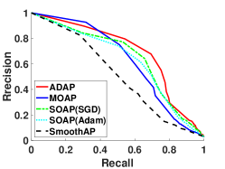
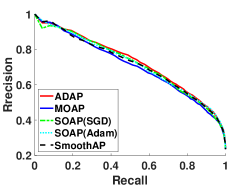
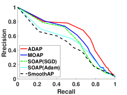
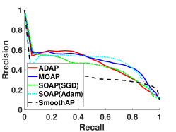
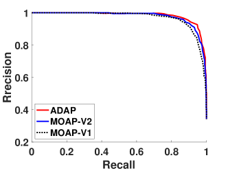
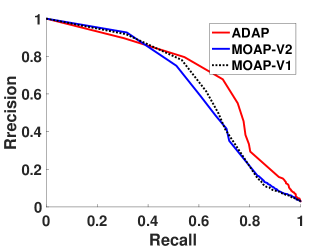
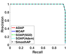
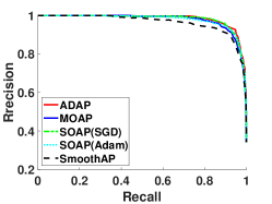
Figure 1: Precision-Recall curves of the Final models on the testing set

Table 3: Final averaged AP scores on the testing data.

Method	mushrooms	phishing	w6a
MOAP	$0.999\pm 2$E-$6$	$0.978\pm 2$E-$6$	$0.596\pm 2$E-$3$
ADAP	${\bf 1}$	${\bf 0.981\pm 2}$E-${\bf 7}$	${\bf 0.675\pm 1}$E-${\bf 4}$
SOAP (SGD)	$0.997\pm 1$E-$5$	$0.978\pm 4$E-$6$	$0.612\pm 4$E-$5$
SOAP (Adam)	$1$	$0.977\pm 1$E-$6$	$0.592\pm 3$E-$4$
SmoothAP	$0.962\pm 1$E-$3$	$0.967\pm 8$E-$6$	$0.473\pm 1$E-$4$
Method	a9a	w8a	ijcnn1
MOAP	$0.715\pm 3$E-$5$	$0.584\pm 4$E-$4$	$0.471\pm 6$E-$4$
ADAP	${\bf 0.730\pm 1}$E-${\bf 6}$	${\bf 0.659\pm 5}$E-${\bf 4}$	$0.536\pm 1$E-$3$
SOAP (SGD)	$0.714\pm 3$E-$5$	$0.561\pm 1$E-$3$	$0.476\pm 2$E-$4$
SOAP (Adam)	$0.721\pm 1$E-$5$	$0.475\pm 2$E-$3$	${\bf 0.547\pm 1}$E-${\bf 3}$
SmoothAP	$0.713\pm 3$E-$5$	$0.459\pm 3$E-$4$	$0.374\pm 3$E-$4$

(a) mushrooms dataset

(b) phishing dataset

(c) w6a dataset

(d) a9a dataset

(e) w8a dataset

(f) ijcnn1 dataset

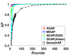
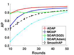
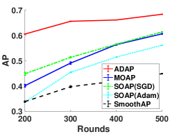
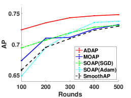
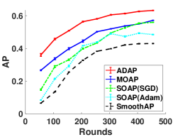
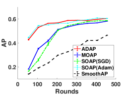
Figure 2: AP vs # of rounds on the training set

Results

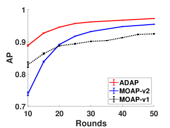
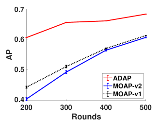
. The convergence curves of AP on training examples are reported in Figure 2, and the final AP scores on the testing data are shown in Table 3. We also plot the Precision-Recall curves of the final models on testing data in Figure 1. From Figure 2, we can see that the proposed ADAP converges faster than other methods. MOAP converges faster than SOAP on mushrooms, phishing, and w8a, and has similar performance as SOAP on other three datasets. From Table 3, we can see that ADAP has the best performance on all data sets except ijcnn1, on which ADAP is similar to SOAP (Adam). These results verify the effectiveness of the proposed methods, in particular the adaptive method ADAP.

Table 4: Test AUPRC on CIFAR10 and CIFAR100.

Method	CIFAR10	CIFAR100
ADAP	$\mathbf{0.7667\pm 0.0015}$	$\mathbf{0.6371\pm 0.0041}$
SOAP (Adam)	$0.7629\pm 0.0014$	$0.6251\pm 0.0053$
SmoothAP	$0.7365\pm 0.0088$	$0.6071\pm 0.0064$

4.2 Training Deep Neural Networks

Next, we present empirical results on optimizing deep neural networks. We mainly focus on comparing the performance of our proposed ADAP (Adam-style) algorithm with the two state-of-the-art algorithms, i.e., SmoothAP [4] and SOAP (Adam) [44].

Datasets.

Following [44], we conduct experiments on the imbalanced binary-class version of CIFAR10 and CIFAR100 datasets, which are constructed as follows: Firstly, half of the classes in the original CIFAR10 and CIFAR100 datasets are designated to be the positive class, and the rest half of classes are considered to be the negative class. Then, we remove $98\%$ of the positive examples in the training set to make it imbalanced, while keeping the test set unchanged. Finally, the training data set is splited into train/validation sets as a $4:1$ ratio.

Configurations.

We choose ResNet-18 [25] to be the neural network for our imbalanced binary image classification task. Before the training process, similar to [44], the ResNet-18 model is initialized with a model pretrained by the Adam optimizer for optimizing the cross entropy loss, whose learning rate and weight decay parameter are searched in $\{10^{-6},10^{-5},10^{-4}\}$. Then, the last layer of the neural network is re-initialized and the network is trained by different AP maximization methods, with hyper-parameters individually tuned for fair comparison. For SOAP and ADAP, we tune the $\beta_{0}$ parameter in range $\{0.001,0.1,0.5,0.9,0.99,0.999\}$, the margin parameter $m$ in $\{0.5,1,2,5,10\}$, and learning rate $\eta$ in $\{10^{-6},10^{-5},10^{-4}\}$.

Results

We conduct each experiment for 5 times, and report the mean test AUPRC as well as the standard variation in Table 4. We could observe that our proposed ADAP enjoys the best results on both datasets.

5 CONCLUSION AND FUTURE WORK

In this paper, we investigate the stochastic optimization of AUPRC by maximizing a surrogate loss of AP, which is one of the most important performance metrics for imbalanced classification problems. Previous study has shown that an $O(1/\epsilon^{5})$ convergence rate can be achieved. In this work, we further improve the theoretical guarantee by proposing a stochastic momentum method as well as a family of adaptive methods, which enjoy a better convergence rate of $O(1/\epsilon^{4})$. Our essential ideas the are two-folds: (i) updating the biased estimator for individual ranking-scores-tracking in a randomized coordinate-wise manner; (ii) applying the momentum step on top of the stochastic gradient estimator for tracking the gradient of the objective. Empirical studies on optimizing linear models and deep networks show the effectiveness of the proposed adaptive methods. For future work, we consider applying the proposed algorithms to other deep learning tasks.

Acknowledgements

T. Yang was was partially supported by NSF Career Award $\#$1844403, NSF Award $\#$2110545, NSF Award $\#$1933212. L. Zhang was partially supported by JiangsuSF (BK20200064).

A NOTATIONS

We first introduce the following lemma, which demonstrates the basic properties of the functions in our optimization problem (4).

Lemma 1.

Suppose Assumptions 1 and 2 hold, then there exist $G,C_{g},L_{g},C_{f},L_{f},C_{F},L_{F}>0$, such that $\forall\mathbf{w},$ $\|g_{i}(\mathbf{w})\|^{2}\leq G^{2}$, $g_{i}(\mathbf{w})$ is $C_{g}$-Lipschitz and $L_{g}$-smooth, and $\forall\mathbf{u}\in\Omega,$ $f(\mathbf{u})$ is $C_{f}$-Lipschitz and $L_{f}$-smooth. Finally, $\forall\mathbf{w}$, $F(\mathbf{w})$ is $C_{F}$-Lipschiz and $L_{F}$-smooth.

Proof.

For $g_{i}(\mathbf{w})$, we have $\|g_{i}(\mathbf{w})\|^{2}\leq m^{2}M^{2}+n^{2}M^{2}=G^{2}$, $\|\nabla g_{i}(\mathbf{w})\|^{2}\leq m^{2}\sigma^{2}+n^{2}\sigma^{2}=C_{g}^{2}$, and $\|\nabla g_{i}(\mathbf{w})-\nabla g_{i}(\mathbf{w}^{\prime})\|^{2}\leq m^{2}L_{l}^{2}\|\mathbf{w}-\mathbf{w}^{\prime}\|^{2}+n^{2}L_{l}^{2}\|\mathbf{w}-\mathbf{w}^{\prime}\|^{2}=L_{g}^{2}\|\mathbf{w}-\mathbf{w}^{\prime}\|^{2}$. Similarly, for $f(\mathbf{u})$, we have $\|\nabla f(\mathbf{u})\|_{2}^{2}=\|(\frac{-1}{u_{2}},\frac{u_{1}}{u_{2}^{2}})\|^{2}\leq 1/C^{2}+M^{2}m^{2}/C^{2}=C_{f}^{2}$ and $\|\nabla f(\mathbf{u})-\nabla f(\mathbf{u}^{\prime})\|_{2}^{2}=\|(\frac{-1}{u_{2}}-\frac{-1}{u_{2}^{\prime}},\frac{u_{1}}{u_{2}^{2}}-\frac{u_{1}^{\prime}}{u_{2}^{{}^{\prime}2}})\|^{2}\leq\frac{(u_{2}-u_{2}^{\prime})^{2}}{C^{2}}+\frac{2(u_{1}-u_{1}^{\prime})^{2}}{C^{4}}+\frac{8(Mm)^{2}(Mn)^{2}(u_{2}-u_{2}^{\prime})^{2}}{C^{8}}\leq L_{f}^{2}(\|\mathbf{u}-\mathbf{u}^{\prime}\|^{2})$ for any $\mathbf{u},\mathbf{u}^{\prime}\in\Omega$. Hence, $f(g_{i}(\mathbf{w}))$ is $C_{F}=(C_{g}C_{f})$-Lipschitz, and $L_{F}=(C_{g}^{2}L_{f}+L_{g}C_{f})$-smooth. Since $F(\mathbf{w})$ is the average of $f(g_{i}(\mathbf{w}))$, it is also $C_{F}$-Lipschitz and $L_{F}$-smooth. ∎

B PROOF OF THEOREM 1

Let $\Delta_{t}=\mathbf{m}_{t+1}-\nabla F(\mathbf{w}_{t}).$ According to the update rule in Algorithm 1, and we have

$$\begin{split}\|\Delta_{t}\|^{2}=&\left\|(1-\beta_{1})\mathbf{m}_{t}+\beta_{1}\frac{1}{m}\sum_{i=1}^{m}\nabla\tilde{g}_{i}(\mathbf{w}_{t})^{\top}\cdot\nabla f\left([U_{t+1}]^{\top}_{i}\right)-\nabla F(\mathbf{w}_{t})\right\|^{2}\\ =&\Bigg{\|}\underbrace{(1-\beta_{1})[\mathbf{m}_{t}-\nabla F(\mathbf{w}_{t-1})]}_{A_{1}}+\underbrace{(1-\beta_{1})[\nabla F(\mathbf{w}_{t-1})-\nabla F(\mathbf{w}_{t})]}_{A_{2}}\\ &+\underbrace{\beta_{1}\left[\frac{1}{m}\sum_{i=1}^{m}\nabla\tilde{g}_{i}(\mathbf{w}_{t})^{\top}\cdot\nabla f\left([U_{t+1}]^{\top}_{i}\right)-\frac{1}{m}\sum_{i=1}^{m}\nabla\tilde{g}_{i}(\mathbf{w}_{t})^{\top}\cdot\nabla f\left(g_{i}(\mathbf{w}_{t})\right)\right]}_{A_{3}}\\ &+\underbrace{\beta_{1}\left[\frac{1}{m}\sum_{i=1}^{m}\nabla\tilde{g}_{i}(\mathbf{w}_{t})^{\top}\cdot\nabla f\left(g_{i}(\mathbf{w}_{t})\right)-\nabla F(\mathbf{w}_{t})\right]}_{A_{4}}\Bigg{\|}^{2}.\end{split}$$ (14)

Let $\mathrm{E}_{t}[\cdot]=\mathrm{E}[\cdot|\mathcal{F}_{t-1}]$, where $\mathcal{F}_{t-1}$ is the $\sigma$-algebra of MOAP-V1, which contains the learning history from round 1 to round $t-1$. Since $\tilde{g}_{t}(\mathbf{w})$ is an unbiased estimator of $g_{i}(\mathbf{w})$, we have $\mathrm{E}_{t}[A_{4}]=0$. Moreover, $A_{1}$ and $A_{2}$ are fixed given $\mathcal{F}_{t-1}$. Thus

$$\begin{split}{}&\mathrm{E}_{t}[\|\Delta_{t}\|^{2}]\\ \leq{}&\mathrm{E}_{t}[\|A_{1}+A_{2}+A_{3}\|^{2}]+\mathrm{E}_{t}[\|A_{4}\|^{2}]+2\mathrm{E}_{t}[\|A_{3}\|\|A_{4}\|]+\underbrace{2(A_{1}+A_{2})^{\top}\mathrm{E}_{t}[A_{4}]}_{=0}\\ \leq{}&\mathrm{E}_{t}[\|A_{1}+A_{2}+A_{3}\|^{2}]+2\mathrm{E}_{t}[\|A_{4}\|^{2}]+\mathrm{E}_{t}[\|A_{3}\|^{2}]\\ \leq{}&(1+\beta_{1})\mathrm{E}_{t}[\|A_{1}\|^{2}]+\left(1+\frac{1}{\beta_{1}}\right)\mathrm{E}_{t}[\|A_{2}+A_{3}\|^{2}]+2\mathrm{E}_{t}[\|A_{4}\|^{2}]+\mathrm{E}_{t}[\|A_{3}\|^{2}]\\ \leq{}&{(1+\beta_{1}^{2})}(1-\beta_{1})\|\Delta_{t-1}\|^{2}+\frac{2(1+\beta_{1})}{\beta_{1}}\|A_{2}\|^{2}+\frac{2+3\beta_{1}}{\beta_{1}}\mathrm{E}_{t}[\|A_{3}\|^{2}]+2\mathrm{E}_{t}[\|A_{4}\|^{2}],\end{split}$$ (15)

where the third inequality is based on Young’s inequality. To proceed, according to Lemma 1, we have

$$\|A_{2}\|^{2}=(1-\beta_{1})^{2}\|\nabla F(\mathbf{w}_{t-1})-\nabla F(\mathbf{w}_{t})\|^{2}\leq(1-\beta_{1})^{2}L^{2}_{F}\|\mathbf{w}_{t}-\mathbf{w}_{t-1}\|^{2},$$ (16)

$$\begin{split}\|A_{3}\|^{2}\leq{}&\beta_{1}^{2}\frac{1}{m}\sum_{i=1}^{m}\|\nabla\tilde{g}_{i}(\mathbf{w}_{t})^{\top}\cdot\nabla f\left([U_{t+1}]^{\top}_{i}\right)-\nabla\tilde{g}_{i}(\mathbf{w}_{t})^{\top}\cdot\nabla f\left(g_{i}(\mathbf{w}_{t})\right)\|^{2}\\ \leq{}&\beta_{1}^{2}\frac{C_{g}^{2}}{m}\sum_{i=1}^{m}\|\nabla f([U_{t+1}]^{\top}_{i})-\nabla f(g_{i}(\mathbf{w}_{t}))\|^{2}\\ \leq{}&\beta_{1}^{2}\frac{C^{2}_{g}L^{2}_{f}}{m}\sum_{i=1}^{m}\|[U_{t+1}]_{i}^{\top}-g_{i}(\mathbf{w}_{t})\|^{2}={}\frac{\beta_{1}^{2}C_{g}^{2}L^{2}_{f}}{m}\|U_{t+1}-g(\mathbf{w}_{t})\|^{2},\end{split}$$ (17)

where $g(\mathbf{w}_{t})=[g_{1}(\mathbf{w}_{t}),\dots,g_{m}(\mathbf{w}_{t})]^{\top}$, and

$$\mathrm{E}_{t}[\|A_{4}\|^{2}]\leq{}\beta_{1}^{2}\mathrm{E}_{t}\left[\left\|\frac{1}{m}\sum_{i=1}^{m}\nabla\tilde{g}_{i}(\mathbf{w}_{t})^{\top}\cdot\nabla f([U_{t+1}]_{i}^{\top})\right\|^{2}\right]\leq\beta_{1}^{2}C_{g}^{2}C_{f}^{2}.$$ (18)

Combining (LABEL:eqn:appendix:theorem:A1), (16), (17), (18), we get

$$\begin{split}\mathrm{E}_{t}[\|\Delta_{t}\|^{2}]\leq{}&(1-\beta_{1})\|\Delta_{t-1}\|^{2}+\frac{2L_{F}^{2}\|\mathbf{w}_{t}-\mathbf{w}_{t-1}\|^{2}}{\beta_{1}}+\frac{5\beta_{1}C_{g}^{2}L^{2}_{f}\mathrm{E}_{t}[\|U_{t+1}-g(\mathbf{w}_{t})\|^{2}]}{m}\\ {}&+2\beta_{1}^{2}C_{g}^{2}C_{f}^{2}.\end{split}$$ (19)

Summing over from 1 to $T$, we get

$$\begin{split}\mathrm{E}\left[\sum_{i=1}^{T}\|\Delta_{i}\|^{2}\right]\leq&\frac{\|\Delta_{0}\|^{2}}{\beta_{1}}+\frac{2L_{F}^{2}\sum_{i=1}^{T}\|\mathbf{w}_{i}-\mathbf{w}_{i-1}\|^{2}}{\beta_{1}^{2}}+\frac{5C_{g}^{2}L^{2}_{f}\sum_{i=1}^{T}\mathrm{E}_{i}[\|U_{i+1}-g(\mathbf{w}_{i})\|^{2}]}{m}\\ &+2\beta_{1}C_{g}^{2}C_{f}^{2}T\\ =&\frac{2C_{F}^{2}}{\beta_{1}}+\frac{2L_{F}^{2}\eta^{2}\sum_{i=1}^{T}\|\mathbf{m}_{i}\|^{2}}{\beta^{2}}+\frac{5C_{g}^{2}L^{2}_{f}\sum_{i=1}^{T}\mathrm{E}_{i}[\|U_{i+1}-g(\mathbf{w}_{i})\|^{2}]}{m}\\ &+2\beta_{1}C_{g}^{2}C_{f}^{2}T\end{split}$$ (20)

Note that here $\mathbf{w}_{0}$ can be considered as a psudo-decision which follows the same update procedure as $\mathbf{w}_{t}$. Next, we turn to bound the third term of the R.H.S. of the inequality, and introduce the following lemma.

Lemma 2 (Variance Recursion [50]).

Consider a sequence $\mathbf{m}_{t+1}=(1-\beta)\mathbf{m}_{t}+\beta\tilde{h}(\mathbf{w}_{t})$ for tracking $h(\mathbf{w}_{t})$, where $\mathrm{E}[\tilde{h}(\mathbf{w}_{t})]=h(\mathbf{w}_{t})$ and $h$ is a $C$-Lipchitz continuous mapping. Then we have

$$\mathrm{E}_{t}[\|\mathbf{m}_{t+1}-h(\mathbf{w}_{t})\|^{2}]\leq(1-\beta)\|\mathbf{m}_{t}-h(\mathbf{w}_{t-1})\|^{2}+\beta^{2}\mathrm{E}_{t}[\|\tilde{h}(\mathbf{w}_{t})-h(\mathbf{w}_{t})\|^{2}]+\frac{2C^{2}\|\mathbf{w}_{t}-\mathbf{w}_{t-1}\|^{2}}{\beta}.$$ (21)

With Lemma 2, we have

$$\sum_{i=1}^{T}\mathrm{E}_{i}[\|U_{i+1}-g(\mathbf{w}_{i})\|^{2}]\leq\frac{mG^{2}}{\beta_{0}}+2\beta_{0}TmG^{2}+\frac{2mC^{2}_{g}\eta^{2}\sum_{i=1}^{T}\|\mathbf{m}_{i}\|^{2}}{\beta_{0}^{2}}.$$ (22)

Combining all the about results together, and set $\beta_{0}=\beta_{1}=\beta$, we have

$$\begin{split}\mathrm{E}\left[\sum_{i=1}^{T}\|\Delta_{i}\|^{2}\right]\leq{}&\frac{2C_{F}^{2}+5C_{g}^{2}L_{f}^{2}G^{2}}{\beta}+\frac{(2L_{F}^{2}+10C_{g}^{4}L_{f}^{2})\eta^{2}}{\beta^{2}}\sum_{i=1}^{T}\|\mathbf{m}_{i}\|^{2}\\ {}&+\beta(10C_{g}^{2}L_{f}^{2}G^{2}+2C_{g}^{2}C_{f}^{2})T.\end{split}$$ (23)

We introduce the following lemma [24], which can be obtained following the definition of the smoothness.

Lemma 3.

Consider a sequence $\mathbf{w}_{t+1}=\mathbf{w}_{t}-\eta\mathbf{m}_{t+1}$ for a $L_{F}$-smooth function $F$, with $\eta L_{F}\leq 1/2$ we have

$$F(\mathbf{w}_{t+1})\leq F(\mathbf{w}_{t})+\frac{\eta}{2}\|\nabla F(\mathbf{w}_{t})-\mathbf{m}_{t+1}\|^{2}-\frac{\eta}{2}\|\nabla F(\mathbf{w}_{t})\|^{2}-\frac{\eta}{4}\|\mathbf{m}_{t+1}\|^{2}.$$

Based on Lemma 3, with $(2L_{F}^{2}+10C_{g}^{4}L_{f}^{2})\eta^{2}/\beta^{2}\leq 1/2$, we get

$$\begin{split}\mathrm{E}\left[\frac{1}{T}\sum_{t=1}^{T}\|\nabla F_{\mathbf{w}}(\mathbf{w}_{t})\|^{2}\right]\leq{}&\frac{2(F(\mathbf{w}_{T+1})-F(\mathbf{w}_{1}))}{\eta T}+\frac{C_{F}^{2}+5C_{g}^{2}L_{f}^{2}G^{2}}{\beta T}\\ {}&+\beta(10C_{g}^{2}L_{f}^{2}G^{2}+2C_{g}^{2}C_{f}^{2}).\end{split}$$ (24)

Thus, by setting $\beta=O(\epsilon^{2})$ and $\eta=O(\beta)$, we have $\mathrm{E}\left[\frac{1}{T}\sum_{t=1}^{T}\|\nabla F_{\mathbf{w}}(\mathbf{w}_{t})\|^{2}\right]=O(\epsilon^{2})$ for

$$T\geq\max\left\{\frac{2(F(\mathbf{w}_{1})-F(\mathbf{w}_{T+1}))}{\eta\epsilon^{2}},\frac{C_{F}^{2}+10C_{g}^{2}L_{f}^{2}G^{2}}{\beta\epsilon^{2}}\right\}.$$

C PROOF OF THEOREM 2

Let $i_{t}$ be the positive data chosen in round $t$, and for convenience we set $\beta_{0}=\beta_{1}=\beta$. According to the update rule in Algorithm 1, and we have

$$\begin{split}\|\Delta_{t}\|^{2}=&\left\|(1-\beta)\mathbf{m}_{t}+\beta\nabla\tilde{g}_{i_{t}}(\mathbf{w}_{t})^{\top}\cdot\nabla f\left([U_{t+1}]^{\top}_{i_{t}}\right)-\nabla F(\mathbf{w}_{t})\right\|^{2}\\ =&\Bigg{\|}\underbrace{(1-\beta)[\mathbf{m}_{t}-\nabla F(\mathbf{w}_{t-1})]}_{A_{1}}+\underbrace{(1-\beta)[\nabla F(\mathbf{w}_{t-1})-\nabla F(\mathbf{w}_{t})]}_{A_{2}}\\ &+\underbrace{\beta\left[\nabla\tilde{g}_{i_{t}}(\mathbf{w}_{t})^{\top}\cdot\nabla f\left([U_{t+1}]^{\top}_{i_{t}}\right)-\nabla\tilde{g}_{i_{t}}(\mathbf{w}_{t})^{\top}\cdot\nabla f\left(g_{i_{t}}(\mathbf{w}_{t})\right)\right]}_{A_{3}}\\ &+\underbrace{\beta\left[\nabla\tilde{g}_{i_{t}}(\mathbf{w}_{t})^{\top}\cdot\nabla f\left(g_{i_{t}}(\mathbf{w}_{t})\right)-\nabla F(\mathbf{w}_{t})\right]}_{A_{4}}\Bigg{\|}^{2}.\end{split}$$ (25)

Thus

$$\begin{split}{}&\mathrm{E}_{t}[\|\Delta_{t}\|^{2}]\leq(1-\beta)\|\Delta_{t-1}\|^{2}+\frac{2(1+\beta)}{\beta}\|A_{2}\|^{2}+\frac{2+3\beta}{\beta}\mathrm{E}_{t}[\|A_{3}\|^{2}]+2\mathrm{E}_{t}[\|A_{4}\|^{2}],\end{split}$$ (26)

where

$$\|A_{2}\|^{2}=(1-\beta_{1})^{2}\|\nabla F(\mathbf{w}_{t-1})-\nabla F(\mathbf{w}_{t})\|^{2}\leq(1-\beta_{1})^{2}L^{2}_{F}\|\mathbf{w}_{t}-\mathbf{w}_{t-1}\|^{2},$$ (27)

$$\begin{split}\|A_{3}\|^{2}\leq{}&\beta^{2}\|\nabla\tilde{g}_{i_{t}}(\mathbf{w}_{t})^{\top}\cdot\nabla f\left([U_{t+1}]^{\top}_{i_{t}}\right)-\nabla\tilde{g}_{i_{t}}(\mathbf{w}_{t})^{\top}\cdot\nabla f\left(g_{i_{t}}(\mathbf{w}_{t})\right)\|^{2}\\ \leq{}&\beta^{2}{C_{g}^{2}}\|\nabla f([U_{t+1}]^{\top}_{i_{t}})-\nabla f(g_{i_{t}}(\mathbf{w}_{t}))\|^{2}\\ \leq{}&\beta^{2}{C^{2}_{g}L^{2}_{f}}\|[U_{t+1}]_{i_{t}}^{\top}-g_{i_{t}}(\mathbf{w}_{t})\|^{2},\end{split}$$ (28)

and

$$\mathrm{E}[\|A_{4}\|^{2}]\leq{}\beta^{2}\mathrm{E}[\|\nabla\tilde{g}_{i_{t}}(\mathbf{w}_{t})^{\top}\cdot\nabla f([U_{t+1}]_{i_{t}}^{\top})\|^{2}]\leq\beta_{1}^{2}C_{g}^{2}C_{f}^{2}.$$ (29)

Combining the results above, we get

$$\begin{split}\mathrm{E}[\|\Delta_{t}\|^{2}]\leq{}&(1-\beta)\|\Delta_{t-1}\|^{2}+\frac{2L_{F}^{2}\|\mathbf{w}_{t}-\mathbf{w}_{t-1}\|^{2}}{\beta_{1}}+{5\beta C_{g}^{2}L^{2}_{f}\mathrm{E}[\|[U_{t+1}]_{i_{t}}-g_{i_{t}}(\mathbf{w}_{t})\|^{2}]}\\ {}&+2\beta^{2}C_{g}^{2}C_{f}^{2}.\end{split}$$ (30)

Next, we turn to bound the third term on the R.H.S. of (30). Following [44], we divide the whole interval into $m$ groups, with the $i$-th group $\mathcal{T}_{i}=\{t_{1}^{i},\dots,t_{k}^{i},\dots\}$, where $t_{k}^{i}$ denotes the $k$-th time that the $i$-th positive data is chosen to update $[U_{t_{k}^{i}}]_{i}$ and obtain $[U_{t_{k}^{i}+1}]_{i}$. Note that since we only update the chosen data, we have $[U_{t_{k}^{i}+1}]_{i}=\dots=[U_{t_{k+1}^{i}}]_{i}$. Without loss of generality, assume $i_{t}$ is picked for the $k$-th time at round $t$. Thus

$$\begin{split}&\mathrm{E}[\|[U_{t+1}]_{i_{t}}-g_{i_{t}}(\mathbf{w}_{t})\|^{2}]\\ ={}&\mathrm{E}[\|[U_{t_{k}^{i_{t}}+1}]_{i_{t}}-g_{i_{t}}(\mathbf{w}_{t_{k}^{i_{t}}})\|^{2}]\\ \leq{}&\mathrm{E}[\|(1-\beta)[U_{t^{i_{t}}_{k-1}+1}]_{i_{t}}+\beta\tilde{g}_{i}(\mathbf{w}_{t^{i_{t}}_{k}})-g_{i_{t}}(\mathbf{w}_{t_{k}^{i_{t}}})\|^{2}]\\ ={}&\mathrm{E}[\|(1-\beta)([U_{t_{k-1}^{i_{t}}+1}]_{i_{t}}-g_{i_{t}}(\mathbf{w}_{t_{k-1}^{i_{t}}}))+\beta(\tilde{g}_{i_{t}}(\mathbf{w}_{t_{k-1}^{i_{t}}})-g_{i_{t}}(\mathbf{w}_{t_{k-1}^{i_{t}}}))+g_{i_{t}}(\mathbf{w}_{t_{k-1}^{i_{t}}})-g_{i_{t}}(\mathbf{w}_{t_{k}^{i_{t}}})\|^{2}]\\ \leq{}&(1+\beta)(1-\beta)^{2}\mathrm{E}[\|[U_{t_{k-1}^{i_{t}}+1}]_{i_{t}}-g_{i_{t}}(\mathbf{w}_{t_{k-1}^{i_{t}}})\|^{2}]+2(1+1/\beta)\beta^{2}\cdot 2G^{2}\\ {}&+2(1+1/\beta)\mathrm{E}[\|g_{i_{t}}(\mathbf{w}_{t_{k-1}^{i_{t}}})-g_{i_{t}}(\mathbf{w}_{t_{k}^{i_{t}}})\|^{2}]\\ \leq{}&(1-\beta)\mathrm{E}[\|[U_{t_{k-1}^{i_{t}}+1}]_{i_{t}}-g_{i_{t}}(\mathbf{w}_{t_{k-1}^{i_{t}}})\|^{2}]+8\beta G^{2}+\frac{4C_{g}^{2}}{\beta}\mathrm{E}[\|\mathbf{w}_{t_{k-1}^{i_{t}}}-\mathbf{w}_{t_{k}^{i_{t}}}\|^{2}]\\ \leq{}&(1-\beta)\mathrm{E}[\|[U_{t_{k-1}^{i_{t}}+1}]_{i_{t}}-g_{i_{t}}(\mathbf{w}_{t_{k-1}^{i_{t}}})\|^{2}]+8\beta G^{2}+\frac{4C_{g}^{2}\eta^{2}}{\beta}\mathrm{E}\left[\left\|\sum_{j=t^{i_{t}}_{k-1}+1}^{t_{k}^{i_{t}}}\mathbf{m}_{t}\right\|^{2}\right]\\ \leq{}&(1-\beta)\mathrm{E}[\|[U_{t_{k-1}^{i_{t}}+1}]_{i_{t}}-g_{i_{t}}(\mathbf{w}_{t_{k-1}^{i_{t}}})\|^{2}]+8\beta G^{2}+\frac{4C_{g}^{2}\eta^{2}}{\beta}\mathrm{E}\left[(t_{k}^{i_{t}}-t_{k-1}^{i_{t}})\sum_{j=t^{i_{t}}_{k-1}+1}^{t_{k}^{i_{t}}}\left\|\mathbf{m}_{j}\right\|^{2}\right]\end{split}$$ (31)

where the second and last inequalities are based on Young’s inequality. Note that, based on Lemma 1 of [44], $t_{k}^{i_{t}}-t_{k-1}^{i_{t}}$ is a random variable with conditional distribution given by a geometric distribution with $p=1/m$, i.e., $\mathrm{E}[t_{k}^{i_{t}}-t_{k-1}^{i_{t}}|t_{k-1}^{i_{t}}]\leq m$. However, since $t_{k}^{i_{t}}-t_{k-1}^{i_{t}}$ and $\sum_{j=t^{i_{t}}_{k-1}+1}^{t_{k}^{i_{t}}}\left\|\mathbf{m}_{j}\right\|^{2}$ are dependent, this conclusion can not be applied to bound the last term, which further making the advantages of the momentum can not be used. Because of this issue, we have to rewrite (LABEL:eqn:th2:356) and bound the last term as

$$\begin{split}\mathrm{E}\left[\left\|\sum_{j=t^{i_{t}}_{k-1}+1}^{t_{k}^{i_{t}}}\mathbf{m}_{t}\right\|^{2}\right]\leq C_{F}^{2}\mathrm{E}[(t_{k}^{i_{t}}-t_{k-1}^{i_{t}})^{2}]\leq 2m^{2}C_{F}^{2}.\end{split}$$ (32)

Thus

$$\mathrm{E}[\|[U_{t_{k}^{i_{t}}+1}]_{i_{t}}-g_{i_{t}}(\mathbf{w}_{t_{k}^{i_{t}}})\|^{2}]\leq(1-\beta)\mathrm{E}[\|[U_{t_{k-1}^{i_{t}}}]_{i_{t}}-g_{i_{t}}(\mathbf{w}_{t_{k-1}^{i_{t}}})\|^{2}]+8\beta G^{2}+\frac{8m^{2}C_{F}^{2}C_{g}^{2}\eta^{2}}{\beta}.$$

Summing over for all intervals, we have

$$\sum_{i=1}^{m}\mathrm{E}[\sum_{k=1}^{K_{i}}\|[U_{t_{k-1}^{i}}]_{i}-g_{i}(\mathbf{w}_{t_{k-1}^{i}})\|^{2}]\leq\frac{mG^{2}}{\beta}+8G^{2}T+\frac{8m^{2}C_{F}^{2}C_{g}^{2}\eta^{2}T}{\beta^{2}}$$

where $K_{i}$ denotes that the $i$-th positive data is chosen for $K_{i}$ times. Combining with (30), we get

$$\begin{split}\mathrm{E}[\sum_{i=1}^{T}\|\Delta_{i}\|^{2}]\leq\frac{2L_{f}^{2}\eta^{2}C_{F}^{2}T}{\beta^{2}}+\frac{40C_{g}^{4}L_{f}^{2}m^{2}C_{F}^{2}\eta^{2}T}{\beta}+\frac{C_{F}^{2}}{\beta}+5C_{g}^{2}L_{f}^{2}mG^{2}+\beta T(40C_{G}^{2}L_{f}^{2}G^{2}+8C_{g}^{2}C_{f}^{2}).\end{split}$$ (33)

With Lemma 3, we obtain

$$\begin{split}\mathrm{E}\left[\frac{1}{T}\sum_{i=1}^{T}\|\nabla F(\mathbf{w})\|^{2}\right]\leq{}&\frac{2(F(\mathbf{w}_{1})-F(\mathbf{w}_{T+1}))}{\eta T}+\frac{2L_{f}^{2}\eta^{2}C_{F}^{2}}{\beta^{2}}+\frac{40C_{g}^{4}L_{f}^{2}m^{2}C_{F}^{2}\eta^{2}}{\beta}\\ {}&+\frac{C_{F}^{2}}{\beta T}+\frac{5C_{g}^{2}L_{f}^{2}mG^{2}}{T}+\beta(40C_{G}^{2}L_{f}^{2}G^{2}+8C_{g}^{2}C_{f}^{2}).\end{split}$$ (34)

Finally, we can obtain a $\epsilon$-stationary solution by setting $\beta=O(\epsilon^{2})$, $\eta=O(\epsilon^{3}/m)$, and

$$T\geq\left\{\frac{2(F(\mathbf{w}_{1})-F(\mathbf{w}_{T+1}))}{\eta\epsilon^{2}},\frac{C_{F}^{2}}{\beta\epsilon^{2}},\frac{5C_{g}^{2}L_{f}^{2}mG^{2}}{\epsilon^{2}}\right\}.$$

D PROOF OF THEOREM 3

Let $\Delta_{t}=\mathbf{m}_{t+1}-\nabla F(\mathbf{w}_{t}).$ According to the update rule in Algorithm 2, and we have

$$\begin{split}\|\Delta_{t}\|^{2}=&\left\|(1-\beta_{1})\mathbf{m}_{t}+\beta_{1}\frac{1}{B}\sum_{\mathbf{x}_{i}\in\mathcal{B}_{t}}\nabla\tilde{g}_{i}(\mathbf{w}_{t})^{\top}\cdot\nabla f\left([U_{t+1}]^{\top}_{i}\right)-\nabla F(\mathbf{w}_{t})\right\|^{2}\\ =&\Bigg{\|}\underbrace{(1-\beta_{1})[\mathbf{m}_{t}-\nabla F(\mathbf{w}_{t-1})]}_{A_{1}}+\underbrace{(1-\beta_{1})[\nabla F(\mathbf{w}_{t-1})-\nabla F(\mathbf{w}_{t})]}_{A_{2}}\\ &+\underbrace{\beta_{1}\left[\frac{1}{B}\sum_{\mathbf{x}_{i}\in\mathcal{B}_{t}}\nabla\tilde{g}_{i}(\mathbf{w}_{t})^{\top}\cdot\nabla f\left([U_{t+1}]^{\top}_{i}\right)-\frac{1}{B}\sum_{\mathbf{x}_{i}\in\mathcal{B}_{t}}\nabla\tilde{g}_{i}(\mathbf{w}_{t})^{\top}\cdot\nabla f\left(g_{i}(\mathbf{w}_{t})\right)\right]}_{A_{3}}\\ &+\underbrace{\beta_{1}\left[\frac{1}{B}\sum_{\mathbf{x}_{i}\in\mathcal{B}_{t}}\nabla\tilde{g}_{i}(\mathbf{w}_{t})^{\top}\cdot\nabla f\left(g_{i}(\mathbf{w}_{t})\right)-\nabla F(\mathbf{w}_{t})\right]}_{A_{4}}\Bigg{\|}^{2}.\end{split}$$ (35)

Following similar procedure as in the proof of Theorem 1, we have

$$\begin{split}{}&\mathrm{E}_{t}[\|\Delta_{t}\|^{2}]\leq(1-\beta_{1})\|\Delta_{t-1}\|^{2}+\frac{2(1+\beta_{1})}{\beta_{1}}\|A_{2}\|^{2}+\frac{2+3\beta_{1}}{\beta_{1}}\mathrm{E}_{t}[\|A_{3}\|^{2}]+2\mathrm{E}_{t}[\|A_{4}\|^{2}],\end{split}$$ (36)

where

$$\|A_{2}\|^{2}=(1-\beta_{1})^{2}\|\nabla F(\mathbf{w}_{t-1})-\nabla F(\mathbf{w}_{t})\|^{2}\leq(1-\beta_{1})^{2}L^{2}_{F}\|\mathbf{w}_{t}-\mathbf{w}_{t-1}\|^{2}$$ (37)

$$\begin{split}\|A_{3}\|^{2}\leq{}&\beta_{1}^{2}\frac{1}{B}\sum_{\mathbf{x}_{i}\in\mathcal{B}_{t}}\|\nabla\tilde{g}_{i}(\mathbf{w}_{t})^{\top}\cdot\nabla f\left([U_{t+1}]^{\top}_{i}\right)-\nabla\tilde{g}_{i}(\mathbf{w}_{t})^{\top}\cdot\nabla f\left(g_{i}(\mathbf{w}_{t})\right)\|^{2}\\ \leq{}&\beta_{1}^{2}\frac{C_{g}^{2}}{B}\sum_{\mathbf{x}_{i}\in\mathcal{B}_{t}}\|\nabla f([U_{t+1}]^{\top}_{i})-\nabla f(g_{i}(\mathbf{w}_{t}))\|^{2}\\ \leq{}&\beta_{1}^{2}\frac{C^{2}_{g}L^{2}_{f}}{B}\sum_{\mathbf{x}_{i}\in\mathcal{B}_{t}}\|[U_{t+1}]_{i}^{\top}-g_{i}(\mathbf{w}_{t})\|^{2}\end{split}$$ (38)

and

$$\mathrm{E}_{t}[\|A_{4}\|^{2}]\leq{}\beta_{1}^{2}\mathrm{E}_{t}\left[\left\|\frac{1}{B}\sum_{\mathbf{x}_{i}\in\mathcal{B}_{t}}\nabla\tilde{g}_{i}(\mathbf{w}_{t})^{\top}\cdot\nabla f([U_{t+1}]_{i}^{\top})\right\|^{2}\right]\leq\beta_{1}^{2}C_{g}^{2}C_{f}^{2}.$$ (39)

Combining (LABEL:eqn:appendix:theorem:A1:3), (37), (38), (39), and taking expectation over the randomness of $\mathcal{B}_{t}$, we get

$$\begin{split}\mathrm{E}_{t}[\|\Delta_{t}\|^{2}]\leq{}&(1-\beta_{1})\|\Delta_{t-1}\|^{2}+\frac{2L_{F}^{2}\|\mathbf{w}_{t}-\mathbf{w}_{t-1}\|^{2}}{\beta_{1}}+\frac{5\beta_{1}C_{g}^{2}L^{2}_{f}\mathrm{E}_{t}[\|U_{t+1}-g(\mathbf{w}_{t})\|^{2}]}{m}\\ {}&+2\beta_{1}^{2}C_{g}^{2}C_{f}^{2}.\end{split}$$ (40)

Summing over from 1 to $T$ and taking the expectation with respect to all the randomness, we get

$$\begin{split}\mathrm{E}\left[\sum_{i=1}^{T}\|\Delta_{i}\|^{2}\right]\leq&\frac{\|\Delta_{0}\|^{2}}{\beta_{1}}+\frac{2L_{F}^{2}\sum_{i=1}^{T}\|\mathbf{w}_{i}-\mathbf{w}_{i-1}\|^{2}}{\beta_{1}^{2}}+\frac{5C_{g}^{2}L^{2}_{f}\sum_{i=1}^{T}\mathrm{E}_{i}[\|U_{i+1}-g(\mathbf{w}_{i})\|^{2}]}{m}\\ &+2\beta_{1}C_{g}^{2}C_{f}^{2}T\\ =&\frac{C_{F}^{2}}{\beta_{1}}+\frac{2L_{F}^{2}\eta^{2}\sum_{i=1}^{T}\|\mathbf{m}_{i}\|^{2}}{\beta^{2}}+\frac{5C_{g}^{2}L^{2}_{f}\sum_{i=1}^{T}\mathrm{E}_{i}[\|U_{i+1}-g(\mathbf{w}_{i})\|^{2}]}{m}\\ &+2\beta_{1}C_{g}^{2}C_{f}^{2}T.\end{split}$$ (41)

Next, note that $U_{t+1}=\Pi_{\Omega^{m}}[(1-\beta_{0})U_{t}+\beta_{0}\widehat{g}(\mathbf{w}_{t})]$, where $\widehat{g}(\mathbf{w}_{t})$ is an unbiased estimator of $g(\mathbf{w}_{t})$, which is defined in (12). Thus, with Lemma 2 and the fact that

$$\mathrm{E}[\|\widehat{g}(\mathbf{w}_{t})-g(\mathbf{w}_{t})\|^{2}]\leq\mathrm{E}[\|\widehat{g}(\mathbf{w}_{t})\|^{2}]=\mathrm{E}\left[\sum_{\mathbf{x}_{i}\in\mathcal{B}_{t}}\left\|\frac{m}{B}\tilde{g}_{i}(\mathbf{w})\right\|^{2}\right]\leq\frac{m^{2}}{B}G^{2}.$$

we have

$$\sum_{i=1}^{T}\mathrm{E}_{i}[\|U_{i+1}-g(\mathbf{w}_{i})\|^{2}]\leq\frac{mG^{2}}{\beta_{0}}+2\beta_{0}T\frac{m^{2}}{B}G^{2}+\frac{2mC^{2}_{g}\eta^{2}\sum_{i=1}^{T}\|\mathbf{m}_{i}\|^{2}}{\beta_{0}^{2}}.$$ (42)

Combining all the about results together, and set $\beta_{0}=\beta_{1}=\beta$, we have

$$\begin{split}\mathrm{E}\left[\sum_{i=1}^{T}\|\Delta_{i}\|^{2}\right]\leq{}&\frac{C_{F}^{2}+5C_{g}^{2}L_{f}^{2}G^{2}}{\beta}+\frac{(2L_{F}^{2}+10C_{g}^{4}L_{f}^{2})\eta^{2}}{\beta^{2}}\sum_{i=1}^{T}\|\mathbf{m}_{i}\|^{2}\\ {}&+\beta(10C_{g}^{2}L_{f}^{2}G^{2}\frac{m}{B}+2C_{g}^{2}C_{f}^{2})T.\end{split}$$ (43)

Based on Lemma 3, with $(2L_{F}^{2}+10C_{g}^{4}L_{f}^{2})\eta^{2}/\beta^{2}\leq 1/2$, we get

$$\begin{split}\mathrm{E}\left[\frac{1}{T}\sum_{t=1}^{T}\|\nabla F(\mathbf{w}_{t})\|^{2}\right]\leq{}&\frac{2(F(\mathbf{w}_{1})-F(\mathbf{w}_{T}))}{\eta T}+\frac{C_{F}^{2}+5C_{g}^{2}L_{f}^{2}G^{2}}{\beta T}\\ {}&+\beta(5C_{g}^{2}L_{f}^{2}G^{2}\frac{m}{B}+2C_{g}^{2}C_{f}^{2}).\end{split}$$ (44)

Thus, by setting $\beta=O(\epsilon^{2}B/m)$ and $\eta=O(\beta)$, we have $\mathrm{E}\left[\frac{1}{T}\sum_{t=1}^{T}\|\nabla F_{\mathbf{w}}(\mathbf{w}_{t})\|^{2}\right]=O(\epsilon^{2})$ for

$$T\geq\max\left\{\frac{2(F(\mathbf{w}_{1})-F(\mathbf{w}_{T+1}))}{\eta\epsilon^{2}},\frac{C_{F}^{2}+5C_{g}^{2}L_{f}^{2}G^{2}}{\beta\epsilon^{2}}\right\}.$$

E PROOF OF THEOREM 4

Let $\Delta_{t}=\mathbf{m}_{t+1}-\nabla F(\mathbf{w}_{t}),$ and $\eta^{s}_{t}=1/(\sqrt{\mathbf{v}_{t+1}}+\delta)$. Based on the boundedness of $\|tilde{\nabla}\|$, we know that $\eta c_{l}\leq[\eta^{s}_{t}]_{i}\leq\eta c_{u}$ for all $i\in[d]$. According to the update rule in Algorithm 3, we have

$$\begin{split}\|\Delta_{t}\|^{2}=&\left\|(1-\beta_{1})\mathbf{m}_{t}+\beta_{1}\frac{1}{B}\sum_{\mathbf{x}_{i}\in\mathcal{B}_{t}}\nabla\tilde{g}_{i}(\mathbf{w}_{t})^{\top}\cdot\nabla f\left([U_{t+1}]^{\top}_{i}\right)-\nabla F(\mathbf{w}_{t})\right\|^{2}\end{split}$$ (45)

Following similar procedure as in Appendix D, we can get

$$\begin{split}\mathrm{E}\left[\sum_{i=1}^{T}\|\Delta_{i}\|^{2}\right]\leq{}&\frac{C_{F}^{2}+5C_{g}^{2}L_{f}^{2}G^{2}}{\beta}+\frac{(2L_{F}^{2}+10C_{g}^{4}L_{f}^{2})\eta^{2}c_{u}^{2}}{\beta^{2}}\sum_{i=1}^{T}\|\mathbf{m}_{i}\|^{2}\\ {}&+\beta(10C_{g}^{2}L_{f}^{2}G^{2}\frac{m}{B}+2C_{g}^{2}C_{f}^{2})T.\end{split}$$ (46)

Next, we introduce the following lemma, which is the counterpart of Lemma 3 for Adam-style algorithms [24].

Lemma 4.

For $\mathbf{w}_{t+1}=\mathbf{w}_{t}-\eta_{t}^{s}\cdot\mathbf{m}_{t+1}$ with $\eta c_{l}\leq[\eta_{t}]_{i}\leq\eta c_{u}$ and $\eta L_{F}\leq c_{l}/(2c_{u}^{2})$, we have

$$F(\mathbf{w}_{t+1})\leq F(\mathbf{w}_{t})+\frac{\eta c_{u}}{2}\|\nabla F(\mathbf{w}_{t})-\mathbf{m}_{t+1}\|^{2}-\frac{\eta c_{l}}{2}\|\nabla F(\mathbf{w}_{t})\|^{2}-\frac{\eta c_{l}}{4}\|\mathbf{m}_{t+1}\|^{2}.$$

Combining (46) and Lemma 4, and with $(2L_{F}^{2}+10C_{g}^{4}L_{f}^{2})\eta^{2}c_{u}^{3}/(c_{l}\beta^{2})\leq 1/2$, we get we get

$$\begin{split}\mathrm{E}\left[\frac{1}{T}\sum_{t=1}^{T}\|\nabla F(\mathbf{w}_{t})\|^{2}\right]\leq{}&\frac{2(F(\mathbf{w}_{1})-F(\mathbf{w}_{T+1}))/c_{l}}{\eta T}+\frac{c_{u}(C_{F}^{2}+5C_{g}^{2}L_{f}^{2}G^{2})/c_{l}}{\beta T}\\ {}&+\beta c_{u}(5C_{g}^{2}L_{f}^{2}G^{2}\frac{m}{B}+2C_{g}^{2}C_{f}^{2})/c_{l}.\end{split}$$ (47)

Thus, by setting $\beta=O(\epsilon^{2}B/m)$ and $\eta=O(\beta)$, we have $\mathrm{E}\left[\frac{1}{T}\sum_{t=1}^{T}\|\nabla F_{\mathbf{w}}(\mathbf{w}_{t})\|^{2}\right]=O(\epsilon^{2})$ for

$$T\geq\max\left\{\frac{2(F(\mathbf{w}_{1})-F(\mathbf{w}_{T+1}))}{c_{l}\eta\epsilon^{2}},\frac{c_{u}(C_{F}^{2}+5C_{g}^{2}L_{f}^{2}G^{2})}{c_{l}\beta\epsilon^{2}}\right\}.$$

F COMPARISONS BETWEEN MOAP-V1 AND MOAP-V2

Table 5: Final averaged AP scores on the testing data.

Method	phishing	w6a
ADAP	${0.981\pm 2}$E-${7}$	${0.675\pm 1}$E-${4}$
MOAP-V2	$0.978\pm 2$E-$6$	$0.596\pm 2$E-$3$
MOAP-V1	$0.972\pm 4$E-$6$	$0.608\pm 4$E-$4$

(a) phishing dataset

(b) w6a dataset

Figure 3: AP vs # of rounds on the training set

(a) phishing dataset

(b) w6a dataset

Figure 4: Precision-Recall curves of the Final models on the testing set

In this section, we first discuss the differences between the analysing techniques of MOAP-V1 and MOAP-V2, and then compare their empirical performances on real-world datasets.

Comparison of proofs

We note that, when $B=m$, that is, when $\mathcal{B}_{t}$ includes all positive data, the proofs of the two algorithms are the same. For $B<m$, the major difference lies in the techniques used for bounding $\sum_{i=1}^{T}\mathrm{E}_{i}[\|U_{i+1}-g(\mathbf{w}_{i})\|^{2}]$, i.e., the variance term of $g(\mathbf{w})$ estimation. In MOAP-V2, $U_{t+1}$ is the moving average of $\widehat{g}(\mathbf{w}_{t})$ (defined in (12)), which is an unbiased estimator of $g(\mathbf{w}_{t})$. Thus, we can directly use the variance recursion property (Lemma 2) on $U_{t+1}$ to bound $\sum_{i=1}^{T}\mathrm{E}_{i}[\|U_{i+1}-g(\mathbf{w}_{i})\|^{2}]$ (Eq. (42)), and then further combine the property of momentum step (Lemma 3) to obtain a tight bound. In contrast, the $U_{t+1}$ in MOAP-V1 is only updated for the sampled data, and thus tracking a biased estimator of $g(\mathbf{w}_{t})$. Because of this problem, Lemma 2 can not be directly applied on $U_{t+1}$, and we have to bound $\sum_{i=1}^{T}\mathrm{E}_{i}[\|U_{i+1}-g(\mathbf{w}_{i})\|^{2}]$ coordinate-wisely as in (LABEL:eqn:th2:356), using the fact that $\tilde{g}_{i}(\mathbf{w}_{t})$ is an biased estimator of ${g}_{i}(\mathbf{w}_{t})$. However, the dependent issue makes the advantages of the momentum step in Lemma 3 can not be fully exploited, which leads to a worse convergence rate. Whether we can overcome the dependant problem and directly improve the convergence rate of MOAP-V1 is still an open question.

Experiments

Next, we compare the performances of MOAP-V1 and MOAP-V2 on two real-world datasets, that is, w6a and phishing. The parameter configurations are the same as the experiments in Section 4. The convergence curves of AP on training examples are reported in Figure 3, and the final AP scores on the testing data are shown in Table 3. We also plot the Precision-Recall curves of the final models on testing data in Figure 4. From these results, it can be seen that, although MOAP-V1 currently suffers worse theoretical guarantees, it achieves comparable empirical results as MOAP-V2.

References

• Balasubramanian et al. [2020] Krishnakumar Balasubramanian, Saeed Ghadimi, and Anthony Nguyen. Stochastic multi-level composition optimization algorithms with level-independent convergence rates. arXiv preprint arXiv:2008.10526, 2020.
• Boyd et al. [2012] Kendrick Boyd, Vitor Santos Costa, Jesse Davis, and David Page. Unachievable region in precision-recall space and its effect on empirical evaluation. In Proceedings of 29th International Conference on Machine Learning, pages 639–646, 2012.
• Boyd et al. [2013] Kendrick Boyd, Kevin H Eng, and C David Page. Area under the precision-recall curve: point estimates and confidence intervals. In Proceedings of the 13rd Joint European Conference on Machine Learning and Knowledge Discovery in Databases, pages 451–466, 2013.
• Brown et al. [2020] Andrew Brown, Weidi Xie, Vicky Kalogeiton, and Andrew Zisserman. Smooth-ap: Smoothing the path towards large-scale image retrieval. In Proceedings of the 6th European Conference on Computer Vision, pages 677–694, 2020.
• Burges et al. [2007] Christopher Burges, Robert Ragno, and Quoc Le. Learning to rank with nonsmooth cost functions. In Advances in Neural Information Processing Systems 19, 2007.
• Cakir et al. [2019] Fatih Cakir, Kun He, Xide Xia, Brian Kulis, and Stan Sclaroff. Deep metric learning to rank. In Proceedings of the IEEE/CVF Conference on Computer Vision and Pattern Recognition, 2019.
• Chang and Lin [2011] Chih-Chung Chang and Chih-Jen Lin. LIBSVM: A library for support vector machines. ACM Transactions on Intelligent Systems and Technology, 2:1–27, 2011.
• Chen et al. [2019] Kean Chen, Jianguo Li, Weiyao Lin, John See, Ji Wang, Lingyu Duan, Zhibo Chen, Changwei He, and Junni Zou. Towards accurate one-stage object detection with ap-loss. In Proceedings of the IEEE/CVF Conference on Computer Vision and Pattern Recognition, 2019.
• Chen et al. [2021] Tianyi Chen, Yuejiao Sun, and Wotao Yin. Solving stochastic compositional optimization is nearly as easy as solving stochastic optimization. IEEE Transactions on Signal Processing, 69:4937–4948, 2021.
• Chen et al. [2009] Wei Chen, Tie-Yan Liu, Yanyan Lan, Zhiming Ma, and Hang Li. Ranking measures and loss functions in learning to rank. In Advances of International Conference on Neural Information Processing Systems 22, page 315–323, 2009.
• Clemencon and Vayatis [2009] Stephan Clemencon and Nicolas Vayatis. Nonparametric estimation of the precision-recall curve. In Proceedings of the 26th International Conference on Machine Learning, pages 185–192, 2009.
• Cortes and Mohri [2003] Corinna Cortes and Mehryar Mohri. Auc optimization vs. error rate minimization. Advances in Neural Information Processing Systems 16, pages 313–320, 2003.
• Davis and Goadrich [2006a] Jesse Davis and Mark Goadrich. The Relationship Between Precision-Recall and ROC Curves. In Proceedings of the 23rd international conference on Machine learning, pages 233–240, 2006a.
• Davis and Goadrich [2006b] Jesse Davis and Mark Goadrich. The relationship between precision-recall and roc curves. In Proceedings of the 23rd International Conference on Machine Learning, pages 233–240, 2006b.
• Duchi et al. [2011] John Duchi, Elad Hazan, and Yoram Singer. Adaptive subgradient methods for online learning and stochastic optimization. Journal of Machine Learning Research, 12:2121–2159, 2011.
• Eban et al. [2017] Elad Eban, Mariano Schain, Alan Mackey, Ariel Gordon, Ryan Rifkin, and Gal Elidan. Scalable learning of non-decomposable objectives. In the 20th International Conference on Artificial Intelligence and Statistics, pages 832–840, 2017.
• Ferri et al. [2009] César Ferri, José Hernández-Orallo, and R Modroiu. An experimental comparison of performance measures for classification. Pattern Recognition Letters, 30(1):27–38, 2009.
• Flach and Kull [2015] Peter A Flach and Meelis Kull. Precision-recall-gain curves: Pr analysis done right. In Advances in Neural Information Processing Systems 28, pages 838–846, 2015.
• Gao et al. [2013] Wei Gao, Rong Jin, Shenghuo Zhu, and Zhi-Hua Zhou. One-pass auc optimization. In Proceedings of the 30th International Conference on Machine learning, pages 906–914, 2013.
• Gao et al. [2016] Xingyu Gao, Zhenyu Chen, Sheng Tang, Yongdong Zhang, and Jintao Li. Adaptive weighted imbalance learning with application to abnormal activity recognition. Neurocomputing, 173:1927–1935, 2016.
• Ghadimi et al. [2020] Saeed Ghadimi, Andrzej Ruszczynski, and Mengdi Wang. A single timescale stochastic approximation method for nested stochastic optimization. SIAM Journal on Optimization, 30(1):960–979, 2020.
• Guo et al. [2020] Zhishuai Guo, Mingrui Liu, Zhuoning Yuan, Li Shen, Wei Liu, and Tianbao Yang. Communication-efficient distributed stochastic auc maximization with deep neural networks. In Proceedings of the 37th International Conference on Machine Learning, pages 3864–3874, 2020.
• Guo et al. [2021a] Zhishuai Guo, Yi Xu, Wotao Yin, Rong Jin, and Tianbao Yang. On stochastic moving-average estimators for non-convex optimization. CoRR, abs/2104.14840, 2021a.
• Guo et al. [2021b] Zhishuai Guo, Yi Xu, Wotao Yin, Rong Jin, and Tianbao Yang. On stochastic moving-average estimators for non-convex optimization. arXiv preprint arXiv:2104.14840, 2021b.
• He et al. [2016] Kaiming He, Xiangyu Zhang, Shaoqing Ren, and Jian Sun. Deep residual learning for image recognition. In Proceedings of the IEEE conference on computer vision and pattern recognition, pages 770–778, 2016.
• Henderson and Ferrari [2016] Paul Henderson and Vittorio Ferrari. End-to-end training of object class detectors for mean average precision. In Proceedings of the 13th Asian Conference on Computer Vision, pages 198–213. Springer, 2016.
• Herschtal and Raskutti [2004] Alan Herschtal and Bhavani Raskutti. Optimising area under the roc curve using gradient descent. In Proceedings of the 21st international conference on Machine learning, pages 49–57, 2004.
• Hu et al. [2020] Yifan Hu, Siqi Zhang, Xin Chen, and Niao He. Biased stochastic first-order methods for conditional stochastic optimization and applications in meta learning. Advances in Neural Information Processing Systems 33, 2020.
• Huo et al. [2018] Zhouyuan Huo, Bin Gu, Ji Liu, and Heng Huang. Accelerated method for stochastic composition optimization with nonsmooth regularization. In Proceedings of the 35th AAAI Conference on Artificial Intelligence, pages 3287–3294, 2018.
• Joachims [2005] Thorsten Joachims. A support vector method for multivariate performance measures. In Proceedings of the 22nd International Conference on Machine learning, pages 377–384, 2005.
• Kingma and Ba [2014] Diederik P Kingma and Jimmy Ba. Adam: A method for stochastic optimization. arXiv preprint arXiv:1412.6980, 2014.
• Kok and Domingos [2010] Stanley Kok and Pedro M Domingos. Learning markov logic networks using structural motifs. In Proceedings of the 21st international conference on Machine learning, 2010.
• Krawczyk et al. [2016] Bartosz Krawczyk, Mikel Galar, Lukasz Jelen, and Francisco Herrera. Evolutionary undersampling boosting for imbalanced classification of breast cancer malignancy. Applied Soft Computing, 38:714–726, 2016.
• Lian et al. [2017] Xiangru Lian, Mengdi Wang, and Ji Liu. Finite-sum composition optimization via variance reduced gradient descent. In The 20th International Conference on Artificial Intelligence and Statistics, pages 1159–1167, 2017.
• Lin et al. [2018] Tianyi Lin, Chenyou Fan, Mengdi Wang, and Michael I Jordan. Improved oracle complexity for stochastic compositional variance reduced gradient. arXiv preprint arXiv:1806.00458, 2018.
• Liu et al. [2018a] Liu Liu, Ji Liu, and Dacheng Tao. Dualityfree methods for stochastic composition optimization. Advances in neural information processing systems 31, pages 1205–1217, 2018a.
• Liu et al. [2018b] Mingrui Liu, Xiaoxuan Zhang, Zaiyi Chen, Xiaoyu Wang, and Tianbao Yang. Fast stochastic auc maximization with o(1/n)𝑜1𝑛o(1/n)-convergence rate. In Proceedings of the 35th International Conference on Machine Learning, pages 3189–3197, 2018b.
• Luo et al. [2019] Liangchen Luo, Yuanhao Xiong, Yan Liu, and Xu Sun. Adaptive gradient methods with dynamic bound of learning rate. In the 7th International Conference on Learning Representations, 2019.
• McFee and Lanckriet [2010] Brian McFee and Gert Lanckriet. Metric learning to rank. In Proceedings of the 27th International Conference on International Conference on Machine Learning, page 775–782, 2010. ISBN 9781605589077.
• Metzler and Croft [2005] Donald Metzler and W Bruce Croft. A markov random field model for term dependencies. In Proceedings of the 28th annual International ACM SIGIR Conference on Research and Development in Information Retrieval, pages 472–479, 2005.
• Mohapatra et al. [2018] P. Mohapatra, Michal Rolinek, C. V. Jawahar, V. Kolmogorov, and M. Kumar. Efficient optimization for rank-based loss functions. In 2018 IEEE/CVF Conference on Computer Vision and Pattern Recognition, pages 3693–3701, 2018.
• Natole et al. [2018] Michael Natole, Yiming Ying, and Siwei Lyu. Stochastic proximal algorithms for auc maximization. In Proceedings of the 35th International Conference on Machine Learning, pages 3710–3719. PMLR, 2018.
• Oksuz et al. [2020] Kemal Oksuz, Baris Can Cam, Emre Akbas, and Sinan Kalkan. A ranking-based, balanced loss function unifying classification and localisation in object detection. In Advances in Neural Information Processing Systems 33, pages 15534–15545, 2020.
• Qi et al. [2021] Qi Qi, Youzhi Luo, Zhao Xu, Shuiwang Ji, and Tianbao Yang. Stochastic optimization of area under precision-recall curve for deep learning with provable convergence. Advances in Neural Information Processing Systems 34, 2021.
• Qin et al. [2010] Tao Qin, Tie-Yan Liu, and Hang Li. A general approximation framework for direct optimization of information retrieval measures. Information retrieval, 13(4):375–397, 2010.
• Reddi et al. [2018] Sashank J. Reddi, Satyen Kale, and Sanjiv Kumar. On the convergence of adam and beyond. In the 6th International Conference on Learning Representations, 2018.
• Rolinek et al. [2020] Michal Rolinek, Vit Musil, Anselm Paulus, Marin Vlastelica, Claudio Michaelis, and Georg Martius. Optimizing rank-based metrics with blackbox differentiation. In Proceedings of the IEEE/CVF Conference on Computer Vision and Pattern Recognition, 2020.
• Song et al. [2016] Yang Song, Alexander Schwing, Raquel Urtasun, et al. Training deep neural networks via direct loss minimization. In Proceedings of the 33rd International Conference on Machine Learning, pages 2169–2177, 2016.
• Wang et al. [2016] Mengdi Wang, Ji Liu, and Ethan X Fang. Accelerating stochastic composition optimization. arXiv preprint arXiv:1607.07329, 2016.
• Wang et al. [2017] Mengdi Wang, Ethan X Fang, and Han Liu. Stochastic compositional gradient descent: algorithms for minimizing compositions of expected-value functions. Mathematical Programming, 161(1-2):419–449, 2017.
• Yang et al. [2019] Shuoguang Yang, Mengdi Wang, and Ethan X Fang. Multilevel stochastic gradient methods for nested composition optimization. SIAM Journal on Optimization, 29(1):616–659, 2019.
• Yang et al. [2016] Tianbao Yang, Qihang Lin, and Zhe Li. Unified convergence analysis of stochastic momentum methods for convex and non-convex optimization. arXiv preprint arXiv:1604.03257, 2016.
• Ying et al. [2016] Yiming Ying, Longyin Wen, and Siwei Lyu. Stochastic online auc maximization. In Advances in neural information processing systems 30, pages 451–459, 2016.
• Yuan et al. [2020] Zhuoning Yuan, Yan Yan, Milan Sonka, and Tianbao Yang. Robust deep auc maximization: A new surrogate loss and empirical studies on medical image classification. arXiv preprint arXiv:2012.03173, 2020.
• Yue et al. [2007] Yisong Yue, Thomas Finley, Filip Radlinski, and Thorsten Joachims. A support vector method for optimizing average precision. In Proceedings of the 30th annual International ACM SIGIR Conference on Research and Development in Information Retrieval, pages 271–278, 2007.
• Zhang and Xiao [2019] Junyu Zhang and Lin Xiao. A stochastic composite gradient method with incremental variance reduction. arXiv preprint arXiv:1906.10186, 2019.
• Zhao et al. [2011] Peilin Zhao, Steven CH Hoi, Rong Jin, and Tianbao Yang. Online auc maximization. In Proceedings of the 28th International Conference on Machine Learning, pages 233–240, 2011.