Simpler, Faster, Stronger: Breaking The $\log$-$K$ Curse On Contrastive Learners With FlatNCE

Abstract

InfoNCE-based contrastive representation learners, such as SimCLR [1], have been tremendously successful in recent years. However, these contrastive schemes are notoriously resource demanding, as their effectiveness breaks down with small-batch training (i.e., the $\log$-$K$ curse, whereas $K$ is the batch-size). In this work, we reveal mathematically why contrastive learners fail in the small-batch-size regime, and present a novel simple, non-trivial contrastive objective named FlatNCE, which fixes this issue. Unlike InfoNCE, our FlatNCE no longer explicitly appeals to a discriminative classification goal for contrastive learning. Theoretically, we show FlatNCE is the mathematical dual formulation of InfoNCE, thus bridging the classical literature on energy modeling; and empirically, we demonstrate that, with minimal modification of code, FlatNCE enables immediate performance boost independent of the subject-matter engineering efforts. The significance of this work is furthered by the powerful generalization of contrastive learning techniques, and the introduction of new tools to monitor and diagnose contrastive training. We substantiate our claims with empirical evidence on CIFAR10 and ImageNet datasets, where FlatNCE consistently outperforms InfoNCE.

1 Introduction

As a consequence of the superior effectiveness in self-supervised learning setups [2, 3] and their relatively easy implementation [4], contrastive representation learning has gained considerable momentum in recent years. Successful applications have been reported in computer vision [5, 6, 1, 7], natural language processing [8, 9], reinforcement learning [10], fairness [11], amongst many others. However, contrastive learners are often resource demanding, as their effectiveness breaks down with small-batch training [12, 13]. This limits potential applications for very complex models or budgeted applications. In this study, we revisit the mathematics of contrastive learning to not only find practical remedies, but also suggest new research directions.

Originally developed for nonparametric density estimation, the idea of learning by contrasting positive and negative samples has deep roots in statistical modeling [14]. In the seminal work of [12], its connection to discriminative classification was first revealed, and early utilization of the idea was celebrated by the notable success in training word embeddings [15, 16]. Framed under the name negative sampling [17], contrastive techniques have been established as indispensable tools in scaling up the learning of intractable statistical models such as graphs [18, 19].

More recently, surging interest in contrastive learners was sparked by the renewed understanding that connects to mutual information estimation [4, 13]. Fueled by the discovery of efficient algorithms and strong performance [1], extensive research has been devoted to this active topic [20]. These efforts range from theoretical investigations such as generalization error analyses [21] and asymptotic characterizations [22], to more practical aspects including hard-negative reinforcement [23, 24], and sampling bias adjustment [25]. Along with various subject matter improvements [26, 27, 28, 29, 8, 9], contrastive learners now provide comprehensive solutions for self-supervised learning.

Despite encouraging progress, there are still many unresolved issues with contrastive learning, with the following three particularly relevant to this investigation: ($i$) contrastive learners need a very large number of negative samples to work well; ($ii$) the bias, variance, and performance tradeoffs are in debate [13, 21, 30]; and, crucially, ($iii$) there is a lack of training diagnostic tools for contrastive learning. Among these three, ($i$) is most concerning, as it implies training can be very expensive, while the needed massive computational resources may not be widely available. Even when such computational resources are accessible, the costs are prohibitive, and arguably entail a large carbon footprint.

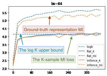
Figure 1: FlatNCE continues to robustly optimize the ground-truth MI for representation even after the finite sample loss has saturated at $\log K$.

We believe addressing ($ii$) and ($iii$) holds the key to resolving ($i$). A major inconsistency between theory and practice is that, contrary to expectation, more biased estimators such as InfoNCE work better in practice than their tighter counterparts [31]. The prevailing conjecture is that these biased contrastive learners benefit from a lower estimation variance [21, 32]. However, this conjecture is mostly based on experimental observations rather than formal variance analyses [33], and the comparison is not technically fair since the less biased estimators use far less samples [13, 34, 3]. Such incomplete understandings are partly caused by the absence of proper generic diagnostic tools to analyze contrastive learners. In this study, we hope to improve both the understanding and practice of contrastive representation learning via bridging these gaps.

Our development starts with two simple intuitions: ($i$) the contrasts between positive and negative data should be as large as possible, and ($ii$) the objective should be properly normalized to yield minimal variance. These heuristics lead to a simple, powerful, theoretically grounded novel contrastive learning objective we call FlatNCE. We show FlatNCE is the mathematical dual of InfoNCE [13], a widely used MI estimator that empowers models such as SimCLR [1], SimCSE [8], CLIP [9] and ALIGN [35]. What makes FlatNCE unique is that it has deep roots in statistical physics, which enables it to optimize beyond the finite-sample bottleneck that has plagued InfoNCE (Figure 1).

Importantly, our research brings new insights into contrastive learning. While the new energy perspective continues to reinforce the heuristic of contrastive learning, FlatNCE shows appealing to a cross-entropy-based predictive objective is suboptimal. This echoes recent attempts in building non-discriminative contrastive learners [22], and to the best of our knowledge, we provide the first of its kind that comes with rigorous theoretical guarantees. Further, FlatNCE inspires a set of diagnostic tools that will benefit the contrastive learning community as a whole [21].

2 Contrastive Representation Learning with InfoNCE

This section reviews the technical aspects of InfoNCE, how it is used to empower representation learning, and explains why InfoNCE fails in small-batch training, hence motivating our work.

2.1 InfoMax with noise contrastive estimation

Estimation of mutual information (MI) is central to many scientific investigations and engineering problems [36, 37, 38], thus motivating a plethora of practical procedures [39, 40, 41, 42, 43, 44, 45, 46]. Recently, burgeoning deep learning applications have raised particular interest in variational estimators of MI [13], for they usually deliver stable performance and are easily amendable to gradient-based optimization. Among the many variational MI estimators, InfoNCE stands out for its conceptual simplicity, ease of implementation and, crucially, strong empirical performance.

InfoNCE is a multi-sample mutual information estimator built on the idea of noise contrastive estimation (NCE) [47]. It was first described in [4] under the name contrastive predictive coding (CPC), and later formalized and coined InfoNCE in the work of [13]. Formally defined by

$$I_{\texttt{InfoNCE}}^{K}(X;Y|f)\triangleq\mathbb{E}_{p^{K}(x,y)}\left[\log\frac{f(x_{1},y_{1}^{\oplus})}{\frac{1}{K}\sum_{k^{\prime}}f(x_{1},y_{k^{\prime}}^{\ominus})}\right],I_{\texttt{InfoNCE}}^{K}(X;Y)\triangleq\underset{f\in\mathcal{F}}{\max}\{I_{\texttt{InfoNCE}}^{K}(X;Y|f)\},$$ (1)

InfoNCE implements the heuristic to discern positive samples from the negative samples, whereas the positives from the joint data distribution $p(x,y)$, and the negatives are randomly paired samples from respective marginal distributions $p(x)p(y)$. Here $f(x,y)>0$ is known as the critic function and we have used $p^{K}(x,y)$ to denote $K$ independent draws, which is the sample size or (mini) batch-size. Note we have used $\oplus$ and $\ominus$ to emphasize positive and negative samples. Mathematically, InfoNCE constructs a formal lower bound to the mutual information, given by the following statement:

Proposition 2.1.

InfoNCE is an asymptotically tight lower bound to the mutual information, i.e.,

$$I(X;Y)\geq I_{\texttt{InfoNCE}}^{K}(X;Y|f),\quad\lim_{K\rightarrow\infty}I_{\texttt{InfoNCE}}^{K}(X;Y)\rightarrow I(X;Y).$$ (2)

A few technical remarks are useful for our subsequent developments: ($i$) the $K$-sample InfoNCE estimator is upper bounded by $\log K$; ($ii$) in practice, InfoNCE is implemented with the CrossEntropy loss for multi-class classification, where $f(x,y)$ is parameterized by its logit $g_{\theta}(x,y)=\log f(x,y)$; ($iii$) optimizing for $f(x,y)$ tightens the bound, and the bound is sharp if $f(x,y)=p(x|y)e^{c(x)}$, where $c(x)$ is an arbitrary function on $\mathcal{X}$; and ($iv$) InfoNCE’s successes have been largely credited to the fact that its empirical estimator has much smaller variance relative to competing solutions. More details on these technical points are either expanded in later sections or deferred to the Appendix.

2.2 InfoNCE for contrastive representation learning

MI estimation is keenly connected to the literature on contrastive representation learning, with prominent examples such as Word2vec [15], MoCo [6], SimCLR [1], SimCSE [8], etc. In such works, one wants to build a robust feature extractor $\text{Enc}(x):\mathcal{X}\rightarrow\mathcal{Z}$ in an unsupervised way, such that the encoded representation $z=\text{Enc}(x)$ robustly encodes useful information in $x$ for various downstream applications. A general framework adopted by such works is that one first specifies a set of valid data augmentation transformations $\mathcal{T}\triangleq\{t:\mathcal{X}\rightarrow\mathcal{X}\}$ (e.g., for image data these transformations typically include crop, resize, flip, color distortion, cutout, noise corruption, blurring, filtering, etc.). Then, one tries to optimize for the heuristic goal that the encoded representation for the same data with different augmentations, sometimes referred to as different views [48], should still be more similar compared to those encoded from different data points (i.e., negative samples). Dot-product $\langle a,b\rangle=a^{T}b$ is often employed for efficient evaluation of similarity, and representations are typically normalized to unit spherical spaces (i.e., $\|z\|=1$) [49]. More specifically, let $t,t^{\prime}\in\mathcal{T}$ be two different transforms, these representation learning objectives optimize for different variants of the following cross-entropy-like loss

$$\ell(z,z_{\oplus}^{\prime},\{z_{\ominus,k}^{\prime}\}_{k=1}^{K})=-\log\frac{\exp(\beta\langle z,z_{\oplus}^{\prime}\rangle)}{\sum_{z^{\prime}\in\{\oplus,\ominus\}}\exp(\beta\langle z,z^{\prime}\rangle)},$$ (3)

where $z=\text{Enc}(t(x)),z_{\oplus}^{\prime}=\text{Enc}(t^{\prime}(x)),z_{\ominus,k}^{\prime}=\text{Enc}(t^{\prime}(x_{k}))$ for $x_{k}\neq x$, and $\beta>0$ is the inverse temperature parameter. Note (3) essentially tries to predict the positive sample out of the negative samples. One can readily recognize that (3) is mathematically equivalent to the InfoNCE target (1), up to a constant term $\log K$ and a much simplified bi-linear critic function $g(z,z^{\prime})=\beta\langle z,z^{\prime}\rangle$. This implies contrastive objectives are essentially optimizing for the mutual information $I(t(X);t^{\prime}(X))$ between different views of the data. Let $z=\text{Enc}(t(x))$ and $z^{\prime}=\text{Enc}(t^{\prime}(x))$, by the data processing inequality, we have $I(t(X);t^{\prime}(X))\geq I(Z;Z^{\prime})\geq I_{\texttt{InfoNCE}}(Z;Z^{\prime})$. A general observation made in the contrastive representation learning literature is that performance improves as $K$ gets larger, e.g., in SimCLR the performance grows with $K$ and reaches its optimum at $K=4,096$ with a ResNet50 architecture. These observations are consistent with our theoretical assertion that this MI bound gets tight as $K\rightarrow\infty$. However, this fact is challenging for budgeted applications and many investigators simply because training at such a scale is economically unaffordable.

2.3 The failure of InfoNCE with small batch-sizes

Despite InfoNCE’s sweeping successes, here we provide a careful analysis to expose its Achilles heel. Particularly, we reveal that as the InfoNCE estimate approaches saturation (i.e., $\hat{I}_{\texttt{InfoNCE}}\rightarrow\log K$, where $\hat{I}$ denotes an empirical sample estimate), its learning efficiency plunges due to limited numerical precision, hindering further improvements. This clarifies InfoNCE’s small-sample collapse and motivates our repairs in subsequent sections.

Recall in InfoNCE that the loss is computed from the CrossEntropy loss. For most deep learning platforms, the internal implementations exploit the stable logsumexp trick

$$\ell_{\text{CE}}=\texttt{logsumexp}(\{g_{ij}^{\ominus}\})-g_{ii}^{\oplus}=\{\log(\sum\nolimits_{j\in\{\oplus,\ominus\}}\exp(g_{ij}^{\ominus}-g_{\max}^{\ominus}))+g_{\max}^{\ominus}\}-g_{ii}^{\oplus},$$ (4)

to avoid numerical overflow, where $g_{ij}\triangleq g_{\theta}(x_{i},y_{j})$. With a powerful learner for $g_{\theta}(x,y)$ and a small $K$ such that $I(X;Y)>\log K$, we can reasonably expect $\hat{I}_{\texttt{InfoNCE}}\approx\log K$ after a few training epochs. Since $g_{ii}^{\oplus}$ itself is also included in the negative samples, this implies $g_{ii}^{\oplus}\gg g_{ij}^{\ominus},\,\,\forall j\neq i$ almost always holds true, because $\hat{I}_{\texttt{InfoNCE}}=\log\frac{\exp(g_{ii}^{\oplus})}{\frac{1}{K}\sum_{j}\exp(g_{ij}^{\ominus})}\approx\log\frac{\exp(g_{ii}^{\oplus})}{\frac{1}{K}\exp(g_{ii}^{\oplus})}=\log K$. So the contrast now becomes

$$\ell_{\text{CE}}=g_{ii}^{\oplus}+\log(\sum\nolimits_{j}\exp(g_{ij}^{\ominus}-g_{ii}^{\oplus}))-g_{ii}^{\oplus}=g_{ii}^{\oplus}+\log(1+o(1))-g_{ii}^{\oplus}\approx 0.$$ (5)

This is where the algorithm becomes problematic: for low-precision floating-point arithmetic, e.g., float32 or float16 as in standard deep learning applications, the relative error is large when two similar numbers are subtracted from one another. The contrastive terms $g_{ij}^{\ominus}-g_{ii}^{\oplus}$, which are actually contributing the learning signals, will be engulfed by the dominating $g_{ii}^{\oplus}$ and accumulate rounding errors. For an easy fix, one can explicitly modify the computation graph to cancel out $g_{ii}^{\oplus}$, as the CrossEntropy shipped with platforms such as Tensorflow and PyTorch does not do so.

3 FlatNCE And Generalized Contrastive Representation Learning

In this section, we deconstruct the building principles of contrastive learning to make fixes to the InfoNCE. Our new proposal, named FlatNCE, addresses the limitations of the naïve InfoNCE and comes with strong theoretical grounding. Detailed derivations are relegated to the Appendix.

Algorithm 1 FlatNCE

  Empirical data distribution $\hat{p}_{d}=\{(x_{i},y_{i})\}_{i=1}^{n}$

  for $t=1,2,\cdots$ do

     Sample $i,i_{k}^{\prime}\sim[1,\cdots,n],k^{\prime}\in[1,\cdots,K]$

     ${\boldsymbol{g}}_{\oplus}=g_{\theta}(x_{i},y_{i}),{\boldsymbol{g}}_{\ominus}=g_{\theta}(x_{i},y_{i_{k}^{\prime}})$

     # $\texttt{logits}=[{\boldsymbol{g}}_{\oplus},{\boldsymbol{g}}_{\ominus}],\texttt{labels}=\boldsymbol{0}$

     # $\ell_{\texttt{InfoNCE}}=\texttt{CrossEntropy}(\texttt{logits},\texttt{labels})$

     $\texttt{clogits}=\texttt{logsumexp}({\boldsymbol{g}}_{\ominus}-{\boldsymbol{g}}_{\oplus})$

     $\ell_{\texttt{FlatNCE}}=\exp(\texttt{clogits}-\texttt{detach}[\texttt{clogits}])$

     # Use your favorite optimizer

  end for

3.1 Making it flat: InfoNCE recasted

Recall in the InfoNCE objective the critic function $g_{\theta}(x,y)$ computes an affinity score for a pair of data $(x,y)$ and optimizes for the following intuition: paired $(x_{i},y_{i})$, known as the positives, should have larger affinity scores relative to the negative samples $\{(x_{i},y_{j})\}$, where $y_{j}$ is randomly drawn from the marginal distribution of $y$. For a good representation, where the InfoNCE estimation is maximized, we would like to make the affinity score contrasts $\Delta_{ij}\triangleq g_{\theta}(x_{i},y_{j})-g_{\theta}(x_{i},y_{i})$ as negative as possible. The challenge is to make negative contrasts continually improve after $I_{\texttt{InfoNCE}}$ has reached $\log K$.

So motivated, we drop the positive-sample prediction accuracy, and instead seek to directly optimize the affinity score contrasts to make them dip further after $I_{\texttt{InfoNCE}}$ has saturated. We begin with a discussion of the desirable properties for such an objective: ($i$) differential penalty and ($ii$) instance normalization. By differential penalty, we want the objective to nonlinearly regularize the affinity contrast, i.e., through the use of a link function $h(\Delta_{ij})$, such that it penalizes more heavily for smaller affinity differences, and has diminishing effect on affinity differences that are already sufficiently negative. Secondly, instance normalization attends to the fact that different $x$ may have different baselines for the affinity contrasts, which should be properly equalized. To see this, we recall in theory the optimal critic for InfoNCE is $g^{*}(x,y)=\log p(x|y)+c(x)$, so the expected value of $\mathbb{E}_{p(y^{\prime})}[g(x,y^{\prime})]$ varies with $x$, and it needs to be offset differently.

With these design principles in mind, now we start to build such a surrogate objective. Naturally, the tempered exponential transform $\exp(\beta t)$ meets our expectation for the link function, where $\beta>0$ is a tuning parameter known as the inverse temperature. To simplify our discussion, we always treat $\beta=1$ unless otherwise noted. On the other hand, incentivized by InfoNCE’s successes due to small estimating variance, we want the resulting objective to enjoy a low-variance profile. Taking this to the extreme, we propose FlatNCE, a zero-variance mini-batch MI optimizer, defined as

$$I_{\texttt{FlatNCE}}=\frac{\sum_{j}\exp(g_{\theta}(x_{i},y_{j}^{\prime})-g_{\theta}(x_{i},y_{i}))}{\texttt{detach}[\sum_{j^{\prime}}\exp(g_{\theta}(x_{i},y_{j^{\prime}}^{\prime})-g_{\theta}(x_{i},y_{i}))]},$$ (6)

where detach[$f_{\theta}(x)$] is an operation that bars gradient back-propagation. In accordance with the notation employed by InfoNCE, $j\in\{1,\cdots,K-1\}$ indexes the $K-1$ negative samples drawn from $p_{d}(y)$, so together with the positive sample (6) gives a $K$-sample estimator. One may readily notice that this is a flat function, as $I_{\texttt{FlatNCE}}\equiv 1$ for arbitrary inputs, which fulfills the zero-variance property. In this regard, we consider FlatNCE as a self-normalized contrastive objective. In the next section, we rigorously prove how FlatNCE is formally connected to InfoNCE, and why it is more preferable as confirmed by our experiments in Section 5.

3.2 Understanding FlatNCE

We first define the following variant of the FlatNCE

$$I_{\texttt{FlatNCE}}^{\oplus}(g_{\theta})=\frac{1+\sum_{j}\exp(g_{\theta}(x_{i},y_{j}^{\prime})-g_{\theta}(x_{i},y_{i}))}{1+\texttt{detach}[\sum_{j^{\prime}}\exp(g_{\theta}(x_{i},y_{j^{\prime}}^{\prime})-g_{\theta}(x_{i},y_{i}))]}.$$ (7)

Note that $I_{\texttt{FlatNCE}}^{\oplus}(g_{\theta})$ corresponds to adding the positive sample $y_{i}$ to the set of negative samples, because the zero contrast of the positive sample always gives the constant one. The following statement verifies $I_{\texttt{FlatNCE}}^{\oplus}(g_{\theta})$ is equivalent to InfoNCE in terms of differentiable optimization.

Proposition 3.1.

$\nabla_{\theta}I_{\texttt{FlatNCE}}^{\oplus}(g_{\theta})=\nabla_{\theta}I_{\texttt{InfoNCE}}(g_{\theta})$.

Equation (7) and Proposition 3.1 indicate how InfoNCE and FlatNCE are connected. Based on this, we can continue our discussion in Section 2.3 on why InfoNCE fails for small batch sizes. We start by showing the gradient of FlatNCE and its variant $I_{\texttt{FlatNCE}}^{\oplus}$ (so equivalently, InfoNCE) is given by a self-normalized importance-weighted gradient estimator, as formalized below.

Proposition 3.2.

The gradient of FlatNCE is an importance-weighted estimator of the form

$$\nabla I_{\texttt{FlatNCE}}=\sum\nolimits_{j}w_{j}\nabla g_{\theta}(x_{i},y_{j})-\nabla g_{\theta}(x_{i},y_{i}),\quad\text{ where }w_{j}=\frac{\exp(g_{\theta}(x_{i},y_{j}^{\prime}))}{\sum_{j^{\prime}}\exp(g_{\theta}(x_{i},y_{j^{\prime}}^{\prime})))}.$$ (8)

Without loss of generality, let us denote $y_{0}^{\prime}=y_{i}$, so when $\hat{I}_{\texttt{InfoNCE}}$ approaches $\log K$, we know $w_{0}\approx 1,w_{j>0}\approx 0$, and consequently $\nabla I_{\texttt{InfoNCE}}\approx\nabla g_{\theta}(x_{i},y_{i})-\nabla g_{\theta}(x_{i},y_{i})=0$. Consequently, as long as the positive sample is in the denominator the learning signal vanishes. What makes matters worse, the low-precision computations employed to speed up training introduce rounding errors, further corrupting the already weak gradient. On the other hand, in FlatNCE larger weights will be assigned to the more challenging negative samples in the batch, thus prioritizing hard negatives.

Proposition 3.2 also sheds insights on temperature annealing. Setting $\beta\neq 1$ re-normalizes the weights by exponential scaling (i.e., $w_{j}(\beta)=w_{j}^{\beta}/\sum_{j^{\prime}}w_{j^{\prime}}^{\beta}$). So the optimizer will focus more on the hard negative samples at a lower temperature (i.e., larger $\beta$), while for a higher temperature it treats all negative samples more equally. This new gradient interpretation reveals that $\beta$ affects the learning dynamics in addition to the well-known fact that $\beta$ modulates MI bound tightness.

Lastly, to fill in an important missing piece, we prove that FlatNCE is a formal MI lower bound.

Lemma 3.3.

For $\{(x_{j},y_{j})\}_{j=1}^{K}$, let $I_{\texttt{InfoNCE}}^{K}(g_{\theta})\triangleq-\log\frac{1}{K}\sum_{j}\exp(g_{\theta}(x_{1},y_{j}^{\ominus})-g_{\theta}(x_{1},y_{1}^{\oplus}))$. Then for arbitrary $u\in\mathbb{R}$, we have inequality

$$I_{\texttt{InfoNCE}}^{K}(g_{\theta})\geq 1-u-\frac{1}{K}\sum\nolimits_{j}\exp(-u+g_{\theta}(x_{1},y_{j})-g_{\theta}(x_{1},y_{1})),$$ (9)

and the equality holds when $u=\frac{1}{K}\sum_{j}\exp(g_{\theta}(x_{1},y_{j})-g_{\theta}(x_{1},y_{1}))$.

What makes this particularly interesting is that FlatNCE can be considered the conjugate dual of InfoNCE. In convex analysis, $u$ and $g$ in (9) are known as the Fenchel conjugate pair [50, 51, 52]. By taking the expectation wrt $p^{K}(x,y)$ and setting $u(\{(x_{j},y_{j})\})$ to its optimal value, we essentially recover $I_{\texttt{FlatNCE}}^{\oplus}(g_{\theta})$: the only difference to the conjugate of InfoNCE is the term $(1-u)$ which is considered fixed and does not participate in optimization. As such, the following Corollary is immediate.

Corollary 3.4.

$I_{\texttt{FlatNCE}}^{\oplus,K}(g_{\theta})=I_{\texttt{InfoNCE}}^{K}(g_{\theta})\leq I(X;Y),\,\,\,I_{\texttt{FlatNCE}}^{K}(g_{\theta})\leq I(X;Y)$.

3.3 Generalizing FlatNCE

The formulation of FlatNCE enables new possibilities for extending contrastive representation learning beyond its original form. In this section, we discuss some generalizations that make contrastive learning more flexible, including new tools for training diagnosis and tuning.

Effective sample-size (ESS) scheduling. While existing contrastive training schemes view temperature parameter $\beta$ as a static hyper-parameter that tunes model performance, our Proposition 3.2 shows that it also plays a dynamic role in updating the critic $g_{\theta}(x,y)$. This motivates us to anneal the contrastive learning by scheduling the temperature parameter. To exact better control over the training process through $\beta$, we appeal to the notation of normalized effective sample-size (ESS), defined by

$$\text{ESS}\triangleq 1/\{K\sum\nolimits_{j}w_{j}^{2}\}\in[1/K,1].$$ (10)

ESS provides richer information about the training than the estimated MI. A value close to $\text{ESS}\approx 1$ implies gradient diversity, as all samples are contributing to the gradient equally; $\text{ESS}\approx 0$ raises concern, as a small fraction of samples dominate the gradient, thus leading to a higher variance and consequently unstable training, as in the case of InfoNCE. So rather than directly employing temperature scheduling, we can instead instruct the model to train with the targeted level of ESS at each stage of training, namely ESS scheduling, which adaptively adjusts the temperature for the current model (see Algorithm S1 in Appendix). In early training it is more beneficial to aim at a higher ESS, such that model can more efficiently assimilate knowledge from a larger sample pool. As training progresses we gradually relax ESS constraints to allow the model to reach tighter MI bounds, while making sure gradient variance are kept under control.

Hölder FlatNCE. To further generalize contrastive learning, we re-examine the objective of FlatNCE. A key observation is that the numerator aggregates individual evidence of MI from the negative samples $(x,y^{\prime})\sim p(x)p(y^{\prime})$ through the critic function $g_{\theta}(x,y)$, with arithmetic mean. Possibilities are that if we change the aggregation step, we also change how it learns MI in a way similar to the importance weighting perspective discussed above. This inspires us to consider the more general aggregation procedures, such as the Hölder mean defined below.

Definition 3.5 (Hölder mean).

For $\{a_{i}\in\mathbb{R}_{+}\}_{i=1^{n}}$ and $\gamma\in\mathbb{R}$, the Hölder mean is defined as $m_{\gamma}(\{a_{i}\}_{i=1}^{n})=\left(\frac{1}{n}\sum_{i}a_{i}^{\gamma}\right)^{\frac{1}{\gamma}}$.

Note Hölder mean recovers many common information pooling operations, such as $\min$ ($\gamma=-\infty$), $\max$ ($\gamma=\infty$), geometric mean ($\gamma\rightarrow 0$), root mean square ($\gamma=2$), and arithmetic mean ($\gamma=1$) as employed in our FlatNCE. This allows us to define a new family of contrastive learning objectives.

Definition 3.6 (Hölder-FlatNCE).

$I_{\gamma}\triangleq\sum_{i}\frac{m_{\gamma}(\{\exp(g_{ij}^{\ominus}-g_{ii}^{\oplus})\}_{j})}{\texttt{detach}[m_{\gamma}(\{\exp(g_{ij}^{\ominus}-g_{ii}^{\oplus})\}_{j})]}$.

The following Proposition shows that Hölder-FlatNCE is equivalent to annealed FlatNCE.

Proposition 3.7.

$\nabla I_{\gamma}(g_{\theta})=\nabla I_{\texttt{FlatNCE}}(\gamma\cdot g_{\theta})$.

As an important remark, we note the sample gradient of FlatNCE is a (randomly) re-scaled copy of the true gradient (normalized by $Z_{\theta}$ instead of $\hat{Z}_{\theta}$), so we are still optimizing the model in the right direction using stochastic gradient descent (SGD) [53]. This property can be used to ascertain the algorithmic convergence of FlatNCE, formalized in the Proposition below. Details in Appendix.

Proposition 3.8 (Convergence of FlatNCE, simple version).

Under the technical conditions in Assumption A1, with Algorithm 1 $\theta_{t}$ converges in probability to a stationary point of the unnormalized mutual information estimator $I(\theta)\triangleq\mathbb{E}_{p(x,y)}[g_{\theta}(x,y)]-\mathbb{E}_{p(x)}[\log Z_{\theta}(x)]$ (i.e., $\lim_{t\rightarrow\infty}\|\nabla I(g_{\theta_{t}})\|=0$), where $Z_{\theta}(x)\triangleq\mathbb{E}_{p(y)}[e^{g_{\theta}(x,y)}]$. Further assume $I(\theta)$ is convex with respect to $\theta$, then $\theta_{t}$ converges in probability to the global optimum $\theta^{*}$ of $I(\theta)$.

4 Rethinking Contrastive Learning: Experimental Evidence & Discussions

Figure 2: Sample efficiency comparison for SimCLR and FlatCLR on Cifar10.

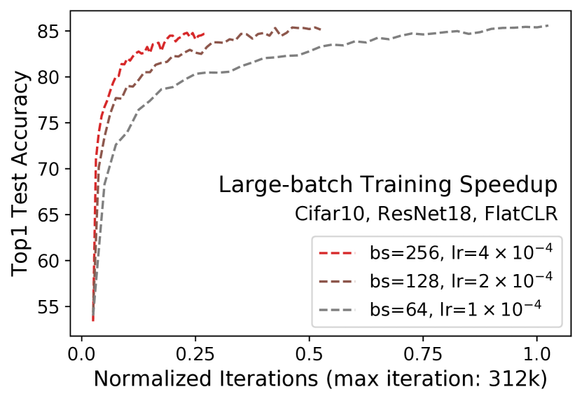
Figure 3: Speed up of large-batch training. Larger batch leads to faster convergence.

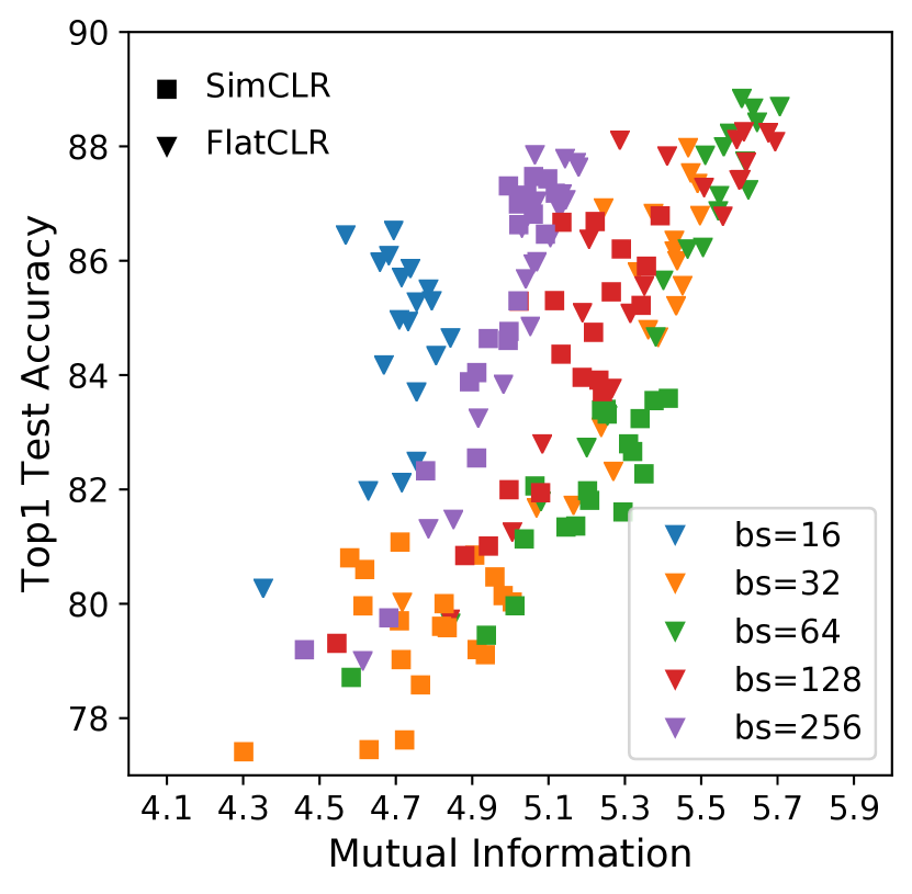
Figure 4: Representation MI strongly correlates with performance.

We contribute this section to the active discussions on some of the most important topics in contrastive learning. Our discussions will be grounded on the new experimental results from Cifar10 with a ResNet backbone, with a PyTorch codebase of the InfoNCE-backed SimCLR and its FlatNCE counterpart FlatCLR. Note instead of trying to set new performance records (because of limited computational resources in our university setting), experiments in this section are designed to reveal important aspects of contrastive learning, and to ensure our results can be easily reproduced with reasonable computation resources. Details of our setups are elaborated on in Section 5.

Breaking the curse, small-batch contrastive learning revived. We show that with our novel FlatNCE objective, successful contrastive learning applications are no longer exclusive to the costly large-batch training. In Figure 4 we see pronounced small-sample performance degradation for SimCLR, while the FlatCLR is far less sensitive to the choice of batch size. In fact, we see FlatCLR-$16$ matches performance of its SimCLR-$128$ counterpart, corresponding to an $8\times$ boost in efficiency. And in all cases FlatCLR consistently works better compared to the same-batch-size SimCLR. Despite the encouraging improvements in the small-batch regime, large-batch training does provide better results for both SimCLR and FlatCLR. Additionally, leveling up parallelism greatly reduces the overall training time (Figure 4), as a larger batch-size enables stable training with a larger learning rate [54, 55, 56] . The main merits of our result are: ($i$) the enabling of contrastive learning for very budgeted applications, where large-batch learning is prohibitive; and ($ii$) consistent improvement over InfoNCE, especially wrt the cost-performance trade-off.

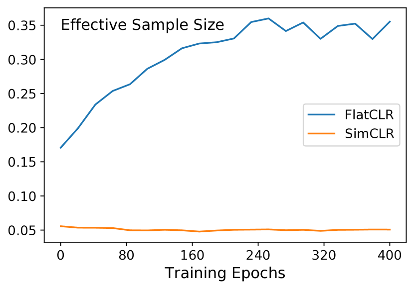
Figure 5: Effective sample size (c.f. Figure 1).

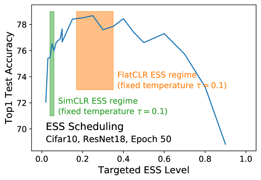
Figure 6: ESS scheduling results.

Is tighter MI bound actually better or worse? An interesting observation made by a few independent studies is that, perhaps contrary to expectation, tighter bounds on MI do not necessarily lead to better performance on the downstream tasks [31]. To explain this, existing hypotheses have focused on the variance and sample complexity perspectives [32]. To address this, we compare the actual MI to the mini-batch MI estimate, and plot the respective typical training curves in Figure 1. Since FlatNCE itself is not associated with a number to bound MI (because it is theoretically tight), we use an InfoNCE estimate based-on the FlatNCE representation. Observe that although the sample MI estimates are tied, FlatCLR robustly improves the ground-truth MI as SimCLR approaches the $\log$-$K$ saturation point and become stagnant. To further understand how MI relates to downstream performance, we plot the Top-$1$ accuracy against the true MI using all our model training checkpoints (Figure 4), and confirm a strong linear relation between the two (Pearson correlation $\rho=0.65$, $p$-value $<10^{-20}$). However, this link is not evident using the mini-batch sample MI (Figure S1 in Appendix).

ESS for monitoring and tuning contrastive learning. As an important tool introduced in this work, we want to demonstrate the usefulness of ESS in contrastive training. Figure 6 plots ESS curves for the training dynamics described in Figure 1, and we see drastically different profiles. As predicted by our analyses, SimCLR’s ESS monotonically decreases as it approaches the InfoNCE saturation (from $0.06$ to $0.05$), while FlatNCE-ESS instead climbs up ($0.17\rightarrow 0.35$). The performance gap widens as the ESS difference becomes larger, thus confirming the superior sample efficiency of FlatNCE. Next we experimented with ESS-scheduling: instead of a fixed temperature, we fix the ESS throughout training, and then compare model performance. Figure 6 shows a snapshot of training progress per targeted ESS value at epoch $50$, where the estimated MI just started to plateau. The result indicates ESS range $[0.15,0.4]$ works well for Cifar10, while SimCLR with fixed temperature only covers the sub-optimal $[0.04,0.06]$. These interesting observation warrant further future investigations on ESS control in contrastive training.

Self-normalized contrastive learning as constrained optimization. Here we want to promote a new view, which considers self-normalized contrastive learning as a form of constrained optimization. In this view, including multiple negative samples in the update of the critic function is necessary for contrastive learning. This conclusion comes from our numerous failed attempts in designing alternative few-sample contrastive learning objectives that simultaneously reduce estimation variance and tighten the MI bound (see Appendix for a detailed summary of our negative experience). Since the feature encoders are usually built with complex neural networks, the representations can be rather sensitive to the changes in encoder parameters. So while the gradient update direction may maximally benefit the MI estimate, it may disrupt the representation and thus compromise the validity of the variational MI estimate. Including negative samples in the updates of the critic $g_{\theta}$ allows the use of negative samples to provide instant feedback on which directions are bad, and to steer away from. More negative samples (i.e., a larger $K$) will enforce a more confined search space, thus allowing the critic updates to proceed more confidently with larger learning rates. Also, comparison should be made to importance-weighted variational auto-encoder (IW-VAE) [57], which also leverages a self-normalized objective for representation learning and inference. However, IW-VAE has been proven harmful to representation learning, although it provably tightens the likelihood bound [58]. Finally, our new approach also promises to scale up & improve generalized contrastive learning [59].

Table 1: Comparison of representative variational MI objectives. We use $(x,p_{\oplus})$ to denote the positive sample drawn from the joint density $p(x,y)$, $(x,y_{\ominus})$ for the negative samples from $p(x)p(y)$, and $m(x,y^{1:K})\triangleq\frac{1}{K}\sum_{k=1}^{K}\exp(g(x,y^{k}))$. See Appendix for more details.

Name	Objective	Bias	Stability
Donsker-Varadhan [60]	$g(x,y_{\oplus})-\log(\sum_{k=1}^{K}\exp(g(x^{k},y_{\ominus}^{k}))/K)$	Large	Poor
Nguyen-Wainwright-Jordan [61]	$g(x,y_{\oplus})-\sum_{k=1}^{K}\exp(g(x,y_{\ominus}^{k})-1)/K$	Low	Okay
Fenchel-Legendre [52]	$u(x,y_{\oplus})+\sum_{k=1}^{K}\exp(-u(x,y_{\oplus})+g(x,y_{\ominus})-g(x,y_{\oplus}))/K$	Low	Okay
InfoNCE [4]	$g(x,y_{\oplus})-\log(m(x,\{y_{\oplus},y_{\ominus}^{1:K-1}\}))$	Large	Excellent
FlatNCE (Ours)	$\{m(x,y_{\ominus}^{1:K})-g(x,y_{\oplus})\}/\texttt{detach}[\{m(x,y_{\ominus}^{1:K})-g(x,y_{\oplus}\}]$	Low	Excellent

Connections to variational mutual information estimation. Table 1 summarizes representative examples of nonparametric variational MI bounds in the literature, whose difference can be understood based on how information from negative samples are aggregated. Before InfoNCE, Donsker-Varadhan (DV) [60] and Nguyen-Wainwright-Jordan (NWJ) [61] are the most widely practiced MI estimators. NWJ is generally considered non-contrastive as positive and negative samples are compared, respectively, at $\log$ and $\exp$ scales. DV differs from InfoNCE by excluding the positive sample from the negative pool, which is similar to the practice of our FlatNCE. However, DV is numerically unstable and necessitates careful treatment to be useful [44]. Also note some literature had unfairly compared the the multi-sample InfoNCE to the single-sample versions of its competitors, partly because the alternatives do not have efficient multi-sample implementations. To the best of our knowledge, closest to this research is the concurrent work of [52], where the contrastive Fenchel-Lengendre estimator is derived. While developed independently from completely different perspectives, FlatNCE enjoys the duality view promoted by [52] and inherits all its appealing theoretical properties. Our theoretical and empirical results complemented nicely the theories from [52].

5 Further Experiments

The above discussion presented several experimental results to highlight unique aspects of the proposed approach. We now consider additional experiments to further validate the proposed FlatNCE and benchmark it against state-of-the-art solutions. We sketch our setup here and leave details to the Appendix. Our code can be assessed from https://github.com/Junya-Chen/FlatCLR. All experiments are implemented with PyTorch and executed on NVIDIA V100 GPUs with a maximal level of parallelism at 4 GPUs.

Self-supervised learning (SSL) on Cifar and ImageNet. We set our main theme in SSL and compare the effectiveness of the SimCLR framework [1] to our FlatNCE-powered FlatCLR. Our codebase is modified from a public PyTorch implementation. Specifically, we train $256$-dimensional feature representations by maximizing the self-MI between two random views of data, and report the test set classification accuracy using a linear classifier trained to convergence. We report performance based on ResNet-50, and some of the learning dynamics analyses are based on ResNet-18 for reasons of memory constraints. Hyper-parameters are adapted from the original SimCLR paper. For the large-batch scaling experiment, we first grid-search the best learning rate for the base batch-size, then grow the learning rate linearly with batch-size.

Table 2: ImageNet SSL results.

Epoch	10	20	30	40	50	60	70	80	90	100
SimCLR	38.57	43.71	47.03	49.45	49.93	52.18	53.31	53.47	53.98	54.62
FlatCLR	39.7	45.30	47.74	49.72	50.39	53.30	54.48	54.43	56.25	56.74

The observations made on Cifar align with our theoretical prediction (see Figure 4): in the early training (less than $50$ epochs), where the contrast between positives and negatives have not saturated, all models performed similarly. After that, performance start to diverge when entering a regime where FlatNCE learns more efficiently. See Section 4 and Appendix for more results and discussions.

Table 3: ImageNet SSL transfer learning results.

Dataset	Cifar10	Cifar100	VOC2007	Flower	Caltech101	SUN397
SimCLR	87.74	65.40	69.38	90.03	79.54	49.62
FlatCLR	87.92	65.76	69.66	90.23	81.23	51.31

We further apply our model to the ImageNet dataset and compare its performance to the SimCLR baseline. We note the SOTA results reported by [1] heavily rely on intensive automated hyper-parameter grid search, and considerably larger networks (i.e., ResNet50 $\times 4$ versus ResNet50), that we are unable to match given our (university-based) computational resources. So instead, we report fair comparison to the best of our affordability. Table 2 reports SSL classification performance comparison up to the $100$ epoch. In Table 3 we examine the performance of representation transfer to other datasets. For both cases, FlatCLR consistently outperforms the vanilla SimCLR.

6 Conclusions

We have presented a novel contrastive learning objective called FlatNCE, that is easy to implement, but delivers strong performance and faster model training. We show that underneath its simple expression, FlatNCE has a solid mathematical grounding, and consistently outperforms its InfoNCE counterpart for the experimental setting we considered. In future work, we seek to verify the effectiveness of FlatNCE on a computation scale not feasible to this study, and apply it to new architectures and applications. Also, we invite the community to find ways to reconcile the performance gap between those theoretically optimal MI bounds and those self-normalized sub-optimal bounds such as FlatNCE and InfoNCE, and develop principled theories for hard-negative training.

Appendix

Appendix A The Staggering Cost of Training Contrastive Learners

In Table S1 we summarize the associated cost of training state-of-the-art contrastive learners. We have used the numbers from the original papers to compute the cost. The number of devices and time of training for the largest model reported in the respective papers are used, while we use the online quotes from Google Cloud (for TPU units) and Amazon AWS (for GPU units) for the hourly cost of dedicated computing devices. We only focused on the computation cost, so the potential charges from storage and network traffic are omitted. Note that this table only reports the number of computing devices used in the final training where all parameters have been tuned to optimal, the actual expenditures associated with the development of these models can be significantly higher. Usually researchers and engineers spent more time tuning the parameters and exploring ideas before finally come up with a model that can be publicized. Also, the cost for performance evaluation is not count towards the cost, and some of the papers have employed intensive grid-search of parameters for evaluation, which in our experience can be even more costly than training the contrastive learners at times. And we do find fine-tuning evaluation can drastically boost the performance metrics.

Table S1: Cost of training a contrastive learner

Model	Sponsor	Neg. Size	Infrastructure	Train Time	Est. Cost
MoCo [6]	Facebook	$65,536$	$64$ V100 GPUs	$6$ days	$23k
SimCLR [1]	Google	$4,096$	$128$-core TPU-v3	$15$ hours	$1,720
CLIP [9]	OpenAI	$32,768$	$592$ V100 GPUs	$18$ days	$634k

Appendix B Technical Proofs

B.1 Proof of Proposition 2.1

Proof.

See [13] for a neat proof on how the multi-sample NWJ upper bounds InfoNCE. Since NWJ is a lower bound to MI, InfoNCE also lower bounds MI.

What remains is to show the InfoNCE bound is asymptotically tight. We only need to prove that with a specific choice of $f(x,y)$, InfoNCE recovers $I(X;Y)$. To this end, let us set $f(x,y)=f^{*}(x,y)=\frac{p(y|x)}{p(y)}$, and we have

$$I_{\texttt{InfoNCE}}^{K}(f^{*}) = \mathbb{E}_{p^{K}}\left[\log\left(\frac{f^{*}(x_{k},y_{k})}{f^{*}(x_{k},y_{k})+\sum_{k^{\prime}\neq k}f^{*}(x_{k},y_{k^{\prime}})}\right)\right]+\log K$$ (11)

$$= -\mathbb{E}\left[\log\left(1+\frac{p(y)}{p(y|x)}\sum_{k^{\prime}}\frac{p(y_{k^{\prime}}|x_{k})}{p(y_{k^{\prime}})}\right)\right]+\log K$$ (12)

$$\approx -\mathbb{E}\left[\log\left(1+\frac{p(y)}{p(y|x)}(K-1)\mathbb{E}_{y_{k^{\prime}}}\frac{p(y_{k^{\prime}}|x_{k})}{p(y_{k^{\prime}})}\right)\right]+\log K$$ (13)

$$= -\mathbb{E}\left[\log\left(1+\frac{p(y_{k})}{p(y_{k}|x_{k})}(K-1)\right)\right]+\log K$$ (14)

$$\approx \underbrace{-\mathbb{E}\left[\log\frac{p(y)}{p(y|x)}\right]}_{I(X;Y)}-\log(K-1)+\log K$$ (15)

Now taking $K\rightarrow\infty$, the last two terms cancels out. ∎

B.2 Proof of Proposition 3.1

Proof.

Without loss of generality we denote $y_{0}$ as the positive sample and all $y_{j},j>0$ as the negative samples. Recall

$$\texttt{CrossEntropyLoss}(\texttt{logits}=g_{\theta}(x_{0},y_{j}),\texttt{label}=0)$$ (17)

$$= -\log\frac{\exp(g_{\theta}(x_{0},y_{0}))}{\sum_{j}\exp(g_{\theta}(x,y_{j}))}$$ (18)

$$= \log\sum\nolimits_{j}\exp(g_{\theta}(x_{0},y_{j})-g_{\theta}(x_{0},y_{0}))$$ (19)

Since $\nabla\log f=\frac{\nabla f}{f}$, so

$$\nabla_{\theta}I_{\texttt{FlatNCE}}^{\oplus}(g_{\theta})=\nabla_{\theta}\mathcal{L}_{\texttt{CrossEntropy}}=\frac{\nabla_{\theta}\{\sum\nolimits_{j}\exp(g_{\theta}(x_{0},y_{j})-g_{\theta}(x_{0},y_{0}))\}}{\sum\nolimits_{j}\exp(g_{\theta}(x_{0},y_{j})-g_{\theta}(x_{0},y_{0}))}=\nabla_{\theta}I_{\texttt{InfoNCE}}(g_{\theta})$$ (20)

which concludes our proof (we omit the sign here for brevity). ∎

B.3 Proof of Proposition 3.2

Proof.

Let us pick up from (20) from last proof, we have

$$\nabla I_{\texttt{FlatNCE}} = \frac{\nabla_{\theta}\{\sum\nolimits_{j}\exp(g_{\theta}(x_{0},y_{j})-g_{\theta}(x_{0},y_{0}))\}}{\sum\nolimits_{j}\exp(g_{\theta}(x_{0},y_{j})-g_{\theta}(x_{0},y_{0}))}$$ (21)

$$= \frac{\sum\nolimits_{j}\exp(g_{\theta}(x_{0},y_{j})-g_{\theta}(x_{0},y_{0}))(\nabla_{\theta}\{g_{\theta}(x_{0},y_{j})-g_{\theta}(x_{0},y_{0})\})}{\sum\nolimits_{j}\exp(g_{\theta}(x_{0},y_{j})-g_{\theta}(x_{0},y_{0}))}$$ (22)

$$= \sum\nolimits_{j}w_{j}\nabla_{\theta}g_{\theta}(x_{0},y_{j})-(\sum\nolimits_{j}w_{j})\nabla_{\theta}g_{\theta}(x_{0},y_{0})$$ (23)

$$= \sum\nolimits_{j}w_{j}\nabla_{\theta}g_{\theta}(x_{0},y_{j})-g_{\theta}(x_{0},y_{0})$$ (24)

here $w_{j}\triangleq\exp(g_{\theta}(x_{0},y_{j}))/(\sum\nolimits_{j^{\prime}}\exp(g_{\theta}(x_{0},y_{j^{\prime}})))$, as the term $\exp(-g_{\theta}(x_{0},y_{0}))$ has been canceled out. ∎

B.4 Proof of Lemma 3.3

Our proof is inspired by the technique used in [51] for non-parametric likelihood approximations, which is based on the celebrated Fenchel-Legendre duality given below.

Definition S1 (Fenchel-Legendre duality [50]).

Let $f(t)$ be a proper convex, lower-semicontinuous function; then its convex conjugate function $f^{*}(v)$ is defined as $f^{*}(v)=\sup_{t\in\mathcal{D}(f)}\{tv-f(t)\}$, where $\mathcal{D}(f)$ denotes the domain of function $f$ [62]. We call $f^{*}(v)$ the Fenchel-Legendre conjugate of $f(t)$, which is again convex and lower-semicontinuous. The Fenchel-Legendre conjugate pair $(f,f^{*})$ are dual to each other, in the sense that $f^{**}=f$, i.e., $f(t)=\sup_{v\in\mathcal{D}(f^{*})}\{vt-f^{*}(v)\}.$

Example. The Fenchel-Legendre dual for $f(t)=-\log(t)$ is $f^{*}(v)=-1-\log(-v)$.

Proof of Lemma 3.3.
Let us write InfoNCE as

$$I_{\texttt{InfoNCE}}(g)=-\log\sum\nolimits_{j}\exp(g_{\theta}(x_{0},y_{j})-g_{\theta}(x_{0},y_{0})).$$ (25)

Replacing the $-\log(t)$ term in $I_{\texttt{InfoNCE}}(t)$ with its Fenchel-Legendre dual $-1-\log(-v)$, then Proposition is immediate after properly rearranging the terms and write $u=-\log v$. $\square$

B.5 Proof of Corollary 3.4

To make our proof simpler, we follow some theoretical results developed in [52], included below for completeness.

Proposition S2 (The Fenchel-Legendre Optimization Bound, Proposition 2.2 in [52]).

$$I_{\texttt{FLO}}(u,g)\triangleq\left\{\mathbb{E}_{p(x,y)p(y^{\prime})}\left[u(X,Y)+\exp(-u(X,Y)+g(X,Y^{\prime})-g(X,Y))\right]\right\}+1$$ (26)

$$I(X;Y)=-\min_{u,g}\{I_{\texttt{FLO}}(u,g)\}$$ (27)

Sketch of proof for Proposition S2. Recall the Donsker-Varadhan (DV) bound [60] is given by

$$I_{\texttt{DV}}\triangleq\mathbb{E}_{p(x,y)}[g(x,y)-\log(\mathbb{E}_{p(y^{\prime})}[\exp(g(x,y^{\prime}))])].$$ (28)

Then we proceed similarly to the proof of Lemma 3.3.

Remark. Here we consider $g(x,y)$ as the primal critic and $u(x,y)$ as the dual critic. Since arbitrary choice of primal/dual critics always lower bounds MI, we can either jointly optimize the two critics, or train in an iterative fashion: optimize one at a time while keep the other fixed. Let us consider the case $u$ is fixed and only update $g$, the proof below shows with an appropriate choice of $u$, Corollary 3.4 follows.

Proof of Corollary 3.4
Given $g_{\theta}(x,y)$ and empirical samples $\{(x_{j},y_{j})\}$, let us set $u(x,y)$ to

$$\hat{u}^{*}(g_{\theta})=\log\left(\frac{1}{K}\sum\nolimits_{j}\exp(g_{\theta}(x_{i},y_{j})-g_{\theta}(x_{i},y_{i}))\right)$$ (29)

Plug $(g_{\theta},\hat{u}^{*})$ into the right hand side of Equation (9) proves $\hat{u}^{*}+I_{\texttt{FlatNCE}}-1$ lower bounds mutual information. Since $\hat{u}^{*}$ does not contribute gradient, we can consider $I_{\texttt{FlatNCE}}\leq I(X;Y)$ holds up to a constant term. In other words, we are effectively optimizing a lower bound to MI, although $I_{\texttt{FlatNCE}}$ does not technically a lower bound – this is still OK since the difference does not contribute learning signal. $\square$

B.6 Proof of Proposition 3.7

Proof.

Denoting $f_{j}=\exp(g_{j})$, and we have

$$\nabla I_{\gamma}(g_{\theta}) = \frac{\nabla m_{\gamma}(\{f_{j}\})}{m_{\gamma}(\{f_{j}\})}$$ (30)

$$= \frac{\frac{1}{\gamma}(\frac{1}{n}\sum_{j}f_{j}^{\gamma})^{\frac{1}{\gamma}-1}\{\gamma\frac{1}{n}\sum_{j}f_{j}^{\gamma-1}\nabla f_{j}\}}{(\frac{1}{n}\sum_{j}f_{j}^{\gamma})^{\frac{1}{\gamma}}}$$ (31)

$$= \frac{\sum_{j}f_{j}^{\gamma-1}\nabla f_{j}}{\sum_{j}f_{j}^{\gamma}}$$ (32)

$$= \frac{\nabla\sum_{j}\exp(\gamma g_{j})}{\gamma\sum_{j}\exp(\gamma g_{j})}$$ (33)

$$= \frac{1}{\gamma}\nabla I_{\texttt{FlatNCE}}(\gamma\cdot g_{\theta})$$ (34)

∎

B.7 Proof of Proposition 3.8

Here we detail the technical conditions for Proposition 3.8 to hold. Our derivation follows the analytic framework of generalized SGD from [51], included below for completeness.

Definition S3 (Generalized SGD, Problem 2.1 [51]).

Let $h(\theta;\omega),\omega\sim p(\omega)$ be an unbiased stochastic gradient estimator for objective $f(\theta)$, $\{\eta_{t}>0\}$ is the fixed learning rate schedule, $\{\xi_{t}>0\}$ is the random perturbations to the learning rate. We want to solve for $\nabla f(\theta)=0$ with the iterative scheme $\theta_{t+1}=\theta_{t}+\tilde{\eta}_{t}\,h(\theta_{t};\omega_{t}),$ where $\{\omega_{t}\}$ are iid draws and $\tilde{\eta}_{t}=\eta_{t}\xi_{t}$ is the randomized learning rate.

Assumption S4.

(Standard regularity conditions for SGD, Assumption D.1 [51]).

1. $h(\theta)\triangleq\mathbb{E}_{\omega}[h(\theta;\omega)]$ is Lipschitz continuous;

2. The ODE $\dot{\theta}=h(\theta)$ has a unique equilibrium point $\theta^{*}$, which is globally asymptotically stable;

3. The sequence $\{\theta_{t}\}$ is bounded with probability one;

4. The noise sequence $\{\omega_{t}\}$ is a martingale difference sequence;

5. For some finite constants $A$ and $B$ and some norm $\|\cdot\|$ on $\mathbb{R}^{d}$, $\mathbb{E}[\|\omega_{t}\|^{2}]\leq A+B\|\theta_{t}\|^{2}$ almost surely $\forall t\geq 1$.

Proposition S5 (Generalized SGD, Proposition 2.2 in [51]).

Under the standard regularity conditions listed in Assumption S4, we further assume $\sum_{t}\mathbb{E}[\tilde{\eta}_{t}]=\infty$ and $\sum_{t}\mathbb{E}[\tilde{\eta}_{t}^{2}]<\infty$. Then $\theta_{n}\rightarrow\theta^{*}$ with probability one from any initial point $\theta_{0}$.

Assumption S6.

(Weak regularity conditions for generalized SGD, Assumption G.1 in [51]).

1. The objective function $f(\theta)$ is second-order differentiable;

2. The objective function $f(\theta)$ has a Lipschitz-continuous gradient, i.e., there exists a constant $L$ satisfying $-LI\preceq\nabla^{2}f(\theta)\preceq LI$, where for semi-positive definite matrices $A$ and $B$, $A\preceq B$ means $v^{T}Av\leq v^{T}Bv$ for any $v\in\mathbb{R}^{d}$;

3. The noise has a bounded variance, i.e., there exists a constant $\sigma>0$ satisfying $\mathbb{E}\left[\left\|h(\theta_{t};\omega_{t})-\nabla f(\theta_{t})\right\|^{2}\right]\leq\sigma^{2}$.

Proposition S7 (Weak convergence, Proposition G.2 in [51]).

Under the technical conditions listed in Assumption S6, the SGD solution $\{\theta_{t}\}_{t>0}$ updated with generalized Robbins-Monro sequence ($\tilde{\eta}_{t}$: $\sum_{t}\mathbb{E}[\tilde{\eta}_{t}]=\infty$ and $\sum_{t}\mathbb{E}[\tilde{\eta}_{t}^{2}]<\infty$) converges to a stationary point of $f(\theta)$ with probability $1$ (equivalently, $\mathbb{E}\left[\|\nabla f(\theta_{t})\|^{2}\right]\rightarrow 0$ as $t\rightarrow\infty$).

Proof of Proposition 3.8.
For fixed $g_{\theta}(x,y)$ the corresponding optimal $u_{\theta}^{*}(x,y)$ maximizing the rhs in Equation (9) is given by

$$u_{\theta}^{*}(x,y)=\log\mathbb{E}_{p(y^{\prime})}[\exp(g_{\theta}(x,y^{\prime})-g_{\theta}(x,y))]\triangleq-\log\mathcal{E}_{\theta}(x,y),$$ (35)

so $\hat{\mathcal{E}}_{\theta}(x,y)\triangleq\exp^{-\hat{u}_{\phi}(x,y)}$ can be considered as approximations to $\mathcal{E}_{\theta}(x,y)$.

$$\nabla_{\theta}\{(9)\} = -\mathbb{E}_{p(x,y)}\left[e^{-u_{\phi}(x,y)}\mathbb{E}_{p(y^{\prime})}[\nabla_{\theta}\exp(g_{\theta}(x,y^{\prime})-g_{\theta}(x,y))]\right]$$ (36)

$$= \mathbb{E}_{p(x,y)}\left[\frac{\hat{\mathcal{E}}_{\theta}(x,y)}{\mathcal{E}_{\theta}(x,y)}\nabla_{\theta}\log\mathcal{E}_{\theta}(x,y)\right]$$ (37)

Note $I_{\texttt{BA}}\triangleq\max_{g_{\theta}}\{\mathbb{E}_{p(x,y)}[\log\mathcal{E}_{\theta}(x,y)]\}$ is the well-known Barber-Agakov (BA) representation of mutual information (i.e., $I_{\texttt{BA}}=I(X;Y)$) [63, 13], so optimizing Equation (9) with SGD is equivalent to optimize $I_{\texttt{BA}}$ with its gradient scaled (randomly) by $\hat{\mathcal{E}}_{\theta_{t}}/\mathcal{E}_{\theta_{t}}$ [52]. Under the additional assumption that $\hat{\mathcal{E}}_{\theta_{t}}/\mathcal{E}_{\theta_{t}}$ is bounded between $[a,b]$ ($0<a<b<\infty$), results follow by a direct application of Proposition S5 and Proposition S7. $\square$

Appendix C Algorithm for ESS Scheduling

We summarize the effective-sample size (ESS) scheduling scheme in Algorithm S1.

Algorithm S1 ESS Scheduling

  Empirical data distribution $\hat{p}_{d}=\{(x_{i},y_{i})\}_{i=1}^{n}$

  Inverse temperature $\beta=1$, ESS-scheduler $\{\varrho_{t}\in(1/K,1]\}_{t=1}^{T}$

  Adaptation rate $\gamma=0.01$

  for $t=1,2,\cdots,T$ do

     Sample $i,i_{k}^{\prime}\sim[1,\cdots,n],k^{\prime}\in[1,\cdots,K]$

     ${\boldsymbol{g}}_{\oplus}=g_{\theta}(x_{i},y_{i}),{\boldsymbol{g}}_{\ominus}=g_{\theta}(x_{i},y_{i_{k}^{\prime}})$

     $\texttt{clogits}=\texttt{logsumexp}({\boldsymbol{g}}_{\ominus}-{\boldsymbol{g}}_{\oplus})$

     $\texttt{weights}=\texttt{Softmax}({\boldsymbol{g}}_{\ominus}-{\boldsymbol{g}}_{\oplus})$

     $\texttt{ESS}=1./(K\cdot\texttt{square}(weights).sum())$

     $\ell_{\texttt{FlatNCE}}=\exp(\texttt{clogits}-\texttt{detach}[\texttt{clogits}])$

     # Use your favorite optimizer

     if $\texttt{ESS}>\varrho_{t}$ then

        $\beta=(1-\gamma)\cdot\beta$

     else

        $\beta=(1+\gamma)\cdot\beta$

     end if

  end for

Appendix D Failed Attempts to Overcome the $\log$-K Curse

The author(s) feel it is imperative to share not only successful stories, but more importantly, those failure experience when exploring new ideas. We contribute this section in the hope it will both help investigators avoid potential pitfalls and inspire new researches.

Joint optimization of primal-dual critics. Inspired by the concurrent research of [52], the author(s) of this paper had originally hope the joint optimization of primal-dual critic as defined in Equation (9) will match, and hopefully surpass the performance of multi-sample InfoNCE with single-sample estimation (i.e., $K=1$). The argument is follows: in theory, the single-sample Fenchel-Legendre estimator has the same expectation with its multi-sample variant, and is provably tighter than InfoNCE. In a sense, Fenchel-Legendre estimator is combining the gradient of FlatNCE and InfoNCE, and the potential synergy is appealing. Unfortunately, in our small scale trial experiments (i.e., MNIST and Cifar), we observe that while the Fenchel-Legendre estimator works reasonably well, it falls slightly below the performance of InfoNCE (about 2% loss in top-1 accuracy). We noticed the author(s) of [52] have updated their empirical estimation procedure since first release of the draft, which we haven’t experimented with yet on real data. Also our earlier comparison might not be particular fair as we are comparing single-sample versus multi-sample estimators. So this direction still holds promise, which will be investigated in future work.

Alternating the updates of $g(x,y)$ and $u(x,y)$. While our initial attempts with joint optimization of $(g,u)$ failed, we want to use $u$ as a smoothing filtering. This is reminiscent of the exponential moving average trick employed by the MINE, but in a more principled way. Additionally, we further experimented with the idea to optimize on the manifold of $u$ that respects the optimality condition (i.e., $u^{*}(x,y)=g(x,y)+s(x)$, see [52] for proofs). Contrary to our expectation, these modification destabilizes training. Our estimators exploded after a few epochs, in a way very similar to the DV estimator without sufficient negative samples. The exact reason for this is still under investigation.

Appendix E Additional Experimental Results

E.1 Mini-batch sample MI

In Figure S1 we show that mini-batch sample MI is inadequate for predicting downstream performance.

E.2 Large-batch training

In Figure S2 we show large-batch training speedup for the ResNet-50 architecture. Note that we have used the linear scaling of learning rate. And interestingly, for the ResNet-50 architecture model, moderate batch-size (256) actually learned fastest in early training. This implies potential adaptive batch-size strategies to speedup training.

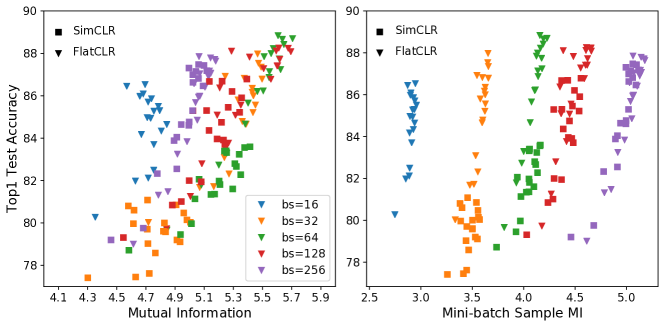
Figure S1: While ground-truth representation MI strongly correlates with performance (left), this relation is not evident with the mini-batch sample MI (right).

Figure S2: Speed up of large-batch training with ResNet-50 on Cifar. Larger batch leads to faster convergence.

E.3 Transfer learning and semi-supervised learning

Table S2: ImageNet SSL transfer learning results.

Dataset	Cifar10	Cifar100	VOC2007	Flower	SUN397
Linear evaluation
SimCLR	87.74	65.40	69.38	90.03	49.62
FlatCLR	87.92	65.76	69.66	90.23	51.31
Fine-tune
SimCLR	94.61	76.67	69.57	93.58	56.97
FlatCLR	95.50	78.92	70.73	95.02	58.37

Table S3: ImageNet SSL results.

Epoch	10	20	30	40	50	60	70	80	90	100
Top-1 Acc
SimCLR	40.93	46.22	48.64	50.14	52.14	53.62	55.20	56.36	56.99	57.13
FlatCLR	42.40	47.69	49.96	52.27	54.11	55.48	56.98	58.21	58.80	59.74
Top-5 Acc
SimCLR	65.34	70.92	73.63	75.38	76.90	78.24	79.59	80.58	80.85	81.00
FlatCLR	67.17	72.61	74.59	76.77	78.29	79.67	81.06	82.19	82.71	83.18

Table S4: ImageNet SSL semi-supervised learning results.

Label fraction	1%		10%
	Top1	Top5	Top1	Top5
Supervised	5.25	14.40	41.98	67.05
SimCLR	33.44	61.29	54.62	79.89
FlatCLR	36.35	64.59	56.51	81.32

Transfer Learning via a Linear Classifier

We trained a logistic regression classifier without $l_{2}$ regularization on features extracted from the frozen pretrained network. We used Adam to optimize the softmax cross-entropy objective and we did not apply data augmentation. As preprocessing, all images were resized to $224$ pixels along the shorter side using bicubic resampling, after which we took a $224\times 224$ center crop.

Transfer Learning via Fine-Tuning

We finetuned the entire network using the weights of the pretrained network as initialization. We trained for $100$ epochs at a batch size of $512$ using Adam with Nesterov momentum with a momentum parameter of $0.9$. At test time, we resized images to $256$ pixels along the shorter side and took a $224\times 224$ center crop. We fixed the learning rate = $5^{-5}$ and no weight decay in all datasets. As data augmentation during fine-tuning, we performed only random crops with resize and flips; in contrast to pretraining, we did not perform color augmentation or blurring.

Semi-supervised Learning Supervised Baselines

We compare against architecturally identical ResNet models trained on ImageNet with standard cross-entropy loss. These models are trained with the random crops with resize and flip augmentations and are also trained for 100 epochs.

E.4 Clarifications on the performance gaps to SOTA results

This paper aims for promote a novel contrastive learning objective FlatNCE that overcomes the limitations of the widely employed InfoNCE. While in all experiment we performed, our FlatNCE outperforms InfoNCE under the same settings, we acknowledge that there is still noticeable performance gap compared to SOTA results reported in literature. We want to emphasize this paper is more about bringing theoretical clarification to the problem, rather than beating SOTA solutions, which requires extensive engineering efforts and significant investment in computation, which we do not possess. For example, the SimCLR paper [1] have carried out extensive hyperparameter tuning for each model-dataset combination and select the best hyperparameters on a validation set. The computation resource assessible to us is dwarfed by such need. Their results on transfer learning and semi-supervised learning are transfered from a ResNet50 ($4\times$) (or ResNet50) with $4096$ batch size and $1000$ epochs training on SimCLR. Our results posted here are transfered from a ResNet50 with $512$ batch size and 100 epochs training on SimCLR and FlatCLR. Also, we chose to use the same hyperparameter and training strategy for each dataset to validate the generalization and present a fair comparison between SimCLR and FlatCLR.

All in all, the author(s) of this paper is absolutely confident that the proposed FlatCLR can help advance SOTA results. We invite the community to achieve this goal together.

References

- [1] T. Chen, S. Kornblith, M. Norouzi, and G. Hinton, “A simple framework for contrastive learning of visual representations,” in ICML, 2020.
- [2] N. Tishby and N. Zaslavsky, “Deep learning and the information bottleneck principle,” in 2015 IEEE Information Theory Workshop (ITW), pp. 1–5, IEEE, 2015.
- [3] R. D. Hjelm, A. Fedorov, S. Lavoie-Marchildon, K. Grewal, P. Bachman, A. Trischler, and Y. Bengio, “Learning deep representations by mutual information estimation and maximization,” in ICLR, 2019.
- [4] A. v. d. Oord, Y. Li, and O. Vinyals, “Representation learning with contrastive predictive coding,” arXiv preprint arXiv:1807.03748, 2018.
- [5] Z. Wu, Y. Xiong, S. X. Yu, and D. Lin, “Unsupervised feature learning via non-parametric instance discrimination,” in CVPR, 2018.
- [6] K. He, H. Fan, Y. Wu, S. Xie, and R. Girshick, “Momentum contrast for unsupervised visual representation learning,” in CVPR, 2020.
- [7] I. Misra and L. v. d. Maaten, “Self-supervised learning of pretext-invariant representations,” in CVPR, 2020.
- [8] T. Gao, X. Yao, and D. Chen, “Simcse: Simple contrastive learning of sentence embeddings,” arXiv preprint arXiv:2104.08821, 2021.
- [9] A. Radford, J. W. Kim, C. Hallacy, A. Ramesh, G. Goh, S. Agarwal, G. Sastry, A. Askell, P. Mishkin, J. Clark, et al., “Learning transferable visual models from natural language supervision,” arXiv preprint arXiv:2103.00020, 2021.
- [10] M. Laskin, A. Srinivas, and P. Abbeel, “Curl: Contrastive unsupervised representations for reinforcement learning,” in International Conference on Machine Learning, pp. 5639–5650, PMLR, 2020.
- [11] U. Gupta, A. Ferber, B. Dilkina, and G. V. Steeg, “Controllable guarantees for fair outcomes via contrastive information estimation,” arXiv preprint arXiv:2101.04108, 2021.
- [12] M. U. Gutmann and A. Hyvärinen, “Noise-contrastive estimation of unnormalized statistical models, with applications to natural image statistics,” Journal of Machine Learning Research, vol. 13, no. Feb, pp. 307–361, 2012.
- [13] B. Poole, S. Ozair, A. Van Den Oord, A. Alemi, and G. Tucker, “On variational bounds of mutual information,” in ICML, PMLR, 2019.
- [14] G. E. Hinton, “Training products of experts by minimizing contrastive divergence,” Neural Computation, vol. 14, no. 8, pp. 1771–1800, 2002.
- [15] T. Mikolov, I. Sutskever, K. Chen, G. Corrado, and J. Dean, “Distributed representations of words and phrases and their compositionality,” in NIPS, 2013.
- [16] A. Mnih and K. Kavukcuoglu, “Learning word embeddings efficiently with noise-contrastive estimation,” in NIPS, vol. 26, pp. 2265–2273, 2013.
- [17] Z. Ma and M. Collins, “Noise contrastive estimation and negative sampling for conditional models: Consistency and statistical efficiency,” arXiv preprint arXiv:1809.01812, 2018.
- [18] B. Perozzi, R. Al-Rfou, and S. Skiena, “Deepwalk: Online learning of social representations,” in SIGKDD, 2014.
- [19] A. Grover and J. Leskovec, “node2vec: Scalable feature learning for networks,” in SIGKDD, 2016.
- [20] P. H. Le-Khac, G. Healy, and A. F. Smeaton, “Contrastive representation learning: A framework and review,” IEEE Access, 2020.
- [21] S. Arora, H. Khandeparkar, M. Khodak, O. Plevrakis, and N. Saunshi, “A theoretical analysis of contrastive unsupervised representation learning,” ICML, 2019.
- [22] T. Wang and P. Isola, “Understanding contrastive representation learning through alignment and uniformity on the hypersphere,” in ICML, PMLR, 2020.
- [23] J. Robinson, C.-Y. Chuang, S. Sra, and S. Jegelka, “Contrastive learning with hard negative samples,” arXiv preprint arXiv:2010.04592, 2020.
- [24] Y. Kalantidis, M. B. Sariyildiz, N. Pion, P. Weinzaepfel, and D. Larlus, “Hard negative mixing for contrastive learning,” arXiv preprint arXiv:2010.01028, 2020.
- [25] C.-Y. Chuang, J. Robinson, L. Yen-Chen, A. Torralba, and S. Jegelka, “Debiased contrastive learning,” in NeurIPS, 2020.
- [26] L. Logeswaran and H. Lee, “An efficient framework for learning sentence representations,” arXiv preprint arXiv:1803.02893, 2018.
- [27] S. Ozair, C. Lynch, Y. Bengio, A. v. d. Oord, S. Levine, and P. Sermanet, “Wasserstein dependency measure for representation learning,” NeurIPS, 2019.
- [28] O. Henaff, “Data-efficient image recognition with contrastive predictive coding,” in ICML, PMLR, 2020.
- [29] M. Wu, C. Zhuang, D. Yamins, and N. Goodman, “On the importance of views in unsupervised representation learning,” preprint, vol. 3, 2020.
- [30] K. Nozawa and I. Sato, “Understanding negative samples in instance discriminative self-supervised representation learning,” arXiv preprint arXiv:2102.06866, 2021.
- [31] M. Tschannen, J. Djolonga, P. K. Rubenstein, S. Gelly, and M. Lucic, “On mutual information maximization for representation learning,” ICLR, 2020.
- [32] J. Song and S. Ermon, “Understanding the limitations of variational mutual information estimators,” in ICLR, 2020.
- [33] D. McAllester and K. Stratos, “Formal limitations on the measurement of mutual information,” arXiv preprint arXiv:1811.04251, 2018.
- [34] P. Bachman, R. D. Hjelm, and W. Buchwalter, “Learning representations by maximizing mutual information across views,” in NeurIPS, 2019.
- [35] C. Jia, Y. Yang, Y. Xia, Y.-T. Chen, Z. Parekh, H. Pham, Q. V. Le, Y. Sung, Z. Li, and T. Duerig, “Scaling up visual and vision-language representation learning with noisy text supervision,” arXiv preprint arXiv:2102.05918, 2021.
- [36] C. E. Shannon, “A mathematical theory of communication,” The Bell system technical journal, vol. 27, no. 3, pp. 379–423, 1948.
- [37] D. J. MacKay, Information theory, inference and learning algorithms. Cambridge university press, 2003.
- [38] D. N. Reshef, Y. A. Reshef, H. K. Finucane, S. R. Grossman, G. McVean, P. J. Turnbaugh, E. S. Lander, M. Mitzenmacher, and P. C. Sabeti, “Detecting novel associations in large data sets,” Science, vol. 334, no. 6062, pp. 1518–1524, 2011.
- [39] A. Gretton, R. Herbrich, and A. J. Smola, “The kernel mutual information,” in ICASSP, IEEE, 2003.
- [40] A. Kraskov, H. Stögbauer, and P. Grassberger, “Estimating mutual information,” Physical review E, vol. 69, no. 6, p. 066138, 2004.
- [41] F. Pérez-Cruz, “Estimation of information theoretic measures for continuous random variables,” in NIPS, 2008.
- [42] S. Gao, G. Ver Steeg, and A. Galstyan, “Efficient estimation of mutual information for strongly dependent variables,” in AISTATS, PMLR, 2015.
- [43] T. Suzuki, M. Sugiyama, J. Sese, and T. Kanamori, “Approximating mutual information by maximum likelihood density ratio estimation,” in New challenges for feature selection in data mining and knowledge discovery, pp. 5–20, PMLR, 2008.
- [44] M. I. Belghazi, A. Baratin, S. Rajeshwar, S. Ozair, Y. Bengio, A. Courville, and D. Hjelm, “Mutual information neural estimation,” in ICML, PMLR, 2018.
- [45] D. Moyer, S. Gao, R. Brekelmans, G. V. Steeg, and A. Galstyan, “Invariant representations without adversarial training,” in NeurIPS, 2018.
- [46] P. Cheng, W. Hao, S. Dai, J. Liu, Z. Gan, and L. Carin, “CLUB: A contrastive log-ratio upper bound of mutual information,” in ICML, 2020.
- [47] M. Gutmann and A. Hyvärinen, “Noise-contrastive estimation: A new estimation principle for unnormalized statistical models,” in AISTATS, pp. 297–304, 2010.
- [48] Y. Tian, D. Krishnan, and P. Isola, “Contrastive multiview coding,” arXiv preprint arXiv:1906.05849, 2019.
- [49] P. Bojanowski and A. Joulin, “Unsupervised learning by predicting noise,” in ICML, PMLR, 2017.
- [50] W. Fenchel, “On conjugate convex functions,” Canadian Journal of Mathematics, vol. 1, no. 1, pp. 73–77, 1949.
- [51] C. Tao, L. Chen, S. Dai, J. Chen, K. Bai, D. Wang, J. Feng, W. Lu, G. Bobashev, and L. Carin, “On Fenchel mini-max learning,” in NeurIPS, 2019.
- [52] Q. Guo, J. Chen, D. Wang, Y. Yang, X. Deng, F. Li, L. Carin, and C. Tao, “Tight mutual information estimation with contrastive Fenchel-Legendre optimization,” 2021. [Available online; accessed 28-May-2021].
- [53] H. Robbins and S. Monro, “A stochastic approximation method,” The annals of mathematical statistics, pp. 400–407, 1951.
- [54] L. Bottou, “Large-scale machine learning with stochastic gradient descent,” in Proceedings of COMPSTAT’2010, pp. 177–186, Springer, 2010.
- [55] N. S. Keskar, D. Mudigere, J. Nocedal, M. Smelyanskiy, and P. T. P. Tang, “On large-batch training for deep learning: Generalization gap and sharp minima,” arXiv preprint arXiv:1609.04836, 2016.
- [56] P. Goyal, P. Dollár, R. Girshick, P. Noordhuis, L. Wesolowski, A. Kyrola, A. Tulloch, Y. Jia, and K. He, “Accurate, large minibatch sgd: Training imagenet in 1 hour,” arXiv preprint arXiv:1706.02677, 2017.
- [57] Y. Burda, R. Grosse, and R. Salakhutdinov, “Importance weighted autoencoders,” in ICLR, 2016.
- [58] T. Rainforth, T. A. Le, M. I. C. J. Maddison, and Y. W. T. F. Wood, “Tighter variational bounds are not necessarily better,” in NIPS workshop, 2017.
- [59] A. Hyvarinen, H. Sasaki, and R. Turner, “Nonlinear ica using auxiliary variables and generalized contrastive learning,” in AISTATS, pp. 859–868, 2019.
- [60] M. D. Donsker and S. S. Varadhan, “Asymptotic evaluation of certain markov process expectations for large time. iv,” Communications on Pure and Applied Mathematics, vol. 36, no. 2, pp. 183–212, 1983.
- [61] X. Nguyen, M. J. Wainwright, and M. I. Jordan, “Estimating divergence functionals and the likelihood ratio by convex risk minimization,” IEEE Transactions on Information Theory, vol. 56, no. 11, pp. 5847–5861, 2010.
- [62] J.-B. Hiriart-Urruty and C. Lemaréchal, Fundamentals of convex analysis. Springer Science & Business Media, 2012.
- [63] D. Barber and F. Agakov, “The IM algorithm: a variational approach to information maximization,” Advances in neural information processing systems, vol. 16, p. 201, 2004.