Interplay between singlet and triplet pairings in multi-band two-dimensional oxide superconductors

Abstract

We theoretically study the superconducting properties of multi-band two-dimensional transition metal oxide superconductors by analyzing not only the role played by conventional singlet pairings, but also by the triplet order parameters, favored by the spin-orbit couplings present in these materials. In particular, we focus on the two-dimensional electron gas at the (001) interface between $LaAlO_{3}$ and $SrTiO_{3}$ band insulators where the low electron densities and the sizeable spin-orbit couplings affect the superconducting features. Our theoretical study is based on an extended superconducting mean-field analysis of the typical multi-band tight-binding Hamiltonian, as well as on a parallel analysis of the effective electronic bands in the low-momentum limit, including static on-site and inter-site intra-band attractive potentials under applied magnetic fields. The presence of triplet pairings is able to strongly reduce the singlet order parameters which, as a result, are no longer a monotonic function of the charge density. The interplay between the singlet and the triplet pairings affects the dispersion of quasi-particle excitations in the Brillouin zone and also induces anisotropy in the superconducting behavior under the action of an in-plane and of an out-of-plane magnetic fields. Finally, non-trivial topological superconducting states become stable as a function of the charge density, as well as of the magnitude and of the orientation of the magnetic field. In addition to the chiral, time-reversal breaking, topological superconducting phase, favored by the linear Rashba couplings and by the on-site attractive potentials in the presence of an out-of-plane magnetic field, we find that a time-reversal invariant topological helical superconducting phase is promoted by not-linear spin-orbit couplings and by the inter-site attractive interactions in the absence of magnetic field.

I Introduction

The transition metal oxides represent a large class of materials with functional properties not only in the bulk but also in hetero-structures and nano-structures. In particular, the two-dimensional electron gas (2DEG) at the (001) interface between $LaAlO_{3}$ (LAO) and $SrTiO_{3}$ (STO) band insulators has gained a continuously growing interest in recent years, as an ideal playground to investigate the interplay between magnetism, superconductivity, and spin-orbit coupling. Indeed, the 2DEG hosts a complex phase diagram, depending on the electron density Caviglia2 ; biscaras2 , on the temperature and on the applied magnetic field.

It is well known that LAO/STO 2DEGs host an unconventional superconducting regime, achievable by tuning the applied gate voltage. The origin of the superconductivity is still not understood Gorkov2016 ; Edge2015 ; Ruhman2016 ; gariglio2016 ; tafuri2017 , and various open questions remain unsolved about the role of quantum electronic correlations maniv2015strong ; Monteiro2019 , of multiband effects Trevisan2018 ; Wojcik2020 ; zeg2020 ; jouan2021 , and of the spin-orbit coupling Khalsa2013 ; Diez2015 ; Zhong2013 ; Shalom2010 ; Rout2017 . Moreover, the possibility of topological superconductivity is also under debate Scheurer ; Mohanta ; Loder ; Fukaya ; settino2020 ; santamaria2021 ; tafuri2017 ; perroni2019 .

Even more interestingly, the superconducting critical temperature, $T_{c}$, in the LAO/STO 2DEG exhibits a dome-shape behavior, as a function of the applied gate voltage Reyren ; Rout2017 ; joshua2012universal ; maniv2015strong ; biscaras2 ; biscaras2010two ; Caviglia2 . When the carrier density increases, $T_{c}$ first increases up to a maximum value, $T_{c}^{\mathrm{max}}$ $\simeq$ 300 mK, at an optimal effettive doping, then it starts to decrease. The resulting phase diagram is qualitatively very similar to that of high $T_{c}$ cuprates, of organic superconductors, of Fe-based superconductors, as well as of heavy fermions taillefer ; keimer . Recently, the shape of the superconducting dome has been qualitatively explained by assuming a particular real-space potential, effectively attractive in suitable windows of momentum space, and resulting into an extended s-wave pairing zeg2020 . Moreover, a forthcoming insightful work paramekanti2020 showed that the formation of a similar dome (or even many of them, when multiband fermionic models are considered) is related generically to an attractive potential with finite range. The same work shed light on previous works, where the dome has been suggested instead as an effect of the spin-orbit coupling Shalom2010 ; Rout2017 ; Yin2019 ; singh2018gap . Furthermore, an asymmetric response in shear-resistivity to an applied magnetic field (in-plane or out-of-plane) has been observed caviglia2009 : a similar asymmetry can suggest a possible spatial asymmetry in the pairing.

To address the open questions above, in this paper we discuss the superconductivity in LAO/STO 2DEG, by making a singlet-triplet mixed ansatz for the pairing and by studying its physical consequences. This possibility looks pretty natural, due to the inversion symmetry breaking term of the heterostructure which gives rise to an effective Rashba-like coupling, already known to favour mixed pairings rashba2001 ; tafuri2017 ; alidoust2021 . Related notable effects are qualitative deviations of the standard BCS/BEC crossover pieri2019 . The same possibility has been corroborated quite recently, using a Monte-Carlo approach on a square lattice rosenberg2017 : there, even a local (Hubbard) interaction proved sufficient for singlet-triplet mixing, provided that a Rashba coupling is added. Interestingly, a singlet-triplet mixed pairing allows (but does not imply) edge excitations, protected by a nontrivial topology, whose presence has not been ruled out so far by current transport experiments. Moreover, it determines an asymmetric response to an applied magnetic field, qualitatively similar to that observed in caviglia2009 . We finally notice that, while a pure triplet p-wave pairing is ruled out by previous experiments which did not detect the expected nodes in the superconducting gap hwang2018 ; sumita2020 , instead a singlet-triplet mixed pairing would not contradict the experimental results.

In this paper, we employ a tight-binding model including the low-energy electronic structure of the LAO/STO 2DEG with the ${d_{xy},d_{xz},d_{yz}}$ orbitals of the Ti atoms popovic ; delugas ; scopigno ; salluzzo ; Khalsa2013 . Various papers have pointed out the close relation between the onset of the superconductivity and the filling of the degenerate $d_{xz/yz}$ sub-bands, at an high density of states valentinis ; singh . Then, we adopt an attractive static potential, with both local and nearest-neighbour terms, able to host all the pairing configurations mentioned above. In addition, we include the atomic spin-orbit and the inversion asymmetric potential associated with the orbital Rashba interaction. Finally, we consider a magnetic field as a source of time reversal symmetry breaking. To achieve our results, we perform a detailed analysis of the most favorable topological superconducting phases. This analysis is based on self-consistent computations of the order parameters, minimizing the mean-field free energy in the Hamiltonian parameters space, set by the electron filling, by the attraction strengths, and by the amplitude and orientation of the magnetic field.

We point out how the interplay of singlet and triplet pairings is able to affect the superconducting properties of LAO/STO 2DEGs. First, we show that the singlet order parameters are strongly reduced with increasing the role of triplet pairings, thus acquiring a non-monotonic dependence on the charge density. Interestingly, some notable effects are found related with not-linear corrections to the effective Rashba spin-orbit coupling. For instance, in the absence of magnetic fields, the not-linear spin-orbit terms, combined with the triplet pairings, favor a quite stable (time-reversal invariant) topological helical superconducting phase. The triplet pairings are also responsible for an anisotropic behavior of the superconducting order parameters, when the magnetic field is applied in-plane and out-of-plane. Finally, in the presence of out-of-plane magnetic fields, we recover (time-reversal breaking) chiral topological superconducting phases, also when the triplet pairings are vanishing.

The paper is organized as follows:

In Section II, we report the main electronic properties of the normal state.

In Section III, we discuss the general set-up of the mean-analysis of superconductivity.

In Section IV, we analyze the superconducting solutions at zero magnetic field.

In Section V, we analyze the effects of a magnetic field.

Finally, we devote Section VI to our conclusions and outlook.

II Normal state

II.1 Model Hamiltonian

Following the derivation of Ref. [perroni2019, ], we write down the general tight-binding Hamiltonian for the two-dimensional LAO/STO-001 system by considering the 2DEG effectively confined on a square with lattice step $a=3.9\,\AA\equiv 1$. The system has also a broken out-of-plane inversion symmetry, having only the $t_{2g}$-orbitals close to the Fermi level. In LAO/STO systems, the transition metal (TM)-oxygen bond angle is almost ideal, and the three $t_{2g}$-bands are mainly decoupled in the momentum space ${\bf k}$.

Figure 1: Plot of $\epsilon_{yz}{\color[rgb]{0,0,0}({\bf k})}$, $\epsilon_{zx}{\color[rgb]{0,0,0}({\bf k})}$, and $\epsilon_{xy}{\color[rgb]{0,0,0}({\bf k})}$ (left panel, in meV), and of the mixed bands $\epsilon_{-,0,+}{\color[rgb]{0,0,0}({\bf k})}$ (middle and right panels), in the absence of magnetic field, for $k_{y}=0$, and as functions of $k_{x}$ (still around $k_{x}=0$, then for $\nu\to 0$). In the middle panel, around $k_{x}\approx 0.35$, we have avoided crossings, due to the role of the atomic spin-orbit coupling and the breaking inversion symmetry term.

Moreover, the $d_{xy}$ band has a truly two-dimensional character, while the $d_{yz}$ and $d_{zx}$ bands are quasi one-dimensional. In the following, we denote with $H_{0}({\bf k})$ the corresponding normal-state contribution to the total system Hamiltonian in momentum space. Moreover, herewith we use the index $\tau=\{yz,zx,xy\}$ to refer to the three different $t_{2g}$ orbitals $d_{yz}$, $d_{zx}$, and $d_{xy}$, respectively, while we label the spin with $\sigma=\{\uparrow,\downarrow\}$. In addition, we add a term $H_{SO}$ to the total Hamiltonian, accounting for the atomic spin-orbit coupling of the TM ions. Finally, we include the microscopic couplings arising from the out-of-plane oxygen displacements around the TM, with the inversion asymmetry giving rise to an effective hybridization of $d_{xy}$ and $d_{yz}$ or $d_{zx}$-orbitals along the $y$ or $x$ directions, respectively. We denote this contribution as $H_{Z}({\bf k})$.

In momentum space, we set

$${\cal H}=\hat{D}^{\dagger}({\bf k})H({\bf k})\hat{D}({\bf k})\>\>,$$ (1)

with $\hat{D}({\bf k})$ labelling the vector

$$[c_{yz,\uparrow}({\bf k}),c_{yz,\downarrow}({\bf k}),c_{zx,\uparrow}({\bf k}),c_{zx,\downarrow}({\bf k}),c_{xy,\uparrow}({\bf k}),c_{xy,\downarrow}({\bf k})]_{t}\>,$$ (2)

(note the different grouping of the operators corresponding to the various orbitals with respect to perroni2019 ), and

$$H({\bf k})=\sum_{\tau}H_{\tau}({\bf k})=H_{0}({\bf k})+H_{\rm SO}+H_{Z}({\bf k})+H_{M}\>\>\>\>.$$ (3)

The various terms at the right-hand side of Eq. (3) are grouped as follows. The first term $H_{0}({\bf k})$ is the lattice band term

$$H_{0}({\bf k})=\left[\begin{array}[]{ccc}\epsilon_{yz}{\color[rgb]{0,0,0}({\bf k})}{\bf I}_{2\mathrm{x}2}&{\bf 0}&{\bf 0}\\ {\bf 0}&\epsilon_{zx}{\color[rgb]{0,0,0}({\bf k})}{\bf I}_{2\mathrm{x}2}&{\bf 0}\\ {\bf 0}&{\bf 0}&\epsilon_{xy}{\color[rgb]{0,0,0}({\bf k})}{\bf I}_{2\mathrm{x}2}\end{array}\right]\;,$$ (4)

with

$$\epsilon_{yz}{\color[rgb]{0,0,0}({\bf k})} = 2t_{1y}[1-\cos(k_{y})]+2t_{2x}[1-\cos(k_{x})]$$

$$\epsilon_{zx}{\color[rgb]{0,0,0}({\bf k})} = 2t_{1x}[1-\cos(k_{x})]+2t_{2y}[1-\cos(k_{y})]$$

$$\epsilon_{xy}{\color[rgb]{0,0,0}({\bf k})} = 4t_{1}-2t_{1x}\cos(k_{x})-2t_{1y}\cos(k_{y})+E_{t}\,,$$ (5)

and the parameters set so that

$$t_{1x}=t_{1y}\equiv t_{1}=300\>{\rm meV}$$

$$t_{2x}=t_{2y}\equiv t_{2}=20\>{\rm meV}$$

$$E_{t}=-50\>{\rm meV}\,.$$ (6)

The second term in Eq.(3) is the atomic $l-s$ spin-orbit coupling term, given by

$$H_{\rm SO}=w_{{\rm SO}}\,\hat{{\bf l}}\otimes{\bf\sigma},$$ (7)

with $\hat{{\bf l}}$ the vector operator describing the orbital angular momentum and ${\bf\sigma}$ (the Pauli matrices) the spin angular momentum. In order to make the spin-orbit term explicit, we introduce the matrices $\hat{l}_{x}$, $\hat{l}_{y}$ and $\hat{l}_{z}$, which are the projections of the $l=2$ angular momentum operator onto the $t_{2g}$ subspace,

$$\hat{l}_{x} =\begin{pmatrix}0&0&0\\ 0&0&i\\ 0&-i&0\end{pmatrix},$$ (8)

$$\hat{l}_{y} =\begin{pmatrix}0&0&-i\\ 0&0&0\\ i&0&0\end{pmatrix},$$ (9)

$$\hat{l}_{z} =\begin{pmatrix}0&i&0\\ -i&0&0\\ 0&0&0\end{pmatrix},$$ (10)

assuming $\{yz,zx,xy\}$ as orbital basis. Using these operators, we write the atomic spin-orbit coupling as

$${\color[rgb]{0,0,0}H_{\rm SO}=i{\color[rgb]{0,0,0}w_{{\rm SO}}}\left[\begin{array}[]{ccc}{\bf 0}&{\bf\sigma}_{z}&-{\bf\sigma}_{y}\\ -{\bf\sigma}_{z}&{\bf 0}&{\bf\sigma}_{x}\\ {\bf\sigma}_{y}&-{\bf\sigma}_{x}&{\bf 0}\end{array}\right]}\>\>\>\>,$$ (11)

with ${\color[rgb]{0,0,0}w_{\rm SO}}=10\>{\rm meV}$.

The third term in Eq. (3) is the inversion symmetry breaking term $H_{Z}({\bf k})$, given by

$$H_{Z}({\bf k})=\gamma\left[\hat{l}_{y}\otimes{\bf I}_{2\mathrm{x}2}\sin{k_{x}}-\hat{l}_{x}\otimes{\bf I}_{2\mathrm{x}2}\sin{k_{y}}\right],$$ (12)

or equivalently

$$H_{Z}({\bf k})=i\gamma\left[\begin{array}[]{ccc}{\bf 0}&{\bf 0}&-\sin(k_{x}){\bf I}_{2\mathrm{x}2}\\ {\bf 0}&{\bf 0}&-\sin(k_{y}){\bf I}_{2\mathrm{x}2}\\ \sin(k_{x}){\bf I}_{2\mathrm{x}2}&\sin(k_{y}){\bf I}_{2\mathrm{x}2}&{\bf 0}\end{array}\right]\;\;\;\;,$$ (13)

with $\gamma=20\>{\rm meV}$. This important term stems from the breakdown of a reflection symmetry along a particular axis of the LAO/STO compounds, due to a corresponding lattice distortion. The net effect is the mixing of the different orbitals $yz$, $zx$, and $xy$, having different parity under the mentioned reflection symmetry. More details are in perroni2019 . Furthermore, the effects of the coupling $\gamma$ on the stability of singlet and triplet superconducting order parameters will be discussed in Appendix 5.

The last term in Eq. (3) describes the coupling of the electron spin and orbital moments with an external magnetic field B, whose direction is given by the vector ${\bf M}=-\mu_{B}{\bf B}/\hbar$, with $\mu_{B}$ Bohr magneton:

$$H_{M}=g_{s}\,{\bf I}_{3\mathrm{x}3}\otimes{\bf M}\cdot\frac{{\bf\sigma}}{2}+{\bf M}\cdot{\bf\l}\otimes{\bf I}_{2\mathrm{x}2}\,,$$ (14)

which includes the gyromagnetic factor $g_{s}$ assumed equal to 2. In the absence of this term, the total Hamiltonian is time-reversal invariant:

$$H({\bf k})=U_{T}^{-1}H^{*}(-{\bf k})U_{T}\,,\quad\quad\quad U_{T}={\bf I}_{3\mathrm{x}3}\otimes\sigma_{y}$$ (15)

($\sigma_{y}$ acting on the spin index $\sigma$, ${\bf I}_{3\mathrm{x}3}$ on the $\tau$ index, and $U_{T}\,U_{T}^{*}=-{\bf I}_{3\mathrm{x}3}$), as it can be straightforwardly checked by expressing $H({\bf k})$ in terms e. g. of Gell-Mann matrices (see Appendix 1). Therefore, in the absence of superconductive pairing, $H({\bf k})$ belongs to the class AII of the classification for topological insulators and superconductors, see e.g. ludwig2009 ; ryu2016 ; Bernevigbook .

In the following part of the Section, we will analyze the bands in the normal state in the absence of the external magnetic field. The external field weakly affects the electronic structure of the normal state, but its role will be relevant in the analysis of the superconducting phases since the low energy induced by the field competes with those due to the superconducting pairings.

II.2 Band structure

In the left panel of Fig. 1 we show the ”bare” $\tau$ bands, which we derived by setting to zero both the spin-orbit coupling and the inversion symmetry breaking term. We notice that the lowest band is the $xy$ one, separated by the energy $|E_{t}|$ from the $yz$ and $zx$ bands, which are degenerate at $k_{x}=0$. In the same figure, we plot the bands, as a function of $k_{x}$, at $k_{y}=0$. We identify the almost flat band with the $yz$ one and we also note that the dispersion of the $zx$ band is negligible as a function of $k_{y}$ and at fixed $k_{x}$.

Introducing the spin-orbit coupling and the inversion symmetry breaking term, the $\tau$-bands are mixed together by the rotation matrix $M(\bf{k})$ that diagonalizes $H(\bf{k})$. Therefore, the orbital character is mixed, giving rise to a more complex spectrum perroni2019 and to new, “mixed” bands, which in the following we label with the indices $\eta_{\{-,0,+\}}$. In fact, we see that the spin-orbit coupling and the inversion symmetry breaking mostly affect the electronic bands at low densities. To evidence this fact, in the central and right panels of Fig. 1, we report these bands, which at finite values of the momentum exhibit avoided crossing. In particular, in the right panel of Fig. 1, we focus on small values of the momenta. We see that the $\eta_{\pm}$-bands display minima at finite momenta, which is traced back to an emerging effective linear Rashba coupling (see Ref. [perroni2019, ] and the next subsection). On the other hand, $\eta_{0}$ shows a single minimum at ${\bf k}=0$, indicating an enhanced importance of not-linear corrections.

In the following, we will carefully investigate the behavior of the $\eta_{0}$-band at small values of ${\bf k}$. In fact, the minima of the $\eta_{0}$-band mark the density values where superconductivity sets in. Indeed, theoretical and experimental studies suggest the presence of superconducting phases in the range for the lattice average filling $\nu$ approximately between the onset of the $\eta_{0}$ band and that of the $\eta_{+}$ band (see e.g. gariglio2016 ).

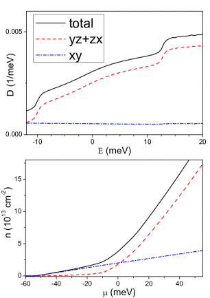
Figure 2: Upper panel: density of states of the $\tau$-bands, as a function of the single-particle energy. Lower panel: carrier surface density, as a function of the chemical potential.

Therefore, we focus on the electronic properties within this density range. In the upper panel of Fig. 2, we plot the density of states (DOS) of the $\eta$-bands, as a function of the single-particle energy (note that the density has the dimensions of the inverse of an energy, since we set the lattice step $a=1$). The minima of the bands are characterized by steps in the density of states. In the same panel, the projection of the DOS on the orbital basis $xy$, $yz$, and $zx$ is also reported, such to highlight their contributions. We remark that the quasi-one-dimensional bands $yz$ and $zx$ provide the most relevant contribution to the density of states. Actually, within this energy range, the density of states due to the $xy$ band is almost constant, after a step at much lower energy (of the order of $E_{t}$). This asymmetry in the density of states within this energy range will be fundamental for the interpretation of some superconducting properties, which are very sensitive to the magnitude of the available electronic states. Finally, within a slightly larger energy range, in the lower panel of Fig. 2, we plot the carrier space density, as a function of the chemical potential. For the parameters of the tight-binding model used in this paper, the density at the minimum of $yz$ and $zx$ bands is about $2\cdot 10^{13}$ $cm^{-2}$. This value is in agreement with previous experimental results Stornaiuolo . Moreover, we notice that, in analogy with the behavior of the density of states, as soon as the quasi-one-dimensional $yz$ and $zx$ bands start to be filled, they rapidly become predominant. This occurs around zero energy, where a crossover in the densities is visible. There, the carrier density, of the order of $5\cdot 10^{13}$ $cm^{-2}$, results half from the $xy$ band and half from the $yz$ and $zx$ ones.

II.3 Effective low-energy theories

In order to better spell out the following results, we now present an effective theory for the $\eta_{-}$- and $\eta_{0}$-bands, around their common minima, at $k_{x}=k_{y}=0$. To derive the corresponding Hamiltonians we exploit the second order degenerate perturbation theory. We present the details of our derivation in Appendix 3. The results are respectively:

$$H_{-}^{(\mathrm{eff})}({\bf k})=\epsilon_{-}({\bf k})\,{\bf I}-(a_{1}\,k_{x}+a_{2}\,k_{x}^{3})\,\sigma_{y}+(a_{1}\,k_{y}+a_{2}\,k_{y}^{3})\,\sigma_{x}\,,$$ (16)

with $a_{1}=8$ meV (in units of the lattice step $a\equiv 1$), $a_{2}=43.46$ meV, $\epsilon_{-}({\bf k})=\big{(}-54.+280.8\,(k_{x}^{2}+k_{y}^{2})\big{)}$ meV (so that $t_{-}^{(\mathrm{eff})}=280.8$ meV), and

$$H_{0}^{(\mathrm{eff})}({\bf k})=\left[\begin{array}[]{c}\epsilon_{0}({\bf k})\quad\quad i\,a_{3}\,k_{-}-i\,a_{4}\,k_{+}^{3}-a_{5}\,k_{x}k_{y}\,k_{+}\\ {}\hfil\\ -i\,a_{3}\,k_{+}+i\,a_{4}\,k_{-}^{3}-a_{5}\,k_{x}k_{y}\,k_{-}\quad\quad\epsilon_{0}({\bf k})\\ \end{array}\right]\,,$$ (17)

with $k_{\pm}=k_{x}\pm ik_{y}$, $a_{3}=0.8$ meV, $a_{4}=8.627$ meV, $a_{5}=22.8$ meV and $\epsilon_{0}({\bf k})=\big{(}-10.8+157.2\,(k_{x}^{2}+k_{y}^{2})\big{)}$ meV (so that $t_{0}^{(\mathrm{eff})}=157.2$ meV).

We notice that, around the minima of the $\eta$ bands, $k_{x}=k_{y}=0$, an effective linear Rashba-like spin-orbit coupling appears in both the effective Hamiltonians, together with a not-linear spin-orbit term. This second term is especially relevant for the first dome on the $\eta_{0}$ band, already at vanishing filling, as the central and right panels of Fig. 1 suggest. It is known rashba2001 that the linear coupling, breaking space inversion symmetry (as $H_{Z}({\bf k})$ it derives from), favours triplet components for superconducting pairings, inducing single-triplet mixings, see e. g. annett ; brydon2015 . Instead, not-linear spin-orbit terms have been postulated to induce observable modifications on the spin polarization in inversion symmetric (001) $SrTiO_{3}$ compounds nakamura2012 and for Josephson junctions alidoust2021 . Other notable effects will be described in the following.

In Fig. 11 of Appendix 3, we perform a direct comparison of $H_{-}^{(\mathrm{eff})({\bf k})}$ and $H_{0}^{(\mathrm{eff})}({\bf k})$ with the exact spectrum of $H({\bf k})$ in Eq. (1). We see that the agreement is excellent up to $k_{x,y}\approx 0.2$. This value must be compared with the typical momenta where the $\eta_{+}$ band starts to be populated, around $k_{x,y}=0.4$. The corresponding filling is estimated to be approximately the end of the superconductive dome gariglio2016 . Therefore, we expect $H_{0}^{(\mathrm{eff})}({\bf k})$ to describe approximately a low-density half of the first dome. Importantly, $H_{-}^{(\mathrm{eff})}({\bf k})$ and $H_{0}^{(\mathrm{eff})}({\bf k})$, that are a central result in the present work, still act on the $\sigma=\{\uparrow,\downarrow\}$ indices, that are not mixed each others along the perturbation theory procedure.

III Mean-field analysis of superconductivity: general set-up

In this Section we analyze the possible presence of superconducting phases, within the same energy and density ranges, and focusing in particular on the interplay of singlet and triplet pairings.

III.1 Setting up the effective interaction Hamiltonian

In order to induce superconductivity in the 2DEG, in the following we consider a pertinent, nearly realistic, attractive electronic interaction, together with its effects on the bands of $H({\bf k})$. In particular, in the absence of more specific coupling mechanism related to, e.g., antiferromagnetic correlations, we rely on the “natural” mechanism, based on phonon exchange plus screened Coulomb repulsion. While the phonon attraction is expected to be independent of the orbital index $\tau$, the Coulomb repulsion is expected to be more important within the same orbital, due to the larger overlaps between the electronic wavefunctions. Therefore, in the low density regime analyzed in this paper, we choose the realistic attractive potential given by:

$$W=-\sum_{i,j,\tau,\sigma,\sigma^{\prime}}U_{i,j}\,n_{i\tau\sigma}\,n_{j\tau\sigma^{\prime}}-\sum_{i,j,\tau,\tau^{\prime}\neq\tau,\sigma,\sigma^{\prime}}Z_{i,j}\,n_{i\tau\sigma}\,n_{j\tau^{\prime}\sigma^{\prime}}\,,$$ (18)

with the decay of $U_{i,j}$ and $Z_{i,j}$, with the separation $i-j$, ruled by two different lengths $\xi_{U}$ and $\xi_{V}$. The same lengths depend on the electronic density $\rho_{e}$, that is, on the lattice average filling $\nu$, and are expected to be of the order of a few lattice steps. Moreover, we assume a static potential, consistently with the low charge density in the regime of Fermi energies that we are considering. Actually, the dynamic part of the potential from the phonon exchange can be extrapolated to the low-energy limit, therefore the effective attractive potential at the Fermi energy can be assumes as static mazin2011 ; cataudella2021 .

The bands $\tau$, $\tau^{\prime}$ are mixed together by the rotation matrix $M(\bf{k})$ that diagonalizes $H(\bf{k})$; $M(\bf{k})$ accordingly affects the potential $W$ in Eq. (18), as well. It is difficult to deal with the transformed potential, since $M(\bf{k})$ depends on $\bf{k}$ and the Fourier transform of $W$ contains 4 momenta $\bf{k}_{i}$, $i=1,\dots,4$.

Therefore, in this paper we analyze the effects, especially on the topology, of the full potential $W$, focusing on its first term, diagonal on the orbital index $\tau$. This choice is motivated by the energy gap between the $\eta_{-}$ and $\eta_{0}$ bands around ${\bf k}=0$, where the superconductive dome is located gariglio2016 , being approximately $\delta E_{\eta}=43$ meV. This gap is an obstruction for the zero-momentum pairings between (unbalanced species in) the bands, and forbids them from attractions such that the superconductive gap, calculated at vanishing unbalance, is under a threshold around $\delta E_{\eta}$ (see pethick ; marchetti2007 ; rad2007 and references therein). Furthermore, nonzero-momentum balanced pairings are known to require at least a subtle fine-tuning between interaction and density pethick ; marchetti2007 ; rad2007 ; pieri2019 .

Within the tight-binding model, we focus on the on-site and the nearest neighbor contribution of the attractive potential between electrons in states with the same orbital symmetry. The local interaction necessarily couples electrons with opposite spins favoring spin-singlet symmetry. On the other hand, we assume that the term due to the nearest neighbors takes into account the equal spin contribution controlling the spin-triplet instability. Hence, we simplify $W$ according to

$$W=-U\sum_{i,\tau}n_{i\tau\uparrow}\,n_{i\tau\downarrow}-\frac{V}{2}\sum_{i\delta\tau\sigma}n_{i\tau\sigma}\,n_{i+\delta\tau\sigma}$$ (19)

where $i$ and $j$ label two dimensional vectors associated to the lattice sites, $U$ and $V$ are the local and nearest neighbor pairing energy, respectively, and $n_{i\tau\sigma}=c_{i\tau\sigma}^{\dagger}c_{i\tau\sigma}$ is the local density operator for the $\sigma$ spin polarization and the $\tau$ orbital, at a given position $i$, whose nearest neighbor sites are indicated by $\delta$. In Appendix 4, we discuss additional attractive terms which have not been introduced in Eq. (19).

As specified in the subsection title, we have considered in Eq. (19) an effective interaction, in particular an attractive local Hubbard term. We note that in breit2010 a local repulsive Hubbard term, around 2 eV, has been predicted from tunneling spectroscopy. In fact, this value of U is not large, but it is comparable with the electron bandwidth. Furthermore, in LAO/STO systems analyzed in this paper, the typical densities per spin polarization are low compared to, e.g. , the half-filling regime. Accordingly, the net contribution to the total energy from Hubbard interaction is limited. Moreover, it is known that, in these density regimes, the effects from polaron dynamics are relevant on the electronic states cancellieri2016 ; cataudella2021 giving rise to a net lowering of the Hubbard interaction for the 2D quantum gas. Finally, our effective model for the local interaction has been widely used in the literature, for example Mohanta ; Loder ; Fukaya ; perroni2019 ; settino2020 quoted in the introduction.

In the following, we will check that $W$ in Eq. (19) qualitatively reproduces the most interesting features of superconductivity in LAO/STO compounds gariglio2016 , with the values of $U$ and $V$, yielding the superconducting behavior discussed in this paper always, being of the order of hundreds of meV.

III.2 Mean field analysis

We now analyze, within mean-field approximation, the Hamiltonian in Eq. (1), with the interaction in Eq. (19), by mostly focusing onto the zero temperature case.

Due to the introduction of the nearest neighbor attractive term $V$, it becomes important to properly infer the profile of the superconducting order parameter in real space. In the following, we do so by encompassing within our mean-field approach both the spin and the orbital degrees of freedom. In particular, we recover the appropriate pairing ansatz by analyzing the set of the irreducible representations of the point-group symmetry of the square lattice, by assuming over-all translational invariance (we provide the details in Appendix 2). Moreover, in the absence of an externally-applied magnetic coupling, we retain time-reversal invariance. As a result, we obtain:

$$W \approx -U\sum_{i,\tau}D_{i\tau}\left[c_{i\tau\uparrow}^{\dagger}c_{i\tau,\downarrow}^{\dagger}+{\color[rgb]{0,0,0}\mathrm{H.c.}}\right]-$$ (20)

$$-\frac{V}{2}\sum_{i,\tau,\delta,\sigma}\left[F_{i\tau\sigma}(\delta)c_{i\tau\sigma}^{\dagger}c_{i+\delta\tau\sigma}^{\dagger}+{\color[rgb]{0,0,0}\mathrm{H.c.}}\right]+$$

$$+\,U\sum_{i\tau}D^{2}_{i\tau}+\frac{V}{2}\sum_{i,\tau,\delta,\sigma}|F_{i\tau,\sigma}(\delta)|^{2}.$$

In Eq. (20), $D_{i\tau}=\langle c_{i\tau\downarrow}c_{i\tau\uparrow}\rangle$ is the singlet pairing amplitudes, depending on the orbital index $\tau$, with $\langle\rangle$ denoting the ground state average, and the over-all gauge choice is made so that the singlet order parameters $\Delta_{is}^{\tau}=UD_{i\tau}$ are real. The local s-wave pairing corresponds to the most favored superconducting instability Michaeli ; Nakamura ; Loder1 ; Mohanta1 . Finally, $F_{i\delta\sigma}(\delta)=\langle c_{i+\delta\tau\sigma}c_{i\tau\sigma}\rangle$ are the equal spin triplet pairing complex amplitudes, depending on both $\tau$ and $\sigma$. Due to the space inversion symmetry of the square lattice, $F_{i\tau\sigma}(\delta)=F_{i\tau\sigma}(-\delta)$, and the triplet amplitudes along the $y$-axis have only a phase different from those along the $x$-axis: $F_{i\tau\sigma}(\delta_{y})=\theta^{\sigma}F_{i\tau\sigma}(\delta_{x})$, with $F_{i\tau\sigma}(\delta_{x})=F_{i\tau\sigma}$ fixed real. In Appendix 4, we discuss additional pairings which could be considered in the system.

We point out that our ansatz for the superconducting mean field is diagonal in bare bands $\epsilon_{i}$, therefore inter-orbital pairing between the rotated bands $\eta_{i}$ is present since we get the corresponding gap parameters via a self-consistent procedure, minimizing the (free) energy of the system, where the mixing between the $\epsilon_{i}$ bands is included. The statement is reinforced by the fact that, in the absence of inversion symmetry breaking term $\gamma$, the structure of the gaps is changed. Indeed, as discussed in Appendix 5, the coupling $\gamma$ is relevant to control the interplay between singlet and triplet order parameters.

At the mean-field level, the triplet and the singlet-triplet mixed pairing are separately determined by the nearest neighbour part of the potential in Eq. (19), and by the spin-orbit (Rashba-like and not-linear) terms in Eqs. (16) and (17) rashba2001 , and their onset is clearly enforced by the combined effect of the two terms. However, in the absence of the $V$ term in Eq. (19) (therefore with only an Hubbard attraction), mean-field decoupling does not yield triplet components (indeed, recover these terms requires resorting to alternative approaches, such as Monte-Carlo simulations, see e.g. rosenberg2017 ). Therefore, we expect that the mean-field approach overestimates the singlet components, while the emergence of triplet components appears even more substantiated.

In momentum space, we describe the set of pairing configurations in Eq. (20) within the general matrix parametrization annett

$$\Delta^{\tau}({\bf k})=\left(\begin{array}[]{c}c_{\uparrow}({\bf k})\\ c_{\downarrow}({\bf k})\end{array}\right)^{\dagger}\,\tilde{\Delta}^{\tau}({\bf k})\,\left(\begin{array}[]{c}c_{\uparrow}(-{\bf k})\\ c_{\downarrow}(-{\bf k})\end{array}\right)^{*}\,,$$ (21)

with

$$\tilde{\Delta}^{\tau}({\bf k})=i\,\Big{(}\Delta_{s}^{\tau}({\bf k})\,{\bf I}_{2\mathrm{x}2}+{\bf d}^{\tau}({\bf k})\cdot{\bf\sigma}\Big{)}\,\sigma_{y}\,.$$ (22)

In particular, Eq. (22) can be rewritten in components as (see Appendix 1 for more details):

$$\Big{(}\Delta_{s}^{\tau}\,,\,\Delta_{t,\uparrow\downarrow}^{\tau}\Big{[}\alpha\,(s_{x}+i\,s_{y})+\beta\,(s_{x}-i\,s_{y})\Big{]}\,,$$

$$\Delta_{t,\uparrow}^{\tau}(s_{x}+i\,s_{y})\,,\,\Delta_{t,\downarrow}^{\tau}\,(s_{x}-i\,s_{y})\Big{)}\,,$$

with $\Delta_{t,\sigma}^{\tau}=-iVF_{\tau\sigma}$ and $s_{\{x,y\}}\equiv\sin k_{\{x,y\}}$. Since no interaction term $\propto V$ between  electrons with opposite spins is present in Eq. (19), then $\Delta_{t,\uparrow\downarrow}^{\tau}=0$ in Eq. (III.2).

In principle, all the parameters in Eq. (III.2) may have nonzero phases. However, time-reversal invariance, with the same $U_{T}$ for the positive-energy sector as in Eq. (15), sets the phases to 0 (see brydon2015 and Appendix 1). The ansatz in Eq. (III.2) perfectly reproduces the superconducting solutions known in the literature as $p_{x}+ip_{y}$ and $p_{x}-ip_{y}$, which are known to support topological helical superconductivity at zero magnetic field qi2009 ; sato2017 . Moreover, from Eq. (22), the triplet pairing vector ${\bf d}(\bf{k})$ (giving the superconducting excitation gap, in the absence of the singlet pairing) is given by following components:

$$d_{x}({\bf k})=2VF_{r\sigma}\sin(k_{y}a),\ \ d_{y}({\bf k})=-2VF_{r\sigma}\sin(k_{x}a),$$ (24)

with $d_{z}({\bf k})=0$. Indeed, in frigeri2004 it has been shown that the superconducting transition temperature is maximized when the spin-triplet pairing vector $d({\bf k})$ is aligned with the polarization vector ${\bf g}({\bf k})$ (essentially two-dimensional) parametrizing the spin-orbit coupling. Additional details about the properties of the pairing vector $d({\bf k})$ will be provided in Appendix 4.

We comment finally that the possibility of helical phases samokhin , with Cooper pairs with nonzero momentum, has not been considered in the present work. Similar phases are expected to be suppressed in the regime of small filling for the $\eta_{0}$ band, where, around ${\bf k}=0$, effective Rashba terms are not linear but at least cubic in the momentum. We point out that the most interesting results discussed in the next sections focus just on this parameter regime.

IV Superconducting solutions at zero magnetic field

In this Section, we analyze the interplay between the triplet and the singlet order parameters, in the absence of an external magnetic field.

IV.1 Emergence and stability of the superconducting solution

To assess the presence and the stability of the superconducting states, we solve the self-consistent equations by using a variational method. Specifically, we study variationally the zero-temperature mean-field grand-canonical free-energy $\Omega$ determined by the pairing in Eq. (III.2) plus the single-particle Hamiltonian in Eq. (1). In particular, we numerically minimize $\Omega$, varying $D_{i\tau}$, $F_{i\tau\sigma}$. In the minimization procedure, we vary the superconductive amplitudes, the interaction strength $U$ in Eq. (19) in the interval $\Delta U=[0,500]$ meV, and the interaction strength $V$ in the interval $\Delta V=[0,1000]$ meV. We consider a square lattice with side-length $L$, with $L=[40,240]$ sites, finding a satisfying convergence starting from $L=120$. Furthermore, we set $\mu=E_{F}$, $E_{F}$ being the Fermi energy at a fixed $\nu$ and, typically, between the minima of the $\eta_{0}$ and $\eta_{+}$ bands.

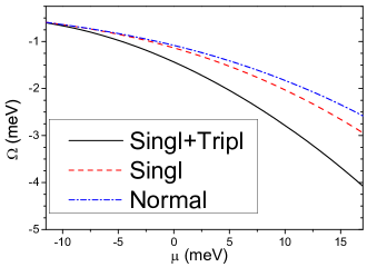
Figure 3: Upper panel: Phase diagram in the plane $U-V$ to distinguish the normal state (absence of superconductivity), singlet, triplet and singlet+triplet (S+P) superconducting phases at the chemical potential $\mu=-9$ meV ( close to the onset of intermediate electronic bands). Lower panel: Comparison between the grand-canonical free energies of the normal state, of the singlet-pairing and the triplet-singlet superconductive ground-states, at $U=350$ meV and $V=600$ meV.

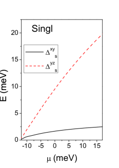
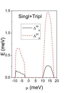
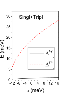
Figure 4: Left panel: Zero temperature singlet pairing amplitudes, for $U=350$ meV and $V=0$ meV. Middle panel: The same as in the left panel, but for $U=350$ meV and $\frac{V}{2}=300$ meV. Right panel: Zero temperature triplet pairing amplitudes, again for $U=350$ meV, $\frac{V}{2}=300$ meV. Notice that, in the absence of magnetic field, $\Delta^{\tau}_{t}=\Delta^{\tau}_{t,\uparrow}=\Delta^{\tau}_{t,\downarrow}$.

By means of our variational procedure, beyond the normal state and a singlet-pairing regime, we find a range of values for $U$ and $V$ where the singlet and triplet pairings coexist. Instead, as pointed out in the previous subsection, no triplet pairing between different spins is found (we will comment later on on this result). When the coexistence takes place, the ratio between $U$ and $V$ can be tuned such that the triplet component of the order parameter is not negligible or even dominant (further details and insight on the solutions described below will be given in Section IV.2, via the analysis of the effective Hamiltonian in Eq. (17)).

First, we focus on the regime of values for $U$ and $V$ where only the singlet pairing is stable. As shown in Fig. 3, this occurs for $U=[300,400]\>{\rm meV}$ and for $V<600$ meV. Superconductivity becomes stable once the chemical potential $\mu$ is set above the minimum of the rotated band $\eta_{0}$, around $-54$ meV. Conversely, no pairing is observed for lower values of $\mu$. As reported in Fig. 3, for $U<300$ meV, superconductivity is not found (that is true at any $\mu$).

In the left panel of Fig. 4, corresponding to $U=350$ meV and $V=0$, we plot the singlet order parameters, showing that they are different from zero, starting from the minimum of intermediate pair of bands ($\mu$ goes from about $-10$ meV to about $20$ meV). The obtained starting point for superconductivity is in agreement with the appearance of a finite density of states, shown in the previous Section, and with the experimentally measured behavior of the superconducting pairing gariglio2016 ; singh . We remark that we always find ${\color[rgb]{0,0,0}\Delta_{s}^{yz}}={\color[rgb]{0,0,0}\Delta_{s}^{zx}}$ in the self-consistent superconducting solutions. Moreover, as shown in the left panel of Fig. 4, not only ${\color[rgb]{0,0,0}\Delta_{s}^{yz}}$, but also ${\color[rgb]{0,0,0}\Delta_{s}^{xy}}$ is different from zero, starting from the the minimum of the $\eta_{0}$ band. Due to the difference of mass and density of states in the normal state, ${\color[rgb]{0,0,0}\Delta_{s}^{xy}}$ is smaller than ${\color[rgb]{0,0,0}\Delta_{s}^{yz}}$. We also point out that, increasing the carrier density, the order parameters get enhanced continuously: apparently, there is no dome, as a function of the density. This finding matches the general result in paramekanti2020 , relating the presence of superconducting domes with finite-range potentials.

Then, we consider the effect of a nonzero attractive term $\propto V$. As reported in Fig. 3, for $V\gg U$, the triplet is the dominant pairing, while the singlet pairing tends to vanish. However, Fig. 3 shows an intermediate regime, from values of $V$ slightly smaller than $2U$, where the order parameters coexist. In the middle panel of Fig. 4, we plot the singlet order parameters for the different orbitals in the same regime, as a function of the chemical potential. At finite $V$, the appearance of a triplet pairing parallels a reduction of the s-wave order parameters. In particular, the smallest one, $\Delta_{s}^{xy}$ assumes values in agreement with experimental estimates, around $0.1$ meV. Therefore, there is a destructive interference between singlet and triplet amplitude pairings. Moreover, this interplay is also able to induce a dome, as a function of the density, beginning from the place where the density of states of the normal phase shows a step. We notice that a similar behavior takes place at higher densities, corresponding to the minimum of the band $\eta_{+}$, where the density of states has another step. Therefore, our theoretical calculation predicts that, beyond the over-doped regime of the first dome, corresponding to the band $\eta_{0}$, there is a possibility of a second dome with similar extent, related to the higher energy band $\eta_{+}$. We observe finally the presence of a regime where $U\neq 0$ and $V\neq 0$ but the normal state is favoured. This effect is due to a low density of states in the analyzed range of chemical potential, much lower (at least two orders of magnitude) than in a standard metal. To rule out the possibility that this would be due to finite-size effects, in our calculation, we analyzed $L\times L$ square lattices up to $L=160$, checking numerical convergence of the superconductive gap parameters. Also a MF analysis on the $\eta_{-}$ and $\eta_{0}$ bands, starting from the effective theory in Eq. (17), led to the same conclusion.

Figure 5: Upper Panel: Relative critical temperature for singlet order parameters, at $U=350$ meV, $\frac{V}{2}=600$ meV, and $\mu$ varying, starting from the bottom of $\eta_{0}$ as calculate in this paper. Lower Panel: Relative critical temperature taken from Ref. Stornaiuolo

Finally, in the right panel of Fig. 4, we plot the $\uparrow$ triplet amplitudes for the orbital $\tau$, again at $U=350$ meV and $\frac{V}{2}=300$ meV. In analogy with the singlet pairing, we always find $\Delta_{t,\sigma}^{yz}=\Delta_{t,\sigma}^{zx}$, therefore the orbital $yz$ and $zx$ are strongly coupled also in the triplet channel. Moreover, since there is no applied magnetic field, $\Delta_{t,\uparrow}^{\tau}=\Delta_{t,\downarrow}^{\tau}$. We notice that the triplet pairings always increase as a function of the density, then the reduction of the singlet pairing is compensated by an enhancement of the triplet channel, for all the values of the chemical potentials.

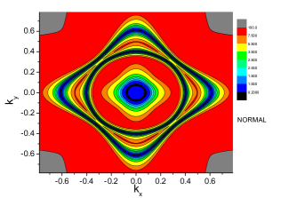
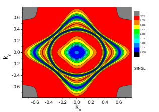
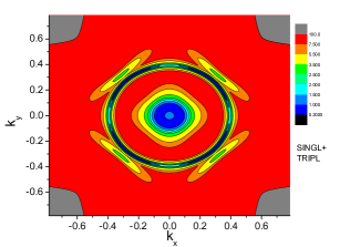
Figure 6: Upper panel: Bogoliubov-de Gennes spectra at $\mu=-9$ meV, for $U=V=0$ meV. Central panel: The same as in the upper panel, but for $U=350$ meV, $V=0$ meV. Lower panel: The same as in th upper panel, but for $U=350$ meV and $\frac{V}{2}=300$ meV.

In the lower panel of Fig. (3), we perform a comparison between the grand-canonical free energies of the normal state, of the singlet-pairing and the triplet-singlet superconductive ground-states, at $U=350$ meV and $V=600$ meV. We point out that the grand-canonical potential can be lowered in a significant way if the triplet component is included in the energy balance.

In Fig. 5 (upper panel), we plot the relative critical temperature for the singlet order parameters, obtained by employing the mean-field approach, and by varying the particle density and by setting $U=350$ meV and $\frac{V}{2}=300$ meV. Moreover, the range for the single-particle energy to starts from the bottom of the $\eta_{0}$ band. We recover a dome-shaped plot, with the maximum critical temperature $T_{c}^{\mathrm{max}}\simeq 1$ K. At this critical temperature, the triplet order parameters are reduced, in comparison to their value at zero temperature, however they are not necessarily zero.

More in detail, we locate the beginning the first dome at energy $E=\mu=-10$ meV and electronic density $n=2.14\cdot 10^{13}$ $\mathrm{cm}^{-}2$, the maximum of $T_{c}$ at E = - 7 meV and $n=2.6\cdot 10^{13}$ $\mathrm{cm}^{-2}$, and finally the end of the first dome at E = -2.5 meV and $n=3.3\cdot 10^{13}$ $\mathrm{cm}^{-2}$. These values can be compared e.g. with experimental data in Stornaiuolo , summed up in the lower panel of Fig. 5. There the same dome is measured between $n=1.8\cdot 10^{13}$ $\mathrm{cm}^{-2}$ and $n=3.1\cdot 10^{13}$ $\mathrm{cm}^{-2}$, the top of the dome being around $n=2.4\cdot 10^{13}$ $\mathrm{cm}^{-}2$. Therefore, we find a reasonable agreement between theory and experiment. We remark that experimental data joshua2012universal ; Stornaiuolo have identified a critical value $n_{c}$ of the density of the order of $1.8-1.9$ $10^{13}$ $\mathrm{cm}^{-2}$, which characterizes the underdoped superconducting regime. Actually, in comparison with experimental results, as reported in Fig. 5, the theoretical data show only a slight shift of the entire phase diagram. In our approach, this effect depends only on the energy $E_{t}$ which measures the energy distance between the band $xy$ and $yz$ in Hamiltonian 5. If a slightly smaller value than 50 meV had been chosen, a perfect agreement with the experimental critical temperature would be obtained.

Since the triplet order parameter depends on the momentum ${\bf k}$, it is interesting to plot the Bogoliubov-de Gennes spectrum obtained by using the superconducting order parameters obtained from the minimization of the free energy $\Omega$. In Fig. 6, we focus onto $\mu=-9$ meV, that is, a chemical potential slightly higher than the minimum of the band $\eta_{0}$. First, in the upper panel of Fig. 6, we plot the spectrum corresponding to the normal state. The zeros correspond to the the center zone $\eta_{0}$ and the finite momentum zone $\eta_{-}$ whose origin is $xy$-like. At finite momentum, there is a small splitting of the zeroes, due to the fact that this value of the chemical potential is close to the avoided crossing of the electronic bands. In the middle panel of Fig. 6, we plot the spectrum corresponding to the singlet pairing. The gaps correspond to the center zone $\eta_{0}$ and the finite momentum zone $\eta_{-}$ whose origin is $xy$-like. Therefore, the gaps at finite momentum are smaller than those at center zone. However, when only the singlet is present, along the $\Gamma X$ ($k_{y}=0$ or $k_{x}=0$) and $\Gamma M$ ($k_{x}=k_{y}$) directions, the gaps are perfectly symmetric. Finally, in the left panel of Fig. 6, we consider the combined effect of singlet and triplet pairings. We notice that the spectrum drastically changes with respect to the case where only the singlet is present. In particular, the gaps get reduced along $\Gamma M$ direction. This behavior can be ascribed to the $s_{x}$ and $s_{y}$ dependence of the order parameter given in Eq. (III.2): along the $\Gamma M$ direction, at finite wave-vector, the gap is mainly given by singlet channel.

To conclude, we mention the interesting possibility to consider possible superconductive solutions from the continuum effective Hamiltonians in Eqs. (16) and (17). We analyzed their presence, by adding an attractive potential as in Eq. (19). Working with lattice sizes up to $L=256$, we found only normal solutions in large ranges for $U$ and $V$ (as large as in Section III). We ascribe this outcome to relevant finite-size effects at the considered low fillings $\nu<0.1$, required for the validities of the effective theories in Eqs. (16) and (17).

IV.2 Clues of emerging topology at zero magnetic field

The pairing in Eq. (III.2), preserving time-reversal invariance, leads to a Bogoliubov Hamiltonian in the class DIII of the classification for topological insulators and superconductors ludwig2009 ; ryu2016 ; Bernevigbook . Indeed $U_{T}={\bf I}_{3\mathrm{x}3}\otimes{\bf I}_{2\mathrm{x}2}\otimes\sigma_{y}$, $U_{T}\,U_{T}^{*}={\bf I}_{12\mathrm{x}12}$ and $U_{C}={\bf I}_{3\mathrm{x}3}\otimes\sigma_{y}\otimes\sigma_{y}$, $U_{C}\,U_{C}^{*}=-{\bf I}_{12\mathrm{x}12}$ (the second matrices in the Kronecker products acting on the Nambu-Gorkov indices). The chiral symmetry $U_{S}=U_{T}\,U_{C}=U_{C}\,U_{T}$, $U_{S}^{2}={\bf I}_{12\mathrm{x}12}$, is also realized, however not affecting the topology class (see Appendix 1). In this class, nontrivial topological configurations are possible. Therefore, in the following we are going to explore this possibility.

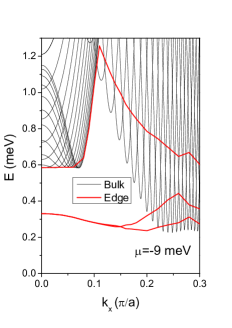
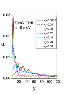
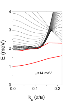
Figure 7: Bogoliubov spectrum for varying $k_{x}$, $U=350$ meV, $V=600$ meV, at $\mu=-9$ meV (first dome) in the left panel, at $U=310$ meV, $V=520$ meV $\mu=14$ meV (second dome) in the right panel. The probability P of the first edge state corresponding to the spectrum of the left panel as a function of the position y (in units of the lattice parameter $a$) for different values of $k_{x}$. For all the plots, a finite size $L_{y}=950$ along the $y$-axis is adopted.

We have analyzed the topological features of the (minimal energy) mean-field superconducting solutions, within the tight-binding scheme exposed in the above. In particular, we have examined different values of chemical potential. Correspondingly, we found signatures of helical superconductivity, both in the first and second dome. As an example, in the left and middle panels of Fig. 7, we show the Bogoliubov spectrum at $\mu=-9$ meV (that is, in the correspondence of the second dome, that means for the $\eta_{0}$ bands), for a lattice that is infinite along the $x$-axis, but is finite along $y$-axis, thus breaking translational invariance in that direction. In particular, along the $y$-axis, we have considered a finite size of $L_{y}=950$ sites, with hard-wall boundary conditions. Then, we have calculated the excitation spectrum at fixed $k_{x}$, finding that two finite-energy edge states are present within the bulk gap, which become degenerate at $k_{x}=0$. This can be ascribed to the fact that, at the onset of the first dome ($\mu\simeq-10$ meV), as shown in Fig. 1, the energy spectrum in the normal state does not present a linear Rashba coupling. Therefore, in the limit of small wave-vectors, the dispersion of the edge states is not linear, as a function of $k_{x}$. Rather, it is nearly flat. As shown in the middle panel of Fig. 7, for small values of $k_{x}$, the wavefunctions corresponding to the in-gap edge states are well localized close to an edge of the system. With increasing $k_{x}$, their wave-function tends to spread over all the bulk.

We point out that the observed behavior is mostly related to the triplet pairing. Indeed, at zero magnetic field, the singlet pairing term alone is not able to provide nontrivial topological phases. However, at $\mu=-9$ meV we have checked a topological phase transition, induced by the attractive term $V$ in Eq. (19) when the triplet order parameters are stable (see Fig. 3). In particular, the results shown in Fig. 7 are obtained when singlet and triplet pairings coexist above a critical value of the attractive potential $V$. In Section IV.3, we discuss in detail the nature of those phase transitions.

We have also analyzed some features, possibly topological, at higher values of the carrier density. In the left panel of Fig. 7, we report the excitation spectrum, with finite size along $y$-axis and at $\mu=14$ meV. Even if the excitation spectrum is more complex in comparison with that shown at lower densities, at zero magnetic field, we still find the presence of in-gap edge states, which gradually merge in the bulk continuum, with increasing $k_{x}$.

IV.3 Further insights from the effective theory

Starting from the full multiband Hamiltonian in Eq. (1), it is rather cumbersome to characterize entirely the full topology content of our system, since it is tough to recover the required analytical form of the band wave-functions in momentum space ludwig2009 ; ryu2016 ; Bernevigbook . However, this task can be achieved, at least partially, starting from the effective Hamiltonians in Eqs. (16) and especially (17). This approaches demonstrates to be valuable also for a better characterization of the entire phase diagram in the considered range of fillings, as well as of the nature of the first superconducting dome.

Since in most of the available literature gariglio2016 , the superconducting dome is located approximately in correspondence of the $\eta_{0}$ band, we focus mainly on $H_{0}^{(\mathrm{eff})}({\bf k})$ in Eqs. (17), with superconducting pairings added. We recall that $H_{0}^{(\mathrm{eff})}({\bf k})$ is expected to described properly at least the lower-density half of the dome. Moreover, the resulting Bogoliubov Hamiltonian shares the same (time-reversal and charge-conjugation) symmetry content as the multiband one in Eq. (20), therefore allowing (but not guaranteeing) the same topological phase structure. Indeed, a similar discussion can be performed directly for the $\tau$ bands, obtaining the same qualitative results: for a given pair content, the effective spin-orbit ${\bf g}({\bf k})$ (absent in the $\tau$ bands basis) has only quantitative effects on the phase diagram.

We assume again a pairing ${\bf\Delta}(\bf{k})$, in the form of Eq. (22) ( at this stage, we do not need to specify the precise form of the corresponding attractive potential, which instead we generically denote as $G$). The resulting Bogoliubov Hamiltonian is of the general form $H_{0}^{\mathrm{BG}}=\frac{1}{2}\sum_{\bf{k}}\psi^{{\dagger}}_{\bf{k}}\mathcal{H}(\bf{k})\psi^{\ }_{\bf{k}}$, with

$$\mathcal{H}(\bf{k})=\left(\begin{array}[]{cc}h_{0}(\bf{k})&{\bf\Delta}(\bf{k})\\ {\bf\Delta}^{{\dagger}}(\bf{k})&-h_{0}^{T}(-\bf{k})\end{array}\right)$$ (25)

$\psi_{\bf{k}}=(c^{\ }_{{\bf k}\uparrow},c^{\ }_{\bf{k}\downarrow}c^{{\dagger}}_{-\bf{k}\uparrow},c^{{\dagger}}_{-\bf{k}\downarrow})^{\mathrm{T}}$ and

$$h_{0}({{\bf k}})=\xi_{0}({\bf k})\,{\bf I}_{2\mathrm{x}2}+{\bf g}({\bf k})\cdot\bm{\sigma}\,.$$ (26)

with $\xi_{0}({\bf k})=\epsilon_{0}({\bf k})-\mu$ ($\mu$ measured from $\epsilon_{0}({\bf k}=0)$). By time-reversal-symmetry, it turns out that $\xi_{0}({\bf k})$ and ${\bf g}({\bf k})$ are symmetric and antisymmetric in ${\bf k}$, respectively sato2006 . The Hamiltonian in Eq. (25) has the spectrum sato2006

$$E_{\pm}({\bf k})=\sqrt{\Big{(}\xi_{0}({\bf k})\pm|{\bf g}({\bf k})|\Big{)}^{2}+\Big{(}\Delta_{s}\pm|{\bf d}({\bf k})|\Big{)}^{2}}$$ (27)

if ${\bf d}({\bf k})$ (see Eq. (22)) is aligned with ${\bf g}({\bf k})$, which is the most likely possibility, as we noted above. In three dimensional systems, this spectrum can give rise to topologically-protected nodal lines, where $E_{-}({\bf k})=0$, leading to nodal (non-centrosymmetric) superconductors. These systems require a partially different topological classification from the ten-fold way for fully gapped ones brydon2015 ; samokhin2015 , as well as for their edge modes samokhin2016 . However, in two dimensions, only isolated zeros for $E_{\pm}({\bf k})=0$ can occur, not topologically protected, and identified as transition points.

We analyze separately three configurations for ${\bf d}({\bf k})$: i) pure s-wave (spin singlet) pairing, ii) pure p-wave (triplet) state, iii) mixed s-p waves pairing. In the first configuration, no topology is realized: the phase is continuously connected with a purely BCS one, where ${\bf g}({\bf k})=0$. Indeed, in spite of ${\bf g}({\bf k})\neq 0$, since $\Delta_{s}\neq 0$, no zeros of $E_{\pm}({\bf k})$ can occur in between and for a certain ${\bf k}$. This regime clearly corresponds to that in Section IV for the multiband model in Eq. (20), at $\mu=-9$ meV, $U<300$ meV and $V=0$.

In the normal state, due to the terms in Eqs. (11) and (13), mixing the spins, only the sum of the spin currents is conserved, related to the global symmetry group $U(1)_{V}$, in turn defined by the transformations: $c_{\uparrow}({\bf k})\to e^{i\theta}\,c_{\uparrow}({\bf k})$, $\theta=[0,2\pi)$, and the same for $c_{\downarrow}({\bf k})$. Therefore, due to the bilinear pairing condensate $\langle c_{\uparrow}({\bf k})c_{\downarrow}(-{\bf k})\rangle=\Delta_{s}$, the spontaneous symmetry breaking

$$U(1)_{V}\to Z_{2\,V}$$ (28)

occurs, where for $Z_{2\,V}\in U(1)_{V}$, $\theta=\{0,\pi\}$.

Similarly, in the configuration ii), when $\Delta_{s}=0$, two phases can be realized a priori, in this scheme discerned by the sign of $\mu$ readgreen ; Bernevigbook . These two phases, one with non trivial and one with trivial topologies, are continuously connected with those at ${\bf g}({\bf k})=0$. This because the unique zeros of $E_{\pm}({\bf k})$ can occur where ${\bf d}({\bf k})=0$, that means at ${\bf k}=0$. In this point, also ${\bf g}({\bf k})=0$ and $\epsilon_{0}({\bf k})=0$, therefore $E_{\pm}({\bf k})=\mu$. Now, as $G\to 0$, then $\mu\approx k_{F}>0$ (since the filling of the $\eta_{0}$ band is positive), while the condition $\mu=0$, separating the two phases, occurs for $G$ large enough (similarly as in the previous Section). Again, the breaking pattern in Eq. (28) is realized.

The data from the mean-field analysis on the lattice suggests that the topological phase sets in for $U\geq 250$ and $V\geq 550$ meV, where we find the triplet pairing (see Fig. 3). The same phase, a superconducting counterpart of a quantum spin Hall phase, is the unique possible topological one in the DIII class and in two dimensions ludwig2009 ; ryu2016 ; Bernevigbook , and it is also known as helical superconducting phase. Moreover, this is labelled by a topological index $n=1$, witnessing the number of pairs of edge states, related by the time-reversal conjugation qi2009 ; Bernevigbook . This index (written for the general case e.g. in sato2017 ) becomes, in the limit of decoupled spin sectors, ${\bf g}({\bf k})\to 0,\,\,\forall\,{\bf k}$, Bernevigbook :

$$n=\frac{1}{2}\,(n_{\uparrow}-n_{\downarrow})\quad\mathrm{mod}\,2\,,$$ (29)

where $n_{\uparrow}=1$ and $n_{\downarrow}=-1$ label the topological phases (with broken time-reversal invariance, then in the D class of the ten-fold way classification ludwig2009 ; ryu2016 ; Bernevigbook ) described in readgreen . The numbers $n_{\uparrow/\downarrow}=\pm 1$ correspond to nontrivial element of the first homotopy class nakahara ; coleman1 ; coleman2 , $\pi_{1}(\tilde{O)}$, on a circle $\tilde{O}$ around the high symmetry node at ${\bf k}=0$. In particular, the nontrivial homotopies are related to the phase factors $e^{\pm i\,\phi_{\bf k}}$ parametrizing as follows the nonvanishing p-wave gaps (connected by time reversal conjugation):

$$\Delta_{t,\uparrow/\downarrow}\,(k_{x}\pm i\,k_{y})=\Delta_{t,\uparrow/\downarrow}\,|{\bf k}|\,e^{\pm i\,\phi_{\bf k}}\,.$$ (30)

Therefore, for instance, $n=0$ for the extended s-wave case, considered in zeg2020 . In the more general case where the spin sectors are coupled together (as when ${\bf g}({\bf k})\neq 0$, or in the presence of a superconducting pairing between the two spin-species, as in the case iii)), the topological index $n=1$ can be expressed in terms of Chern numbers of positive- and negative-energy eigenstates sato2017 . Alternatively, the same index can be defined as a winding number of a phase yokoyama2014 , exploiting directly the full Bogoliubov Hamiltonian $H_{\mathrm{BG}}({\bf k})$, instead of its bands ( see notatop for more details).

Finally, in the configuration iii), where singlet and triplet pairings coexist, a trivial and a topological phase can be again realized a priori. Referring to the Hamiltonian in Eq. (26), they are separated by the condition (on $G$, $\mu$, $\Delta_{s}$, and ${\bf d}({\bf k})$) that $E_{-}({\bf k})=0$, for a certain $|{\bf k}|$. This is expected for $|\Delta_{s}|\sim|\Delta_{t,\uparrow}|=|\Delta_{t,\downarrow}|$. Again, the breaking pattern in Eq. (28) is realized. Being again in the DIII class of the ten-fold way classification, the two phases belong respectively to the same topological classes of the phases in the case ii), then they are discerned by the same topological index yokoyama2014 ; sato2017 .

This situation corresponds to the singlet-triplet coexisting regime, found in Section IV. Correspondingly, the presence of edge states indicates that between the two possible phases described above, the topological one is realized. In the following Section, we will analyze its response to an applied magnetic field.

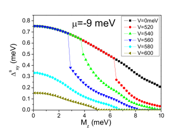
Figure 8: Upper panel: Singlet order parameter $\Delta^{xy}_{s}$, as a function of the magnetic field along the $z$-axis for $U=350$ meV and for different values of the attractive term $V$ and at $\mu=-9$ meV. Lower panel: Same as in the upper panel, but with the magnetic field along the $x$-axis (lower panel). We recall that in Eq. (19) the nearest neighbour pairing has coupling $\frac{V}{2}$.

V Superconducting solutions in the presence of a magnetic field

It is important, on the experimental point of view as well, to consider how the above scenario is modified under the application of a uniform magnetic field, inducing the Zeeman term in Eq. (14). For this purpose, we start with discussing how an applied magnetic field modifies the superconducting order parameter.

V.1 Effects of the magnetic field on the superconducting order parameter

The first macroscopic effect is the breakdown of the time-reversal symmetry. Along this direction, we analyze the effects of an external magnetic field on the superconducting solutions, considering field orientations both along the $z$-axis (out-plane) and the $x$-axis (in-plane).

First, we focus on the singlet order parameter related to the orbital $xy$, $\Delta_{xy}^{s}$. We recall that this order parameter provides an estimate of the minimal superconducting gap in the excitation spectrum. In the upper panel of Fig. 8, we plot this quantity, as a function of $M_{x}$, and for different values of $V$. In particular, we focus on the under-doped regime of the first dome, at $\mu=-9$ meV. For $V=0$, there is a continuous curve, as a function of the magnetic field. However, there is a range of values for $V$ where the order parameter shows a discontinuity. Actually, this discontinuity marks the onset of the triplet pairing, which, on the other hand, start weakening the singlet order parameter (see Fig. 3). As shown below, the triplet pairing can lower the ground-state energy, at increasing magnetic field and fixed $V$. Therefore, there is a transition between a phase with only the singlet pairing to a phase with combined singlet and triplet pairings. With increasing $V$, the triplet pairing becomes stable at lower strengths of the magnetic field (Indeed, we have shown above that, for $V>560$ meV, there is the formation of the triplet pairing even at $M_{z}=0$). For these values of $V$, the reduction of the singlet order parameter is quite rapid as a function of the strength of $M_{z}$.

In the lower panel of Fig. 8, we plot $\Delta_{xy}^{s}$ as a function of $M_{x}$, for different values of $V$. There is a different coupling between the in-plane magnetic field and the triplet order parameter. Therefore, the role of the triplet pairing is affected not only by the density, but also by the orientation of the magnetic field. Indeed, it can be responsible of the experimentally measured magnetic field anisotropy, in some superconducting properties, between the in-plane and out-of-plane field configurations caviglia2009 . In particular, in the under-doped regime of the first dome, at $\mu=-9$ meV, the anisotropy emerging from the comparison between the upper and lower panels of Fig. 8 is present but not marked. Indeed, the behavior of the order parameter, as a function of $M_{x}$, follows that as a function of $M_{z}$, the first behavior being characterized only by slightly smaller values of critical fields (at different $V$).

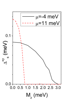
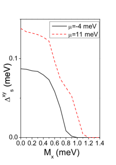
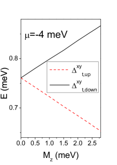
Figure 9: Singlet (left panel) and triplet (right panel) pairing amplitudes, as a function of a constant magnetic field ${\bf M}$ along the $z$-axis (out of plane) with $U=350$ meV and $\frac{V}{2}=300$ meV. Middle panel: same as in the left panel, but with the magnetic field along $x$-axis (in-plane).

In order to deeply analyze the role of the anisotropy of the superconducting solutions, we consider different fillings, comparing the behaviors of the order parameters between the first dome, beginning at the minimum of the $\eta_{0}$ band ($\mu\approx-10$ meV), and the second one, related to the $\eta_{+}$ band ($\mu\approx 10$ meV). Therefore, in the left and the middle panel of Fig. 9, we consider two values of $\mu$: $\mu=-4$ meV, corresponding to the over-doped regime of the first dome, and $\mu=-11$ meV, corresponding to the under-doped regime of the second dome. In the left panel we analyze the behavior of $\Delta_{xy}^{s}$, as a function of $M_{z}$, and in the middle panel we draw a similar plot, evidencing the dependence on $M_{x}$. Actually, as shown in Fig. 9, at $\mu=-4$ meV, there is an anisotropy favoring the stability along the $z$-axis. O n the other hand, as discussed above, the triplet pairing becomes stronger with increasing density, and it systematically weakens the singlet amplitudes. Moreover, the triplet order parameters are more sensitive to the magnetic field along the $z$-axis (as shown in the right panel of Fig. 9) than to the one along the $x$-axis. Therefore, with increasing density, the anisotropy changes drastically. In particular, at $\mu=11$ meV, the critical field along $z$ is less than 1 meV, while that along $x$ becomes larger than unity. Therefore, the results are in qualitative agreement with experimental data, caviglia2009 where the anisotropy is more marked. Indeed, even if the role of the triplet pairing can be relevant to inducing anisotropy in the superconducting order parameters, it is not enough to explain all the relevant features found in LAO/STO-001 as a function of in-plane and out-of-plane magnetic fields.

Finally, in the right panel of Fig. 9, we have carefully analyzed also the behavior of the triplet pairing, as a function of $M_{z}$, finding a remarkable linear dependence of the triplet order parameters, opposite for the two spin components: one is enforced, the other one is weakened.

V.2 Clues of emergent topology in the presence of a magnetic field

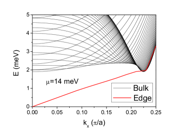
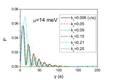
Figure 10: Upper panel: Bogoliubov spectrum for varying $k_{x}$, $V=0$ meV, $\mu=14$ meV and finite size $L_{y}=950$ sites along the $y$-axis. Lower panel: probability of the edge state as a function of the position (in units of the lattice parameter $a$) for different values of $k_{x}$ (in units of $\pi/a$). The value of $M_{z}$, inducing a topological phase transition (see the main text), is smaller than the critical value suppressing the self-consistent superconducting solutions.

We now focus on the possibility of topology in the presence of a magnetic field. In these conditions, the breakdown of the time-reversal symmetry makes the topology class of the system to change from DIII to D. In two dimensions, the latter class still allows nontrivial topology, still labelled by a $Z$ index ($Z_{2}$ for 1D systems; in this case the precise calculation of the related invariant has been performed in perroni2019 ). In this way, a magnetic field can preserve the edge states that we discuss in Section IV.2.

Still analyzing the possible presence of edge states, we find that topological properties are favored by an out-of-plane magnetic field, but disfavored by an in-plane one. Indeed, they are weakened with changing the orientation of the magnetic field from the $z$-axis to $x$-axis, and there here are characteristic angles (around $\frac{\pi}{4}$) where a topological phase transition takes place. Eventually, for a sufficiently intense in-plane magnetic field, one only gets trivial topological phases, in agreement with Loder .

In order to detect the chiral topological superconducting phase when $M_{x}$ is sub-relevant, we consider again a lattice with a finite size along the $y$-axis. In this case, the increase of $M_{z}$ is able to induce a phase transition, as soon as it takes a value of the order of the chemical potential, as measured from the bottom of the sub-band: $M_{z}>\sqrt{\tilde{\mu}^{2}+\Delta^{2}}$, where $\tilde{\mu}$ is the chemical potential measure from the bottom of the $\eta_{+}$ sub-bands, and $\Delta$ is the effective superconductive gap. Thus, the critical values to enter the topological phase depend in general on $U$, $V$, and $\mu$. In the upper and lower panels of Fig. 10, we show the results obtained at $V=0$, with only the singlet pairing present. We remark that, in contrast with the results of the previous Section at zero magnetic field, now the topological phases can be driven by the singlet order parameters only. We find that the chiral Majorana edge states have a linear dispersion as a function of $k_{x}$, and are quite localized at the edge for small values of $k_{x}$, similarly as in Loder . As usual, with increasing $k_{x}$, these states merge into the bulk continuum.

Again the described picture can be understood in better qualitative details by analyzing the effective Hamiltonians in Eqs. (16) and (17), in analogy with the discussion at ${\bf M}=0$ in Section III.1. Since the Zeeman term in Eq. (14) has the form $H_{M}={\bf I}_{3\mathrm{x}3}\otimes{\bf M}\cdot{\bf\sigma}$, it is sufficient to add this term to $H_{0}^{(\mathrm{eff})}$, as described in the Appendix 3 (before Eq. (4)), in spite of the fact that the $zx$ and $yz$ bands are mixed to yield the $\eta_{0}$ band: this mixing is diagonal on the spin $\sigma$ index. In Eq. (26), the same added term results in the shift ${\bf g}({\bf k})\to{\bf g}({\bf k})+{\bf M}$, losing explicitly the antisymmetry required by time-reversal invariance sato2006 .

A Zeeman term, $H^{(z)}_{M}=M_{z}\sigma_{z}$, along the $z$-axis, orthogonal to the plane of our system, creates an effective unbalance in the chemical potentials with respect to $\sigma$. This imbalance is known to spoil the s-wave pairing $\Delta^{\tau}_{s}$ (as well as $\Delta^{\tau}_{p,\uparrow\downarrow}$, if present), leading to the normal phase, or at most to a normal-superconductive mixed one (a secondary possibility that we neglect, in the light of the stability of the p-wave pairing, see below) pethick ; marchetti2007 ; rad2007 . This transition occurs, in the low-pairing limit, around the value $M_{z}=\frac{\mu_{\uparrow}-\mu_{\downarrow}}{2}=\frac{\Delta^{\tau}_{s}}{\sqrt{2}}$, the so called Chandrasekhar-Clogston limit (strictly valid for perturbative Hubbard attractions) pethick . Concerning the triplet pairings $\Delta_{t,\uparrow}$ and $\Delta_{t,\downarrow}$, they are spoiled asymmetrically by the $M_{z}$ term, mainly via the shift of the chemical potentials $\mu_{\uparrow,\downarrow}$. In particular, if $M_{z}>0$, $\mu_{\downarrow}$ is decreased (at fixed $\Delta_{t,\downarrow}$). At a critical value of $M_{z}$, the condition $\mu_{\downarrow}=0$ is realized. Then, the topological phase with $n_{\downarrow}=-1$ is driven to a topologically trivial phase, still with p-wave pairing (the strongly-coupled phase in readgreen ). At the point $\mu_{\downarrow}=0$, a zero in the Bogoliubov gap is reached. The residual topology from the $\uparrow$ contribution is encoded in the $n_{\uparrow}=1\in Z$ phase, belonging to the D class of the ten-fold way classification.

A qualitatively similar phase evolution, determined by the effective unbalances induced by $M_{z}$, is valid if the phases do not host a nontrivial topology, a possibility allowed by symmetry considerations only, and possibly occurring in certain coupling regions, as mentioned in Section IV.2.

VI Conclusions and outlook

In this paper we have discussed the onset and the physical consequences of a singlet-triplet pairing in the two dimensional electron gas at LAO/STO-001 interfaces. This configuration looks rather natural a priori, due to the inversion symmetry breaking term in the tight-binding Hamiltonian of the system. We have made an extended superconducting mean-field analysis of this multi-band tight-binding Hamiltonian, as well as of effective electronic bands in the limit of low values of the momentum. We have included static on-site (favoring spin-singlet pairings) and inter-site (promoting spin-triplet order parameters) intra-band attractive potentials under applied magnetic fields. It is interesting to notice that a singlet-triplet mixed pairing here results robust for extended regions of the analyzed space of parameters.

We have found various interesting features, as a reduction of the singlet order parameter, as a function of the charge density, an asymmetric response to in-plane and out-of-plane magnetic fields (a fact already observed experimentally caviglia2009 ), and the possibility on nontrivial topology and protected edge states. In particular, not-linear spin-orbit couplings and inter-site attractive interactions make stable a time-reversal invariant topological helical superconducting phase in the absence of a magnetic field.

In this paper, we have discussed the interplay between singlet and triplet order pairings in the the clean limit. Effects of dilute nonmagnetic impurities can affect the properties of non-centrosymmetric superconductors samokhin . For example, the impurity effects on the critical temperature are similar to those in multi-band centrosymmetric superconductors. Moreover, Anderson’s theorem holds for singlet pairing samokhin ; anderson1959 . Indeed, we expect that disorder effects can induce a reduction of the triplet order parameters changing only quantitatively the interplay between singlet and triplet pairings. This is the reason why in the paper the focus has been on the properties related to the singlet order parameters.

A natural development of the present work is the study of the effective shape of the dome, that means the finite-temperature dependence. We mention here that we also performed mean-field calculations at finite temperature, finding a first dome for the singlet order parameter, corresponding with the $\eta_{0}$ band, and with a shape qualitatively very similar to that reported in gariglio2016 . However, to achieve reliable quantitative details, the inclusion of fluctuations beyond mean field is required. On the same regard, we also mention a very recent paper jouan2021 , where two-different purely $s$-wave phases have been predicted around the optimal doping, where the critical temperature is maximized. The relation with the present work surely deserves future attention. Other future generalizations of the present work are aimed to include the effect of the second term on the multiband potential in Eq. (18), that is inter-orbital attractive potentials. Closely related, a relevant issue consists of the possibility of nonzero-momentum superconductive couplings between different $\eta$ bands. This feature extremely unlikely in translational invariant systems pethick ; marchetti2007 ; rad2007 , is known to be more stable in lattice systems, see e. g. moore2012 ; shi2013 ; mannarelli2018 .

Finally, we point out that effects due to unconventional superconductivity can be confirmed not only by thermodynamic properties but also by response properties such as the I-V characteristics of Josephson junctions tafuri2017 ; alidoust2021 . In quasi one-dimensional systems, notable properties can be deduced from anomalous Josephson effects tagliacozzo2015 ; tagliacozzo2018 and local spectroscopic measurements perroni_1d . These probes could be also used to disentangle superconducting topological features from trivial ones in the actual two dimensional case.

APPENDIX 1: Hamiltonian symmetries

In this Appendix, we discuss the symmetries of the normal Hamiltonians in Eqs. (3) and (17), as well as the corresponding Bogoliubov Hamiltonians with the pairing in Eq. (III.2) added.

The normal Hamiltonians in Eqs. (3) (here considered at vanishing Zeeman coupling $H_{M}$) can be expressed in terms of Gell-Mann matrices $\{\lambda_{i}\}$, acting on the on the $\tau$ index, times the Pauli matrices acting on the spin index $\sigma$:

$$\Big{(}a({\bf k})\,{\bf I}_{3\mathrm{x}3}+b({\bf k})\,\lambda_{3}+c({\bf k})\,\lambda_{8}\Big{)}\otimes{\bf I}_{2\mathrm{x}2}+w_{\mathrm{SO}}\,\Big{(}-\lambda_{2}\otimes\sigma_{z}+\lambda_{5}\otimes\sigma_{y}-\lambda_{7}\otimes\sigma_{x}\Big{)}+\gamma\,\Big{(}\sin k_{x}\,\lambda_{5}\otimes{\bf I}_{2\mathrm{x}2}+\sin k_{y}\,\lambda_{5}\otimes{\bf I}_{2\mathrm{x}2}\Big{)}\,,$$ (31)

the precise expressions for $a({\bf k})$, $b({\bf k})$, and $c({\bf k})$ being unimportant here. Exploiting now the property for the Pauli matrices, $\{\sigma_{i},\sigma_{j}\}=\delta_{ij}$, it is know immediate to prove (Eq. (15)):

$$H({\bf k})=U_{T}^{-1}H^{*}(-{\bf k})U_{T}\,,\quad\quad\quad U_{T}={\bf I}_{3\mathrm{x}3}\otimes\sigma_{y}\,.$$ (32)

In the Nambu-Gorkov basis $\Psi({\bf k})=\left(\begin{array}[]{c}{\bf c}({\bf k})\\ i\sigma_{y}\,{\bf c}^{\dagger}(-{\bf k})\end{array}\right)$, $c({\bf k})=\left(\begin{array}[]{c}c_{\uparrow}({\bf k})\\ c_{\downarrow}({\bf k})\end{array}\right)$, $H({\bf k})$ is recast as follows:

$$H({\bf k})\to H_{\mathrm{BG}}({\bf k})=\left(\begin{array}[]{cc}H({\bf k})&{\bf 0}_{2\,\mathrm{x}\,2}\\ {\bf 0}_{2\,\mathrm{x}\,2}&-H(-{\bf k})\end{array}\right)$$ (33)

so that $U_{T}$ becomes $U_{T}={\bf I}_{3\mathrm{x}3}\otimes{\bf I}_{2\mathrm{x}2}\otimes\sigma_{y}$, the second identity in the Kronecker product acting on the Nambu-Gorkov indices. The normal effective Hamiltonian in Eq. (17) for the $\eta_{0}$ band, neglecting the out-of-diagonal contribution with higher momentum power than one, reads (see the derivation in the Appendix 3):

$$H_{0}^{(\mathrm{eff})}({\bf k})=\Big{(}-10.8+157.2\,(k_{x}^{2}+k_{y}^{2})\Big{)}\,{\bf I}_{2\mathrm{x}2}-a_{3}\,k_{x}\,\sigma_{y}+a_{3}\,k_{y}\,\sigma_{x}\,.$$ (34)

with $\epsilon_{0}({\bf k})=\big{(}-10.8+157.2\,(k_{x}^{2}+k_{y}^{2})\big{)}$ meV (so that $t_{0}^{(\mathrm{eff})}=157.2$ meV) and $a_{3}=0.8$ meV. It holds:

$$H_{0}^{(\mathrm{eff})}({\bf k})=\tilde{U}_{T}^{-1}H_{0}^{(\mathrm{eff})*}(-{\bf k})\tilde{U}_{T}\,,\quad\quad\quad\tilde{U}_{T}=\sigma_{y}\,,$$ (35)

$\tilde{U}_{T}=\sigma_{y}$ acting on the spin index, as $\sigma_{y}$ in Eq. (32). In the Bogoliubov form, obtained as above for $H({\bf k})$, $\tilde{U}_{T}={\bf I}_{2\mathrm{x}2}\otimes\sigma_{y}$.

The next step is to include the pairing in Eqs. (22) and (III.2). We have to consider the three spin channels:

$$\langle c^{\tau}_{\downarrow}({\bf k})c^{\tau}_{\downarrow}(-{\bf k})\rangle=e^{i\,\phi^{\tau}_{\downarrow\downarrow}}\,{\color[rgb]{0,0,0}\Delta_{t,\downarrow}^{\tau}}(k_{x}-i\,k_{y})\,,$$ (36)

$$\langle c^{\tau}_{\uparrow}({\bf k})c^{\tau}_{\uparrow}(-{\bf k})\rangle=e^{i\,\phi^{\tau}_{\uparrow\uparrow}}\,{\color[rgb]{0,0,0}\Delta_{t,\uparrow}^{\tau}}(k_{x}+i\,k_{y})\,,$$ (37)

and

$$\langle c^{\tau}_{\uparrow}({\bf k})c^{\tau}_{\downarrow}(-{\bf k})\rangle=e^{i\,\phi^{\tau}_{\uparrow\downarrow}}\,\Big{(}{\color[rgb]{0,0,0}\Delta_{s,\uparrow}^{\tau}+\Delta_{t,\uparrow}^{\tau}}\Big{[}\alpha\,(k_{x}+i\,k_{y})+\beta\,(k_{x}-i\,k_{y})\Big{]}\Big{)}\,.$$ (38)

Two global phase factors between $e^{i\,\phi^{\tau}_{\uparrow\downarrow}}$, $e^{i\,\phi^{\tau}_{\uparrow\uparrow}}$, and $e^{i\,\phi^{\tau}_{\downarrow\downarrow}}$ can be reabsorbed overall via a phase redefinition of the fermionic annihilation operators. However, even in this way the third phase cannot be reabsorbed. This phenomenon a condensed matter counterpart to (minimal model for) the CP$\sim$T violation in particle physics, via chiral fermion condensation weinberg2 . We choose to keep the phase factor $e^{i\,\phi^{\tau}_{\uparrow\downarrow}}$.

We notice that time-reversal invariance, interchanging the spins, imposes $\Delta_{t,\uparrow}^{\tau}=\Delta_{t,\downarrow}^{\tau}$, a result also found by the minimization procedure of the mean-field free energy in the main text. Dividing all the parameters in Eq. (38) in real an imaginary parts, it is useful to parametrize them as follows:

$$\langle c^{\tau}_{\uparrow}({\bf k})c^{\tau}_{\downarrow}(-{\bf k})\rangle=\Big{(}\Delta_{1}^{\tau}+i\,\Delta_{2}^{\tau}\Big{)}+\Big{(}\Delta_{3}^{\tau}+i\,\Delta_{4}^{\tau}\Big{)}k_{x}+\Big{(}\Delta_{5}^{\tau}+i\,\Delta_{6}^{\tau}\Big{)}k_{y}\,.$$ (39)

Therefore, for each $\tau$ band, we obtain for the $4\,\mathrm{x}\,4$ pairing block Hamiltonian $H^{\tau}_{{\bf\Delta}}({\bf k})$ of the total one $H_{{\bf\Delta}}({\bf k})$:

$$H^{\tau}_{{\bf\Delta}}({\bf k})=\Delta_{1}^{\tau}\,\big{(}\sigma_{x}\otimes{\bf I}_{2\mathrm{x}2}\big{)}+\Delta_{2}^{\tau}\,\big{(}\sigma_{y}\otimes{\bf I}_{2\mathrm{x}2}\big{)}+\Big{(}\Delta_{1}^{\tau}\,k_{x}+\Delta_{1}^{\tau}\,k_{y}\Big{)}\,\big{(}\sigma_{x}\otimes\sigma_{z}\big{)}-\Big{(}\Delta_{2}^{\tau}\,k_{x}+\Delta_{4}^{\tau}\,k_{y}\Big{)}\,\big{(}\sigma_{y}\otimes\sigma_{x}\big{)}\,.$$ (40)

Imposing now time reversal invariance of the total multiband Hamiltonian $H_{\mathrm{BG}}({\bf k})+H_{{\bf\Delta}}({\bf k})$ (see Eq. (33)),

$$H_{\mathrm{BG}}({\bf k})+H_{{\bf\Delta}}({\bf k})=V_{T}^{-1}\big{(}H^{*}_{\mathrm{BG}}(-{\bf k})+H^{*}_{{\bf\Delta}}(-{\bf k})\big{)}V_{T}\,,$$ (41)

we immediately obtain that it must hold

$$V_{T}=U_{T}={\bf I}_{3\mathrm{x}3}\otimes{\bf I}_{2\mathrm{x}2}\otimes\sigma_{y}\,,$$ (42)

and importantly $\Delta_{2}=\Delta_{4}=\Delta_{6}=0$. That means that all the pairing couplings in Eqs. (36)-(38) must be real, as claimed in the main text. At this point is straightforward to obtain that $H_{\mathrm{BG}}({\bf k})+H^{\tau}_{{\bf\Delta}}({\bf k})$ is also invariant under charge conjugation:

$$H_{\mathrm{BG}}({\bf k})+H_{{\bf\Delta}}({\bf k})=-U_{C}^{-1}\big{(}H^{*}_{\mathrm{BG}}(-{\bf k})+H^{*}_{{\bf\Delta}}(-{\bf k})\big{)}U_{C}\,,\quad\quad{\mathrm{with}}\quad\quad U_{C}={\bf I}_{3\mathrm{x}3}\otimes\sigma_{y}\otimes\sigma_{y}\,.$$ (43)

A further symmetry of the Bogoliubov Hamiltonian $\big{(}H_{\mathrm{BG}}({\bf k})+H_{{\bf\Delta}}({\bf k})\big{)}$ is the chiral symmetry

$$H_{\mathrm{BG}}({\bf k})+H_{{\bf\Delta}}({\bf k})=U_{S}^{-1}\big{(}H^{*}_{\mathrm{BG}}(-{\bf k})+H^{*}_{{\bf\Delta}}(-{\bf k})\big{)}U_{S}\,,\quad\quad U_{S}=U_{T}\,U_{C}=U_{C}\,U_{T}\,,\quad\quad U_{S}^{2}={\bf I}_{12\mathrm{x}12}\,,$$ (44)

composed by the product of time- and charge-conjugation symmetries. Chiral symmetry does not change the topology class of the Bogoliubov Hamiltonian, remaining DIII.

APPENDIX 2: setting the pairing ansatz

On a general lattice, the mean field approach to superconductivity proceeds identifying all the possible pairings corresponding to the irreducible representations of the point-group symmetry of the lattice: the ansatzs for the pairings are expressed in terms of them annett . This procedure is analogous to the expansion in terms of spherical harmonics in the isotropic, $SO(3)$ invariant, free space.

The spectra in Eq. (5), in the absence of the spin-orbit and inversion terms in Eqs. (11) and (13), display a $D_{2}$ point group symmetry dress_book . However, due to the presence of the latter two terms, in order to implement the mean field approach, we have still to assume all the pairings allowed by the symmetry of the isotropic square lattice. This lattice has (finite) point group symmetry $D_{4}$, containing $D_{2}$ and composed by the group $C_{4}$ of the rotation of angles $\theta_{n}=n\,\frac{\pi}{2},\,\,n=0,\dots,3$, and by the reflections around one (vertical or horizontal) axes (see e.g. dress_book ).

In this case, the basis functions labelling the irreducible representations which the eight-fold regular representation decomposes in, are $k_{x}^{2}+k_{y}^{2}$, $k_{x}^{2}-k_{y}^{2}$, $k_{x}k_{y}$, $\Big{(}\begin{array}[]{c}k_{x}\\ k_{y}\end{array}\Big{)}$. The first three (parity even) functions, together with the constant $c$, can be assumed as a basis for the spin-singlet pairings, while the (parity odd) doublet can be assumed as a basis for the spin-triplet pairing. Summing up, the superfluid pairing can be generally assumed as:

$$\Delta=\Delta_{s,0}+\Delta_{s,1}\,m(|{\bf k}|)+\Delta_{s,2}\,f(|{\bf k}|)\,\frac{k_{x}^{2}-k_{y}^{2}}{|{\bf k}|^{2}}+\Delta_{s,3}\,g(|{\bf k}|)\,\hat{k}_{x}\hat{k}_{y}+{\color[rgb]{0,0,0}\Delta_{t}}\,h(|{\bf k}|)\,(\hat{k}_{x}+i\hat{k}_{y})\,,$$ (45)

plus possible powers of these terms (required e. g. in the presence of a strong cubic Rashba-coupling, as in nakamura2012 ). Notice however that pairings involving higher powers than 1 should be less relevant around $k_{x}=k_{y}=0$. Both in the effective theories for $\epsilon_{-}$ and $\epsilon_{0}$ bands, it is expected that the spin-orbit interaction (including the relevant not-linear corrections) plays a critical role in determining the pairings that set in. The effect of a linear spin-orbit coupling has been studied in rashba2001 , where a mixing (singlet-triplet and s-p wave) has been identified. The same situation could be expected here. However, the not-linear spin-orbit couplings could change the picture.

APPENDIX 3: derivation of the effective theories in Eqs. (16) and (17)

In order to probe the presence of non-BCS pairings, suggested by recent works, it is useful to restart considering the structure of the $\epsilon_{yz}$, $\epsilon_{zx}$, and $\epsilon_{xy}$ bands (in the absence of Zeeman couplings), as well as the real bands $\epsilon_{+,i}$, $\epsilon_{0,i}$, and $\epsilon_{-,i}$ (in the following we will neglect the degeneracy index $i$, for sake of brevity) resulting from the mixing of them, according to the Hamiltonian in Eq. (3). The plots of them are given in Fig. 1.

It is clear that the mixing of the $\epsilon_{yz}$, $\epsilon_{zx}$, and $\epsilon_{xy}$ is relevant only around their band-touching points, around the momenta $k_{x}=k_{y}=0$ and $k_{x}=k_{0}\approx\pm 0.35,k_{y}=0$, as expected from the low ratios $\frac{\gamma}{t_{1}}$ and $\frac{\Delta_{so}}{t_{1}}$ in Eq. (3). Clearly, the importance of the same mixing relatively to the three bands depends on which ones are touching each others: around $k_{x}=0$, the bands $\epsilon_{yz}$, $\epsilon_{zx}$ undergo an important mixing, while around the point $k_{x}=k_{0},k_{y}=0$ ($k_{x}=0,k_{y}\approx\pm 0.35$), the bands $\epsilon_{zx}$, and $\epsilon_{xy}$ ($\epsilon_{yz}$, and $\epsilon_{xy}$) do.

We focus first around the point $k_{x}=k_{y}=0$. In this region, due to the relatively small ratios $\lambda_{1}=\frac{\gamma}{{\color[rgb]{0,0,0}E_{t}}}=0.4$ and $\lambda_{2}=\frac{\Delta_{so}}{{\color[rgb]{0,0,0}E_{t}}}=0.2$ effective expressions can be obtained for $\epsilon_{+}$, $\epsilon_{0}$, and $\epsilon_{-}$, exploiting second-order perturbation theory (in standard notation):

$$E_{n}(\lambda)=E_{n}^{(0)}+\lambda^{2}\sum_{k\neq n}\frac{|\langle k^{(0)}|V|n^{(0)}\rangle|^{2}}{E_{n}^{(0)}-E_{k}^{(0)}}+O(\lambda^{3})\,,$$ (46)

and, in the presence of two perturbations $\lambda_{1}\,V_{1}$ and $\lambda_{2}\,V_{2}$:

$$E_{n}(\lambda)=E_{n}^{(0)}+{\color[rgb]{0,0,0}E_{t}}^{2}\,\sum_{i}\lambda_{i}^{2}\sum_{k\neq n}\frac{|\langle k^{(0)}|V_{i}|n^{(0)}\rangle|^{2}}{E_{n}^{(0)}-E_{k}^{(0)}}+{\color[rgb]{0,0,0}E_{t}}^{2}\,\lambda_{1}\lambda_{2}\,\sum_{k\neq n}\Bigg{(}\frac{\langle k^{(0)}|V_{1}|n^{(0)}\rangle\langle n^{(0)}|V_{2}|k_{0}^{(0)}\rangle}{E_{n}^{(0)}-E_{k}^{(0)}}+\mathrm{H.c.}\Bigg{)}+O(\lambda^{3})\,.$$ (47)

Lower band

We start with the derivation of the effective theory for the $\eta_{-}$ band. Exploiting Eq. (47), the couplings of $\epsilon_{xy}$ with $\epsilon_{yz}$ and $\epsilon_{zx}$, included perturbatively, yields to

$$H_{-}^{(\mathrm{eff})}=\Big{(}\epsilon_{xy}+{\color[rgb]{0,0,0}E_{t}}^{2}\,\frac{\lambda_{1}^{2}\sin^{2}k_{x}+\lambda_{2}^{2}}{\epsilon_{xy}-\epsilon_{yz}}+{\color[rgb]{0,0,0}E_{t}}^{2}\,\frac{\lambda_{1}^{2}\sin^{2}k_{y}+\lambda_{2}^{2}}{\epsilon_{xy}-\epsilon_{zx}}\Big{)}\,{\bf I}+2\,{\color[rgb]{0,0,0}E_{t}}^{2}\,\lambda_{1}\,\lambda_{2}\,\Big{(}\frac{\sigma_{y}\sin k_{x}}{\epsilon_{xy}-\epsilon_{yz}}-\frac{\sigma_{x}\sin k_{y}}{\epsilon_{xy}-\epsilon_{zx}}\Big{)}+O(\lambda_{i}^{3})\,,$$ (48)

and, expanding in powers of $k_{x}$ and $k_{y}$:

$$H_{-}^{(\mathrm{eff})}({\bf k})=\epsilon_{-}({\bf k})\,{\bf I}-(a_{1}\,k_{x}+a_{2}\,k_{x}^{3})\,\sigma_{y}+(a_{1}\,k_{y}+a_{2}\,k_{y}^{3})\,\sigma_{x}\,,$$ (49)

with $a_{1}=8$ meV (in units of the lattice step $a\equiv 1$), $a_{2}=43.46$ meV, $\epsilon_{-}({\bf k})=\big{(}-54.+280.8\,(k_{x}^{2}+k_{y}^{2})\big{)}$ meV (so that $t_{-}^{(\mathrm{eff})}=280.8$ meV). The spectrum of the effective Hamiltonian in Eq. (49), compared with the exact one, is shown in Fig. 11. The agreement is excellent around $k_{x}=k_{y}=0$.

Central band

The derivation of the effective theory for the $\eta_{0}$ band is more subtle. Indeed, the $\epsilon_{yz}$, $\epsilon_{zx}$ are degenerate at $k_{x}=k_{y}=0$, then before applying second-order perturbation theory, some elaboration of the Hamiltonian (3) is required. In particular, we notice that $H_{Z}({\bf k})$ in Eq. (13) do not mix $\epsilon_{zx}$ with $\epsilon_{yz}$. Therefore we start diagonalizing exactly the partial Hamiltonian $H_{0}({\bf k})+H_{SO}$ in the subspace $\epsilon_{zx}$ with $\epsilon_{yz}$, by a unitary transformation $O=\mathrm{diag}(O_{2\mathrm{x}2},1)$). This transformation does not mix the spins, therefore $O$ can ne also written as $O=\tilde{O}_{2\mathrm{x}2}\otimes{\bf I}_{2\mathrm{x}2}$. In this way, we obtain

$$H_{0}^{\prime}+H_{SO}^{\prime\,(\mathrm{rid})}=\left[\begin{array}[]{ccc}\epsilon_{a}\,{\bf I}&{\bf 0}&{\bf 0}\\ {\bf 0}&\epsilon_{b}\,{\bf I}&{\bf 0}\\ {\bf 0}&{\bf 0}&\epsilon_{xy}\,{\bf I}\end{array}\right]\;\;\;\;,$$ (50)

with $\epsilon_{a}<\epsilon_{b}$ around $k_{x}=k_{y}=0$. At this level, the spins get mixed each others. The bands $\epsilon_{a}$, $\epsilon_{b}$, and $\epsilon_{xy}$ are coupled further by the terms from $H_{SO}$ and $H_{Z}({\bf k})$, rotated by $O$:

$$H_{0}^{\prime}+H_{SO}^{\prime}+H^{\prime}_{Z}=\left[\begin{array}[]{ccc}\epsilon_{a}\,{\bf I}&{\bf 0}&V\\ {\bf 0}&\epsilon_{b}\,{\bf I}&W\\ V^{\dagger}&W^{\dagger}&\epsilon_{xy}\,{\bf I}\end{array}\right]\,,$$ (51)

where

$$V({\bf k})\equiv V=\left[\begin{array}[]{cc}a({\bf k})&b({\bf k})\\ {}\hfil\\ -b^{*}({\bf k})&a({\bf k})\\ \end{array}\right]$$ (52)

is the matrix mixing the $\epsilon_{a}$ and $\epsilon_{xy}$ bands, while $W$ is the matrix mixing $\epsilon_{b}$ and $\epsilon_{xy}$. The precise expressions for its elements are rather involved and not immediately relevant here. No further coupling between $\epsilon_{b}$ and $\epsilon_{a}$ occurs from $H_{SO}$ and $H_{Z}({\bf k})$.

The effect of $V$ and $W$ is introduced perturbatively, as above, obtaining for $\epsilon_{a}$:

$$H_{0}^{(\mathrm{eff})}=\epsilon_{a}\,{\bf I}+\frac{1}{\epsilon_{a}-\epsilon_{xy}}\,\left[\begin{array}[]{cc}|a({\bf k})|^{2}+|b({\bf k})|^{2}&-a({\bf k})b({\bf k})+a^{*}({\bf k})b({\bf k})\\ {}\hfil\\ -a^{*}({\bf k})b^{*}({\bf k})+a({\bf k})b^{*}({\bf k})&|a({\bf k})|^{2}+|b({\bf k})|^{2}\\ \end{array}\right]\,\,$$ (53)

Expanding all these expressions around $k_{x}=k_{y}=0$, we obtain approximately (and up to momentum powers bigger than 3):

$$H_{0}^{(\mathrm{eff})}({\bf k})=\left[\begin{array}[]{c}\epsilon_{0}({\bf k})\quad\quad a_{3}\,(ik_{x}+k_{y})-a_{4}\,(ik_{x}-k_{y})^{3}-a_{5}\,k_{x}k_{y}(k_{x}+ik_{y})\\ {}\hfil\\ a_{3}\,(-ik_{x}+k_{y})+a_{4}\,(ik_{x}+k_{y})^{3}-a_{5}\,k_{x}k_{y}(k_{x}-ik_{y})\quad\quad\epsilon_{0}({\bf k})\\ \end{array}\right]\,,$$ (54)

with $a_{3}=0.8$ meV, $a_{4}=8.627$ meV, $a_{5}=22.8$ meV and $\epsilon_{0}({\bf k})=\big{(}-10.8+157.2\,(k_{x}^{2}+k_{y}^{2})\big{)}$ meV (so that $t_{0}^{(\mathrm{eff})}=157.2$ meV). We see that the dispersion is very close to that before the perturbative mixing. The spectrum of the effective Hamiltonian in Eq. (17), compared with the exact one, is shown in Fig. 11. The agreement is excellent around $k_{x}=k_{y}=0$.

Adding a Zeeman term as in Eq. (14) is rather straightforward. Indeed, since the Zeeman term in the same equation has the form $H_{M}={\bf I}_{3\mathrm{x}3}\otimes{\bf M}\cdot{\bf\sigma}$, it is sufficient to add the term $\bf{M}\cdot\bf{\sigma}$ to $H_{-}^{(\mathrm{eff})}$.

The same situation is realized for $H_{-}^{(\mathrm{eff})}$, since, as we described before Eq. (50), the matrix $O$, mixing the $zx$ and $yz$ bands, is diagonal in the spin index $\sigma$, $O=\tilde{O}_{2\mathrm{x}2}\otimes{\bf I}_{2\mathrm{x}2}$. In Fig. 11, we compare the exact bands from Eq. (1) with the bands of the effective Hamiltonians in Eqs. (16,17).

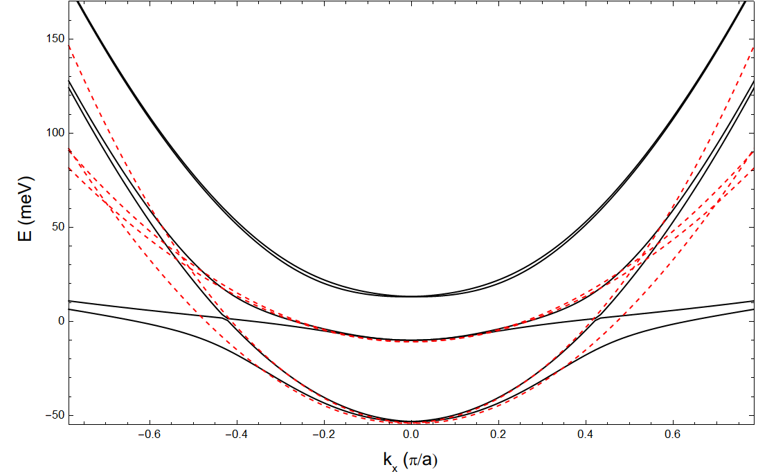
Figure 11: Comparison of the exact bands from Eq. (1) (black lines) with the bands of the effective Hamiltonians in Eqs. (16) and (17) (dashed lines).

APPENDIX 4: Additional pairings

In this Appendix , we discuss additional pairings which could be considered in the system.

In Eq. (19), an inter-site attraction between particles with opposite spins can be included, as well. Correspondingly, we considered also a triplet term related to a pairing between opposite spins. However, the self-consistent solution of the superconducting phase showed that this term is always zero in the range of $U$ and $V$ that we have considered in this paper. Actually, in the triplet pairing representation, this term would correspond to a vector $d_{z}({\bf k})$, which comes out to vanish. This is quite typical of two-dimensional superconductors with in-plane spin-orbit coupling frigeri2004 ; sato2010 , such as the one we consider here, while an out-of-plane spin-orbit coupling tends to favour a nonzero $d_{z}$. That $d_{z}({\bf k})=0$ can be already inferred from Eq. (17). Indeed, in frigeri2004 it has been shown that the superconducting transition temperature is maximized when the spin-triplet pairing vector $d({\bf k})$ (see Eq. (III.2)) is aligned with the polarization vector ${\bf g}({\bf k})$ parametrizing the spin-orbit coupling ($H_{\mathrm{SO}}({\bf k})={\bf g}({\bf k})\cdot{\bf\sigma}$). For $H_{0}^{(\mathrm{eff})}({\bf k})$ in Eq. (17) (neglecting the out-of-diagonal terms with power in the momenta higher than one, subleading around ${\bf k}=0$), we have

$$H_{0}^{(\mathrm{eff})}({\bf k})\approx\epsilon_{0}({\bf k})\,{\bf I}_{2\mathrm{x}2}+g_{1}({\bf k})\,\sigma_{x}+g_{2}({\bf k})\,\sigma_{y}\,,$$ (55)

with $g_{1}({\bf k})=0.8\,k_{x}$ and $g_{2}({\bf k})=-0.8\,k_{y}$, and $g_{3}({\bf k})=0$. Therefore it is expected that $d_{z}({\bf k})=0$.

Finally, it is worth commenting on the fact that, strictly speaking, we make the ansatz in Eq. (20) for the unrotated $\tau$-bands. However, the same ansatz can be adopted at least for the low-density regime of the $\eta_{-}$ and especially $\eta_{0}$ bands, the latter doublet being the regime where superconductivity is postulated gariglio2016 . Indeed, around ${\bf k}=0$, one gets (see Appendix 3 for details),

$$\eta_{0,\sigma}({\bf k})=\alpha_{(yz),\sigma}({\bf k})\,c_{(yz),\sigma}({\bf k})+\alpha_{(zx),\sigma}({\bf k})\,c_{(zx),\sigma}\,({\bf k})\,,$$ (56)

with $\big{(}\tau=(yz,zx)$):

$$|\alpha_{\tau,\sigma}({\bf k}\to 0)|=\frac{1}{\sqrt{2}}+O(k_{x}^{2})+O(k_{y}^{2})\,.$$ (57)

Therefore, since the same mapping is also diagonal in $\sigma$, it preserves, up to phases, the structure of the s-p pairing (at most linear in the momenta), at least around ${\bf k}=0$. This behaviour is even strengthened for the $\eta_{-}$ band, that results from the mixing around ${\bf k}=0$ of the $xy$ bands with the others: in fact, this mixing is suppressed by the energy gap $E_{t}$ in Eq. (5).

It is also worth stressing that we do not add a spin-singlet intersite contribution. Indeed, our analysis focuses on the regime of low filling, where the occupied electronic states are close to ${\bf k}=0$. In the small momentum limit, the spin-singlet intersite term would give rise to extended s-wave order parameter (ruled by a sum of cosines of the momentum) which would result in just a subleading additive contribution to the standard s-wave parameter induced by on-site attractive terms. Therefore, we neglected it, adding instead the leading nonzero contribution with equal spins (that is also more relevant once one turns on a magnetic field).

APPENDIX 5: Effects of inversion-symmetry breaking term

In Section IV of the main text, we have found a large regime for $U$ and $V$, where triplet and singlet pairings coexist in the first dome. Then we inferred that this mixing, allowed by $V$, stems from the parallel contributions of the spin-orbit term in Eq. (11) and of the inversion breaking one in Eq. (13). Indeed, at the effective level, they result together in the Rashba-like coupling of Eq. (17), known to induce a mixing of pairings with different parity rashba2001 . More in detail, in the same regime of energies, the contribution of Eq. (11) is dominant on that of Eq. (13) (vanishing at ${\bf k}=0$), a fact can be inferred also in the direct construction of Eq. (17).

It is important to investigate directly this effect of the spin-orbit term in Eq. (11) on the mixing of the pairings. For this purpose, we repeat the mean field procedure performed above, switching off the same term. In the resulting Fig. 12, again at fixed $U=350$ meV, $\frac{V}{2}=290$ meV, and $\mu=-9$ meV, it appears clear that Eq. (11) collaborates to enforce the triplet pairing, correspondingly lowering the singlet component. However, this effect does not look critical, changing the previously found behaviours only quantitatively. Therefore, the major role to the singlet-triplet mixing seems, in the analyzed regimes, to result from the $V$ term of the potential in Eq. (19), even for chemical potentials close to the Lifshitz point where the first dome starts. In turn, the $V$ term can be ascribed to the relatively low charge densities at the location of the dome. For these reasons, similar results are obtained at higher chemical potentials going from the first to the second dome. We ascribe the present result to the ability, described in Section III, of the mean-field approach to grasp the interplay between singlet and triplet components.

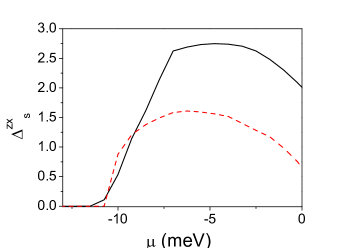
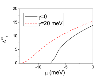
Figure 12: Singlet (Left panel) and triplet (right panel) pairing amplitudes (in meV) for the $\tau=zx$ bands, as a function of the chemical potential (in meV). The attractive couplings in Eq. (19) are set as $U=350$ meV and $\frac{V}{2}=290$ meV.

References

- (1) A. D. Caviglia, S. Gariglio, N. Reyren, D. Jaccard, T. Schneider, M. Gabay, S. Thiel, G. Hammerl, J. Mannhart, and J.-M. Triscone, Electric field control of the LaAlO3/SrTiO3 interface ground state, Nature 456, 624 (2008).
- (2) J. Biscaras, N. Bergeal, S. Hurand, C. Grossetete, A. Rastogi, R. C. Budhani, D. LeBoeuf, C. Proust, and J. Lesueur, Two-Dimensional superconducting phase in LAO/STO heterostructures induced by high-mobility carrier doping, Phys. Rev. Lett. 108, 247004 (2012).
- (3) L. P. Gorâkov, Back to Mechanisms of Superconductivity in Low-Doped Strontium Titanate, J. Supercond. Nov. Magn. 30, 845 (2017).
- (4) J. M. Edge, Y. Kedem, U. Aschauer, N. A. Spaldin, and A. V. Balatsky, Quantum Critical Origin of the Superconducting Dome in , Phys. Rev. Lett. 115, 247002 (2016).
- (5) J. Ruhman and P. A. Lee, Superconductivity at very low density: The case of strontium titanate, Phys. Rev. B 94, 224515 (2016).
- (6) S. Gariglio, M. Gabay, and J.-M. Triscone, Research Update: Conductivity and beyond at the LaAlO3/SrTiO3 interface APL Mater. 4, 060701 (2016).
- (7) D. Stornaiuolo, D. Massarotti, R. Di Capua, P. Lucignano, G. P. Pepe, M. Salluzzo, and F. Tafuri, Signatures of unconventional superconductivity in the LaAlO3/SrTiO3 two-dimensional system, Phys. Rev. B 95 (14), 140502 (2017).
- (8) E. Maniv, M. Ben Shalom, A. Ron, M. Mograbi, A. Palevski, M. Goldstein and Y. Dagan, Strong correlations elucidate the electronic structure and phase diagram of LaAlO3/SrTiO3 interface, Nat. Commun. 6, 8239 (2015).
- (9) A. M. R. V. L. Monteiro, M. Vivek, D. J. Groenendijk, P. Bruneel, I. Leermakers, U. Zeitler, M. Gabay, and A. D. Caviglia, Band inversion driven by electronic correlations at the (111) interface, Phys. Rev. B 99, 201102 (2019).
- (10) T. V. Trevisan, M. SchÃŒtt, and R. M. Fernandes, Unconventional Multiband Superconductivity in Bulk and Interfaces, Phys. Rev. Lett. 121, 127002 (2018).
- (11) P. Wójcik, M. P. Nowak, and M. Zegrodnik, Superconducting dome in doped 2D superconductors with broken inversion symmetry, Physica E 118, 113893 (2019).
- (12) M. Zegrodnik and P. Wójcik, Superconducting dome in LaAlO3/SrTiO3 interfaces as a direct consequence of the extended s-wave symmetry of the gap, Phys. Rev. B 102, 085420 (2020).
- (13) A. Jouan, S. Hurand, G. Singh, E. Lesne, A. Barthélémy, M.Bibes, C. Ulysse, G. Saiz, C. Feuillet-Palma, J. Lesueur, N. Bergeal, Origin of the dome-shaped superconducting phase diagram in SrTiO3-based interfaces, arXiv:2104.08220 .
- (14) G. Khalsa, B. Lee, and A. H. Mac Donald, Theory of electron-gas Rashba interactions, Phys. Rev. B 88, 041302 (2013).
- (15) M. Diez, A. M. R. V. L. Monteiro, G. Mattoni, E. Cobanera, T. Hyart, E. Mulazimoglu, N. Bovenzi, C. W. J. Beenakker, and A. D. Caviglia, Giant Negative Magnetoresistance Driven by Spin-Orbit Coupling at the Interface, Phys. Rev. Lett. 115, 016803 (2015).
- (16) Z. Zhong, A. Tóth, Anna and K. Held, Theory of spin-orbit coupling at LaAlO3/SrTiO3 interfaces and SrTiO3 surfaces, Phys. Rev. B 87, 161102 (2013).
- (17) M. Ben Shalom, M. Sachs, D. Rakhmilevitch, A. Palevski, and Y. Dagan, Tuning Spin-Orbit Coupling and Superconductivity at the Interface: A Magnetotransport Study, Phys. Rev. Lett. 104, 126802 (2019).
- (18) P. K. Rout, E. Maniv, and Y. Dagan, Link between the Superconducting Dome and Spin-Orbit Interaction in the (111) Interface, Phys. Rev. Lett. 119, 237002 (2017).
- (19) M. S. Scheurer and J. Schmalian, Topological superconductivity and unconventional pairing in oxide interfaces, Nat. Comm. 6, 6005 (2015).
- (20) N. Mohanta and A. Taraphder, Topological superconductivity and Majorana bound states at the LaAlO3/SrTiO3 interface, Europhys. Lett. 108, 60001 (2014).
- (21) F. Loder, A. P. Kampf, and T. Kopp, Route to Topological Superconductivity via Magnetic Field Rotation, Sci. Rep. 5, 15302 (2015).
- (22) Y. Fukaya. S. Tamura, K. Yada, Y. Tanaka, P. Gentile, and M. Cuoco, Interorbital topological superconductivity in spin-orbit coupled superconductors with inversion symmetry breaking, Phys. Rev. B 97, 174522 (2018).
- (23) J. Settino, F. Forte, C. A. Perroni, V. Cataudella, M. Cuoco, and R. Citro, Spin-orbital polarization of Majorana edge states in oxide nanowires, Phys. Rev. B 102, 224508 (2020).
- (24) A. Barthelemy, N. Bergeal, M. Bibes, A. Caviglia, R. Citro, M. Cuoco, A. Kalaboukhov, B. Kalisky, C. A. Perroni, J. Santamaria, Quasi-two-dimensional electron gas at the oxide interfaces for topological quantum physics, Europhys. Lett. 133, 1 (2021).
- (25) C. A. Perroni, V. Cataudella, M. Salluzzo, M. Cuoco, R. Citro, Evolution of topological superconductivity by orbital selective confinement in oxide nanowires, Phys. Rev. B 100, 094526 (2019).
- (26) A. Joshua, S. Pecker, J. Ruhman, E. Altman, and S. Ilani, A universal critical density underlying the physics of electrons at the LaAlO3/SrTiO3 interface, Nat Commun 3, 1129 (2012).
- (27) J. Biscaras, N. Bergeal, A. Kushwaha, T. Wolf, A. Rastogi, R. C. Budhani and J. Lesueur, Two-dimensional superconductivity at a Mott insulator/band insulator interface LaTiO3/SrTiO3, Nat. Commun. 1, 89 (2010).
- (28) N. Reyren, S. Thiel, A. D. Caviglia, L. F. Kourkoutis, G. Hammerl, C. Richter, C. W. Schneider, T. Kopp, A.-S. Ruetschi, D. Jaccard, M. Gabay, D. A. Muller, J.-M. Triscone, and J. Mannhart, Superconducting Interfaces Between Insulating Oxides, Science 317, 1196 (2007).
- (29) L. Taillefer, Scattering and pairing in Cuprate superconductors, Ann. Rev. Condens. Matter Phys. 1, 51 (2010).
- (30) B. Keimer, S. A. Kivelson, M. R. Norman, S. Uchida, and J. Zaanen, From quantum matter to high-temperature superconductivity in copper oxides, Nature 518, 179 (2015).
- (31) N. Boudjada, F. L. Buessen, and A. Paramekanti, Domes of in single-band and multiband superconductors with finite-range attractive interactions, Phys. Rev. B 102, 054504 (2020).
- (32) C. Yin, P. Seiler, L. M. K. Tang, I. Leermakers, N. Lebedev, U. Zeitler, and J. Aarts, Tuning Rashba spin-orbit coupling at interfaces by band filling, Phys. Rev. B 101, 245114 (2020).
- (33) G. Singh, A. Jouan, G. Herranz, M. Scigaj, F. Sanchez, L. Benfatto, S. Caprara, M. Grilli, G. Saiz, F. Couëdo, C. Feuillet-Palma, J. Lesueur, and N. Bergeal, Gap suppression at a Lifshitz transition in a multi-condensate superconductor, Nat. Mater. 18, 948â954 (2019).
- (34) N. Reyren, S. Gariglio, A. D. Caviglia, D. Jaccard, T. Schneider, and J.-M. Triscone, Anisotropy of the superconducting transport properties of the LaAlO3/SrTiO3 interface, Appl. Phys. Lett. 94, 112506 (2009).
- (35) L. P. Gor’kov and E. I. Rashba, Superconducting 2D System with Lifted Spin Degeneracy: Mixed Singlet-Triplet State, Phys. Rev. Lett. 87, 037004 (2001).
- (36) M. Alidoust, C. Shen, and I. Zutic, Cubic spin-orbit coupling and anomalous Josephson effect in planar junctions, Phys. Rev. B 103, 060503 (2021).
- (37) H. Tajima, Y. Yerin, A. Perali, and P. Pieri, Enhanced critical temperature, pairing fluctuation effects, and BCS-BEC crossover in a two-band Fermi gas, Phys. Rev. B 99, 180503(R) (2019).
- (38) P. Rosenberg, H. Shi, and S. Zhang, Ultracold Atoms in a Square Lattice with Spin-Orbit Coupling: Charge Order, Superfluidity, and Topological Signatures, Phys. Rev. Lett. 119, 265301 (2017).
- (39) A. G. Swartz et al, Polaronic behavior in a weak-coupling superconductor, Proc. Natl. Acad. Sci. 115, 1475 (2018).
- (40) S. Sumita and Y. Yanase, Superconductivity induced by fluctuations of momentum-based multipoles, Phys. Rev. Research 2, 033225 (2020).
- (41) Z. S. PopoviÄ, S. Satpathy, and R. M. Martin, Origin of the two-dimensional electron gas carrier density at the LAO on STO interface, Phys. Rev. Lett. 101, 256801 (2008).
- (42) P. Delugas, A. Filippetti, V. Fiorentini, D. I. Bilc, D. Fontaine, and P. Ghosez, Spontaneous 2-dimensional carrier confinement at the n-type STO/LAO interface, Phys. Rev. Lett. 106, 166807 (2011).
- (43) N. Scopigno, D. Bucheli, S. Caprara, J. Biscaras, N. Bergeal, J. Lesueur, and M. Grilli, Phase separation from electron confinement at oxide interfaces, Phys. Rev. Lett. 116, 026804 (2016).
- (44) M. Salluzzo, J. C. Cezar, N. B. Brookes, V. Bisogni, G. M. De Luca, C. Richter, S. Thiel, J. Mannhart, M. Huijben, A. Brinkman, G. Rijnders, and G. Ghiringhelli, Orbital reconstruction and the two-dimensional electron gas at the LAO/STO interface, Phys. Rev. Lett. 102, 166804 (2009).
- (45) D. Valentinis, S. Gariglio, A. Fête, J.-M. Triscone, C. Berthod, and D. van der Marel, Modulation of the superconducting critical temperature due to quantum confinement at the LAO/STO interface, Phys. Rev. B 96, 094518 (2017).
- (46) G. Singh, A. Jouan, L. Benfatto, F. Couëdo, P. Kumar, A. Dogra, R.C. Budhani, S. Caprara, M. Grilli, E. Lesne, A. Barthélémy, M. Bibes, C. Feuillet-Palma, J. Lesueur, and N. Bergeal, Competition between electron pairing and phase coherence in superconducting interfaces, Nat. Commun. 9, 407 (2018).
- (47) A. P. Schnyder, S. Ryu, A. Furusaki, A. W. W. Ludwig, Classification of Topological Insulators and Superconductors, AIP Conf. Proc. 1134, 10 (2009).
- (48) C. K. Chiu, J. C.Y. Teo, A. P. Schnyder, and S. Ryu, Classification of topological quantum matter with symmetries, Rev. Mod. Phys. 88, 035005 (2016).
- (49) B. A. Bernevig and T. L. Hughes, Topological Insulators and Topological Superconductors, (Princeton University Press, Princeton, NJ, 2013).
- (50) D. Stornaiuolo, C. Cantoni, G. M. De Luca, R. Di Capua, E. Di. Gennaro, G. Ghiringhelli, B. Jouault, D. Marré, D. Massarotti, F. Miletto Granozio, I. Pallecchi, C. Piamonteze, S. Rusponi, F. Tafuri, and M. Salluzzo, Tunable spin polarization and superconductivity in engineered oxide interfaces, Nat. Mater. 15, 278 (2016).
- (51) J. F. Annett, Superconductivity, Superfluids and Condensates, Oxford University Press, Oxford (2004).
- (52) A. P. Schnyder and P. M. R. Brydon, Topological surface states in nodal superconductors, J. Phys.: Cond. Matter 27 243201 (2015).
- (53) H. Nakamura, T. Koga, and T. Kimura, Experimental Evidence of Cubic Rashba Effect in an Inversion-Symmetric Oxide, Phys. Rev. Lett. 108, 206601 (2012).
- (54) D. van der Marel, J. L. M. van Mechelen, and I. I. Mazin, Common Fermi-liquid origin of resistivity and superconductivity in -type SrTiO3, Phys. Rev. B 84, 205111 (2011).
- (55) C. A. Perroni, G. De Filippis, and V. Cataudella, Ground-state features and spectral properties of large polaron liquids from low to high charge densities, Phys. Rev. B 103, 245130 (2021).
- (56) C. Pethick and H. Smith, Bose-Einstein Condensation in Dilute Gases, Cambridge University Press: Cambridge, UK, (2001).
- (57) M. M. Parish, F. M. Marchetti, A. Lamacraft, and B. D. Simons, Finite-temperature phase diagram of a polarized Fermi condensate, Nat. Phys. 3, 124-128 (2007).
- (58) D. E. Sheehy and L. Radzihovsky, BEC-BCS crossover, phase transitions and phase separation in polarized resonantly-paired superfluids, Ann. Phys. 322 1790 (2007).
- (59) M. Breitschaft, V. Tinkl, N. Pavlenko, S. Paetel, C. Richter, J. R. Kirtley, Y. C. Liao, G. Hammerl, V. Eyert, T. Kopp, and J. Mannhart, Two-dimensional electron liquid state at LaAlO3-SrTiO3 interfaces, Phys. Rev. B 81, 153414 (2010).
- (60) C. Cancellieri, A. S. Mishchenko, U. Aschauer, A. Filippetti, C. Faber, O. S. Barisic, V. A. Rogalev, T. Schmitt, N. Nagaosa, and V. N. Strocov, Polaronic metal state at the LaAlO3/SrTiO3 interface, Nat. Commun. 7, 10386 (2016).
- (61) K. Michaeli, A. C. Potter, and P. A. Lee, Superconducting and Ferromagnetic Phases in SrTiO3/LaAlO3 Oxide Interface Structures: Possibility of Finite Momentum Pairing, Phys. Rev. Lett. 108, 117003 (2012).
- (62) Y. Nakamura and Y. Yanase, Multi-Orbital Superconductivity in SrTiO3/LaAlO3 Interface and SrTiO3 Surface, J. Phys. Soc. Jpn. 82, 083705 (2013).
- (63) F. Loder, A. P. Kampf, and T. Kopp, Superconductivity with Rashba spin-orbit coupling and magnetic field, J. Phys: Condens. Matter 25, 362201 (2013).
- (64) N. Mohanta and A. Taraphder, Multiband theory of superconductivity at the LaAlO3/SrTiO3 interface, Phys. Rev. B 92, 174531 (2015).
- (65) X.-L. Qi, T. L. Hughes, S. Raghu, and S.-C. Zhang, Time-Reversal-Invariant Topological Superconductors and Superfluids in Two and Three Dimensions, Phys. Rev. Lett. 102, 187001 (2009).
- (66) M. Sato and Y. Ando, Topological superconductors: a review, Rep. Prog. Phys. 80 076501 (2017).
- (67) P. A. Frigeri, D. F. Agterberg, A. Koga, and M. Sigrist, Superconductivity without Inversion Symmetry: MnSi versus CePt3Si, Phys. Rev. Lett. 92, 097001 (2004).
- (68) K. V. Samokhin, in E. Bauer and M. Sigrist, Non-centrosymmetric Superconductors, (Springer-Verlag Berlin Heidelberg, 2012).
- (69) M. Sato, Nodal structure of superconductors with time-reversal invariance and Z2 topological number, Phys. Rev. B 73, 214502 (2006).
- (70) K. V. Samokhin, Symmetry and topology of two-dimensional noncentrosymmetric superconductors, Phys. Rev. B 92, 174517 (2015).
- (71) K. V. Samokhin and S. P. Mukherjee, Fermionic boundary modes in two-dimensional noncentrosymmetric superconductors, Phys. Rev. B 94, 104523.
- (72) N. Read and D. Green, Paired states of fermions in two dimensions with breaking of parity and time-reversal symmetries and the fractional quantum Hall effect, Phys. Rev. B 61, 10267 (2000).
- (73) Coleman S., The magnetic monopole fifty years later, in The Unity of the Fundamental Interactions, edited by Zichichi A. (Plenum, London) (1983).
- (74) S. Coleman, S. Coleman, Classical lumps and their quantum descendants, (1975), published in Aspects of symmetry (selected Erice lectures), Cambridge University Press (1985).
- (75) M. Nakahara, Geometry, Topology and Physics, 2nd edition (Institute of Physics, Bristol) (2003).
- (76) K. Yada, M. Sato, Y. Tanaka, and T, Yokoyama, Surface density of states and topological edge states in noncentrosymmetric superconductors, Phys. Rev. B 83, 064505 (2011).
- (77) More in detail, this Hamiltonian is recast at first in a off-diagonal block form, , via a transformation , such that . Then, defined , it holds n = , where the integral is performed on a close path around the node , where the p-wave pairing vanishes. Far from the points (in the space of the Hamiltonian parameters) where and vanish, , ( and are the charge-and time-conjugation unitary matrices, respectively), continuous in . Instead, where and vanish, is ill defined and can jump between 0 and 1. In our case, the phase is isomorphic to that encoded in Eq. (29), via Eq. (30). Moreover, the Bogoliubov Hamiltonian from the multiband model in Eq. (1), as well as and defined in the Appendix 1, can be exploited directly.
- (78) P. W. Anderson, Knight Shift in Superconductors, Phys. Rev. Lett. 3, 325 (1959).
- (79) G. Y. Cho, J. H. Bardarson, Y.-M. Lu, and J. E. Moore, Superconductivity of doped Weyl semimetals: Finite-momentum pairing and electronic analog of the 3He-A phase, Phys. Rev. B 86 214514 (2012).
- (80) J. H. Zhou, T. Qin, and J.-R. Shi, Intra-Valley Spin-Triplet Superconducting Pairing in Lightly Doped Graphene, Chin. Phys. Lett. 30 017401 (2013).
- (81) L. Lepori, A. Celi, A. Trombettoni, and M. Mannarelli, Synthesis of Majorana mass terms in low-energy quantum systems, New J. Phys. 20 063032 (2018).
- (82) G. Campagnano, P. Lucignano, D. Giuliano, and A. Tagliacozzo, Spin-orbit coupling and anomalous Josephson effect in nanowires, J. Phys.: Cond. Matt. 27 (20), 205301 (2015).
- (83) M. Minutillo, D. Giuliano, P. Lucignano, A. Tagliacozzo, and G. Campagnano, Anomalous Josephson effect in S/SO/F/S heterostructures, Phys. Rev. B 98 (14), 144510 (2018).
- (84) A. Maiellaro, F. Romeo, C. A. Perroni, V. Cataudella, and R. Citro, Unveiling signatures of topological phases in open Kitaev chains and ladders, Nanomat. 9 894 (2019).
- (85) S. Weinberg, The Quantum Theory of Fields, Quantum theory of fields, Vol. 2 (Cambridge University Press, 1996).
- (86) M. S. Dresselhaus and G. Dresselhaus, Group Theory: Application to the Physics of Condensed Matter, Springer-Verlag, Berlin Heidelberg (2008).
- (87) M. Sato, Y. Takahashi, and S. Fujimoto, Non-Abelian topological orders and Majorana fermions in spin-singlet superconductors, Phys. Rev. B 82, 134521 (2010).