RMQFMU: Bridging the Real World with Co-simulation
Technical Report

Abstract

In this paper we present an experience report for the RMQFMU, a plug and play tool, that enables feeding data to/from an FMI2-based co-simulation environment based on the AMQP protocol. Bridging the co-simulation to an external environment allows on one side to feed historical data to the co-simulation, serving different purposes, such as visualisation and/or data analysis. On the other side, such a tool facilitates the realisation of the digital twin concept by coupling co-simulation and hardware/robots close to real-time. In the paper we present limitations of the initial version of the RMQFMU with respect to the capability of bridging co-simulation with the real world. To provide the desired functionality of the tool, we present in a step-by-step fashion how these limitations, and subsequent limitations, are alleviated. We perform various experiments in order to give reason to the modifications carried out. Finally, we report on two case-studies where we have adopted the RMQFMU, and provide guidelines meant to aid practitioners in its use.

1 Introduction

Cyber-physical systems (CPSs) refer to systems that combine computational and physical processes, and play an important role in the development of intelligent systems. Using real world operation data could possibly facilitate smart decision-making [1]. Harnessing this potential is by no means trivial, with challenges including safety [2], reliability, and security [3], among others, that need to be tackled. Additionally, CPS development is a multi-disciplinary process, implying that different components will be modelled and validated by different tools used in the different involved disciplines. The evaluation of such complex systems can be performed through co-simulation [4]. The individual models are integrated into a multi-model, and the joint behaviour of the different components can thereafter be simulated in tandem. However, this is not sufficient, as CPSs together with their environment(s) are subject to continuous changes, and evolve through time, possibly diverging significantly from the initial co-simulated results [5]. Digital twins (DTs), defined as digital replicas of the physical components, also known as physical twins (PTs), can be used to follow the behaviour of the PTs and CPSs during operation, potentially through learning [6], by adapting the models, as well as performing different tasks such as monitoring or predictions. The DT and the aforementioned (or more) operations can be developed via the co-simulation of a modelled system that corresponds to the deployed CPS. In order to connect the deployed CPS to the DT, implementing data brokering between them becomes a necessity.

The work presented in this publication extends an existing Data-Broker called RabbitMQ FMU (RMQFMU) [7], to enable data brokering to and from an FMI2-enabled co-simulation. We present an experience report on applying RMQFMU to two actual cases undergoing development to become digital twin systems: an autonomous agriculture robot and a tabletop robot arm. As part of this experience report we present guidelines on how to configure the RMQFMU parameters by presenting various experiments that show their effects and relation to one another. Through the application of RMQFMU to the aforementioned cases and experiments several needs were discovered such as:

1. Data Platform - Get all available data instead of minimally-needed data to enable decision making - i.e. the possibility of skipping data to enable larger time steps.

2. Performance - RMQFMU shall be as fast as possible.

3. Data Delay - RMQFMU shall output the newest data if available.

To address need 1. and 2., the existing RMQFMU, henceforth referred to as RMQFMU_0, was realised with multi-threading instead of single-threading. This new multi-threaded version is referred to as RMQFMU_1. Experimentation related to detailing the configuration of RMQFMU_1 and its related effects led to the discovery of need 3. In order to mitigate 3. yet another version of RMQFMU was realised referred to as RMQFMU_2. More information is presented in section XX to XY.

The rest of this paper is organised as follows. The next section provides an overview of the FMI standard, the first version of the RMQFMU (RMQFMU₀), as well as some of the technologies employed in the realisation of the case-studies. In Section 3, we describe four scenarios with which we motivate the need for the RMQFMU. Afterwards, we informally derive the requirements for RMQFMU, based on the usage scenarios of interest. Section 4 presents RMQFMU_1,2, how it mitigates some inadequacies of RMQFMU₀, and how it compares to RMQFMU₀. Thereafter, in Section 5 the individual case-studies are described, and the results gained with RMQFMU_1,2 are presented. Moreover, a detailed comparison between RMQFMU₁ and RMQFMU₂ is made. Section 6 provides a set of guidelines meant to aid the use of RMQFMU₂. Concluding remarks and potential avenus for future work are presented in Section 7.

2 Background

In this Section we provide a brief summary on the relevant concepts for this work, such as co-simulation, FMI standard, master algorithms, and the tools we use for their realisation. Thereafter, we present the first released version of the RMQFMU (RMQFMU₀), which we have extended as presented in this paper.

2.1 Concepts and Tools

The realisation of CPSs and constituent systems is a cross-disciplinary process, where the different components are modelled using different formalisms and modelling tools [8]. In order to evaluate the behaviour of such systems as a whole, co-simulation techniques are used, which require the integration of the separate models into what are called multi-models [9]. For the latter to be possible, the tools used to produce the individual models need to adhere to some standard. One such standard is the Functional Mock-up Interface 2.0 for Co-simulation (FMI) [10] that defines the C-interfaces to be exposed by each model, as well as interaction constraints, packaging, and a static description format. An individual component that implements the FMI standard is called Functional Mock-up Unit (FMU). A co-simulation is executed by an orchestration engine that employs a given master algorithm. The master algorithm defines the progression of a co-simulation in terms of getting outputs via getXXX function calls, setting inputs via setXXX function calls, and stepping the individual FMUs in time via the doStep function calls. Common master algorithms are the Gauss-Seidel and Jacobi (the curious reader is referred to [8] for an overview of these algorithms and a survey on co-simulation). In this work, we use the open-source INTO-CPS tool-chain [11], for the design and execution of co-simulation multi-models, with Maestro [12] as orchestration engine employing an FMI-based Jacobi master algorithm.

2.2 Overview of the RMQFMU₀

RMQFMU₀ was implemented to enable getting external/historical data into the co-simulation environment, for either replaying such data in simulation, or for performing different kinds of analysis, e.g. checking its difference from expected data (the reader is referred to the Water-Tank Case-Study for an example). Essentially, RMQFMU₀ subscribes to messages with a specified routing key and outputs messages as regular FMU outputs at specific points in time based on the timestamp of the messages. At every call of the doStep function, the RMQFMU₀ attempts to consume a message from the server. A retrieved message is placed in an incoming queue, from which it is thereafter processed, according to the quality constraints (maxage and lookahead), described shortly. In case there is no data available, the RMQFMU₀ will wait for a configurable timeout before exiting. Note that, the doStep is tightly bound with the consuming operation, i.e. they are both contained within the main thread of execution. If on the other hand there is data, its validity with respect to time is checked. The maxage, main parameter of the RMQFMU₀, allows to configure the age of data within which the data is considered valid at a given time-step. Additionally, the lookahead parameter specifies how many messages will be processed at a step of RMQFMU and thereby at the given point in time. The behaviour of the RMQFMU₀ has been formally verified in previous work [7].

3 Motivation for the RMQFMU

The purpose of the RMQFMU is to serve as a bridge between an FMI-based co-simulation environment, and an external component, e.g. a simulator or hardware, that needs to be coupled with the co-simulation environment in order to achieve a predefined goal. We consider four scenarios in which such FMU is useful.

Data analysis and visualisation of system behaviour

In this case, the user of the RMQFMU is interested in feeding back to the co-simulation environment data recorded from the operation of the hardware, i.e. historical data, in order to perform some analysis on the data, potentially supporting the visualisation of said data, e.g. Water-Tank Case-study referred to in Section 2.

Co-simulation

In this scenario the user of the RMQFMU is interested in running a co-simulation of a given system. Some of the constituents of the system can behave as FMUs, while others cannot, e.g. a robot simulation in Gazebo, and therefore has to be connected to the co-simulation by other means.

Realisation of the Digital Shadow

In this scenario, digital models of the physical twin are contained within the co-simulation environment. The user is interested in getting the live data from the PT into the co-simulation environment in order to estimate the difference between actual and simulated data along with visualising the operation of the physical twin. This is similar to the first usage, the main difference being that here the digital shadow (DS) is operating with live data.

Realisation of the Digital Twin

In this scenario, the user is interested in enabling the communication link from the DS to the PT, thus fully realising the implementation of the DT concept. This means that there are components within the co-simulation environment that, based on the live data, are able to send live feedback to the PT.

This can be useful when we are monitoring the behaviour of the PT, e.g. consider a robot moving from point A to B. Assume an FMU that models the motion of the robot, and can be used to predict where the robot should be after some time given the starting point and velocity. As the live data of the robot’s position comes in, the divergence between the predicted and actual paths can be used to trigger an emergency stop to the robot . This setup can also be useful during the development of the robot, to ease and lower the cost of testing with Hardware in the Loop.

4 The RMQFMU

The design of the RMQFMU is based on a set of informally derived requirements, covering those functionalities needed for the adoption of the RMQFMU in the scenarios described in Section 3. These requirements are given as follows:

1. The RMQFMU is able to get the data published by an external system to the RabbitMQ server. This is relevant for all scenarios.

2. The RMQFMU is able to publish data to the RabbitMQ server, thus closing the communication link. This is relevant for the second and fourth scenario, i.e. for co-simulation and DT realisation.

3. The FMU steps as fast as possible. Indeed the role of the RMQFMU is that of a data broker, as such it is not part of the system being simulated, rather a facilitating entity. Therefore, the delays it causes should be minimal and impact the overall co-simulation environment as little as possible.

4. Provide quality constraints, e.g. with respect to age of data (maxage).

5. Provide performance constraints, e.g. number of messages processed per step (lookahead).

RMQFMU₀ already fulfils requirements 1 and 4. Requirement 5 is partially implemented in this version as well, in that while the lookahead determines how many messages to retrieve from the incoming queue at every time-step, there will not be more than one message at a time in this queue, given that a consume call is performed at the doStep call until a valid message is retrieved.

In order to tackle requirement 2, we enable the configuration of the inputs of the RMQFMU_1,2 as needed, i.e., a user can define as many inputs as desired, of one the following types: integer, double, boolean, and string. These inputs will be sent to the RabbitMQ server, on change; in other words, the values of the inputs will be forwarded if they have changed as compared to the previous step taken by the RMQFMU_1,2. This check is performed within the doStep, at every time-step.

In order to tackle requirement 3, we investigate the potential benefit of a threaded configuration of the RMQFMU_1,2. Indeed, the FMU allows for a build-time option to enable a multi-threaded implementation, with a separate thread to interface and consume data from the RabbitMQ server, parsing incoming data and placing it in the FMU incoming queue. The main doStep function of the FMU still executes in the main thread context of the calling simulation orchestration application, and it reads and processes data from the FMU incoming queue and produces outputs. If the multi-threaded option is disabled (default), the doStep function will consume data directly from the RabbitMQ server in the context of the calling main thread.

In general the potential performance benefits of the threaded implementation will depend on the amount of data being consumed, parsed, and provided in the internal incoming FMU queue when the doStep function is called. Hence, the benefits will depend largely on the co-simulation environment. If the co-simulation is fast, in vague terms if the delay between each call of the FMU doStep function is short compared to the rate of the incoming data, then the FMU will be mostly blocking for I/O. In this situation, the separate consumer thread may not provide much benefit as the doStep function will still need to wait/block for incoming data. On the other hand, if the co-simulation is slower compared to the rate of data, then the separate thread may be able to consume, parse, and provide data to the internal incoming FMU queue, in parallel to the main co-simulation thread running its orchestration engine and executing other potential FMUs or monitors. In addition, any performance benefits of a threaded implementation also depends largely on the execution platform having a multi-core processor and the OS/thread environment to be able to take advantage.

The threaded implementation allows for the full realisation of the lookahead functionality, thus tackling requirement 5. The consumer thread is continuously retrieving data – when available – and placing these messages in the incoming queue, from where said data is processed in chunks of lookahead size.

5 Experiments

The RMQFMU_1,2 has been evaluated with a series of experiments, across different combinations of parameters such as the maxage and lookahead, and in two different case-studies. The purpose of these setups is to provide an understanding on the performance of the RMQFMU_1,2, parameter tuning, as well as provide some insight into the effect of external factors. The first case-study presents a scenario based on data from a deployed industrial robot, thus adequately representing an industrial case. As a result, we perform the performance evaluation in this case-study. Additionally, we add mockup components to the co-simulation structure, to mimic a more realistic co-simulation with different components for different purposes, such as data analysis, prediction among others. Additionally, we consider the impact of external factors, such as the frequency of sending data to the RMQFMU_1,2. Whereas, the second case-study presents a setup with the Gazebo simulation of the Robotti agricultural robot [13], rather simple both in terms of the size of the messages being sent and the internal structure of the co-simulation. The parameters of interest are the lookahead, maxage, and the frequency with which we send data into the RMQFMU_1,2.

The experimentation is divided in two phases. In the first, we evaluate the impact of the multi-threaded implementation on the performance of the RMQFMU. Specifically, we compare RMQFMU₁ to RMQFMU₀, and argue for the suitability of adopting the multi-threaded configuration as the primary implementation for the RMQFMU. Additionally we consider the effects of the maxage and lookahead for RMQFMU₁. In the second phase, we evaluate the alterations to RMQFMU₁, i.e. RMQFMU₂, in order to tackle the side effects observed in phase 1, providing both performance and behaviour results.

5.1 Case-study 1: Universal robot 5e (UR)

This case study concerns an industrial robot called UR5e (Figure 1). The robot has a reach of 85 mm, payload of 5kg and 6 rotating joints. It is chosen because the UR5e is in production, thus represents a realistic component in a digital twin setting, and thereby a realistic amount of data. The data set is generated from a series of movements used for calibrating the digital twin to a related physical twin. Therefore, all joints are exercised. The test data from the UR robot used is present in csv format (35123 lines including the header) and consists of messages (excluding the header) with 107 float values (one being time) and 10 integer values. The messages have a sample rate (frequency $f_{data}$) of $2$ms and will be replayed/produced into the RabbitMQ broker with this rate. The test data contains a substantial number of time gaps, i.e. places where two consecutive messages in the input data are spaced with more than $2$ms. Data is replayed at a constant frequency of $2$ms and as such some messages are produced faster than their timestamps indicate. The effects of this will be discussed in the test results. Testsare also performed on a cleaned test data with a constant message spacing of $2$ms between all pairs of messages - i.e. no additional time gaps.

To investigate the behaviour of the FMU, we perform tests with different variations and relations between the simulation step size and the delay imposed by the simulation environment. We perform the tests with and without the threading option to investigate its effect, $t_{\mathit{on}}$ and $t_{\mathit{off}}$ respectively. We first consider simulation step duration and environment delays that simulates a setup where data is expected to be consumed as fast as its produced - i.e. every $2$ms and the overhead of the simulation delay is minimal. In this case we consider both the simulation step and the simulation delay to match the input data rate of $2$ms. Then we consider situations with larger simulation step duration and larger simulation delays - to mimic co-simulation environments with additional FMUs or monitors. The full list of test data used is provided in Table 6. In short, the results will provide an insight into how different parameters like frequency of input data, simulation step size, and simulation delay, and the relation of these parameters, influence the performance of the RMQFMU. Note, that for these tests we use a fixed lookahead of $1$ and a fixed maxage of $300$ms. The max age is chosen as such to cover for time gaps in the input data up to this range.

Figure 1: UR5e robot

Table 1: Tests for Case-study $1$ 

Sim step	Sim delay	Thread
Case 1	2ms	2ms	$t_{\mathit{off}}$
Case 2	2ms	2ms	$t_{\mathit{on}}$
Case 3∗	100ms	100ms	$t_{\mathit{off}}$
Case 4∗	100ms	100ms	$t_{\mathit{on}}$
Case 5	100ms	113ms	$t_{\mathit{on}}$
Case 6	100ms	120ms	$t_{\mathit{on}}$

5.2 Case-study 2: Gazebo Simulation of Robotti

The purpose of this case-study is to provide a basic example of a co-simulation coupled with the Gazebo simulation of the Robotti agricultural robot [13], through the RMQFMU, in order to gain insight into how the configurable parameters of the RMQFMU affect its behaviour. In this case the co-simulation environment consists of the RMQFMU and a monitor FMU. The data of interest in this scenario, i.e. the data sent through the RMQFMU consists of: the $x$ and $y$ positions of the robot, and the $x$ and $y$ position of the nearest obstacle. Additionally, a sequence number is attached to each message to keep track of the outputted messages during the processing of the results. The monitor takes as input such data, and computes the distance between the robot and obstacle for every time-step. In case such distance is below a predefined safety threshold, the monitor will issue an emergency stop to the Gazebo simulation of the robot.

Table 2: Overview of experiments for Case-study (CS) 2

CS 2	Parameters				CS 2	Parameters				CS 2	Parameters
	lA	mA	$t_{s}$	$f_{data}$		lA	mA	$t_{s}$	$f_{data}$		lA	mA	$t_{s}$	$f_{data}$
Case 1	1	0.2s	0.1	10Hz	Case 5	50	0.2s	0.1	500Hz	Case 9∗	2	0.4s	0.1	5Hz
Case 2	50	0.2s	0.1	10Hz	Case 6	200	2s	0.1	500Hz	Case 10∗	5	0.4s	0.1	5Hz
Case 3	1	2s	0.1	10Hz	Case 7	50	0.2s	0.1	500Hz	Case 11∗	2	2s	0.1	5Hz
Case 4∗	50	2s	0.1	10Hz	Case 8	200	2s	0.1	500Hz	Case 12∗	5	2s	0.1	5Hz

For this case-study we are interested in the following parameters (see Table 2), the maxage $mA$ of the messages, and the lookahead $lA$, and how they affect the behaviour of the RMQFMU, i.e. in terms of the sequence of messages outputted at every time-step. Note that for all the cases the threaded option is used ($t_{\mathit{on}}$). Parameters such as the size of the time-step $t_{s}$, the frequency of sending data $f_{data}$ to the co-simulation are fixed for cases $1-4$, such that they align. We argue such decision with the simplicity of the case-study, which could allow a user in reality to align these values. The time-step of the simulation is fixed to $0.1$s to provide adequate granularity. Whereas for cases $5-12$ we consider $f_{data}$ that doesn’t match the size of the simulation step, and observe the effects of the maxage and lookahead.

5.3 Phase 1 Results

5.3.1 Case-study 1

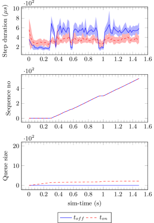
Figure 2: Case 1 and 2: step=2ms, delay=2ms, thread=$t_{\mathit{off}}$/$t_{\mathit{on}}$

First we consider the results of case 1 and case 2 from Table 6 (Figure 2). These tests are carried out with a simulation step matching the rate of incoming data at $2$ms and with a minimal simulation delay of also $2$ms. The running tests collect profiling information from the RMQFMU₁ consisting for each simulation step of: the step duration, which is the system execution time for the RMQFMU₁ doStep function, the sequence number output, which is the message sequence number output by the RMQFMU₁, and the queue size, which is the size of the internal incoming message queue in the RMQFMU₁. The tests are run $5$ times each to provide a minimal set of upper and lower bounds, and each test in this case runs for $1.5$sec simulation time.

A few things can be observed from the figure. First, it can be seen from the step duration graph (top, blue line), that the average step duration appears to be around $500$-$600$us with some drops to around $200$us in some periods. So, in general the step duration is lower than the $2$ms frequency of the input data, meaning that the RMQFMU₁ is capable of keeping up with the input data rate in this configuration.

The periods where the step duration drops to around $200$us are caused by two different reasons. The first period from simulation time $0$ to time $0.3$ is caused by the max age setting of $300$ms for this test. This max age means that the initial output value of the RMQFMU₁ is considered valid for the first $300$ms and hence no consumption of new RabbitMQ messages are needed for this period and as a result the step duration is low. From the middle graph (blue line) observe, that the unique message sequence number output by the RMQFMU₁ stays at the initial value for the first $300$ms. The second cause for the intermittent step duration drops as seen in the top graph (e.g. starting between time step $0.9$ and $1.0$) is due to time gaps in the input data. There are multiple occasions of consecutive input data messages being separated by much more than $2$ms in the test input data csv file. For the simulation steps happening during these gaps, no new input is provided and the max age causes the RMQFMU₁ to stay at its current output and hence the step duration is low. Finally, note from the bottom graph (blue line), that the RMQFMU₁ input queue size is constantly at $0$ after a simulation step has finished, since each simulation step consumes all (in this case $1$) messages from the RMQFMU₁ queue. However, the rabbitmq client library socket layer incoming queue may still increase.

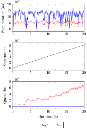
Figure 3: Cases 3 and 4: step=100ms, delay=100ms, thread=$t_{\mathit{off}}$/$t_{\mathit{on}}$

Now consider the same test but with the FMU configured to use the threaded setting. The results of this case are shown in Figure 2. Notice that the step duration (top, red dashed line) is now lower compared to the non-threaded case. From the graph, the step duration appears to be around $300-400$us. Compared to the non-threaded case with $500-600$us step durations, this is approximately $200-300$us lower. Which corresponds to the additional cost for consuming a single message from the RabbitMQ socket interface and parsing the JSON message format for the 117 message value references and placing the parsed message content in the internal FMU queue. In the threaded configuration, this message consumption executes in the separate consumer thread partly while the main thread delays for the configured $2$ms.

The same tests as above are also considered for cases 3 and 4, where the simulation step and the simulation delay is increased from $2$ms to $100$ms. This is done to mimic a co-simulation environment that imposes a step size of $100$ms and has a simulation delay also of $100$ms, caused e.g. by other FMUs or monitors. The results of these two tests are shown in Figure 3.

The results are equivalent to the results for cases 1 and 2. But as the simulation step size has increased to $100$ms, the number of messages to process in each step has now increased from $1$ to $50$ since the input frequency is still $2$ms. And since the simulation delay has also increased to $100$ms, it means that for the threaded configuration basically all $50$ messages will be available in the FMU queue when the step function is called. While for the non-threaded configuration, the step function itself needs to consume approximately $50$ messages of the socket interface inside a single step. As approximately $50$ messages need to be consumed in a single step, this accounts to an overhead of approximately $200\mu$s per message ($10$ms $/$ $50$ = $200\mu$s). And this corresponds to the observed difference in average step duration between the blue and red lines in Figure 3. So, for this configuration, the threaded configuration has a performance improvement of around $10$ms per step.

Also notice from Figure 3, that the queue size continually increases at the time points where the input data has time gaps as the FMU consumes no new inputs. The increase of queue size in the threaded configuration (red) is mostly an effect of gaps occurring in the input data. Large gaps in the input will cause the FMU to stay at its current output for a predefined maxage time period ideally covering the input gap. For this case-study, data is published with a fixed interval of $2$ms between consecutive messages, even though the message timestamps may be having larger gaps. I.e. this is an example of replaying historical data with a fixed message rate, as opposed to sending live data. Hence, for the gap periods, data will still be consumed by the separate FMU consumer thread and added to the internal queue. The FMU implementation must therefore include guards to respect internal queue size limitations. As discussed, the basic condition for a potential performance improvement using the threaded configuration will be present if the simulation step size is smaller than the simulation delay. If this condition is present, the number of messages to process in a simulation step may be already present in the FMU queue at the start of the step. And the total improvement gain is linear in the number of messages present in the queue. In our tests with a factor of around $200$us per message. The number of messages in the queue to be processed at each simulation step is determined by the relation between the input data frequency and the simulation step size.

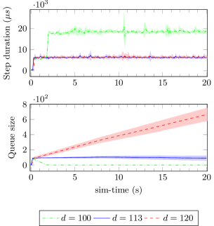
Figure 4: Case 5 and 6: step=100ms, delay=113 and 120ms, thread=on, cleaned input

The optimal relation between simulation step size and delay is very much system dependent and will vary. To observe the effects of increased simulation delays, we provide results for three tests with a fixed step size of $100$ms and three increasing delays of $100$ms, $113$ms, and $120$ms. Furtermore, as described earlier, the time gaps in the input data will reflect in the test results as time points where the FMU will not consume inputs and the output will be unchanged. And since the test environment still replays the delayed messages with a fixed interval (here of $2$ms), the input queue size will increase in these points. As a result, the FMU may have improved step duration caused by the fact of having time gaps in the input while still replaying it with a fixed interval. To remove the effect of this issue, these final tests are using a “cleaned” data set, meaning that there is a fixed timestamp interval of exactly $2$ms between all messages. I.e. the data has been ”cleaned” from gaps. The results are shown in Figures 4.

The test results with a simulation delay of $100$ms is shown in Figure 4 (green line). From this test it can be observed, that the $100$ms delay is actually too close to the step size to provide enough time for the input queue too constantly be filled with enough messages to process in the simulation step. The results show, that the input queue increases initially, but within the first $2$ seconds, the simulation has stepped fast enough for the FMU to gradually empty its queue. From that point onwards, the FMU will not have enough messages present in its queue to cover the entire simulation step. Hence, it needs to block for I/O to obtain new messages, and thus the step duration increases. Increasing the tested simulation delay to $113$ms provides just enough additional delay time for the input queue to have enough data for the tested time range of $20$sec (Figure 4 blue line). Notice that the step duration is constantly lower compared to the previous test. Finally, increasing the tested simulation delay to $120$ms provides no additional improvement in the step duration, but rather has the effect of having the FMU input queue increasing continually (Figure 4 dashed red line).

5.3.2 Case-study 2

Results for cases $1-4$ are displayed in Figure 5. It is possible to observe that for a low value of the maxage ($200$ms), there is no impact from changing the value of the lookahead. In contrast, for higher values of the maxage ($2$s), a higher value of the lookahead allows to jump to the latest messages valid for the time-step that we want to reach – those steps for which the current values are not valid with respect to the maxage, thus a new value is needed.

Whereas, a low value of the lookahead will result in older messages being outputted by the RMQFMU₁. The message that is outputted at a particular time-step depends on what is available in the queue at that particular time. We can observe in Figure 8, with a lookahead equal to $50$ and maxage fixed to $2000$ms, over 5 independent runs, that the number of skipped messages is not the exactly the same from run to run.. One factor that impacts the state of the queue is the speed of the execution of a simulation step. In Figure 8, one can observe the wall-clock time for two of the simulation runs. The first run is executed faster than real-time, at least until until time step $2.0$, whereas the second is executed slower than real-time. This depends on the underlying execution environment, as well as the load on said environment. As such, a specific lookahead will not necessarily output the same sequence numbers at each time step over different independent runs.

Results for cases $5-8$ can be observed in Figure 6, whereas for cases $9-12$ in Figure 7, consistent with what is observed in Figure 5. For a maxage equal to $400$ms, we can see that there is not much an effect of the value set for the lookahead. This is due to the fact that with lower maxage, the data becomes invalid sooner than for higher maxage, thus triggering the RMQFMU₁ to fetch newer data from the incoming queue. Nevertheless, for a maxage equal to $2$s, it is possible to note a difference for the two lookahead values, where for $la=5$, we can see a bigger jump in the sequences of data for specific time-steps, when a new value is needed. Additionally, sequence numbers remain fixed for a consecutive number of time-steps, whereas for $la=2$ more in-between value are outputted, as expected. Nevertheless, in the latter, there is more delay in the output values.

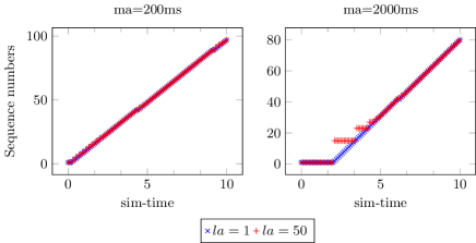
Figure 5: Messages outputted by the RMQFMU₁ at every step, with varying values of the maxage and the lookahead, for $f_{data}=100$ms.

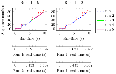
Figure 6: Messages outputted by the RMQFMU₁ at every step, with varying values of the maxage and the lookahead, for $f_{data}=2$ms.

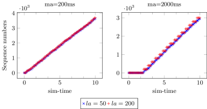
Figure 7: Messages outputted by the RMQFMU₁ at every step, with varying values of the maxage and the lookahead, for $f_{data}=200$ms.

The number of skipped messages is not the exactly the same from run to run, as observed in Figure 8, with a lookahead equal to $50$ and maxage fixed to $2000$ms, over 5 independent runs. One factor that impacts the state of the queue is the speed of the execution of a simulation step. In Figure 8, one can observe the wall-clock time for two of the simulation runs. The first run is executed faster than real-time, at least until until time step $2.0$, whereas the second is executed slower than real-time. This depends on the underlying execution environment, as well as the load on said environment. As such, a specific lookahead will not necessarily output the same sequence numbers at each time step over different independent runs. This effect is also visible in Figures 5 and 7, where for the last seconds, for both values of the lookahead, the sequence numbers that are outputted are similar. This means that, there were no newer messages in the queue at those particular times, as the simulation was running faster than real-time.

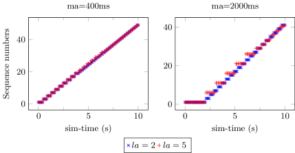
Figure 8: Messages outputted by the RMQFMU₁ at every step, over 5 runs, for maxage equal to $2000$ms and lookahead equal to $50$.

5.4 Phase 2 Results

As discussed in the previous results, the RMQFMU_0,1 has a rather conservative interpretation of the maxage parameter. The FMU will always stay at its current output, if the timestamp of the output is within maxage range from the current simulation step timestamp. This means that, the timestamp of the output plus the maxage is greater than or equal to the current simulation timestamp. However, this interpretation is rather strict, in the sense that it doesn’t take into account if newer data is present in the incoming FMU queue. Thus, we want to relax this condition such that the FMU will only stay at its current output, if the output is within the maxage and in addition there is no newer data available. In other words, the FMU should always move ahead to the latest input data valid within the current simulation step, and the maxage should only be considered when there is no new input.

We have implemented this change of maxage semantics in the RMQFMU₂ version of the FMU. The change itself had some side-effects impacting the performance of the FMU step function. Without going into details, the change means that the FMU now needs to consider if data is present before considering the maxage. However, situations may occur where data is present in the incoming queue, but it may have time-stamps in the future of the current simulation time. This can occur e.g. when replaying with a fixed interval historical data including gaps. If this situation occurs, the RMQFMU_0,1 versions of the FMU would move the future data from the incoming queue into an internal processing queue, that would gradually keep increasing in size and thereby impacting the step performance. To remedy this issue, RMQFMU₂ has an additional change to the internal queue structure. In the following paragraphs we present results of experiments with our two case-studies using RMQFMU₂.

5.4.1 Case-study 1

The effect of the RMQFMU₂ changes to the case-study 1 can be observed in Figure 9. The test configuration for this test is identical to Case 4 of Table 6. The results of this case with RMQFMU₁ are present in Figure 3. To demonstrate the effect of moving to the latest input data available, we have specified a lookahead size of $100$ in this test. This covers more messages than being produced on average within a simulation time step of $100$ms and a data frequency of $2$ms, which is approximately $100/2=50$ messages. So it basically means consuming as many messages as possible within a time step.

The middle graph in Figure 9 illustrates, that the seqno output increases within the initial maxage period of $300$ms. This, in contrast to the initial $300$ms period in the middle graph of Figure 3 where the output stays unchanged. It is possible to observe from Figure 9, top graph, that in contrast to Figure 3, the step duration now has decreased from around $6000$us to around $1000$us. This is due to the fact that we now use the larger (100 = move as close to step time as possible) lookahead size as opposed to the original size 1, additionally to the improvement in the internal queue implementation. Also, the larger lookahead size has the effect, that the queue size (right-hand side) stays low for a longer simulation time compared to earlier test results. But still the queue size starts increasing due to both data being produced more frequently than consumed and to gaps in the input data. Thus, as mentioned before, the FMU needs to guard any internal queue size limitations.

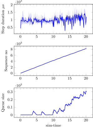
Figure 9: Step duration and sequence numbers outputted by RMQFMU₂ at every step, for $t_{\mathit{on}}$, and $f_{data}=2$ms.

5.4.2 Case-study 2

The new version of the RMQFMU₂ removes the delay in the outputted sequence numbers noticeable for large values of the maxage, e.g. $2000$ms (Figure 10, for Cases $1-4$), as compared to RMQFMU₁ (Figure 7). The utility of the maxage parameter becomes evident, once gaps are introduced in the data, in these experiments equal to $500$ms, Figure 11, left graph, and $1000$ms, right graph. It can be observed how when there is no input, the sequence value that is outputted is the last value that is valid from a time perspective. Naturally, for larger gaps, the sequence numbers outputted are more delayed, e.g. for $t=5$s, the RMQFMU₂ with $500$ms gaps is at number $10$, whereas for $1000$ms is at number $5$. Note, for the bottom graphs the lookahead is set to $10$ instead of $50$, however, that will not have an impact in the results, as with the given gaps, there cannot be more than $2$ and $1$ messages respectively (for $500$ms and $1000$ms delays) at a time in the queue.

Figure 10: Messages outputted by the RMQFMU₂ at every step, for $f_{data}=100$ms.

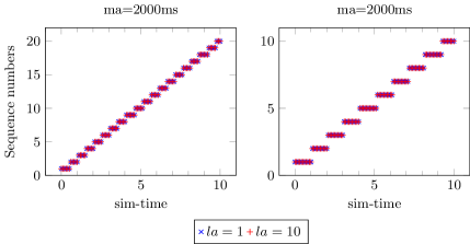
Figure 11: Messages outputted by the RMQFMU₂ at every step, for $f_{data}=100$ms with gaps of $500$ms (left), and $1000$ms (right).

In order to show the utility of the lookahead, we ran the experiments with simulation step-size equal to $100$ms, for values of maxage in {200ms, 2000ms}, with frequency of sending data equal to $500$Hz (Figure 12). For smaller values of the maxage, the delay of the RMQFMU₂ for lookahead equal to $1$, while consistently present, is rather low. However, for larger values of the maxage, the delay for low lookahead values is non-negligible. It is possible to observe that for the duration of the maxage the sequence numbers gradually increase by $1$, as expected for lookahead equal to $1$. However, after the initial maxage duration has passed, there is a jump in the sequence numbers, that continue to follow the results for lookahead equal to $50$, albeit with a more or less constant delay until the end. A similar effect was observed in Figure 7, with difference that in the current version, the RMQFMU₂ will check if there is a newer message which it can output. Such effect is due to the fact that after $2$s, older in-between values become invalid, and thus are not outputted, with RMQFMU₂ going back to the queue to pick up more recent messages.

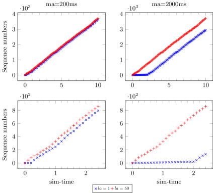
Figure 12: Messages outputted by the RMQFMU₂ at every step, for $f_{data}=2$ms, over $10$s (top graphs), zoomed in from $0-2$s (bottom graphs).

6 RMQFMU₂ Configuration Guidelines

The parameters of the RMQFMU₂ should be configured based on the use-case in order to result in desired behaviour. If possible, the simulation step-size should match the frequency of sending data $f_{data}$. However, depending on the time granularity needed by different FMUs, achieving such alignment might not be possible. The maxage value has to be big enough to make up for any time gap between data, but also low enough to ensure consistency in domain of use. E.g. for some applications, it might the case that data should not be older than $200$ms to ensure correct operation. The lookahead can be set to counter-balance the effect of the maxage, as it allows to jump to the latest data that is available in the queue (within the limits of the lookahead). Note however, larger values of the lookahead will result in bigger time jumps between the messages outputted. If more intermittent values are required, then a lower value should be adopted. The frequency of sending data influences the meaningful range of values for the lookahead, e.g. sending data every $2$ms, will result in $500$ messages per second. For a simulation step-size of $100$ms, a reasonable value of the lookahead would be circa $50$. Finally, the speed of the simulation also affects what is present in the queue at any time, as a result impacting RMQFMU₂ outputs.

7 Concluding Remarks

In this paper we have described an extended RMQFMU data-broker that enables coupling an FMI-based co-simulation environment to a non-FMI external component, via the AMQP protocol. The RMQFMU supports communication in both directions, and can be used in different contexts ranging from replaying historical data into a co-simulation, to enabling the realisation of the DT concept by connecting the DT to its physical counterpart. We evaluate this component in terms of its performance, i.e. the real-time duration of a simulation step. Our results show the benefit of the implementation of a threaded solution, that effectively decouples the doStep logic from the consumption from the rabbitMQ server. Moreover, we explore different values of its configurable parameters, such as the maxage and lookahead, and provide guidelines that can help practitioners in the usage of the RMQFMU.

There are four main directions for future work. First, we are interested in enabling the RMQFMU to take bigger step-sizes if necessary, given that there is future data to jump to. In some monitoring applications, where only the latest data-points are relevant, such jump could be of use to mitigation components that deal with out of synchronisation situations, where the DT gets behind in time with respect to the PT. Second, we plan to formally verify the presented version of the RMQFMU, thus extending previous work that tackled the initial version of the RMQFMU [7]. Third, we intend to profile the overhead of RMQFMU as data-broker compared to an FMU that directly queries a database, for example in the context of large amounts of data. Finally, we will enable the master-algorithm to learn the optimal step-sizes automatically and deal with recurring variation at run-time. This will devoid design-time decisions and adjust step-sizes during run-time as needed.

References

- [1] A. Banerjee, K. K. Venkatasubramanian, T. Mukherjee, and S. K. S. Gupta. Ensuring safety, security, and sustainability of mission-critical cyber–physical systems. Proc. of the IEEE, 100(1):283–299, 2012.
- [2] R. Baheti and H. Gill. Cyber-physical systems. The impact of control technology, 12(1):161–166, 2011.
- [3] PMB ECSEL. Multi annual strategic research and innovation agenda for ecsel joint undertaking, 2016.
- [4] C. Gomes, C. Thule, D. Broman, P.G. Larsen, and H. Vangheluwe. Co-simulation: a Survey. ACM Comput. Surv., 51(3):49:1–49:33, May 2018.
- [5] J Fitzgerald, P.G. Larsen, and K. Pierce. Multi-modelling and co-simulation in the engineering of cyber-physical systems: towards the digital twin. In From Soft. Eng. to formal methods and tools, and back, pages 40–55. Springer, 2019.
- [6] J. Fitzgerald, K. Pierce, and P.G. Larsen. Co-modelling and co-simulation in the engineering of systems of cyber-physical systems. In Proc. of the Int. Conf. on System of Systems Engineering (SoSE), 2011.
- [7] C. Thule, C. Gomes, and K. G. Lausdahl. Formally verified fmi enabled external data broker: Rabbitmq fmu. In Proc. of the 2020 Summer Simulation Conference, SummerSim ’20, San Diego, CA, USA, 2020. Society for Computer Simulation International.
- [8] C. Gomes, C. Thule, D. Broman, P.G. Larsen, and H. Vangheluwe. Co-simulation: a survey. ACM Computing Surveys (CSUR), 51(3):1–33, 2018.
- [9] P.G. Larsen, J. Fitzgerald, J. Woodcock, P. Fritzson, J. Brauer, C. Kleijn, T. Lecomte, M. Pfeil, O. Green, S. Basagiannis, and A. Sadovykh. Integrated tool chain for model-based design of cyber-physical systems: The into-cps project. In Proc. of the Int. Workshop on Modelling, Analysis, and Control of Complex CPS, pages 1–6, 2016.
- [10] Modelica Association. Functional Mock-up Interface for Model Exchange and Co-Simulation. https://www.fmi-standard.org/downloads, October 2019.
- [11] J. Fitzgerald, C. Gamble, P.G. Larsen, K. Pierce, and J. Woodcock. Cyber-Physical Systems design: Formal Foundations, Methods and Integrated Tool Chains. In Proc. of the FME Workshop on Formal Methods in Software Engineering, Florence, Italy, May 2015. ICSE 2015.
- [12] C. Thule, M. Palmieri, C. Gomes, K. Lausdahl, H.D. Macedo, N Battle, and P.G. Larsen. Towards reuse of synchronization algorithms in co-simulation frameworks. In Proc. of the Int. Conf. on Soft. Eng. and Formal Methods, pages 50–66. Springer, 2019.
- [13] F. Foldager, O. Balling, C. Gamble, P.G Larsen, M. Boel, and O. Green. Design space exploration in the development of agricultural robots. In AgEng Conference. Wageningen, The Netherlands, volume 54, 2018.