AdaptSky: A DRL Based Resource Allocation Framework in NOMA-UAV Networks

Abstract

Unmanned aerial vehicle ($\tt{UAV}$) has recently attracted a lot of attention as a candidate to meet the 6G ubiquitous connectivity demand and boost the resiliency of terrestrial networks. Thanks to the high spectral efficiency and low latency, non-orthogonal multiple access (NOMA) is a potential access technique for future communication networks. In this paper, we propose to use the $\tt{UAV}$ as a moving base station (BS) to serve multiple users using NOMA and jointly solve for the 3D-$\tt{UAV}$ placement and resource allocation problem. Since the corresponding optimization problem is non-convex, we rely on the recent advances in artificial intelligence (AI) and propose AdaptSky, a deep reinforcement learning (DRL)-based framework, to efficiently solve it. To the best of our knowledge, AdaptSky is the first framework that optimizes NOMA power allocation jointly with 3D-$\tt{UAV}$ placement using both sub-6GHz and millimeter wave mmWave spectrum. Furthermore, for the first time in NOMA-UAV networks, AdaptSky integrates the dueling network (DN) architecture to the DRL technique to improve its learning capabilities. Our findings show that AdaptSky does not only exhibit a fast-adapting learning and outperform the state-of-the-art baseline approach in data rate and fairness, but also it generalizes very well. The AdaptSky source code is accessible to use here: https://github.com/Fouzibenfaid/AdaptSky

I Introduction

Future communication networks are envisioned to provide heterogeneous wireless communication services with significant performance boost over 5G networks [1]. Unmanned aerial vehicles ($\tt{UAV}s$), artificial intelligence (AI), millimeter wave (mmWave), along with some emerging medium access techniques are very key technologies in meeting such a goal [2]. For instance, thanks to their flexible 3D mobility, ease of deployment, and location precision, $\tt{UAV}s$ can serve as aerial base stations (BSs), and hence, augment or replace terrestrial BSs in some extreme scenarios [3]. Hence, it has become an active topic for different working groups in standardization bodies such as 3GPP [4].

Rendering to its ability to simultaneously share spectrum resources among multiple users, non-orthogonal multiple access (NOMA) promises for massive-devices connectivity making it a candidate access technique for beyond 5G systems. Moreover, when used in mmWave spectrum, NOMA offers a significant data rate boost. Nevertheless, efficiently managing resources for mmWave or even sub-6GHz spectrum for NOMA-$\tt{UAV}$ networks with a heterogeneous number of users is a complex problem [5]. In this perspective, we propose a novel advanced deep reinforcement learning (DRL)-based framework that solves jointly for the $\tt{UAV}$ placement and NOMA resource allocation in the context of sub-6GHz as well as mmWave spectrum.

There are few works available about NOMA-$\tt{UAV}$ networks, some of which have focused on $\tt{UAV}$ placement and NOMA resources allocation [6, 7, 8, 9]. The issues, however, with these works that, for simplicity they $i)$ assume links between users and $\tt{UAV}s$ are dominated by line-of-sight (LoS), as it is the case with [8, 7, 6], $ii)$ restrict the number of users in the network to two, e.g. [9, 7], $iii)$ solve for $\tt{UAV}$ placement and NOMA power allocation disjointly, for example [6], and/or $iv)$ limit the $\tt{UAV}$ analysis to 2D placement, e.g. [6, 9, 7, 8]. There have been some attempts in handling the 3D-placement problem of $\tt{UAV}$ such as in [10, 11, 12]. Yet, these works disjointly optimize the altitude and the 2D-$\tt{UAV}s$ placement. Imposing restrictions in analyzing 3D networks, can lead to inefficient use of resources. Hence, some innovative techniques that can handle their sophisticated analysis are needed.

A remarkable success has been reported for AI from incorporating DRL into the field of gaming [13]. DRL, which is mainly a reinforcement learning (RL) technique combined with deep-neural-network (DNN), has the potential to handle high-dimensional inputs, learn patterns, and solve complex problems efficiently [13, 14]. It has recently witnessed a number of advances to improve DRL learning abilities, speed, and generalization. Even though some initial works consider DRL for 2D-$\tt{UAV}s$ placement in the presence of LoS links only, e.g. [15], which employs deep deterministic policy gradient (DDPG) DRL, the full potentials of DRL for 3D networks still need to be assessed. Integrating dueling network architectures with DRL has shown its merits in dramatically improving and generalizing learning in the Atari domain [16]. In the same regard, dueling DRL, compared to other DRL advances like double DRL, as discussed in the $\tt{UAV}$ sensing related application context [17], shows an improvement in the learning speed. Nevertheless, there are surprisingly very limited research investigations done about integrating dueling DRL and $\tt{UAV}$. We aim, in this paper, to solve the non-convex optimization problem of the 3D-network resources management using our proposed dueling DRL based framework.

In this paper, we aim to bring forth the most-recent advances in AI to efficiently solve the $\tt{UAV}$ placement and resources management while maximizing both users' data rate and fairness. Our main contributions are summarized as follows

1. We propose a unified model-free framework, AdaptSky, for 3D $\tt{UAV}$ placement and power allocation in a NOMA-based network. We integrate dueling network with DRL, for the first time in NOMA-UAV networks, and demonstrate the tremendous-gain resultant in learning model generalization, and hence, network performance.

2. We show that AdaptSky is robust for different channel gain models both for the sub-6GHz and mmWave spectrum.

3. We show that AdaptSky maximizes the spectral efficiency while maintaining high users' fairness. Simulation results shows that AdaptSky outperforms other optimization based mathematical framework approach.

II System model

Figure 1: System model.

II-A Network Model

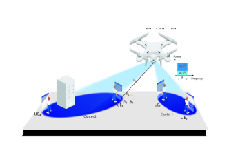
We consider a downlink cellular network with a $\tt{UAV}$ serving $\tt{N_{UE}}=2{N}$ ground users distributed randomly over an area $\mathcal{A}$ of $L\times L$ units and grouped into a number of clusters. To get the most out of NOMA, two users with distinct channel qualities get associated to a single cluster based on the strategy proposed in [5]. The $\tt{UAV}$ serves each cluster over an orthogonal resource with a total power $P_{T}$ distributed between the two corresponding users. The $\tt{UAV}$ is also assumed to be equipped with $\mathcal{N}_{\tt{UAV}}$ antennas while each user is equipped with $\mathcal{N}_{\tt{UE}}$ antennas, unless specified otherwise. Throughout the paper, user $i$ is denoted by ${\tt{UE}}_{i}$ where $i\in\{1,2,..,\tt{N_{UE}}\}$. Without loss of generality, we assume that users ${\tt{UE}}_{i}$ and ${\tt{UE}}_{i+1}$ for $i\in\{1,3,..,\tt{N_{UE}}-1\}$ are associated with the same cluster and $\tt{UE}_{i}$ has a stronger channel gain than ${\tt{UE}}_{i+1}$. The received power at the ${\tt{UE}}_{i}$ at a given time step $\tau$ can be expressed as

$$\hat{P}_{i,\tau} = P_{T}{g}_{i,\tau}^{\tt{MIMO}}(d_{i,\tau}){\alpha}_{i,\tau},$$ (1)

where ${g}^{\tt{MIMO}}_{i,\tau}(d_{i,\tau})$ is the channel gain between the $\tt{UAV}$ and ${\tt{UE}}_{i}$ separated, at time $\tau$, by a 3D distance $d_{i,\tau}$. Considering only a large scale fading, small scale fading is deferred for future works, and assuming a slight difference between antenna pairs, the channel gain can be approximated as ${g}^{\tt{MIMO}}_{i,\tau}(d_{i,\tau})=G{g}_{i,\tau}(d_{i,\tau})$, where $G=\mathcal{N}_{\tt{UAV}}\times\mathcal{N}_{\tt{UE}}$. ${g}_{i,\tau}(d_{i,\tau})$ is the channel gain between one UAV-${\tt{UE}}_{i}$ antenna pair. ${\alpha}_{i,\tau}$ is the power allocation coefficient that determines the amount of power, out of $P_{T}$, the $\tt{UAV}$ assigns to ${\tt{UE}}_{i}$ at the time step $\tau$.

II-B Signal-to-Interference-plus-Noise Ratio (SINR)

Following the NOMA protocol, the superposition coding (SC) is used at the $\tt{UAV}$ to transmit messages for users located in the same cluster. SC encodes different messages into a single signal while assigning them different power values. The successive interference cancellation (SIC) is used at the receiver side for signal detection. The received SINR at ${\tt{UE}}_{i}$ is expressed as

$$SINR_{i,\tau}=\frac{P_{T}\times{g}_{i,\tau}(d_{i,\tau})\times G\times\alpha_{i,\tau}}{P_{T}\times{g}_{i,\tau}(d_{i,\tau})\times G\times\beta_{i,\tau}+\sigma^{2}},$$ (2)

where $\beta_{i,\tau}=\alpha_{i-1,\tau}$ if $i$ is even and zero otherwise. $\sigma^{2}$ is the noise power. The first term in the denominator of equation (2) represents the interference from the user with the best channel condition to the other user. Based on the SIC technique, however, the interference at the user with the best channel condition gets canceled, which is the intuition behind the definition of $\beta_{i,\tau}$. For a bandwidth $W$, the data rate of ${\tt{UE}}_{i}$ at $\tau$ is given by

$$R_{i,\tau}=W\log_{2}(1+SINR_{i,\tau}).$$ (3)

II-C Channel Model

We consider to explore the performance of our system in both mmWave and sub-6GHz spectrum in the presence of the LoS and NLoS links. To accommodate for the various links and spectrum technologies, we modify the channel gain notation to be ${g^{k,sp}_{i,\tau}}(d_{i,\tau})$, where $k\in\{\tt{LoS},\tt{NLoS}\}$ and $sp\in\{\tt{mmWave},\tt{sub-6}\}$.

II-C1 MmWave Channel Model

Following the same model as in [18], at time step $\tau$, the $\tt{UAV}$-$\tt{UE}_{i}$ link is assumed to be in LoS with a probability $Pr^{\tt{LoS},\tt{mmWave}}_{i,\tau}(\theta_{i,\tau})$ given as

$$Pr^{\tt{LoS},\tt{mmWave}}_{i,\tau}(\theta_{i,\tau})=\frac{1}{1+C\exp[-Y(\theta_{i,\tau}\frac{180}{\pi}-C)]},$$ (4)

where $C$ and $Y$ are environment parameters, $\theta_{i,\tau}$ is the elevation angle between the $\tt{UAV}$ and $\tt{UE}_{i}$. Similarly, $\tt{UE}_{i}$ is assumed to be in NLoS using the complement property. The channel gain equation ${g}^{k,\tt{mmWave}}_{i,\tau}(d_{i,\tau})$ between the $\tt{UAV}$ located at a distance $d_{i,\tau}$ from $\tt{UE}_{i}$, according to [19] is expressed as

$${g}^{k,\tt{mmWave}}_{i,\tau}(d_{i,{\tau}})=C_{k}d_{i,\tau}^{-a_{k}},$$ (5)

where $a_{k}$ is the path loss exponent, and $C_{k}$ is the unit distance path loss.

II-C2 Sub-6GHz Channel Model

Similar to [20], $\tt{UE}_{i}$ is assumed to be in LoS with a probability given by

$$Pr^{\tt{LoS},\tt{sub-6}}_{i,\tau}(\theta_{i,\tau})=C.(\theta_{i,\tau}-\theta_{0})^{Y},$$ (6)

where $C$ and $Y$ are frequency and environment dependent parameters. $\theta_{0}$ is the minimum angle allowed by the model. Similarly, $\tt{UE}_{i}$ is assumed to be in NLoS using the complement property $Pr^{\tt{NLoS},\tt{sub-6}}_{i,\tau}(\theta_{i,\tau})=1-Pr^{\tt{LoS},\tt{sub-6}}_{i,\tau}(\theta_{i,\tau})$. The channel gain model for the $\tt{UE}_{i}$ is defined as

$${g}_{i,\tau}^{k,\tt{sub-6}}(d_{i,\tau})=\big{(}\frac{c}{4\pi f_{c}d_{i,\tau}}\big{)}^{2}10^{-0.1\eta_{k}},$$ (7)

where $f_{c}$ is the carrier frequency, and $(\frac{c}{4\pi f_{c}d_{i,\tau}}\big{)}^{2}$ represents the free space path loss. $\eta_{k}$, measured in dB, is the mean additional loss for transmission link [20].

II-D $\tt{UAV}$ Mobility Model

At time step $\tau$, the $\tt{UAV}$ is assumed to be placed at $(x_{\tt{UAV},\tau},y_{\tt{UAV},\tau},h_{\tt{UAV},\tau})$ and able to move to $(x_{\tt{UAV},\tau}+d_{x}\delta_{x},y_{\tt{UAV},\tau}+d_{y}\delta_{y},h_{\tt{UAV},\tau}+d_{h}\delta_{h})$, where $d_{x}$, $d_{y}$, and $d_{h}$ $\in\{1,-1\}$. $\delta_{x}$, $\delta_{y}$, and $\delta_{h}$ are the magnitude of change in the $x$ and $y$ axis, and height, respectively. $h_{\tt{UAV},\tau}\geq h_{0}$, by assumption. We assume that at $\tau=0$, the $\tt{UAV}$ is located at $(0,0,h_{\tt{UAV},0})$, where $h_{\tt{UAV},{0}}$ is the initial height. Without loss of generality, we assume the $\tt{UAV}$ can collect the channel state information (CSI) at the beginning of each time step [21].
The system model is shown in Fig. 1. For simplicity, $\tau$ is dropped for system parameters in the figure.

III 3D-$\tt{UAV}$ Placement and Power Allocation Formulation

We propose to optimize the $\tt{UAV}$ placement and power allocation that maximizes the total users' data rate and fairness. First, we define the sum users' data rate at time step $\tau$ as

$$R_{\tau}^{\textrm{tot}}=\sum_{i=1}^{\tt{N_{UE}}}W\log_{2}(1+SINR_{i,\tau}),$$ (8)

and, using the Jain's fairness index [22], the users' fairness as

$$J_{\tau}^{f}=\frac{(\sum_{i=1}^{\tt{N_{UE}}}R_{i,\tau})^{2}}{{\tt{N_{UE}}}\sum_{i=1}^{\tt{N_{UE}}}R_{i,\tau}^{{2}}}.$$ (9)

The optimization problem is formulated as the following

$$\max_{x_{\tt{UAV},\tau},y_{\tt{UAV},\tau},h_{\tt{UAV},\tau},\alpha_{i,\tau}}\omega_{r}\times R_{\tau}^{\textrm{tot}}+\omega_{f}\times J_{\tau}^{f},$$ (10a)

$$\alpha_{i,\tau}>0,\;\forall\;i\in\{1,..,\tt{N_{UE}}\},\;$$ (10b)

$${\alpha}_{i,\tau}+{\alpha}_{i+1,\tau}=1,\;\forall\;i\in\{1,3,..,\tt{N_{UE}}-1\},\;$$ (10c)

$$R_{i,\tau}\geq R_{min},\;\forall\;i\in\{1,..,\tt{N_{UE}}\},\;$$ (10d)

$$L/2\geq x_{\tt{UAV},\tau}\geq-L/2,\;$$ (10e)

$$L/2\geq y_{\tt{UAV},\tau}\geq-L/2,\;$$ (10f)

$$h_{\tt{UAV},\tau}\geq h_{0},\;$$ (10g)

$$\omega_{r}\geq 0,\;\omega_{f}\geq 0,$$ (10h)

where $R_{min}$ is a minimum required rate for each user.

Remark 1

To guarantee problem feasibility, the power allocation should satisfy: ${2^{({-R_{min}}/{W})}}>\alpha_{i,\tau}$, for $i\in\{1,3,..,\tt{N_{UE}}-1\}$, which follows from (10d).

The objective function in (10) is not convex, hence finding the optimal power allocation and $\tt{UAV}$ placement is challenging. Note that an optimal solution should strike a balance between two conflicting objectives: maximizing total users' data rate and users' fairness. These two objectives vary drastically based on users-to-$\tt{UAV}$ 3D distances, environment, and spectrum. Inspired by the recent advances and success of deep reinforcement learning, we propose an efficient framework that allows the $\tt{UAV}$ to learn how to maximize objectives, satisfy requirements, learn environment patterns, and adapt to related-unseen environments, and hence solve efficiently (10).

IV AdaptSky: Resource Allocation and $\tt{UAV}$ Placement Framework

IV-A Framework Preliminaries

Our reinforcement learning based framework is employed based on the Q learning method. We consider a sequential decision making setup, where the $\tt{UAV}$ interacts with the network environment which evolves as a Markov process over discrete time steps. At each time step, the $\tt{UAV}$ gets a representation of the environment state $s_{\tau}$, and takes an action $a_{\tau}$ drawn from a set of possible actions according to a certain policy $\pi$. The $\tt{UAV}$ moves to a new state $s_{\tau+1}$, and a reward $r_{\tau}$ is given as a consequence. The aim of the $\tt{UAV}$, starting from a time step $\tau$, is to determine the optimal policy, which is a series of actions, that maximizes the total discounted reward given by $\sum_{t=\tau}^{T-1}\gamma^{t-\tau}r_{\tau},$ where $\gamma\in[0,1]$ is a discount factor, and $T$ is the total number of time steps. The point of using a discounted reward is to make the $\tt{UAV}$ give more value to the nearest upcoming rewards. The Q-value of a state-action pair $(s_{\tau},a_{\tau})$ is the expected discounted reward obtained from taking action $a_{\tau}$ in state $s_{\tau}$. In the Q-learning method, a Q-table is used to store the Q-values for each state-action pair $Q\left(s_{\tau},a_{\tau}\right)$. The computational resources and time required for the iterative process of updating the table in a large state space makes conventional RL techniques inefficient for solving many optimization problems. DRL methods, nevertheless, like deep Q-learning (DQL) are emerging to handle environments represented by large and even continuous state space [13]. In DRL, DNNs are used to approximate the optimal Q-value for a state-action pair observed at $\tau$, $Q^{\ast}\left(s_{\tau},a_{\tau}\right)$, which is given by Bellman equation as

$$Q^{\ast}\left(s_{\tau},a_{\tau}\right) = \mathbb{E}\left[r_{\tau}+\gamma\max_{a_{\tau+1}}Q^{\ast}\left(s_{\tau+1},a_{\tau+1}\right)\right].$$ (11)

$Q^{\ast}\left(s_{\tau+1},a_{\tau+1}\right)$ is the optimal Q-value for the next state-action pair ($s_{\tau+1},a_{\tau+1}$). The policy DNN in DQL updates its parameters $\theta$ every time step $\tau$ with the objective of finding the optimal policy $\pi^{\ast}=\operatorname*{arg\,max}_{a}Q^{\ast}\left(s_{\tau},a_{\tau}\right)$. This is implemented by minimizing the loss $L(\theta)$, determined by comparing the outputs of the policy network $Q\left(s_{\tau},a_{\tau}\right)$ and target network, $r_{\tau}+\gamma Q^{\prime}\left(s_{\tau},a_{\tau}\right)$ and given by

$${L(\theta)=\mathbb{E}[\big{(}r_{\tau}+\gamma{\max Q^{\prime}(s_{\tau+1},a_{\tau+1})}-{Q(s_{\tau},a_{\tau})}\big{)}^{2}]}.$$ (12)

The target network, which improves stability of the DQL, has parameters $\theta^{\prime}$ which are cloned with the policy network parameter periodically. To improve the DRL stability even further, DRL randomly, at each time step, samples a mini-batch from an experience replay buffer that stores $s_{\tau},a_{\tau},s_{\tau+1}$ and $r_{\tau}$ to calculate the loss and updates the policy network parameters.

To enhance the learning process speed and generalization, we, furthermore, integrate the DN architecture with the DRL. In DN DRL, both target and policy networks have two output layers the value function, $V(s_{\tau})$, and advantage function, $A(s_{\tau},a_{\tau})$ defined as $A(s_{\tau},a_{\tau})=Q(s_{\tau},a_{\tau})-V(s_{\tau})$. The value function, defined as the expected value of the Q value, measures how good it is to be in a given state. The relative measure of the importance of an action at a particular state is indicated by the advantage function, however.

IV-B AdaptSky: DRL-based Framework

Based on the described advanced DRL method, we propose AdaptSky a framework that allows the $\tt{UAV}$ to efficiently position in a 3D plane while efficiently serving the different users. AdaptSky helps solve the optimization problem defined in (10). Nevertheless, setting up the right learning environment plays the crucial role in achieving so. Next, we formally describe how the states, actions, and rewards are designed.

1. States. A state $s_{\tau}$ describes the relative locations of the $\tt{UAV}$ to each user, user’s power coefficient, and $\tt{UAV}$-$\tt{UE}_{i}$ channel gain. $s_{\tau}$ is defined as $s_{\tau}=\big{[}s_{1,\tau}^{T},s_{2,\tau}^{T},...,s_{{\tt{N_{UE}}},\tau}^{T},h_{\tau}\big{]}^{T}$, where $s_{i,\tau}=\big{[}\Delta x_{\tt{UAV}-i,\tau},\Delta y_{\tt{UAV}-i,\tau},\alpha_{i,\tau},g_{i,\tau}(d_{i,\tau})\big{]}^{T}$, $\forall\;i\in\{1,..,\tt{N_{UE}}\}$. $\Delta x_{\tt{UAV}-i,\tau}$ and $\Delta y_{\tt{UAV}-i,\tau}$ are the step distance between the $\tt{UAV}$ and $\tt{UE}_{i}$ in the x-axis and y-axis respectively, and $h_{\tau}$ is the $\tt{UAV}$ current height. The initial sate, $s_{0}$, is set based on the predetermined initial $\tt{UAV}$ location $(0,0,h_{\tt{UAV},{0})}$ and power allocation coefficient $\alpha_{i,0}$ $\forall\;i\in\{1,..,\tt{N_{UE}}\}$. The cardinality of $s_{\tau}$ is $4\times\tt{N_{UE}}+1$.

2. Actions. An action $a_{\tau}$ is defined as $a_{\tau}=[d_{x}\delta_{x},d_{y}\delta_{y},d_{h}\delta_{h},\delta_{\alpha}^{T}]^{T}$ where $\delta_{\alpha}$ is defined as $[d_{1}\delta_{1},d_{3}\delta_{3},...,d_{\tt{N_{UE}}-1}\delta_{\tt{N_{UE}}-1}]^{T}$, $d_{i}\in\{1,-1\}$ and $\delta_{i}$ is the magnitude of change in the power allocation coefficient of $\tt{UE}_{i}$ $\forall i\in\{1,3,..,\tt{N_{UE}}-1\}$. $a_{\tau}$ determines the adjustments of the $\tt{UAV}$ 3D placement and the power allocated to all users. The action vector has a cardinality, denoted by $|A_{c}|$, of $3+\tt{N_{UE}}/2$.

3. Rewards. We define the reward at time step $\tau$ as

   $$\begin{split}r_{\tau}=w_{r}\times\frac{R_{\tau}^{\textrm{tot}}}{W}\times\prod_{i=1}^{\tt{N_{UE}}}\mathds{1}_{\big{(}\displaystyle R_{i,\tau}\geq R_{min}\big{)}}\\ +w_{f}\times J_{\tau}^{f}\times\mathds{1}_{\big{(}\displaystyle R_{min}=0\big{)}}+w_{g}\times g^{tot}_{\tau}\\ +w_{s}\times\sum_{i=1}^{\tt{N_{UE}}}\mathds{1}_{\big{(}\displaystyle R_{i,\tau}\geq R_{min}\big{)}}\\ +w_{u}\times\sum_{i=1}^{\tt{N_{UE}}}\frac{R_{i,\tau}}{W}\mathds{1}_{\big{(}\displaystyle R_{i,\tau}<R_{min}\big{)}},\end{split}$$ (13)

   where $g^{tot}_{\tau}$ defines the total users channel gain, $\mathds{1}_{(.)}$ is the indicator function. $w_{r}$, $w_{f}$, $w_{g}$, $w_{s}$, and $w_{u}$, with values greater than or equal to zero, are the weights corresponding to total rate, fairness, total channel gain, and satisfied and unsatisfied minimum rate requirements rewards respectively. The reward is designed carefully in terms of structure weights to make the $\tt{UAV}$ learn patterns to solve (10). The total rate reward term aims to increase the total sum rate after all users meet the minimum rate constraint to ensure fairness. The fairness reward term is only relevant when there is no fairness imposed through a minimum rate. It is intended to preclude the $\tt{UAV}$ from preferring some users over the rest. Without including such a reward, the $\tt{UAV}$ may end up favoring some users based on their channel conditions over others given the improvement they offer to the total rate specially in the presence of NLoS links. Even though, the impact of the channel gain is implicitly considered in the total rate reward, it makes the $\tt{UAV}$ learns channel conditions’ patterns and any related spatial variations. As a way to reinforce the $\tt{UAV}$ to satisfy the minimum rate requirement, at any time step $\tau$, a reward of $w_{s}$, which takes a relatively value, gets added to the total reward for every user achieves a rate that exceeds $R_{min}$. Users with a rate lower than $R_{min}$, however, get the unsatisfied minimum rate requirements reward, which aims mainly to encourage the $\tt{UAV}$ to keep improving users rate until the minimum rate requirements is satisfied.

Having described the different states, actions, and rewards, we describe AdaptSky and present it as in Algorithm 1. At the initialization, all DN DRL parameters are set. The policy network weights and biases ${\theta}$ are initialized randomly, and the target network parameters $\theta^{\prime}$ are cloned with ${\theta}$. Similarly, network environment is set and $\tt{UAV}$ location and power allocation coefficients are initialized. The decision process of AdaptSky is made over $E$ episodes with $T$ time steps each. To improve the learning experience at the beginning of each episode the $\tt{UAV}$ and power allocation are set back to their initial value. In our time sequential decision process, for a given state AdaptSky takes an action from the action space based on the $\epsilon$-greedy algorithm. To allow for exploring the action space, at any given time step, the $\tt{UAV}$ takes a random action with a probability $\epsilon$. Staring from $\epsilon_{s}$, $\epsilon$ gets decayed with a certain rate and converges to an ending value $\epsilon_{e}$. As a way to exploit the policy network decisions, however, with a complementary probability, the $\tt{UAV}$ takes the action that maximizes the Q-value which is constructed from the policy network outputs $V$ and $A$ values as $Q(s_{\tau},a_{\tau})\leftarrow V(s_{\tau})+A(s_{\tau},a_{\tau})-\frac{1}{|A_{c}|}\sum_{{a}_{\tau}}A(s_{\tau},a_{\tau})$. After executing $a_{\tau}$, the $\tt{UAV}$ observes the reward $r_{\tau}$ and the location and power coefficient to ensure that they are both feasible and modify the resultant state $s_{\tau+1}$ if needed. After that, states along with action and the resultant reward are stored in $\zeta$ that has a capacity $M$. Then, a mini-batch of $B$ is sampled from $\zeta$ and used to train the policy network such that the loss $L(\theta)$, found based on $Q$ and $Q^{\prime}$, is minimized using the gradient descent algorithm with a learning rate, $l_{r}$. $Q^{\prime}$ is constructed from target network output as $Q^{\prime}(s_{\tau+1},a_{\tau+1})\leftarrow V^{\prime}(s_{\tau+1})+A^{\prime}(s_{\tau+1},a_{\tau+1})-\frac{1}{|A_{c}|}\sum_{{a}_{\tau+1}}A^{\prime}(s_{\tau+1},a_{\tau+1})$. Accordingly, the policy notwork parameters $\theta$ are updated and similarly the target network parameters $\theta^{\prime}\leftarrow\theta$ after every $\delta$ time steps.

1 Initialization: Set up DN DRL parameters, and initialize policy network $Q$ with random parameters ${\theta}$ and target network parameters $\theta^{\prime}\leftarrow\theta$. Initialize network environment parameters including users and $\tt{UAV}$ locations, and allocated power

2 for episode ep= $0$:$E-1$ do

3       Receive state $s_{0}$

4       for $\tau$ = 0:$T-1$ do

5             Set $\epsilon\leftarrow\epsilon_{e}+(\epsilon_{s}-\epsilon_{e})\times e^{-\frac{(ep\times T+\tau)}{\chi}}$

6             Take $a_{\tau}$ based on $\epsilon$-greedy

7             Observe reward $r_{\tau}$ and next state $s_{\tau+1}$

8             If a $\tt{UAV}$ coordinate or a power coefficient is infeasible based on $a_{\tau}$, modify it with a unit magnitude of change and update $s_{\tau+1}$

9             Store experience ($s_{\tau},a_{\tau},r_{\tau},s_{\tau+1}$) in $\zeta$

10             Set $s_{\tau}\leftarrow s_{\tau+1}$

11             if experience memory size exceeds $B$ then

12                  Sample random mini-batch from $\zeta$

13                   Pass the mini-batch to the policy network

14                   Construct $Q(s_{\tau},a_{\tau})$ from $V$ & $A$

15                  

16                  Pass $s_{\tau+1}$ mini-batch to the target network

17                   Construct target Q-value $Q^{\prime}(s_{\tau+1},a_{\tau+1})$

18                   Calculate the loss $L(\theta)$

19                   Update $\theta$ such that $L(\theta)$ is minimized

20            

21      if ep is a multiple of $\delta$ then

22            Update weights and biases of the target network to the weights and biases of the policy network $\theta^{\prime}\leftarrow\theta$

23      

24

Algorithm 1 AdaptSky

V AdaptSky Performance Evaluation

V-A AdaptSky Implementation Details

AdaptSky networks consist of $2$ fully-connected layers of $128$ neurons each, and use ReLU as an activation function. $B$ and $M$ are taken to be $128$ and $15,000$, respectively. We employ $\epsilon_{s}=0.9$ and $\epsilon_{e}=0.1$. $\chi$, used in $\epsilon$ decaying rate, is set to $200$. Moreover, $l_{r}$, and $\gamma$ are chosen to be $0.001$ and $0.999$ respectively. We use Adam optimizer [23], which is adapted to noisy problems with sparse gradients, to update DNN parameters according to the value of the $l_{r}$. Target network parameters are updated every $10$ episodes. AdaptSky is trained for $E=1000$ episodes with $T=300$ time steps each. In addition to training, we deploy our AdaptSky trained model and test its decision performance over $1000$ time steps for network environment different than that set for the training.

V-B Network Settings

AdaptSky performance is tested for a $100\times 100$ $m^{2}$ area $\mathcal{A}$ with $\tt{N_{UE}}=4$ divided into $2$ clusters. Users $\tt{UE}_{1}$ and $\tt{UE}_{2}$ belongs to the same cluster based on their locations. The Cartesian coordinates of the users are set to $(x_{1},y_{1})=(4,15)$, $(x_{2},y_{2})=(-44,-49)$, $(x_{3},y_{3})=(-5,21)$ and $(x_{4},y_{4})=(47,49)$ in AdaptSky training scenarios and uniformly randomly distributed over $\mathcal{A}$ during the testing. The minimum $\tt{UAV}$ height $h_{0}$ is set to $10$ m. At the beginning of each episode, the initial height of the $\tt{UAV}$, $h_{\tt{UAV},0}$, is set to $50$ m and the power allocation coefficient $\alpha_{i,0}$ to $0.5$ $\forall i\in\{1,2,..,\tt{N_{UE}}\}$. $\delta_{x}$, $\delta_{y}$, and $\delta_{h}$ are all are set to be $1$ m. The magnitude of change in the power allocation is set for $0.01$ for all users. All channel model parameters for both mmWave and sub-6GHz are shown in Table I. The channel is modeled according to [19] which provides the New York city model.

TABLE I: Network parameters value.

Parameter	mmWave	sub-6GHz
Carrier frequency $f_{c}$	28GHz	2GHz
Transmit power $P_{T}$	$20$ dBm	$30$ dBm
Antenna configurations $\mathcal{N}_{\tt{UAV}}\times\mathcal{N}_{\tt{UE}}$	$8\times 8$	$1\times 1$
System bandwidth $W$	$2$ GHz	$50$ MHz
Thermal noise power $\sigma^{2}$	$-84$ dBm	$-88$ dBm
LOS probability parameter $C$	$9.6117$	$0.6$
LOS probability parameter $Y$	$0.1581$	$0.11$
Path loss intercept $C_{LoS}$	$10^{-6.4}$	-
Path loss intercept $C_{NLoS}$	$10^{-7.2}$	-
Mean additional LoS path loss $\eta_{LoS}$	-	$1$ dB
Mean additional NLoS path loss $\eta_{NLoS}$	-	$20$ dB
Path loss exponent $a_{LoS}$	$2$	-
Path loss exponent $a_{NLoS}$	$2.92$	-
Minimum elevation angle $\theta_{0}$	-	$15^{\circ}$

V-C Performance Analysis

In this subsection, we provide the performance of AdaptSky in managing the 3D NOMA-$\tt{UAV}$ network both during the training and testing cases. We compare our finding with the state-of-art technique in [6] which throughout the section will be referred to as SoA. The authors in [6], solve the NOMA power allocation and $\tt{UAV}$ placement problem using the conventional optimization framework. The $\tt{UAV}$ placement in [6] is restricted over a 2D plane which we set its height similar to AdaptSky initial height. They furthermore assume users to be only LoS. For simplicity, we only consider large scale fading and intend to study small scale fading and time-variability in our future work. For evaluation, we introduce the performance metrics ${R}_{e}^{\textrm{tot}}$ and $J_{e}^{f}$ which are defined as achieved average sum-rate and fairness index respectively. ${R}_{e}^{\textrm{tot}}$ ($J_{e}^{f}$) is determined by averaging the average rate (fairness index) per episode over the most recent $100$ episodes. ${R}_{e}^{\textrm{tot}}$ and $J_{e}^{f}$ both equal zero for all episodes $ep<100$.

V-C1 Performance of AdaptSky in the sub-6GHz spectrum

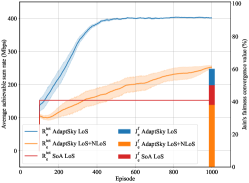
In Fig. 2, we depict ${R}_{e}^{\textrm{tot}}$ achieved by AdaptSkyfor both cases where users-$\tt{UAV}$ links are dominated by LoS and the case where the channel is generic. We also show the convergence value of the ${J}_{e}^{f}$ at $ep=E-1$. In LoS scenario, we set $w_{r}=1,w_{f}=0$, $w_{g}=10^{7}$, $w_{s}=0$ and $w_{u}=0$, with $R_{min}=0$, while in the generic scenario we set $w_{f}=5$ so that we prevent the $\tt{UAV}$ from favoring one user while ignoring the others (since it is the best way to achieve high sum rate with the existence of NLoS users). The rest of the weights are employed identical to the LoS case. The simulations have been conducted for 10 runs and the average and the confidence interval of 1 standard deviation of ${R}_{e}^{\textrm{tot}}$ has been calculated and plotted as shown in Fig. 2. AdaptSky tends to adapt the power allocation and $\tt{UAV}$ placement continuously such that ${R}_{e}^{\textrm{tot}}$ keeps improving until it convergences to a certain value. In our scenario, AdaptSky converges to $400$ Mbps, which is $163\%$ higher than that achieved by SoA. AdaptSky outperforms SoA despite the fact that AdaptSky is allocating resources in a more complex environment as the SoA can only place the $\tt{UAV}$ in a 2D plane and assumes LoS users. Moreover, Not only AdaptSky achieves a higher rate performance, but also maintains a $60\%$ fairness index which is more than $20\%$ higher than SoA. Although it is not reasonable to compare AdaptSky to SoA with the presence of NLoS users since SoA has only LoS users, AdaptSky achieves a better ${R}_{e}^{tot}$ and maintains a $40\%$ fairness level even though the NLoS results approximately in two orders of magnitude worse channel gain.

Figure 2: Average achievable rate versus episode and Jain's fairness index convergence value in sub-6GHz

V-C2 AdaptSky for mmWave-NOMA-$\tt{UAV}$ Networks

We below evaluate AdaptSky performance in terms of training and testing processes for different scenarios.
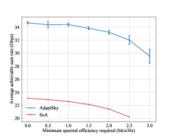
Training process. Assuming that channels are only LoS, throughout this analysis, we train AdaptSky to allocate resources by maximizing total average data rate while satisfying the minimum spectral efficiency specified by ${R}_{min}/W$. To satisfy the stated objective and constraint we set $w_{r}=10$, $w_{f}$ & $w_{g}$ to be zero, $w_{s}$ and $w_{u}$ to be $100$ and $10$ respectively. In Fig. 3, we plot ${R}_{e}^{\textrm{tot}}$ as a function of the minimum spectral efficiency along with the confidence interval of 6 runs. Observe that AdaptSky has a superior performance than SoA, thanks to its ability to relocate the $\tt{UAV}$ in the 3D plane while allocating power at the same time. In addition, AdaptSky managed to serve users while providing them with a minimum of $3$ bit/s/Hz while SoA could only handle up to $2.5$ bit/s/Hz given the same network resources and hence has a higher resources management efficiency.

Figure 3: Average achievable sum rate as a function of minimum spectral efficiency required in mmWave.

Testing process. In this scenario, we examine effectiveness, robustness and generalization ability of AdaptSky with respect to both SoA and conventional DRL method. We train AdaptSky  while setting $R_{min}$ to $0$, $w_{r}$ to be $10$, and all other weights to zero. We generated $100$ different users location realizations drawn from a uniform distribution and determined ${R}_{e}^{\textrm{tot}}$ based on actions taken, based on the trained policy network model, over a $1000$ consecutive time steps. In Fig. 4, we draw the average total sum rate percentage of AdaptSky compared with SoA and DRL. AdaptSky outperformed the DRL $67\%$ of locations with average of $39.11\%$ and up to $275.4\%$ improvement. This significant performance improvement of AdaptSky over DRL comes as a result of its higher generalization ability. Similarly, AdaptSky outperformed SoA over $91\%$ of locations with up to $90.25\%$ improvement and median of $30.25\%$.

Figure 4: AdaptSky achievable sum rate performance as a percentage of other techniques for different users location.

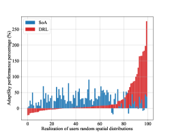
These results confirm that disjointing the power allocation and the $\tt{UAV}$ placement and restricting the $\tt{UAV}$ to 2D location lead to inefficient use of resources. Hence, these simulation results demonstrate the significant advantage of our proposed framework over the state-of-the-art, by unleashing the power of AI for solving the power allocation and the 3D-$\tt{UAV}$ placement jointly.

VI Conclusion

In this paper, we proposed AdaptSky, a novel AI-based framework built based on DRL with DN architectures. AdaptSky optimizes a $\tt{UAV}$ 3D location while allocating resources effectively in NOMA-$\tt{UAV}$ networks, simultaneously, for a generic-realistic channel gain for both sub-6GHz as well as mmWave technologies. Simulation results showed that AdaptSky yields significant performance gains over conventional approaches in terms of average achievable sum rate and fairness. Moreover, AdaptSky shows significant improvement in generalization over the DRL method.

References

- [1] Shuping Dang, Osama Amin, Basem Shihada, and Mohamed-Slim Alouini. What should 6G be? Nature Electronics, 3(1):20–29, 2020.
- [2] Khaled B Letaief, Wei Chen, Yuanming Shi, Jun Zhang, and Ying-Jun Angela Zhang. The roadmap to 6G: AI empowered wireless networks. IEEE Communications Magazine, 57(8):84–90, 2019.
- [3] Mostafa Zaman Chowdhury, Md Shahjalal, Shakil Ahmed, and Yeong Min Jang. 6G wireless communication systems: Applications, requirements, technologies, challenges, and research directions. IEEE Open Journal of the Communications Society, 1:957–975, 2020.
- [4] Xingqin Lin, Vijaya Yajnanarayana, Siva D Muruganathan, Shiwei Gao, Henrik Asplund, Helka-Liina Maattanen, Mattias Bergstrom, Sebastian Euler, and Y-P Eric Wang. The sky is not the limit: LTE for unmanned aerial vehicles. IEEE Communications Magazine, 56(4):204–210, 2018.
- [5] Yuanwei Liu, Zhijin Qin, Yunlong Cai, Yue Gao, Geoffrey Ye Li, and Arumugam Nallanathan. UAV communications based on non-orthogonal multiple access. IEEE Wireless Communications, 26(1):52–57, 2019.
- [6] Xiaonan Liu, Jingjing Wang, Nan Zhao, Yunfei Chen, Shun Zhang, Zhiguo Ding, and F Richard Yu. Placement and power allocation for NOMA-UAV networks. IEEE Wireless Communications Letters, 8(3):965–968, 2019.
- [7] Pankaj K Sharma and Dong In Kim. UAV-enabled downlink wireless system with non-orthogonal multiple access. In 2017 IEEE Globecom Workshops (GC Wkshps), pages 1–6. IEEE, 2017.
- [8] Fangyu Cui, Yunlong Cai, Zhijin Qin, Minjian Zhao, and Geoffrey Ye Li. Joint trajectory design and power allocation for UAV-enabled non-orthogonal multiple access systems. In 2018 IEEE Global Communications Conference (GLOBECOM), pages 1–6. IEEE, 2018.
- [9] Mehdi Monemi, Hina Tabassum, and Ramein Zahedi. On the performance of non-orthogonal multiple access (NOMA): Terrestrial vs. aerial networks. In 2020 IEEE Eighth International Conference on Communications and Networking (ComNet), pages 1–8, 2020.
- [10] Hajar El Hammouti, Mustapha Benjillali, Basem Shihada, and Mohamed-Slim Alouini. Learn-as-you-fly: A distributed algorithm for joint 3d placement and user association in multi-UAVs networks. IEEE Trans. on Wireless Communications, 18(12):5831–5844, 2019.
- [11] Mohamed Alzenad, Amr El-Keyi, Faraj Lagum, and Halim Yanikomeroglu. 3-d placement of an unmanned aerial vehicle base station (UAV-bs) for energy-efficient maximal coverage. IEEE Wireless Communications Letters, 6(4):434–437, 2017.
- [12] R Irem Bor-Yaliniz, Amr El-Keyi, and Halim Yanikomeroglu. Efficient 3-d placement of an aerial base station in next generation cellular networks. In 2016 IEEE international conference on communications (ICC), pages 1–5. IEEE, 2016.
- [13] Volodymyr Mnih, Koray Kavukcuoglu, David Silver, Alex Graves, Ioannis Antonoglou, Daan Wierstra, and Martin Riedmiller. Playing atari with deep reinforcement learning. arXiv preprint:1312.5602, 2013.
- [14] Volodymyr Mnih, Koray Kavukcuoglu, David Silver, Andrei A Rusu, Joel Veness, Marc G Bellemare, Alex Graves, Martin Riedmiller, Andreas K Fidjeland, Georg Ostrovski, et al. Human-level control through deep reinforcement learning. nature, 518(7540):529–533, 2015.
- [15] Chi Harold Liu, Zheyu Chen, Jian Tang, Jie Xu, and Chengzhe Piao. Energy-efficient UAV control for effective and fair communication coverage: A deep reinforcement learning approach. IEEE Journal on Selected Areas in Communications, 36(9):2059–2070, 2018.
- [16] Ziyu Wang, Tom Schaul, Matteo Hessel, Hado Hasselt, Marc Lanctot, and Nando Freitas. Dueling network architectures for deep reinforcement learning. In International conference on machine learning, pages 1995–2003. PMLR, 2016.
- [17] Kjell Kersandt, Guillem Muñoz, and Cristina Barrado. Self-training by reinforcement learning for full-autonomous drones of the future. In 2018 IEEE/AIAA 37th Digital Avionics Systems Conference (DASC), pages 1–10. IEEE, 2018.
- [18] Akram Al-Hourani, Sithamparanathan Kandeepan, and Simon Lardner. Optimal lap altitude for maximum coverage. IEEE Wireless Communications Letters, 3(6):569–572, 2014.
- [19] Mustafa Riza Akdeniz, Yuanpeng Liu, Mathew K Samimi, Shu Sun, Sundeep Rangan, Theodore S Rappaport, and Elza Erkip. Millimeter wave channel modeling and cellular capacity evaluation. IEEE journal on selected areas in communications, 32(6):1164–1179, 2014.
- [20] Akram Al-Hourani, Sithamparanathan Kandeepan, and Abbas Jamalipour. Modeling air-to-ground path loss for low altitude platforms in urban environments. In 2014 IEEE global communications conference, pages 2898–2904. IEEE, 2014.
- [21] Mohamed M El-Sayed, Ahmed S Ibrahim, and Mohamed M Khairy. Power allocation strategies for non-orthogonal multiple access. In 2016 International Conference on Selected Topics in Mobile & Wireless Networking (MoWNeT), pages 1–6. IEEE, 2016.
- [22] Rajendra K Jain, Dah-Ming W Chiu, William R Hawe, et al. A quantitative measure of fairness and discrimination. Eastern Research Laboratory, Digital Equipment Corporation, Hudson, MA, 1984.
- [23] Zijun Zhang. Improved adam optimizer for deep neural networks. In 2018 IEEE/ACM 26th International Symposium on Quality of Service (IWQoS), pages 1–2. IEEE, 2018.