Steady States of Holographic Interfaces
 

Abstract

We find stationary thin-brane geometries that are dual to far-from-equilibrium steady states of two-dimensional holographic interfaces. The flow of heat at the boundary agrees with the result of CFT and the known energy-transport coefficients of the thin-brane model. We argue that by entangling outgoing excitations the interface produces coarse-grained entropy at a maximal rate, and point out similarities and differences with double-sided black funnels. The non-compact, non-Killing and far-from-equilibrium event horizon of our solutions coincides with the local (apparent) horizon on the colder side, but lies behind it on the hotter side of the interface. We also show that the thermal conductivity of a pair of interfaces jumps at the Hawking-Page phase transition from a regime described by classical scatterers to a quantum regime in which heat flows unobstructed.

Laboratoire de Physique de l’École Normale Supérieure,
CNRS, PSL Research University and Sorbonne Universités
24 rue Lhomond, 75005 Paris, France

1 Introduction

AdS/CFT or holographic duality [1, 2, 3] reduces the study of certain strongly-coupled quantum systems to (semi)classical equations in gravity. The duality has been mainly tested and exploited at, or near thermal equilibrium, where a hydrodynamic description applies. For far-from-equilibrium processes our understanding is poorer. Indeed, although semiclassical gravity seems more tractable, highly-distorted horizons raise a host of unsolved technical and conceptual issues. To make progress, simple analytic models can be valuable. We will study one such model here.

A simple class of real-time processes are the non-equilibrium steady states (NESS) characterised only by persistent currents. These are particularly simple in critical (1+1) dimensional ballistic systems thanks to the power of conformal symmetry, see [5] for a review. On the gravity side the basic equilibrium states are the Banados-Teitelboim-Zanelli (BTZ) black strings [6, 7]. We deform the system by introducing a thin, but strongly back-reacting, domain wall anchored at a conformal defect or interface on the boundary. Our goal is to compute its stationary states.

Some properties of this thin-brane holographic model which will be useful later have been derived recently in refs.[10, 11, 12]. We rederive in particular the energy-transmission coefficients obtained from a scattering calculation in [10]. We also revisit the Hawking-Page, or deconfinement transition for a theory contained between a pair of interfaces [11, 12], and show that at the critical temperature the thermal conductivity undergoes a classical-to-quantum phase transition.

One phenomenon not discussed in these earlier works is the production of entropy. This is due to scattering at the interface, which entangles the outgoing excitations thereby mixing the reflected and transmitted fluids. A counter-intuitive feature of the thin-brane model is that the interfaces are perfect scramblers – the quantum fluids exit, as we will argue, thermalised. Whether this feature survives in top-down solutions with microscopic CFT duals is a question left for future work.

This scrambling behaviour is reminiscent of flowing black funnels [14, 15, 16, 17, 18], where a non-dynamical black hole acts as a source or sink of heat in the CFT. There are however important differences between the two setups. The non-back-reacting 1+1 dimensional black hole is a spacetime boundary that can absorb or emit arbitrary amounts of energy and entropy. Conformal interfaces, on the other hand, conserve energy and have a finite-dimensional Hilbert space. So even though one could mimic their energy and entropy flows by a two-sided boundary black hole whose (disconnected) horizon consists of two points with appropriately tuned temperatures, the rational, if any, behind such tuning is unclear.

The non-Killing event horizon of our solution is distorted far beyond the hydrodynamic regime. It lies behind the apparent horizon which is the union of the BTZ horizons on the two sides of the brane. At the point where the brane enters the event horizon this latter has discontinuous generators. Note that the event horizon is non-compact, thus evading theorems that exclude stationary non-Killing black holes [20, 21, 22]. The apparent horizon is also not compact, both far from the brane and at the brane-entry point. This prevents a clash with theorems [23] which show that event horizons always lie outside apparent (trapped-surface) ones.

The plan of the paper is as follows: In section 2 we review some well-known facts about the BTZ black string and its holographic interpretation (savvy readers can skim rapidly through this section). The black string is a rotating black hole with unwrapped angle variable and spin $J$ equal to twice the flow of heat in the dual CFT. For non-zero $J$ there is an ergoregion that plays a crucial role in our analysis.

In section 3 we explain, following ref. [24], why the flow of heat across a 2d conformal interface is proportional to the energy-transmission coefficient(s) of the interface. These transport coefficients are universal, independent of the nature of incident excitations [25]. By contrast, the coarse-grained entropy of the outgoing fluids depends a priori on details of the interface scattering matrix. If however the fluids are thermalised, as in our holographic model, their energy determines their (microcanonical) entropy.

Sections 4 to 7 contain the main results of our paper. In section 4 and in appendix A we solve the equations for a thin stationary brane between two arbitrary BTZ backgrounds. This generalizes the results of refs. [11, 12] to non-vanishing BTZ spin $J$. In section 5 we show that the brane penetrates the ergoregion if and only if the heat flow on the boundary agrees with the prediction from CFT and with the transmission coefficients computed by a scattering calculation in ref.[10]. We also show that once inside the ergoregion the brane cannot exit towards the AdS boundary, but crosses both outer BTZ horizons, hitting eventually either a Cauchy horizon or the singularity in one of the two regions.

Such a brane is dual to an isolated interface, and its non-Killing horizon is computed in section 6. We show that it coincides with the (local) BTZ horizon on the colder side of the interface, and lies behind but approaches it asymptotically on the hotter side. This is the evidence for perfect scrambling mentioned above. In section 7 we consider the system of an interface pair which is known to have an equilibrium Hawking-Page transition [11, 12]. We show that thermal conductivity jumps discontinuously at the transition point, from a classical regime of stochastic scattering to a deeply quantum regime in which heat flows unobstructed.

Section 8 contains closing remarks. In order to not interrupt the flow of the paper we have relegated the proof of some inequalities in appendix B, and background material on flowing black funnels in appendix C .

2 The boosted AdS₃ black string

The boosted black-string metric of three-dimensional gravity with negative cosmological constant reads

$$ds^{2}=\frac{\ell^{2}dr^{2}}{({r^{2}}-M\ell^{2}+{J^{2}\ell^{2}/4r^{2}})}-({r^{2}}-M\ell^{2})dt^{2}+r^{2}dx^{2}-J\ell\,dxdt\ ,$$ (2.1)

where $x\in\mathbb{R}$ is non-compact. If $x$ were an angle variable, (2.1) would be the metric of the rotating BTZ black hole [6, 7] with $M$ and $J$ its mass and spin  and $\ell$ the radius of AdS₃.

The metric (2.1) has an outer and an inner horizon located at

$$r_{\pm}^{2}={\frac{1}{2}}{M\ell^{2}}\pm{\frac{1}{2}}\sqrt{M^{2}\ell^{4}-J^{2}\ell^{2}}\,\,\ .$$ (2.2)

To avoid a naked singularity at $r=0$, one must require that $r_{+}$ be real which implies $M\ell\geq|J|$. In terms of $r_{\pm}$ the metric reads

$$\begin{split}&ds^{2}={\ell^{2}dr^{2}\over h(r)}-h(r)\,dt^{2}+(r\,dx-{J\ell\over 2r}\,dt)^{2}\ ,\\[4.30554pt] &\hskip-56.9055pt{\rm with}\qquad h(r)={1\over r^{2}}(r^{2}-r_{+}^{2})(r^{2}-r_{-}^{2})\qquad{\rm and}\qquad|J|={2r_{+}r_{-}\over\ell}\ .\end{split}$$ (2.3)

Besides $r_{\pm}$, another special radius is $r_{\rm ergo}=\sqrt{M}\,\ell\geq r_{+}$. It delimits the ergoregion inside which no observer (powered by any engine) can stay at a fixed position $x$.

Many properties of the metric (2.3) are familiar from the Kerr black hole. See [26] for a nice review. The outer horizon is a Killing horizon, while the inner one is a Cauchy horizon. Frame dragging forces ingoing matter to cross the outer horizon at infinity along the string, $x\sim J\ell\,t/2r_{+}^{2}\,\to\,\infty$. One can define ingoing Eddington-Finkelstein (EF) coordinates,

$$dv=dt+{\ell dr\over h(r)}\qquad{\rm and}\qquad dy=dx+{J\ell^{2}dr\over 2r^{2}h(r)}\ ,$$ (2.4)

in which the metric

$$ds^{2}\,=\,-h(r)\,dv^{\,2}+2\ell\,dv\,dr+r^{2}\big{(}dy-{J\ell\over 2r^{2}}\,dv\big{)}^{2}\$$ (2.5)

is non-singular at the (future) horizon. Outgoing coordinates can be defined similarly by changing $(x,t)\to(-x,-t)$ in (2.4).

2.1 Dual CFT₂ State

In the context of AdS/CFT, (2.1) describes a non-equilibrium steady state (NESS) of the CFT. This has been discussed in many places, see e.g. [27, 28, 29, 30, 31]. It can be seen explicitly from the general asymptotically-AdS solution of the vacuum Einstein equations, whose Fefferman-Graham expansion in three dimensions terminates [32]

$$ds^{2}={\ell^{2}dz^{2}\over z^{2}}+{1\over z^{2}}\Bigl{(}dx^{+}+\ell z^{2}\langle T_{--}\rangle dx^{-}\Bigr{)}\Bigl{(}dx^{-}+\ell z^{2}\langle T_{++}\rangle dx^{+}\Bigr{)}\ .$$ (2.6)

Here $\langle T_{\pm\pm}\rangle$ are the expectation values of the left-moving and right-moving energy densities in the dual CFT₂ state. The two metrics, (2.1) and (2.6), can be related by the change of coordinates

$$x^{\pm}=x\pm t\ ,\qquad r^{2}={1\over z^{2}}\Bigl{(}1+\ell z^{2}\langle T_{--}\rangle\Bigr{)}\Bigl{(}1+\ell z^{2}\langle T_{++}\rangle\Bigr{)}\ ,$$ (2.7)

and the identification

$$\text{\footnotesize${1\over 2}$}\,J\,=\,\langle T_{--}\rangle-\langle T_{++}\rangle\qquad{\rm and}\qquad\text{\footnotesize${1\over 2}$}\,{M\ell}\,=\,\langle T_{--}\rangle+\langle T_{++}\rangle\ .$$ (2.8)

It follows that the dual state has constant fluxes of energy in both directions, with a net flow $\langle T^{\,tx}\rangle=J/2$. To abide with the standard notation for heat flow we will sometimes write $J/2=dQ/dt$.

Generic NESS are characterised by operators other than $T_{\alpha\beta}$, for instance by persistent U(1) currents. To describe them one must switch on non-trivial matter fields, and the above simple analysis must be modified. The vacuum solutions (2.1) describe, nevertheless, a universal class of NESS that exist in all holographic conformal theories.

There are many ways of preparing these universal NESS. One can couple the endpoints $x\sim\pm\infty$ to heat baths so that left- and right-moving excitations thermalise at different temperatures $\Theta_{\pm}$ . An alternative protocol (which avoids the complications of reservoirs and leads) is the partitioning protocol. Here one prepares two semi-infinite systems at temperatures $\Theta_{\pm}$, and joins them at some initial time $t=0$. The steady state will then form inside a linearly-expanding interval in the middle [5]. In both cases, after transients have died out one expects

$$\langle T_{\pm\pm}\rangle={\pi c\over 12}\,\Theta_{\pm}^{2}={\pi^{2}\ell}\,\Theta_{\pm}^{2}\ \quad\Longrightarrow\quad\langle T^{\,tx}\rangle={\pi c\over 12}\,(\Theta_{-}^{2}-\Theta_{+}^{2})\ ,$$ (2.9)

where $c=12\pi\ell$ is the central charge of the CFT. Equation (2.9) for the flow of heat is a (generalized) Stefan-Boltzmann law with Stefan-Boltzmann constant $\pi c/12$. Comparing (2.9) to (2.8) relates the temperatures $\Theta_{\pm}$ to the parameters $M$ and $J$ of the black string. To implement the partitioning protocol on the gravity side it is sufficient to multiply the constant $\langle T_{\pm\pm}\rangle$ in eq. (2.6) by step functions $\theta(\pm\,x^{\pm})$.

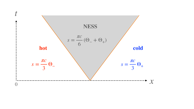
Figure 1: When two identical semi-infinite quantum wires at temperatures $\Theta_{\pm}$ are joined at $t=0$, a NESS forms inside an interval that expands at constant speed in both directions [5]. The entropy density $s(t,x)$ is shown in the three regions of the protocol. The energy density profile is identical, except for the replacement $\Theta_{\pm}\to{1\over 2}\Theta_{\pm}^{2}$.

It is interesting to also consider the flow of entropy. This is illustrated in figure 1 which shows the entropy density $s\equiv\langle s^{t}\rangle$ in the three spacetime regions of the partitioning protocol. Inside the NESS region there is constant flow of entropy from the hotter towards the colder side

$$\langle s_{\pm}\rangle=\pm{\pi c\over 6}\,\Theta_{\pm}\ .$$ (2.10)

The passage of the right-moving shock wave increases the local entropy at a rate $\pi c(\Theta_{-}-\Theta_{+})/6$, while the left-moving wave reduces it at an equal rate. Total entropy is therefore conserved, not surprisingly since there are no interactions in this simple conformal 2D fluid.

One can compute the entropy on the gravity side with the help of the Hubeny-Rangamani-Ryu-Takayanagi formula [33, 34]. For a boundary region of size $\Delta x$ the entanglement entropy reads [34]

$$S_{q\,\rm ent}={c\over 6}\log\big{[}{\beta_{+}\beta_{-}\over\pi^{2}\epsilon^{2}}\sinh({\pi\Delta x\over\beta_{+}})\sinh({\pi\Delta x\over\beta_{-}})\big{]}\ ,$$ (2.11)

where $\beta_{\pm}=\Theta_{\pm}^{-1}$ and $\epsilon$ is a short-distance cutoff. From this one computes the coarse-grained entropy density in the steady state

$$s_{\rm NESS}=\ \lim_{\Delta x\to\infty}{S_{q\,\rm ent}\over\Delta x}={\pi c\over 6}\,(\Theta_{-}+\Theta_{+})=2\pi\,r_{+}\ .$$ (2.12)

The last equality, obtained with the help of eqs. (2.9), (2.8) and (2.2), recasts $s_{\rm NESS}$ as the Bekenstein-Hawking entropy of the boosted black string (recall that our units are $8\pi G=\hbar=1$). This agreement was one of the earliest tests [35] of the AdS/CFT correspondence

3 NESS of interfaces

Although formally out-of-equilibrium, the state of the previous section is a rather trivial example of a NESS. It can be obtained from the thermal state by a Lorentz boost, and is therefore a Gibbs state with chemical potential for the (conserved) momentum in the $x$ direction.

More interesting steady states can be found when left- and right-moving excitations interact, for instance at impurities [24, 36, 37] or when the CFT lives in a non-trivial background metric [14, 15, 17]. Such interactions lead to long-range entanglement and decoherence, giving NESS that are not just thermal states in disguise.

The case of a conformal defect, in particular, has been analyzed in ref.[24]. As explained in this reference the heat current is still given by eq. (2.9) but the Stefan-Boltzmann constant is multiplied by ${\mathcal{T}}$, the energy-transmission coefficient of the defect. The relevant setup is shown in figure 2. The fluids entering the NESS region from opposite directions are thermal at different temperatures $\Theta_{1}\not=\Theta_{2}$. The difference, compared to the discussion of the previous section, is that the two half wires ($j=1,2$) need not be identical, or (even when they are) their junction is a scattering impurity.

3.1 Energy currents

If ${\mathcal{R}}_{j}$ and ${\mathcal{T}}_{j}$ are the reflection and transmission coefficients for energy incident on the interface from the $j$th side, then the energy currents in the NESS read 

$$\begin{split}&\langle T_{--}^{(1)}\rangle={\pi c_{1}\over 12}\,\Theta_{1}^{2}\ ,\qquad\langle T_{++}^{(1)}\rangle={\mathcal{R}}_{1}{\pi c_{1}\over 12}\,\Theta_{1}^{2}+{\mathcal{T}}_{2}{\pi c_{2}\over 12}\,\Theta_{2}^{2}\ ,\\[4.30554pt] &\langle T_{--}^{(2)}\rangle={\pi c_{2}\over 12}\,\Theta_{2}^{2}\ ,\qquad\langle T_{++}^{(2)}\rangle={\mathcal{T}}_{1}{\pi c_{1}\over 12}\,\Theta_{1}^{2}+{\mathcal{R}}_{2}{\pi c_{2}\over 12}\,\Theta_{2}^{2}\ .\end{split}$$ (3.1)

We have used here the key fact that the energy-transport coefficients across a conformal interface in 2d are universal, i.e independent of the nature of the incident excitations. The proof [25] assumes that the Virasoro symmetry is not extended by extra spin-2 generators, which is true in our holographic model. We have also used that the incoming and outgoing excitations do not interact away from the interface.

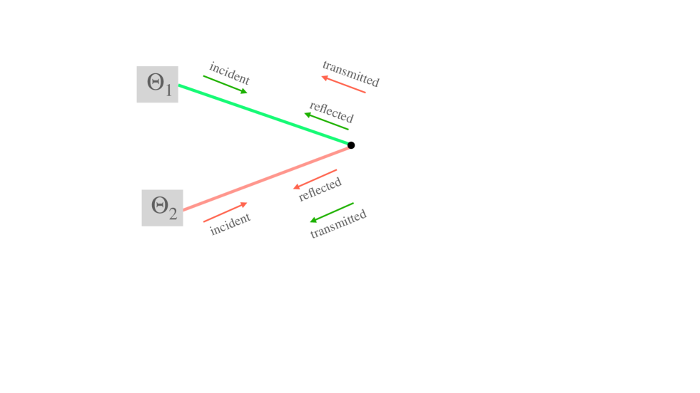
Figure 2: The energy fluxes given in (3.1). The two half wires are coloured red and green, and space is folded at the interface (black dot). The incoming excitations are thermal while the state of the outgoing ones, consisting of both reflected and transmitted fluids, depends on the nature of the junction as discussed in the main text.

Conservation of energy and the detailed-balance condition (which ensures that when $\Theta_{1}=\Theta_{2}$ the heat flow stops) imply the following relations among the reflection and transmission coefficients:

$${\mathcal{R}}_{j}+{\mathcal{T}}_{j}=1\qquad{\rm and}\qquad c_{1}{\mathcal{T}}_{1}=c_{2}{\mathcal{T}}_{2}\ \,.$$ (3.2)

Hence, only one of the four transport coefficients is independent. Without loss of generality we assume that $c_{2}\geq c_{1}$, i.e. that CFT₂ is the theory with more degrees of freedom. The average-null-energy condition requires $0\leq{\mathcal{R}}_{j},{\mathcal{T}}_{j}\leq 1$, so from (3.2) we conclude

$$0\leq{\mathcal{T}}_{2}\leq{c_{1}\over c_{2}}\qquad{\rm or\ equivalently}\qquad 1\geq{\mathcal{R}}_{2}\geq 1-{c_{1}\over c_{2}}\,\ .$$ (3.3)

As noticed in [25], reflection positivity of the Euclidean theory gives a weaker bound [40] than this Lorentzian bound. Note also that in the asymmetric case ($c_{2}$ strictly bigger than $c_{1}$) part of the energy incident from side 2 is necessarily reflected.

Let $dQ/dt=\langle T^{(1)\,tx}\rangle=-\langle T^{(2)\,tx}\rangle$ be the heat current across the interface. From eqs. (3.1) and (3.2) we find

$${dQ\over dt}={\pi\over 12}c_{1}{\mathcal{T}}_{1}\big{(}{\Theta_{1}^{2}}-{\Theta_{2}^{2}}\big{)}\ .$$ (3.4)

Since in a unitary theory $c_{1}{\mathcal{T}}_{1}$ is non-negative, heat flows as expected from the hotter to the colder side. The heat flow only stops for perfectly-reflecting interfaces (${\mathcal{T}}_{1}={\mathcal{T}}_{2}=0$), or when the two baths are at equal temperatures. For small temperature difference, the heat conductance reads

$${dQ\over dt}\,=\,{\pi\Theta\over 6}c_{j}{\mathcal{T}}_{j}\,\delta\Theta\ .$$ (3.5)

The conductance per degree of freedom, ${\pi\Theta/6}$, is thus multiplied by the transmission coefficient of the defect [24]. Note finally that the interface is subject to a radiation force given by the discontinuity of pressure,

$$F_{\rm rad}=\langle T^{(1)\,xx}\rangle-\langle T^{(2)\,xx}\rangle\ =\ {\pi\over 6}\big{(}{c_{1}{\mathcal{R}}_{1}\Theta_{1}^{2}}-{c_{2}{\mathcal{R}}_{2}\Theta_{2}^{2}}\big{)}\ ,$$ (3.6)

where we used eqs. (3.1) and (3.2). The force is proportional to the reflection coefficients, as expected.

3.2 Entropy production

There is a crucial difference between the NESS of section 2.1, and the NESS in the presence of the interface. In both cases the incoming fluids are in a thermal state. But while for a homogeneous wire they exit the system intact, in the presence of an interface they interact and become entangled. The state of the outgoing excitations depends therefore on the nature of these interface interactions.

Let us consider the coarse-grained entropy density of the outgoing fluids, defined as the von Neumann entropy density for an interval $[x,x+\Delta x]$. We parametrise it by effective temperatures, so that the entropy currents read

$$\begin{split}&\langle s_{-}^{(1)}\rangle=-{\pi c_{1}\over 6}\,\Theta_{1}\ ,\qquad\langle s_{+}^{(1)}\rangle={\pi c_{1}\over 6}\,\Theta_{1}^{{\rm eff}}\ ,\\[4.30554pt] &\langle s_{-}^{(2)}\rangle=-{\pi c_{2}\over 6}\,\Theta_{2}\ ,\qquad\langle s_{+}^{(2)}\rangle={\pi c_{2}\over 6}\,\Theta_{2}^{{\rm eff}}\ .\end{split}$$ (3.7)

We stress that (3.7) is just a parametrisation, the outgoing fluids need not be in a thermal state. In principle $\Theta_{j}^{\rm eff}$ may vary as a function of $x$, but we expect them to approach constant values in the limit $t\gg|x|\gg\Delta x\to\infty$. Figure 3 is a cartoon of the entropy-density profile $\langle s^{t}\rangle$ in various spacetime regions of the partitioning protocol. Entanglement at the interface produces thermodynamic entropy that is carried away by the two shock waves at a rate

$${dS_{\rm tot}\over dt}={\pi c_{1}\over 6}(\Theta_{1}^{\rm eff}-\Theta_{1})+{\pi c_{2}\over 6}(\Theta_{2}^{\rm eff}-\Theta_{2})+{dS_{\rm def}\over dt}\$$ (3.8)

where $S_{\rm def}$ denotes the entropy of the interface. Since this is bounded by the logarithm of the $g$-factor, $S_{\rm def}$ cannot grow indefinitely and the last term of (3.8) can be neglected in a steady state. 

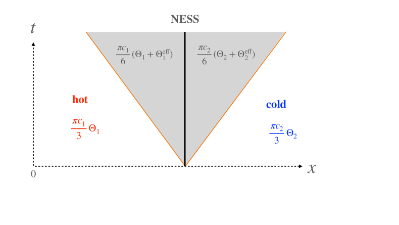
Figure 3: The entropy densities in the four regions of the partitioning protocol discussed in the text (space is here unfolded). The entropies of the outgoing fluids, which depend a priori on details of the scatterer, have been parametrized by two effective temperatures.

The entanglement between outgoing excitations is encoded in a scattering matrix, which we may write schematically as

$$\mathbb{S}(\psi_{1}^{\rm in},\psi_{2}^{\rm in},\psi_{\rm def}^{\rm in}\,|\,\psi_{1}^{\rm out},\psi_{2}^{\rm out},\psi_{\rm def}^{\rm out})\ .$$ (3.9)

Here $\psi_{j}^{\rm in/out}$ are the incoming and outgoing excitations, and $\psi_{\rm def}^{\rm in/out}$ is the state of the defect before/after the scattering. Strictly speaking there is no genuine S-matrix in conformal field theory. What describes the conformal interface is a formal operator ${\mathcal{I}}$, obtained by unfolding the associated boundary state [9, 42]. The above $\mathbb{S}$ is an appropriate Wick rotation of ${\mathcal{I}}$, as explained in ref.[24].  The density matrix of the outgoing fluids depends a priori on the entire S-matrix, not just on the transport coefficients ${\mathcal{T}}_{j}$ and ${\mathcal{R}}_{j}$.

The second law of thermodynamics bounds the effective temperatures from below since the entropy production (3.8) cannot be negative. The $\Theta_{j}^{\rm eff}$ are also bounded from above because the entropy density cannot exceed the microcanonical one, $s=(\pi c\,u/3)^{1/2}$ with $u$ the energy density of the chiral fluid. Using (3.1) and the detailed-balance condition this gives

$$\Theta_{1}^{{\rm eff}}\leq\sqrt{{\mathcal{R}}_{1}\Theta_{1}^{2}+{\mathcal{T}}_{1}\Theta_{2}^{2}}\qquad{\rm and}\qquad\Theta_{2}^{{\rm eff}}\leq\sqrt{{\mathcal{R}}_{2}\Theta_{2}^{2}+{\mathcal{T}}_{2}\Theta_{1}^{2}}\ \ .$$ (3.10)

The bounds are saturated by perfectly-reflecting or transmitting interfaces, i.e. when either ${\mathcal{R}}_{j}=1$ or ${\mathcal{T}}_{j}=1$. This is trivial, because in such cases there is no entanglement between the outgoing fluids.

Partially reflecting/transmitting interfaces that saturate the bounds (3.10) act as perfect scramblers. Their existence at weak coupling seems unlikely, but strongly-coupled holographic interfaces could be of this kind. We will later argue that the thin-brane holographic interfaces are perfect scramblers. This is supported by the fact (shown in section 6.2) that far from the brane the event horizon approaches the equilibrium BTZ horizons, and hence the outgoing chiral fluids are thermalised.

Any domain-wall solution interpolating between two BTZ geometries, with no other non-trivial asymptotic backgrounds should be likewise dual to a NESS of a perfectly - scrambling interface. We suspect that many top down solutions of this kind exist, but they are hard to find. Indeed, although many BPS domain walls are known in the supergravity literature, their finite-temperature counterparts are rare. The one example that we are aware of is the Janus AdS₃ black brane [43]. But even for this computationally-friendly example the far-from-equilibrium stationary solutions are not known.

4 Stationary branes

To simplify the problem we will here resort to the more tractable thin-brane approximation, hoping that it captures some of the essential physics of the stationary states. This thin-brane holographic model is also the one studied in the related papers [10, 11, 12].

4.1 General setup

Consider two BTZ metrics (2.1) glued along a thin brane whose worldvolume is parametrised by $\tau$ and $\sigma$. Its embedding in the two coordinate patches ($j=1,2$) is given by six functions $\{r_{j}(\tau,\sigma),\,t_{j}(\tau,\sigma),\,x_{j}(\tau,\sigma)\}$. The most general stationary ansatz, such that the induced metric is $\tau$-independent, is of the form

$$x_{j}(\sigma),\ \ r_{j}(\sigma),\ \ t_{j}=\tau+f_{j}(\sigma)\ .$$ (4.1)

In principle one can multiply $\tau$ on the right-hand side by constants $a_{j}^{-1}$. But the metric (2.1) is invariant under rescaling of the coordinates $r\to ar$, $(t,x)\to a^{-1}(t,x)$, and of the parameters $(M,J)\to a^{2}(M,J)$, so we may absorb the $a_{j}$ into a redefinition of the parameters $M_{j},J_{j}$. Hence, without loss of generality, we set $a_{j}=1$.

Following ref.[12] we choose the parameter $\sigma$ to be the redshift factor squared  for a stationary observer

$$\sigma\,=\,r_{1}^{2}-M_{1}\ell_{1}^{2}\,=\,r_{2}^{2}-M_{2}\ell_{2}^{2}\ .$$ (4.2)

With this choice $\hat{g}_{\tau\tau}=-\sigma$  is the same on the two sides of the domain wall, and the functions $r_{j}(\sigma)$ are determined. Of the remaining embedding functions, the sum $f_{1}+f_{2}$ is pure gauge (it can be absorbed by a redefinition of $\tau$) whereas the time delay across the wall, $\Delta t(\sigma)\equiv f_{2}(\sigma)-f_{1}(\sigma)$, is a physically quantity. This and the two functions $x_{j}(\sigma)$ should be determined by solving the three remaining equations: (i) the continuity of the induced-metric components $\hat{g}_{\tau\sigma}$ and $\hat{g}_{\sigma\sigma}$, and (ii) one of the (trace-reversed) Israel-Lanczos conditions 

$$[K_{\alpha\beta}]=-\lambda\,\hat{g}_{\alpha\beta}\ .$$ (4.3)

Here $K_{\alpha\beta}$ is the extrinsic curvature (with $\alpha,\beta\in\{\tau,\sigma\}$), the brackets denote the discontinuity across the wall, and $\lambda$ is the brane tension.

4.2 Solution of the equations

The general local solution of the matching equations is derived in appendix A. The solution is given in the ‘folded setup’ where the interface is a conformal boundary for the product theory CFT${}_{1}\otimes\,$CFT₂. Unfolding side $j$ amounts to sending $x_{j}\to-x_{j}$ and $J_{j}\to-J_{j}$.

The results of appendix A can be summarised as follows. First, from (4.2)

$$r_{j}(\sigma)=\sqrt{\sigma+M_{j}\ell_{j}^{\,2}}\ .$$ (4.4)

Secondly, consistency of the extrinsic-curvature equations imposes

$$J_{1}=-J_{2}\ .$$ (4.5)

This ensures conservation of energy in the CFT, as seen from the holographic dictionary (2.8). Thirdly, matching $\hat{g}_{\tau\sigma}$ from the two sides determines the time delay in terms of the embedding functions $x_{j}$,

$$\Delta t^{\prime}\equiv f_{2}^{\prime}-f_{1}^{\prime}={J_{1}\over 2\sigma}(\ell_{1}x_{1}^{\prime}+\ell_{2}x_{2}^{\prime})\ ,$$ (4.6)

where primes denote derivatives with respect to $\sigma$. What remains is thus to find the functions $x_{j}(\sigma)$.

To this end we use the continuity of $\hat{g}_{\sigma\sigma}$ and the $\tau\tau$ component of (4.3). It is useful and convenient to first solve these two equations for the determinant of the induced metric, with the result

$$-{\rm det}\,\hat{g}\,=\,{\lambda^{2}\sigma\over{A\sigma^{2}+2B\sigma+C}}\,=\,{\lambda^{2}\sigma\over{A(\sigma-\sigma_{+})(\sigma-\sigma_{-})}}\ ,$$ (4.7)

where

$$\sigma_{\pm}={-B\pm\sqrt{B^{2}-AC}\over A}$$ (4.8)

and the coefficients $A,B,C$ read

$$\begin{split}A=(\lambda_{\max}^{2}-\lambda^{2})(\lambda^{2}-\lambda_{\min}^{2}),&\quad B=\lambda^{2}(M_{1}+M_{2})-\lambda_{0}^{2}(M_{1}-M_{2}),\\[4.30554pt] &\hskip-28.45274ptC=-(M_{1}-M_{2})^{2}+\lambda^{2}J_{1}^{2}\ .\end{split}$$ (4.9)

The three critical tensions entering in the above coefficients have been defined previously in refs.[10, 12],

$$\lambda_{\rm min}=\biggl{|}{1\over\ell_{1}}-{1\over\ell_{2}}\biggl{|}\ ,\quad\lambda_{\rm max}={1\over\ell_{1}}+{1\over\ell_{2}}\ ,\quad\lambda_{0}=\sqrt{\lambda_{\rm max}\lambda_{\rm min}}\ .$$ (4.10)

Without loss of generality we assume, as earlier, that $\ell_{1}\leq\ell_{2}$, so the absolute value in $\lambda_{\rm min}$ is superfluous. Note that the expressions (4.7) to (4.9) are the same as the ones for static branes [12] except for the extra term $\lambda^{2}J_{1}^{2}$ in the coefficient $C$.

The determinant of the induced metric can be expressed in terms of $x_{j}$ and $\sigma$ in each chart, $j=1$ and $j=2$. It does not depend on the time-shift functions $f_{j}$, which could be absorbed by a reparametrisation of the metric with unit Jacobian. Having already extracted ${\rm det}\,\hat{g}$, one can now invert these relations to find the $x_{j}^{\prime}$,

$$\frac{x_{1}^{\prime}}{\ell_{1}}=-\frac{{\rm sgn}(\sigma)\big{[}(\lambda^{2}+\lambda_{0}^{2})\,\sigma^{2}\,+(M_{1}-M_{2})\sigma\big{]}}{2(\sigma-\sigma_{+}^{\rm H1})(\sigma-\sigma_{-}^{\rm H1})\sqrt{A\sigma(\sigma-\sigma_{+})(\sigma-\sigma_{-})}}\ ,$$ (4.11)

$$\frac{x_{2}^{\prime}}{\ell_{2}}=-\frac{{\rm sgn}(\sigma)\big{[}(\lambda^{2}-\lambda_{0}^{2})\,\sigma^{2}\,-(M_{1}-M_{2})\sigma\big{]}}{2(\sigma-\sigma_{+}^{\rm H2})(\sigma-\sigma_{-}^{\rm H2})\sqrt{A\sigma(\sigma-\sigma_{+})(\sigma-\sigma_{-})}}\ ,$$ (4.12)

where here

$$\sigma_{\pm}^{{\rm H}j}=-{M_{j}\ell_{j}^{2}\over 2}\pm{1\over 2}\sqrt{M_{j}^{2}\ell_{j}^{4}-J_{j}^{2}\ell_{j}^{2}}\$$ (4.13)

are the points where the outer and inner horizons of the $j$th BTZ metric intersect the domain wall.

Eqs. (4.4) to (4.13) give the general stationary solution of the thin-brane equations for any Lagrangian parameters $\ell_{j}$ and $\lambda$, and geometric parameters $M_{j}$ and $J_{1}=-J_{2}$. The Lagrangian parameters are part of the basic data of the interface CFT, while the geometric parameters determine the CFT state. When $J_{1}=J_{2}=0$, all these expressions reduce to the static solutions found in ref.[12].

5 Inside the ergoregion

The qualitative behaviour of the domain wall is governed by the singularities of (4.11, 4.12), as one moves from the AdS boundary at $\sigma\sim\infty$ inwards. In addition to the BTZ horizons at $\sigma^{{\rm H}j}_{\pm}$, other potential singularities arise at $\sigma_{\pm}$ and at the entrance of the ergoregion $\sigma=0$. From (4.7) we see that the brane worldvolume would become spacelike beyond $\sigma=0$, if $\sigma_{\pm}$ are both either negative or complex. To avoid such pathological behaviour one of the following two conditions must be met:

• $\,\sigma_{+}>0\,:$ The singularity at $\sigma_{+}$ is in this case a turning point, and the
  wall does not extend to lower values of $\sigma$. Indeed, as seen from (4.11) and (4.12), $dr_{j}/dx_{j}|_{\sigma_{+}}=0$ and the $\sigma_{+}$ singularity is integrable, i.e. the wall turns around at finite $x_{j}=\int x_{j}^{\prime}$ .

• $\,0=\sigma_{+}>\sigma_{-}\,:$ In this case the worldvolume remains timelike as the wall enters the ergoregion. The reader can verify from eqs. (4.7), (4.11) and (4.12) that the embedding near $\sigma=0$ is smooth.

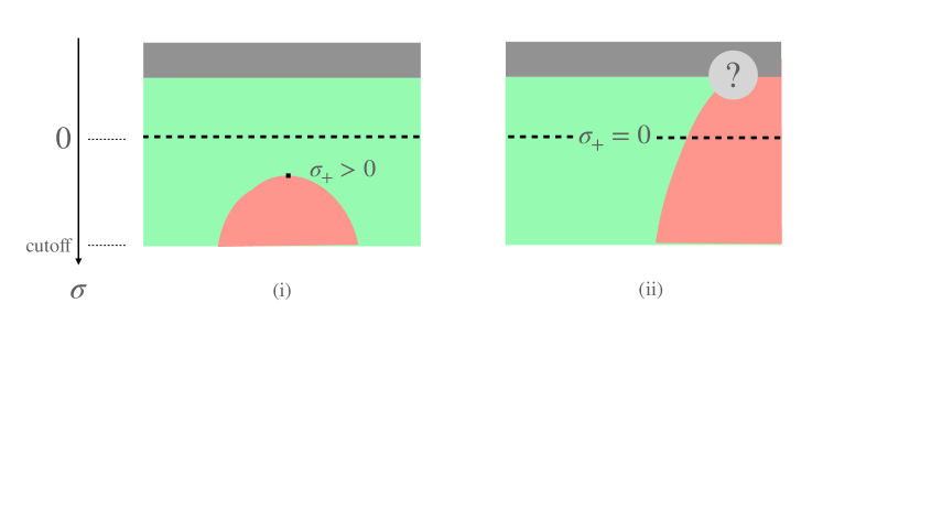
Figure 4: The two kinds of stationary-wall geometries: (i) The wall avoids the ergoregion, turns around and intersects the AdS boundary twice; or (ii) it enters the ergoregion and does not come out again. The broken line is the ergoplane, the two outer BTZ regions are coloured in green and pink, and the region behind the horizon in grey. The horizon in case (ii) will be described in detail in the coming section.

These two possibilities are illustrated in figure 4. Branes entering the ergoregion are dual, as will become clear, to steady states of an isolated interface, while those that avoid the ergoregion are dual to steady states of an interface-antiinterface pair. We will return to the second case in section 7, here we focus on the isolated interface.

The condition $\sigma_{+}=0$ implies $C=0$ and $B\geq 0$. Using eqs. (4.8) and (4.9), and the fact that the coefficient $A$ is positive for tensions in the allowed range ($\lambda_{\min}<\lambda<\lambda_{\max}$) we obtain

$$M_{1}-M_{2}=\pm\lambda J_{1}=\mp\lambda J_{2}\quad{\rm and}\quad\lambda^{2}(M_{1}+M_{2})\geq\lambda_{0}^{\,2}(M_{1}-M_{2})\ .$$ (5.1)

Furthermore, cosmic censorship requires that $\ell_{j}M_{j}>|J_{j}|$ unless the bulk singularity at $r_{j}=0$ is excised (this is the case in the pink region of the left figure 4). If none of the singularities is excised, the inequality in (5.1) is automatically satisfied and hence redundant.

With the help of the holographic dictionary (2.8) one can translate the expression (5.1) for $M_{1}-M_{2}$ to the language of ICFT. Since the incoming fluxes are thermal,  $T_{--}^{(j)}=\pi^{2}\ell_{j}\Theta_{j}^{2}$  and (2.8) gives

$$M_{j}={4\pi^{2}\Theta_{j}^{2}}-{J_{j}\over\ell_{j}}\ \ \Longrightarrow\ \ M_{1}-M_{2}=4\pi^{2}(\Theta_{1}^{2}-\Theta_{2}^{2})-J_{1}({1\over\ell_{1}}+{1\over\ell_{2}})\ .$$ (5.2)

Combining with eq. (5.1) gives the heat-flow rate

$$J_{1}\,=\,2\langle T^{(1)\,tx}\rangle\ =\ {4\pi^{2}}\big{[}{1\over\ell_{1}}+{1\over\ell_{2}}\pm\lambda\big{]}^{-1}(\Theta_{1}^{2}-\Theta_{2}^{2})\ .$$ (5.3)

This agrees with the ICFT expression (3.4) if we identify the transmission coefficients as follows (recall that $c_{j}=12\pi\ell_{j}$)

$${\mathcal{T}_{j}}={2\over\ell_{j}}\big{[}{1\over\ell_{1}}+{1\over\ell_{2}}\pm\lambda\big{]}^{-1}\ .$$ (5.4)

It is gratifying to find that, for the choice of plus sign, (5.4) are precisely the coefficients ${\mathcal{T}_{j}}$ computed in the linearized approximation in ref. [10]. The choice of sign will be justified in a minute.

Let us pause here to take stock of the situation. We found that (i) the dual of an isolated interface must correspond to a brane that enters the ergoregion, and (ii) that the brane equations determine in this case the flow of heat as expected from the CFT result of [24] and the transmission coefficients derived in [10]. To complete the story, we must make sure that once inside the ergoregion the brane does not come out again. If it did, it would intersect the AdS boundary at a second point, so the solution would not be dual to an isolated interface as claimed.

Inserting $\sigma_{+}=0$ in the embedding functions (4.11, 4.12) we find

$$\begin{split}&\frac{x_{1}^{\prime}}{\ell_{1}}=-\frac{(\lambda^{2}+\lambda_{0}^{2})\,\sigma\,+(M_{1}-M_{2})}{2(\sigma-\sigma_{+}^{\rm H1})(\sigma-\sigma_{-}^{\rm H1})\sqrt{A(\sigma-\sigma_{-})}}\ ,\\[4.30554pt] &\frac{x_{2}^{\prime}}{\ell_{2}}=-\frac{(\lambda^{2}-\lambda_{0}^{2})\,\sigma\,-(M_{1}-M_{2})}{2(\sigma-\sigma_{+}^{\rm H2})(\sigma-\sigma_{-}^{\rm H2})\sqrt{A(\sigma-\sigma_{-})}}\ ,\end{split}$$ (5.5)

where the $\sigma_{\pm}^{{\rm H}j}$ are given by eq. (4.13) and

$$\sigma_{-}=-\,{2\lambda\over A}\big{[}\lambda(M_{1}+M_{2})\pm 2\lambda_{0}^{2}J_{1}\big{]}\ .$$ (5.6)

As already said, the embedding is regular at $\sigma=0$, i.e. the brane enters the ergoregion smoothly. What it does next depends on which singularity it encounters first. If this were the square-root singularity at $\sigma_{-}$ , the wall would turn around (just like it does for positive $\sigma_{+}$), exit the ergoregion and intersect the AdS boundary at another anchor point. This is the possibility that we want to exclude.

Consider for starters the simpler case $\ell_{1}=\ell_{2}\equiv\ell$. In this case $\lambda_{0}=0$ and $A=\lambda^{2}(4/\ell^{2}-\lambda^{2})$, so (5.6) reduces to

$$\sigma_{-}\,=\,-{2\ell^{2}\,(M_{1}+M_{2})\over 4-\lambda^{2}\ell^{2}}\ \leq\ -{\rm min}(M_{j})\,\ell^{2}\ .$$ (5.7)

In the last step we used the fact that both $M_{j}$ are positive, otherwise the conical singularity at $r_{j}=0\Longleftrightarrow\sigma=-M_{j}\ell^{2}$ would be naked. What (5.7) shows is that the putative turning point $\sigma_{-}$ lies behind the bulk singularity in at least one of the two BTZ regions, where our solution cannot be extended. Thus this turning point is never reached.

For general $\ell_{1}\not=\ell_{2}$ a weaker statement is true, namely that $\sigma_{-}$ is shielded by an inner horizon for at least one $j$. The proof requires maximising $\sigma_{-}$ with respect to the brane tension $\lambda$. We have performed this calculation with Mathematica, but do not find it useful to reproduce the nitty gritty details here. The key point for our purposes is that there are no solutions in which the brane enters the ergoregion, turns around before an inner horizon, and exits towards the AdS boundary. Since as argued by Penrose [44], Cauchy (inner) horizons are classically unstable, solutions in which the turning point lies behind one of them cannot be trusted.

One last remark is in order concerning the induced brane metric $\hat{g}_{\alpha\beta}$. By redefining the worldvolume time, $\tilde{\tau}=\tau+{J\ell_{1}}\int{x_{1}^{\prime}(\sigma)}d\sigma/{2\sigma}$, we can bring this metric to the diagonal form

$$d\hat{s}^{2}=-\sigma d{\tilde{\tau}}^{2}+|{\rm det}\,\hat{g}|\,\frac{d\sigma^{2}}{\sigma}\qquad{\rm with}\qquad{\rm det}\,\hat{g}={\lambda^{2}\over{A(\sigma_{-}-\sigma)}}\ .$$ (5.8)

The worldvolume is timelike for all $\sigma>\sigma_{-}$, as already advertised. More interestingly, the metric (felt by signals that propagate on the brane) is that of a two-dimensional black-hole with horizon at the ergoplane $\sigma=0$. This lies outside the bulk horizons $\sigma_{+}^{{\rm H}j}$, in agreement with arguments showing that the causal structure is always set by the Einstein metric [50]. Similar remarks in a closely-related context were made before in ref.[51]. The brane-horizon (bH) temperature,

$$4\pi\Theta_{\rm bH}=\big{(}-{\rm det}\,\hat{g}|_{\sigma=0}\big{)}^{-1/2}\ ,$$ (5.9)

is intermediate between $\Theta_{1}$ and $\Theta_{2}$ as can be easily checked. For $\ell_{1}=\ell_{2}$ for example one finds $2\,\Theta_{\rm bH}^{2}=\Theta_{1}^{2}+\Theta_{2}^{2}$.

6 The non-Killing horizon

Since $\sigma_{-}$ lies behind an inner horizon, the first singularities of the embedding functions (5.5) are at $\sigma_{+}^{{\rm H}j}$. A key feature of the non-static solutions is that these outer BTZ horizons, which are apparent horizons as will become clear, do not meet at the same point on the brane. For $J_{j}\not=0$ the following strict inequalities indeed hold

$$\sigma_{+}^{{\rm H}1}>\sigma_{+}^{{\rm H}2}\quad{\rm if}\ \ M_{1}>M_{2}\,;\qquad\,\sigma_{+}^{{\rm H}2}<\sigma_{+}^{{\rm H}1}\quad{\rm if}\ \ M_{1}<M_{2}\ .$$ (6.1)

For small $J_{j}$ these inequalities are manifest by Taylor expanding (4.13),

$$\sigma_{+}^{{\rm H}j}=-{J_{j}^{2}\over M_{j}}+O(J_{j}^{\,4})\ .$$ (6.2)

We show that they hold for all $J_{j}$ in appendix B.

The meaning of these inequalities becomes clear if we use the holographic dictionary (2.8), the energy currents (3.1) and the detailed-balance condition (3.2) to write the $M_{j}$ as follows

$$\begin{split}&M_{1}=2\pi^{2}\left[\Theta_{1}^{2}(1+{\mathcal{R}}_{1})+\Theta_{2}^{2}(1-{\mathcal{R}}_{1})\right]\ ;\\[4.30554pt] &\,\,M_{2}=2\pi^{2}\left[\Theta_{1}^{2}(1-{\mathcal{R}}_{2})+\Theta_{2}^{2}(1+{\mathcal{R}}_{2})\right]\ .\end{split}$$ (6.3)

Assuming $0\leq{\mathcal{R}}_{j}\leq 1$, we see that the hotter side of the interface has the larger $M_{j}$. What (6.1) therefore says is that the brane hits the BTZ horizon of the hotter side first.

6.1 The arrow of time

Assume for concreteness $M_{1}>M_{2}$, the case $M_{2}>M_{1}$ being similar. From eq.(5.1) we have $M_{1}=M_{2}+\lambda|J_{1}|$. We do not commit yet on the sign of $J_{1}$, nor on the sign in eq. (5.1), but the product of the two should be positive. Figure 5 shows the behaviour of the brane past the ergoplane. The vertical axis is parameterised by $\sigma$ (increasing downwards), and the horizontal axes by the ingoing Eddington-Finkelstein coordinates $y_{j}$ defined in eq. (2.4). These coordinates are regular at the future horizons, and reduce to the flat ICFT coordinates $x_{j}$ at the AdS boundary.

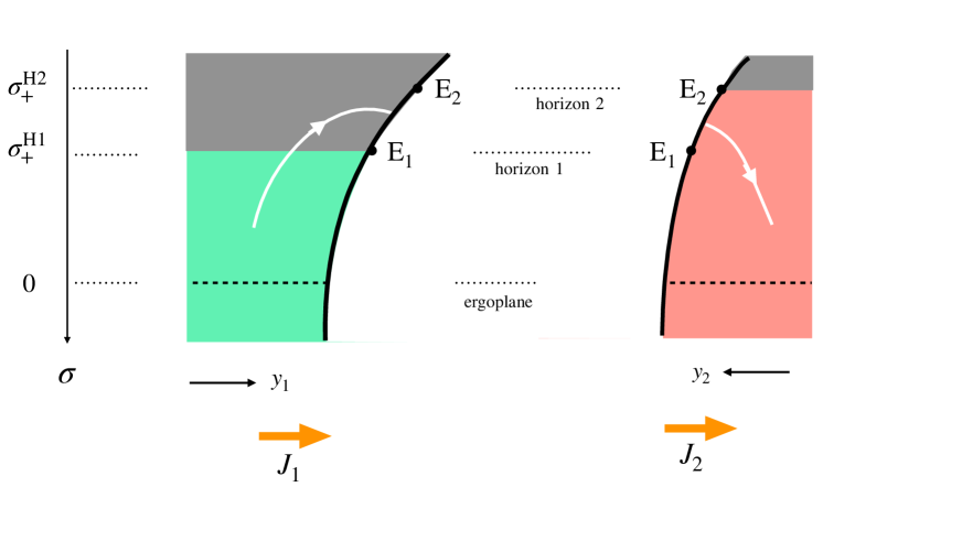
Figure 5: A brane (thick black curve) entering the local outer horizons ${\mathcal{H}}1$ and ${\mathcal{H}}2$ (the boundaries of the grey regions in the figure) at two different points E1 and E2. The piece [E1,E2] of the wall is behind the horizon of slice 1 but outside the horizon of slice 2. The thick orange arrows show the direction of heat flow. The white curve is the worldline of an observer entering ${\mathcal{H}}1$, crossing the brane and emerging outside ${\mathcal{H}}2$.

Let us take a closer look at the wall embedding in Eddington-Finkelstein (EF) coordinates. From eqs. (5.5) and the identities $r_{j}^{\prime}=1/2r_{j}$  we get

$$\begin{split}&y_{1}^{\prime}=\frac{\ell_{1}}{2(\sigma-\sigma_{+}^{\rm H1})(\sigma-\sigma_{-}^{\rm H1})}\left[{J_{1}\ell_{1}\over 2\sqrt{\sigma+M_{1}\ell_{1}^{2}}}-\,\frac{(\lambda^{2}+\lambda_{0}^{2})\,\sigma\,+\lambda|J_{1}|}{\sqrt{A(\sigma-\sigma_{-})}}\right]\ ,\\[4.30554pt] &\,\,y_{2}^{\prime}=\frac{\ell_{2}}{2(\sigma-\sigma_{+}^{\rm H2})(\sigma-\sigma_{-}^{\rm H2})}\left[{J_{2}\ell_{2}\over 2\sqrt{\sigma+M_{2}\ell_{2}^{2}}}-\,\frac{(\lambda^{2}-\lambda_{0}^{2})\,\sigma\,-\lambda|J_{2}|}{\sqrt{A(\sigma-\sigma_{-})}}\right]\ .\end{split}$$ (6.4)

A little algebra shows that the square brackets in the above expression vanish at the corresponding horizons $\sigma=\sigma_{+}^{{\rm H}j}$ if $J_{1}=-J_{2}>0$. The functions $y_{j}$ are in this case analytic at the horizons. By contrast, if $J_{1}=-J_{2}<0$ these functions are singular: $y_{1}\to+\infty$ at $\sigma_{+}^{{\rm H}1}$,  and $y_{2}\to-\infty$ at $\sigma_{+}^{{\rm H}2}$. We interpret this as evidence that $J_{1}$ must be positive, as expected from the arrow of heat flow in the boundary ICFT. This means that $M_{1}=M_{2}+\lambda J_{1}$, and hence the sign in the expression (5.4) for the transmission coefficients is also plus, in agreement with the result of ref. [10].

Note that time reversal flips the sign of the $J_{j}$ and leaves $M_{j}$ unchanged. Since time reversal is a symmetry of the equations, both signs of $J_{1}$ give therefore solutions – one diverging in the past and the other in the future horizons. One can check for consistency that choosing the minus sign in the expressions (5.4) interchanges the incoming and outgoing energy currents in (3.1). Similarly to a white hole, which solves Einstein’s equations but cannot be produced by gravitational collapse, we expect that no physical protocol can prepare the $J_{1}<0$ solution.

6.2 Event versus apparent horizon

Denote by ${\mathcal{H}}_{1}$ and ${\mathcal{H}}_{2}$ the horizons of the two BTZ regions of the stationary geometry, and by E₁ and E₂ their intersections with the brane worldvolume. We can foliate spacetime by Cauchy slices $v_{j}=\bar{v}+\epsilon_{j}(r_{j},x_{j})$, where $\bar{v}$ is a uniform foliation parameter. We use the same symbols for the projections of ${\mathcal{H}}_{j}$ and E_j on a Cauchy slice. Since simultaneous translations of $v_{j}$ are Killing isometries, the projections do not depend on $\bar{v}$.

Both ${\mathcal{H}}_{1}$ and ${\mathcal{H}}_{2}$ are local (or apparent) horizons, i.e. future-directed light rays can only traverse them in one direction. But it is clear from figure 5 that ${\mathcal{H}}_{1}$ cannot be part of the event horizon of global spacetime. Indeed, after entering ${\mathcal{H}}_{1}$ an observer moving to the right can traverse the [E₁, E₂] part of the wall, emerge outside ${\mathcal{H}}_{2}$ in region 2, and from there continue her journey to the boundary. Such journeys are only forbidden if E₁= E₂, i.e. for the static equilibrium solutions.

In order to analyse the problem systematically, we define an everywhere-timelike unit vector field that distinguishes the past from future,

$$t^{\mu}\partial_{\mu}={\partial\over\partial v_{j}}+\,{h_{j}(r_{j})-1\over 2\ell_{j}}\,{\partial\over\partial r_{j}}+{J_{j}\ell_{j}\over 2r_{j}^{2}}\,{\partial\over\partial y_{j}}\qquad{\rm in\ the\ {\it j}th\ region\,.}$$ (6.5)

Using the metric (2.5) the reader can check that $t^{\mu}t_{\mu}=-1$. To avoid charging the formulae we drop temporarily the index $j$. A future-directed null curve has tangent vector

$$\dot{x}^{\mu}=(\dot{v},\dot{r},\dot{y})\ \qquad{\rm where}\quad\dot{x}^{\mu}\dot{x}_{\mu}=0\ \ \ {\rm and}\ \ \ \dot{x}^{\mu}t_{\mu}<0\ .$$ (6.6)

The dots denote derivatives with respect to a parameter on the curve. Solving the conditions (6.6) gives

$$\dot{r}={h\over 2\ell}\dot{v}-{r^{2}\over 2\ell\dot{v}}\bigl{(}\dot{y}-{J\ell\over 2r^{2}}\dot{v}\bigr{)}^{2}\ \quad{\rm and}\ \ \ \dot{v}>0\ .$$ (6.7)

We see that the arrow of time is defined by increasing $v$, and that behind the horizon, where $h(r)$ is negative, $r$ is monotone decreasing with time. This suffices to show that ${\mathcal{H}}_{2}$ is part of the event horizon – an observer crossing it will never make it out to the boundary again.

As explained above, the story differs in region 1. Here the event horizon consists of a lightlike surface $\widetilde{\mathcal{H}}_{1}$ such that no future-directed causal curve starting from a point behind it can reach the [E₁,E₂] part of the wall. Clearly, the global event horizon

$${\mathcal{H}}_{\rm event}=\widetilde{\mathcal{H}}_{1}\,\cup\,{\mathcal{H}}_{2}$$ (6.8)

must be continuous and lie behind the apparent horizon ${\mathcal{H}}_{1}$ in region 1. This is illustrated in figure 6. General theorems [23] actually show that a local horizon which is part of a trapped compact surface cannot lie outside the event horizon. But there is no clash with these theorems here because ${\mathcal{H}}_{1}$ fails to be compact, both at infinity and at E₁.

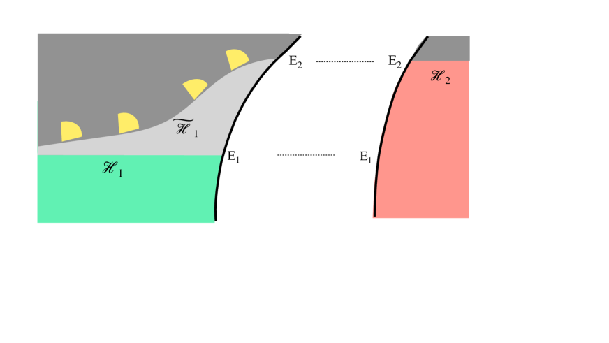
Figure 6: The event and apparent horizons, $\widetilde{\mathcal{H}}_{1}\cup{\mathcal{H}}_{2}$ and ${\mathcal{H}}_{1}\cup{\mathcal{H}}_{2}$, as described in the text. The event horizon is connected but it is not Killing. Projections of the local light-cone on a Cauchy slice are shown in yellow. The light grey region behind ${\mathcal{H}}_{1}$ is outside the event horizon because signals can escape towards the right.

To compute the projection of $\widetilde{\mathcal{H}}_{1}$ on a Cauchy slice, note that it is a curve through the point E₂ that is everywhere tangent to the projection of the local light cone, as shown in the figure. Put differently, at every point on the curve we must minimise the angle between (the projection of) light-like vectors and the positive-$y_{1}$ axis. This will guarantee that an observer starting behind $\widetilde{\mathcal{H}}_{1}$ will not be able to move fast enough towards the right in order to hit the wall before the point E₂.

Parametrising the curve by $y_{1}$, using eq. (6.7) and dropping again for simplicity the $j=1$ index we find

$$-{dy\over dr}\,\bigg{|}_{\widetilde{\mathcal{H}}_{1}}\ =\ {\rm max}_{\,v_{y}>0}\ \bigg{[}{r^{2}\over 2\ell v_{y}}\bigl{(}1-{J\ell\over 2r^{2}}{v_{y}}\bigr{)}^{2}-{h\over 2\ell}{v_{y}}\bigg{]}^{-1}\ ,$$ (6.9)

where $v_{y}\equiv dv/dy$. The extrema of this expression are $v_{y}=\pm r/\sqrt{M\ell^{2}-r^{2}}$. Recall that we are interested in the region behind the BTZ horizon and in future-directed light rays for which $v$ is monotone increasing (whereas $r$ is monotone decreasing). For null rays moving to the right we should thus pick the positive $v_{y}$ extremum. Inserting in (6.9) gives the differential equation obeyed by $\widetilde{\mathcal{H}}_{1}$,

$${dy\over dr}\,\bigg{|}_{\widetilde{\mathcal{H}}1}\ =\ {2\ell\over J\ell-2r\sqrt{M\ell^{2}-r^{2}}}\ \ .$$ (6.10)

The (projected) event horizon in region $j=1$ is the integral of (6.10) with the constant of integration fixed so that the curve passes through E₂.

Here now comes the important point. The reader can check that near the BTZ horizon, $r=r_{+}^{\rm H1}(1+\epsilon)$ with $\epsilon\ll 1$, the denominator in (6.10) vanishes like $1/\epsilon$. This is a non-integrable singularity, so $y(r)$ diverges at $r_{+}^{\rm H1}$ and hence ${\widetilde{\mathcal{H}}1}$ approaches asymptotically ${\mathcal{H}}1$ as announced in section 3.2. The holographic coarse-grained entropy will therefore asymptote to that of the equilibrium BTZ horizon, given by eqs. (2.11) and (2.12). This shows that the chiral outgoing fluid is thermal, not only in the cold region 2 but also in the hotter region 1.

6.3 Remark on flowing funnels

The fact that outgoing fluxes are thermalised means that, in what concerns the entropy and energy flows, the interface behaves like a black cavity. This latter can be modelled by a non-dynamical, two-sided boundary black hole whose (disconnected) horizon consists of two points. To mimic the behaviour of the interface, the two horizon temperatures should be equal to the $\Theta_{j}^{\rm eff}$ that saturate the bounds (3.10). This is illustrated in figure 7.

Figure 7: A two-sided flowing funnel that can mimic the energy and entropy flows of the holographic interface. Tuning the horizon temperatures so that the boundary black hole does not absorb any energy is, however, an adhoc condition.

The precise shape of the flowing horizon(s) depends on the boundary black hole(s) and is not important for our purposes here. For completeness, following ref.[15], we outline how to derive it in appendix C. Like the thin-brane horizon of figure 6, it approaches the BTZ horizons at infinity but differs in the central region (notably with a delta-function peak in the entropy density at $x=0$, see appendix C).

The key difference is however elsewhere. The two halves of the flowing funnel of figure 7 are a priori separate solutions, with the temperatures $\Theta_{j}$ and $\Theta_{j}^{\rm eff}$ chosen at will. But to mimic the conformal interface one must impose continuity of the heat flow,

$${dQ_{1}\over dt}={\pi c_{1}\over 12}(\Theta_{1}^{2}-(\Theta_{1}^{\rm eff})^{2})={\pi c_{2}\over 12}((\Theta_{2}^{\rm eff})^{2}-\Theta_{2}^{2})={dQ_{2}\over dt}\ .$$ (6.11)

This relates the horizon temperatures to each other and to those of the distant heat baths. It is however unclear whether any local condition behind the event horizons can impose the condition (6.11) .

7 Pair of interfaces

In this last section we consider a pair of identical interfaces between two theories, CFT₁ and CFT₂. The interface separation is $\Delta x$. Let the theory that lives in the finite interval be CFT₂ and the theory outside be CFT₁ (recall that we are assuming $\ell_{2}\geq\ell_{1}$). At thermal equilibrium the system undergoes a first-order phase transition at a critical temperature $\Theta_{\rm cr}=b/\Delta x$ where $b$ depends on the classical Lagrangian parameters $\lambda\ell_{j}$ [12, 11]. Below $\Theta_{\rm cr}$ the brane avoids the horizon and is connected, while above $\Theta_{\rm cr}$ it breaks into two disjoint pieces that hit separately the singularity of the black hole. This is a variant of the Hawking-Page phase transition [52] that can be interpreted [53] as a deconfinement transition of CFT₂.

We would like to understand what happens when this system is coupled to reservoirs with slightly different temperatures $\Theta_{\pm}=\Theta\pm d\Theta$ at $x=\pm\infty$. Because of the temperature gradient the branes are now stationary, but they conserve the topology of their static ancestors. In the low-$\Theta$ phase the brane avoids the ergoregion (which is displaced from the horizon infinitesimally) and stays connected, while in the high-$\Theta$ phase it splits in two disjoint branes that enter the ergoregion and hit separately a Cauchy horizon or a bulk singularity. The two phases are illustrated in figure 8.

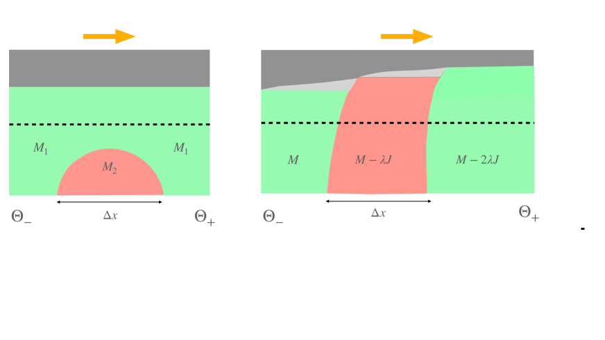
Figure 8: The two types of NESS for an interface pair. In the ’quantum phase’ (left) heat conducts as if there was no scatterer, while in the ’classical phase’ (right) the conductance is the same as for an isolated CFT₁ defect dual to a brane of tension $2\lambda$. Also given in the figure is the BTZ mass parameter in different regions of the geometry. The yellow arrows show the direction of heat flow.

Consider the high-$\Theta$ phase first. The isolated-brane solution of sections 5 and 6 is here juxtaposed to a solution in which the roles of CFT₁ and CFT₂ are inverted. The mass parameter of the three BTZ regions decreases in the direction of heat flow, jumping by $\lambda J$ across each brane. This is indeed the ‘ticket of entry’ to the ergoregion, as explained in eq. (5.1) and section 6.1. The total change of BTZ mass across the pair is the same as if the two branes had merged into a single one with twice the tension. Using the holographic dictionary (2.8) and the fact that incoming fluxes at $x=\pm\infty$ are thermal with temperatures $\Theta_{\pm}$ one indeed computes

$$\underline{{\rm high}\ \Theta}:\qquad{dQ\over dt}\,=\,{\pi^{2}\ell_{1}\over 1+\lambda\ell_{1}}(\Theta^{2}_{-}-\Theta^{2}_{+})\ \equiv\ {\pi^{2}\ell_{1}}{\mathcal{T}}_{\rm pair}(\Theta^{2}_{-}-\Theta^{2}_{+})\,.\ \ \$$ (7.1)

where the effective transmission coefficient ${\mathcal{T}}_{\rm pair}$ is that of a CFT₁ defect whose dual brane has tension $2\lambda$. Note in passing that this effective brane tension can exceed the upper bound (4.10) above which an individual brane inflates, and that an array of widely-spaced branes can make the transmission coefficient arbitrarily small.

The heat flow (7.1) is what one would obtain from classical scatterers. To understand why, think of ${\mathcal{T}}_{j}$ and ${\mathcal{R}}_{j}$ as classical transmission and reflection probabilities for quasi-particles incident on the interface from the side $j$. The probability of passing through both interfaces is the sum of probabilities of trajectories with any number of double reflections in between,

$${\mathcal{T}}_{\rm pair}={\mathcal{T}}_{1}\,(1+{\mathcal{R}}_{2}^{2}+{\mathcal{R}}_{2}^{4}+\cdots)\,{\mathcal{T}}_{2}\,=\,{{\mathcal{T}}_{1}{\mathcal{T}}_{2}\over 1-{\mathcal{R}}_{2}^{2}}={1\over 1+\ell_{1}\lambda}\ ,\ \ \$$ (7.2)

where in the last step we used the holographic relations (5.4). This gives precisely the result (7.1) as advertised.

The low-$\Theta$ case is drastically different. The solution is now obtained by gluing a brane with a turning point (i.e. $\sigma_{+}>0$, see section 4.2) to its mirror image, so that the brane has reflection symmetry. The bulk metric, however, is not $\mathbb{Z}_{2}$ symmetric because in the mirror image we do not flip the sign of the BTZ ‘spin’ $J$. This is required for continuity of the $dxdt$ component of the bulk metric, and it is allowed because when the brane avoids the ergoregion there is no regularity condition to fix the sign of $J$, as in section 6.2. The BTZ mass is thus the same at $x=\pm\infty$, while its value in the CFT₂ region depends on the interface separation $\Delta x$. It follows from the holographic dictionary (2.8) that the heat flow is in this case unobstructed,

$$\underline{{\rm low}\ \Theta}:\qquad{dQ\over dt}\,=\,{\pi^{2}\ell_{1}}(\Theta^{2}_{-}-\Theta^{2}_{+})\,,$$ (7.3)

i.e. the effective transmission coefficient is ${\mathcal{T}}_{\rm pair}=1$. Superficially, it looks as if two branes with equal and opposite tensions have merged into a tensionless one.

In reality, however, the above phenomenon is deeply quantum. What the calculation says is that when a characteristic thermal wavelength becomes larger than the interface separation, coherent scattering results in all incident energy being transmitted. This is all the more surprising since CFT₂ is in the confined phase, and one could have expected that fewer degrees of freedom are available to conduct heat. The microscopic mechanism behind this surprising phenomenon deserves to be studied further.

The above discussion stays valid for finite temperature difference $\Theta_{+}-\Theta_{-}$, but the dominant phase cannot in this case be found by comparing free energies. Nevertheless, as $\Delta x\to 0$ we expect from the dual ICFT that the interface-antiinterface pair fuses into the trivial (identity) defect [42], whereas at very large $\Delta x$ the connected solution ceases to exist. A transition is therefore bound to occur between these extreme separations.

Let us comment finally on what happens if the interval theory is CFT₁, the theory with fewer degrees of freedom, and the outside theory is CFT₂. Here the low-temperature phase only exists for sufficiently-large tension if $c_{1}<c_{2}<3c_{1}$, and does not exist if $c_{2}>3c_{1}$ [12, 11]. The (sparse) degrees of freedom of the interval theory in this latter case are always in the high-temperature phase, and there can be no quantum-coherent conduction of heat. Reassuringly, this includes the limit $c_{2}/c_{1}\to 0$ in which the CFT₁ interval is effectively void.

Note also that in the low-temperature phase the wire can be compactified to a circle and the heat current can be sustained without external reservoirs. This is not possible in the high-temperature phase.

8 Closing remarks

The study of far-from-equilibrium quantum systems is an exciting frontier both in condensed-matter physics and in quantum gravity. Holography is a bridge between these two areas of research, and has led to many new insights. Much remains however to be understood, and simple tractable models can help as testing grounds for new ideas. The holographic NESS of this paper are tractable thanks to several simplifying factors: 2d conformal symmetry, isolated impurities and the assumption of a thin brane. If the first two can be justified in (very) pure ballistic systems, the thin-brane approximation is an adhoc assumption of convenience. Extending our results to top-down dual pairs is one urgent open question.

Another obvious question concerns the structure of entanglement and the Hubeny-Rangamani-Ryu-Takayanagi curves [33, 34] in the above steady states. While it is known that geodesics cannot probe the region behind equilibrium horizons [54], they can reach behind both apparent and event horizons in time-dependent backgrounds, see e.g. [55, 56, 57]. In the framework of the fluid/gravity correspondence the entropy current associated to the event horizon is a local functional of the boundary data [58]. It would be interesting to examine this question in the present far-from-equilibrium context. Note also that the particularly simple form of matter in our problem (a thin fluctuating brane) may allow analytic calculations of the quantum-corrected extremal surfaces [59, 60].

Another interesting question is how the deconfinement transition of the interval CFT in section 7 relates to the sudden jump in thermal conductivity of the system. Last but not least, it would be nice to relate the production of coarse-grained entropy to the scattering matrix of microscopic interfaces, e.g. for the simplest free-field interfaces of [9, 42, 61].

We hope to return to some of these questions in the near future.

Aknowledgements: We thank Denis Bernard, Shira Chapman, Dongsheng Ge, Andreas Karch, Joao Penedones and Giuseppe Policastro for many stimulating discussions during the course of this work. We are indebted to Giuseppe Policastro for the observation that led to the argument around equation (7.2). C.B. also aknowledges the support of the NYU-PSL project ”Holography and Quantum Gravity” (ANR-10-IDEX-0001-02 PSL).

Note added: In more than 1+1 dimensions the two shock waves of figure 1 are replaced by a shockwave on the cold side and a broadening rarefaction wave on the hot side, see [62, 63, 64]. Although this only affects the approach to the NESS in the partitioning protocol, not the NESS proper, it is interesting that the event horizon of our interface NESS follows a similar pattern: it coincides with the equilibrium BTZ horizon on the colder side but approaches it only asymptotically on the hotter side. We thank Julian Sonner, and also Christian Ecker, Johanna Erdmenger and Wilke Van Der Schee for email exchanges on this point.

Appendix A Solving the thin-brane equations

From the form (2.1) of the bulk metric and the embedding ansatz (4.1) of a stationary brane, we derive the following continuity equations for the induced metric

$$\hat{g}_{\tau\tau}\,=\,M_{1}\ell_{1}^{2}-r_{1}^{2}=M_{2}\ell_{2}^{2}-r_{2}^{2}\,,$$ (A.1)

$$\hat{g}_{\tau\sigma}\,=\,(M_{1}\ell_{1}^{2}-r_{1}^{2})f_{1}^{\prime}-{J_{1}\ell_{1}\over 2}x_{1}^{\prime}=(M_{2}\ell_{2}^{2}-r_{2}^{2})f_{2}^{\prime}-{J_{2}\ell_{2}\over 2}x_{2}^{\prime}\,,$$ (A.2)

$${}\hat{g}_{\sigma\sigma}\,= \frac{\ell_{1}^{2}\,r_{1}^{\prime 2}}{h_{1}(r_{1})}+r_{1}^{2}x_{1}^{\prime 2}-J_{1}\ell_{1}x_{1}^{\prime}f_{1}^{\prime}+(M_{1}\ell_{1}^{2}-r_{1}^{2})f_{1}^{\prime 2}$$ (A.3)

$$=\,\frac{\ell_{2}^{2}\,r_{2}^{\prime 2}}{h_{2}(r_{2})}+r_{2}^{2}x_{2}^{\prime 2}-J_{2}\ell_{2}x_{2}^{\prime}f_{2}^{\prime}+(M_{2}\ell_{2}^{2}-r_{2}^{2})f_{2}^{\prime 2}\,.$$

The primes denote derivatives with respect to $\sigma$, and the function $h(r)$ has been defined in eq.(2.3),

$$h(r)\,=\,{r^{2}}-M\ell^{2}+{J^{2}\ell^{2}\over 4r^{2}}\,=\,{1\over r^{2}}(r^{2}-r_{+}^{2})(r^{2}-r_{-}^{2})\ .$$ (A.4)

Following ref.[12] we choose the convenient parametrization $\sigma=-\hat{g}_{\tau\tau}$ , so that $r_{j}^{2}=\sigma+M_{j}\ell_{j}^{2}$  and $r_{j}^{\prime}=1/2r_{j}$. This parametrization need not be one-to-one, it actually only covers half of the wall when this latter has a turning point. With this choice the ergoplane is located at $r_{j}^{2}=M_{j}\ell_{j}^{2}\,\Longrightarrow\,\sigma=0$, and the functions $h_{j}$ can be written as

$$h_{j}(\sigma)={\sigma^{2}+\sigma M_{j}\ell_{j}^{2}+J_{j}^{2}\ell_{j}^{2}/4\over\sigma+M_{j}\ell_{j}^{2}}\ =\ {(\sigma-\sigma_{+}^{{\rm H}j})(\sigma-\sigma_{-}^{{\rm H}j})\over\sigma+M_{j}\ell_{j}^{2}}\ ,$$ (A.5)

where

$$\sigma_{\pm}^{{\rm H}j}=-{M_{j}\ell_{j}^{2}\over 2}\pm{1\over 2}\sqrt{M_{j}^{2}\ell_{j}^{4}-J_{j}^{2}\ell_{j}^{2}}\$$ (A.6)

are the locations of the horizons in the $j$th chart.

From (A.1) - (A.3) one computes the determinant of the induced metric

$$-{\rm det}(\hat{g})\,=\,\frac{\sigma\ell_{j}^{2}}{4r_{j}^{2}h_{j}}+{h_{j}r_{j}^{2}}x_{j}^{\prime\,2}\,.$$ (A.7)

Note that it does not depend on the time-delay functions $f_{j}(\sigma)$, because these can be absorbed by the unit-Jacobian reparametrization

$$\tilde{\tau}=\tau+f_{j}(\sigma),\quad\tilde{\sigma}=\sigma\,.$$

Eq. (A.7) can be used to express the $x_{j}^{\prime}$ (up to a sign) in terms of det $\hat{g}$. A combination of eqs. (A.1) and (A.2) expresses, in turn, the time delay across the wall in terms of the $x_{j}^{\prime}$,

$$\sigma(f_{2}^{\prime}-f_{1}^{\prime})={1\over 2}(J_{1}\ell_{1}x_{1}^{\prime}-J_{2}\ell_{2}x_{2}^{\prime})\ .$$ (A.8)

To complete the calculation we need therefore to find det $\hat{g}$ and then solve the equations (A.7) for $x_{j}^{\prime}$.

The Israel-Lanczos conditions

This is done with the help of the Israel-Lanczos conditions [65, 66] (see also [67]) which express the discontinuity of the extrinsic curvature across the wall, eqs.(4.3). We follow the conventions of ref.[12]: $K_{\alpha\beta}$ is the covariant derivative of the inward-pointing unit normal vector, and the orientation is such that for inceasing $\sigma$ the wall encircles clockwise the interior of both charts in the $(x_{j},r^{-1})$ planes.

A somewhat tedious but straightforward calculation gives

$$K_{\tau\tau}=-\frac{hr^{2}x^{\prime}}{\ell\sqrt{|\hat{g}|}}\qquad{\rm and}\qquad K_{\tau\sigma}=\frac{hr^{2}x^{\prime}}{\sigma\ell\sqrt{|\hat{g}|}}\,\,\hat{g}_{\tau\sigma}+\frac{J\sqrt{|\hat{g}|}}{2\sigma}\ ,$$ (A.9)

where $\hat{g}$ is a shorthand notation for ${\rm det}(\hat{g})$. The Israel-Lanczos equations (4.3) thus read

$${1\over\sqrt{|\hat{g}}|}\Bigl{(}\frac{h_{1}r_{1}^{2}x_{1}^{\prime}}{\ell_{1}}+\frac{h_{2}r_{2}^{2}x_{2}^{\prime}}{\ell_{2}}\Bigr{)}=-\lambda\sigma\,,$$ (A.10)

$${1\over\sqrt{|\hat{g}}|}\Bigl{(}\frac{h_{1}r_{1}^{2}x_{1}^{\prime}}{\ell_{1}}+\frac{h_{2}r_{2}^{2}x_{2}^{\prime}}{\ell_{2}}\Bigr{)}\,\hat{g}_{\tau\sigma}+\frac{\sqrt{|\hat{g}}|}{2}(J_{1}+J_{2})=-\lambda\sigma\,\hat{g}_{\tau\sigma}\,.$$ (A.11)

These are compatible if and only if

$$J_{1}+J_{2}=0\ ,$$ (A.12)

which translates to energy conservation in the boundary CFT. We have checked that the third equation, $[K_{\sigma\sigma}]=-\lambda\hat{g}_{\sigma\sigma}$ , is automatically obeyed and thus redundant. As expected, by virtue of the momentum constraints the three Israel-Lanczos equations (4.3) reduce to a single independent one plus the “constant-of-integration” condition (A.12).

The general solution

Squaring twice (A.10) and using (A.7) to eliminate the $x_{j}^{\prime\,2}$  leads to a quadratic equation for the determinant. This has a singular solution ${\rm det}(\hat{g})=0$, and a non-pathological one

$$-{\rm det}(\hat{g})=\lambda^{2}\sigma^{3}\bigg{[}\frac{4h_{1}h_{2}r_{1}^{2}r_{2}^{2}}{\ell_{1}^{2}\ell_{2}^{2}}-\big{(}\frac{h_{1}r_{1}^{2}}{\ell_{1}^{2}}+\frac{h_{2}r_{2}^{2}}{\ell_{2}^{2}}-\lambda^{2}\sigma^{2}\big{)}^{2}\bigg{]}^{-1}.$$ (A.13)

Inserting the expressions for $r_{j}(\sigma)$ and $h_{j}(\sigma)$ leads after some algebra to

$$-{\rm det}(\hat{g})=\frac{\lambda^{2}\sigma}{A\sigma^{2}+2B\sigma+C}$$ (A.14)

with coefficients

$$\begin{split}&A=(\lambda_{\max}^{2}-\lambda^{2})(\lambda^{2}-\lambda_{\min}^{2})\ ,\\[4.30554pt] &B=\lambda^{2}(M_{1}+M_{2})-\lambda_{0}^{2}(M_{1}-M_{2})\ ,\\[4.30554pt] &C=-(M_{1}-M_{2})^{2}+\lambda^{2}J_{1}^{2}\ .\end{split}$$ (A.15)

The critical tensions in these expressions are

$$\lambda_{\rm min}=\big{|}{1\over\ell_{1}}-{1\over\ell_{2}}\big{|}\ ,\quad\lambda_{\rm max}={1\over\ell_{1}}+{1\over\ell_{2}}\ ,\quad\lambda_{0}=\sqrt{\lambda_{\rm max}\lambda_{\rm min}}\ .$$ (A.16)

For a static wall, i.e. when $J_{1}=J_{2}=0$, the above formulae reduce, as they should, to the ones obtained in ref.[12].  The only effect of the non-zero $J_{j}$ is actually to shift the coefficient $C$ in (A.15).

The roots of the quadratic polynomial in the denominator of (A.14),

$$\sigma_{\pm}={-B\pm\sqrt{B^{2}-AC}\over A}\ ,$$ (A.17)

determine the behaviour of the solution. If $\sigma_{+}$ is either complex or negative (part of) the brane worldvolume has ${\rm det}\,\hat{g}>0$ in the ergoregion, so it is spacelike and physically unacceptable. Acceptable solutions have $\sigma_{+}>0$ or $\sigma_{+}=0$, and describe walls that avoid, respectively enter the ergoregion as explained in the main text, see section 5.

The actual shape of the wall is found by inserting (A.14) in (A.7) and solving for $x_{j}^{\prime\,2}$. After some rearrangements this gives

$$\epsilon_{1}\frac{x_{1}^{\prime}}{\ell_{1}}=\frac{(\lambda^{2}+\lambda_{0}^{2})\sigma+(M_{1}-M_{2})}{2(\sigma+M_{1}\ell_{1}^{2}+J^{2}\ell_{1}^{2}/4\sigma)\sqrt{A\sigma(\sigma-\sigma_{+})(\sigma-\sigma_{-})}}\ ,$$ (A.18)

$$\epsilon_{2}\frac{x_{2}^{\prime}}{\ell_{2}}=\frac{(\lambda^{2}-\lambda_{0}^{2})\sigma-(M_{1}-M_{2})}{2(\sigma+M_{2}\ell_{2}^{2}+J^{2}\ell_{2}^{2}/4\sigma)\sqrt{A\sigma(\sigma-\sigma_{+})(\sigma-\sigma_{-})}}\ ,$$ (A.19)

where $\epsilon_{j}=\pm$ are signs. They are fixed by the linear equation (A.10) with the result

$$\epsilon_{j}(\sigma)=-{\sigma\over|\sigma|}\ .$$ (A.20)

These signs agree with the known universal solution [68, 12] near the AdS boundary, at $\sigma\to\infty$, and they ensure that walls entering the ergoregion have no kink. Expressing the denominators in terms of the horizon locations (A.6) gives the equations (4.11) and (4.12) of the main text.

It is worth noting that the tensionless ($\lambda\to 0$) limit of our solution is singular. Indeed, on one hand extremising the brane action and ignoring its back-reaction gives a geodesic worldvolume, but on the other hand for $\lambda=0$ fluctuations of the string are unsuppressed. In fact, when $\lambda$ is small the wall starts as a geodesic near the AdS boundary but always departs significantly in the interior. In particular, a geodesic never enters the equilibrium horizon, whereas a tensile string can, even if it is very light.

Appendix B Horizon inequalities

In section 6 we asserted that BTZ geometries whose ergoregions can be glued together by a thin brane obey the inequalities

$$\sigma_{+}^{{\rm H}1}>\sigma_{+}^{{\rm H}2}\quad{\rm if}\ \ M_{1}>M_{2}\,;\qquad\,\sigma_{+}^{{\rm H}2}<\sigma_{+}^{{\rm H}1}\quad{\rm if}\ \ M_{1}<M_{2}\ ,$$ (B.1)

where the horizon locations are

$$\sigma_{\pm}^{{\rm H}j}=-{M_{j}\ell_{j}^{2}\over 2}\pm{1\over 2}\sqrt{M_{j}^{2}\ell_{j}^{4}-J^{2}\ell_{j}^{2}}\$$ (B.2)

and $J\equiv|J_{1}|=|J_{2}|>0$. This ordering of the outer horizons is manifest if one expands at the leading order for small $J$. We want to show that it is valid for all values of $J$.

If as $J$ is cranked up the ordering was at some point reversed, then at this point we would have $\sigma_{+}^{{\rm H}1}=\sigma_{+}^{{\rm H}2}$, or equivalently

$$M_{2}\ell_{2}^{2}-M_{1}\ell_{1}^{2}=\sqrt{M_{2}^{2}\ell_{2}^{4}-J^{2}\ell_{2}^{2}}-\sqrt{M_{1}^{2}\ell_{1}^{4}-J^{2}\ell_{1}^{2}}\ .$$ (B.3)

Squaring twice to eliminate the square roots gives

$$J^{\,2}=\frac{4\ell_{1}^{2}\ell_{2}^{2}(M_{1}-M_{2})(M_{2}\ell_{2}^{2}-M_{1}\ell_{1}^{2})}{(\ell_{2}^{2}-\ell_{1}^{2})^{2}}\ .$$ (B.4)

Without loss of generality we assume, as elsewhere in the text, that $\ell_{1}\leq\ell_{2}$. If $M_{2}>M_{1}$, then automatically $M_{2}\ell_{2}^{2}>M_{1}\ell_{1}^{2}$ and (B.4) has no solution for real $J$. In this case the ordering (B.1) cannot be reversed.

If on the other hand $M_{1}>M_{2}$ and $M_{2}\ell_{2}^{2}-M_{1}\ell_{1}^{2}>0$ we need to work harder. Inserting $J^{2}$ from (B.4) back in the original equation (B.3) gives after rearrangements

$$(\ell_{2}^{2}-\ell_{1}^{2})(M_{2}\ell_{2}^{2}-M_{1}\ell_{1}^{2})\,= \ell_{2}^{2}\,\bigl{|}(M_{2}\ell_{2}^{2}-M_{1}\ell_{1}^{2})-\ell_{1}^{2}(M_{1}-M_{2})\bigr{|}$$ (B.5)

$$-\ell_{1}^{2}\left|(M_{2}\ell_{2}^{2}-M_{1}\ell_{1}^{2})-\ell_{2}^{2}(M_{1}-M_{2})\right|\ ,$$

where the absolute values come from the square roots. This equation is not automatically obeyed whenever its doubly-squared version is. A solution only exists if

$$M_{1}-M_{2}\,\leq\,\frac{\ell_{2}^{2}M_{2}-\ell_{1}^{2}M_{1}}{\ell_{2}^{2}}\ \Leftrightarrow\ \frac{M_{1}}{M_{2}}\,\leq\,\frac{2\ell_{2}^{2}}{\ell_{2}^{2}+\ell_{1}^{2}}\ \ .$$ (B.6)

Remember now that we only care about solutions with walls in the ergoregion, for which $M_{1}-M_{2}=\lambda J$, see eq.(5.1). Plugging in (B.4) this gives

$$M_{2}=\bigl{[}1-\frac{4\lambda_{0}^{2}\,\lambda^{2}}{\lambda_{0}^{\,4}+4{\lambda^{2}}/{\ell_{1}^{2}}}\bigr{]}M_{1}$$ (B.7)

with $\lambda_{0}^{2}=(\ell_{2}^{2}-\ell_{1}^{2})/\ell_{1}^{2}\ell_{2}^{2}$ , see eq.(4.10). Consistency with the bound (B.6) for a brane tension in the allowed range then requires

$$\lambda_{\rm min}<\lambda\,\leq\,\frac{\ell_{1}\lambda_{0}^{2}}{2}\ ,$$ (B.8)

where $\lambda_{\rm min}=(\ell_{2}-\ell_{1})/\ell_{1}\ell_{2}$. As one can easily check, this implies $\ell_{1}>\ell_{2}$ which contradicits our initial assumption. We conclude that (B.3) has no solutiion, and the ordering (B.1) holds for all $J$, QED.

For completeness, let us also consider the ordering of the inner horizons. Clearly $\sigma_{+}^{{\rm H}j}>\sigma_{-}^{{\rm H}j}$ always, and for small $J$ also $\sigma_{+}^{{\rm H}1}>\sigma_{-}^{{\rm H}2}$ and $\sigma_{+}^{{\rm H}2}>\sigma_{-}^{{\rm H}1}$. To violate these last inequalities we need $\sigma_{+}^{{\rm H}1}=\sigma_{-}^{{\rm H}2}$ or $\sigma_{+}^{{\rm H}2}=\sigma_{-}^{{\rm H}1}$ for some finite $J$, or equivalently

$$M_{2}\ell_{2}^{2}-M_{1}\ell_{1}^{2}=\mp\bigl{(}\sqrt{M_{2}^{2}\ell_{2}^{4}-J^{2}\ell_{2}^{2}}+\sqrt{M_{1}^{2}\ell_{1}^{4}-J^{2}\ell_{1}^{2}}\,\bigr{)}\ .$$ (B.9)

Squaring twice gives back eq.(B.4) which has no solution if $M_{2}>M_{1}$. But if $M_{1}>M_{2}$ and $M_{2}\ell_{2}^{2}-M_{1}\ell_{1}^{2}>0$, solutions to $\sigma_{+}^{{\rm H}2}=\sigma_{-}^{{\rm H}1}$ cannot be ruled out. Indeed, inserting $J$ from (B.4) in (B.9) with the $+$ sign gives

$$(\ell_{2}^{2}-\ell_{1}^{2})(M_{2}\ell_{2}^{2}-M_{1}\ell_{1}^{2})\,= \ell_{2}^{2}\,\bigl{|}(M_{2}\ell_{2}^{2}-M_{1}\ell_{1}^{2})-\ell_{1}^{2}(M_{1}-M_{2})\bigr{|}$$ (B.10)

$$+\ell_{1}^{2}\left|(M_{2}\ell_{2}^{2}-M_{1}\ell_{1}^{2})-\ell_{2}^{2}(M_{1}-M_{2})\right|\ ,$$

which requires that

$$\frac{\ell_{2}^{2}M_{2}-\ell_{1}^{2}M_{1}}{\ell_{2}^{2}}\,\leq\,M_{1}-M_{2}\,\leq\,\frac{\ell_{2}^{2}M_{2}-\ell_{1}^{2}M_{1}}{\ell_{1}^{2}}\ .$$ (B.11)

These conditions are compatible with $M_{1}-M_{2}=\lambda J$ and $\lambda$ in the allowed range, so the outer horizon of slice 2 need not always come before the Cauchy horizon of slice 1.

Finally one may ask if the inner (Cauchy) horizons can join continuously, i.e. if $\sigma_{-}^{{\rm H}1}=\sigma_{-}^{{\rm H}2}$ is allowed. A simple calculation shows that this is indeed possible for $\ell_{2}/\ell_{1}<3$, a critical ratio of central charges that also arose in references [11, 12]. We don’t know if this is a coincidence, or if some deeper reason lurks behind.

Appendix C Background on flowing funnels

In this appendix we collect some formulae on the flowing funnels discussed in section 6.3. We start with the most general asymptotically-locally-AdS₃ solution in Fefferman-Graham coordinates, generalising the Banados geometries (2.6) to arbitrary boundary metric [69]

$$ds^{2}={\ell^{2}dz^{2}\over z^{2}}+{1\over z^{2}}\,g_{\alpha\beta}(x,z)\,dx^{\alpha}dx^{\beta}\ ,$$ (C.1)

where $g_{\alpha\beta}$ is a quartic polynomial in $z$ (written here as a matrix)

$$g(x,z)=\ g_{(0)}+z^{2}g_{(2)}+{z^{4}\over 4}g_{(2)}\,g_{(0)}^{-1}\,g_{(2)}\ .$$ (C.2)

In this equation $g_{(0)}$ is the boundary metric and $g_{(2)}$ is given by

$$g_{(2)\,\alpha\beta}=-{\ell^{2}\over 2}R_{(0)}\,g_{(0)\,\alpha\beta}+{\ell}\,\langle T_{\alpha\beta}\rangle\ ,$$ (C.3)

where $R_{(0)}$ is the Ricci scalar of $g_{(0)}$, and $\langle T_{\alpha\beta}\rangle$ the expectation value of the energy-momentum tensor. This must be conserved, $\nabla^{a}_{(0)}\langle T_{ab}\rangle=0$ , and should obey the trace equation  $g_{(0)}^{ab}\langle T_{ab}\rangle=(c/24\pi)\,R_{(0)}$.

We may take the boundary metric to be that of the Schwarzschild black hole (this differs from the metric in [15], but since it is not dynamical we are free to choose our preferred boundary metric),

$$ds^{2}_{(0)}=-f(x)\,dt^{2}+{dx^{2}\over f(x)}\qquad{\rm with}\quad f(x)={x\over x+a}\ .$$ (C.4)

The horizon at $x=0$ has temperature $\Theta_{S}=(4\pi a)^{-1}$. Using the familiar tortoise coordinates we can write

$$ds^{2}_{(0)}=f(x)(-dt^{2}+dx_{*}^{2})\qquad{\rm where}\quad x_{*}=x+a\log x\ .$$ (C.5)

Let $w^{\pm}=x_{*}\pm t$. The expectation value of the energy-momentum tensor in the black-hole metric can be expressed in terms of $\phi=\log f(x)$ as follows

$$\langle T_{\pm\pm}\rangle={\ell\over 2}\,\big{[}\partial^{2}_{\pm}\phi-{1\over 2}(\partial_{\pm}\phi)^{2}\big{]}+k_{\pm}(w^{\pm})\ ,\quad\langle T_{+-}\rangle=-{\ell\over 2}\,\partial_{+}\partial_{-}\phi\ ,$$ (C.6)

with $k_{\pm}$ arbitrary functions of $w^{\pm}$ that depend on the choice of state. At $x\gg a$ where the metric is flat, $k_{\pm}$ determine the incoming and outgoing fluxes of energy. In a stationary solution these must be constant. If a heat bath at temperature $\Theta_{+}$ is placed at infinity, $k_{+}=\pi^{2}\ell\,\Theta_{+}^{2}$ . The function $k_{-}$, on the other hand, is fixed by requiring that there is no outgoing flux at the Schwarzschild horizon. From

$${\ell\over 2}\,\big{[}\partial^{2}_{\pm}\phi-{1\over 2}(\partial_{\pm}\phi)^{2}\big{]}=-{\ell\,(a^{2}+4ax)\over 16(x+a)^{4}}\,$$ (C.7)

we deduce $\langle T_{--}\rangle|_{x=0}=0\,\Longrightarrow\,k_{-}=\ell/16a^{2}=\pi^{2}\ell\,\Theta_{S}^{2}$ . The outgoing flux at infinity is thermalised at the black hole temperature, as expected.

Inserting the expressions (C.3 - C.7) in eqs. (C.1) and (C.2) gives the flowing-funnel metric in Fefferman-Graham coordinates. These are however singular coordinates, not well adapted for calculating the event horizon as shown in [15]. Following this reference, one can compute the horizon by going to BTZ coordinates – this is possible because all solutions are locally equivalent in three dimensions. The change from any metric (C.1) - (C.2) to local BTZ coordinates has been worked out in ref. [70] (see also [71]) and can be used to compute the black-funnel shapes. A noteworthy feature is that the funnels start vertically inwards at $x=0$ [15] making a delta-function contribution to the area density. Note that figure 7 shows two independent flowing funnels with Schwarzschild temperatures $\Theta_{S}=\Theta_{1}^{\rm eff}$ and $\Theta_{2}^{\rm eff}$.

References

- [1] J. M. Maldacena, “The Large N limit of superconformal field theories and supergravity,” Adv. Theor. Math. Phys. 2 (1998) 231–252, arXiv:hep-th/9711200.
- [2] S. S. Gubser, I. R. Klebanov, and A. M. Polyakov, “Gauge theory correlators from noncritical string theory,” Phys. Lett. B 428 (1998) 105–114, arXiv:hep-th/9802109.
- [3] E. Witten, “Anti-de Sitter space and holography,” Adv. Theor. Math. Phys. 2 (1998) 253–291, arXiv:hep-th/9802150.
- [4] H. Liu and J. Sonner, “Holographic systems far from equilibrium: a review,” arXiv:1810.02367 [hep-th].
- [5] D. Bernard and B. Doyon, “Conformal field theory out of equilibrium: a review,” J. Stat. Mech. 1606 no. 6, (2016) 064005, arXiv:1603.07765 [cond-mat.stat-mech].
- [6] M. Banados, C. Teitelboim, and J. Zanelli, “The Black hole in three-dimensional space-time,” Phys. Rev. Lett. 69 (1992) 1849–1851, arXiv:hep-th/9204099.
- [7] M. Banados, M. Henneaux, C. Teitelboim, and J. Zanelli, “Geometry of the (2+1) black hole,” Phys. Rev. D 48 (1993) 1506–1525, arXiv:gr-qc/9302012. [Erratum: Phys.Rev.D 88, 069902 (2013)].
- [8] A. Karch and L. Randall, “Open and closed string interpretation of SUSY CFT’s on branes with boundaries,” JHEP 06 (2001) 063, arXiv:hep-th/0105132.
- [9] C. Bachas, J. de Boer, R. Dijkgraaf, and H. Ooguri, “Permeable conformal walls and holography,” JHEP 06 (2002) 027, arXiv:hep-th/0111210.
- [10] C. Bachas, S. Chapman, D. Ge, and G. Policastro, “Energy Reflection and Transmission at 2D Holographic Interfaces,” Phys. Rev. Lett. 125 no. 23, (2020) 231602, arXiv:2006.11333 [hep-th].
- [11] P. Simidzija and M. Van Raamsdonk, “Holo-ween,” JHEP 12 (2020) 028, arXiv:2006.13943 [hep-th].
- [12] C. Bachas and V. Papadopoulos, “Phases of Holographic Interfaces,” JHEP 04 (2021) 262, arXiv:2101.12529 [hep-th].
- [13] S. Bhattacharyya and S. Minwalla, “Weak Field Black Hole Formation in Asymptotically AdS Spacetimes,” JHEP 09 (2009) 034, arXiv:0904.0464 [hep-th].
- [14] V. E. Hubeny, D. Marolf, and M. Rangamani, “Hawking radiation in large N strongly-coupled field theories,” Class. Quant. Grav. 27 (2010) 095015, arXiv:0908.2270 [hep-th].
- [15] S. Fischetti and D. Marolf, “Flowing Funnels: Heat sources for field theories and the AdS3 dual of CFT2 Hawking radiation,” Class. Quant. Grav. 29 (2012) 105004, arXiv:1202.5069 [hep-th].
- [16] R. Emparan and M. Martinez, “Black String Flow,” JHEP 09 (2013) 068, arXiv:1307.2276 [hep-th].
- [17] D. Marolf, M. Rangamani, and T. Wiseman, “Holographic thermal field theory on curved spacetimes,” Class. Quant. Grav. 31 (2014) 063001, arXiv:1312.0612 [hep-th].
- [18] J. E. Santos, “To go or not to go with the flow: Hawking radiation at strong coupling,” JHEP 06 (2020) 104, arXiv:2003.05454 [hep-th].
- [19] V. E. Hubeny, S. Minwalla, and M. Rangamani, “The fluid/gravity correspondence,” in Theoretical Advanced Study Institute in Elementary Particle Physics: String theory and its Applications: From meV to the Planck Scale. 7, 2011. arXiv:1107.5780 [hep-th].
- [20] S. W. Hawking, “Black holes in general relativity,” Commun. Math. Phys. 25 (1972) 152–166.
- [21] S. Hollands, A. Ishibashi, and R. M. Wald, “A Higher dimensional stationary rotating black hole must be axisymmetric,” Commun. Math. Phys. 271 (2007) 699–722, arXiv:gr-qc/0605106.
- [22] V. Moncrief and J. Isenberg, “Symmetries of Higher Dimensional Black Holes,” Class. Quant. Grav. 25 (2008) 195015, arXiv:0805.1451 [gr-qc].
- [23] S. W. Hawking and G. F. R. Ellis, The Large Scale Structure of Space-Time. Cambridge Monographs on Mathematical Physics. Cambridge University Press, 2, 2011.
- [24] D. Bernard, B. Doyon, and J. Viti, “Non-Equilibrium Conformal Field Theories with Impurities,” J. Phys. A 48 no. 5, (2015) 05FT01, arXiv:1411.0470 [math-ph].
- [25] M. Meineri, J. Penedones, and A. Rousset, “Colliders and conformal interfaces,” JHEP 02 (2020) 138, arXiv:1904.10974 [hep-th].
- [26] S. Carlip, “The (2+1)-Dimensional black hole,” Class. Quant. Grav. 12 (1995) 2853–2880, arXiv:gr-qc/9506079.
- [27] H.-C. Chang, A. Karch, and A. Yarom, “An ansatz for one dimensional steady state configurations,” J. Stat. Mech. 1406 no. 6, (2014) P06018, arXiv:1311.2590 [hep-th].
- [28] M. J. Bhaseen, B. Doyon, A. Lucas, and K. Schalm, “Far from equilibrium energy flow in quantum critical systems,” Nature Phys. 11 (2015) 5, arXiv:1311.3655 [hep-th].
- [29] R. Pourhasan, “Non-equilibrium steady state in the hydro regime,” JHEP 02 (2016) 005, arXiv:1509.01162 [cond-mat.stat-mech].
- [30] J. Erdmenger, D. Fernandez, M. Flory, E. Megias, A.-K. Straub, and P. Witkowski, “Time evolution of entanglement for holographic steady state formation,” JHEP 10 (2017) 034, arXiv:1705.04696 [hep-th].
- [31] B. Craps, M. De Clerck, P. Hacker, K. Nguyen, and C. Rabideau, “Slow scrambling in extremal BTZ and microstate geometries,” JHEP 03 (2021) 020, arXiv:2009.08518 [hep-th].
- [32] M. Banados, “Three-dimensional quantum geometry and black holes,” AIP Conf. Proc. 484 no. 1, (1999) 147–169, arXiv:hep-th/9901148.
- [33] S. Ryu and T. Takayanagi, “Holographic derivation of entanglement entropy from AdS/CFT,” Phys. Rev. Lett. 96 (2006) 181602, arXiv:hep-th/0603001.
- [34] V. E. Hubeny, M. Rangamani, and T. Takayanagi, “A Covariant holographic entanglement entropy proposal,” JHEP 07 (2007) 062, arXiv:0705.0016 [hep-th].
- [35] A. Strominger, “Black hole entropy from near horizon microstates,” JHEP 02 (1998) 009, arXiv:hep-th/9712251.
- [36] J. Sonner and B. Withers, “Universal spatial structure of nonequilibrium steady states,” Phys. Rev. Lett. 119 no. 16, (2017) 161603, arXiv:1705.01950 [hep-th].
- [37] I. Novak, J. Sonner, and B. Withers, “Overcoming obstacles in nonequilibrium holography,” Phys. Rev. D 98 no. 8, (2018) 086023, arXiv:1806.08655 [hep-th].
- [38] M. Medenjak, G. Policastro, and T. Yoshimura, “Thermal transport in -deformed conformal field theories: From integrability to holography,” Phys. Rev. D 103 no. 6, (2021) 066012, arXiv:2010.15813 [cond-mat.stat-mech].
- [39] M. Medenjak, G. Policastro, and T. Yoshimura, “-Deformed Conformal Field Theories out of Equilibrium,” Phys. Rev. Lett. 126 no. 12, (2021) 121601, arXiv:2011.05827 [cond-mat.stat-mech].
- [40] M. Billò, V. Gonçalves, E. Lauria, and M. Meineri, “Defects in conformal field theory,” JHEP 04 (2016) 091, arXiv:1601.02883 [hep-th].
- [41] T. Azeyanagi, A. Karch, T. Takayanagi, and E. G. Thompson, “Holographic calculation of boundary entropy,” JHEP 03 (2008) 054, arXiv:0712.1850 [hep-th].
- [42] C. Bachas and I. Brunner, “Fusion of conformal interfaces,” JHEP 02 (2008) 085, arXiv:0712.0076 [hep-th].
- [43] D. Bak, M. Gutperle, and R. A. Janik, “Janus Black Holes,” JHEP 10 (2011) 056, arXiv:1109.2736 [hep-th].
- [44] R. Penrose, “Gravitational collapse,” in Symposium-International Astronomical Union, vol. 64, pp. 82–91, Cambridge University Press. 1974.
- [45] O. J. C. Dias, H. S. Reall, and J. E. Santos, “The BTZ black hole violates strong cosmic censorship,” JHEP 12 (2019) 097, arXiv:1906.08265 [hep-th].
- [46] K. Papadodimas, S. Raju, and P. Shrivastava, “A simple quantum test for smooth horizons,” JHEP 12 (2020) 003, arXiv:1910.02992 [hep-th].
- [47] V. Balasubramanian, A. Kar, and G. Sárosi, “Holographic Probes of Inner Horizons,” JHEP 06 (2020) 054, arXiv:1911.12413 [hep-th].
- [48] R. Emparan and M. Tomašević, “Strong cosmic censorship in the BTZ black hole,” JHEP 06 (2020) 038, arXiv:2002.02083 [hep-th].
- [49] A. Pandya and F. Pretorius, “The rotating black hole interior: Insights from gravitational collapse in spacetime,” Phys. Rev. D 101 no. 10, (2020) 104026, arXiv:2002.07130 [gr-qc].
- [50] G. W. Gibbons and C. A. R. Herdeiro, “Born-Infeld theory and stringy causality,” Phys. Rev. D 63 (2001) 064006, arXiv:hep-th/0008052.
- [51] V. P. Frolov and A. L. Larsen, “Stationary strings and 2-d black holes,” Nucl. Phys. B 449 (1995) 149–158, arXiv:hep-th/9503060.
- [52] S. W. Hawking and D. N. Page, “Thermodynamics of Black Holes in anti-De Sitter Space,” Commun. Math. Phys. 87 (1983) 577.
- [53] E. Witten, “Anti-de Sitter space, thermal phase transition, and confinement in gauge theories,” Adv. Theor. Math. Phys. 2 (1998) 505–532, arXiv:hep-th/9803131.
- [54] V. E. Hubeny, “Extremal surfaces as bulk probes in AdS/CFT,” JHEP 07 (2012) 093, arXiv:1203.1044 [hep-th].
- [55] J. Abajo-Arrastia, J. Aparicio, and E. Lopez, “Holographic Evolution of Entanglement Entropy,” JHEP 11 (2010) 149, arXiv:1006.4090 [hep-th].
- [56] V. Balasubramanian, A. Bernamonti, J. de Boer, N. Copland, B. Craps, E. Keski-Vakkuri, B. Muller, A. Schafer, M. Shigemori, and W. Staessens, “Thermalization of Strongly Coupled Field Theories,” Phys. Rev. Lett. 106 (2011) 191601, arXiv:1012.4753 [hep-th].
- [57] T. Hartman and J. Maldacena, “Time Evolution of Entanglement Entropy from Black Hole Interiors,” JHEP 05 (2013) 014, arXiv:1303.1080 [hep-th].
- [58] S. Bhattacharyya, V. E. Hubeny, R. Loganayagam, G. Mandal, S. Minwalla, T. Morita, M. Rangamani, and H. S. Reall, “Local Fluid Dynamical Entropy from Gravity,” JHEP 06 (2008) 055, arXiv:0803.2526 [hep-th].
- [59] N. Engelhardt and A. C. Wall, “Quantum Extremal Surfaces: Holographic Entanglement Entropy beyond the Classical Regime,” JHEP 01 (2015) 073, arXiv:1408.3203 [hep-th].
- [60] T. Faulkner, A. Lewkowycz, and J. Maldacena, “Quantum corrections to holographic entanglement entropy,” JHEP 11 (2013) 074, arXiv:1307.2892 [hep-th].
- [61] C. Bachas, I. Brunner, and D. Roggenkamp, “A worldsheet extension of O(d,d:Z),” JHEP 10 (2012) 039, arXiv:1205.4647 [hep-th].
- [62] A. Lucas, K. Schalm, B. Doyon, and M. J. Bhaseen, “Shock waves, rarefaction waves, and nonequilibrium steady states in quantum critical systems,” Phys. Rev. D 94 no. 2, (2016) 025004, arXiv:1512.09037 [hep-th].
- [63] M. Spillane and C. P. Herzog, “Relativistic Hydrodynamics and Non-Equilibrium Steady States,” J. Stat. Mech. 1610 no. 10, (2016) 103208, arXiv:1512.09071 [hep-th].
- [64] C. Ecker, J. Erdmenger, and W. Van Der Schee, “Non-equilibrium steady state formation in 3+1 dimensions,” arXiv:2103.10435 [hep-th].
- [65] K. Lanczos, “Flächenhafte Verteilung der Materie in der Einsteinschen Gravitationstheorie,” Annalen der Physik 74 (1924) 518.
- [66] W. Israel, “Singular hypersurfaces and thin shells in general relativity,” Nuovo Cim. B 44S10 (1966) 1. [Erratum: Nuovo Cim.B 48, 463 (1967)].
- [67] A. Papapetrou and A. Hamoui, “Couches simples de matière en relativité générale,” Ann. Inst. Henri Poincaré IX (1968) 179–211.
- [68] C. Bachas, “Asymptotic symmetries of AdS2 branes,” in Meeting on Strings and Gravity: Tying the Forces Together. 2001. arXiv:hep-th/0205115.
- [69] K. Skenderis and S. N. Solodukhin, “Quantum effective action from the AdS / CFT correspondence,” Phys. Lett. B 472 (2000) 316–322, arXiv:hep-th/9910023.
- [70] M. Rooman and P. Spindel, “Uniqueness of the asymptotic AdS(3) geometry,” Class. Quant. Grav. 18 (2001) 2117–2124, arXiv:gr-qc/0011005.
- [71] K. Krasnov, “On holomorphic factorization in asymptotically AdS 3-D gravity,” Class. Quant. Grav. 20 (2003) 4015–4042, arXiv:hep-th/0109198.