Ascent Similarity Caching
with Approximate Indexes

Abstract

Similarity search is a key operation in multimedia retrieval systems and recommender systems, and it will play an important role also for future machine learning and augmented reality applications. When these systems need to serve large objects with tight delay constraints, edge servers close to the end-user can operate as similarity caches to speed up the retrieval. In this paper we present AÇAI, a new similarity caching policy which improves on the state of the art by using (i) an (approximate) index for the whole catalog to decide which objects to serve locally and which to retrieve from the remote server, and (ii) a mirror ascent algorithm to update the set of local objects with strong guarantees even when the request process does not exhibit any statistical regularity.

I Introduction

Mobile devices can enable rich interaction with the environment people are in. Applications such as object recognition or, in general, augmented reality, require to process and retrieve in real time information related to the content visualized by the camera. The logic behind such applications is very complex: although mobile devices’ computational power and memory constantly increase, they may not be sufficient to run these sophisticated logics, especially considering the associated energy consumption. On the other hand, sending the data to the cloud to be processed introduces additional delays that may be undesirable or simply intolerable [1]. Edge Computing [2, 3] solves this dichotomy by providing distributed computational and memory resources close to the users. Mobile devices may pre-process locally the data and send the requests to the closest edge server, which runs the application logic and provides quickly the answers.

Augmented reality applications often require to identify similar objects: for example, an image (or an opportune encoding of it) can be sent as a query, and the application logic finds similar objects to be returned to the user [4, 5, 6, 3]. For instance, a recommendation system may suggest similar products to a user browsing shop windows in a mall, or similar artists to a user enjoying street art. The search for similar objects is based on a $k$-nearest neighbor ($k$NN) search in an opportune metric space [7]. The flexibility of $k$NN search comes at the cost of (i) high computational complexity in case of high dimensional spaces, and (ii) large memory required to store the instances. The first issue has been solved in recent years with a set of techniques used to index the collection of objects that provide approximate answers to $k$NN searches, i.e., they trade accuracy for speed. Searches over large catalogs (billions of entries) in high dimensional spaces may be executed now in less than a millisecond [8]. Still, the issue of the memory required to store the objects persists, especially in a distributed edge computing scenario, as edge servers have limited memory resources compared to the cloud.

Due to memory constraints, edge servers can be forced to store a subset of the objects in the catalog, but object selection is not an easy task. Requests coming from the users often exhibit spatial and temporal correlation—e.g., the same augmented reality application will recover different information in different areas, and this information can change over time as the environment changes and users’ interests evolve. This observation suggests that we may use the request pattern to drive the object selection. In other words, the edge server can be viewed as a cache that contains the set of objects needed to adequately respond to local requests while avoiding forwarding them to the cloud.

In this paper, we study how to optimize the memory usage of the edge server for similarity searches. To this aim, we consider the costs associated with the replies, which capture both the quality of the reply (that is how similar/dissimilar to the request the objects provided are), as well as system costs like the delay experienced, the load on the server or the network. Our study aims to design an online algorithm to minimize such costs. We provide the following contributions:

• We formulate the problem of $k$NN optimal caching taking into account both dissimilarity costs and system costs.

• We propose a new similarity caching policy, AÇAI (Ascent Similarity Caching with Approximate Indexes), that (i) relies on fast, approximate similarity search indexes to decide which objects to serve from the local datastore and which ones from the remote repository and (ii) uses an online mirror ascent algorithm to update the cached content to minimize the total service cost. AÇAI offers strong theoretical guarantees without any assumption on the traffic arrival pattern.

• We compare our solution with state-of-the-art algorithms for similarity caching and show that AÇAI consistently improves over all of them under realistic traces.

The remainder of the paper is organized as follows: we present similarity caches in Sec. II and other relevant background in Sec. III. We introduce AÇAI in Sec. IV and our experimental results in Sec. V. The notation used across the paper is summarized in Table I. The proofs and other technical details can be found in the Supplementary material. This work is an extension of our previous work [9]. In particular, we provide (i) the regret bound when the state of the system is only updated every $M$ requests, (ii) a new rounding mechanism, and (iii) the complete proofs.

II Similarity Caches

Consider a remote server that stores a catalog of objects $\mathcal{N}\triangleq\{1,2,\dots,N\}$. A similarity search request $r$ aims at finding the $k$ objects $o_{1},o_{2},\dots,o_{k}\in\mathcal{N}$ that are most similar to $r$ given an application-specific definition of similarity. To this purpose, similarity search systems rely on a function $c_{d}(r,o)\in\mathbb{R}_{\geq 0}$, which quantifies the dissimilarity of a request $r$ and an object $o$. We call such a function the dissimilarity cost.

In practice, objects and requests are mapped to vectors in $\mathbb{R}^{d}$ (called embeddings), so that the dissimilarity cost can be represented as (a function of) a selected distance between the corresponding embeddings. For instance, in the case of images, the embeddings could be a set of descriptors like SIFT [10], ORB [11], or the set of activation values at an intermediate layer of a neural network [12, 13]. Examples of commonly employed distances are the $p$-norm, Mahalanobis, and cosine distances.

The server replies to each request $r$ with the $k$ most similar objects in the catalog $\mathcal{N}$. As the dissimilarity is captured by the distance in the specific metric space, these objects are also the $k$ closest objects (neighbors) in the catalog to the request $r$ ($k\mathrm{NN}(r,\mathcal{N})$). The mapping translates the similarity search problem into a $k$NN problem [14, 15].

We can also associate a dissimilarity cost to the reply provided by a server (e.g., by summing the dissimilarity costs for all objects in $k\mathrm{NN}(r,\mathcal{N})$). This cost depends on the catalog $\mathcal{N}$ and we do not have control over it. In addition, there is a fetching cost to retrieve those objects. The fetching cost captures, for instance, the extra load experienced by the server or the network to provide the objects to the user, the delay experienced by the user, or a mixture of those costs.

In the Edge Computing scenario we consider, we can reduce the fetching cost by storing at the edge server a subset of the catalog $\mathcal{N}$, i.e., the edge server works as a cache. When answering to a request, the cache could provide just some of the $k$ closest objects (those stored locally) and retrieve the others from the server. The seminal papers [16, 17] proposed a different use of the cache: the cache may reply to a request using a local subset of objects that are potentially farther than the closest neighbors to reduce the fetching cost while increasing—hopefully only slightly—the dissimilarity cost. They named such cache a similarity cache. The envisaged applications were content-based image retrieval [16] and contextual advertising [17]. But, as recognized in [18], the idea has been rediscovered several times under different names for different applications: semantic caches for object recognition [4, 5, 6, 3], soft caches for recommender systems [19, 20], approximate caches for fast machine learning inference [21].

A common assumption in the existing literature is that the cache can only store $h$ objects and the index needed to manage them has essentially negligible size. We also maintain this assumption, which is justified in practice when objects have sizes of a few tens of kilobytes (see the quantitative examples in Sec. III).

Caching policies. The performance of the cache depends heavily on which objects the cache stores. Among the papers mentioned above, many (e.g., [19, 20]) consider the offline object placement problem: a set of objects is selected based on historical information about object popularity and prefetched in the cache. But object popularity can be difficult to estimate and can change over time, especially at the level of small geographical areas (as in the case of areas served by an edge server) [22]. Other papers [21, 4, 5, 6, 23, 3] present more a high-level view of the different components of the application system, without specific contributions in terms of cache management policies (e.g., they apply minor changes to exact caching policies like LRU or LFU). Some recent papers [18, 24, 25] propose online caching policies that try to minimize the total cost of the system (the sum of the dissimilarity cost and the fetching cost), also in a networked context [24, 26], but their schemes apply only to the case $k=1$, which is of limited practical interest.

To the best of our knowledge, the only dynamic caching policies conceived to manage the retrieval of $k>1$ similar objects are SIM-LRU, CLS-LRU, and RND-LRU proposed in [17] and QCache proposed in [27]. Next, we describe in detail these policies to highlight AÇAI’s differences and novelty.

All these policies maintain an ordered list of key-value pairs where the key is a previous request and the value is the set of $k^{\prime}$ closest objects to the request in the catalog (in general $k^{\prime}\geq k$). The cache, whose size is $h$, maintains a set of $h/k^{\prime}$ past requests. This approach allows to decompose the potentially expensive search for close objects in the cache (see Sec. III) in two separate less expensive searches on smaller sets. Upon the arrival of a request $r$, the cache identifies the $l$ closest requests to $r$ among the $h/k^{\prime}$ in the cache. Then, it merges their corresponding values and looks for the $k$ closest objects to $r$ in this set including at most $l\times k^{\prime}$ objects. As the cache has no knowledge about the catalog at the server, it cannot compare the quality (i.e., the dissimilarity cost) of the local answer with the quality of the answer the server can provide. It relies then on heuristics (detailed below) to decide if the local answer is good enough. If this is the case, then an approximate hit occurs and the answer is provided to the user, otherwise the request $r$ is forwarded to the server that needs to provide all $k$ closest objects.

The cache state is updated following an LRU-like approach: upon an approximate hit, all key-value pairs that contributed to the answer are moved to the front of the list; upon a miss, the new key-value pair provided by the server is stored at the front of the list, and the pair at the end of the list is evicted.

This operation is common to SIM-LRU, CLS-LRU, RND-LRU, and QCache. They differ in the choice of the parameters $k^{\prime}$ and $l$ and in the way to decide between an approximate hit and a miss. We emphasize that the parameters $k^{\prime}$ and $l$ are only required by the LRU-like policies and do not play any role in AÇAI’s workflow.

SIM-LRU considers $k^{\prime}\geq k$ and $l=1$. Upon a request for $r$, SIM-LRU selects the closest request in the cache and decides for an approximate hit (resp. a miss) if their dissimilarity is smaller (resp. larger) than a given threshold $C_{\theta}\in\mathbb{R}_{\geq 0}$. Every stored key $r^{\prime}$ covers then a hypersphere in the request space with radius $C_{\theta}$. SIM-LRU has the property that no two keys in the cache have a dissimilarity cost lower than $C_{\theta}$, but the corresponding hyperspheres may still intersect.

CLS-LRU [17] is a variant of SIM-LRU, that can update the stored keys (the centers of the hyperspheres) and push away intersecting hyperspheres to cover the largest possible area of the request space. To this purpose, CLS-LRU maintains the history of requests served at each hypersphere and, upon an approximate hit, moves the center to the object that minimizes the distance to every object within the hypersphere’s history. When two hyperspheres overlap, this mechanism drives their centers apart, which in turn reduces the overlapping region.

RND-LRU [17] is a random variant of SIM-LRU that determines the request $r$ to be a miss with a probability that is increasing with the dissimilarity between $r$ and the closest request in the cache.

Finally, QCache [27] considers $k^{\prime}=k$ and $l>1$. The policy decides if the $k$ objects selected from the cache are an approximate hit if (i) at least two of them would have been provided also by the server—a sufficient condition can be obtained from geometric considerations—or (ii) the distribution of distances of the $k$ objects from the request looks similar to the distribution of objects around the corresponding request for other stored key-value pairs.

These policies share potential inefficiencies: (i) the sets of closest objects to previous queries are not necessarily disjoint (but CLS-LRU tries to reduce their overlap) and then the cache may store less than $h$ distinct objects; (ii) the two-level search may miss some objects in the cache that are close to $r$, but are indexed by requests that are not among the $l$ closest requests to $r$; (iii) the policy takes into account the dissimilarity costs at the caches but not at the server; (iv) objects are served in bulk, all from the cache or all from the server, without the flexibility of a per-object choice. As we are going to see, AÇAI design prevents such inefficiencies by exploiting new advances in efficient approximate $k$NN search algorithms, which allows us to abandon the key-value pair indexing and to estimate the dissimilarity costs at the server. Also AÇAI departs from the LRU-like cache updates, considering gradient update schemes inspired by online learning algorithms [28].

III Other Relevant Background

Indexes for approximate $k$NN search. Indexes are used to efficiently search objects in a large catalog. In the case of $k$NN, one of the approaches is to use tree-based data structures. Unfortunately, in high dimensional spaces, e.g., $\mathbb{R}^{d}$ with $d>10$, the computational cost of such a search is comparable to a full scan of the collection [29]. Approximate Nearest Neighbor search techniques trade accuracy for speed and provide $k$ points close to the query, but not necessarily the closest, sometimes with a guaranteed bounded error. Prominent examples are the solutions based on locality-sensitive hashing [30], product quantization [8, 31], and graphs [32]. Despite being approximate, these indexes are in practice very accurate, as shown over different benchmarks in [33].

As we are going to describe, AÇAI employs two approximate indexes (both stored at the edge server): one for the content stored in the cache, and one for the whole catalog $\mathcal{N}$ stored in the remote server. For the former, since cache content varies over time, we rely on a graph-based solution, such as HNSW [32], that supports dynamic (re-)indexing with no speed loss. On various benchmarks [33], HNSW is the fastest index, and it is able to answer a $100$NN query over a dataset with 1 million objects in a 128-dimensional space in less than 0.5 ms with a recall greater than 97%. As for the memory footprint, a typical configuration of the HNSW index requires $O(d)$ bytes per object, where $d$ is the number of dimensions. For instance, in the case of $d=128$ dimensional vectors, the memory required to index 10 million objects is approximately 5 GB. As the server catalog changes less frequently (e.g., contextual advertising applications [17], and image retrieval applications [27]), AÇAI can index it using approaches with a more compact object representation like FAISS [8]. FAISS is slightly slower than HNSW and does not support fast re-indexing if the catalog changes, but it can manage a much larger set of objects. With a dataset of 1 billion objects, FAISS provides an answer in less than 0.7 ms per query, using a GPU [8]. Practically, the global catalog index can be fully reconstructed whenever a given percentage of the catalog changes. This operation can be done in parallel to the normal cache operation. Once the catalog index is modified, the cache can remove the objects that do not appear anymore in the catalog and allocate the corresponding space to other objects. As for the memory footprint, for a typical configuration (IVFPQ), FAISS is able to represent an object with 30 bytes (independently of $d$): only 3 GB for a dataset with 100 million objects!

Summing up our numerical example, if each object has size 20 KB, an edge server with AÇAI storing locally 10 million objects from a catalog with 100 million objects, needs 200 GB for the objects and only 8 GB for the two indexes. The larger the objects, the smaller the indexes’ footprint: for example, when the server has a few Terabytes of disk space to store large multimedia objects, the indexes’ size can be ignored.

Gradient descent approaches. Online caching policies based on gradient methods have been studied in the stochastic request setting for exact caching, with provable performance guarantees, [34, 35]. More recently, the authors of [25] have proposed a gradient method to refine the allocation of objects stored by traditional similarity caching policies like SIM-LRU. Similarly, the reference [24] considers a heuristic based on the gradient descent/ascent algorithm to allocate objects in a network of similarity caches. In both papers, the system provides a single similar object ($k=1$). A closely related recent work [36] considers the problem of allocating different inference models that can satisfy users’ queries at different quality levels. The authors propose a policy based on mirror descent, and provide guarantees under a general request process, but their policy does not scale to a large catalog size.

We deviate from these works by considering $k>1$, large catalog size, and the more general family of online mirror ascent algorithms (of which the usual gradient ascent method is a particular instance). Also our policy provides strong performance guarantees under a general request process, where requests can even be selected by an adversary. Our analysis relies on results from online convex optimization [37] and is similar in spirit to what was done for exact caching using the classic gradient method in [28] and mirror descent in [38]. Two recent papers [39, 40] pursued this line of work taking into account update costs for a single exact cache.

IV AÇAI Design

AÇAI design is summarized in Fig. 1.

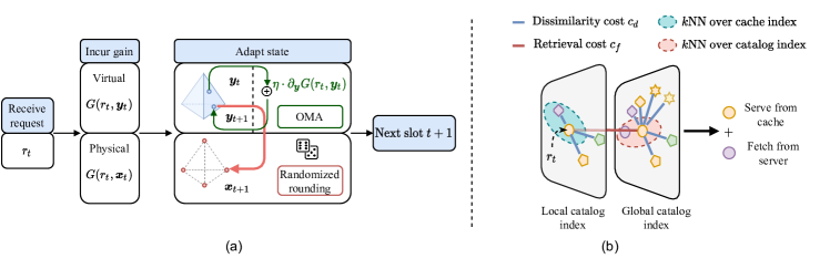
Figure 1: Subfigure (a) illustrates AÇAI’s state adaptation. A time slot is initiated when a request $r_{t}$ is received. A virtual (fictitious) gain $G(r_{t},\bm{\mathbf{y}}_{t})$ and a physical gain $G(r_{t},\bm{\mathbf{x}}_{t})$ are incurred. The virtual cache adapts its fractional state by calling Online Mirror Ascent to obtain a new state $\bm{\mathbf{y}}_{t+1}\in\mathrm{conv}(\mathcal{X})$ employing the subgradient of the virtual gain $\partial_{\bm{\mathbf{y}}}G(r_{t},\bm{\mathbf{y}}_{t})$, and the new state is randomly rounded to a valid cache state $\bm{\mathbf{x}}_{t+1}\in\mathcal{X}$. Subfigure (b) depicts how AÇAI employs the two indexes (local catalog index and global catalog index). Approximate $k$NN queries are performed on each index, and the contents with the least overall costs are selected.

IV-A Cost Assumptions

Many of the similarity caching policies proposed in the literature (including SIM-LRU, CLS-LRU, RND-LRU, and QCache) have not been designed with a clear quantitative objective, but with the qualitative goal of significantly reducing the fetching cost without increasing too much the dissimilarity cost. Because of such vagueness, the corresponding papers do not make clear assumptions about the dissimilarity costs and the fetching costs. On the contrary, AÇAI has been designed to minimize the total cost of the similarity search system and we make explicit the corresponding hypotheses.

TABLE I: Notation Summary

	Notational Conventions
$\mathbbm{1}_{\chi}$	Indicator function set to 1 when condition $\chi$ is true
$[n]$	Set of integers $\{1,2,\dots,n\}$
$\mathrm{conv}(S)$	Convex hull of a set $S$
	System Model
$\mathcal{N}$	Catalog of $N$ objects
$\mathcal{U}$	Augmented catalog of $2N$ objects
$x_{i}$	0-1 indicator variable set to 1 when $i\in\mathcal{N}$ is cached, and $x_{i}=1-x_{i-N}$ for $i\in\mathcal{U}\setminus\mathcal{N}$
$h$	Cache capacity
$r\,/\,\mathcal{R}$	Request / Request set
$c_{f}$	Retrieval cost
$c_{d}(r,o)$	Dissimilarity cost of serving object $o$ to request $r$
$c(r,o)$	Overall cost of serving object $o$ to request $r$
$\pi^{r}$	Permutation of the elements of $\mathcal{U}$, where $\pi^{r}_{i}$ gives the $i$-th closest object to $r$
$\alpha^{r}_{i}$	Cost difference between the $(i+1)$-th smallest cost and the $i$-th smallest cost when serving request $r$
$K^{r}$	The order of the largest possible cost when $r$ is requested.
$k\mathrm{NN}(r,S)$	Set of $k$ closest objects to $r$ in $S\subset\mathcal{N}$ according to $c(r,\,\cdot\,)$
$\bm{\mathbf{x}}\,/\,\mathcal{X}$	Cache state vector / Set of valid cache states
$t\,/\,T$	Time slot / Time horizon
$C(r,\bm{\mathbf{x}})$	Total cost to serve request $r$ under cache allocation $\bm{\mathbf{x}}$
$G(r,\bm{\mathbf{x}})$	Total caching gain to serve request $r$ under cache allocation $\bm{\mathbf{x}}$
$\mathcal{C}_{\text{UC},T}$	Update cost of the system over time horizon $T$
$G_{T}(\bm{\mathbf{x}})$	Time-averaged caching gain
	AÇAI
$\Phi$	Mirror map
$\mathcal{D}$	Domain of the mirror map
$\bm{\mathbf{y}}$	Fractional cache state
$\eta$	Learning rate
$\bm{\mathbf{g}}_{t}$	Subgradient of $G(r_{t},\bm{\mathbf{y}})$ at point $\bm{\mathbf{y}}_{t}$
$\prod_{S}^{\Phi}(\,\cdot\,)$	Negative entropy Bregman projection onto the set $S$
$M$	Freezing period
$c_{d}^{k}$	Upper bound on the dissimilarity cost of the k-th closest object for any request
$\psi$	Static optimum discount factor

Our main assumption is that all costs are additive. The function $c_{d}(r,o)$ introduced in Sec. II quantifies the dissimilarity of the object $o$ and the request $r$. Let $\mathcal{A}$ be the set of objects in the answer to request $r$. It is natural to consider as dissimilarity cost of the answer $\sum_{o\in\mathcal{A}}c_{d}(r,o)$.

In addition, if fetching a single object from the server incurs a cost $c_{f}\in\mathbb{R}_{>0}$, the fetching cost to retrieve $m$ objects is $m\times c_{f}$. This is an obvious choice when $c_{f}$ captures server or network cost. When $c_{f}$ captures the delay experienced by the user, then summing the costs is equivalent to consider the round trip time negligible in comparison to the transmission time, which is justified for large multimedia objects. It is easy to modify AÇAI to consider the alternative case when the fetching cost does not depend on how many objects are retrieved. Finally, as common in other works [18, 25], we assume that both the dissimilarity cost and the fetching cost can be directly compared (e.g., they can both be converted into dollars). Under these assumptions, when, for example, the $k$ nearest neighbors in $\mathcal{N}$ to the query $r$ ($k\mathrm{NN}(r,\mathcal{N})$) are retrieved from the remote server, the total cost experienced by the system is $\sum_{o\in k\mathrm{NN}(r,\mathcal{N})}c_{d}(r,o)+kc_{f}$.

IV-B Cache Indexes

AÇAI departs from the key-value indexes of most of the similarity caching policies. As discussed in Sec. II, such an approach was essentially motivated by the need to simplify $k$NN searches by performing two searches on smaller datasets (the set of keys first, and then the union of the values for $l$ keys), and may lead to potential inefficiencies including sub-utilization of the available caching space.

The two-level search implemented by existing similarity caching policies can be seen as a naïve way to implement an approximate $k$NN search on the set of objects stored locally (the local catalog $\mathcal{C}$). Thanks to the recent advances in approximate $k$NN searches (Sec. III), we have now better approaches to search through large catalogs with limited memory and computation requirements. We assume then that the cache maintains two indexes supporting $k$NN searches: one for the local catalog (the objects stored locally) and one for the remote catalog (the objects stored at the server). A discussion about which approximate index is more appropriate for each catalog is in Sec. III.

The local catalog index allows AÇAI to (i) fully exploit the available space (the cache stores at any time $h$ objects and can perform a $k$NN search on all of them), (ii) potentially find closer objects in comparison to the non-optimized key-value search. Instead, the remote catalog index allows AÇAI to evaluate what objects the server would provide as an answer to the request, and then to correctly evaluate which objects should be served locally and which one should be served from the server/ as we are going to describe next.

IV-C Request Serving

Differently from existing policies, AÇAI has the possibility to compose the answer using both local objects and remote ones. Upon a request $r$, AÇAI uses the two indexes to find the closest objects from the local catalog $\mathcal{C}$ and the remote catalog $\mathcal{N}$. We denote the set of objects identified by these indexes as $k\mathrm{NN}(r,\mathcal{C})$ and $k\mathrm{NN}(r,\mathcal{N})$, respectively. AÇAI composes the answer $\mathcal{A}$ by combining the objects with the smallest costs in the two sets. For an object $o$ stored locally ($o\in\mathcal{C}$), the system only pays $c_{d}(r,o)$; for an object $o$ fetched from the remote server ($o\in\mathcal{N}\setminus\mathcal{C}$), the system pays $c_{d}(r,o)+c_{f}$. The total cost experienced is

$$C(r,\mathcal{A}) \triangleq\sum_{o\in\mathcal{A}\cap k\mathrm{NN}(r,\mathcal{C})}c_{d}(r,o)+\sum_{o\in\mathcal{A}\setminus k\mathrm{NN}(r,\mathcal{C})}\left(c_{d}(r,o)+c_{f}\right).$$ (1)

The answer $\mathcal{A}$ is determined by selecting $k$ objects that minimize the total cost, that is

$$\mathcal{A}=\operatorname*{arg\,min}_{\begin{subarray}{c}{\mathcal{B}\subset\left(k\mathrm{NN}(r,\mathcal{C})\cup k\mathrm{NN}(r,\mathcal{N})\right)}\\ {|\mathcal{B}|=k}\end{subarray}}C(r,\mathcal{B}).$$ (2)

IV-D Cache State and Service Cost/Gain

In order to succinctly present how AÇAI updates the local catalog and its theoretical guarantee, it is convenient to express the cost in (1) as a function of the current cache state and replace the set notation with a vectorial one.

First, we define the augmented catalog $\mathcal{U}\triangleq\mathcal{N}\cup\{N+1,N+2,\dots,2N\}$ and define the new costs

$$c(r,i)=\begin{cases}c_{d}(r,i),&\text{if }i\in\mathcal{N},\\ c_{d}(r,i-N)+c_{f},&\text{if }i\in\mathcal{U}\setminus\mathcal{N}.\end{cases}$$ (3)

Essentially, $i$ and $i+N$ (for $i\in\{1,\dots,N\}$) correspond to the same object, with $i$ capturing the cost when the object is stored at the cache and $i+N$ capturing the cost when it is stored at the server. From now on, when we talk about the closest objects to a request, we are considering $c(\cdot,\cdot)$ as the distance.

Note that AÇAI can easily be modified to account for heterogeneous retrieval costs by modifying Eq. (3) and replacing $c_{f}$ by an object-dependent retrieval cost $c_{f,i}$ for every object $i\in\mathcal{N}$. Moreover, we assume that the fetching cost and dissimilarity cost are added together linearly in the objective, however our model can capture the scenario where the cost is not necessarily additive in $c_{d}$ and $c_{f}$ by a redefinition of the second line in Eq. (3). In particular, the algorithm only requires the existence of an arbitrary function $c(r,i)$ and the theoretical guarantees in Sec. IV-H also hold under such modifications. We consider a simplified model to streamline the presentation.

It is also convenient to represent the state of the cache (the set of objects stored locally) as a vector $\bm{\mathbf{x}}\in\{0,1\}^{2N}$, where, for $i\in\mathcal{N}$, $x_{i}=1$ (resp., $x_{i}=0$), if $i$ is stored (resp., is not stored) in the cache, and we set $x_{i+N}=1-x_{i}$. The set of valid cache configurations is given by:

$$\mathcal{X}\triangleq\left\{\bm{\mathbf{x}}\in\{0,1\}^{2N}:\sum_{i\in\mathcal{N}}x_{i}=h,\,x_{j+N}=1-x_{j},\forall j\in\mathcal{N}\right\}.$$ (4)

For every request $r\in\mathcal{R}$ we define the sequence $\pi^{r}$ as the permutation of the elements of $\mathcal{U}$, where $\pi^{r}_{i}$ is the $i$-th closest object to $r$ in $\mathcal{U}$ according to the costs $c(r,o),\forall o\in\mathcal{U}$. The answer $\mathcal{A}$ provided by AÇAI (Eq. (2)) coincides with the first $k$ elements of $\pi^{r}$ for which the corresponding index in $\bm{\mathbf{x}}$ is equal to $1$. The total cost to serve $r$ can then be expressed directly as a function of the cache state $\bm{\mathbf{x}}$:

$$C(r,\bm{\mathbf{x}}) =\sum^{2N}_{i=1}c(r,\pi^{r}_{i})x_{\pi^{r}_{i}}\mathbbm{1}_{\left\{\sum^{i-1}_{j=1}x_{\pi^{r}_{j}}<k\right\}},\forall\bm{\mathbf{x}}\in\mathcal{X},$$ (5)

where $\mathbbm{1}_{\{\chi\}}=1$ when the condition $\chi$ is true, and $\mathbbm{1}_{\{\chi\}}=0$ otherwise.

Instead of working with the cost $C(r,\bm{\mathbf{x}})$, we can equivalently consider the caching gain defined as the cost reduction due to the presence of the cache (as in [41, 35, 42]):

$$G(r,\bm{\mathbf{x}})\triangleq C(r,(\underbrace{0,0,\dots,0}_{N},\underbrace{1,1,\dots,1}_{N}))-C(r,\bm{\mathbf{x}}),$$ (6)

where the first term corresponds to the cost when the cache is empty (and then requests are entirely satisfied by the server). The theoretical guarantees of AÇAI are simpler to express in terms of the caching gain (Sec. IV-H). Observe that the caching gain is zero for any cache state when the retrieval cost is null ($c_{f}=0$), e.g., the cache and the server are co-located. In this case, the cache would not provide any advantage.

The caching gain has the following compact expression (Supplementary material, Sec. I, Lemma 3):

$$G(r,\bm{\mathbf{x}})=\sum^{K^{r}-1}_{i=1}\alpha^{r}_{i}\min\left\{k-\sigma^{r}_{i},\sum^{i}_{j=1}x_{\pi^{r}_{j}}-\sigma^{r}_{i}\right\},$$ (7)

where

$$\sigma^{r}_{i}\triangleq\sum^{i}_{j=1}\mathbbm{1}_{\left\{\pi^{r}_{j}\in\mathcal{U}\setminus\mathcal{N}\right\}}, \forall(i,r)\in\mathcal{U}\times\mathcal{R},$$ (8)

$K^{r}$ is the value of the minimum index $i\in\mathcal{U}$ such that $\sigma^{r}_{i}=k$, and $\alpha_{i}^{r}\triangleq c(r,\pi^{r}_{i+1})-c(r,\pi^{r}_{i})\geq 0$.

Let $\mathrm{conv}(\mathcal{X})$ denote the convex hull of the set of valid cache configurations $\mathcal{X}$. We observe that $G(r,\bm{\mathbf{y}})$ is a concave function of variable $\bm{\mathbf{y}}\in\mathrm{conv}(\mathcal{X})$. Indeed, from Eq. (7), $G(r,\bm{\mathbf{y}})$ is a linear combination, with positive coefficients, of concave functions (the minimum of affine functions in $\bm{\mathbf{y}}$).

IV-E Cache Updates

We denote by $r_{t}\in\mathcal{R}$ the $t$-th request. The cache is allowed to change its state $\bm{\mathbf{x}}_{t}\in\mathcal{X}$ to $\bm{\mathbf{x}}_{t+1}\in\mathcal{X}$ in a reactive manner, after receiving the request $r_{t}$ and incurring the gain $G({r_{t}},\bm{\mathbf{x}}_{t})$. AÇAI updates its state $\bm{\mathbf{x}}_{t}$ to greedily maximize the gain.

Input: $\eta\in\mathbb{R}_{+}$, RoundingScheme

1:procedure OnlineMirrorAscent

2:    $\bm{\mathbf{y}}_{1}\leftarrow\underset{\bm{\mathbf{y}}\in\mathrm{conv}(\mathcal{X})\cap\mathcal{D}}{\arg\min}\,\Phi(\bm{\mathbf{y}});\bm{\mathbf{x}}_{1}\leftarrow\textsc{DepRound}(\bm{\mathbf{y}}_{1})$

3:    for $t\leftarrow 1,2,\dots,T$ do$\triangleright$ Incur a gain $G({r_{t}},\bm{\mathbf{y}}_{t})$, and compute a subgradient $\bm{\mathbf{g}}_{t}$ of $G$ at point $\bm{\mathbf{y}}_{t}$ (Supplementary material, Sec. V, Eq. (52))

4:        $\hat{\bm{\mathbf{y}}}_{t}\leftarrow\nabla\Phi(\bm{\mathbf{y}}_{t})$$\triangleright$ Map primal point to dual point

5:        $\hat{\bm{\mathbf{z}}}_{t+1}\leftarrow\hat{\bm{\mathbf{y}}}_{t}+\eta\bm{\mathbf{g}}_{t}$$\triangleright$ Take gradient step in the dual

6:        $\bm{\mathbf{z}}_{t+1}\leftarrow\left(\nabla\Phi\right)^{-1}(\hat{\bm{\mathbf{z}}}_{t+1})$$\triangleright$ Map dual point to a primal point

7:        $\bm{\mathbf{y}}_{t+1}\leftarrow\prod_{\mathrm{conv}(\mathcal{X})\cap\mathcal{D}}^{\Phi}(\bm{\mathbf{z}}_{t+1})$$\triangleright$ Proj. new point onto feasible region

8:$\triangleright$  Select a rounding scheme

9:        if RoundingScheme = DepRound then

10:           if  $M\,|\,t$ then $\triangleright$ Round the fractional state every $M$ requests

11:               $\bm{\mathbf{x}}_{t+1}\leftarrow\textsc{DepRound}(\bm{\mathbf{y}}_{t+1})$

12:           end if

13:        else if RoundingScheme = CoupledRounding then

14:           $\bm{\mathbf{x}}_{t+1}\leftarrow\textsc{CoupledRounding}(\bm{\mathbf{x}}_{t},\bm{\mathbf{y}}_{t},\bm{\mathbf{y}}_{t+1})$

15:        end if

16:    end for

17:end procedure

Algorithm 1 Online Mirror Ascent ($\mathrm{OMA}$)

The update of the state $\bm{\mathbf{x}}_{t}$ is driven from a continuous fractional state $\bm{\mathbf{y}}_{t}\in\mathrm{conv}(\mathcal{X})$, where $y_{t,i}$ can be interpreted as the probability to store object $i$ in the cache. At each request $r_{t}$, AÇAI increases the components of $\bm{\mathbf{y}}_{t}$ corresponding to the objects that are used to answer to $r_{t}$, and decreases the other components. This could be achieved by a classic gradient method, e.g., $\bm{\mathbf{y}}_{t+1}=\bm{\mathbf{y}}_{t}+\eta\mathbf{g}_{t}$, where $\mathbf{g}_{t}$ is a subgradient of $G(r_{t},\bm{\mathbf{y}}_{t})$ and $\eta\in\mathbb{R}_{+}$ is the learning rate (or stepsize), but in AÇAI we consider a more general online mirror ascent update $\mathrm{OMA}$ [43, Ch. 4] that is described in Algorithm 1. $\mathrm{OMA}$ is parameterized by the function $\Phi(\,\cdot\,)$, that is called the mirror map (see Supplementary material, Sec. VI). If the mirror map is the squared Euclidean norm, $\mathrm{OMA}$ coincides with the usual gradient ascent method, but other mirror maps can be selected. In particular, our experiments in Sec. V show that the negative entropy map $\Phi(\bm{\mathbf{y}})=\sum_{i\in\mathcal{N}}y_{i}\log y_{i}$ with domain $\mathcal{D}=\mathbb{R}^{N}_{>0}$ achieves better performance.

IV-F Rounding the Cache Auxiliary State

At every time slot $t\in[T]$, AÇAI can use the randomized rounding scheme DepRound[44] to generate a cache allocation $\bm{\mathbf{x}}_{t+1}\in\mathcal{X}$ from $\bm{\mathbf{y}}_{t+1}\in\mathrm{conv}(\mathcal{X})$, while still satisfying the capacity constraint at any time slot $t$. The cache can fetch from the server the objects that are in $\bm{\mathbf{x}}_{t+1}$ but not in $\bm{\mathbf{x}}_{t}$.

As cache updates introduce extra costs for the network operator, DepRound could potentially cause extra update costs that grow linearly in time. To mitigate incurring large update costs, we may avoid updating the cache state at every time slot $t\in[T]$ by freezing the cache physical state for $M\in[T]$ time steps. In particular, we assume the update cost of the system to be proportional to the number of fetched files, which can be upper bounded by the $l_{1}$ norm of the state update: $\sum_{i\in\mathcal{N}}\max\{0,x_{t+1,i}-x_{t,i}\}\leq\left\lVert\bm{\mathbf{x}}_{t+1}-\bm{\mathbf{x}}_{t}\right\rVert_{1}$. Hence, if we denote by $\mathcal{C}_{\mathrm{UC},T}$ the total update cost of the system over the time horizon $T$, then we have

$$\mathcal{C}_{\mathrm{UC},T}=\mathcal{O}\left(\sum^{T-1}_{t=1}\left\lVert\bm{\mathbf{x}}_{t+1}-\bm{\mathbf{x}}_{t}\right\rVert_{1}\right).$$ (9)

When the cache state is refreshed after a call to the rounding scheme DepRound, the incurred update cost is in the order of $\operatorname{\mathcal{O}}\left(2h\right)$, and $\frac{\mathcal{C}_{\mathrm{UC},T}}{T}=\operatorname{\mathcal{O}}\left(\frac{2h}{M}\right)$. Moreover, when $M=\Theta\left(T^{\beta}\right)$ for $\beta\in(0,1)$ it holds $\frac{\mathcal{C}_{\mathrm{UC},T}}{T}=\operatorname{\mathcal{O}}\left(T^{-\beta}\right),$ and for any $\epsilon>0$ and $T$ large enough

$$\frac{\mathcal{C}_{\mathrm{UC},T}}{T}\leq\epsilon.$$ (10)

The average update cost of the system is then negligible for large $T$. The parameter $M$ reduces cache updates at the expense of reducing the cache reactivity (see Theorem IV.3).

In some applications, it is possible to slightly violate the capacity constraint with small deviations, as long as this is satisfied on average [45, 46, 47]. For example, there could be a monetary value associated to the storage reserved by the cache, and a total budget available over a target time horizon $T$. In this setting, the cache may violate momentarily the capacity constraint, as far as the total payment does not exceed the budget.

CoupledRounding (Algorithm 2) is a rounding approach which works under this relaxed capacity constraint and does not require freezing the cache state for $M$ time slots. At time slot $t\in[T]$, the cache decides which files to cache through $N$ coin tosses, where the file $i\in\mathcal{N}$ is cached with probability $y_{t,i}$, and the random state obtained is $\bm{\mathbf{x}}_{t}$. By definition, the expected value of the integral state is $\mathbb{E}[\bm{\mathbf{x}}_{t}]=\bm{\mathbf{y}}_{t}$. The probability that the cache exceeds its target storage capacity by $\delta h$ is given by the Chernoff bound [48] as:

$$\mathbb{P}\left(\left\lVert\bm{\mathbf{x}}_{t}\right\rVert_{1}>(1+\delta)h\right)<e^{\frac{-\delta^{2}h}{2}},\delta\in(0,1],$$ (11)

where the $l_{1}$ norm is restricted to the first $N$ components of the vector, i.e., $\left\lVert\bm{\mathbf{x}}\right\rVert_{1}\triangleq\sum_{i\in\mathcal{N}}|x_{i}|$. In the regime of large cache sizes $h\gg 1$, we observe from the Chernoff bound that the cache stores less than $(1+\delta)$ of its target capacity $h$ with high probability.

Theorem IV.1 (proof in Supplementary material, Sec. VIII-A) shows that the expected movement of CoupledRounding is equal to the movement of the fractional auxiliary states $\{\bm{\mathbf{y}}_{t}\}^{T}_{t=1}$.

Theorem IV.1.

If the input to Algorithm 2 is sampled from a random variable $\bm{\mathbf{x}}_{t}\in\{0,1\}^{N}$ with $\mathbb{E}[\bm{\mathbf{x}}_{t}]=\bm{\mathbf{y}}_{t}$, then we obtain as output an integral cache configuration $\bm{\mathbf{x}}_{t+1}\in\{0,1\}^{N}$ satisfying $\mathbb{E}[\bm{\mathbf{x}}_{t+1}]=\bm{\mathbf{y}}_{t+1}$ and $\mathbb{E}\left[\left\lVert\bm{\mathbf{x}}_{t+1}-\bm{\mathbf{x}}_{t}\right\rVert_{1}\right]={\left\lVert\bm{\mathbf{y}}_{t+1}-\bm{\mathbf{y}}_{t}\right\rVert_{1}}$.

Moreover, the movement of the fractional states is negligible for large $T$:

Theorem IV.2.

Algorithm 1, configured with the negative entropy mirror map and learning rate $\eta=\operatorname{\mathcal{O}}\left(\frac{1}{\sqrt{T}}\right)$, selects fractional cache states satisfying

$$\sum^{T-1}_{t=1}\left\lVert\bm{\mathbf{y}}_{t+1}-\bm{\mathbf{y}}_{t}\right\rVert_{1}=\mathcal{O}(\sqrt{T}).$$ (12)

The proof is in Supplementary material, Sec. VIII-B.

Combining the two theorems and (9), we also conclude that the expected average update cost of the system $\mathbb{E}\left[\frac{\mathcal{C}_{\mathrm{UC},T}}{T}\right]$ is negligible for large $T$.

Input: $\bm{\mathbf{x}}_{t},\bm{\mathbf{y}}_{t},\bm{\mathbf{y}}_{t+1}$ $\triangleright$ $\bm{\mathbf{x}}_{t}$ satisfies $\mathbb{E}[\bm{\mathbf{x}}_{t}]=\bm{\mathbf{y}}_{t}$

1:procedure CoupledRounding

2:    $\delta\leftarrow\bm{\mathbf{y}}_{t+1}-\bm{\mathbf{y}}_{t}$ $\triangleright$ Compute the change in distribution

3:    for $i\in\mathcal{N}$ do

4:        if $\left(x_{t,i}=1\right)\land\left(\delta_{i}<0\right)$ then

5:           $x_{t+1,i}\leftarrow 0$ w.p. $-\frac{\delta_{i}}{y_{t,i}}$, and $x_{t+1,i}\leftarrow 1$ w.p. $\frac{y_{t,i}+\delta_{i}}{y_{t,i}}$

6:        else if $\left(x_{t,i}=0\right)\land\left(\delta_{i}>0\right)$ then

7:           $x_{t+1,i}\leftarrow 0$ w.p. $\frac{1-y_{t,i}-\delta_{i}}{1-y_{t,i}}$, and $x_{t+1,i}\leftarrow 1$ w.p. $\frac{\delta_{i}}{1-y_{t,i}}$

8:        else

9:           $x_{t+1,i}\leftarrow x_{t,i}$ $\triangleright$ Keep the same state

10:        end if

11:        $x_{t+1,i+N}\leftarrow 1-x_{t+1,i}$ $\triangleright$ Update the augmented states

12:    end for

13:    return $\bm{\mathbf{x}}_{t+1}$ $\triangleright$ Return the next physical state satisfying $\mathbb{E}[\bm{\mathbf{x}}_{t+1}]=\bm{\mathbf{y}}_{t+1}$

14:end procedure

Algorithm 2 Coupled Rounding

IV-G Time Complexity

AÇAI uses $\mathrm{OMA}$ in Algorithm 1 coupled with a rounding procedure DepRound or CoupledRounding. The rounding step may take $\operatorname{\mathcal{O}}\left(N\right)$ operations (amortized every $M$ requests when DepRound is used). In practice, AÇAI quickly sets irrelevant objects in the fractional allocation vector $\bm{\mathbf{y}}_{t}$ very close to 0. Therefore, we can keep track only of objects with a fractional value above a threshold $\epsilon>0$, and the size of this subset is practically of the order of $h$.

Similarly, subgradient computation (see Supplementary material, Sec. V, Eq. (52)) may require $\operatorname{\mathcal{O}}\left(N\right)$ operations per each component and then have $\operatorname{\mathcal{O}}\left(N^{2}\right)$ complexity, but in practice, as the vector $\bm{\mathbf{y}}_{t}$ is sparse, calculations require only a constant number of operations and complexity reduces to $\operatorname{\mathcal{O}}\left(N\right)$.

Finally, we use the negative entropy Bregman projection in [38] (line 6 of Algorithm 1) that has $\operatorname{\mathcal{O}}\left(N+h\log(h)\right)$ time complexity. The $\operatorname{\mathcal{O}}\left(N+h\log(h)\right)$ is due to a partial sorting operation while the actual projection takes $\operatorname{\mathcal{O}}\left(h\right)$. Again, most of the components of $\bm{\mathbf{y}}_{t}$ are equal to $0$, so that, in practice, we need to sort much fewer points.

IV-H Theoretical Guarantees

The best static cache allocation in hindsight is the cache state $\bm{\mathbf{x}}_{*}$ that maximizes the time-averaged caching gain in Eq. (6) over the time horizon $T$, i.e.,

$$\bm{\mathbf{x}}_{*}\in\underset{\bm{\mathbf{x}}\in\mathcal{X}}{\operatorname*{arg\,max}}\left(G_{T}(\bm{\mathbf{x}})\triangleq\frac{1}{T}\sum^{T}_{t=1}G(r_{t},\bm{\mathbf{x}})\right).$$ (13)

We observe that solving (13) is NP-hard in general even for $k=1$ under a stationary request process [18]. Nevertheless, AÇAI operates in the online setting and provides guarantees in terms of the $\psi$-regret [49]. In this scenario, the regret is defined as a gain loss in comparison to the best static cache allocation $\bm{\mathbf{x}}_{*}$ in (13). The $\psi$-regret discounts the best static gain by a factor $\psi\in(0,1]$. Formally,

$$\text{$\psi$-}{\mathrm{Regret}_{T,\mathcal{X}}}(\mathrm{OMA}_{\Phi})=$$

$$\underset{\{r_{1},r_{2},\dots,r_{T}\}\in\mathcal{R}^{T}}{\sup}\left\{\psi\sum^{T}_{t=1}G({r}_{t},\bm{\mathbf{x}}_{*})-\mathbb{E}\left[\sum^{T}_{t=1}G({r}_{t},\bm{\mathbf{x}}_{t})\right]\right\},$$ (14)

where the expectation is over the randomized choices of DepRound. Note that the supremum in (14) is over all possible request sequences. This definition corresponds to the so-called adversarial analysis, imagining that an adversary selects requests in $\mathcal{R}$ to jeopardize cache performance. The definition of the regret in Eq. (14), which compares the gain of the policy to a static offline solution, is classic. Several bandit settings, e.g., simple multi-armed bandits [50, 51, 52], contextual bandits [53, 54, 55], and, of course, their applications to caching problems under the full-information setting [28, 38, 40, 56, 57], adopt this definition. In all these cases, the dynamic, adaptive algorithm is compared to a static policy that has full hindsight of the entire trace of actions. Moreover, as is customary when the offline problem is NP-hard [58], the regret is not w.r.t. the optimal caching gain, but w.r.t. the gain obtained by an offline approximation algorithm. Regret bounds in the adversarial setting provide strong robustness guarantees in practical scenarios. AÇAI has the following regret guarantee:

Theorem IV.3.

Algorithm 1 configured with the negative entropy mirror map, learning rate $\eta=\frac{1}{(c_{d}^{k}+c_{f})}\sqrt{\frac{2\log\left(\frac{N}{h}\right)}{T+(M-1)(M+T)}}$, and rounding scheme CoupledRounding or DepRound with a freezing period $M=\Theta\left({T^{\beta}}\right)$ for $\beta\in[0,1)$, has a sublinear $(1-1/e)$-regret in the number of requests, i.e.,

$$\text{$\left(1-1/e\right)$-}{\mathrm{Regret}_{T,\mathcal{X}}}(\mathrm{OMA}_{\Phi})$$

$$\leq\left(1-\frac{1}{e}\right)(c_{d}^{k}+c_{f})h\sqrt{2\log{\left(\frac{N}{h}\right)}((M-1)(T+M)+T)},$$

where the constant $c_{d}^{k}$ is an upper bound on the dissimilarity cost of the k-th closest object for any request in $\mathcal{R}$.

Proof.

(sketch) We first prove that the expected gain of the randomly sampled allocations $\bm{\mathbf{x}}_{t}$ is a $(1{-}1/e)$-approximation of the fractional gain. Then, we use online learning results [43] to bound the regret of OMA schemes operating on a convex decision space against concave gain functions picked by an adversary. The two results are combined to obtain an upper bound on the $(1{-}1/e)$-regret. The full proof is available in Supplementary material, Sec. IX. ∎

The $(1-1/e)$-regret of AÇAI under CoupledRounding scheme has order-optimal regret $\operatorname{\mathcal{O}}\left(\sqrt{T}\right)$ [59]. Under the rounding scheme DepRound with freezing period $M=\Theta\left({T^{\beta}}\right)$, the reduced reactivity of AÇAI is reflected by the additional $T^{\frac{\beta}{2}}$ factor in the order of the regret. Nonetheless, the expected time-average $(1-1/e)$-regret of AÇAI can get arbitrarily close to zero for a large time horizon. Hence, AÇAI performs on average as well as a $(1-1/e)$-approximation of the optimal configuration $\bm{\mathbf{x}}_{*}$. This observation also suggests that our algorithm can be used as an iterative method to solve the NP-hard static allocation problem with the best approximation bound achievable for these kinds of problems [60].

Corollary IV.3.1.

(offline solution) Let $\bar{\bm{\mathbf{y}}}$ be the average fractional allocation $\bar{\bm{\mathbf{y}}}=\frac{1}{\tilde{T}}\sum^{\tilde{T}}_{i=1}\bm{\mathbf{y}}_{i}$ of AÇAI, and $\bar{\bm{\mathbf{x}}}$ the random state sampled from $\bar{\bm{\mathbf{y}}}$ through CoupledRounding or DepRound. If Algorithm 1 is configured with the negative entropy mirror map, and, at each iteration $t\in[\tilde{T}]$, operates with subgradients of the time-averaged caching gain (13), then $\forall\epsilon>0$ and over a sufficiently large number of iterations $\tilde{T}$, $\bar{\bm{\mathbf{x}}}$ satisfies

$$\mathbb{E}\left[G_{T}(\bar{\bm{\mathbf{x}}})\right]\geq\left(1-\frac{1}{e}-\epsilon\right)G_{T}({\bm{\mathbf{x}}_{*}}).$$

where $\bm{\mathbf{x}}_{*}=\underset{\bm{\mathbf{x}}\in\mathcal{X}}{\arg\max}~{}G_{T}(\bar{\bm{\mathbf{x}}})$.

The proof can be found in Supplementary material, Sec. X.

V Experiments

We start evaluating AÇAI in a simple scenario with a synthetic request process, for which we can compute the optimal fractional static cache allocation. We then consider real-world catalogs and traces and compare our solution with state-of-the-art online policies proposed for $k$NN caching, i.e., SIM-LRU [17], CLS-LRU [17], and QCache [27] described in Sec. II.

V-A Simple Scenario

As in [61], we consider a synthetic catalog of $N=900$ objects positioned on a $30\times 30$ grid. The request process is generated according to the Independent Reference Model [62]. The objects’ popularity is represented by a Gaussian distribution. In particular, an object $o\in\mathcal{N}$ with $l_{1}$ distance $d_{o}$ from the center of the grid (15, 15) is requested at any time slot $t$ with probability $p_{o}\propto e^{-\frac{d^{2}_{o}}{2\times 6^{2}}}$. The synthetic catalog is depicted in Fig. 2.

We consider the dissimilarity cost to be the $l_{1}$ distance. We take different values for the retrieval cost $c_{f}\in\{1,2,3,4\}$ and the number of neighbors $k\in\{1,2,3,4,5\}$. We take the cache capacity to be $h=15$. We configure AÇAI with DepRound rounding scheme.

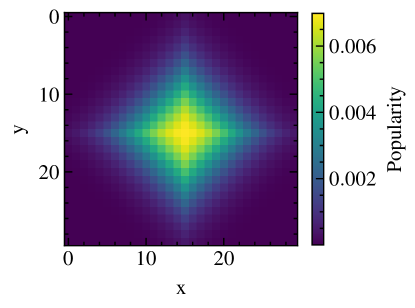
Figure 2: Synthetic catalog of objects located on a $30\times 30$ grid. The heatmap depicts the popularity distribution of objects in the grid.

We use CVXPY [63] to find the optimal fractional static cache allocation, and AÇAI to compute its approximation according to Corollary IV.3.1. In particular, AÇAI runs for $T=10\,000$ iterations with a diminishing learning rate $\eta_{t}=\frac{2.0}{c_{f}}(1+\cos(\frac{\pi t}{T}))$.

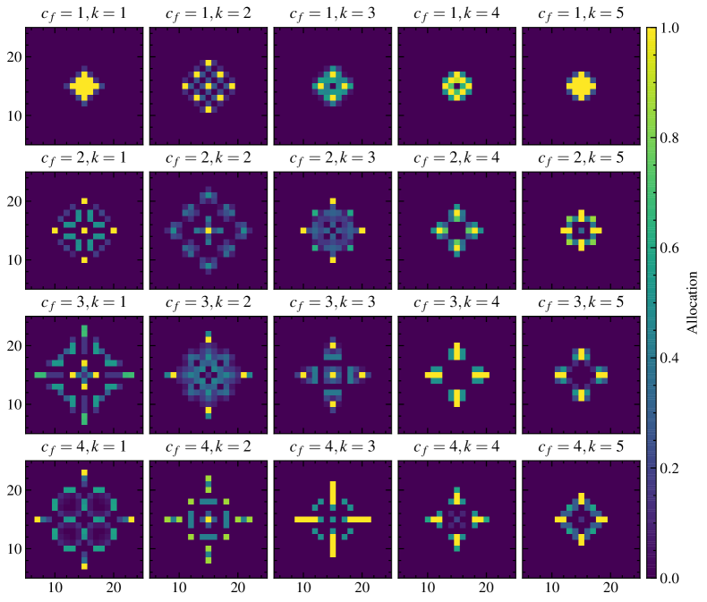
(a) Optimal fractional static cache allocations

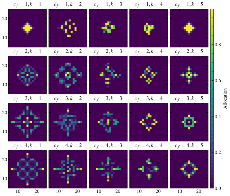
(b) AÇAI’s fractional static cache allocations

Figure 3: The optimal fractional static cache allocations, and AÇAI’s fractional static cache allocations under different values of the retrieval costs $c_{f}\in\{1,2,3,4\}$ and of the number of neighbors $k\in\{1,2,3,4,5\}$.

Results. Figure 3 shows the optimal fractional static cache allocations and the AÇAI’s fractional static cache allocations (see Corollary IV.3.1) under different retrieval costs and the number of neighbors $k$. We observe that the optimal fractional static cache allocations in Fig. 3 (a) are symmetric, while AÇAI’s fractional static cache allocations in Fig. 3 (b) partially lose this symmetry for values of $k\in\{2,3,4\}$ primarily due to the different ways a $k$NN query can be satisfied over the physical catalog for such values. In fact, there are multiple objects in the catalog with the same distance from a request $r$, and AÇAI only selects a single permutation $\pi^{r}$ for a request $r$. We observe that, when the retrieval cost is higher, the allocations are more spread to cover a larger part of the popular region.

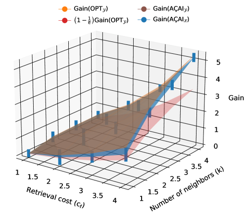
Figure 4: The gain of the optimal fractional static cache allocations ($\mathrm{Gain}(\mathrm{OPT}_{\mathcal{Y}})$), its $(1-\frac{1}{e})$-approximation, and the gain obtained by AÇAI’s fractional static cache allocations ($\mathrm{Gain}(\mathrm{A\c{C}AI}_{\mathcal{Y}})$) and static integral cache allocations ($\mathrm{Gain}(\mathrm{A\c{C}AI}_{\mathcal{X}})$) under different values of the retrieval cost $c_{f}\in\{1,2,3,4\}$ and of the number of neighbors $k\in\{1,2,3,4,5\}$. For AÇAI’s static integral cache allocations, we report 95% confidence intervals computed over 50 different runs. The gain of the fractional static cache allocations obtained by AÇAI overlaps with the gain of the optimal fractional static cache allocations.

In Fig. 4, we compare the gain obtained by the optimal fractional static cache allocations, its $(1-\frac{1}{e})$-approximation, and the gain obtained by AÇAI’s fractional static cache allocations and the static integral cache allocations (see Corollary IV.3.1). While Fig. 3 shows that AÇAI’s fractional static cache allocations may differ from the optimal ones, their costs are practically indistinguishable (the two corresponding surfaces overlap in Fig. 4). We also observe that rounding comes at a cost, as there is a clear gap between the gain of AÇAI’s fractional cache allocations and of AÇAI’s integral ones. Still, the average gain of the integral cache allocations remains close to the fractional optimum and well above the $(1-\frac{1}{e})$-approximation. AÇAI then performs much better than what is guaranteed by Corollary IV.3.1 (a potential gain reduction by a factor $1-\frac{1}{e}$).

V-B Real-world Datasets

SIFT1M trace. SIFT1M is a classic benchmark dataset to evaluate approximate $k$NN algorithms [64]. It contains 1 million objects embedded as points in a 128-dimensional space. SIFT1M does not provide a request trace so we generated a synthetic one according to the Independent Reference Model [62] (similar to what is done in other papers like [16, 23]). Request $r_{t}$ is for object $i$ with a probability $\lambda_{i}$ independently of previous requests. We spatially correlated objects’ popularities by letting $\lambda_{i}$ depend on the position of the embeddings in the space. In particular, we considered the barycenter of the whole dataset and set $\lambda_{i}$ proportional to $d_{i}^{-\beta}$, where $d_{i}$ is the distance of $i$ from the barycenter. The parameter $\beta$ was chosen such that the tail of the ranked objects’ popularity distribution is similar to a Zipf with parameter $0.9$, as observed in some image retrieval systems [27]. We generated a trace with $10^{5}$ requests. The number of distinct objects requested in the trace is approximately $2\times 10^{4}$.

Amazon trace. The authors of [65] crawled the Amazon web-store and collected a dataset to model relationships among products and provide user recommendations. They took as input the visual features of product images obtained from a machine learning model pre-trained on 1.2 million images from ImageNet. The visual features are augmented with the relationships between the items, and these relationships are collected based on the cosine similarity of the sets of users who purchased or viewed the items. The objects’ dissimilarity is modeled as a distance $d(\cdot,\cdot)$, such that $\mathbb{P}(\text{item }i\text{ is related to item }j)$ increases monotonically with $d(\bm{\mathbf{x}}_{i},\bm{\mathbf{x}}_{j})$, where $\bm{\mathbf{x}}_{i}$ and $\bm{\mathbf{x}}_{j}$ are the visual features of the items $i$ and $j$. The authors of [65] show that the relationship ‘users who viewed $i$ also viewed $j$’ can successfully be used to provide accurate recommendations. The authors of [25] built a request trace from the timestamped user reviews for objects in the category Baby embedded in a $100$-dimensional space. Two products $o$ and $o^{\prime}$ are considered similar if they have been viewed by the same users. We use the request trace from [25] and in particular the interval $[2\times 10^{5},3\times 10^{5}]$. The number of distinct objects requested in this trace is approximately $2\times 10^{4}$.

V-C Settings and Performance Metrics

For AÇAI, unless otherwise said, we choose the negative entropy $\Phi(\bm{\mathbf{y}})=\sum_{i\in\mathcal{N}}y_{i}\log(y_{i})$ as mirror map (see Fig. 10 and the corresponding discussion for other choices) and the rounding scheme DepRound with $M=1$. The learning rate is set to the best value found exploring the range $[10^{-6},10^{-4}]$.

As for the state-of-the-art caching policies, SIM-LRU and CLS-LRU have two parameters, $C_{\theta}$ and $k^{\prime}$, that we set in each experiment to the best values we found exploring the ranges $[c_{f},2c_{f}]$ for $C_{\theta}$ and $[1,h]$ for $k^{\prime}$. For QCache we consider $l=h/k$: the cache can then perform the $k$NN search over all local objects.

We also consider a simple similarity caching policy that stores previous requests and the corresponding set of $k$ closest objects as key-value pairs, and manages the set of keys according to LRU. The cache then serves locally the request if it coincides with one of the previous requests in its memory, it forwards it to the server, otherwise. The ordered list of keys is updated as in LRU. We refer to this policy simply as LRU.

We compare the policies in terms of their normalized average caching gain per request, where the normalization factor corresponds to the caching gain of a cache with a size equal to the whole catalog. In such a case, the cache could store the entire catalog locally and would achieve the same dissimilarity cost of the server without paying any fetching cost. The maximum possible caching gain is then $kc_{f}$. The normalized average gain of a policy $\mathcal{P}$ with cache states $\{\bm{\mathbf{x}}_{t}\}^{T}_{t=1}$ over $T$ requests can then be defined as:

$$\mathrm{NAG}(\mathcal{P})=\frac{1}{kc_{f}T}\sum^{T}_{t=1}G(r_{t},\bm{\mathbf{x}}_{t}).$$ (15)

V-D Results

We consider a dissimilarity cost proportional to the squared Euclidean distance. This is the usual metric considered for SIFT1M benchmark and also the one considered to learn the embeddings for the Amazon trace in [65].

The numerical value of the fetching cost depends on its interpretation (delay experienced by the user, load on the server or on the network) as well as on the application, because it needs to be converted into the same unit of the approximation cost. In our evaluation, we let it depend on the topological characteristics of the dataset in order to be able to compare the results for the two different traces. Unless otherwise said, we set $c_{f}$ equal to the average distance of the 50-th closest neighbor in the catalog $\mathcal{N}$.

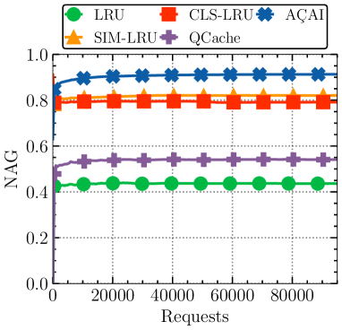
(a) SIFT1M trace

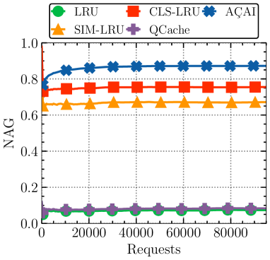
(b) Amazon trace

Figure 5: Caching gain for the different policies. The cache size is $h=1000$ and $k=10$.

Figure 5 shows how the normalized average gain changes as requests arrive and the different caching policies update the local set of objects (starting from an empty configuration). The cache size is $h=1000$ and the cache provides $k=10$ similar objects for each request. All policies reach an almost stationary gain after at most a few thousand requests. Unsurprisingly, the naïve LRU has the lowest gain (it can only satisfy locally requests that match exactly a previous request) and similarity caching policies perform better. AÇAI has a significant improvement in comparison to the second best policy (SIM-LRU for SIFT1M and CLS-LRU for Amazon).

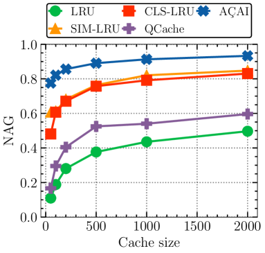
(a) SIFT1M trace

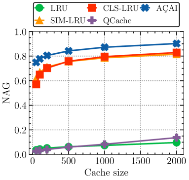
(b) Amazon trace

Figure 6: Caching gain for the different policies, for different cache sizes $h\in\{50,100,200,500,1000,2000\}$ and $k=10$.

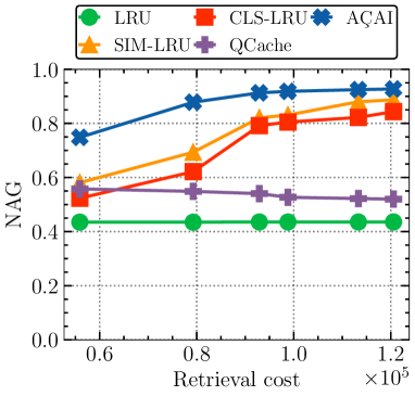
(a) SIFT1M trace

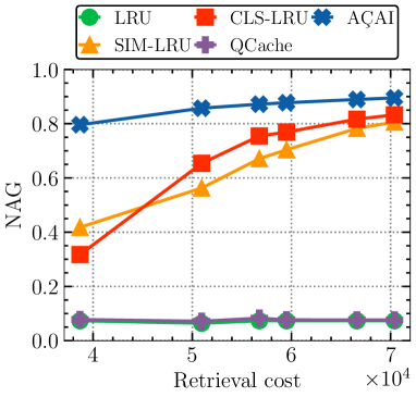
(b) Amazon trace

Figure 7: Caching gain for the different policies and different retrieval costs. The retrieval cost $c_{f}$ is taken as the average distance to the $i$-th neighbor, $i\in\{2,10,50,100,500,1000\}$. The cache size is $h=1000$ and $k=10$.

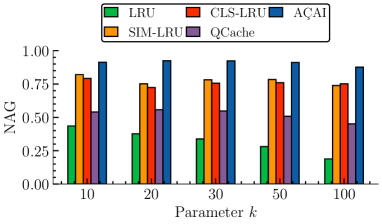
(a) SIFT1M trace

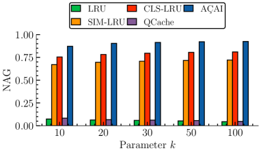
(b) Amazon trace

Figure 8: Caching gain for the different policies. The cache size is $h=1000$, and $k\in\{10,20,30,50,100\}$.

This advantage of AÇAI is constantly confirmed for different cache sizes (Fig. 6), different values of the fetching cost $c_{f}$ (Fig. 7), and different values of $k$ (Fig. 8). The relative improvement of AÇAI, in comparison to the second best policy, is larger for small values of the cache size ($+30\%$ for SIFT1M and $+25\%$ for Amazon when $h=50$), and small values of the fetching cost ($+35\%$ for SIFT1M and $+100\%$ for $c_{f}$ equal to the average distance from the second closest object). Note how these are the settings where caching choices are more difficult (and indeed all policies have lower gains): when cache storage can accommodate only a few objects, it is critical to carefully select which ones to store; when the server is close, the costs of serving requests from the cache or the server are similar and it is difficult to correctly decide how to satisfy the request. The performance of caching policies is in general less dependent on the number $k$ of similar objects to retrieve and AÇAI achieves about $10\%$ improvement for $k$ between $10$ and $100$ when $h=1000$ (Fig. 8).

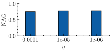
(a) AÇAI, $h=50$

(b) AÇAI, $h=10^{3}$

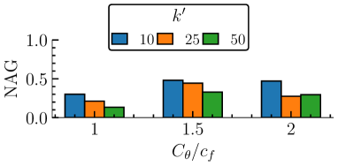
(c) SIM-LRU, $h=50$

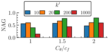
(d) SIM-LRU, $h=10^{3}$

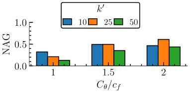
(e) CLS-LRU, $h=50$

(f) CLS-LRU, $h=10^{3}$

Figure 9: Caching gain for AÇAI for different values of $\eta$ (top). Caching gain for SIM-LRU(middle) and CLS-LRU (bottom) for different values of the parameters $(k^{\prime},C_{\theta})$. SIFT1M trace.

Sensitivity analysis. We now evaluate the robustness of AÇAI to the configuration of its single parameter (the learning rate $\eta$). Figure 9 shows indeed that, for learning rates that are two orders of magnitude apart, we can achieve almost the same normalized average gain both for $h=50$ and for $h=1000$.

In contrast, the performance of the second best policies (SIM-LRU and CLS-LRU) are more sensitive to the choice of their two configuration parameters $k^{\prime}$ and $C_{\theta}$. For example, the optimal configuration of SIM-LRU is $k^{\prime}=10$ and $C_{\theta}=1.5\times c_{f}$ for a small cache ($h=50$) but $k^{\prime}=200$ and $C_{\theta}=2\times c_{f}$ for a large one ($h=1000$). Moreover, in both cases a misconfiguration of these parameters would lead to significant performance degradation.

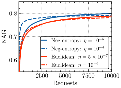
Figure 10: Caching gain for AÇAI configured with negative entropy and Euclidean maps (SIFT1M trace). The cache size is $h=100$ and $k=10$.

Choice of the mirror map. If the mirror map is selected equal to the squared Euclidean norm, the $\mathrm{OMA}$ update coincides with a standard gradient update. Figure 10 shows the superiority of the negative entropy map: it allows one to achieve a higher gain than the Euclidean norm map or the same gain but in a shorter time. To the best of our knowledge, ours is the first paper that shows the advantage of using non-Euclidean mirror maps for similarity caching problems. We observe how our finding is in apparent contrast with what observed for exact caches in [38], i.e., that the Euclidean mirror map should always be preferred when requests are not batched. The difference can be explained as follows: under exact caching only the requested object can satisfy the request and then the gradient has a single non-null component, but, under similarity caching, multiple objects in the vicinity of a request can contribute to reduce the cost of serving it and the gradient is then less sparse. It is known that denser gradients may lead to prefer the negative entropy map [43, Sec. 4.3] and our results in Supplementary material, Sec. VII-A provide a theoretical justification for our specific problem.

Dissecting AÇAI performance. In comparison to state-of-the-art similarity caching policies, AÇAI introduces two key ingredients: (i) the use of fast, approximate indexes to decide what to serve from the local catalog and what from the remote one, and (ii) the $\mathrm{OMA}$ algorithm to update the cache state. It is useful to understand how much each ingredient contributes to AÇAI improvement with respect to the other policies.

To this aim, we integrated the same indexes in the other policies allowing them to serve requests as AÇAI does, combining both local objects and remote ones based on their costs (see Sec. IV-C), while leaving their cache updating mechanism unchanged. We then compute, in the same setting of Fig. 8, how much the gain of the second best policy (SIM-LRU for SIFT1M and CLS-LRU for Amazon) increases because of AÇAI request service mechanism. This is the part of AÇAI improvement attributed to the use of the two indexes, the rest is attributed to the cache update mechanism through $\mathrm{OMA}$. We observe from Fig. 11 that most of AÇAI gain improvement over the second best caching policy is due to the use of approximate indexes, but $\mathrm{OMA}$ updates are still responsible for $15$–$20\%$ of AÇAI performance improvement under SIFT1M trace and $20$–$35\%$ for the Amazon trace.

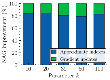
(a) SIFT1M trace

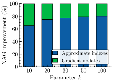
(b) Amazon trace

Figure 11: AÇAI caching gain improvement in comparison to the second best state-of-the-art similarity caching policy: contribution of approximate indexes and gradient updates. The cache size is $h=1000$, and $k\in\{10,20,30,50,100\}$.

Update cost. In this part, we evaluate the update cost of the different rounding schemes. We set the cache size $h=1000$ and $k=10$. We run AÇAI over the Amazon trace with a learning rate $\eta=10^{-5}$.

Figure 12 (a) gives the time-averaged number of files fetched and Figure 12 (b) gives the caching gain of the different rounding schemes. We observe that, by increasing the cache state freezing parameter $M$, the system fetches fewer files per iteration at the expense of losing reactivity and then incurring a smaller gain at the start. The coupled rounding scheme achieves the best performance as it fetches fewer files without losing reactivity.

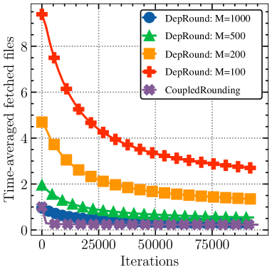
(a) Time-averaged fetched files

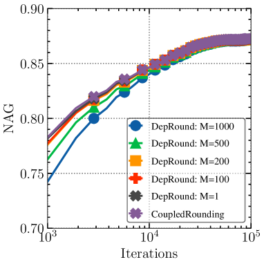
(b) Caching gain

Figure 12: Number of fetched files (time average) and caching gain of AÇAI under different rounding schemes. AÇAI is run with the learning rate $\eta=10^{-5}$ over the Amazon trace. The cache size is $h=1000$ and $k=10$.

Figure 13 shows the instantaneous and time-averaged cache occupancy of the cache using the CoupledRounding scheme with the relaxed capacity constraint. We observe that the time-averaged cache occupancy rapidly converges to the cache capacity $h$, while the instantaneous occupancy is kept within 5% of the cache capacity.

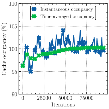
Figure 13: Time-averaged and instantaneous cache occupancy under CoupledRounding. AÇAI is run with the learning rate $\eta=10^{-5}$ over the Amazon trace. The cache size is $h=1000$ and $k=10$.

VI Conclusion

Edge computing provides computing and storage resources that may enable complex applications with tight delay guarantees like augmented-reality ones, but these strategically positioned resources need to be used efficiently. To this aim, we designed AÇAI, a content cache management policy that determines dynamically the best content to store on the edge server. Our solution adapts to the user requests, without any assumption on the traffic arrival pattern. AÇAI leverages two key components: (i) new efficient content indexing methods to keep track of both local and remote content, and (ii) mirror ascending techniques to optimally select the content to store. The results show that AÇAI is able to outperform the state-of-the-art policies and does not need careful parameter tuning.

As future work, we plan to evaluate AÇAI in the context of machine learning classification tasks [66], in which the size of the objects in the catalog is comparable to their $d$-dimensional representation in the index, and, as a consequence, the index size cannot be neglected in comparison to the local catalog size. Another important future research direction is to consider dynamic regret, whereby the performance of a policy is compared to a dynamic optimum. Also, since the employed online algorithm OMA is greedy (i.e., does not keep track of the history of the requests), with careful selection of the mirror map, it may have an adaptive regret guarantee, e.g., such guarantee holds for OGD [67].

Supplementary Material for Paper:
Ascent Similarity Caching with Approximate Indexes

I Equivalent Expression of the Cost Function

Lemma 1.

Let us fix the threshold $c\in\mathbb{N}\cup\{0\}$, $r\in\mathcal{R}$ and $i\in\mathcal{U}$. The following equality holds

$$\min\left\{c,\sum^{i}_{j=1}x_{\pi^{r}_{j}}\right\}-\min\left\{c,\sum^{i-1}_{j=1}x_{\pi^{r}_{j}}\right\}=x_{\pi_{i}^{r}}\mathds{1}_{\left\{\sum^{i-1}_{j=1}x_{\pi_{j}^{r}}<c\right\}}.$$ (16)

Proof.

We distinguish two cases:

1. When $\sum^{i-1}_{j=1}x_{\pi^{r}_{j}}\geq c$ this implies that $\sum^{i}_{j=1}x_{\pi^{r}_{j}}=x_{\pi_{j}^{r}}+\sum^{i-1}_{j=1}x_{\pi^{r}_{j}}\geq c+x_{\pi^{r}_{i}}\geq c$ since $x_{\pi^{r}_{i}}\geq 0$. Therefore, $\sum^{i-1}_{j=1}x_{\pi^{r}_{j}}\geq c$ implies that $\min\left\{c,\sum^{i-1}_{j=1}x_{\pi^{r}_{j}}\right\}=\min\left\{c,\sum^{i}_{j=1}x_{\pi^{r}_{j}}\right\}=c$, and we have:

   $$\min\left\{c,\sum^{i}_{j=1}x_{\pi^{r}_{j}}\right\}-\min\left\{c,\sum^{i-1}_{j=1}x_{\pi^{r}_{j}}\right\} =0.$$ (17)

2. When $\sum^{i-1}_{j=1}x_{\pi^{r}_{j}}<c$, we have $\sum^{i}_{j=1}x_{\pi^{r}_{j}}=x_{\pi_{j}^{r}}+\sum^{i-1}_{j=1}x_{\pi^{r}_{j}}<c+x_{\pi^{r}_{i}}\leq c$ since $x_{\pi^{r}_{i}}\leq 1$, this implies that $\min\left\{c,\sum^{i}_{j=1}x_{\pi^{r}_{j}}\right\}=\sum^{i}_{j=1}x_{\pi^{r}_{j}}$ and $\min\left\{c,\sum^{i-1}_{j=1}x_{\pi^{r}_{j}}\right\}=\sum^{i-1}_{j=1}x_{\pi^{r}_{j}}$, and we have

   $$\min\left\{c,\sum^{i}_{j=1}x_{\pi^{r}_{j}}\right\}-\min\left\{c,\sum^{i-1}_{j=1}x_{\pi^{r}_{j}}\right\} =x_{\pi^{r}_{i}}.$$ (18)

Combining Eqs. (17) and (18) yields Eq. (16). ∎

Lemma 2.

The cost function $C(r,\bm{\mathbf{x}})$ given by the expression in Eq. (5), can be equivalently expressed as:

$$C(r,\bm{\mathbf{x}}) =-\sum^{K^{r}-1}_{i=1}\alpha^{r}_{i}\min\left\{k-\sigma^{r}_{i},\sum^{i}_{j=1}x_{\pi^{r}_{j}}-\sigma^{r}_{i}\right\}+\sum^{K^{r}}_{i=1}c(r,\pi^{r}_{i})\mathds{1}_{\left\{\pi^{r}_{i}\in\mathcal{U}\setminus\mathcal{N}\right\}},$$ (19)

where $\sigma^{r}_{i}=\sum^{i}_{j=1}\mathbbm{1}_{\left\{\pi^{r}_{j}\in\mathcal{U}\setminus\mathcal{N}\right\}}$, $\alpha^{r}_{i}=c(r,\pi^{r}_{i+1})-c(r,\pi^{r}_{i})$ and $K^{r}=\min\{i\in\mathcal{U}:\sigma^{r}_{i}=k\}$ for every $(r,i)\in\mathcal{R}\times\mathcal{U}$.

Proof.

Let $\tilde{c}(r,o),\forall(r,o)\in\mathcal{R}\times\mathcal{U}$ be a cost defined as $\tilde{c}(r,{\pi^{r}_{i}})=c(r,{\pi^{r}_{i}}),\forall i\in[K^{r}]$ and 0 otherwise, and we also define $\tilde{\alpha}^{r}_{i}$ as $\tilde{\alpha}^{r}_{i}\triangleq\tilde{c}(r,{\pi^{r}_{i+1}})-\tilde{c}(r,{\pi^{r}_{i}})$.

When $i=1$ and for any $r\in\mathcal{R}$, we have

$$\tilde{c}(r,{\pi^{r}_{i}})\min\left\{k,\sum^{i-1}_{j=1}x_{\pi^{r}_{j}}\right\}=0.$$ (20)

Note that $\sigma^{r}_{1}=0$ by definition, since $\pi^{r}_{1}\in\mathcal{N}$ for any $r\in\mathcal{R}$. We have

$$-\sum^{K^{r}}_{i=1}\tilde{\alpha}^{r}_{i}\sigma^{r}_{i} =\sum^{K^{r}}_{i=1}\tilde{c}(r,{\pi^{r}_{i}})\sigma^{r}_{i}-\sum^{K^{r}}_{i=1}\tilde{c}(r,{\pi^{r}_{i+1}})\sigma^{r}_{i}=\sum^{K^{r}}_{i=1}\tilde{c}(r,{\pi^{r}_{i}})\sigma^{r}_{i}-\sum^{K^{r}}_{i=2}\tilde{c}(r,{\pi^{r}_{i}})\sigma^{r}_{i-1}$$ (21)

$$=\sum^{K^{r}}_{i=1}\tilde{c}(r,{\pi^{r}_{i}})\sigma^{r}_{i}-\sum^{K^{r}}_{i=1}\tilde{c}(r,{\pi^{r}_{i}})\sigma^{r}_{i-1}=\sum^{K^{r}}_{i=1}\tilde{c}(r,{\pi^{r}_{i}})\mathds{1}_{\left\{\pi^{r}_{i}\in\mathcal{U}\setminus\mathcal{N}\right\}}=\sum^{K^{r}}_{i=1}c(r,\pi^{r}_{i})\mathds{1}_{\left\{\pi^{r}_{i}\in\mathcal{U}\setminus\mathcal{N}\right\}}.$$ (22)

Observe that the indicator function $\mathds{1}_{\left\{\sum^{i-1}_{j=1}x_{\pi^{r}_{j}}<k\right\}}$ is 0 for every $i\geq K^{r}+1$; therefore, the summation in Eq. (5) can be limited to $K^{r}$ instead of $2N$. Using Lemma 1 we expand the expression of $C(r,\bm{\mathbf{x}})$ as follows:

$$C(r,\bm{\mathbf{x}}) =\sum^{K^{r}}_{i=1}c(r,\pi^{r}_{i})x_{\pi^{r}_{i}}\mathds{1}_{\left\{\sum^{i-1}_{j=1}x_{\pi^{r}_{j}}<k\right\}}=\sum^{K^{r}}_{i=1}\tilde{c}(r,{\pi^{r}_{i}})x_{\pi^{r}_{i}}\mathds{1}_{\left\{\sum^{i-1}_{j=1}x_{\pi^{r}_{j}}<k\right\}}$$ (23)

$$\stackrel{{\scriptstyle\eqref{eq:mins_subtraction}}}{{=}}\sum^{K^{r}}_{i=1}\tilde{c}(r,{\pi^{r}_{i}})\left(\min\left\{k,\sum^{i}_{j=1}x_{\pi^{r}_{j}}\right\}-\min\left\{k,\sum^{i-1}_{j=1}x_{\pi^{r}_{j}}\right\}\right)$$ (24)

$$\stackrel{{\scriptstyle\eqref{eq:null_term1}}}{{=}}\sum^{K^{r}}_{i=1}\tilde{c}(r,{\pi^{r}_{i}})\min\left\{k,\sum^{i}_{j=1}x_{\pi^{r}_{j}}\right\}-\sum^{K^{r}-1}_{i=1}\tilde{c}(r,{\pi^{r}_{i+1}})\min\left\{k,\sum^{i}_{j=1}x_{\pi^{r}_{j}}\right\}$$ (25)

$$=\sum^{K^{r}}_{i=1}\tilde{c}(r,{\pi^{r}_{i}})\min\left\{k,\sum^{i}_{j=1}x_{\pi^{r}_{j}}\right\}-\sum^{K^{r}}_{i=1}\tilde{c}(r,{\pi^{r}_{i+1}})\min\left\{k,\sum^{i}_{j=1}x_{\pi^{r}_{j}}\right\}$$ (26)

$$=-\sum^{K^{r}}_{i=1}\tilde{\alpha}^{r}_{i}\min\left\{k,\sum^{i}_{j=1}x_{\pi^{r}_{j}}\right\}=-\sum^{K^{r}}_{i=1}\tilde{\alpha}^{r}_{i}\min\left\{k-\sigma^{r}_{i},\sum^{i}_{j=1}x_{\pi^{r}_{j}}-\sigma^{r}_{i}\right\}-\sum^{K^{r}}_{i=1}\tilde{\alpha}^{r}_{i}\sigma^{r}_{i}$$ (27)

$$\stackrel{{\scriptstyle\eqref{eq:sigma_sum}}}{{=}}-\sum^{K^{r}}_{i=1}\tilde{\alpha}^{r}_{i}\min\left\{k-\sigma^{r}_{i},\sum^{i}_{j=1}x_{\pi^{r}_{j}}-\sigma^{r}_{i}\right\}+\sum^{K^{r}}_{i=1}c(r,\pi^{r}_{i})\mathds{1}_{\left\{\pi^{r}_{i}\in\mathcal{U}\setminus\mathcal{N}\right\}}$$ (28)

$$=-\sum^{K^{r}-1}_{i=1}\alpha^{r}_{i}\min\left\{k-\sigma^{r}_{i},\sum^{i}_{j=1}x_{\pi^{r}_{j}}-\sigma^{r}_{i}\right\}+\sum^{K^{r}}_{i=1}c(r,\pi^{r}_{i})\mathds{1}_{\left\{\pi^{r}_{i}\in\mathcal{U}\setminus\mathcal{N}\right\}}\quad\quad(\mathrm{since}~{}k-\sigma^{r}_{K^{r}}=0).$$ (29)

This gives the cost function expression in Eq. (19). ∎

Lemma 3.

For any request $r\in\mathcal{R}$ the caching gain function $G(r,\bm{\mathbf{x}})$ in Eq. (6) has the following expression

$$G(r,\bm{\mathbf{x}})=\sum^{K^{r}-1}_{i=1}\alpha^{r}_{i}\min\left\{k-\sigma^{r}_{i},\sum^{i}_{j=1}x_{\pi^{r}_{j}}-\sigma^{r}_{i}\right\},$$ (30)

where $\sigma^{r}_{i}=\sum^{i}_{j=1}\mathbbm{1}_{\left\{\pi^{r}_{j}\in\mathcal{U}\setminus\mathcal{N}\right\}}$, $\alpha^{r}_{i}=c(r,\pi^{r}_{i+1})-c(r,\pi^{r}_{i})$ and $K^{r}=\min\{i\in\mathcal{U}:\sigma^{r}_{i}=k\}$ for every $(r,i)\in\mathcal{R}\times\mathcal{U}$.

Proof.

From Lemma 2, the cost function $C(r,\bm{\mathbf{x}})$ can be equivalently expressed as:

$$C(r,\bm{\mathbf{x}}) =-\sum^{K^{r}-1}_{i=1}\alpha^{r}_{i}\min\left\{k-\sigma^{r}_{i},\sum^{i}_{j=1}x_{\pi^{r}_{j}}-\sigma^{r}_{i}\right\}+\sum^{K^{r}}_{i=1}c(r,\pi^{r}_{i})\mathds{1}_{\left\{\pi^{r}_{i}\in\mathcal{U}\setminus\mathcal{N}\right\}}.$$ (31)

Without caching the system incurs the cost $kc_{f}+\sum^{k}_{o\in k\mathrm{NN}(r)}c(r,o)$ when $r\in\mathcal{R}$ is requested. This is the retrieval cost of fetching $k$ objects and the sum of the approximation costs of the $k$ closest objects in $\mathcal{N}$. From the definition of $\pi^{r}$, this cost can equivalently be expressed as $\sum^{K^{r}}_{i=1}c(r,\pi^{r}_{i})\mathds{1}_{\left\{\pi^{r}_{i}\in\mathcal{U}\setminus\mathcal{N}\right\}}$. Therefore, we recover the gain expression in Eq. (3) as the cost reduction due to having a similarity cache. Thus, we have

$$G(r,\bm{\mathbf{x}}) =kc_{f}+\sum^{k}_{o\in k\mathrm{NN}(r)}c(r,o)-C(r,\bm{\mathbf{x}})$$ (32)

$$=\sum^{K^{r}}_{i=1}c(r,\pi^{r}_{i})\mathds{1}_{\left\{\pi^{r}_{i}\in\mathcal{U}\setminus\mathcal{N}\right\}}-\sum^{K^{r}}_{i=1}c(r,\pi^{r}_{i})\mathds{1}_{\left\{\pi^{r}_{i}\in\mathcal{U}\setminus\mathcal{N}\right\}}+\sum^{K^{r}-1}_{i=1}\alpha^{r}_{i}\min\left\{k-\sigma^{r}_{i},\sum^{i}_{j=1}x_{\pi^{r}_{j}}-\sigma^{r}_{i}\right\}$$ (33)

$$=\sum^{K^{r}-1}_{i=1}\alpha^{r}_{i}\min\left\{k-\sigma^{r}_{i},\sum^{i}_{j=1}x_{\pi^{r}_{j}}-\sigma^{r}_{i}\right\}.$$ (34)

This concludes the proof. ∎

II Supporting Lemmas for Proof of Proposition IV.1

Lemma 4.

For every request $r\in\mathcal{R}$, index $i\in\mathcal{U}$, and fractional cache state $\bm{\mathbf{y}}\in\mathrm{conv}(\mathcal{X})$ the index set defined as

$$I^{r}_{i}\triangleq\left\{j\in[i]:\left(\pi^{r}_{j}\in\mathcal{N}\right)\land\left(\pi^{r}_{j}+N\notin\{\pi^{r}_{l}:l\in[i]\}\right)\right\}$$ (35)

satisfies the following

$$\sum_{j\in[i]}y_{\pi^{r}_{j}}-\sigma^{r}_{i}=\sum_{j\in I^{r}_{i}}y_{\pi^{r}_{j}},$$ (36)

where $\sigma^{r}_{i}=\sum^{i}_{j=1}\mathds{1}_{\left\{\pi^{r}_{j}\in\mathcal{U}\setminus\mathcal{N}\right\}}$ (defined in Eq. (8)).

Proof.

$$\sum_{j\in[i]}y_{\pi^{r}_{j}}-\sigma^{r}_{i} \stackrel{{\scriptstyle\eqref{eq:definition_of_sigma}}}{{=}}\sum_{j\in[i]}y_{\pi^{r}_{j}}-\sum_{j\in[i]}\mathds{1}_{\{\pi^{r}_{j}\in\mathcal{U}\setminus\mathcal{N}\}}=\sum_{\begin{subarray}{c}j\in[i]\\ \pi^{r}_{j}\in\mathcal{N}\end{subarray}}y_{\pi^{r}_{j}}+\sum_{\begin{subarray}{c}j\in[i]\\ \pi^{r}_{j}\in\mathcal{U}\setminus\mathcal{N}\end{subarray}}\left(y_{\pi^{r}_{j}}-1\right)=\sum_{\begin{subarray}{c}j\in[i]\\ \pi^{r}_{j}\in\mathcal{N}\end{subarray}}y_{\pi^{r}_{j}}-\sum_{\begin{subarray}{c}l\in[i]\\ \pi^{r}_{l}\in\mathcal{U}\setminus\mathcal{N}\end{subarray}}y_{\left(\pi^{r}_{l}-N\right)}$$ (37)

Remark that if $l\in[i]$ and $\pi^{r}_{l}\in\mathcal{U}\setminus\mathcal{N}$, then the object $\pi^{r}_{l}-N$ has a strictly smaller cost and it appears earlier in the permutation $\pi^{r}$, that is there exists $j<l$ such that $\pi^{r}_{j}=\pi^{r}_{l}-N$. In this case, the variable $y_{\left(\pi^{r}_{l}-N\right)}$ cancels out $y_{\pi^{r}_{j}}$ in the RHS of (37). Then, we have

$$\sum_{\begin{subarray}{c}j\in[i]\\ \pi^{r}_{j}\in\mathcal{N}\end{subarray}}y_{\pi^{r}_{j}}-\sum_{\begin{subarray}{c}l\in[i]\\ \pi^{r}_{l}\in\mathcal{U}\setminus\mathcal{N}\end{subarray}}y_{\left(\pi^{r}_{l}-N\right)}=\sum_{\begin{subarray}{c}j\in[i]\\ \pi^{r}_{j}\in\mathcal{N}\\ \pi^{r}_{j}+N\notin\left\{\pi^{r}_{l}:\left(l\in[i]\right)\land\left(\pi^{r}_{l}\in\mathcal{U}\setminus\mathcal{N}\right)\right\}\end{subarray}}y_{\pi^{r}_{j}}.$$ (38)

Note that if $\pi_{l}^{r}\notin\mathcal{U}\setminus\mathcal{N}$ (i.e., $\pi_{l}^{r}\in\mathcal{N}$), then $\pi_{j}^{r}+N\neq\pi_{l}^{r}$. Then the sets $\left\{\pi^{r}_{l}:\left(l\in[i]\right)\land\left(\pi^{r}_{l}\in\mathcal{U}\setminus\mathcal{N}\right)\right\}$ and $\left\{\pi^{r}_{l}:l\in[i]\right\}$ coincide. Therefore, the above equation can be simplified as follows

$$\sum_{\begin{subarray}{c}j\in[i]\\ \pi^{r}_{j}\in\mathcal{N}\end{subarray}}y_{\pi^{r}_{j}}-\sum_{\begin{subarray}{c}l\in[i]\\ \pi^{r}_{l}\in\mathcal{U}\setminus\mathcal{N}\end{subarray}}y_{\left(\pi^{r}_{l}-N\right)}=\sum_{\begin{subarray}{c}j\in[i]\\ \pi^{r}_{j}\in\mathcal{N}\\ \pi^{r}_{j}+N\notin\left\{\pi^{r}_{l}:l\in[i]\right\}\end{subarray}}y_{\pi^{r}_{j}}=\sum_{j\in I^{r}_{i}}y_{\pi^{r}_{j}}.$$ (39)

Eq. (37) and Eq. (39) are combined to get

$$\sum_{j\in[i]}y_{\pi^{r}_{j}}-\sigma^{r}_{i}=\sum_{j\in I^{r}_{i}}y_{\pi^{r}_{j}},$$ (40)

and this concludes the proof.

∎

III Bounds on the Auxiliary Function

We define $\Lambda:\mathcal{R}\times\mathrm{conv}(\mathcal{X})\to\mathbb{R}_{+}$, an auxiliary function, that will be utilized in bounding the value of the gain function

$$\Lambda(r,\bm{\mathbf{y}}) \triangleq\sum^{K^{r}-1}_{i=1}\alpha^{r}_{i}(k-\sigma^{r}_{i})\left(1-\prod_{j\in I^{r}_{i}}\left(1-\frac{y_{\pi^{r}_{j}}}{k-\sigma^{r}_{i}}\right)\right),\forall r\in\mathcal{R},\bm{\mathbf{y}}\in\mathrm{conv}(\mathcal{X}).$$ (41)

The DepRound [44] subroutine outputs a rounded variable $\bm{\mathbf{x}}\in\mathcal{X}$ from a fractional input $\bm{\mathbf{y}}\in\mathrm{conv}(\mathcal{X})$, by iteratively modifying the fractional input $\bm{\mathbf{y}}$. At each iteration the subroutine Simplify that is part of DepRound is executed on two yet unrounded variables $y_{i},y_{j}\in(0,1)$ with $i,j\in\mathcal{N}$, until all the variables are rounded in $\mathcal{O}(N)$ steps. Note that only $y_{i},\forall i\in\mathcal{N}$ is rounded, since $x_{i}\in\mathcal{U}\setminus\mathcal{N}$ is determined directly from $x_{i-N}$. The random output of DepRound [44] subroutine $\bm{\mathbf{x}}\in\mathcal{X}$ given the input $\bm{\mathbf{y}}\in\mathrm{conv}(\mathcal{X})$ has the following properties:

1. $\mathbb{E}[x_{i}]=y_{i},\forall i\in\mathcal{N}.$

2. $\sum_{i\in\mathcal{N}}x_{i}=k.$

3. $\forall S\subset\mathcal{N},\mathbb{E}\left[\prod_{i\in S}\left(1-x_{i}\right)\right]\leq\prod_{i\in S}\left(1-y_{i}\right).$

Lemma 5.

The random output $\bm{\mathbf{x}}\in\mathcal{X}$ of DepRound given the fractional cache state input $\bm{\mathbf{y}}\in\mathrm{conv}(\mathcal{X})$, or the random output $\bm{\mathbf{x}}\in\{0,1\}^{\mathcal{U}}$ of CoupledRounding given an integral cache state $\bm{\mathbf{x}}^{\prime}$, and fractional cache states $\bm{\mathbf{y}},\bm{\mathbf{y}}^{\prime}\in\mathrm{conv}(\mathcal{X})$ with $\mathbb{E}[\bm{\mathbf{x}}^{\prime}]=\bm{\mathbf{y}}^{\prime}$, satisfy the following for any request $r\in\mathcal{R}$

$$\mathbb{E}\left[\Lambda(r,\bm{\mathbf{x}})\right]\geq\Lambda(r,\bm{\mathbf{y}}).$$ (42)

Proof.

$$\mathbb{E}\left[\Lambda(r,\bm{\mathbf{x}})\right] \stackrel{{\scriptstyle\eqref{eq:useful_function_knn}}}{{=}}\mathbb{E}\left[\sum^{K^{r}-1}_{i=1}\alpha^{r}_{i}(k-\sigma^{r}_{i})\left(1-\prod_{j\in I^{r}_{i}}\left(1-\frac{x_{\pi^{r}_{j}}}{k-\sigma^{r}_{i}}\right)\right)\right]=\sum^{K^{r}-1}_{i=1}\alpha^{r}_{i}(k-\sigma^{r}_{i})\left(1-\mathbb{E}\left[\prod_{j\in I^{r}_{i}}\left(1-\frac{x_{\pi^{r}_{j}}}{k-\sigma^{r}_{i}}\right)\right]\right)$$ (43)

$$\leq\sum^{K^{r}-1}_{i=1}\alpha^{r}_{i}(k-\sigma^{r}_{i})\left(1-\prod_{j\in I^{r}_{i}}\left(1-\frac{y_{\pi^{r}_{j}}}{k-\sigma^{r}_{i}}\right)\right)=\Lambda(r,\bm{\mathbf{y}}).$$ (44)

The second equality is obtained using the linearity of the expectation operator. The inequality is obtained using [68, Lemma E.10] with $S=I^{r}_{i}$, $c_{m}=\frac{1}{k-\sigma^{r}_{i}}$, as $\sigma^{r}_{i}<k$ for $i<K^{r}$ in the case when $\bm{\mathbf{x}}$ is the output of DepRound, and in the case when $\bm{\mathbf{x}}$ is an output of CoupledRounding, the inequality holds with equality since every $x_{i}$ for $i\in\mathcal{N}$ is an independent random variable.

∎

IV Bounds on the Gain function

Proposition IV.1.

The caching gain function $G(r,\bm{\mathbf{x}})$ defined in Eq. (6) has the following lower and upper bound for any request $r\in\mathcal{R}$ and fractional cache state $\bm{\mathbf{y}}\in\mathrm{conv}(\mathcal{X})$:

$$\Lambda(r,\bm{\mathbf{y}}) \leq G(r,\bm{\mathbf{y}})\leq\left(1-\frac{1}{e}\right)^{-1}\Lambda(r,\bm{\mathbf{y}}).$$ (45)

Proof.

We have the following

$$G(r,\bm{\mathbf{y}}) =\sum^{K^{r}-1}_{i=1}\alpha^{r}_{i}\min\left\{k-\sigma^{r}_{i},\sum_{j\in[i]}y_{\pi^{r}_{j}}-\sigma^{r}_{i}\right\}\stackrel{{\scriptstyle\eqref{eq:decisionsubset_prop}}}{{=}}\sum^{K^{r}-1}_{i=1}\alpha^{r}_{i}\min\left\{k-\sigma^{r}_{i},\sum^{i}_{j\in I^{r}_{i}}y_{\pi^{r}_{j}}\right\}$$ (46)

$$\geq\sum^{K^{r}-1}_{i=1}\alpha^{r}_{i}(k-\sigma^{r}_{i})\left(1-\prod_{j\in I^{r}_{i}}\left(1-\frac{y_{\pi^{r}_{j}}}{k-\sigma^{r}_{i}}\right)\right)$$ (47)

$$=\Lambda(r,\bm{\mathbf{y}}),$$ (48)

and

$$G(r,\bm{\mathbf{y}}) =\sum^{K^{r}-1}_{i=1}\alpha^{r}_{i}\min\left\{k-\sigma^{r}_{i},\sum_{j\in I^{r}_{i}}y_{\pi^{r}_{j}}\right\}$$ (49)

$$\leq\left(1-\frac{1}{e}\right)^{-1}\sum^{K^{r}-1}_{i=1}\alpha^{r}_{i}(k-\sigma^{r}_{i})\left(1-\prod_{j\in I^{r}_{i}}\left(1-\frac{y_{\pi^{r}_{j}}}{k-\sigma^{r}_{i}}\right)\right)$$ (50)

$$=\Lambda(r,\bm{\mathbf{y}}).$$ (51)

The inequalities in Eq. (47) and Eq. (50) are obtained through [68, Lemma E.7], and [68, Lemma E.8], respectively, by setting $c=k-\sigma^{r}_{i}$, and $q_{i}=1$ for every $i\in[K^{r}-1]$. ∎

V Subgradients Computation

Theorem V.1.

For any time slot $t\in[T]$, the vectors $\bm{\mathbf{g}}_{t}$ given by Eq. (52) are subgradients of the caching gain function $G(r,\bm{\mathbf{y}})$ for request $r_{t}\in\mathcal{R}$ at fractional cache state $\bm{\mathbf{y}}_{t}\in\mathrm{conv}(\mathcal{X})$.

$$\bm{\mathbf{g}}_{t}=\left[\left(c\left(r_{t},\pi_{i^{r_{t}}_{*}+1}^{r_{t}}\right)-c\left(r_{t},l\right)\right)\mathds{1}_{\left\{l^{r_{t}}_{*}\leq i^{r_{t}}_{*}\right\}}\right]_{l\in\mathcal{N}},$$ (52)

where $i^{r_{t}}_{*}\triangleq\max\left\{i\in[K^{r_{t}}-1]:\left(\sum^{i}_{j=1}y_{t,\pi^{r}_{j}}\leq k\right)\land\left(l+N\notin\{\pi^{r_{t}}_{v}:v\in[i]\}\right)\right\}$, $l^{r_{t}}_{*}\triangleq\left(\pi^{r_{t}}\right)^{-1}(l),\forall l\in\mathcal{N}$, and $\left(\pi^{r_{t}}\right)^{-1}$ is the inverse permutation of $\pi^{r_{t}}$.

Proof.

For any request $r\in\mathcal{R}$, the function $f^{(r,i)}(\bm{\mathbf{y}})\triangleq\min\left\{k-\sigma^{r}_{i},\sum^{i}_{j=1}y_{\pi^{r}_{j}}-\sigma^{r}_{i}\right\}$ is a concave function, i.e., a minimum of two concave functions (a constant and an affine function). The subdifferential of the function at point $\bm{\mathbf{y}}$, using Theorem [69, Theorem 8.2 ] is given as

$$\partial f^{(r,i)}(\bm{\mathbf{y}})=\begin{cases}\bm{\mathbf{0}}&\mathrm{if}\sum^{i}_{j=1}y_{\pi^{r}_{j}}>k,\\ \mathrm{conv}\left(\left\{\bm{\mathbf{0}},\nabla\left(\sum^{i}_{j=1}y_{\pi^{r}_{j}}\right)\right\}\right)&\mathrm{if}\sum^{i}_{j=1}y_{\pi^{r}_{j}}=k,\\ \nabla\left(\sum^{i}_{j=1}y_{\pi^{r}_{j}}\right)&\mathrm{otherwise},\end{cases}$$ (53)

where $\mathrm{conv}\left(\,\cdot\,\right)$ is the convex hull of a set. Thus, a valid subgradient $\bm{\mathbf{g}}^{(r,i)}(\bm{\mathbf{y}})$ of $f^{(r,i)}$ at point $\bm{\mathbf{y}}$ can be picked as

$$\bm{\mathbf{g}}^{(r,i)}(\bm{\mathbf{y}})=\begin{cases}\bm{\mathbf{0}}&\mathrm{if}\sum^{i}_{j=1}y_{\pi^{r}_{j}}\geq k,\\ \nabla\left(\sum^{i}_{j=1}y_{\pi^{r}_{j}}\right)&\mathrm{otherwise}.\end{cases}$$ (54)

Note that

$$\frac{\partial}{\partial y_{l}}\sum^{i}_{j=1}y_{\pi^{r}_{j}} =\mathds{1}_{\left\{y_{l}~{}\text{appears in the sum and}~{}y_{l+N}=1-y_{l}~{}\text{does not}\right\}}$$ (55)

$$=\mathds{1}_{\left\{\left(l\in\{\pi^{r}_{v}:v\in[i]\}\right)\,\,\land\,\,\left(l+N\not\in\{\pi^{r}_{v}:v\in[i]\}\right)\right\}}$$ (56)

$$=\mathds{1}_{\left\{\left(l^{r}_{*}\leq i\right)\,\,\land\,\,\left(l+N\not\in\{\pi^{r}_{v}:v\in[i]\}\right)\right\}}.$$ (57)

The $l$-th component of the subgradient $\bm{\mathbf{g}}^{(r,i)}(\bm{\mathbf{y}})$ is given by

$${g}^{(r,i)}_{l}(\bm{\mathbf{y}}) =\begin{cases}0,&\mathrm{if}\sum^{i}_{j=1}y_{\pi^{r}_{j}}\geq k,\\ \frac{\partial}{\partial y_{l}}\sum^{i}_{j=1}y_{\pi^{r}_{j}}&\mathrm{otherwise}.\\ \end{cases}$$ (58)

$$=\mathds{1}_{\left\{\left(\sum^{i}_{j=1}y_{\pi^{r}_{j}}<k\,\,\land\,\,l^{r}_{*}\leq i\right)\,\,\land\,\,\left(l+N\not\in\{\pi^{r}_{v}:v\in[n]\}\right)\right\}}.$$ (59)

For any non-negative factor $\alpha^{r}_{i}$, we have $\partial\left(\alpha^{r}_{i}f^{(r,i)}(\bm{\mathbf{y}})\right)=\alpha^{r}_{i}\partial\left(f^{(r,i)}(\bm{\mathbf{y}})\right)$ (multiply both sides of the subgradient inequality by a non-negative constant [43, Definition 1.2]), and using [70, Theorem 23.6] we get

$$\partial G(r,\bm{\mathbf{y}}) =\partial\left(\sum^{K^{r}-1}_{i=1}\alpha^{r_{t}}_{i}f^{(r,i)}(\bm{\mathbf{y}})\right)=\sum^{K^{r}-1}_{i=1}\alpha^{r_{t}}_{i}\partial f^{(r,i)}(\bm{\mathbf{y}}).$$ (60)

Let $i^{r}_{*}\triangleq\max\{i\in[K^{r}-1]:\left(\sum^{i}_{j=1}y_{\pi^{r}_{j}}\leq k\right)\land\left(l+N\notin\{\pi^{r}_{v}:v\in[i]\right)\}\}$. Now we can define a subgradient $\bm{\mathbf{g}}_{t}$ of the function $G(r,\bm{\mathbf{y}})$ at point $\bm{\mathbf{y}}_{t}\in\mathrm{conv}(\mathcal{X})$ and request $r_{t}\in\mathcal{R}$ for any $t\in[T]$, where every component $l\in\mathcal{N}$ of $\bm{\mathbf{g}}_{t}$ is given by

$${g}_{t,l} =\sum^{K^{r_{t}}-1}_{i=1}\alpha^{r_{t}}_{i}{g}^{(r_{t},i)}_{l}(\bm{\mathbf{y}}_{t})=\sum^{K^{r_{t}}-1}_{i=1}\alpha^{r_{t}}_{i}\mathds{1}_{\left\{\left(\sum^{i}_{j=1}y_{\pi^{r_{t}}_{j}}<k\right)\,\,\land\,\,\left(l^{r_{t}}_{*}\leq i\right)\,\,\land\,\,\left(l+N\not\in\{\pi^{r_{t}}_{v}:v\in[n]\}\right)\right\}}$$ (61)

$$=\sum^{K^{r_{t}}-1}_{i=l^{r_{t}}_{*}}\alpha^{r_{t}}_{i}\mathds{1}_{\left\{\left(\sum^{i}_{j=1}y_{\pi^{r_{t}}_{j}}<k\right)\,\,\land\,\,\left(l+N\not\in\{\pi^{r_{t}}_{v}:v\in[n]\}\right)\right\}}=\sum^{i^{r_{t}}_{*}}_{i=l^{r_{t}}_{*}}\alpha^{r_{t}}_{i}=\sum^{i^{r_{t}}_{*}}_{i=l^{r_{t}}_{*}}\left(c(r_{t},\pi_{i+1}^{r_{t}})-c(r_{t},\pi_{i}^{r_{t}})\right)$$ (62)

$$=\left(c(r_{t},\pi_{i^{r_{t}}_{*}+1}^{r_{t}})-c(r_{t},l)\right)\mathds{1}_{\left\{l^{r_{t}}_{*}\leq i^{r_{t}}_{*}\right\}},\forall{l\in\mathcal{N}}.$$ (63)

Note that in the last equality we used the definition of $l^{r_{t}}_{*}$ to obtain $c(r_{t},l)=c(r_{t},\pi^{r}_{l^{r_{t}}_{*}})$. This concludes the proof.

∎

VI Mirror Maps

Let $\mathcal{D}\subset{\mathbb{R}^{N}}$ be a convex open set, and $\mathcal{Y}$ be a convex set such that $\mathcal{Y}\subset\mathrm{cl}(\mathcal{D})$ where $\mathrm{cl}(\,\cdot\,)$ is the closure; moreover, $\mathcal{D}\cap\mathcal{Y}\neq\emptyset$. The map $\Phi:\mathcal{D}\to\mathbb{R}$ is called a mirror map if the following is satisfied [43]:

1. The map $\Phi$ is strictly convex and differentiable.

2. The gradient of $\Phi$ takes all the possible values of $\mathbb{R}^{N}$, i.e., $\left\{\nabla\Phi(\bm{\mathbf{x}}):\bm{\mathbf{x}}\in\mathcal{D}\right\}=\mathbb{R}^{N}$.

3. The gradient of $\Phi$ diverges at the boundary of $\mathcal{D}$, i.e., $\lim_{\bm{\mathbf{x}}\to\partial\mathcal{D}}\left\lVert\nabla\Phi(\bm{\mathbf{x}})\right\rVert=+\infty$.

It is easy to check the above properties are satisfied for the Euclidean mirror map $\Phi(\bm{\mathbf{x}})=\frac{1}{2}\left\lVert\bm{\mathbf{x}}\right\rVert^{2}$ over the domain $\mathcal{D}=\mathbb{R}^{N}$, and the negative entropy mirror map $\Phi(\bm{\mathbf{x}})=\sum_{i\in\mathcal{N}}x_{i}\log(x_{i})$ over the domain $\mathcal{D}=\mathbb{R}_{>0}^{N}$.

VII Supporting Lemmas for Proof of Theorem IV.3

VII-A Subgradient Bound

Lemma 6.

For any time slot $t\in[T]$, fractional cache state $\bm{\mathbf{y}}_{t}\in\mathrm{conv}(\mathcal{X})$, and request $r_{t}\in\mathcal{R}$ the subgradients $\bm{\mathbf{g}}_{t}$ of the gain function in Eq. (7) are bounded w.r.t the norm $\left\lVert\,\cdot\,\right\rVert_{\infty}$ by the constant

$$L\triangleq c_{d}^{k}+c_{f}.$$ (64)

The constant $c_{d}^{k}$ is an upper bound on the dissimilarity cost of the k-th closest object for any request in $\mathcal{R}$, and $c_{f}$ is the retrieval cost.

Proof.

For any time slot $t\in[T]$ we have

$$\left\lVert\bm{\mathbf{g}}_{t}\right\rVert_{\infty} =\max\left\{g_{t,l}:l\in\mathcal{N}\right\}\stackrel{{\scriptstyle\eqref{eq:subgradient_expression}}}{{=}}\max\left\{c(r_{t},\pi^{r_{t}}_{i^{r_{t}}_{*}+1})-c(r_{t},l):l\in\mathcal{N}\right\}$$ (65)

$$\leq c(r_{t},\pi^{r_{t}}_{K^{r_{t}}})-c(r_{t},\pi^{r_{t}}_{1})\leq c(r_{t},\pi^{r_{t}}_{K^{r_{t}}})$$ (66)

$$=c_{f}+c(r_{t},\pi^{r_{t}}_{K^{r_{t}}-N})\leq c_{f}+c(r_{t},\pi^{r_{t}}_{K^{r_{t}}-N})\leq c_{f}+c_{d}^{k}.$$ (67)

∎

Note that $L_{2}\triangleq\left\lVert{\partial_{\bm{\mathbf{y}}}}G(r,\bm{\mathbf{y}})\right\rVert_{2}$ can be as high as $\sqrt{N}L$ and $N$ can be very large; moreover, the regret upper bound is proportional to $L_{2}$ instead of $L$ when the Euclidean map is used as a mirror map (see [43, Theorem 4.2]). This justifies why it is preferable to work with the negative entropy instantiation of $\mathrm{OMA}$ rather than the classical Euclidean setting.

VII-B Bregman Divergence Bound

Lemma 7.

Let $\bm{\mathbf{y}}^{*}=\underset{{\bm{\mathbf{y}}\in\mathrm{conv}(\mathcal{X})}}{{\arg\max}}\sum^{T}_{t=1}G(r,\bm{\mathbf{y}})$ and $\bm{\mathbf{y}}_{1}=\underset{\bm{\mathbf{y}}\in\mathrm{conv}(\mathcal{X})\cap\mathcal{D}}{\arg\min}\,\Phi(\bm{\mathbf{y}})$, the value of the Bregman divergence $D_{\Phi}(\bm{\mathbf{y}}_{*},\bm{\mathbf{y}}_{1})$ associated with the negative entropy mirror map $\Phi$ is upper bounded by the constant

$$D\triangleq h\log\left(\frac{N}{h}\right).$$ (68)

Proof.

It is easy to check that $y_{1,i}=\frac{h}{N},\forall i\in\mathcal{N}$ ($\bm{\mathbf{y}}_{1}$ has maximum entropy); moreover, we have $\Phi(\bm{\mathbf{y}})\leq 0,\forall\bm{\mathbf{y}}\in\mathrm{conv}(\mathcal{X})$. The first order optimality condition [43, Proposition 1.3] gives $-{\nabla\Phi(\bm{\mathbf{y}}_{1})}^{T}(\bm{\mathbf{y}}-\bm{\mathbf{y}}_{1})\leq 0,\forall\bm{\mathbf{y}}\in\mathrm{conv}(\mathcal{X})$. We have

$$D_{\Phi}(\bm{\mathbf{y}}_{*},\bm{\mathbf{y}}_{1})=\Phi(\bm{\mathbf{y}}_{*})-\Phi(\bm{\mathbf{y}}_{1})-\nabla\Phi(\bm{\mathbf{y}}_{1})^{T}(\bm{\mathbf{y}}_{*}-\bm{\mathbf{y}}_{1})\leq\Phi(\bm{\mathbf{y}}_{*})-\Phi(\bm{\mathbf{y}}_{1})\leq-\Phi(\bm{\mathbf{y}}_{1})=h\log\left(\frac{N}{h}\right).$$ (69)

∎

VIII Update Costs

VIII-A Proof of Theorem IV.1

Proof.

First part. We show that $\mathbb{E}\left[\bm{\mathbf{x}}_{t+1}\right]=\bm{\mathbf{y}}_{t+1}$. Take $\bm{\mathbf{\delta}}\triangleq\bm{\mathbf{y}}_{t+1}-\bm{\mathbf{y}}_{t}$.

If $\delta_{i}>0$ for $i\in\mathcal{N}$, then:

$$\mathbb{E}\left[x_{t+1,i}\right] =\mathbb{E}\left[x_{t+1,i}|x_{t,i}=1\right]\mathbb{P}(x_{t,i}=1)+\mathbb{E}\left[x_{t+1,i}|x_{t,i}=0\right]\mathbb{P}(x_{t,i}=0)$$ (70)

$$=y_{t,i}+\left(\frac{{\delta_{i}}}{1-y_{t,i}}+0\right)(1-y_{t,i})=y_{t,i}+\delta_{i}.$$ (71)

If $\delta_{i}<0$ for $i\in\mathcal{N}$, then:

$$\mathbb{E}\left[x_{t+1,i}\right] =\mathbb{E}\left[x_{t+1,i}|x_{t,i}=1\right]\mathbb{P}(x_{t,i}=1)+\mathbb{E}\left[x_{t+1,i}|x_{t,i}=0\right]\mathbb{P}(x_{t,i}=0)$$ (72)

$$=\left(\frac{{y_{t,i}+\delta_{i}}}{{y_{t,i}}}\right)y_{t,i}+0=y_{t,i}+\delta_{i}.$$ (73)

Otherwise, when $\delta_{i}=0$ for $i\in\mathcal{N}$ we have $\mathbb{E}[x_{t+1,i}]=\mathbb{E}[x_{t,i}]=y_{t,i}=y_{t,i}+\delta_{i}$. Therefore we have for any $i\in\mathcal{N}$

$$\mathbb{E}[\bm{\mathbf{x}}_{t+1}]=\bm{\mathbf{y}}_{t}+\bm{\mathbf{\delta}}=\bm{\mathbf{y}}_{t+1}.$$ (74)

Second part. For any $i\in\mathcal{N}$, we can have two types of movements: If $\delta_{i}<0$, then given that $x_{t,i}=1$, we evict with probability $\frac{-\delta_{i}}{y_{t,i}}$. If $\delta_{i}>0$, then given that $x_{t,i}=0$, we retrieve a file with probability $\frac{\delta_{i}}{1-y_{t,i}}$. Thus the expected movement is given by:

$$\mathbb{E}\left[\left\lVert\bm{\mathbf{x}}_{t+1}-\bm{\mathbf{x}}_{t}\right\rVert_{1}\right] =\sum_{i\in\mathcal{N}}\mathbb{E}[|x_{t+1,i}-x_{t+1,i}|]$$ (75)

$$=\sum_{i\in\mathcal{N}}\mathbb{E}\left[|x_{t+1,i}-x_{t,i}|\big{|}x_{t,i}=0\right]\mathbb{P}(x_{t,i}=0)+\mathbb{E}\left[|x_{t+1,i}-x_{t,i}|\big{|}x_{t,i}=1\right]\mathbb{P}(x_{t,i}=1)$$ (76)

$$=\sum_{i\in\mathcal{N}}\left(\frac{\delta_{i}}{1-y_{t,i}}\mathds{1}_{\left\{\delta_{i}>0\right\}}\cdot(1-y_{t,i})+\frac{-\delta_{i}}{y_{t,i}}\mathds{1}_{\left\{\delta_{i}<0\right\}}\cdot y_{t,i}\right)$$ (77)

$$=\sum_{i\in\mathcal{N}}|\delta_{i}|=\sum_{i\in\mathcal{N}}|y_{t+1,i}-y_{t,i}|=\left\lVert\bm{\mathbf{y}}_{t+1}-\bm{\mathbf{y}}_{t}\right\rVert_{1}.$$ (78)

∎

VIII-B Proof of Theorem IV.2

Proof.

The negative entropy mirror map $\Phi$ is $\rho=\frac{1}{h}$ strongly convex w.r.t the norm $\left\lVert\,\cdot\,\right\rVert_{1}$ over $\mathcal{D}\cap\mathrm{conv}(\mathcal{X})$ (see [37, Ex. 2.5]), and the subgradients are bounded under the dual norm $\left\lVert\,\cdot\,\right\rVert_{\infty}$ by $L$, i.e., for any $r_{t}\in\mathcal{R}$, $\bm{\mathbf{y}}_{t}\in\mathrm{conv}(\mathcal{X})$, and $t\in[T]$ we have $\left\lVert\bm{\mathbf{g}}_{t}\right\rVert_{\infty}\leq L$ (Lemma 6). For any time slot $t\in[T-1]$, it holds:

$$D_{\Phi}(\bm{\mathbf{y}}_{t},\bm{\mathbf{z}}_{t+1}) =\Phi(\bm{\mathbf{y}}_{t})-\Phi(\bm{\mathbf{z}}_{t+1})-{\nabla\Phi(\bm{\mathbf{z}}_{t+1})}^{T}(\bm{\mathbf{y}}_{t}-\bm{\mathbf{z}}_{t+1})$$

$$=\Phi(\bm{\mathbf{y}}_{t})-\Phi(\bm{\mathbf{z}}_{t+1})+{\nabla\Phi(\bm{\mathbf{y}}_{t})}^{T}(\bm{\mathbf{z}}_{t+1}-\bm{\mathbf{y}}_{t})+{\left(\nabla\Phi(\bm{\mathbf{y}}_{t})-\nabla\Phi(\bm{\mathbf{z}}_{t+1})\right)}^{T}(\bm{\mathbf{y}}_{t}-\bm{\mathbf{z}}_{t+1})$$

$$\leq-\frac{\rho}{2}\left\lVert\bm{\mathbf{y}}_{t}-\bm{\mathbf{z}}_{t+1}\right\rVert_{1}^{2}+\eta\bm{\mathbf{g}}^{T}_{t}(\bm{\mathbf{y}}_{t}-\bm{\mathbf{z}}_{t+1})$$ (79)

$$\leq-\frac{\rho}{2}\left\lVert\bm{\mathbf{y}}_{t}-\bm{\mathbf{z}}_{t+1}\right\rVert^{2}+\eta L\left\lVert\bm{\mathbf{y}}_{t}-\bm{\mathbf{z}}_{t+1}\right\rVert_{1}^{2}$$ (80)

$$\leq\frac{\eta^{2}L^{2}}{2\rho}.$$ (81)

Eqs. (79)–(81) are obtained using the strong convexity of $\Phi$ and the update rule, Cauchy-Schwarz inequality, and the inequality $ax-bx^{2}\leq\max_{x}ax-bx^{2}=a^{2}/4b$ as in the last step in the proof of [43, Theorem 4.2], respectively. Moreover, for any $t\in[T-1]$ it holds

$$\left\lVert\bm{\mathbf{y}}_{t+1}-\bm{\mathbf{y}}_{t}\right\rVert_{1} \leq\sqrt{\frac{2}{\rho}D_{\Phi}(\bm{\mathbf{y}}_{t},\bm{\mathbf{y}}_{t+1})}\leq\sqrt{\frac{2}{\rho}D_{\Phi}(\bm{\mathbf{y}}_{t},\bm{\mathbf{z}}_{t+1})-\frac{2}{\rho}D_{\Phi}(\bm{\mathbf{y}}_{t+1},\bm{\mathbf{z}}_{t+1})}\leq\sqrt{\frac{2}{\rho}D_{\Phi}(\bm{\mathbf{y}}_{t},\bm{\mathbf{z}}_{t+1})}\leq\sqrt{2\eta^{2}\frac{L^{2}}{2\rho^{2}}}\leq\frac{L\eta}{\rho}.$$ (82)

The above chain of inequalities is obtained through: the strong convexity of $\Phi$, the generalized Pythagorean inequality [43, Lemma 4.1], non-negativity of the Bregman divergence of a convex function, and Eq. (81), in respective order. The learning rate is $\eta=\mathcal{O}\left(\frac{1}{\sqrt{T}}\right)$; therefore, we finally get

$$\sum^{T-1}_{t=1}\left\lVert\bm{\mathbf{y}}_{t+1}-\bm{\mathbf{y}}_{t}\right\rVert_{1}\stackrel{{\scriptstyle\eqref{eq:mc_chain}}}{{\leq}}\frac{L\eta T}{\rho}=\mathcal{O}(\sqrt{T}).$$ (83)

∎

IX Proof of Theorem IV.3

Proof.

To prove the $\psi$-regret guarantee: (i) we first establish an upper bound on the regret of the AÇAI policy over its fractional cache states domain $\mathrm{conv}(\mathcal{X})$ against a fractional optimum, then (ii) the guarantee is transformed in a $\psi$-regret guarantee over the integral cache states domain $\mathcal{X}$ in expectation.

Fractional domain guarantee. We establish first the regret of running Algorithm 1 with decisions taken over the fractional domain $\mathrm{conv}(\mathcal{X})$. The following properties are satisfied:

1. The caching gain function $G(r,\bm{\mathbf{y}})$ is concave over its fractional domain $\mathrm{conv}(\mathcal{X})$ for any $r\in\mathcal{R}$ (see Sec. IV-D).

2. The negative entropy mirror map $\Phi:\mathcal{D}\to\mathcal{R}$ is $\frac{1}{h}$ strongly convex w.r.t the norm $\left\lVert\,\cdot\,\right\rVert_{1}$ over $\mathcal{D}\cap\mathrm{conv}(\mathcal{X})$ (see [37, Ex. 2.5]).

3. The subgradients are bounded under the dual norm $\left\lVert\,\cdot\,\right\rVert_{\infty}$ by $L$, i.e., for any $r_{t}\in\mathcal{R}$, $\bm{\mathbf{y}}_{t}\in\mathrm{conv}(\mathcal{X})$, and $t\in[T]$ we have $\left\lVert\bm{\mathbf{g}}_{t}\right\rVert_{\infty}\leq L$ (Lemma 6).

4. The Bregman divergence $D_{\Phi}(\bm{\mathbf{y}}^{*},\bm{\mathbf{y}}_{1})$ is bounded by a constant $D$ where $\bm{\mathbf{y}}^{*}={\arg\max}_{\bm{\mathbf{y}}\in\mathrm{conv}(\mathcal{X})}\sum^{T}_{t=1}G(r,\bm{\mathbf{y}})$ and $\bm{\mathbf{y}}_{1}=\underset{\bm{\mathbf{y}}\in\mathrm{conv}(\mathcal{X})\cap\mathcal{D}}{\arg\min}\,\Phi(\bm{\mathbf{y}})$ is the initial fractional cache state (Lemma 7).

With the above properties satisfied, the regret of Algorithm 1 with the gains evaluated over the fractional cache states $\{\bm{\mathbf{y}}_{t}\}^{T}_{t=1}\in\mathrm{conv}(\mathcal{X})^{T}$ is [43, Theorem 4.2]

$${\mathrm{Regret}_{T,\mathrm{conv}(\mathcal{X})}}(\mathrm{OMA}_{\Phi}) =\underset{\{\bm{\mathbf{r}}_{t}\}^{T}_{t=1}\in\mathcal{R}^{T}}{\sup}\left\{\sum^{T}_{t=1}G(r_{t},\bm{\mathbf{y}}_{*})-\sum^{T}_{t=1}G(r_{t},\bm{\mathbf{y}}_{t})\right\}$$ (84)

$$\leq\frac{D_{\Phi}(\bm{\mathbf{y}}_{*},\bm{\mathbf{y}}_{1})}{\eta}+\frac{\eta h}{2}\sum^{T}_{t=1}\left\lVert\bm{\mathbf{g}}_{t}\right\rVert^{2}_{\infty}\leq\frac{D}{\eta}+\frac{\eta L^{2}hT}{2}.$$ (85)

Integral domain guarantee. Let $\bm{\mathbf{x}}_{*}=\underset{\bm{\mathbf{x}}\in\mathcal{X}}{\arg\max}\sum^{T}_{t=1}G(r_{t},\bm{\mathbf{x}})$ and $\bm{\mathbf{y}}_{*}=\underset{\bm{\mathbf{y}}\in\mathrm{conv}(\mathcal{X})}{\arg\max}\sum^{T}_{t=1}G(r_{t},\bm{\mathbf{y}})$. The fractional cache state $\bm{\mathbf{y}}_{*}\in\mathrm{conv}(\mathcal{X})$ is obtained by maximizing $\sum^{T}_{t=1}G(r_{t},\bm{\mathbf{y}})$ over the domain $\bm{\mathbf{y}}\in\mathrm{conv}(\mathcal{X})$. We can only obtain a lower gain by restricting the maximization to a subset of the domain $\mathcal{X}\subset\mathrm{conv}(\mathcal{X})$. Therefore, we obtain:

$$\sum^{T}_{t=1}G(r_{t},\bm{\mathbf{y}}_{*})\geq\sum^{T}_{t=1}G(r_{t},\bm{\mathbf{x}}_{*}).$$ (86)

Note that the components for $\bm{\mathbf{x}}$ and $\bm{\mathbf{y}}$ in $\mathcal{U}\setminus\mathcal{N}$ are completely determined by the components in $\mathcal{N}$. Take $\psi=1-1/e$. For every $t\in\{1,M,2M,\dots,M\lfloor T/M\rfloor\}$ and $r\in\mathcal{R}$ it holds

$$\mathbb{E}\left[G(r,\bm{\mathbf{x}}_{t})\right] \stackrel{{\scriptstyle\eqref{eq:knn_gain_upper_bound}}}{{\geq}}\mathbb{E}\left[\Lambda(r,\bm{\mathbf{x}}_{t})\right]\stackrel{{\scriptstyle\eqref{eq:El_lowerbound}}}{{\geq}}\Lambda(r,\bm{\mathbf{y}}_{t})\stackrel{{\scriptstyle\eqref{eq:knn_gain_upper_bound}}}{{\geq}}\psi G(r,\bm{\mathbf{y}}_{t}).$$ (87)

Moreover, consider the following decomposition of the time slots $\{1,2,\dots,T\}=\mathcal{T}_{1}\cup\mathcal{T}_{2}\cup\dots\cup\mathcal{T}_{\lfloor T/M\rfloor+1}$, where each $\mathcal{T}_{i}$ represents the $i$-th freezing period, i.e., $\bm{\mathbf{x}}_{t}=\bm{\mathbf{x}}_{\min(\mathcal{T}_{i})}$ for $t\in\mathcal{T}_{i}$. Note that $\left|\mathcal{T}_{i}\right|\leq M$ for $i\in\{1,2,\dots,\lfloor T/M\rfloor+1\}$. Now we can decompose the total expected gain of the policy as

$$\psi\sum^{T}_{t=1}G(r_{t},\bm{\mathbf{x}}_{*})-\sum^{T}_{t=1}\mathbb{E}\left[G(r_{t},\bm{\mathbf{x}}_{t})\right] \stackrel{{\scriptstyle\eqref{eq:optimality_in_convx}}}{{\leq}}\psi\sum^{T}_{t=1}G(r_{t},\bm{\mathbf{y}}_{*})-\sum^{T}_{t=1}\mathbb{E}\left[G(r_{t},\bm{\mathbf{x}}_{t})\right]=\psi\sum^{T}_{t=1}G(r_{t},\bm{\mathbf{y}}_{*})-\sum^{\lfloor T/M\rfloor+1}_{i=1}\sum_{t\in\mathcal{T}_{i}}\mathbb{E}\left[G(r_{t},\bm{\mathbf{x}}_{t})\right]$$

$$\stackrel{{\scriptstyle\eqref{eq:sandwitch}}}{{\leq}}\psi\sum^{T}_{t=1}G(r_{t},\bm{\mathbf{y}}_{*})-\psi\sum^{\lfloor T/M\rfloor+1}_{i=1}\sum_{t\in\mathcal{T}_{i}}G(r_{t},\bm{\mathbf{y}}_{\min(\mathcal{T}_{i})})$$

$$=\psi\sum^{T}_{t=1}G(r_{t},\bm{\mathbf{y}}_{*})-\psi\sum^{T}_{t=1}G(r_{t},\bm{\mathbf{y}}_{t})+\psi\sum^{T}_{t=1}G(r_{t},\bm{\mathbf{y}}_{t})-\psi\sum^{\lfloor T/M\rfloor+1}_{i=1}\sum_{t\in\mathcal{T}_{i}}G(r_{t},\bm{\mathbf{y}}_{\min(\mathcal{T}_{i})})$$

$$\stackrel{{\scriptstyle\eqref{eq:regret_knn}}}{{\leq}}\psi\cdot{\mathrm{Regret}_{T,\mathrm{conv}(\mathcal{X})}}(\mathrm{OMA}_{\Phi})+\psi\left(\sum^{T}_{t=1}G(r_{t},\bm{\mathbf{y}}_{t})-\sum^{\lfloor T/M\rfloor+1}_{i=1}\sum_{t\in\mathcal{T}_{i}}G(r_{t},\bm{\mathbf{y}}_{\min(\mathcal{T}_{i})})\right).$$ (88)

The first equality is obtained through a decomposition of the time slots to $\mathcal{T}_{i}$ for $i\in\{1,2,\dots,\lfloor T/M\rfloor+1\}$. It remains to bound the r.h.s of Eq. (88), i.e.,

$$\sum^{T}_{t=1}G(r_{t},\bm{\mathbf{y}}_{t})-\sum^{\lfloor T/M\rfloor+1}_{i=1}\sum_{t\in\mathcal{T}_{i}}G(r_{t},\bm{\mathbf{y}}_{\min(\mathcal{T}_{i})})=\sum^{\lfloor T/M\rfloor+1}_{i=1}\sum_{t\in\mathcal{T}_{i}}G(r_{t},\bm{\mathbf{y}}_{t})-G(r_{t},\bm{\mathbf{y}}_{\min(\mathcal{T}_{i})})$$ (89)

$$\leq\sum^{\lfloor T/M\rfloor+1}_{i=1}\sum_{t\in\mathcal{T}_{i}}\partial_{\bm{\mathbf{y}}}G(r_{t},\bm{\mathbf{y}}_{\min(\mathcal{T}_{i})})\cdot\left(\bm{\mathbf{y}}_{t}-\bm{\mathbf{y}}_{\min(\mathcal{T}_{i})}\right)\qquad\qquad\text{concavity of $G(r_{t},\cdot)$}$$

$$\leq\sum^{\lfloor T/M\rfloor+1}_{i=1}\sum_{t\in\mathcal{T}_{i}}\left\lVert\partial_{\bm{\mathbf{y}}}G(r_{t},\bm{\mathbf{y}}_{\min(\mathcal{T}_{i})})\right\rVert_{\infty}\left\lVert\bm{\mathbf{y}}_{t}-\bm{\mathbf{y}}_{\min(\mathcal{T}_{i})}\right\rVert_{1}\qquad\qquad\text{H\"{o}lder's inequality}$$

$$\leq L\sum^{\lfloor T/M\rfloor+1}_{i=1}\sum_{t\in\mathcal{T}_{i}}\sum^{t-1}_{t^{\prime}=\min(\mathcal{T}_{i})}\left\lVert\bm{\mathbf{y}}_{t+1}-\bm{\mathbf{y}}_{t}\right\rVert_{1}\quad\quad\quad\quad\quad\quad\quad\text{triangle inequality and definition of $L$}$$

$$\leq\frac{L^{2}}{\rho}\sum^{\lfloor T/M\rfloor+1}_{i=1}\sum_{t\in\mathcal{T}_{i}}\sum^{t-1}_{t^{\prime}=\min(\mathcal{T}_{i})}\eta\leq\frac{L^{2}\eta}{\rho}\cdot\left(\frac{T}{M}+1\right)\cdot\frac{M(M-1)}{2}\quad\quad\quad\quad\quad\text{update cost upper bound in Eq.~{}\eqref{eq:mc_chain}}$$

$$=\frac{L^{2}\eta}{2\rho}(M-1)\left(T+M\right)=\frac{hL^{2}\eta}{2}(M-1)\left(T+M\right)\quad\quad\quad\quad\text{we have $\rho=1/h$}.$$ (90)

Thus, by bounding r.h.s of Eq. (88) in Eq. (90) we get

$$\psi\sum^{T}_{t=1}G(r_{t},\bm{\mathbf{x}}_{*})-\sum^{T}_{t=1}\mathbb{E}\left[G(r_{t},\bm{\mathbf{x}}_{t})\right] \leq\psi\left(\frac{D}{\eta}+\frac{\eta L^{2}h}{2}T+\frac{\eta L^{2}h}{2}(M-1)\left(T+M\right)\right)$$ (91)

By selecting the learning rate $\eta=\frac{1}{L}\sqrt{\frac{2D}{h(T+(M-1)(M+T))}}=\frac{1}{(c_{d}^{k}+c_{f})}\sqrt{\frac{2\log\left(\frac{N}{h}\right)}{(T+(M-1)(M+T))}}$ giving the tightest upper bound we obtain

$$\psi\sum^{T}_{t=1}G(r_{t},\bm{\mathbf{x}}_{*})-\sum^{T}_{t=1}\mathbb{E}\left[G(r_{t},\bm{\mathbf{x}}_{t})\right] \leq\psi L\sqrt{2Dh(T+(M-1)(T+M))}$$ (92)

$$\stackrel{{\scriptstyle\eqref{eq:subgradient_upper_bound},\eqref{eq:bregman_divergence_bound}}}{{=}}\left(1-\frac{1}{e}\right)(c_{d}^{k}+c_{f})h\sqrt{2\log{\left(\frac{N}{h}\right)}(T+(M-1)(T+M))}.$$ (93)

This concludes the proof.

∎

X Proof of Corollary IV.3.1

We have the following

$$\mathbb{E}\left[G_{T}(\bar{\bm{\mathbf{x}}})\right] \stackrel{{\scriptstyle\eqref{eq:knn_gain_upper_bound}}}{{\geq}}\mathbb{E}\left[\frac{1}{T}\sum^{T}_{t=1}\Lambda(r_{t},\bm{\mathbf{x}}_{t})\right]\stackrel{{\scriptstyle\eqref{eq:El_lowerbound}}}{{\geq}}\frac{1}{T}\sum^{T}_{t=1}\Lambda(r_{t},\bm{\mathbf{x}}_{t})\stackrel{{\scriptstyle\eqref{eq:knn_gain_upper_bound}}}{{\geq}}\psi G_{T}(\bar{y}).$$ (94)

We apply Jensen’s inequality to obtain

$$G_{T}(\bar{y})\geq\frac{1}{\tilde{T}}\sum^{\tilde{T}}_{i=1}G_{T}(\bm{\mathbf{y}}_{i}).$$ (95)

It is easy to verify that $G_{T}$ (13) is concave, and has bounded subgradients under the $l_{\infty}$ norm over the fractional caching domain $\mathrm{conv}(\mathcal{X})$; moreover, the remaining properties are satisfied for the same mirror map and decision set. The regret of Algorithm 1 with the gains evaluated over the fractional cache states $\{\bm{\mathbf{y}}_{i}\}^{\tilde{T}}_{i=1}\in\mathrm{conv}(\mathcal{X})^{T}$ is [43, Theorem 4.2] is given by

$$\sum^{\tilde{T}}_{i=1}G_{T}(\bm{\mathbf{y}}_{*})-\sum^{\tilde{T}}_{i=1}G_{T}(\bm{\mathbf{y}}_{i})={\tilde{T}}G_{T}(\bm{\mathbf{y}}_{*})-\sum^{\tilde{T}}_{i=1}G_{T}(\bm{\mathbf{y}}_{i})\stackrel{{\scriptstyle\eqref{eq:regret_knn}}}{{\leq}}(c_{d}^{k}+c_{f})h\sqrt{2\log{\left(\frac{N}{h}\right)}{\tilde{T}}}.$$ (96)

Divide both sides of the equality by ${\tilde{T}}$, and move the gain attained by AÇAI to the l.h.s to get

$$\frac{1}{{\tilde{T}}}\sum^{\tilde{T}}_{i=1}G_{T}(\bm{\mathbf{y}}_{i})\geq G_{T}(\bm{\mathbf{y}}_{*})-(c_{d}^{k}+c_{f})h\sqrt{2\log{\left(\frac{N}{h}\right)}{\tilde{T}}},$$ (97)

where $\bm{\mathbf{y}}_{*}=\underset{\bm{\mathbf{y}}\in\mathrm{conv}(\mathcal{X})}{\operatorname*{arg\,max}}G_{T}(\bm{\mathbf{y}})$.

We combine Eq. (94), Eq. (95), and Eq. (97) to obtain

$$\mathbb{E}\left[G_{T}(\bar{\bm{\mathbf{x}}})\right]\geq G_{T}(\bm{\mathbf{y}}_{*})-(c_{d}^{k}+c_{f})h\sqrt{2\log{\left(\frac{N}{h}\right)}{\tilde{T}}},$$ (98)

and $G_{T}(\bm{\mathbf{y}}_{*})$ can only be larger than $G_{T}(\bm{\mathbf{x}}_{*})$; thus, we also obtain

$$\mathbb{E}\left[G_{T}(\bar{\bm{\mathbf{x}}})\right]\geq G_{T}(\bm{\mathbf{x}}_{*})-(c_{d}^{k}+c_{f})h\sqrt{\frac{2\log{\left(\frac{N}{h}\right)}}{{\tilde{T}}}}.$$ (99)

We conclude $\forall\epsilon>0$ for a sufficiently large number of iterations ${\tilde{T}}$, $\bar{\bm{\mathbf{x}}}$ satisfies

$$\mathbb{E}\left[G_{T}(\bar{\bm{\mathbf{x}}})\right]\geq\left(1-\frac{1}{e}-\epsilon\right)G_{T}({\bm{\mathbf{x}}_{*}}).$$ (100)

XI Additional Experiments

XI-A Redundancy

We quantify the redundancy present in the caches in Figure 14 (a), as the percentage of added objects to fill the physical cache. We also show the contribution of the dangling objects to the gain in Figure 14 (b), that does not exceed $2.0\%$ under both traces.

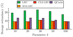
(a) Storage redundancy of the LRU-based policies under SIFT1M trace.

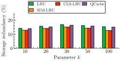
(b) Storage redundancy of the LRU-based policies under Amazon trace.

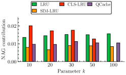
(c) The average gain contribution of the dangling objects under SIFT1M trace.

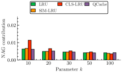
(d) The average gain contribution of the dangling objects under Amazon trace.

Figure 14: Storage redundancy percentage and gain contribution for the different policies. The cache size $h=1000$, and $k\in\{10,20,30,50,100\}$.

XI-B Approximate Index Augmentation

We repeat the sensitivity analysis and show the caching gain when the different policies are augmented with an approximate index, and are allowed to mix the best object that can be served locally and from the server. Figure 15 shows the caching gain for the different caching policies and different values of the cache size $h\in\{50,100,200,500,1000\}$ and $k=10$. Figure 16 shows the caching gain for the different caching policies and different values of the retrieval cost $c_{f}$, that is taken as the average distance to the $i$-th neighbor, $i\in\{2,50,100,500,1000\}$. The cache size is $h=1000$ and $k=10$. Figure 17 shows the caching gain for the different caching policies and different values of $k\in\{10,20,30,50,100\}$ and $h=1000$.

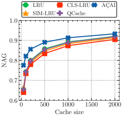
(a) SIFT1M trace

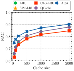
(b) Amazon trace

Figure 15: Caching gain of the different policies when augmented with the approximate index, for different cache sizes $h\in\{50,100,200,500,1000\}$ and $k=10$.

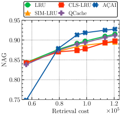
(a) SIFT1M trace

(b) Amazon trace

Figure 16: Caching gain for the different policies and different retrieval cost when augmented with the approximate index. The retrieval cost $c_{f}$ is taken as the average distance to the $i$-th neighbor, $i\in\{2,10,50,100,500,1000\}$. The cache size is $h=1000$ and $k=10$.

(a) SIFT1M trace

(b) Amazon trace

Figure 17: Caching gain for the different policies when augmented with the approximate index. The cache size is $h=1000$, and $k\in\{10,20,30,50,100\}$.

XI-C Computation Time

We provide a comparison of the computation time of the different algorithms in Fig. 18. When the different LRU-like policies are not augmented with a global catalog index in Fig. 18 (a), AÇAI experiences a higher computation time per iteration. When the different LRU-like policies are augmented with a global catalog index in Fig. 18 (b), AÇAI has a similar computation time to the different policies except for the simple vanilla lru policy. Nonetheless, in both settings AÇAI computation time remains comparable and approximately within factor $4$ w.r.t the computation time of the different policies. Due to space limitation we cannot add this figure to the main text.

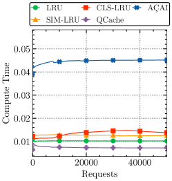
(a)

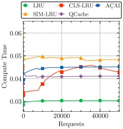
(b)

Figure 18: Time-averaged computation time of AÇAI and the different policies LRU, SIM-LRU, CLS-LRU, and QCache(a) w/o an approximate global catalog index, and (b) w/ an approximate global catalog index. Experiment run over the Amazon trace, cache size $h=1000$, parameter $k=10$, $\eta=10^{-4}$, retrieval cost $c_{f}$ is set to be the distance to the $50$-th closest neighbor in $\mathcal{N}$.

References

• [1] T. Y.-H. Chen, L. Ravindranath, S. Deng, P. Bahl, and H. Balakrishnan, “Glimpse: Continuous, Real-Time Object Recognition on Mobile Devices,” in Proceedings of the 13th ACM Conference on Embedded Networked Sensor Systems, 2015, pp. 155–168.
• [2] Z. Zhou, X. Chen, E. Li, L. Zeng, K. Luo, and J. Zhang, “Edge Intelligence: Paving the Last Mile of Artificial Intelligence With Edge Computing,” Proceedings of the IEEE, vol. 107, no. 8, pp. 1738–1762, 2019.
• [3] S. Venugopal, M. Gazzetti, Y. Gkoufas, and K. Katrinis, “Shadow Puppets: Cloud-level Accurate AI Inference at the Speed and Economy of Edge,” in USENIX Workshop on Hot Topics in Edge Computing (HotEdge 18), Boston, MA, Jul. 2018.
• [4] U. Drolia, K. Guo, J. Tan, R. Gandhi, and P. Narasimhan, “Cachier: Edge-Caching for Recognition Applications,” in 2017 IEEE 37th International Conference on Distributed Computing Systems (ICDCS), 2017, pp. 276–286.
• [5] U. Drolia, K. Guo, and P. Narasimhan, “Precog: Prefetching for Image Recognition Applications at the Edge,” in Proceedings of the Second ACM/IEEE Symposium on Edge Computing, ser. SEC ’17, New York, NY, USA, 2017.
• [6] P. Guo, B. Hu, R. Li, and W. Hu, “FoggyCache: Cross-Device Approximate Computation Reuse,” in Proceedings of the 24th Annual International Conference on Mobile Computing and Networking, ser. MobiCom ’18, New York, NY, USA, 2018, pp. 19–34.
• [7] A. Bellet, A. Habrard, and M. Sebban, “Metric Learning,” Synthesis Lectures on Artificial Intelligence and Machine Learning, vol. 9, no. 1, pp. 1–151, 2015.
• [8] J. Johnson, M. Douze, and H. Jégou, “Billion-Scale Similarity Search with GPUs,” IEEE Transactions on Big Data, vol. 7, no. 3, pp. 535–547, 2021.
• [9] T. Si Salem, G. Neglia, and D. Carra, “AÇAI: Ascent Similarity Caching with Approximate Indexes,” in 2021 33rd International Teletraffic Congress (ITC-33).   IEEE, 2021, pp. 1–9.
• [10] D. Lowe, “Object Recognition from Local Scale-Invariant Features,” in Proceedings of the Seventh IEEE International Conference on Computer Vision, vol. 2, 1999, pp. 1150–1157 vol.2.
• [11] E. Rublee, V. Rabaud, K. Konolige, and G. Bradski, “ORB: An efficient alternative to SIFT or SURF,” in 2011 International Conference on Computer Vision, 2011, pp. 2564–2571.
• [12] G. E. Hinton and R. R. Salakhutdinov, “Reducing the Dimensionality of Data with Neural Networks,” science, vol. 313, no. 5786, pp. 504–507, 2006.
• [13] K. Lin, J. Lu, C.-S. Chen, and J. Zhou, “Learning Compact Binary Descriptors With Unsupervised Deep Neural Networks,” in Proceedings of the IEEE Conference on Computer Vision and Pattern Recognition (CVPR), June 2016.
• [14] P. N. Yianilos, “Data Structures and Algorithms for Nearest Neighbor Search in General Metric Spaces,” in Proceedings of the Fourth Annual ACM-SIAM Symposium on Discrete Algorithms, ser. SODA ’93, USA, 1993, pp. 311–321.
• [15] G. Navarro, “Searching in Metric Spaces by Spatial Approximation,” The VLDB Journal, vol. 11, no. 1, pp. 28–46, aug 2002.
• [16] F. Falchi, C. Lucchese, S. Orlando, R. Perego, and F. Rabitti, “A Metric Cache for Similarity Search,” in Proceedings of the 2008 ACM workshop on Large-Scale distributed systems for information retrieval, 2008, pp. 43–50.
• [17] S. Pandey, A. Broder, F. Chierichetti, V. Josifovski, R. Kumar, and S. Vassilvitskii, “Nearest-Neighbor Caching for Content-Match Applications,” in Proceedings of the 18th International Conference on World Wide Web, ser. WWW ’09, New York, NY, USA, 2009, pp. 441–450.
• [18] G. Neglia, M. Garetto, and E. Leonardi, “Similarity Caching: Theory and Algorithms,” in IEEE/ACM Transactions on Networking, 2021, pp. 1–12.
• [19] P. Sermpezis, T. Giannakas, T. Spyropoulos, and L. Vigneri, “Soft Cache Hits: Improving Performance Through Recommendation and Delivery of Related Content,” IEEE Journal on Selected Areas in Communications, vol. 36, no. 6, pp. 1300–1313, 2018.
• [20] M. Costantini and T. Spyropoulos, “Impact of Popular Content Relational Structure on Joint Caching and Recommendation Policies,” in 2020 18th International Symposium on Modeling and Optimization in Mobile, Ad Hoc, and Wireless Networks (WiOPT), 2020, pp. 1–8.
• [21] D. Crankshaw, X. Wang, G. Zhou, M. J. Franklin, J. E. Gonzalez, and I. Stoica, “Clipper: A Low-Latency Online Prediction Serving System,” in 14th USENIX Symposium on Networked Systems Design and Implementation (NSDI 17), 2017, pp. 613–627.
• [22] G. Paschos, E. Bastug, I. Land, G. Caire, and M. Debbah, “Wireless Caching: Technical Misconceptions and Business Barriers,” IEEE Communications Magazine, vol. 54, no. 8, pp. 16–22, 2016.
• [23] P. Guo and W. Hu, “Potluck: Cross-Application Approximate Deduplication for Computation-Intensive Mobile Applications,” in Proceedings of the Twenty-Third International Conference on Architectural Support for Programming Languages and Operating Systems, 2018, pp. 271–284.
• [24] J. Zhou, O. Simeone, X. Zhang, and W. Wang, “Adaptive Offline and Online Similarity-Based Caching,” IEEE Networking Letters, vol. 2, no. 4, pp. 175–179, 2020.
• [25] A. Sabnis, T. Si Salem, G. Neglia, M. Garetto, E. Leonardi, and R. K. Sitaraman, “GRADES: Gradient Descent for Similarity Caching,” in IEEE Conference on Computer Communications (INFOCOM), 2021.
• [26] M. Garetto, E. Leonardi, and G. Neglia, “Content placement in networks of similarity caches,” Computer Networks, vol. 201, p. 108570, 2021.
• [27] F. Falchi, C. Lucchese, S. Orlando, R. Perego, and F. Rabitti, “Similarity Caching in Large-scale Image Retrieval,” Information Processing & Management, vol. 48, no. 5, pp. 803–818, 2012, large-Scale and Distributed Systems for Information Retrieval.
• [28] G. S. Paschos, A. Destounis, L. Vigneri, and G. Iosifidis, “Learning to Cache With No Regrets,” in IEEE INFOCOM 2019-IEEE Conference on Computer Communications.   IEEE, 2019, pp. 235–243.
• [29] R. Weber, H.-J. Schek, and S. Blott, “A Quantitative Analysis and Performance Study for Similarity-Search Methods in High-Dimensional Spaces,” in Proceedings of the 24rd International Conference on Very Large Data Bases, ser. VLDB ’98, San Francisco, CA, USA, 1998, pp. 194–205.
• [30] A. Andoni and P. Indyk, “Near-Optimal Hashing Algorithms for Approximate Nearest Neighbor in High Dimensions,” in 2006 47th Annual IEEE Symposium on Foundations of Computer Science (FOCS’06), 2006, pp. 459–468.
• [31] A. Babenko and V. Lempitsky, “The Inverted Multi-Index,” IEEE Transactions on Pattern Analysis and Machine Intelligence, vol. 37, no. 6, pp. 1247–1260, 2015.
• [32] Y. A. Malkov and D. A. Yashunin, “Efficient and Robust Approximate Nearest Neighbor Search Using Hierarchical Navigable Small World Graphs,” IEEE Transactions on Pattern Analysis and Machine Intelligence, vol. 42, no. 4, pp. 824–836, 2020.
• [33] M. Aumüller, E. Bernhardsson, and A. Faithfull, “ANN-Benchmarks: A Benchmarking Tool for Approximate Nearest Neighbor Algorithms,” in Similarity Search and Applications, C. Beecks, F. Borutta, P. Kröger, and T. Seidl, Eds., Cham, 2017, pp. 34–49.
• [34] S. Ioannidis, L. Massoulie, and A. Chaintreau, “Distributed Caching over Heterogeneous Mobile Networks,” in Proceedings of the ACM SIGMETRICS International Conference on Measurement and Modeling of Computer Systems, ser. SIGMETRICS ’10, New York, NY, USA, 2010, pp. 311–322.
• [35] S. Ioannidis and E. Yeh, “Adaptive Caching Networks with Optimality Guarantees,” ACM SIGMETRICS Performance Evaluation Review, vol. 44, no. 1, pp. 113–124, 2016.
• [36] T. Si Salem, G. Castellano, G. Neglia, F. Pianese, and A. Araldo, “Towards Inference Delivery Networks: Distributing Machine Learning with Optimality Guarantees,” in 2021 19th Mediterranean Communication and Computer Networking Conference (MedComNet), 2021, pp. 1–8.
• [37] S. Shalev-Shwartz, “Online Learning and Online Convex Optimization,” Machine Learning, vol. 4, no. 2, pp. 107–194, 2011.
• [38] T. Si Salem, G. Neglia, and S. Ioannidis, “No-Regret Caching via Online Mirror Descent,” in IEEE International Conference on Communications (ICC), 2021.
• [39] T. Si Salem, G. Neglia, and S. Ioannidis, “No-Regret Caching via Online Mirror Descent,” preprint Arxiv:2101.12588, 2021.
• [40] S. Mukhopadhyay and A. Sinha, “Online Caching with Optimal Switching Regret,” in 2021 IEEE International Symposium on Information Theory (ISIT), 2021, pp. 1546–1551.
• [41] K. Shanmugam, N. Golrezaei, A. G. Dimakis, A. F. Molisch, and G. Caire, “FemtoCaching: Wireless Content Delivery Through Distributed Caching Helpers,” IEEE Transactions on Information Theory, vol. 59, no. 12, pp. 8402–8413, 2013.
• [42] G. Neglia, E. Leonardi, G. I. Ricardo, and T. Spyropoulos, “A Swiss Army Knife for Dynamic Caching in Small Cell Networks,” IEEE/ACM Transactions on Networking, 9 August 2021, 2021.
• [43] S. Bubeck, “Convex Optimization: Algorithms and Complexity,” Foundations and Trends in Machine Learning, vol. 8, no. 3-4, pp. 231–357, Nov. 2015.
• [44] J. Byrka, T. Pensyl, B. Rybicki, A. Srinivasan, and K. Trinh, “An Improved Approximation for k-median, and Positive Correlation in Budgeted Optimization,” in Proceedings of the 2015 Annual ACM-SIAM Symposium on Discrete Algorithms (SODA), 2017, pp. 737–756.
• [45] T. Lorido-Botran, J. Miguel-Alonso, and J. A. Lozano, “A Review of Auto-scaling Techniques for Elastic Applications in Cloud Environments,” Journal of Grid Computing, vol. 12, no. 4, pp. 559–592, 2014.
• [46] N. Carlsson and D. Eager, “Worst-Case Bounds and Optimized Cache on Mth Request Cache Insertion Policies under Elastic Conditions,” ACM SIGMETRICS Performance Evaluation Review, vol. 46, no. 3, pp. 37–38, jan 2019.
• [47] D. Carra, G. Neglia, and P. Michiardi, “Elastic Provisioning of Cloud Caches: A Cost-Aware TTL Approach,” IEEE/ACM Transactions on Networking, vol. 28, no. 3, pp. 1283–1296, 2020.
• [48] M. Mitzenmacher and E. Upfal, Probability and Computing: Randomized Algorithms and Probabilistic Analysis.   USA: Cambridge University Press, 2005.
• [49] A. Krause and D. Golovin, “Submodular Function Maximization,” in Tractability: Practical Approaches to Hard Problems, 2014, pp. 71–104.
• [50] F. Radlinski, R. Kleinberg, and T. Joachims, “Learning Diverse Rankings with Multi-Armed Bandits,” in Proceedings of the 25th international conference on Machine learning, 2008, pp. 784–791.
• [51] R. Kleinberg, A. Slivkins, and E. Upfal, “Multi-Armed Bandits in Metric Spaces,” in Proceedings of the fortieth annual ACM symposium on Theory of computing, 2008, pp. 681–690.
• [52] J.-Y. Audibert, R. Munos, and C. Szepesvári, “Exploration–Exploitation Tradeoff Using Bariance Estimates in Multi-Armed Bandits,” Theoretical Computer Science, vol. 410, no. 19, pp. 1876–1902, 2009.
• [53] W. Chu, L. Li, L. Reyzin, and R. Schapire, “Contextual Bandits with Linear Payoff Functions,” in Proceedings of the Fourteenth International Conference on Artificial Intelligence and Statistics.   JMLR Workshop and Conference Proceedings, 2011, pp. 208–214.
• [54] A. Agarwal, D. Hsu, S. Kale, J. Langford, L. Li, and R. Schapire, “Taming the Monster: a Fast and Simple Algorithm for Contextual Bandits,” in International Conference on Machine Learning.   PMLR, 2014, pp. 1638–1646.
• [55] M. Dudik, D. Hsu, S. Kale, N. Karampatziakis, J. Langford, L. Reyzin, and T. Zhang, “Efficient Optimal Learning for Contextual Bandits,” in Proceedings of the Twenty-Seventh Conference on Uncertainty in Artificial Intelligence, 2011, pp. 169–178.
• [56] R. Bhattacharjee, S. Banerjee, and A. Sinha, “Fundamental Limits on the Regret of Online Network-Caching,” Proceedings of the ACM on Measurement and Analysis of Computing Systems, vol. 4, no. 2, jun 2020.
• [57] Y. Li, T. Si Salem, G. Neglia, and S. Ioannidis, “Online Caching Networks with Adversarial Guarantees,” Proceedings of the ACM on Measurement and Analysis of Computing Systems, vol. 5, no. 3, pp. 1–39, 2021.
• [58] L. Chen, H. Hassani, and A. Karbasi, “Online Continuous Submodular Maximization,” in International Conference on Artificial Intelligence and Statistics, 2018, pp. 1896–1905.
• [59] E. Hazan et al., “Introduction to online convex optimization,” Foundations and Trends® in Optimization, vol. 2, no. 3-4, pp. 157–325, 2016.
• [60] G. L. Nemhauser and L. A. Wolsey, “Best Algorithms for Approximating the Maximum of a Submodular Set Function,” Mathematics of Operations Research, vol. 3, no. 3, pp. 177–188, 1978.
• [61] A. Sabnis, T. Si Salem, G. Neglia, M. Garetto, E. Leonardi, and R. K. Sitaraman, “GRADES: Gradient Descent for Similarity Caching,” in IEEE Conference on Computer Communications (INFOCOM), 2021.
• [62] E. G. Coffman and P. J. Denning, Operating Systems Theory.   Prentice Hall, 1973, vol. 973.
• [63] S. Diamond and S. Boyd, “CVXPY: A Python-Embedded Modeling Language for Convex Optimization,” Journal of Machine Learning Research, vol. 17, no. 1, pp. 2909–2913, jan 2016.
• [64] H. Jégou, M. Douze, and C. Schmid, “Product Quantization for Nearest Neighbor Search,” IEEE Transactions on Pattern Analysis and Machine Intelligence, vol. 33, no. 1, pp. 117–128, 2011.
• [65] J. McAuley, C. Targett, Q. Shi, and A. van den Hengel, “Image-Based Recommendations on Styles and Substitutes,” in Proceedings of the 38th International ACM SIGIR Conference on Research and Development in Information Retrieval, ser. SIGIR ’15, New York, NY, USA, 2015, pp. 43–52.
• [66] U. Khandelwal, O. Levy, D. Jurafsky, L. Zettlemoyer, and M. Lewis, “Generalization through Memorization: Nearest Neighbor Language Models,” in International Conference on Learning Representations (ICLR), 2020.
• [67] M. Zinkevich, “Online Convex Programming and Generalized Infinitesimal Gradient Ascent,” in Proceedings of the Twentieth International Conference on International Conference on Machine Learning, ser. ICML’03.   AAAI Press, 2003, pp. 928–935.
• [68] T. Si Salem, G. Castellano, G. Neglia, F. Pianese, and A. Araldo, “Towards Inference Delivery Networks: Distributing Machine Learning with Optimality Guarantees,” preprint arXiv:2105.02510, 2021.
• [69] B. S. Mordukhovich and N. M. Nam, “Geometric Approach to Subdifferential Calculus,” Optimization, vol. 66, no. 6, pp. 839–873, 2017.
• [70] R. T. Rockafellar, Convex Analysis.   Princeton University Press, 2015.