Partial Identification and Inference in Duration Models with Endogenous Censoring

Abstract

This paper studies identification and inference in transformation models with endogenous censoring. Many kinds of duration models, such as the accelerated failure time model, proportional hazard model, and mixed proportional hazard model, can be viewed as transformation models. We allow the censoring of a duration outcome to be arbitrarily correlated with observed covariates and unobserved heterogeneity. We impose no parametric restrictions on either the transformation function or the distribution function of the unobserved heterogeneity. In this setting, we develop bounds on the regression parameters and the transformation function, which are characterized by conditional moment inequalities involving U-statistics. We provide inference methods for them by constructing an inference approach for conditional moment inequality models in which the sample analogs of moments are U-statistics. We apply the proposed inference methods to evaluate the effect of heart transplants on patients’ survival time using data from the Stanford Heart Transplant Study. Keywords: Partial identification, duration models, transformation models, censoring, conditional moment inequality.
JEL codes: C14, C24, C41.

1 Introduction

Duration models are widely used in various empirical studies in economics and biomedical sciences, where outcomes of interest are durations up to the occurrence of some event. Durations of interest in economics include unemployment duration, strike duration, insurance claim duration, and the duration until the purchase of a durable good.

In practice, duration data are often censored. For example, unemployment duration is likely to be censored due to some individuals dropping out of the survey, due to attrition say. Dealing with censoring has been a substantial challenge in duration analysis, and various methods have been proposed. A standard approach is to assume that censoring is independent of unobserved heterogeneity (conditional or unconditional on observed characteristics). Studies employing this approach include Cox (1972), Powell (1984), Ying et al. (1995), Yang (1999), Honoré et al. (2002), Hong and Tamer (2003), and Khan and Tamer (2007), among others. However, in many cases, justifying this independence assumption is difficult. For example, in unemployment duration analysis, unemployed individuals with low motivation to find a job may tend to drop out of the survey at an early stage. Szydłowski (2019) presents a number of examples where censoring is correlated with unobserved heterogeneity (i.e., censoring is endogenous).

In this paper, we study identification and inference in transformation models in the presence of endogenous censoring. The transformation model is expressed as

$$Y^{\ast}=\Lambda(X^{\prime}\beta_{0}+U),$$ (1.1)

where $\Lambda$ is a non-degenerate monotone function; $Y^{\ast}$ is a dependent variable, which represents a duration outcome in this paper; $X$ is a $k$-dimensional vector of observed covariates, where $k\geq 2$; $\beta_{0}$ denotes a $k$-vector of regression parameters; and $U$ is unobserved heterogeneity that is independent of $X$. Many kinds of duration models, such as the accelerated failure time model, proportional hazard model, and mixed proportional hazard (MPH) model, can be viewed as transformation models. In this paper, we consider a nonparametric transformation model in which neither the transformation function nor the distribution function of the unobserved heterogeneity is parametrically specified. One important model represented by the nonparametric transformation model is the nonparametric MPH model in which neither a baseline hazard function nor the distribution function of the unobserved heterogeneity is parametrically specified.

Allowing for endogenous censoring, we develop bounds on the regression parameters $\beta_{0}$ and transformation function $\Lambda$ in model (1.1). To the best of our knowledge, this is the first work to derive bounds on $\beta_{0}$ and $\Lambda$ in the nonparametric transformation model with endogenous censoring. The construction of the bounds is built on the rank properties of the nonparametric transformation model studied by Han (1987) and Chen (2002). Han (1987) shows that if there is no censoring, at least one element of $X$ has full-support on the real line, and $X$ is full-rank, the regression parameters are point-identified up to scale by looking at the rank correlation between the outcomes and covariates. In the presence of endogenous censoring, we develop bounds on $\beta_{0}$ by supposing that, in the rank property studied by Han (1987), each censored outcome takes an infinitely large value or is equal to the censoring time. This reflects the fact that concerning each censored outcome, all we know is that it may take any value larger than censoring time. When $\Lambda$ is strictly increasing, a lower bound on $\Lambda$ is also attained by incorporating endogenous censoring into the rank property studied by Chen (2002). Once the bounds on the regression parameters and the transformation function are obtained, we can also derive bounds on the distribution function of the unobserved heterogeneity $U$.

The bounds on $\beta_{0}$ and $\Lambda$ are characterized by conditional moment inequalities whose sample moments are U-statistics. Based on these conditional moment inequalities, we construct inference methods for these parameters by extending the inference approach of Andrews and Shi (2013) for conditional moment inequality models to the case of U-statistics. The proposed inference approach can be applied not only to this work but also to other works involving conditional moment inequalities and U-statistics. In this sense, this paper also contributes to the literature on inference for conditional moment inequality models.

The bounded sets of the parameters proposed in this paper are not necessarily sharp identified sets. On the other hand, using concepts from random set theory (e.g., Beresteanu et al. (2011, 2012)), we also characterize the sharp identified set of the regression parameters. However, constructing a feasible inference method based on it is difficult, whereas the proposed sets are tractable to construct feasible inference methods. In the paper, we also discuss conditions under which the proposed set of $\beta_{0}$ approaches the sharp identified set.

This paper is mostly related to works that study endogenous censoring. Khan and Tamer (2009), Khan et al. (2011, 2016), Li and Oka (2015), and Fan and Liu (2018) study identification and estimation of parameters in quantile regression models with endogenous censoring. For cross-sectional linear quantile regression models, Khan and Tamer (2009) provide a point identification result for the linear coefficients under a certain support condition, while Khan et al. (2011) provide a partial identification result without this support condition. Under censoring characterized by a certain copula, Fan and Liu (2018) partially identify the linear coefficients of the same model. Li and Oka (2015) and Khan et al. (2016) consider panel quantile regression models with endogenous censoring and provide partial identification results. In contrast to these works, the identification result in this paper does not rely on quantile modeling, copula characterization of censoring, or panel data. Aside from quantile models, Szydłowski (2019) considers the parametric MPH model and proposes a sharp identified set and inference method for its parameters. While Szydłowski (2019) considers the parametric MPH model, we consider the nonparametric one, which is robust to misspecification of the hazard function or the distribution function of unobserved heterogeneity.

For competing risks models, Honoré and Lleras-Muney (2006) partially identify the parameters in the accelerated failure time model, and Kim (2018) derives computationally tractable bounds on distributions of latent durations by exploiting the discreteness of observed durations. In this paper, we allow for continuous observed durations and do not specify competing risks. In a sample selection model, Honoré and Hu (2020) obtain the sharp identified set of linear regression coefficients by imposing a particular structure on the sample selection.

The remainder of this paper is structured as follows. Section 2 describes the setup and assumptions and then provides the main results to develop bounds on the regression parameters and the transformation function. We also characterize the sharp identified set of the regression parameters and compare it to our proposed superset. Section 3 provides an inference method for the regression parameters and derives its asymptotic properties. A joint inference method for the regression parameters and the transformation function is presented in Appendix C. Section 4 presents numerical examples and Monte Carlo simulation results. The numerical examples show how the bounds on the regression parameters and transformation function vary depending on the degree of censoring and the support of covariates. The Monte Carlo simulation results show the finite sample properties of the proposed inference method for the regression parameters. Section 5 presents an empirical illustration, where we apply our proposed inference methods to evaluate the effect of heart transplants on patients’ survival duration using data from the Stanford Heart Transplant Study. We conclude this paper with some remarks in Section 6. All proofs are presented in Appendices A and B. Some additional numerical examples and Monte Carlo simulation results are presented in the supplementary material to this paper.

2 Model and Identification

We first describe the setting of the paper and provide conditions to develop bounds on the regression parameters in Section 2.1. Subsequently, in Section 2.2, we present the main result to construct bounds on the regression parameters. In Section 2.3, we characterize the sharp identified set of the regression parameters using concepts from random set theory, and compare this with our proposed superset. Section 2.4 derives bounds on the transformation function and the distribution of the unobserved heterogeneity.

2.1 Model

We consider the transformation model in the form of (1.1). In the model, we do not specify the transformation function $\Lambda$ or the distribution function of the unobserved heterogeneity, which we denote by $F_{U}$. Because of this, we impose location and scale normalizations. For the location normalization, we suppose that the constant term is equal to zero (i.e., $X$ does not contain a constant term). For the scale normalization, we suppose that the absolute value of the first component of $\beta_{0}$ is equal to one (i.e., $\left|\beta_{0,1}\right|=1$), where $\beta_{0,j}$ denotes the $j$-th component of $\beta_{0}$. Later, in Section 2.4, we impose an additional location normalization to fix $\Lambda$. Let $B\equiv\{-1,1\}\times\mathbb{R}^{k-1}$ denote the normalized regression parameter space. Our first main focus is on the identification of and inference on the normalized regression parameters $\beta_{0}$ in $B$.

The transformation model contains many kinds of duration models as its special cases: the accelerated failure time model, Cox’s proportional hazard model, and the MPH model. In particular, the nonparametric MPH model is an important duration model represented by a nonparametric transformation model. The MPH model extends Cox’s proportional hazard model by incorporating individual unobserved heterogeneity. Since introduced in Lancaster (1979), the MPH model has been widely used in various empirical studies in economics. In the nonparametric MPH model, the normalized regression parameters $\beta_{0}$ can be interpreted as the logs of the scale-normalized hazard ratios (see, e.g., Lancaster (1990)).

When data are subject to censoring, the duration outcome $Y^{\ast}$ cannot always be observed. Instead, for unit $i=1,\ldots,n$, we observe $W_{i}=\left(Y_{0i},D_{i},X_{i}\right)$ such that $Y_{0i}=\mbox{min}\left\{Y_{i}^{\ast},C_{i}\right\}$ and $D_{i}=I\left[Y_{i}^{\ast}\leq C_{i}\right]$, where $C_{i}$ is a random censoring variable and $I\left[\cdot\right]$ denotes the indicator function. $D_{i}$ is a censoring indicator that takes the value zero if $Y_{i}^{\ast}$ is censored and the value one if $Y_{i}^{\ast}$ is observed. Note that we consider right censoring in the paper, but all the results presented below are easily extendable to left and interval censoring. Using $D_{i}$, $Y_{0i}$ can be expressed as $Y_{0i}=D_{i}Y_{i}^{\ast}+(1-D_{i})C_{i}$. Let $P$ denote the distribution function of a vector of random variables $\left(X,U,C\right)$ and $\mathcal{X}\subseteq\mathbb{R}^{k}$ denote the support of $X$.

Throughout this paper, we suppose that the following assumptions hold.

Assumption 2.1.

$\Lambda$ is a non-degenerate monotonically increasing function.

Assumption 2.2.

The vectors $\left(Y_{i}^{\ast},C_{i},X_{i}\right)$, $i=1,\ldots,n$, are independent and identically distributed (i.i.d) as $(Y^{\ast},X,C)$ where $Y^{\ast}$ is distributed according to the latent transformation model (1.1) and the support of $X$ is $\mathcal{X}$.

Assumption 2.3.

$U$ is independent of $X$.

Note that Assumption 2.3 does not restrict the relationship between $U$ and $C$, allowing for endogenous censoring.

2.2 Identification of the Regression Parameters

This section constructs bounds on the regression parameters $\beta_{0}$. The construction is based on a rank property of the latent outcome $Y^{*}$ and the regression part $X^{\prime}\beta_{0}$ in the transformation model (1.1). For explanatory purposes, we first introduce the point identification result of Han (1987) in the absence of censoring.

Han (1987) supposes that there is no censoring (i.e., $Y^{\ast}$ is always observed). In this case, under Assumptions 2.1–2.3, a full-support condition on an element of $X$, a full-rank condition on $X$, and a continuous distribution of $U$, he shows that $\beta_{0}$ uniquely satisfies the following rank property,

$$x_{i}^{\prime}\beta_{0}\geq x_{j}^{\prime}\beta_{0}\Rightarrow P(Y_{i}^{\ast}\geq Y_{j}^{\ast}\mid x_{i},x_{j})\geq\frac{1}{2}$$ (2.1)

for all $(x_{i},x_{j})\in\mathcal{X}^{2}$, where $P(\cdot\mid x_{i},x_{j})$ denotes the conditional probability given $(X_{i},X_{j})=(x_{i},x_{j})$. This rank property means that, for any given pair of $(x_{i},x_{j})$, the probability that $Y_{i}^{\ast}$ is larger than or equal to $Y_{j}^{\ast}$ is greater than or equal to 1/2 if and only if $x_{i}^{\prime}\beta_{0}$ is larger than or equal to $x_{j}^{\prime}\beta_{0}$. Then $\beta_{0}$ is the unique value in $B$ that satisfies this rank relation for any pair of $(x_{i},x_{j})\in\mathcal{X}^{2}$. In other words, for any $\beta\neq\beta_{0}$, there exists at least one pair $(x_{i},x_{j})\in\mathcal{X}^{2}$ that violates the rank relation (2.1).

In this paper, we suppose that censoring exists and it may be endogenous. Hence, we cannot always observe $Y_{i}^{\ast}$ and do not have any information about the censoring mechanism. The censoring variable $C_{i}$ may be arbitrarily correlated with the observed covariates $X_{i}$ and unobserved heterogeneity $U_{i}$.

In this situation, we can still construct bounds on the regression parameters $\beta_{0}$. Let $Y_{1i}\equiv D_{i}Y_{i}^{\ast}+(1-D_{i})(+\infty)$, which is an outcome variable that takes an arbitrary large value when the primary outcome is censored. Recall that $Y_{0i}=D_{i}Y_{i}+(1-D_{i})C_{i}$. Then because $P(Y_{1i}\geq Y_{0j}\mid x_{i},x_{j})\geq P(Y_{i}^{\ast}\geq Y_{j}^{\ast}\mid x_{i},x_{j})$ holds for all $(x_{i},x_{j})\in\mathcal{X}^{2}$, the following rank property holds from (2.1):

$$x_{i}^{\prime}\beta_{0}\geq x_{j}^{\prime}\beta_{0}\Rightarrow P(Y_{1i}\geq Y_{0j}\mid x_{i},x_{j})\geq\frac{1}{2}$$ (2.2)

for all $(x_{i},x_{j})\in\mathcal{X}^{2}$. Therefore, defining

$$B_{I}\equiv\{\beta\in B\mid\ \mbox{$x_{i}^{\prime}\beta\geq x_{j}^{\prime}\beta\Rightarrow P\left(Y_{1i}\geq Y_{0j}\mid x_{i},x_{j}\right)\geq\frac{1}{2}$ for all \mbox{$(x_{i},x_{j})\in\mathcal{X}^{2}$}}\},$$

$\beta_{0}$ is contained in $B_{I}$. This set is derived from a worst-case analysis where we suppose that censored outcomes may take extreme values, $C$ or $+\infty$, for any given value of $x$. This reflects the fact that concerning each censored outcome, all we know is that it may take any value at least larger than its censored time.

The following assumption ensures that $B_{I}$ is a proper subset of $B(=\{-1,1\}\times\mathbb{R}^{k-1})$.

Assumption 2.4.

Let $\widetilde{\mathcal{X}}^{2}\equiv\{(x_{i},x_{j})\in\mathcal{X}^{2}\mid P(Y_{1i}\geq Y_{0j}\mid x_{i},x_{j})<\frac{1}{2}\}$. Then $P((X_{i},X_{j})\in\widetilde{\mathcal{X}}^{2})>0$.

The following theorem summarizes the main result in this section.

Theorem 2.1.

Under Assumptions 2.1–2.4, $\beta_{0}\in B_{I}\subset B$ a.s.

A proof of this theorem is given in Appendix A. We make several remarks about this theorem. First, in this theorem, we do not impose a full-support condition on an element of $X$, in contrast to many works in the semiparametric literature, as we no longer focus on point identification. A full-rank condition on $X$ is necessary (but not sufficient) for $B_{I}$ to be bounded. Second, as we will see in the following subsection, $B_{I}$ is not a sharp identified set. However, this set is easy to compute and to construct a feasible inference method, as we will see in Section 3. The following subsection shows how the sharp identified set can be characterized, and its computational difficulty.

2.3 Characterization of the Sharp Identified Set

In this section, we illustrate a way to characterize the sharp identified set using concepts from random set theory. Subsequently, we compare the sharp identified set with $B_{I}$. This comparison clarifies why $B_{I}$ is not a sharp set and in which situations $B_{I}$ approaches the sharp set. For the definitions and notations for random set theory used in this section, see, for example, Molchanov (2005) or Beresteanu et al. (2012, Appendix A). Throughout this section, for any variable $A$, we denote by $\tilde{A}$ an independent copy of $A$.

Using concepts from random set theory, we can characterize the incomplete information for the latent outcome variable $Y^{\ast}$. For any random variable $A$, let $A_{x}$ denote a random variable that has the conditional distribution of $A$ given $X=x$. Then, for a given $x\in\mathcal{X}$, what we observe for the latent outcome variable in the presence of endogenous censoring can be expressed as the random set $\mathcal{Y}_{x}$ defined as

$$\mathcal{Y}_{x} = \begin{cases}\begin{array}[]{c}\{Y_{x}^{\ast}\}\\ (C_{x},+\infty)\end{array}&\begin{array}[]{c}\mbox{if}\ D_{x}=1\\ \mbox{otherwise}\end{array}\end{cases},$$

where $Y_{x}^{\ast}$ and $C_{x}$ are, respectively, a latent outcome and a censoring variable given $X=x$; $D_{x}=I\left[Y_{x}^{\ast}\leq C_{x}\right]$ is a censoring indicator given $X=x$. Hence, all the information for the latent outcome variable can be expressed by stating that $Y_{x}^{\ast}\in\mbox{Sel}(\mathcal{Y}_{x})$. Let $B_{0}$ denote the sharp identified set of $\beta_{0}$. Throughout this section, we suppose that the full-support condition on one element of $X$, the full-rank condition on $X$, and the continuity of $F_{U}$ hold to ensure the sharp identification result.

Combining the above random set representation with Han’s (1987) point identification result that $\beta_{0}$ uniquely satisfies the the rank property (2.1) for all $(x_{i},x_{j})\in\mathcal{X}^{2}$, the sharp identified set $B_{0}$ is characterized as the set of $\beta$ such that there exists a family of pairs of selections $(Y_{x_{i}},\tilde{Y}_{x_{j}})\in\mbox{Sel}(\mathcal{Y}_{x_{i}})\times\mbox{Sel}(\widetilde{\mathcal{Y}}_{x_{j}})$ over $(x_{i},x_{j})\in{\cal{X}}^{2}$ that satisfy the following:

$$x_{i}^{\prime}\beta\geq x_{j}^{\prime}\beta\Leftrightarrow P(Y_{x_{i}}\geq\tilde{Y}_{x_{j}})\geq\frac{1}{2}$$ (2.3)

for all $(x_{i},x_{j})\in{\cal X}^{2}$, where $\widetilde{\mathcal{Y}}_{x}$ is the random set of $\tilde{Y}_{x}$. Therefore, $B_{0}$ is characterized as

$$B_{0}=\left\{\beta\in B\mid\exists\left\{(Y_{x_{i}},\tilde{Y}_{x_{j}})\in\mbox{Sel}(\mathcal{Y}_{x_{i}})\times\mbox{Sel}(\widetilde{\mathcal{Y}}_{x_{j}})\right\}_{(x_{i},x_{j})\in{\cal{X}}^{2}},\forall(x_{i},x_{j})\in{\cal X}^{2},\mbox{(\ref{eq:rank inequality_random set}) holds}\right\}.$$ (2.4)

We next look at how the proposed set $B_{I}$ can be characterized by the random set. Given $x\in\mathcal{X}$, by definition, $Y_{1x}$ and $Y_{0x}$ satisfy (i) $Y_{1x},Y_{0x}\in\mbox{Sel}(\mathcal{Y}_{x})$ a.s. and (ii) $Y_{0x}\leq Y_{x}\leq Y_{1x}$ a.s. for all $Y_{x}\in\mbox{Sel}(\mathcal{Y}_{x})$. Thus for any given pair $(x_{i},x_{j})\in\mathcal{X}^{2}$, the parameter set

$$\{\beta\in B\mid\mbox{$x_{i}^{\prime}\beta\geq x_{j}^{\prime}\beta\Rightarrow P\left(Y_{1i}\geq Y_{0j}\mid x_{i},x_{j}\right)\geq\frac{1}{2}$}\}$$

is equivalent to

$$\left\{\beta\in B\mid\exists\left(Y_{x_{i}},\tilde{Y}_{x_{j}}\right)\in\mbox{Sel}(\mathcal{Y}_{x_{i}})\times\mbox{Sel}(\widetilde{\mathcal{Y}}_{x_{j}}),\mbox{(\ref{eq:rank inequality_random set}) holds}\right\},$$

which is the set of $\beta$ such that for the fixed $(x_{i},x_{j})$, there exists a pair of selections $\left(Y_{x_{i}},\tilde{Y}_{x_{j}}\right)\in\mbox{Sel}(\mathcal{Y}_{x_{i}})\times\mbox{Sel}(\widetilde{\mathcal{Y}}_{x_{j}})$ that satisfies the inequality (2.3). Therefore, $B_{I}$ is characterized as the set of $\beta$ such that for any pair $(x_{i},x_{j})\in{\cal{X}}^{2}$, there exists a pair of selections $\left(Y_{x_{i}},\tilde{Y}_{x_{j}}\right)\in\mbox{Sel}(\mathcal{Y}_{x_{i}})\times\mbox{Sel}(\widetilde{\mathcal{Y}}_{x_{j}})$ that satisfy the inequality (2.3). Formally, $B_{I}$ is characterized as

$$B_{I}=\left\{\beta\in B\mid\forall(x_{i},x_{j})\in{\cal X}^{2},\exists\left(Y_{x_{i}},\tilde{Y}_{x_{j}}\right)\in\mbox{Sel}(\mathcal{Y}_{x_{i}})\times\mbox{Sel}(\widetilde{\mathcal{Y}}_{x_{j}}),\mbox{(\ref{eq:rank inequality_random set}) holds}\right\}.$$ (2.5)

The difference between (2.4) and (2.5) (i.e., the different orders of “$\forall(x_{i},x_{j})\in{\cal X}^{2}$” and “$\exists\left(Y_{x_{i}},\tilde{Y}_{x_{j}}\right)\in\mbox{Sel}(\mathcal{Y}_{x_{i}})\times\mbox{Sel}(\widetilde{\mathcal{Y}}_{x_{j}})$” in (2.4) and (2.5)) shows that $B_{0}$ is contained in $B_{I}$, but $B_{0}$ does not necessary contain $B_{I}$. Hence $B_{I}$ is not necessarily a sharp set. Some intuition for the non-sharpness of $B_{I}$ is as follows. Fix a triple $\left(x_{i},x_{j},x_{k}\right)\in\mathcal{X}^{3}$ and $\beta\in B$ such that $x_{i}^{\prime}\beta\leq x_{j}^{\prime}\beta\leq x_{k}^{\prime}\beta$. When we check whether $\beta\in B_{I}$ through the rank property (2.1), in comparing $x_{j}$ and $x_{k}$, we suppose that the latent outcome variable $Y_{x_{j}}^{\ast}$ takes its smallest value, $C_{x_{j}}$; whereas, in comparing $x_{j}$ and $x_{i}$, we suppose that $Y_{x_{j}}^{\ast}$ takes its largest value, $+\infty$. However, when we check whether $\beta\in B_{0}$ through the characterization of (2.4), we compare fixed selections $Y_{x}\in\mbox{Sel}(\mathcal{Y}_{x})$ over all $x\in\cal{X}$; that is, $Y_{x_{j}}$ does not change when comparing different $\tilde{Y}_{x_{i}}$ over $x_{i}\in\cal{X}$. This difference explains why $B_{I}$ is larger than $B_{0}$.

Remark 2.1.

Although we could characterize the sharp set $B_{0}$ as (2.4), it is hard to compute. When examining whether a certain $\beta$ is contained in $B_{0}$, one would have to search for the existence of measurable selections $Y_{x}\in\mbox{Sel}(\mathcal{Y}_{x})$ for all $x\in\cal{X}$ that satisfy the rank inequality (2.3) for all pairs $(x_{i},x_{j})\in\mathcal{X}^{{}^{2}}$. In contrast, $B_{I}$ is much easier to compute. For this reason, we focus on $B_{I}$ in this paper rather than the sharp set.

Remark 2.2.

There are some situations when $B_{I}$ is close to $B_{0}$. The first case is when censoring does not occur frequently. If censoring is unlikely to occur given any $x\in\mathcal{X}$, measurable selections of $\mathcal{Y}_{x}$ correspond to a single measurable selection $Y_{x}^{\ast}$ with high probability. The second case is when $Y_{x}^{\ast}$ is not censored at small values for each $x\in\mathcal{X}$; that is, $C_{x}$ takes a large value when $Y_{x}^{\ast}$ is censored. In this case, for each $x\in\mathcal{X}$, the random interval $(C_{x},+\infty)$ in the definition of $\mathcal{Y}_{x}$ is narrow, and hence the difference between (2.4) and (2.5) does not make much difference between $B_{I}$ and $B_{0}$. In the empirical example of the heart transplantation study in Section 5, this case corresponds to the case when each patient is unlikely to drop out of the study at an early stage.

2.4 Identification of the Transformation Function

We next develop a lower bound on the transformation function in the presence of endogenous censoring. Knowing about the transformation function enables us to infer the type of duration model. We here suppose that $\Lambda$ is strictly monotonic.

Assumption 2.5.

$\Lambda$ is a strictly increasing function.

Let $T\equiv\Lambda^{-1}$. We call $T$ the transformation function when no confusion arises. As an additional location normalization to fix $T$, we suppose $T(\tilde{y})=0$ for some specific outcome value $\tilde{y}<\infty$. We now construct a bound on the normalized $T(y)$ at a particular value of $y\in\mathbb{R}$.

Construction of the bound is built on the rank property studied by Chen (2002). In the case of no censoring, provided that Assumptions 2.2–2.3 and 2.5 hold and that the true regression parameters $\beta_{0}$ are given, Chen (2002) shows that $T\left(y\right)$ satisfies the following rank property:

$$x_{i}^{\prime}\beta_{0}-x_{j}^{\prime}\beta_{0}\geq T(y)\Rightarrow P\left(Y_{i}^{\ast}\geq y\mid x_{i}\right)\geq P\left(Y_{j}^{\ast}\geq\tilde{y}\mid x_{i}\right)$$ (2.6)

for all $(x_{i},x_{j})\in{\cal X}^{2}$, where we recall that $\tilde{y}$ is such that $T\left(\tilde{y}\right)=0$ for the location normalization. Moreover, supposing further that the full-support and full-rank conditions on $X$ and the continuity of $F_{U}$ hold, Chen (2002) shows that $T\left(y\right)$ can be point identified as the minimum value of $t$ that satisfies the inequality (2.6) with $t$ in place of $T(y)$ for all $(x_{i},x_{j})\in\mathcal{X}^{2}$. Chen (2002) also provides an inference method based on this identification result.

In the presence of endogenous censoring, we can construct a lower bound on $T\left(y\right)$ using a similar idea to that presented in Section 2.2. If $\beta_{0}$ were given, because $P(Y_{1i}\geq y\mid x_{i})\geq P(Y_{i}^{\ast}\geq y\mid x_{i})$ and $P(Y_{j}^{\ast}\geq y\mid x_{j})\geq P(Y_{0j}\geq y\mid x_{j})$ hold for all $(x_{i},x_{j})\in\mathcal{X}^{2}$, it follows from (2.6) that $T\left(y\right)$ is contained in the following set:

$$\left\{t\in\mathbb{R}:x_{i}^{\prime}\beta_{0}-x_{j}^{\prime}\beta_{0}\geq t\Rightarrow P\left(Y_{1i}\geq y\mid x_{i}\right)\geq P\left(Y_{0j}\geq\tilde{y}\mid x_{i}\right)\ \mbox{for all}\ (x_{i},x_{j})\in{\cal X}^{2}\right\}.$$ (2.7)

In the presence of endogenous censoring, we cannot point identify $\beta_{0}$; instead, we have $B_{I}$ which contains $\beta_{0}$. Thus, letting

$$T_{I,\beta}\left(y\right)\equiv\left\{t\in\mathbb{R}:x_{i}^{\prime}\beta-x_{j}^{\prime}\beta\geq t\Rightarrow P\left(Y_{1i}\geq y\mid x_{i}\right)\geq P\left(Y_{0j}\geq\tilde{y}\mid x_{i}\right)\ \mbox{for all}\ (x_{i},x_{j})\in{\cal X}^{2}\right\}$$ (2.8)

and $T_{B_{I}}\left(y\right)\equiv\left\{T_{I,\beta}\left(y\right)\mid\beta\in B_{I}\right\}$, we have that $T\left(y\right)\in T_{B_{I}}\left(y\right)$ a.s. Note that since any $t>T(y)$ satisfies all the inequality conditions in (2.8), $T_{I,\beta}(y)$, as well as $T_{B_{I}}$, does not have a finite upper bound. Hence we can only obtain a lower bound on $T(y)$. Note also that, due to a similar reason as that discussed in Section 2.3, $T_{I,\beta_{0}}\left(y\right)$ is not a sharp identified set of $T\left(y\right)$ even if $\beta_{0}$ is known. Hence, $\left\{T_{I,\beta}\left(y\right)\mid\beta\in B_{0}\right\}$ is not a sharp identified set even if we had $B_{0}$.

The following theorem formalizes the main result in this subsection.

Theorem 2.2.

Under Assumptions 2.2–2.3 and 2.5, $T\left(y\right)\in T_{B_{I}}\left(y\right)$ holds a.s. for any $y\in\mathbb{R}$.

The proof is provided in Appendix A. For any fixed $y\in\mathbb{R}$, $T_{B_{I}}(y)$ has a finite lower bound if there exists at least one pair of $(x_{i},x_{j})\in\mathcal{X}^{2}$ such that $P\left(Y_{1i}\geq y\mid x_{i}\right)<P\left(Y_{0j}\geq\tilde{y}\mid x_{i}\right)$ holds and that $x_{i}^{\prime}\beta-x_{j}^{\prime}\beta>-\infty$ holds for all $\beta\in B_{I}$. The lower bound approaches the true value $T(y)$ as the likelihood of censoring diminishes.

Remark 2.3.

Once we obtain the bounds on $\beta_{0}$ and $T$, we can derive a bound on the error distribution $F_{U}$. Let $u\in\mathbb{R}$ be fixed. Because $U=T(Y^{\ast})-X^{\prime}\beta_{0}$ holds and $U$ is independent of $X$, $F_{U}(u)$ is equivalent to $P(T(Y^{\ast})-X^{\prime}\beta_{0}\leq u\mid X=x)$ for all $x\in\mathcal{X}$. Due to the censoring, we cannot always observe $Y^{\ast}$, but we instead have

$$P(T(Y_{1})-X^{\prime}\beta_{0}\leq u\mid X=x)\leq F_{U}(u)\leq P(T(Y_{0})-X^{\prime}\beta_{0}\leq u\mid X=x),$$

because $T$ is a non-decreasing function. In the presence of endogenous censoring, we cannot point identify $\beta_{0}$ and $T$, but we instead have the sets $B_{I}$ for $\beta_{0}$ and $T_{I,\beta}(\cdot)$ for $T(\cdot)$ with any $\beta\in B_{I}$. Therefore, $F_{U}(u)$ is contained in the following set:

$$\{t\in[0,1]:\ P(T(Y_{1})-X^{\prime}\beta<u\mid X=x)\leq t\leq P(T(Y_{0})-X^{\prime}\beta<u\mid X=x)$$

$$\mbox{ holds for some }(\beta,T)\in B_{I}\times T_{I,\beta}\mbox{ and all }x\in\mathcal{X}\},$$

where $T_{I,\beta}$ denotes a set of all functions $T$ that satisfy $T(y)\in T_{I,\beta}(y)$ for all $y$.

3 Inference

This section provides a statistical inference approach for the regression parameters in model (1.1) based on the result presented in Section 2.2. We suggest a method to construct a confidence set that covers the true parameter value $\beta_{0}$ with a probability greater than or equal to $1-\alpha$ for $\alpha\in\left(0,1\right)$. Because $B_{I}$ is characterized by conditional moment inequalities involving U-statistics, we construct the inference method by extending the inference approach for conditional moment inequality models proposed by Andrews and Shi (2013) (hereafter AS) to the U-statistics case. The approach transforms conditional moment inequalities into an infinite number of unconditional ones, without information loss, to construct a test statistic. A confidence set is then constructed by inverting the test statistic and using critical values obtained via moment selection. The inference method proposed below is applicable to either continuous or discrete covariates. The inference method is for U-statistics of order two, but the approach is extendable to U-statistics of greater order with obvious modifications. A joint inference procedure for $\beta_{0}$ and $T(\cdot)$ is presented in Appendix C.

3.1 Test Statistic and Critical Value

We first construct a test statistic and then describe the inference procedure. Let

$$m\left(W_{i},W_{j},\beta\right)\equiv-\frac{1}{2}+I[Y_{1i}\geq Y_{0j}]\cdot I[X_{i}^{\prime}\beta\geq X_{j}^{\prime}\beta]+I[Y_{1j}>Y_{0i}]\cdot I[X_{j}^{\prime}\beta>X_{i}^{\prime}\beta],$$

where $W_{i}\equiv(Y_{1i},Y_{0i},X_{i})$ for $i=1,\ldots,n$. Then $B_{I}$ is a set of parameter values $\beta$ that satisfy the following conditional moment inequalities:

$$E_{P}\left[m\left(W_{i},W_{j},\beta\right)\mid x_{i},x_{j}\right]\geq 0\ \mbox{for a.e.}\ (x_{i},x_{j})\in\mathcal{X}^{2},$$ (3.1)

where $E_{P}[\cdot\mid x_{i},x_{j}]$ denotes the conditional expectation under the distribution $P$ given $(X_{i},X_{j})=(x_{i},x_{j})$. To transform all of the conditional moment inequalities (3.1) into unconditional ones without loss of information, we adopt AS’s instrumental functions approach. We here suppose that the first $p$ ($p\leq k$) elements of $X$ are continuous variables or have infinite support and that the remaining elements of $X$ have finite support. Let $\mathcal{X}_{1}$ and $\mathcal{X}_{2}$ denote the supports of $(X_{i,1},\ldots,X_{i,p})$ and $(X_{i,p+1},\ldots,X_{i,k})$, respectively, where $X_{i,j}$ denotes the $j$-th element of $X_{i}$. Without loss of generality, we also suppose that $(X_{i,1},\ldots,X_{i,p})$ is transformed via a one-to-one mapping so that each of its elements lies in $[0,1]$ (i.e., $\mathcal{X}_{1}\subseteq\left[0,1\right]^{p}$).

The set of instrumental functions that we consider is of the following form:

$$\mathcal{G}\equiv\left\{g(x_{i},x_{j})=I\left[(x_{i},x_{j})\in J\right]\ \mbox{for}\ J\in\mathcal{J}\right\},$$

where

$$\mathcal{J}\equiv \left\{J_{(a,b),(\tilde{a},\tilde{b}),r}=\left(\vartimes_{u=1}^{p}\left(\frac{a_{u}-1}{2r},\frac{a_{u}}{2r}\right]\times\{b\}\right)\times\left(\vartimes_{u=1}^{p}\left(\frac{\tilde{a}_{u}-1}{2r},\frac{\tilde{a}_{u}}{2r}\right]\times\{\tilde{b}\}\right):\right.$$

$$\ \left.a=(a_{1},\ldots,a_{p}),\ \tilde{a}=(\tilde{a}_{1},\ldots,\tilde{a}_{p}),\ (a_{u},\tilde{a}_{u})\in\left\{1,2,\ldots,2r\right\}^{2}\right.$$

$$\left.\mbox{ for }u=1,\ldots,p\mbox{ and }r=1,2,\ldots,\mbox{ and }(b,\tilde{b})\in\mathcal{X}_{2}^{2}\right\}.$$

This set of instrumental functions transforms the conditional moment inequalities (3.1) into infinitely many unconditional ones without loss of information. Accordingly, under Assumptions 2.2–2.3, $B_{I}$ is equivalent to

$$\left\{\beta\in B:\ E_{P}\left[m(W_{i},W_{j},\beta,g)\right]\geq 0\ \mbox{for all}\ g\in\mathcal{G}\right\},$$

where $m(W_{i},W_{j},\beta,g)\equiv m\left(W_{i},W_{j},\beta\right)\cdot g(x_{i},x_{j})$ for $g\in{\cal G}$. We formalize this result as Lemma B.2 in Appendix B. Other kinds of instrumental functions introduced in AS are applicable with modifications.

We define the sample moment function and sample variance function of $m(W_{i},W_{j},\beta,g)$, respectively, as

$$\bar{m}_{n}\left(\beta,g\right)\equiv\frac{1}{n(n-1)}\sum_{i\neq j}m(W_{i},W_{j},\beta,g)$$

and

$$\hat{\sigma}_{n}^{2}\left(\beta,g\right)\equiv \left\{\frac{1}{n\left(n-1\right)\left(n-2\right)}\sum_{i\neq j\neq k}m(W_{i},W_{j},\beta,g)m\left(W_{i},W_{k},\beta,g\right)\right.$$

$$\left.-\left(\frac{1}{n(n-1)}\sum_{i\neq j}m(W_{i},W_{j},\beta,g)\right)^{2}\right\}.$$

Note that $\bar{m}_{n}\left(\beta,g\right)$ and $\hat{\sigma}_{n}^{2}\left(\beta,g\right)$ are U-statistics of orders two and three, respectively. Because $\bar{m}_{n}\left(\beta,g\right)$ is a non-degenerate U-statistic of order two, the asymptotic variance of $\sqrt{n}\bar{m}_{n}\left(\beta,g\right)$ is $\mbox{Var}_{P}\left(E_{P}\left[m(W_{i},W_{j},\beta,g)\mid W_{i}\right]\right)$, which is equivalent to

$$E_{P}\left[m(W_{i},W_{j},\beta,g)m\left(W_{i},W_{k},\beta,g\right)\right]-\left(E_{P}\left[m(W_{i},W_{j},\beta,g)\right]\right)^{2}.$$

Thus, $\hat{\sigma}_{n}^{2}\left(\beta,g\right)$ is a consistent estimator of the asymptotic variance of $\sqrt{n}\bar{m}_{n}\left(\beta,g\right)$. However, in practice, $\hat{\sigma}_{n}^{2}\left(\beta,g\right)$ could be zero for some $g\in\mathcal{G}$; as such we use the modification proposed by AS for $\hat{\sigma}_{n}^{2}\left(\beta,g\right)$. The modified version of $\hat{\sigma}_{n}^{2}\left(\beta,g\right)$ is

$$\bar{\sigma}_{n}^{2}\left(\beta,g\right)\equiv\hat{\sigma}_{n}^{2}\left(\beta,g\right)+\epsilon\hat{\sigma}_{n}^{2},$$

where $\hat{\sigma}_{n}^{2}=\hat{\sigma}_{n}^{2}\left(\beta,1\right)$, which is a consistent estimator of

$$\sigma_{P}^{2}\left(\beta\right)\equiv E_{P}\left[m\left(W_{i},W_{j},\beta\right)m\left(W_{i},W_{k},\beta\right)\right]-\left(E_{P}\left[m\left(W_{i},W_{j},\beta\right)\right]\right)^{2},$$

and $\epsilon$ is a regularization parameter that takes some fixed positive value. In the simulation studies in Section 4 and empirical application in Section 5, we use $\epsilon=0.0001$ and $\epsilon=0.001$.

Then, letting $g_{(a,b),(\tilde{a},\tilde{b}),r}(x_{i},x_{j})\equiv 1\left[(x_{i},x_{j})\in J_{(a,b),(\tilde{a},\tilde{b}),r}\right]$, the test statistic at $\beta$ takes the form

$$T_{n}(\beta)\equiv\sum_{r=1}^{\infty}\left(r^{2}+100\right)^{-1}\sum_{\left(a,\tilde{a}\right)\in\left\{1,\cdots,2r\right\}^{2p}}\sum_{(b,\tilde{b})\in\mathcal{X}_{2}^{2}}\frac{1}{\left((2r)^{p}\cdot|\mathcal{X}_{2}|\right)^{2}}\left[\frac{n^{\frac{1}{2}}\bar{m}_{n}\left(\beta,g_{(a,b),(\tilde{a},\tilde{b}),r}\right)}{\bar{\sigma}_{n}\left(\beta,g_{(a,b),(\tilde{a},\tilde{b}),r}\right)}\right]_{-}^{2},$$

where $\left[x\right]_{-}=-x$ if $x<0$ and $\left[x\right]_{-}=0$ if $x\geq 0$. $\left((2r)^{p}\cdot(|\mathcal{X}|)^{k-p}\right)^{2}$ corresponds to the number of instrumental functions $g_{(a,b),(\tilde{a},\tilde{b}),r}$ for a fixed $r$. This test statistic is a version of AS’s test statistic that is extended to U-statistics of order two. Here the inner summation is taken over two set of indices, $(a,b)$ and $(\tilde{a},\tilde{b})$. In the implementation, we instead use an approximate test statistic at $\beta$:

$$T_{n,R}(\beta)\equiv\sum_{r=1}^{R}\left(r^{2}+100\right)^{-1}\sum_{\left(a,\tilde{a}\right)\in\left\{1,\cdots,2r\right\}^{2p}}\sum_{(b,\tilde{b})\in\mathcal{X}_{2}^{2}}\frac{1}{\left((2r)^{p}\cdot|\mathcal{X}_{2}|\right)^{2}}\left[\frac{n^{\frac{1}{2}}\bar{m}_{n}\left(\beta,g_{(a,b),(\tilde{a},\tilde{b}),r}\right)}{\bar{\sigma}_{n}\left(\beta,g_{(a,b),(\tilde{a},\tilde{b}),r}\right)}\right]_{-}^{2},$$

where $R$ is some truncation integer chosen by the researcher.

To compute a critical value for $T_{n,R}(\beta)$, we propose using an asymptotic approximation version of the critical value. This is a simulated quantile of

$$T_{n,R}^{Asy}(\beta)\equiv \sum_{r=1}^{R}\left(r^{2}+100\right)^{-1}\sum_{(a,\tilde{a})\in\{1,\cdots,2r\}^{2p}}\sum_{(b,\tilde{b})\in\mathcal{X}_{2}^{2}}\left\{\frac{1}{\left((2r)^{p}\cdot|\mathcal{X}_{2}|\right)^{2}}\right.$$

$$\left.\times\left[\frac{v_{n}\left(\beta,g_{(a,b),(\tilde{a},\tilde{b}),r}\right)+\varphi_{n}\left(\beta,g_{(a,b),(\tilde{a},\tilde{b}),r}\right)}{\bar{\sigma}_{n}\left(\beta,g_{(a,b),(\tilde{a},\tilde{b}),r}\right)}\right]_{-}^{2}\right\},$$

where $\left(v_{n}\left(\beta,g\right)\right)_{g\in{\cal G}}$ is a zero mean Gaussian process with a covariance kernel evaluated by

$$\hat{h}_{2}\left(\beta,g,g^{\ast}\right)\equiv \left\{\frac{1}{n\left(n-1\right)\left(n-2\right)}\sum_{i\neq j\neq k}m(W_{i},W_{j},\beta,g)m(W_{i},W_{k},\beta,g^{\ast})\right.$$

$$\left.-\left[\frac{1}{n\left(n-1\right)}\sum_{i\neq j}m(W_{i},W_{j},\beta,g)\right]\cdot\left[\frac{1}{n\left(n-1\right)}\sum_{i\neq j}m\left(W_{i},W_{j},\beta,g^{\ast}\right)\right]\right\}.$$

In the expression of $T_{n,R}^{Asy}(\beta)$, $\left(v_{n}\left(\beta,g_{(a,b),(\tilde{a},\tilde{b}),r}\right)\right)_{(a,b),(\tilde{a},\tilde{b}),r}$ approximates the asymptotic distribution of

$$\left(n^{\frac{1}{2}}\left[\bar{m}_{n}\left(\beta,g_{(a,b),(\tilde{a},\tilde{b}),r}\right)-E_{P}\left[m\left(W_{i},W_{j},\beta,g_{(a,b),(\tilde{a},\tilde{b}),r}\right)\right]\right]\right)_{(a,b),(\tilde{a},\tilde{b}),r}.$$

$\varphi_{n}\left(\beta,g_{(a,b),(\tilde{a},\tilde{b}),r}\right)$ is a generalized moment selection (GMS) function to select binding moment restrictions and is given by

$$\varphi_{n}\left(\beta,g_{(a,b),(\tilde{a},\tilde{b}),r}\right)\equiv\hat{\sigma}_{n}^{2}B_{n}I\left[\kappa_{n}^{-1}n^{\frac{1}{2}}\bar{m}_{n}\left(\beta,g_{(a,b),(\tilde{a},\tilde{b}),r}\right)/\bar{\sigma}_{n}\left(\beta,g_{(a,b),(\tilde{a},\tilde{b}),r}\right)>1\right],$$

where $B_{n}$ and $\kappa_{n}$ are two tuning parameters that should satisfy $B_{n}\rightarrow\infty$, $\kappa_{n}\rightarrow\infty$, and $\kappa_{n}/n^{1/2}\rightarrow 0$ as $n\rightarrow\infty$ a.s. In Sections 4 and 5, we use $B_{n}=\left(0.8\ln\left(n\right)/\ln\ln\left(n\right)\right)^{\frac{1}{2}}$ and $\kappa_{n}=\left(\left(1-\hat{p}_{1-D}^{1/3}\right)^{2/5}\times 0.6\ln(n)\right)^{\frac{1}{2}}$, where $\hat{p}_{1-D}\equiv n^{-1}\sum_{i}^{n}\left(1-D_{i}\right)$ is the sample censoring rate. This value of $\kappa_{n}$ decreases with the sample censoring rate. The following assumption summarizes the requirements for the tuning parameters in the GMS function.

Assumption 3.1.

The tuning parameters $\left(B_{n},\kappa_{n}\right)$ satisfy $B_{n}\rightarrow\infty$, $\kappa_{n}\rightarrow\infty$, and $\kappa_{n}/n^{1/2}\rightarrow 0$ as $n\rightarrow\infty$ a.s.

For a significance level of $\alpha<1/2$, the critical value is set to be the $1-\alpha+\eta$ simulated quantile of $T_{n,R}^{Asy}(\beta)$, where $\eta$ is an arbitrarily small positive value (e.g., $10^{-6}$ following AS). Letting $\hat{c}_{n,\eta,1-\alpha}(\beta)$ be the $1-\alpha+\eta$ quantile of $T_{n,R}^{Asy}(\beta)$, a nominal level $1-\alpha$ confidence set is computed as

$$\widehat{CS}_{n,\eta,1-\alpha}\equiv\left\{\beta\in B:T_{n,R}(\beta)\leq\hat{c}_{n,\eta,1-\alpha}(\beta)\right\}.$$

Remark 3.1.

When all the covariates have finite support, the above procedure is applicable using the test statistic

$$T_{n}(\beta)=\sum_{(b,\tilde{b})\in\mathcal{X}^{2}}\frac{1}{|\mathcal{X}|^{2}}\left[\frac{n^{\frac{1}{2}}\bar{m}_{n}\left(\beta,g_{b,\tilde{b}}\right)}{\bar{\sigma}_{n}\left(\beta,g_{b,\tilde{b}}\right)}\right]_{-}^{2}$$

and a simulated quantile of

$$T_{n}^{Asy}(\beta)=\sum_{(b,\tilde{b})\in\mathcal{X}^{2}}\frac{1}{|\mathcal{X}|^{2}}\left[\frac{v_{n}\left(\beta,g_{b,\tilde{b}}\right)+\varphi_{n}\left(\beta,g_{b,\tilde{b}}\right)}{\bar{\sigma}_{n}\left(\beta,g_{b,\tilde{b}}\right)}\right]_{-}^{2},$$

where $g_{b,\tilde{b}}(x_{i},x_{j})=I[(x_{i},x_{j})=(b,\tilde{b})]$. In this case, inference is free from the tuning parameter $R$.

Regardless of whether some covariates have finite support or not, the above procedure with $\mathcal{J}$ replaced by

$$\mathcal{J}^{\prime}\equiv \left\{J_{a,\tilde{a},r}=\left(\vartimes_{u=1}^{k}\left(\frac{a_{u}-1}{2r},\frac{a_{u}}{2r}\right]\right)\times\left(\vartimes_{u=1}^{k}\left(\frac{\tilde{a}_{u}-1}{2r},\frac{\tilde{a}_{u}}{2r}\right]\right):\right.$$

$$\ \left.a=(a_{1},\ldots,a_{k}),\ \tilde{a}=(\tilde{a}_{1},\ldots,\tilde{a}_{k}),\ (a_{u},\tilde{a}_{u})\in\left\{1,2,\ldots,2r\right\}^{2}\right.$$

$$\left.\mbox{ for }u=1,\ldots,k\mbox{ and }r=1,2,\ldots\right\}.$$

is also applicable when $\mathcal{X}\subseteq[0,1]^{k}$. When $\mathcal{X}_{2}$ does not contain too many points, the original inference procedure using $\mathcal{J}$ is computationally more efficient. In contrast, when $\mathcal{X}_{2}$ contains many points, the inference procedure using $\mathcal{J}^{\prime}$ with a moderate number of $R$ incurs a lower computational cost.

Note again that the inference approach presented above is for U-statistics of order two, but can be extended to U-statistics of a greater order with some modification. Namely, the class of instrumental functions, the moment function, and the sample variance function need to be modified for higher order; the inner double summations in the test statistics need to be replaced by more summations.

3.2 Asymptotic Size and Power Properties

This subsection provides the uniform asymptotic size and power properties of the inference method. Let ${\cal Q}$ be the collection of all pairs of the regression parameters in $B$ and distributions, $(\beta,P)$, such that the conditional moment inequality condition (3.1) holds, $\{W_{i}:i\geq 1\}$ are i.i.d. under $P$, and the support of $X$ is contained in $\mathcal{X}(=\mathcal{X}_{1}\times\mathcal{X}_{2})$. Define

$$h_{2,P}(\beta,g,g^{\ast})\equiv E_{P}\left[E_{P}\left[m(W_{i},W_{j},\beta,g)m(W_{i},W_{k},\beta,g^{\ast})\mid W_{i}\right]\right]$$

$$-E_{P}\left[m(W_{i},W_{j},\beta,g)\right]E_{P}\left[m\left(W_{i},W_{j},\beta,g^{\ast}\right)\right],$$ (3.2)

which is the covariance kernel between $m(W_{i},W_{j},\beta,g)$ and $m(W_{i},W_{j},\beta,g^{\ast})$ under the distribution $P$. Let ${\cal H}_{2}\equiv\{h_{2,P}(\beta,\cdot,\cdot):(\beta,P)\in\mathcal{Q}\}$ be the collection of all possible covariance kernel functions on ${\cal G}\times{\cal G}$. For any $\beta\in B$ and the true distribution $P$, let

$$\mathcal{X}_{P}^{2}(\beta)\equiv\{(x_{i},x_{j})\in\mathcal{X}^{2}:x_{i}^{\prime}\beta\geq x_{j}^{\prime}\beta\Rightarrow P(Y_{1i}\geq Y_{0j})<1/2\}.$$

The following theorem gives the uniform size and power properties of the proposed inference method.

Theorem 3.1.

Suppose that $R=\infty$ and $\alpha<1/2$.
(a) For every compact subset ${\cal H}_{2,cpt}$ of ${\cal H}_{2}$, the confidence set $\widehat{CS}_{n,\eta,1-\alpha}$ satisfies

$$\underset{\eta\rightarrow 0}{\lim}\liminf_{n\rightarrow\infty}\inf_{\left\{\left(\beta,P\right)\in{\cal Q}:h_{2,P}(\beta,\cdot,\cdot)\in{\cal H}_{2,cpt}\right\}}P\left(\beta\in\widehat{CS}_{n,\eta,1-\alpha}\right)=1-\alpha.$$

(b) Suppose further that Assumptions 2.1–2.3 and 3.1 hold for the true distribution $P$, and let $\tilde{\beta}\in B$ be a vector of regression parameters such that $P((X_{i},X_{j})\in\mathcal{X}_{P}^{2}(\tilde{\beta}))>0$. Then $\lim_{n\rightarrow\infty}P(\tilde{\beta}\in\widehat{CS}_{n,\eta,1-\alpha})=0$.

A proof of this theorem is provided in Appendix B. Theorem 3.1 (a) states that the proposed confidence set is asymptotically conservative, which corresponds to Theorem 2(b) of AS. The uniformity in the statement enables the asymptotic result to provide a good finite sample approximation, which is well discussed in AS. Theorem 3.1 (b) states that the test is consistent against a fixed alternative.

4 Simulation Studies

This section presents numerical examples and Monte Carlo simulation results. The numerical examples show how $B_{I}$ and $T_{B_{I}}$ vary with the degree of censoring and the support of covariates. The Monte Carlo simulations show the finite sample performance of the proposed inference method for the regression parameters and demonstrate how it varies with the choice of the tuning parameters. Some additional numerical example and Monte Carlo simulation studies are presented in the supplementary material to this paper.

4.1 Numerical Examples

This subsection illustrates how $B_{I}$ and $T_{B_{I}}$ vary depending on the degree of censoring and the support of covariates. We consider three MPH models (Models 1–3) with endogenous censoring that have the following form:

$$\log Y^{\ast} = \beta_{1}X_{1}+\beta_{2}X_{2}+\log U+\log V,$$

$$\log C = \alpha_{0}+\left(\gamma_{0}+\gamma_{1}X_{1}+\gamma_{2}X_{2}\right)\times\log U+\log W.$$

In all the models, we set $\left(\beta_{1},\beta_{2}\right)=\left(0.5,1.5\right)$ and $\left(\gamma_{0},\gamma_{1},\gamma_{2}\right)=\left(-0.5,0.5,-1\right)$. In Models 1–3, we set $\alpha_{0}=+\infty$, $3$, and $1.6$, respectively. In Model 1, there is no censoring; in Models 2 and 3, there is censoring correlated with the covariates and unobserved heterogeneity. The outcome is more likely to be censored in Model 3 than in Model 2. In all the models, $U$, $V$, and $W$ have independent unit exponential distributions, and $X_{2}$ takes values in $\left\{0,1\right\}$. Regarding $X_{1}$, we consider three cases; $X_{1}$ takes values in (i) $\left\{-2.5,-2.0,\ldots,2.5\right\}$, (ii) $\left\{-5,-2.5,\ldots,5\right\}$, or (iii) $\left\{-5,-4.8,\ldots,5\right\}$. In these data generating processes (DGPs), the censoring is endogenous because $Y^{\ast}$ is correlated with $C$ even conditional on $X_{1}$ and $X_{2}$, which occurs due to the presence of $U$ in both the equations for $\log Y^{\ast}$ and $\log C$.

In the computation of $B_{I}$ and $T_{B_{I}}$, we set $|\beta_{1}|=1$ for the scale normalization and $T(\tilde{y})=0$ for the location normalization, where we set $\tilde{y}=0.77$, which is the median of $Y^{\ast}$ when $X_{1}$ is independently distributed as $N(0,2)$ and $X_{2}$ is independently and uniformly distributed over $\{0,1\}$. This joint distribution will be used in the Monte Carlo simulation in the following subsection. After the scale and location normalizations, the true normalized values of $\beta_{2}$ and $T(y)$ are $3$ and $T_{0}(y):=2(\log y-\log 0.77)$, respectively.

Given the DGPs described above, $B_{I}$ is the set of regression parameter values that satisfy the conditional moment inequality (3.1) for all pair of values of $\left(X_{1},X_{2}\right)$, and $T_{B_{I}}(y)$ for a fixed $y\in\mathbb{R}$ is the set of values $t$ that satisfy the inequality in (2.8) for some $\beta\in B_{I}$ and all pair of values of $(X_{1},X_{2})$. We numerically obtain $B_{I}$ and $T_{B_{I}}(y)$ by simulating the distributions of $\log Y^{\ast}$ and $\log C$ for each pair of values of $\left(X_{1},X_{2}\right)$ using 20,000 random draws from each DGP.

Table 1 presents the numerical results for $B_{I}$. Each cell in the table shows the interval of $\beta_{2}$ obtained by the projection of the computed $B_{I}$ for each model and each support of $X_{1}$. As expected, the interval shrinks as the censoring rate decreases or the support becomes wider or finer. In each model, expanding the support from (i) to (ii) does not shrink the lower or upper bounds on $\beta_{2}$.

Table 1: Computed $B_{I}$ for Models 1–3 and Supports (i)–(iii)

Model / Support of $X_{1}$	Support (i)	Support (ii)	Support (iii)
Model 1	$[2.51,3.49]$	$[2.51,3.49]$	$[2.81,3.19]$
Model 2	$[2.00,4.00]$	$[2.00,3.49]$	$[2.21,3.49]$
Model 3	$[1.50,5.00]$	$[1.50,3.99]$	$[1.80,3.79]$

• Note: Each cell shows the interval of $\beta_{2}$ obtained by the projection of the computed $B_{I}$.

Figure 1 illustrates the computed $T_{B_{I}}$ for each model and each support of $X_{1}$, along with the true normalized transformation function $T_{0}$. As mentioned in Section 2.4, $T_{B_{I}}$ is not bounded from above. The result shows that as the censoring rate decreases or the support of $X_{1}$ becomes wider or finer, the lower bound on $T_{B_{I}}$ becomes closer to the true transformation function. The lower bound also becomes smoother as the support of $X_{1}$ becomes finer.

The supplementary material to this paper gives two additional numerical examples for $B_{I}$. In the first example, we compute $B_{I}$ in models with three covariates, where the results in Table 1 are extended to two-dimensional figures. In the second example, using slightly different models and supposing that the transformation model is parametrically specified (i.e., the functional forms of $\Lambda$ and $F_{U}$ are known), we compute the sharp identified set of $\beta_{0}$, based on the result in Szydłowski (2019), and compare it with $B_{I}$.

Figure 1: Computed $T_{B_{I}}$ for Models 1-3 and Supports (i)-(iii)

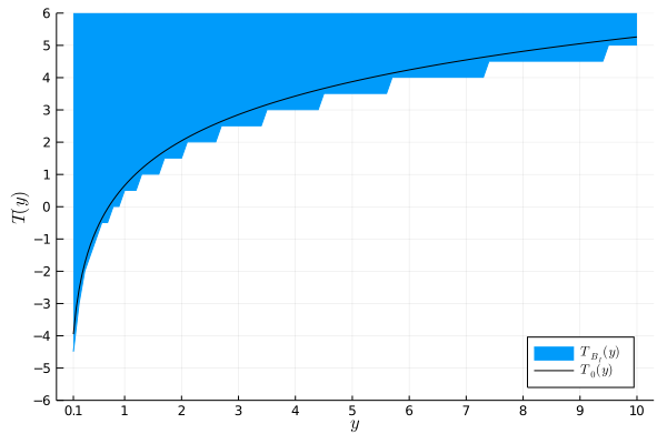
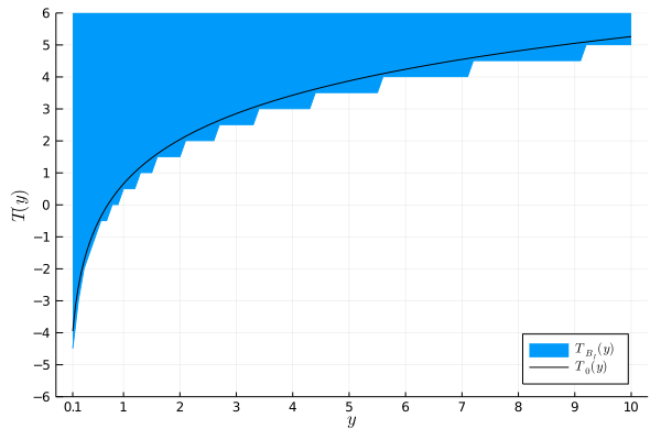
(a-1) Model 1 & Support (i) (a-2) Model 1 & Support (ii) (a-3) Model 1 & Support (iii)

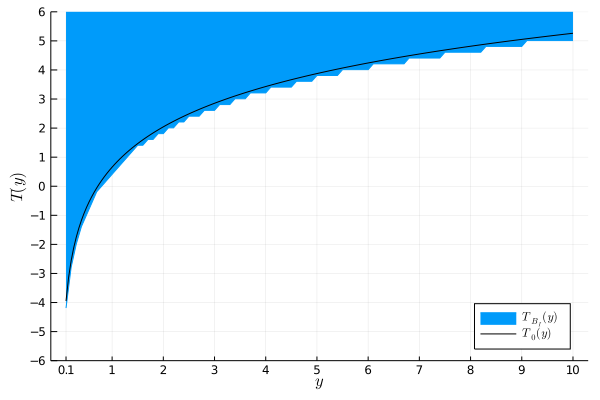
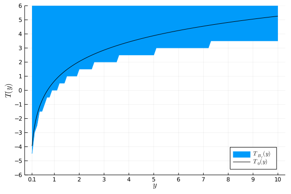
(b-1) Model 2 & Support (i) (b-2) Model 2 & Support (ii) (b-3) Model 3 & Support (iii)

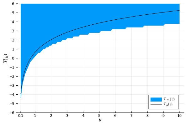
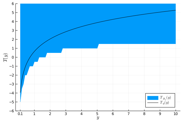
(c-1) Model 3 & Support (i) (c-2) Model 3 & Support (ii) (c-3) Model 3 & Support (iii)

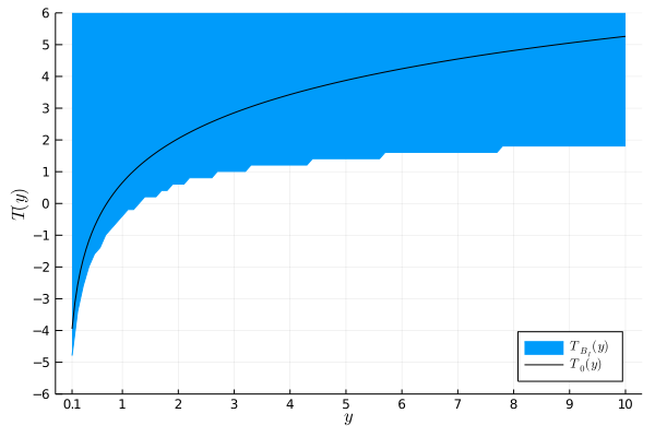
• Notes: The shaded area in each figure is the computed $T_{B_{I}}(y)$ for $0.1\leq y\leq 10$. The solid line in each figure is the graph of the true normalized transformation function $T_{0}(y)=2(\log y-\log 0.77)$.

4.2 Monte Carlo Experiments

This subsection presents Monte Carlo simulation results to evaluate the finite sample size and power properties of the inference method for the regression parameters presented in Section 3. We here use two DGPs (DGP1 and DGP2). In DGP1 and DGP2, the data are derived from Models 2 and 3, respectively, where $X_{1}$ is distributed as $N(0,2)$; $X_{2}$ is uniformly distributed over $\left\{0,1\right\}$; $U$, $V$, and $W$ have independent unit exponential distributions. The censoring rates in DGP1 and DGP2 are approximately $16\%$ and $30\%$, respectively.

For the Monte Carlo experiments, 500 samples are randomly drawn with sample sizes $n=100$, $250$, and $500$. Based on the inference method, we conduct a test of $H_{0}:$ (3.1) holds against $H_{1}:$ (3.1) is violated at each value of $\left(\beta_{1},\beta_{2}\right)\in\left\{1\right\}\times\left\{-1,-0.5,\ldots,9\right\}$. The true value of the normalized ${\beta}_{2}$ is 3. Critical values are simulated using 1,000 repetitions for the significance level $\alpha=0.05$. As a baseline case, we set the tuning parameters in the test statistics and GMS function to $R=5$, $\epsilon=0.0001$, $B_{n}=B_{n}^{bc}\equiv\left(0.8\ln\left(n\right)/\ln\ln\left(n\right)\right)^{\frac{1}{2}}$, and $\kappa_{n}=\kappa_{n}^{bc}\equiv\left(\left(1-\hat{p}_{1-D}^{1/3}\right)^{2/5}\times 0.6\ln(n)\right)^{\frac{1}{2}}$. We set $\eta=10^{-6}$ throughout this and the following sections. We do not assume that the researcher knows the exact distribution of $X_{1}$; hence, we transform $X_{1}$ into $\tilde{X}_{1}$ as described in Section 3.1 and use $\tilde{X}_{1}$ instead of $X_{1}$. We assume that the researcher knows the support of $X_{2}$. Thus we apply the inference method presented in Section 3 with $\mathcal{X}=\mathcal{X}_{1}\times\mathcal{X}_{2}=[0,1]\times\{0,1\}$.

Figure 2 shows the graphs of rejection frequencies for DGP1 and DGP2 given the baseline case of the tuning parameters with $\epsilon=0.0001$ or $\epsilon=0.001$. All the rejection frequencies at the true value of normalized $\beta_{2}$ are close to or lower than the nominal size $\alpha=0.05$ (though the rejection frequency substantially exceeds 0.05 in DGP1 with $n=100$ and $\epsilon=0.0001$). The rejection frequencies are also close to or lower than 0.05 in the corresponding intervals computed in Table 1 with Support (iii). When $\epsilon=0.001$, the test has less power but is more likely to be conservative even in small sample. The power of the test is higher at small values of $\beta_{2}$ than at large values.

Table 2 shows the rejection frequencies at the true parameter value and at $\left(\beta_{1},\beta_{2}\right)=\left(1,0\right)$ for several choices of the tuning parameters in DGP1 and DGP2. The point $\left(\beta_{1},\beta_{2}\right)=\left(1,0\right)$ is not contained in $B_{I}$, as seen from the results of the numerical examples. Table 2 shows the degree of sensitivity of the test to variation in the sample size $n$, the choice of the truncation integer $R$ in the approximate test statistic, the value of $\epsilon$ for the modified variance estimator $\bar{\sigma}_{n}^{2}\left(\beta,g\right)$, and the choice of $B_{n}$ and $\kappa_{n}$ in the GMS function. In the case of the last row of Table 2, $\kappa_{n}$ does not depend on the sample censoring rate $\hat{p}_{1-D}$. The results show that there is some sensitivity to the sample size, the choices of $\kappa_{n}$ and $R$, and the value of $\epsilon$. In particular, the sensitivity to the choice of $\kappa_{n}$ is high. A small value of $\epsilon$ leads to the test having high power, but can lead to the test having incorrect size in small samples.

The supplementary material contains two additional Monte Carlo simulation results. One examines inference on the regression parameters in models with three covariates. The other evaluates the performance of a joint inference method for the regression parameters and transformation function introduced in Appendix C.

Figure 2: Rejection Frequencies in DGP1 and DGP2

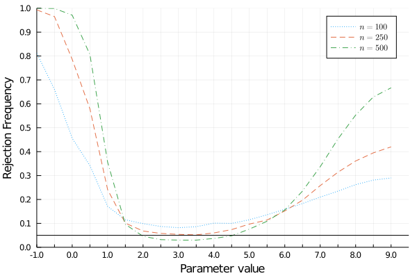
(a) DGP1 & $\epsilon=0.0001$ (b) DGP1 & $\epsilon=0.001$

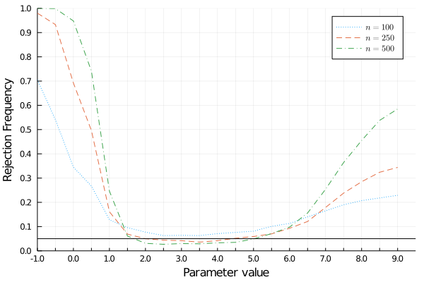
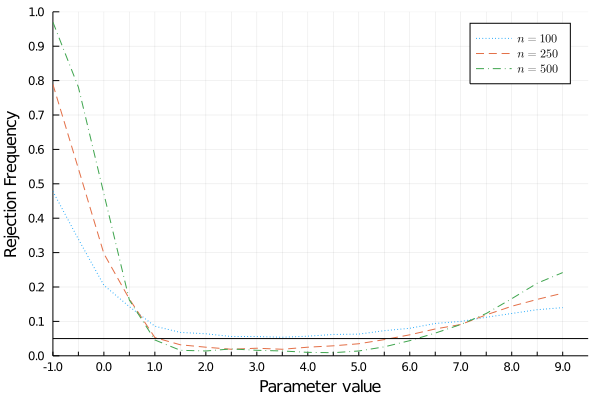
(c) DGP2 & $\epsilon=0.0001$ (d) DGP2 & $\epsilon=0.001$

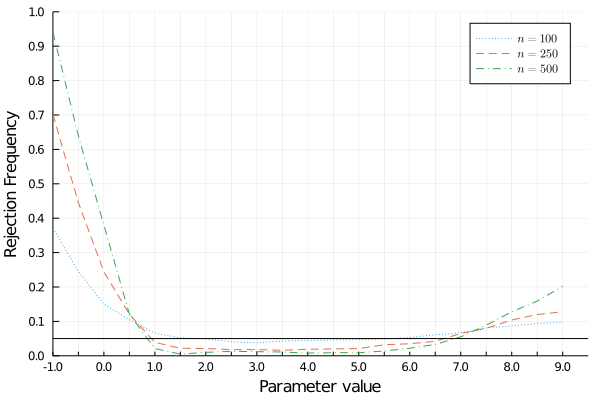
• Notes: The dashed, dotted, dash-dotted lines in each figure indicate rejection frequencies for sample sizes of $100$, $250$, and $500$, respectively. The solid horizontal line in each figure indicates the significance level of 0.05.

Table 2: Rejection Frequencies for the Inference Method: Variation in Sample Size and Choice of the Tuning Parameters

	DGP1			DGP2
Case	$\left(\beta_{1},\beta_{2}\right)=\left(1,3\right)$	$\left(\beta_{1},\beta_{2}\right)=\left(1,0\right)$		$\left(\beta_{1},\beta_{2}\right)=\left(1,3\right)$	$\left(\beta_{1},\beta_{2}\right)=\left(1,0\right)$
Baseline Case	0.054	0.786		0.022	0.297
$((n,R,B_{n},\kappa_{n},\epsilon)=(250,5,B_{n}^{bc},\kappa_{n}^{bc},0.0001))$
$\epsilon=0.001$	0.042	0.692		0.018	0.244
$\epsilon=0.00001$	0.061	0.805		0.022	0.046
$R=3$	0.052	0.594		0.046	0.192
$R=7$	0.033	0.824		0.019	0.322
$n=100,\epsilon=0.001$	0.064	0.345		0.038	0.150
$n=100,\epsilon=0.0001$	0.082	0.456		0.056	0.205
$n=100,\epsilon=0.00001$	0.089	0.489		0.058	0.227
$n=500,\epsilon=0.001$	0.030	0.948		0.012	0.380
$n=500,\epsilon=0.0001$	0.030	0.971		0.016	0.471
$n=500,\epsilon=0.00001$	0.032	0.970		0.018	0.492
$n=1000,\epsilon=0.001$	0.021	1.000		0.004	0.543
$n=1000,\epsilon=0.0001$	0.031	1.000		0.010	0.675
$n=1000,\epsilon=0.00001$	0.037	1.000		0.012	0.694
$B_{n}=B_{n}^{bc}/2$	0.053	0.786		0.021	0.297
$B_{n}=2B_{n}^{bc}$	0.054	0.786		0.022	0.297
$\kappa_{n}=\kappa_{n}^{bc}/2$	0.293	0.944		0.148	0.552
$\kappa_{n}=2\kappa_{n}^{bc}$	0.000	0.243		0.000	0.045
$\left(B_{n},\kappa_{n}\right)=1/2\left(B_{n}^{bc},\kappa_{n}^{bc}\right)$	0.288	0.944		0.140	0.550
$\left(B_{n},\kappa_{n}\right)=2\left(B_{n}^{bc},\kappa_{n}^{bc}\right)$	0.000	0.243		0.000	0.045
$\kappa_{n}=\left(0.6\ln(n)\right)^{\frac{1}{2}}$	0.026	0.683		0.010	0.217

5 Empirical Illustration

We apply the proposed inference method to evaluate the effect of heart transplants on patients’ survival duration using the Stanford Heart Transplant Data taken from Kalbfleisch and Prentice (1980). The data set consists of survival times (in days) of 103 patients; an indicator of censoring, which takes the value one if the patient is dead (uncensored) or zero if the patient is censored; an indicator of receiving a heart transplant, which takes the value one if the patient receives a heart transplant or zero otherwise; and the age (in years) of patients at the time of acceptance into the program. Among the 103 patients, $27\%$ (28 patients) are censored due to attrition or administrative censoring. The censoring rates for the treated (receive a transplant) and untreated (do not receive a transplant) groups are $35\%$ and $22\%$, respectively.

We consider the following censored transformation model,

$$T\left(Y_{0i}\right)=\min\left\{\beta_{cons}+X_{i,age}\beta_{age}+X_{i,treat}\beta_{treat}+U_{i},T\left(C_{i}\right)\right\},$$

where, for each patient $i$, $Y_{0i}$ is the observed survival time, $X_{i,age}$ is the age, $X_{i,treat}$ is the transplant indicator, $U_{i}$ is unobserved heterogeneity, $C_{i}$ is the censoring time, and $T$ is a strictly increasing function. Applying the proposed method, we allow the censoring to be arbitrarily correlated with the patient’s age and unobserved heterogeneity. Furthermore, we do not specify the transformation function or the distribution function of the patient’s unobserved heterogeneity. For scale normalization, we set $\left|\beta_{age}\right|=1$; for location normalization, we set $\beta_{cons}=0$ and $T(\tilde{y})=0$ with $\tilde{y}=90$ being the median of $Y_{0}$ in the sample. Our interest is in the normalized regression parameter $\beta_{treat}$ and the normalized transformation function $T$. We compare the proposed method with the partial rank estimator (PRE) proposed by Khan and Tamer (2007). This estimator is robust up to covariate-dependent censoring and consistently estimates the normalized regression parameters in the nonparametric transformation model.

Table 3 shows the inference results for $\beta_{treat}$. It presents the point estimate obtained from the PRE and 95% confidence intervals obtained from the PRE and the proposed method. The confidence interval obtained from the PRE is computed based on 1,000 bootstrap pseudo samples from the data. For the proposed method, we set the tuning parameters to $R=5$, $B_{n}=\left(0.8\ln\left(n\right)/\ln\ln\left(n\right)\right)^{\frac{1}{2}}$, $\kappa_{n}=\left(\left(1-\hat{p}_{1-D}^{1/3}\right)^{2/5}\times 0.6\ln(n)\right)^{\frac{1}{2}}$, and $\eta=10^{-6}$ as in the baseline case in the Monte Carlo simulation in the previous section. For $\epsilon$, we use both $\epsilon=0.0001$ and $\epsilon=0.001$. Setting $\epsilon=0.001$ is more conservative in a small sample like the Stanford Heart Transplant data set according to the Monte Carlo simulation results in the previous section. The confidence intervals obtained from the proposed method do not have finite upper bounds. This would be because age does not have sufficiently large support to derive a finite upper bound on $\beta_{treat}$ in $B_{I}$. The estimate obtained from the PRE is positive and is significantly different from zero. The 95% confidence interval obtained from the proposed method is also entirely positive regardless of the choice of $\epsilon$. With the conservative choice of $\epsilon=0.001$, the $95\%$ confidence interval obtained from the proposed method covers the confidence interval obtained from the PRE. The inference results relating to the proposed method show that even if censoring is arbitrarily correlated with a patient’s age or unobserved heterogeneity, a heart transplant has a positive effect on the patient’s survival time.

Table 3: Empirical Results for $\beta_{treat}$

	PRE	Proposed Method
		$\epsilon=0.001$	$\epsilon=0.0001$
Estimate	42.6	-	-
95% Confidence Interval	[17.2, 57.3]	[10.4, +$\infty$]	[31.3, +$\infty$]

We next apply the joint inference procedure for the regression parameters and transformation function presented in Appendix C. Figure 3 shows the marginal $95\%$-confidence set of $T(y)$ at each $y\in[0,900]$, which is the projection of the three-dimensional confidence interval of $(\beta_{age},\beta_{treat},T(y))$ on the one-dimension. The same tuning parameters as those used in Table 3 are used. Since $T_{I,\beta}(y)$ does not have a finite upper bound, neither do the confidence intervals. The estimated confidence intervals also do not have finite lower bounds for small values of $y$. The $95\%$-confidence lower bound on $T(y)$ increases rapidly with $y$ in the approximate interval $[100,250]$, but it changes slightly when $y$ is large.

Figure 3: Empirical Results for the Transformation Function

(a) $\epsilon=0.001$ (b) $\epsilon=0.0001$

• Notes: The shaded are in each figure is the computed confidence interval of $T(y)$ at each $y\in[0,900]$. The confidence intervals are computed on the range $[-10,3]$.

6 Concluding Remarks

In this paper, we propose a partial identification and inference approach for a nonparametric transformation model in the presence of endogenous censoring. We develop bounds on the regression parameters and the transformation function, each of which is characterized by conditional moment inequalities involving U-statistics. We also characterize the sharp identified set of the regression parameters, using concepts from random set theory, though this set is hard to compute. A comparison of the proposed set and the sharp identified set characterization makes it clear when the proposed set approaches the sharp set. Based on the identification result, we propose an inference method for the regression parameters by extending the inference approach for conditional moment inequality models, proposed by Andrews and Shi (2013), to the U-statistics case. We also derive the asymptotic properties of this approach. A joint inference procedure for the regression parameters and transformation function is presented in Appendix C. Numerical examples illustrate the characteristics of the proposed sets for the regression parameters and transformation function, and the results of Monte Carlo experiments demonstrate the size and power properties of the proposed inference methods. As an empirical application, we apply the inference methods to evaluate the effect of heart transplants on patients’ survival duration using data from the Stanford Heart Transplant Study, for which we find that heart transplants have a positive effect on patients’ survival duration regardless of the censoring mechanism.

Appendix

In this appendix, Section A provides proofs of Theorems 2.1 and 2.2. Section B provides a proof of Theorem 3.1 with some auxiliary lemmas. Section C presents a joint inference procedure for the regression parameters and the transformation function based on the identification results presented in Sections 2.2 and 2.4. Some additional numerical studies and Monte Carlo simulation studies are presented in the supplementary material to this paper.

Appendix A Proofs of Theorems 2.1 and 2.2

This section provides proofs of Theorems 2.1 and 2.2.

Proof of Theorem 2.1.

From the definitions of $Y_{1i}$ and $Y_{0i}$, the following holds for all $(x_{i},x_{j})\in\mathcal{X}^{2}$,

$$P(Y_{1i}\geq Y_{0j}\mid x_{i},x_{j})\geq P(Y_{i}^{\ast}\geq Y_{j}^{\ast}\mid x_{i},x_{j}).$$

For the conditional multinomial distribution $P(Y_{i}^{\ast},Y_{j}^{\ast}\mid x_{i},x_{j})$, it follows that

$$P(Y_{i}^{\ast}\geq Y_{j}^{\ast}\mid x_{i},x_{j}) =P(\Lambda(x_{i}^{\prime}\beta_{0}+U_{i})\geq\Lambda(x_{j}^{\prime}\beta_{0}+U_{j}))$$

$$\geq P(x_{i}^{\prime}\beta_{0}+U_{i}\geq x_{j}^{\prime}\beta_{0}+U_{j})$$

$$=P(U_{i}-U_{j}\geq-(x_{i}-x_{j})^{\prime}\beta_{0}).$$

The first line follows from Assumptions 2.2 and 2.3. The second line follows because $\Lambda$ is a monotonically increasing function by Assumption 2.1. When $(x_{i}-x_{j})^{\prime}\beta_{0}\geq 0$,

$$P(U_{i}-U_{j}\geq-(x_{i}-x_{j})^{\prime}\beta_{0})\geq\frac{1}{2}$$

holds because $U_{i}-U_{j}$ is symmetrically distributed about zero under Assumption 2.2. Therefore it follows that

$$x_{i}^{\prime}\beta_{0}\geq x_{j}^{\prime}\beta_{0} \Rightarrow P\left(Y_{i}^{\ast}\geq Y_{j}^{\ast}\mid x_{i},x_{j}\right)\geq\frac{1}{2}$$

$$\Rightarrow P(Y_{1i}\geq Y_{0j}\mid x_{i},x_{j})\geq\frac{1}{2}$$

for all $(x_{i},x_{j})\in\mathcal{X}^{2}$. This implies that $\beta_{0}\in B_{I}$ a.s..

We next show that $B_{I}$ is a proper subset of $B$. Let $(\tilde{x}_{i},\tilde{x}_{j})\in\widetilde{\mathcal{X}}^{2}$. Then there exist $\beta\in B$ such that

$$\tilde{x}_{i}^{\prime}\beta\geq\tilde{x}_{j}^{\prime}\beta\Rightarrow P(Y_{1i}\geq Y_{0j}\mid\tilde{x}_{i},\tilde{x}_{j})<\frac{1}{2}.$$

Such a $\beta$ is not a member of $B_{I}$. Hence, because $P((X_{i},X_{j})\in\widetilde{\mathcal{X}}^{2})>0$ by Assumption 2.4, $B_{I}\subset B$ holds a.s. ∎

Proof of Theorem 2.2.

Under Assumptions 2.2, 2.3, and 2.5, $\beta_{0}\in B_{I}$ a.s. from Theorem 2.1. Then it suffices to show that $T\left(y\right)\in T_{I,\beta_{0}}\left(y\right)$ a.s. for any $y\in\mathbb{R}$.

Let $y\in\mathbb{R}$ be fixed. Note that from the definitions of $Y_{1i}$ and $Y_{0i}$,

$$P(Y_{1i}\geq y\mid x_{i})-P(Y_{0j}\geq\tilde{y}\mid x_{j})\geq P(Y_{i}^{\ast}\geq y\mid x_{i})-P(Y_{j}^{\ast}\geq\tilde{y}\mid x_{j}).$$

holds for all $(x_{i},x_{j})\in\mathcal{X}^{2}$.

For the conditional multinomial distribution $P(Y_{i}^{\ast},Y_{j}^{\ast}\mid x_{i},x_{j})$, it follows that

$$P(Y_{i}^{\ast}\geq y\mid x_{i})-P(Y_{j}^{\ast}\geq\tilde{y}\mid x_{j})$$

$$= \ P\left(x_{i}^{\prime}\beta_{0}+U_{i}\geq T\left(y\right)\mid x_{i}\right)-P\left(x_{j}^{\prime}\beta_{0}+U_{j}\geq 0\mid x_{j}\right)$$

$$= \ F_{U}\left(-x_{j}^{\prime}\beta_{0}\right)-F_{U}\left(T\left(y\right)-x_{i}^{\prime}\beta_{0}\right).$$

The first equality follows from Assumptions 2.2 and 2.5 and the fact that $T\left(\tilde{y}\right)=0$ for the location normalization. The second equality follows from Assumptions 2.2 and 2.3. Since

$$x_{i}^{\prime}\beta_{0}-x_{j}^{\prime}\beta_{0}\geq T\left(y\right)\Rightarrow F_{U}\left(-x_{j}^{\prime}\beta_{0}\right)\geq F_{U}\left(T\left(y\right)-x_{i}^{\prime}\beta_{0}\right),$$

we have

$$x_{i}^{\prime}\beta_{0}-x_{j}^{\prime}\beta_{0}\geq T\left(y\right) \Rightarrow P(Y_{i}^{\ast}\geq y\mid x_{i})-P(Y_{j}^{\ast}\geq\tilde{y}\mid x_{j})\geq 0$$

$$\Rightarrow P(Y_{1i}\geq y\mid x_{i})-P(Y_{0j}\geq\tilde{y}\mid x_{j})\geq 0$$

for all $(x_{i},x_{j})\in\mathcal{X}^{2}$. This implies that $T\left(y\right)\in T_{I,\beta_{0}}\left(y\right)$ a.s. ∎

Appendix B Proof of Theorem 3.1

This section provides a proof of the uniform asymptotic probability results for the inference method presented in Section 3. The outline of the proof is same as that of the proofs of Theorems 2(b) and 3 in AS, but we modify them for the case of U-statistics. Let $\rightsquigarrow$ denote weak convergence of a stochastic process in the sense of Pollard (1990). The following notations are similar to the notations introduced in AS,

$$v_{n,P}\left(\beta,g\right)\equiv n^{\frac{1}{2}}\left(\bar{m}_{n}\left(\beta,g\right)-E_{P}\left[m(W_{i},W_{j},\beta,g)\right]\right)/\sigma_{p}\left(\beta\right)$$

and

$$\hat{h}_{2,n,P}\left(\beta,g,g^{\ast}\right)\equiv \left\{\frac{1}{n\left(n-1\right)\left(n-2\right)}\sum_{i\neq j\neq k}m(W_{i},W_{j},\beta,g)m(W_{i},W_{k},\beta,g^{\ast})\right.$$

$$\left.-E_{P}\left[m(W_{i},W_{j},\beta,g)\right]\cdot E_{P}\left[m\left(W_{i},W_{j},\beta,g^{\ast}\right)\right]\right\}/\sigma_{P}^{2}\left(\beta\right).$$

Let $\left\{v_{h_{2}}\left(g\right):g\in{\cal G}\right\}$ be a mean zero Gaussian process with some covariance kernel $h_{2}\left(\cdot,\cdot\right)$ on ${\cal G}\times{\cal G}$. Let $\{a_{n}:n\geq 1\}$ denote a subsequence of $\{n\}$.

To prove Theorem 3.1, we first prove that the following two lemmas hold. Lemma B.1 implies that Assumption EP in AS holds. Lemmas B.2 implies that a version of Assumption CI in AS, which is modified for the case of U-statistics, holds.

Lemma B.1.

For any subsequence $\left\{\left(\beta_{a_{n}},P_{a_{n}}\right)\in{\cal Q}:n\geq 1\right\}$ such that

$$\underset{n\rightarrow\infty}{\lim}\underset{g,g^{\ast}\in{\cal G}}{\sup}\left\|h_{2,P_{a_{n}}}\left(\beta_{a_{n}},g,g^{\ast}\right)-h_{2}\left(g,g^{\ast}\right)\right\|=0$$

for some covariance kernel $h_{2}(\cdot,\cdot)$ on ${\cal G}\times{\cal G}$, we have
(a) $\sqrt{a_{n}}v_{a_{n},P_{a_{n}}}\left(\beta_{a_{n}},\cdot\right)\rightsquigarrow v_{h_{2}}\left(\cdot\right)$ as $n\rightarrow\infty$, and
(b) $\underset{\left(g,g^{\ast}\right)\in{\cal G}\times\mathcal{G}}{\sup}\left\|\hat{h}_{2,a_{n},P_{a_{n}}}\left(\beta_{a_{n}},g,g^{\ast}\right)-h_{2}\left(g,g^{\ast}\right)\right\|\underset{p}{\rightarrow}0$ as $n\rightarrow\infty$.

Lemma B.2.

For any $\beta\in B$ and any distribution function $P$ that satisfies Assumptions 2.1–2.3, let

$${\cal X}_{P}\left(\beta\right)=\left\{(x_{i},x_{j})\in{\cal X}^{2}:E_{P}\left[m\left(W_{i},W_{j},\beta\right)\mid x_{i},x_{j}\right]<0\right\}.$$

Then, for any $\beta\in B$ and $P$ that satisfies Assumptions 2.1–2.3 and $P\left((x_{i},x_{j})\in{\cal X}_{P}\left(\beta\right)\right)>0,$ there exists some $g\in{\cal G}$ such that

$$E_{P}\left[m(W_{i},W_{j},\beta,g)\right]<0.$$

The next lemma with a proof is auxiliary to Lemma B.1.

Lemma B.3.

Let $(\beta,P)\in\mathcal{{Q}}$. Define classes of functions ${\cal F}_{1}=\left\{f_{1}(\cdot,\cdot,\beta,g):g\in{\cal G}\right\}$ and ${\cal F}_{2}=\left\{f_{2}(\cdot,\cdot,\cdot,\beta,g,g^{\ast}):\left(g,g^{\ast}\right)\in{\cal G}\times{\cal G}\right\}$, where

$$f_{1}(w_{i},w_{j},\beta,g)=m(w_{i},w_{j},\beta,g)-E_{P}\left[m(W_{i},W_{j},\beta,g)\right]$$

and

$$f_{2}(w_{i},w_{j},w_{k},\beta,g,g^{\ast})= \ m(w_{i},w_{j},\beta,g)\cdot m(w_{i},w_{k},\beta,g^{\ast})$$

$$-E_{P}\left[m(W_{i},W_{j},\beta,g)\right]\cdot E_{P}\left[m\left(W_{i},W_{j},\beta,g^{\ast}\right)\right].$$

Then $\mathcal{F}_{1}$ and $\mathcal{F}_{2}$ are Euclidean classes of functions for constant envelopes $1$ and $1/2$, respectively, in the sense of Nolan and Pollard (1987).

Proof of Lemma B.3.

We consider the class of function $\mathcal{G}$ defined in Section 3.1. For any $x\in\mathbb{R}^{k}$, let $x=(x^{(1)\prime},x^{(2)\prime})$ where $x^{(1)}$ is a vector of the first $p$ elements of $x$ and $x^{(2)}$ is a vector of the remaining $k-p$ elements of $x$. $\mathcal{G}$ is represented as

$$\mathcal{G}= \left\{I\left[\frac{a-\mathbf{1}_{p}}{2r}<x_{i}^{(1)}\leq\frac{a}{2r},x_{i}^{(2)}=b\right]\cdot I\left[\frac{\tilde{a}-\mathbf{1}_{p}}{2r}<x_{j}^{(1)}\leq\frac{\tilde{a}}{2r},x_{j}^{(2)}=\tilde{b}\right]:\right.$$

$$a=(a_{1},\ldots,a_{p})^{\prime},\ \tilde{a}=\left(\tilde{a}_{1},\ldots,\tilde{a}_{p}\right)^{\prime},\ \left(a_{u},\tilde{a}_{u}\right)\in\left\{1,2,\ldots,2r\right\}^{2}$$

$$\left.\mbox{for }u=1,\ldots,p\ \mbox{and }r=1,2,\ldots,\mbox{ and }(b,\tilde{b})\in\mathcal{X}_{2}^{2}\right\},$$

where $\mathbf{1}_{p}$ is a $p$-dimensional vector of ones. Because the collection of cells in $\mathbb{R}^{2k}$ is a Vapnik-Chervonenkis (VC) class of sets (see van der Vaart and Wellner (1996, Example 2.6.1)), the collection of all subgraphs, $\left\{\left(x_{i},x_{j},t\right):t<g(x_{i},x_{j})\right\}$, of the function in $\mathcal{G}$ forms a VC class of sets in $\mathcal{X}^{2}\times\mathbb{R}$. Hence, $\mathcal{G}$ is a VC class of functions. Combining this result with Lemma 2.6.18 in van der Vaart and Wellner (1996), $\mathcal{F}_{1}$ and $\mathcal{F}_{2}$ are VC-classes of functions. Thus, from Corollary 19 in Nolan and Pollard (1987), $\mathcal{F}_{1}$ and $\mathcal{F}_{2}$ are Euclidean classes of functions. $\mathcal{F}_{1}$ and $\mathcal{F}_{2}$ obviously have the constant envelopes $1$ and $1/2$, respectively, from their definitions. ∎

We provide proofs of Lemmas B.1 and B.2 and Theorem 3.1 below.

Proof of Lemma B.1.(a).

While Lemma B.1 is stated in terms of a subsequence $\left\{a_{n}\right\}$, for notational simplicity, we prove it for the sequence $\left\{n\right\}$. All of the arguments in this and the next proofs proceed with $\left\{a_{n}\right\}$ instead of $\left\{n\right\}$.

We use Theorem 5 in Nolan and Pollard (1988) to show that the weak convergence result in Lemma B.1.(a) holds. Let $(\beta,P)$ be the limit of $(\beta_{n},P_{n})$ and $h_{2}(\cdot,\cdot)=h_{2,P}(\beta,\cdot,\cdot)$. Let $N_{p}\left(\epsilon,Q,{\cal F},F\right)$ denote the $L_{p}\left(Q\right)$-covering number of radius $\epsilon$ for a functional space ${\cal F}$ with a envelope function $F$ where $Q$ is some probability measure on $\mathcal{X}$. For any distribution $Q$ on $\mathcal{X}$, let $Q{\cal F}_{1}\equiv\{Qf_{1}(x,\cdot,\beta,g):g\in\mathcal{G}\}$ be the class of functions $Qf_{1}\left(x,\cdot,\beta,g\right)$ on ${\cal X}$, where $f_{1}$ and $\mathcal{F}_{1}$ are defined in Lemma B.3 and $Qf_{1}(x,\cdot,\beta,g)\equiv\int_{\mathcal{X}}f_{1}(x,x_{2},\beta,g)dQ_{X}(x_{2})$.

To apply Theorem 5 in Nolan and Pollard (1988), it suffices to show that the following conditions hold:

(i)

$\sup_{Q}\intop_{0}^{1}\log N_{2}\left(\epsilon,Q\times Q,{\cal F}_{1},F\right)d\epsilon<\infty$, $\sup_{Q}\left(\intop_{0}^{1}\log N_{2}\left(\epsilon,Q\times Q,\mathcal{F}_{1},F\right)d\epsilon\right)^{2}<\infty$, and $\sup_{Q}\left(\intop_{0}^{1}\log N_{2}\left(\epsilon,Q,P\mathcal{F}_{1},PF\right)d\epsilon\right)^{2}<\infty$;

(ii)

as $\gamma\searrow 0$,

$$\sup_{Q}\intop_{0}^{\gamma}\log N_{2}\left(\epsilon,Q,P{\cal F}_{1},PF\right)\rightarrow 0,$$

where $Q$ is any probability measure on $\mathcal{X}$. We show below that these two conditions are satisfied.

We first consider condition (i). From Lemma B.3, the class of functions $\mathcal{F}_{1}$ is Euclidean with the constant envelope $F=1$. Then, from Corollary 21 in Nolan and Pollard (1987), the class of functions $P{\cal F}_{1}$ is also a Euclidean class with the constant envelope $1$. From page 789 in Nolan and Pollard (1987), if a Euclidean class has a constant envelope function, then the upper bound on the $L_{p}(Q)$-covering number of radius $\epsilon$ for it is uniform in any probability measure $Q$ on $\mathcal{X}$. Therefore, since $\mathcal{F}_{1}$ and $P{\cal F}_{1}$ are Euclidean classes with constant envelopes, for any $0<\epsilon\leq 1$, there exist some constants $K_{2}$, $K_{2}^{\ast}$, $V_{2}$, and $V_{2}^{\ast}$ such that $N_{2}\left(\epsilon,Q\times Q,{\cal F}_{1},F\right)\leq K_{2}\epsilon^{-2V_{2}}$ and $N_{2}\left(\epsilon,Q,P{\cal F}_{1},PF\right)\leq K_{2}^{\ast}\epsilon^{-2V_{2}^{\ast}}$, for any probability measure $Q$ on $\mathcal{X}$. Then it follows that

$$\sup_{Q}\intop_{0}^{1}\log N_{2}\left(\epsilon,Q\times Q,{\cal F}_{1},F\right)d\epsilon \leq\intop_{0}^{1}\left(\log K_{2}\epsilon^{-2V_{2}}\right)d\epsilon<\infty,$$

$$\sup_{Q}\left(\intop_{0}^{1}\log N_{2}\left(\epsilon,Q\times Q,{\cal F}_{1},F\right)d\epsilon\right)^{2} \leq\left(\intop_{0}^{1}\left(\log K_{2}\epsilon^{-2V_{2}}\right)d\epsilon\right)^{2}<\infty,$$

and

$$\sup_{Q}\left(\intop_{0}^{1}\log N_{2}\left(\epsilon,Q,P{\cal F}_{1},PF\right)d\epsilon\right)^{2}\leq\left(\intop_{0}^{1}\left(\log K_{2}^{\ast}\epsilon^{-2V_{2}^{\ast}}\right)d\epsilon\right)^{2}<\infty.$$

These imply that condition (i) is satisfied.

Next, as $\gamma\searrow 0$,

$$\sup_{Q}\intop_{0}^{\gamma}\log N_{2}\left(\epsilon,Q,P{\cal F}_{1},PF\right)d\epsilon \leq\intop_{0}^{\gamma}\log(K_{2}^{\ast}\epsilon^{-2V_{2}^{\ast}})d\epsilon$$

$$=\gamma\log K_{2}^{\ast}-2V_{2}^{\ast}\gamma(\log\gamma-1)$$

$$\rightarrow 0.$$

This implies that condition (ii) is satisfied. Therefore, from Theorem 5 in Nolan and Pollard (1988) and the fact that $\beta_{n}\rightarrow\beta$ and $\sigma_{P_{n}}\left(\beta_{n}\right)\underset{p}{\rightarrow}\sigma_{P}\left(\beta\right)$, Lemma B.1.(a) holds by the extended continuous mapping theorem (Theorem 1.11.1 in van der Vaart and Wellner (1996)). ∎

Proof of Lemma B.1.(b).

Let $(\beta,P)$ be the limit of $(\beta_{n},P_{n})$. Since $\mathcal{F}_{1}$ and $\mathcal{F}_{2}$ are Euclidean classes with constant envelopes from Lemma B.3, by applying Corollary 7 in Sherman (1994), it follows that

$$\sup_{g\in{\cal G}}\left\|\frac{1}{n\left(n-1\right)}\sum_{i\neq j}f_{1}(W_{i},W_{j},\beta,g)\right\|\underset{p}{\rightarrow}0$$

and

$$\sup_{(g,g^{*})\in\mathcal{G}\times\mathcal{G}}\left\|\frac{1}{n\left(n-1\right)\left(n-2\right)}\sum_{i\neq j\neq k}f_{2}(W_{i},W_{j},W_{k},\beta,g,g^{\ast})\right\|\underset{p}{\rightarrow}0.$$

Therefore, letting $h_{2}\left(\beta,g,g^{\ast}\right)=h_{2,P}\left(\beta,g,g^{\ast}\right)$ be given by (3.2) and further dividing by $\sigma_{P}^{2}\left(\beta\right)$, as $\beta_{n}\rightarrow\beta$ and $\sigma_{P_{n}}\left(\beta_{n}\right)\underset{p}{\rightarrow}\sigma_{P}\left(\beta\right)$, we have

$$\ \underset{(g,g^{\ast})\in\mathcal{G}\times\mathcal{G}}{\sup}\left\|\hat{h}_{2,a_{n},P_{n}}\left(\beta_{n},g,g^{\ast}\right)-h_{2}\left(\beta,g,g^{\ast}\right)\right\|$$

$$\leq \ \sup_{(g,g^{\ast})\in\mathcal{G}\times\mathcal{G}}\left\|\frac{1}{n\left(n-1\right)\left(n-2\right)}\sum_{i\neq j\neq k}f_{2}(W_{i},W_{j},W_{k},\beta,g,g^{\ast})/\sigma_{P}\left(\beta\right)\right\|$$

$$\ +\left\{\sup_{g\in{\cal G}}\left\|\frac{1}{n\left(n-1\right)\left(n-2\right)}\sum_{i\neq j}f_{1}(W_{i},W_{j},\beta,g)/\sigma_{P}\left(\beta\right)\right\|\right\}^{2}+o_{p}\left(1\right)$$

$$\underset{p}{\rightarrow} \ 0.$$

∎

Proof of Lemma B.2.

It suffices to show that

$$E_{P}\left[m(W_{i},W_{j},\beta,g)\right]\geq 0\ \ \forall g\in{\cal G}$$

$$\Rightarrow\ E_{P}\left[m\left(W_{i},W_{j},\beta\right)\mid x_{i},x_{j}\right]\geq 0\ \ \mbox{for almost every $(x_{i},x_{j})\in\mathcal{X}^{2}$.}$$ (B.1)

Let $X=(X^{(1)\prime},X^{(2)\prime})^{\prime}$ where $X^{(1)}$ and $X^{(2)}$ are distributed on $\mathcal{X}_{1}$ and $\mathcal{X}_{2}$, respectively. Let $(b,\tilde{b})\in\mathcal{X}_{2}^{2}$ be fixed, and define a class of instrumental functions

$$\widetilde{\mathcal{G}}=\left\{g\left(x_{i}^{(1)},x_{j}^{(1)}\right)=I\left[\left(x_{i}^{(1)},x_{j}^{(1)}\right)\in J_{1}\right]\ \mbox{for}\ J_{1}\in\mathcal{J}_{1}\right\},$$

where

$$\mathcal{J}_{1}\equiv \left\{J_{(a,\tilde{a},r)}=\left(\vartimes_{u=1}^{p}\left(\frac{a_{u}-1}{2r},\frac{a_{u}}{2r}\right]\right)\times\left(\vartimes_{u=1}^{p}\left(\frac{\tilde{a}_{u}-1}{2r},\frac{\tilde{a}_{u}}{2r}\right]\right):\right.$$

$$\ \left.a=(a_{1},\ldots,a_{p}),\ \tilde{a}=(\tilde{a}_{1},\ldots,\tilde{a}_{p}),\ a_{u}\in\left\{1,2,\ldots,2r\right\},\ \tilde{a}_{u}\in\left\{1,2,\ldots,2r\right\}\right.$$

$$\ \left.\mbox{for}\ u=1,\ldots,p\ \mbox{and}\ r=1,2,\ldots\right\}.$$

Then, to prove (B.1), it suffices to show that

$$E_{P}\left[m(W_{i},W_{j},\beta,g)\mid(X_{i}^{(2)},X_{j}^{(2)})=(b,\tilde{b})\right]\geq 0\ \ \forall g\in\widetilde{\mathcal{G}}$$

$$\Rightarrow\ E_{P}\left[m\left(W_{i},W_{j},\beta\right)\mid(X_{i}^{(1)},X_{j}^{(1)})=(x_{i}^{(1)},x_{j}^{(1)}),(X_{i}^{(2)},X_{j}^{(2)})=(b,\tilde{b})\right]\geq 0$$

$$\mbox{ for almost every $(x_{i}^{(1)},x_{j}^{(1)})\in\mathcal{X}_{1}^{2}$}.$$ (B.2)

We invoke Lemma C1 in AS. Let ${\cal R}$ be a semiring of subsets of $\mathbb{R}^{2p}$ and

$$\mu(J_{1})\equiv E_{P}\left[m\left(W_{i},W_{j},\beta\right)\cdot I\left[\left(X_{i}^{(1)},X_{j}^{(1)}\right)\in J_{1}\right]\mid(X_{i}^{(2)},X_{j}^{(2)})=(b,\tilde{b})\right]$$

for $J_{1}\in\sigma\left(\mathcal{J}_{1}\right)={\cal B}\left(\mathbb{R}^{2p}\right)$, where $\sigma\left(\mathcal{J}_{1}\right)$ denotes the $\sigma$-field generated by $\mathcal{J}_{1}$ and ${\cal B}\left(\mathbb{R}^{2p}\right)$ is the Borel $\sigma$-field on $\mathbb{R}^{2p}$. $\sigma\left(\mathcal{J}_{1}\right)={\cal B}\left(\mathbb{R}^{2p}\right)$ is a well known result. We show that all conditions of Lemma C1 in AS are satisfied. Then condition (B.2) holds from Lemma C1 in AS.

First, $\mathcal{J}_{1}$ is a semiring of subsets of $\mathbb{R}^{2p}$. Since $m\left(W_{i},W_{j},\beta\right)$ and $I\left[\left(X_{i}^{(1)},X_{j}^{(1)}\right)\in J_{1}\right]$ are bounded functions, $\mu(\cdot)$ satisfies the boundedness condition of Lemma C1 in AS. The other conditions of Lemma C1 in AS also hold by the same argument as the proof of Lemma 3 in AS. Thus, by applying Lemma C1 in AS, the fact that $\mu(J_{1})\geq 0$ for all $J_{1}\in\mathcal{J}_{1}$ implies that $E_{P}\left[m\left(W_{i},W_{j},\beta\right)\cdot I\left[\left(X_{i}^{(1)},X_{j}^{(1)}\right)\in J_{1}\mid(X_{i}^{(2)},X_{j}^{(2)})=(b,\tilde{b})\right]\right]\geq 0$ for all $J_{1}\in\sigma(\mathcal{J}_{1})$, which is equivalent to ${\cal B}\left(\mathbb{R}^{2p}\right)$. This implies that the result of Lemma B.2 holds. ∎

Let $Q$ be a measure on $\mathcal{G}$ such that, for $g_{(a,b),(\tilde{a},\tilde{b}),r}\in\mathcal{G}$,

$$Q(g_{(a,b),(\tilde{a},\tilde{b}),r})=(r^{2}+100)^{-1}\cdot((2r)^{p}\cdot|\mathcal{X}_{2}|)^{-2}.$$

Then $T_{n}(\beta)$ is expressed as

$$T_{n}(\beta)=\int_{g\in\mathcal{G}}S(n^{\frac{1}{2}}\bar{m}_{n}(\beta,g),\bar{\sigma}_{n}(\beta,g))dQ(g),$$ (B.3)

where $S(m,\sigma)\equiv[m/\sigma]_{-}^{2}$.

The following lemma shows that $Q$ satisfies Assumption Q in AS.

Lemma B.4.

Suppose that Assumption 2.2 holds. Define the pseud-metric $\rho_{X}$ on $\mathcal{G}$ by

$$\rho_{X}(g,g^{\ast})\equiv(E_{P_{X}}[|g(X_{i},X_{j})-g^{\ast}(X_{i},X_{j})|])^{1/2}\mbox{ for }(g,g^{*})\in\mathcal{G}\times\mathcal{G},$$

where $E_{P_{X}}[\cdot]$ denotes the expectation under $X\sim P_{X}$. Let $\mathcal{B}_{\rho_{X}}(g,\delta)$ denote an open $\rho_{X}$-ball in $\mathcal{G}$ centered at $g$ with radius $\delta$. Then the support of $Q$ under $\rho_{X}$ is $\mathcal{G}$. That is, for all $\delta>0$, $Q(\mathcal{B}_{\rho_{X}}(g,\delta))>0$ for all $g\in\mathcal{G}$.

Proof.

We prove the statement in the case of $p=k$. Then the result for the other case $p<k$ immediately follows. Let $AR\equiv\{(a,\tilde{a},r):(a,\tilde{a})\in\{1,\ldots,2r\}^{2k}\mbox{ and }r=1,2,\ldots\}$. Then there is a one-to-one mapping $\Pi:\mathcal{G}\rightarrow AR$. The weight function $Q$ can be expressed as $Q=\Pi^{-1}Q_{AR}$, where $Q_{AR}$ is a measure on $2^{AR}$ such that $Q((a,\tilde{a},r))=(r^{2}+100)^{-1}\cdot(2r)^{-2k}$ for any $(a,\tilde{a},r)\in AR$. Then the statement follows by applying Lemma 4 in AS to $Q=\Pi^{-1}Q_{AR}$. ∎

Proof of Theorem 3.1.

To show that Theorem 3.1 holds, it suffices to show that all required conditions in Theorems 2(b) and 3 in AS are satisfied. We first check that the functions $S$ and $Q$ in (B.3) satisfy the required conditions. Since the function $S$ corresponds to the modified method moments function in AS (Equation (3.8) in AS), Lemma 1 in AS guarantees that the function $S$ in (B.3) satisfies Assumptions S1–4 in AS. Lemma B.4 shows that the weight function $Q$ in (B.3) satisfies Assumption Q in AS. Lemma B.1 implies that Assumption EP in AS holds. Then Lemma B3 in AS guarantees that Assumption GMS2(a) in AS holds. Assumption 3.1 implies that the tuning parameters in the GMS function satisfy Assumptions GMS1, GMS2(b), and GMS2(c) in AS. Therefore, Theorem 3.1(a) follows from Theorem 2(b) in AS.

For result (b), Lemma B.2 in this appendix has the same role as Assumption CI in AS. The assumption $P((X_{i},X_{j})\in\mathcal{X}_{P}^{2}(\tilde{\beta}))>0$ in Theorem 3.1(b) corresponds to Assumption FA(a) in AS. Note that Lemma B.1 applies for $(\beta_{a_{n}},P_{a_{n}})=(\tilde{\beta},P)$ by the same argument as in the proof of Lemma B.1. Therefore, by the same arguments as in Section 14.2 in AS, where we replace Lemma A1 (in AS) for $(\beta_{a_{n}},P_{a_{n}})=(\tilde{\beta},P)$ by Lemma B.1 for $(\beta_{a_{n}},P_{a_{n}})=(\tilde{\beta},P)$, Theorem 3.1(b) holds. ∎

Appendix C Inference for the Transformation Function

This section provides a joint inference procedure for $\beta_{0}$ and $\{T\left(y\right)\}_{y\in\mathbf{y}}$, where $\mathbf{y}$ is a finite set of $y$. Let $q$ be the dimension of $\mathbf{y}$ and denote $\mathbf{y}=(y_{1},\ldots,y_{q})^{\prime}$. We first note that with fixed $y\in\mathbb{R}$ and $\beta$, $T_{I,\beta}(y)$ is equivalent to the set of all values $t\in\mathbb{R}$ that satisfy the following conditional moment inequality condition:

$$E_{P}\left[m^{\dagger}(W_{i},W_{j},\beta,y,t)\mid x_{i},x_{j}\right]\geq 0\mbox{ for all $(x_{i},x_{j})\in\mathcal{X}^{2}$},$$ (C.1)

where $m^{\dagger}(W_{i},W_{j},\beta,y,t)$ is a moment function defined as

$$m^{\dagger}\left(W_{i},W_{j},\beta,y,t\right) \equiv\left(I\left[Y_{1i}\geq y\right]-I\left[Y_{0j}\geq\tilde{y}\right]\right)\cdot I[X_{i}^{\prime}\beta-X_{j}^{\prime}\beta\geq t]$$

$$+\left(I\left[Y_{1j}\geq y\right]-I\left[Y_{0i}\geq\tilde{y}\right]\right)\cdot I[X_{j}^{\prime}\beta-X_{i}^{\prime}\beta\geq t].$$

This is obvious from the definition of $T_{I,\beta}(y)$. The joint inference procedure for $\beta_{0}$ and $\{T\left(y\right)\}_{y\in\mathbf{y}}$ is then constructed by applying the conditional moment inequality inference approach presented in Section 3 to the conditional moment inequalities (3.1) and (C.1).

Fix $y\in\mathbf{y}$. Let $m^{\dagger}\left(W_{i},W_{j},\beta,y,t,g\right)\equiv m^{\dagger}\left(W_{i},W_{j},\beta,y,t\right)\cdot g(x_{i},x_{j})$ for any $g\in\mathcal{G}$, where $\mathcal{G}$ is the set of instrumental functions defined in Section 3.1. Then $T_{I,\beta}\left(y\right)$ is equivalent to

$$\left\{t\in\mathbb{R}:\ E_{P}\left[m^{\dagger}\left(W_{i},W_{j},\beta,y,t,g\right)\right]\geq 0\ \mbox{for all}\ g\in\mathcal{G}\right\}.$$

Define the sample moment function and sample variance function, respectively, by

$$\bar{m}_{n}^{\dagger}\left(\beta,y,t,g\right)\equiv\frac{1}{n\left(n-1\right)}\sum_{i\neq j}m^{\dagger}\left(W_{i},W_{j},\beta,y,t,g\right)$$

and

$$\hat{\sigma}_{n}^{\dagger 2}\left(\beta,y,t,g\right)\equiv \left\{\frac{1}{n\left(n-1\right)\left(n-2\right)}\sum_{i\neq j\neq k}m^{\dagger}\left(W_{i},W_{j},\beta,y,t,g\right)m^{\dagger}\left(W_{i},W_{k},\beta,y,t,g\right)\right.$$

$$\left.-\left(\frac{1}{n(n-1)}\sum_{i\neq j}m^{\dagger}\left(W_{i},W_{j},\beta,y,t,g\right)\right)^{2}\right\}.$$

Since the function $\bar{m}_{n}^{\dagger}\left(\beta,y,t,g\right)$ is a U-statistic of order two, the estimator of its asymptotic variance, $\hat{\sigma}_{n}^{\dagger 2}\left(\beta,y,t,g\right)$, is constructed with a similar form to $\hat{\sigma}_{n}^{2}\left(\beta,g\right)$ in Section 3.1. In practice, we use the modified sample variance function:

$$\bar{\sigma}_{n}^{\dagger 2}\left(\beta,y,t,g\right)\equiv\hat{\sigma}_{n}^{\dagger 2}\left(\beta,y,t,g\right)+\epsilon\hat{\sigma}_{n}^{\dagger 2}(y),$$

where $\hat{\sigma}_{n}^{\dagger 2}(y)\equiv\hat{\sigma}_{n}^{\dagger 2}\left(\beta,y,t,1\right)$ and $\epsilon$ is the regularization parameter (e.g., $\epsilon=0.0001$).

Then, for any $\beta\in B$ and $\mathbf{t}=(t_{1},\ldots,t_{q})^{\prime}\in\mathbb{R}^{q}$, an approximate test statistic for a null hypothesis:

$$H_{0}: \ E_{P}\left[m(W_{i},W_{j},\beta)\mid x_{i},x_{j}\right]\geq 0\mbox{ and }E_{P}\left[m^{\dagger}(W_{i},W_{j},\beta,y_{\ell},t_{\ell})\mid x_{i},x_{j}\right]\geq 0$$

$$\mbox{for all }\ell=1,\ldots,q\mbox{ and }(x_{i},x_{j})\in\mathcal{X}^{2}$$

is constructed as

$$T_{\mathbf{y},n,R}^{\dagger}(\beta,\mathbf{t})\equiv \ \sum_{r=1}^{R}\left(r^{2}+100\right)^{-1}\sum_{\left(a,\tilde{a}\right)\in\left\{1,\cdots,2r\right\}^{2p}}\sum_{(b,\tilde{b})\in\mathcal{X}_{2}^{2}}\frac{1}{(2r)^{2p}\cdot|\mathcal{X}_{2}|^{2}}\left(\left[\frac{n^{\frac{1}{2}}\bar{m}_{n}\left(\beta,g_{(a,b),(\tilde{a},\tilde{b}),r}\right)}{\bar{\sigma}_{n}\left(\beta,g_{(a,b),(\tilde{a},\tilde{b}),r}\right)}\right]_{-}^{2}\right.$$

$$\left.+\sum_{j=1}^{q}\left[\frac{n^{\frac{1}{2}}\bar{m}_{n}^{\dagger}\left(\beta,y_{j},t_{j},g_{(a,b),(\tilde{a},\tilde{b}),r}\right)}{\bar{\sigma}_{n}^{\dagger}\left(\beta,y_{j},t_{j},g_{(a,b),(\tilde{a},\tilde{b}),r}\right)}\right]_{-}^{2}\right),$$

where $R$ is a truncation integer chosen by the researcher. Note that this test statistic comprises a normalized sample moment function for $\beta$, $\bar{m}_{n}\left(\beta,g_{(a,b),(\tilde{a},\tilde{b}),r}\right)/\bar{\sigma}_{n}\left(\beta,g_{(a,b),(\tilde{a},\tilde{b}),r}\right)$, and $q$ normalized sample moment functions for $T(y_{j})$, $\bar{m}_{n}^{\dagger}\left(\beta,y_{j},t,g_{(a,b),(\tilde{a},\tilde{b}),r}\right)/\bar{\sigma}_{n}^{\dagger}\left(\beta,y_{j},t,g_{(a,b),(\tilde{a},\tilde{b}),r}\right)$, with $j=1,\ldots,q$.

We can compute the critical value for $T_{\mathbf{y},n,R}^{\dagger}(\beta,\mathbf{t})$ as a simulated quantile of

$$T_{\mathbf{y},n,R}^{\dagger,Asy}(\beta,\mathbf{t})\equiv \ \sum_{r=1}^{R}\left(r^{2}+100\right)^{-1}\sum_{\left(a,\tilde{a}\right)\in\left\{1,\cdots,2r\right\}^{2p}}\sum_{(b,\tilde{b})\in\mathcal{X}_{2}^{2}}\frac{1}{(2r)^{2p}\cdot|\mathcal{X}_{2}|^{2}}$$

$$\times\left(\left[\frac{v_{n}\left(\beta,g_{(a,b),(\tilde{a},\tilde{b}),r}\right)+\varphi_{n}\left(\beta,g_{(a,b),(\tilde{a},\tilde{b}),r}\right)}{\bar{\sigma}_{n}\left(\beta,g_{(a,b),(\tilde{a},\tilde{b}),r}\right)}\right]_{-}^{2}\right.$$

$$\left.+\sum_{j=1}^{q}\left[\frac{v_{n}^{\dagger}\left(\beta,y_{j},t_{j},g_{(a,b),(\tilde{a},\tilde{b}),r}\right)+\varphi_{n}^{\dagger}\left(\beta,y_{j},t_{j},g_{(a,b),(\tilde{a},\tilde{b}),r}\right)}{\bar{\sigma}_{n}^{\dagger}\left(\beta,y_{j},t_{j},g_{(a,b),(\tilde{a},\tilde{b}),r}\right)}\right]_{-}^{2}\right),$$

where $\left(v_{n}^{\dagger}\left(\beta,y,t,g\right)\right)_{g\in{\cal G}}$ is a zero mean Gaussian process with a covariance kernel evaluated by

$$\hat{h}_{2}^{\dagger}\left(\beta,y,t,g,g^{\ast}\right) \equiv \left\{\frac{1}{n\left(n-1\right)\left(n-2\right)}\sum_{i\neq j\neq k}m^{\dagger}\left(W_{i},W_{j},\beta,y,t,g\right)m^{\dagger}\left(W_{i},W_{k},\beta,y,t,g^{\ast}\right)\right.$$

$$\left.-\left[\frac{1}{n\left(n-1\right)}\sum_{i\neq j}m^{\dagger}\left(W_{i},W_{j},\beta,y,t,g\right)\right]\cdot\left[\frac{1}{n\left(n-1\right)}\sum_{i\neq j}m^{\dagger}\left(W_{i},W_{j},\beta,y,t,g^{\ast}\right)\right]\right\},$$

and $\varphi_{n}^{\dagger}\left(\beta,y,t,g_{(a,b),(\tilde{a},\tilde{b}),r}\right)$ is a GMS function given by

$$\varphi_{n}^{\dagger}\left(\beta,y,t,g_{(a,b),(\tilde{a},\tilde{b}),r}\right)\equiv\hat{\sigma}_{n}^{\dagger 2}(y)B_{n}I\left[\kappa_{n}^{-1}n^{\frac{1}{2}}\bar{m}_{n}^{\dagger}\left(\beta,y,t,g_{(a,b),(\tilde{a},\tilde{b}),r}\right)/\bar{\sigma}_{n}^{\dagger}\left(\beta,y,t,g_{(a,b),(\tilde{a},\tilde{b}),r}\right)>1\right].$$

Here $B_{n}$ and $\kappa_{n}$ are two tuning parameters that should satisfy Assumption 3.1. (e.g., $\kappa_{n}=\left(\left(1-\hat{p}_{1-D}^{1/3}\right)^{2/5}\times 0.6\ln(n)\right)^{\frac{1}{2}}$ and $B_{n}=\left(0.8\ln\left(n\right)/\ln\ln\left(n\right)\right)^{\frac{1}{2}}$). For a significance level of $\alpha<1/2$, let $\hat{c}_{\mathbf{y},\eta,1-\alpha}\left(\beta,\mathbf{t}\right)$ be the $1-\alpha+\eta$ sample quantile of $T_{\mathbf{y},n,R}^{Asy}(\beta,\mathbf{t})$ given an arbitrarily small value $\eta$ (e.g., $\eta=10^{-6}$). Then the $\left(1-\alpha\right)$-level confidence set for $\left(\beta_{0},T\left(y_{1}\right),\ldots,T\left(y_{q}\right)\right)$ is computed as

$$\left\{\left(\beta,\mathbf{t}\right)\in B\times\mathbb{R}^{q}:T_{\mathbf{y},n,R}(\beta,\mathbf{t})\leq\hat{c}_{\mathbf{y},\eta,1-\alpha}\left(\beta,\mathbf{t}\right)\right\}.$$

The size and power properties stated in Theorem 3.1 should apply to this confidence set. Monte Carlo simulation in Section D in the supplementary material examines the finite sample performance of this joint inference procedure.

References

- Andrews and Shi (2013) Andrews, D. and X. Shi (2013): “Inference based on conditional moment inequalities,” Econometrica, 81, 609–666.
- Andrews and Shi (2014) ——— (2014): “Nonparametric inference based on conditional moment inequalities,” Journal of Econometrics, 179, 31–45.
- Andrews and Shi (2017) ——— (2017): “Inference based on many conditional moment inequalities,” Journal of Econometrics, 196, 275–287.
- Armstrong (2014) Armstrong, T. (2014): “Weighted KS statistics for inference on conditional moment inequalities.” Journal of Econometrics, 181, 92–116.
- Armstrong (2015) ——— (2015): “Asymptotically exact inference in conditional moment inequality models,” Journal of Econometrics, 186, 51–65.
- Beresteanu et al. (2011) Beresteanu, A., I. Molchanov, and F. Molinari (2011): “Sharp identification regions in models with convex moment predictions,” Econometrica, 79, 1785–1821.
- Beresteanu et al. (2012) ——— (2012): “Partial identification using random set theory,” Journal of Econometrics, 166, 17–92.
- Blevins (2011) Blevins, J. (2011): “Partial identification and inference in binary choice and duration panel data models,” Working Paper.
- Chen (2002) Chen, S. (2002): “Rank estimator of transformation models,” Econometrica, 70, 1683–1697.
- Chernozhukov et al. (2019) Chernozhukov, V., D. Chetverikov, and K. Kato (2019): “Inference on causal and structural parameters using many moment inequalities,” Review of Economic Studies, 86, 1867–1900.
- Chernozhukov et al. (2013) Chernozhukov, V., S. Lee, and A. Rosen (2013): “Inference with intersection bounds,” Econometrica, 81, 667–737.
- Chiappori et al. (2015) Chiappori, P. A., I. Komunjerb, and D. Kristensen (2015): “Nonparametric identification and estimation of transformation models,” Journal of Econometrics, 188, 22–39.
- Cox (1972) Cox, D. (1972): “Regression models and life tables,” Journal of the Royal Statistical Society (Series B), 34, 187–220.
- Fan and Liu (2018) Fan, Y. and R. Liu (2018): “Partial identification and inference in censored quantile regression,” Journal of Econometrics, 206, 1–38.
- Han (1987) Han, A. (1987): “Non-parametric analysis of a generalized regression model,” Journal of Econometrics, 35, 303–316.
- Hong and Tamer (2003) Hong, H. and E. Tamer (2003): “Inference in censored models with endogenous regressors,” Econometrica, 71, 905–932.
- Honoré et al. (2002) Honoré, B., S. Khan, and J. Powell (2002): “Quantile regression under random censoring,” Journal of Econometrics, 109, 67–105.
- Honoré and Lleras-Muney (2006) Honoré, B. and A. Lleras-Muney (2006): “Bounds in competing risks models and the war on cancer,” Econometrica, 74, 1675–1698.
- Honoré and Hu (2020) Honoré, B. E. and L. Hu (2020): “Selection without exclusion,” Econometrica, 88, 1007–1029.
- Horowitz (2009) Horowitz, J. (2009): Semiparametric and Nonparametric Methods in Econometrics, New York: Springer-Verlag.
- Kalbfleisch and Prentice (1980) Kalbfleisch, J. and R. Prentice (1980): The Statistical Analysis of Failure Time Data, New York: Wiley.
- Khan et al. (2011) Khan, S., M. Ponomareva, and E. Tamer (2011): “Sharpness in randomly censored linear models,” Economics Letters, 113, 23–25.
- Khan et al. (2016) ——— (2016): “Identification of panel data models with endogeneous censoring,” Journal of Econometrics, 194, 57–75.
- Khan and Tamer (2007) Khan, S. and E. Tamer (2007): “Partial rank estimation of duration models with general forms of censoring,” Journal of Econometrics, 136, 251–280.
- Khan and Tamer (2009) ——— (2009): “Inference on endogenously censored regression models using conditional moment inequalities,” Journal of Econometrics, 152, 104–119.
- Kim (2018) Kim, D. (2018): “Partially identifying competing risks models: Applications to the war on cancer and unemployment spells,” Job Market Paper.
- Komarova (2013) Komarova, T. (2013): “Binary choice models with discrete regressors: Identification and misspecification,” Journal of Econometrics, 177, 14–33.
- Lancaster (1979) Lancaster, T. (1979): “Econometric methods for the duration of unemployment,” Econometrica, 47, 939–957.
- Lancaster (1990) ——— (1990): The Econometric Analysis of Transition Data, Cambridge: Cambridge University Press.
- Li and Oka (2015) Li, T. and T. Oka (2015): “Set identification of the censored quantile regression model for short panels with fixed effects,” Journal of Econometrics, 188, 363–377.
- Magnac and Maurin (2008) Magnac, T. and E. Maurin (2008): “Partial identification in monotone binary models: Discrete regressors and interval data,” Review of Economic Studies, 75, 835–864.
- Menzel (2014) Menzel, K. (2014): “Consistent estimation with many moment inequalities,” Journal of Econometrics, 182, 329–350.
- Molchanov (2005) Molchanov, I. (2005): Theory of Random Sets, London: Springer-Verlag.
- Nolan and Pollard (1987) Nolan, D. and D. Pollard (1987): “U-processes: Rates of convergence,” Annals of Statistics, 15, 780–799.
- Nolan and Pollard (1988) ——— (1988): “Functional limit theorems for U-processes,” Annals of Probability, 16, 1291–1298.
- Pollard (1990) Pollard, D. (1990): “Empirical Process: Theory and Application,” in NSF-CBMS Regional Conference Series in Probability and Statistics, Hayward: Institute of Mathematical Statistics, vol. II.
- Powell (1984) Powell, J. (1984): “Least absolute deviations estimation for the censored regression model,” Journal of Econometrics, 25, 303–325.
- Sherman (1994) Sherman, R. (1994): “Maximal inequalities for degenerate U-processes with applications to optimization estimators,” Annals of Statistics, 22, 439–459.
- Szydłowski (2019) Szydłowski, A. (2019): “Endogenous censoring in the mixed proportional hazard model with an application to optimal unemployment insurance,” Journal of Applied Econometrics, 34, 1086–1011.
- van den Berg (2001) van den Berg, G. (2001): “Duration models: Specification, identification and multiple durations,” in Handbook of Econometrics, ed. by J. Heckman and E. Leamer, Amsterdam: Elsevier, vol. 5, 3381–3460.
- van der Vaart (1998) van der Vaart, A. (1998): Asymptotic Statistics, Cambridge: Cambridge University Press.
- van der Vaart and Wellner (1996) van der Vaart, A. and J. Wellner (1996): Weak Convergence and Empirical Processes, New York: Springer.
- Yang (1999) Yang, S. (1999): “Censored median regression using weighted empirical survival and hazard functions,” Journal of the American Statistical Association, 94, 137–145.
- Ying et al. (1995) Ying, Z., S. Jung, and L. Wei (1995): “Survival analysis with median regression models,” Journal of the American Statistical Association, 90, 178–184.