On the use of field RR Lyrae as Galactic probes: IV.
New insights into and around the Oosterhoff dichotomy.

Abstract

We discuss the largest and most homogeneous spectroscopic dataset of field RR Lyrae variables (RRLs) available to date. We estimated abundances using both high-resolution and low-resolution ($\Delta$S method) spectra for fundamental (RRab) and first overtone (RRc) RRLs. The iron abundances for 7,941 RRLs were supplemented with similar literature estimates available, ending up with 9,015 RRLs (6,150 RRab, 2,865 RRc). The metallicity distribution shows a mean value of $\langle\hbox{[Fe/H]}\rangle=-1.51\pm 0.01$, and $\sigma$(standard deviation)$=0.41$ dex with a long metal-poor tail approaching $\hbox{[Fe/H]}\simeq-3$ and a sharp metal-rich tail approaching solar iron abundance. The RRab variables are more metal-rich ($\langle\hbox{[Fe/H]}\rangle_{ab}=-1.48\pm 0.01$, $\sigma=0.41$ dex) than RRc variables ($\langle\hbox{[Fe/H]}\rangle_{c}=-1.58\pm 0.01$, $\sigma=0.40$ dex). The relative fraction of RRab variables in the Bailey diagram (visual amplitude vs period) located along the short-period (more metal-rich) and the long-period (more metal-poor) sequences are 80% and 20%, while RRc variables display an opposite trend, namely 30% and 70%. We found that the pulsation period of both RRab and RRc variables steadily decreases when moving from the metal-poor to the metal-rich regime. The visual amplitude shows the same trend, but RRc amplitudes are almost two times more sensitive than RRab amplitudes to metallicity. We also investigated the dependence of the population ratio (N_c/N_tot) of field RRLs on the metallicity and we found that the distribution is more complex than in globular clusters. The population ratio steadily increases from $\sim$0.25 to $\sim$0.36 in the metal-poor regime, it decreases from $\sim$0.36 to $\sim$0.18 for $-1.8\leq\hbox{[Fe/H]}\leq-0.9$ and it increases to a value of $\sim$0.3 approaching solar iron abundance.

1 Introduction

The Oosterhoff dichotomy is one of the most interesting problems in modern astrophysics. It was first described by the seminal work of Oosterhoff (1939), where he investigated the period distribution of cluster RR Lyrae (RRLs) and found that Galactic globular clusters (GCs) hosting RRLs can be split into two different groups. The so-called Oosterhoff type II (OoII) clusters have a mean period for fundamental mode RRLs (RRab) of $\langle P_{ab}\rangle\simeq 0.651$ days and a mean period for first overtone RRLs (RRc) of $\langle P_{c}\rangle\simeq 0.356$ days, while the Oosterhoff type I (OoI) clusters have a mean period for RRab of $\langle P_{ab}\rangle\simeq 0.557$ days and a mean period for RRc of $\langle P_{c}\rangle\simeq 0.312$ days (van Agt & Oosterhoff, 1959; Cacciari & Renzini, 1976; Sandage, 1981; Lee et al., 1990; Bono et al., 2016). This finding was further strengthened by the spectroscopic evidence that OoI GCs are more metal-rich and cover a broad range in metal abundances, while OoII GCs are more metal-poor stellar systems (Arp, 1955; Sandage & Wallerstein, 1960). These empirical separations show up very clearly in the so-called Bailey diagram (luminosity amplitude vs logarithmic period), indeed, OoII GCs attain, at fixed luminosity amplitude, pulsation periods that are systematically longer than OoI GCs.

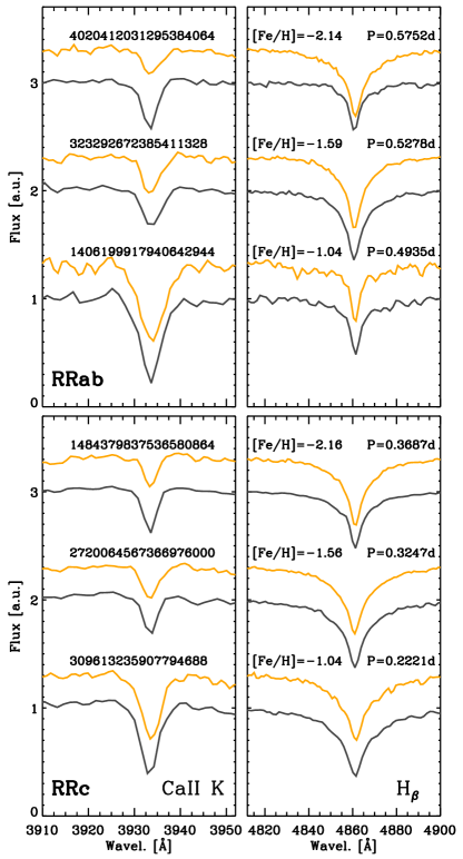
Figure 1: Top: selected low-resolution spectra for three fundamental RRLs with different iron abundances (see labeled values) from the LAMOST (orange) and the SEGUE (grey) datasets. The $Gaia$ EDR3 IDs are also labelled. The left panels display the region across the Ca II K line, while the right ones the region across the H$\beta$ line. Bottom: Same as the top, but for three RRc variables.

Subsequent investigations brought forward that the RRL population ratio, i.e. the ratio between the number of RRc (N_c) variables and the total number of RRLs (N_tot = N_ab + N_c) is, together with mean period, the most popular pulsation diagnostic to dictate the difference between OoI and OoII GCs (Stobie, 1971; Castellani & Quarta, 1987). Indeed, the population ratio for OoII GCs is N_c/N${}_{tot}\sim 0.44$, while for OoI GCs is N_c/N${}_{tot}\sim 0.29$ (Braga et al., 2016). The values of both mean periods and population ratios typical of OoI and OoII GCs depend on the criteria adopted to select cluster variables (Fiorentino et al., 2015), but the quoted estimates are only marginally affected.

The literature concerning the Oosterhoff dichotomy is vast and includes theoretical (Lee et al., 1994; Bono et al., 1995; Cassisi et al., 2004), photometric (Lee & Carney, 1999) and spectroscopic (van den Bergh, 1993) investigations. However, a comprehensive empirical scenario concerning the Oosterhoff dichotomy in field and cluster RRLs was built over half century by Sandage (2010, and references therein). This is the reason why the same problem is known in the literature as the ”Oosterhoff-Arp-Sandage” period-shift effect (Catelan & Smith, 2015, and references therein).

During the last few years the large photometric survey of nearby dwarf galaxies breathed new life into this classical problem. RRLs in Local Group galaxies and in their GCs have mean fundamental periods that fill the so-called Oosterhoff gap, indeed they attain intermediate values ($0.58<P_{ab}<0.62$ days) between OoI and OoII GCs (Petroni & Bono, 2003; Catelan, 2009). This circumstantial evidence indicates that the environment affects the Oosterhoff dichotomy (Fiorentino et al., 2015). Moreover and even more importantly, detailed and comprehensive investigations of three metal-rich clusters (NGC 6388, Pritzl et al. 2002; NGC 6441, Pritzl et al. 2003; NGC 6569, Baker et al. 2007) and of the most massive Galactic GC ($\omega$ Cen, Braga et al. 2016) further strengthened the possible occurrence of additional Oosterhoff groups.

A new spin concerning this classical problem was recently provided by Fabrizio et al. (2019). They provided new metallicity estimates using low resolution spectra collected by SEGUE (Lee et al., 2008) for more than 3,000 field RRLs. This means an increase by almost one order of magnitude with similar data available in the literature. They found that the Oosterhoff dichotomy was mainly caused by the fact that metal-intermediate GCs lack of sizeable samples of RRLs. Indeed, field RRLs display a steady variation in the period distribution and in the Bailey diagram when moving from the metal-poor to the metal-rich regime. However, this investigation was hampered by two limitations: i) the analysis was only based on fundamental variables; ii) they did not investigate the dependence of the population ratio on the iron content.

In the following we address these key issues by using new homogeneous metallicity estimates (see Sect. 2) based on high-resolution spectra and on a new calibration of the $\Delta$S method (Crestani et al., 2021b). This catalog was supplemented with similar metallicity estimates available in the literature (see Sect. 3). As a whole we ended up with a spectroscopic catalog including 9,015 RRLs (6,150 RRab, 2,865 RRc) with at least one metallicity estimate. In Section 4 we discuss the metallicity distribution function of the spectroscopic catalog and investigate the difference between RRc and RRab variables. Section 5 deals with the distribution of the spectroscopic catalog into 2D and 3D realisations of the Bailey diagram. In this section are also discussed the physical mechanisms affecting the Bailey diagram, and in particular, the role played by the Blazhko phenomenon. Section 6 is focussed on the dependence of the pulsation period and visual amplitude on metallicity. The relation between the population ratio and the metallicity for field RRLs is analysed in Section 7, together with a detailed comparison of cluster RRLs and their horizontal branch morphology. Section 8 includes the summary of the current findings and a few brief remarks concerning the future developments of this project.

2 Metallicity measurement

Table 1: RR Lyrae spectroscopic datasets. The columns 3, 4, and 5 list the total number of RRLs, the number of calibrating RRLs and the number of RRLs included in the spectroscopic catalog. The columns 6 and 7 give the zero-points and the slopes of the linear relations adopted to transform literature iron abundances into our metallicity scale. The last column lists the standard deviation of the fit.

Source	Priority	Ntot.	Ncal.	Nsel.	$a\pm\epsilon_{a}$	$b\pm\epsilon_{b}$	$\sigma_{\rm fit}$
HR our	1	190	…	190	…	…	…
HR lita	2	56	…	56	…	…	…
$\Delta$S	3	7928	…	7751	…	…	…
Zinn et al. (2020)	4	462	243	219	$-0.01\pm 0.05$	$1.03\pm 0.03$	0.23
Liu et al. (2020)	5	4805	4093	708	$-0.41\pm 0.10$	$0.66\pm 0.07$	0.23
Dambis et al. (2013)	6	399	242	10	$-0.01\pm 0.05$	$1.03\pm 0.03$	0.25
Duffau et al. (2014)	7	59	25	29	$0.13\pm 0.23$	$0.90\pm 0.13$	0.20
Sesar et al. (2013)	8	50	24	23	$0.14\pm 0.33$	$0.93\pm 0.16$	0.12
RAVE	9	21	…	5	…	…	…
SEGUE-SSPP	10	2781	2756	24	$-0.56\pm 0.02$	$0.62\pm 0.01$	0.24

The metallicity estimates of RRLs were derived by using the most updated version of the $\Delta$S method. The $\Delta$S method was originally introduced by Preston (1959), and it is based on the comparison of the pseudo-equivalent width (EW) of the Ca II K and hydrogen H$\beta$, H$\gamma$, H$\delta$ lines, and it was used exclusively for the fundamental RRL variables by following the prescriptions developed by Layden (1994). The use of this diagnostic requires transformation onto a standard EW system by calibrating these measured calcium and hydrogens EWs with values of a set of spectroscopic ”standards” with the same spectrograph and instrument configuration used to collect the scientific data. Such an approach has been recently upgraded by Crestani et al. (2021b) providing a new calibration of the $\Delta$S method, based on a large sample of high-resolution spectra for more than 140 RRLs. The advantages of this new calibration are i) the extension of the $\Delta$S also to RRc variables, ii) the independence from the transformations between different EW systems and iii) the opportunity to use only one, two or all three Balmer lines.

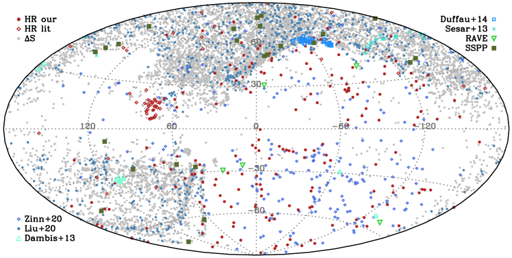
Figure 2: Distribution in Galactic coordinates of the entire spectroscopic sample (9,015 variables). RRLs coming from different spectroscopic datasets are marked with different symbols and/or colours (see labels and Table 1).

In this investigation we used the same spectroscopic sample presented in Crestani et al. (2021b). It is mainly based on 5,885 low-resolution ($R\sim 2000$) spectra collected by the Sloan Extension for Galactic Exploration and Understanding Survey of the Sloan Digital Sky Survey (SEGUE-SDSS, Yanny et al. 2009; Alam et al. 2015), covering 3,004 RRab and 1,562 RRc stars. Moreover, we took advantage of the huge spectroscopic dataset collected by the Large Sky Area Multi-Object Fiber Spectroscopic Telescope DR6 (LAMOST, Cui et al. 2012; Zhao et al. 2012) for which data with a resolution of $R\sim 2000$ are available. A sample of 5,067 spectra were downloaded from the on-line query interface by using a search radius of 2.0 arcsec around each target listed in the RRLs photometric catalogue (see Sect.2 in Crestani et al. 2021b), and we ended up with 2,469 RRab and 1,182 RRc variables with LAMOST spectra (490 in common with SEGUE). Figure 1 shows representative spectra for the LAMOST (orange) and the SEGUE (grey) low-resolution (LR) datasets, for three RRab (top panels) and three RRc (bottom panels), in the region of Ca II K and H$\beta$ lines, with different iron abundance. The profiles of H$\gamma$ and H$\delta$ are very similar to that of H$\beta$ and therefore they are not shown. The similarity between LAMOST and SEGUE datasets allows us to use the same approach and wavelength limits described in Crestani et al. (2021b) to measure the EWs involved in the $\Delta$S method by using an updated IDL version of the EWIMH program (Fabrizio et al., 2019; Layden, 1994). Additionally, we similarly applied this method to 178 stars with low signal-to-noise spectra collected at higher resolution (see below) and degraded to a spectral resolution of $R\simeq 2000$ and sampling $\Delta\log(\lambda)=0.0001$, in order to mimic the native resolution of the SEGUE data. Finally, we applied the relation described in Eqn. 1 of Crestani et al. (2021b) to obtain an estimate of [Fe/H]_ΔS for 7,928 RRL variables. The reader interested in more a detailed discussion concerning the comparison between the metallicity scale for field RRLs, based on both high- and low-resolution spectra, is refereed to Sections 4 and 6 in Crestani et al. (2021b).

Moreover, we also extended the high-resolution (HR, $R\simeq 35,000$) sample — including data collected with the echelle spectrographs at du Pont (Las Campanas Observatory) and at STELLA (Izana Observatory)⁷, UVES and X-shooter at VLT (Cerro Paranal Observatory), HARPS at the 3.6m telescope and FEROS at the 2.2m telescope (La Silla Observatory)⁸, HARPS-N at the Telescopio Nazionale Galileo (Roque de Los Muchachos Observatory)⁷, the HRS at SALT (South African Astronomical Observatory)⁷, and the HDS at Subaru (National Astronomical Observatory of Japan) — for 154 RRab and 36 RRc, ending up with 190 RRLs in the HR sample. The metallicity estimation of these spectra was performed by following the classical approach as described in Crestani et al. (2021b).

3 The RRL spectroscopic catalog

As described in Sect. 2, we have estimated the [Fe/H] of 190 RRLs by means of HR spectroscopic analysis and of 7,928 RRLs by adopting the $\Delta$S method on LR spectra. In the last 25 years, several papers providing [Fe/H] for RRLs were published. Therefore, we have supplemented our own [Fe/H] estimates with those from the literature, to build up an extended catalog of spectroscopic metallicities for RRLs.

To provide a clear picture of the data available in the literature and of the priority ranking that we are going to adopt, we have separated the [Fe/H] estimates found in the literature into those coming from either HR or LR spectroscopy. More specifically, we have collected [Fe/H] estimates based on HR data of 56 RRLs from ten different papers (see the references listed in Tab. 1) and on LR data of 1,018 RRLs from both RRL-specific papers and from large spectroscopic surveys like RAVE (Steinmetz et al., 2006) and SEGUE (from the Stellar Parameter Pipeline - SSPP, Lee et al. 2008).

We ended up with metallicities for 9,015 RRLs. This overall value is smaller than the sum of the quoted sources for two different reasons. i) We performed a double and in some cases a triple visual check of the spectra for faint targets ($\hbox{\it G\/}\leq 19.5$ mag). We found that a few hundred of them have had spectra with signal-to-noise ratios that were borderline for a solid metallicity estimate. They were removed. ii) There are a few hundreds of RRLs with [Fe/H] estimates from more than one source. For this reason, we have ranked the priorities of the different sources as indicated in Table 1.

The quoted priority rank is based on the following criteria, sorted by decreasing relevance: i) the highest priority is given to HR spectroscopic measurements; subsequently to ii) our own estimates based on $\Delta$S; iii) lowest priority to the large datasets. These criteria were finally weighted by other factors (instrumentation, method adopted, uncertainties, single vs multiple measurements) to provide the final ranking.

Table 1 provides the number of RRLs (N_tot.) with [Fe/H] estimates from each source and the final number (N_sel.) adopted in our spectroscopic catalog by following the quoted priority ranking. The sky distribution of the final spectroscopic sample is plotted in Fig. 2 where metallicity estimates coming from different sources are plotted with different symbols and/or colours.

In order to obtain a homogeneous spectroscopic catalog, we calibrated the different literature [Fe/H] estimate based on LR datasets onto the same metallicity scale used for the HR and $\Delta$S samples. Indeed, the ”HR our” (containing our own HR estimates), ”HR lit” (containing the literature HR estimates) and $\Delta$S estimates are already in the same metallicity scale. Therefore we joined them into a single group (HR+$\Delta$S) of 7,997 RRLs and we selected the RRLs in common between (HR+$\Delta$S) and the individual LR samples (N_cal.). To convert the LR metallicities to our scale, we have fitted $\hbox{[Fe/H]}_{HR+\Delta\rm S}$ as function of the $\hbox{[Fe/H]}_{LR}$, for each sample with priority from 4 to 10 (see column 2 in Table 1). The coefficients of the $\hbox{[Fe/H]}_{HR+\Delta\rm S}=a+b\cdot\hbox{[Fe/H]}_{LR}$ fits and their total uncertainties are listed in Table 1. Finally, we have adopted the quoted fits to convert the metallicities from the LR samples into our scale. Note that we could not perform this step for the RAVE metallicities because we found only one match between the RAVE and the HR+$\Delta$S RRLs, therefore the RAVE metallicities were not converted. We also note that, the fits for the Zinn et al. (2020), Dambis et al. (2013), Duffau et al. (2014) and Sesar et al. (2013) samples are close to the bisector, meaning that their metallicities are — taking account of the uncertainties — already in a scale very similar to our own. Additionally, we found that the metallicity scales of Liu et al. (2020) and SEGUE-SSPP are different to ours. The difference between our own scale and that of Liu et al. (2020) was already found by Crestani et al. (2021b) and is due to the different scale of their calibrators.

Note that a similar version of the current spectroscopic catalog, but only focussed on the radial velocity curve templates based on different spectroscopic diagnostics (metallic lines, Balmer lines), is discussed in the fifth paper of this series (Braga et al. 2021, ApJ submitted).

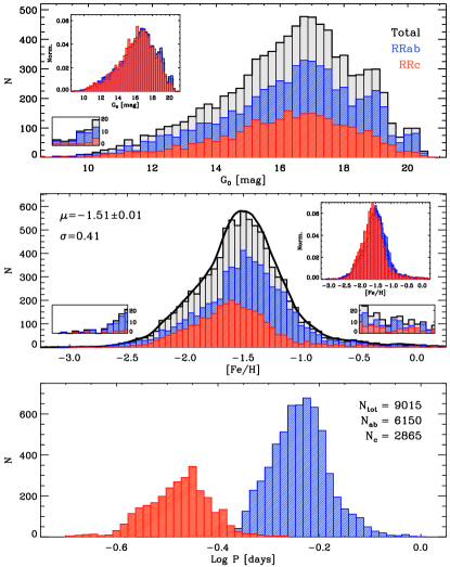
Figure 3: Top: un-reddened G magnitude distributions of the total RRL sample (grey), RRab (blue) and RRc (red) samples with spectroscopic measurements. The small inset displays a zoom-in of the histogram in the bright magnitude end. The large inset shows the same magnitude distributions, but area normalised. Middle: Metallicity distribution of the entire spectroscopic sample (grey) together with the metallicity distribution for RRab (blue) and RRc (red) variables. The solid line shows the smoothed metallicity distribution. The small insets display zoom-in of the histogram in the metal-poor and metal-rich tails. The large inset shows the same metallicity distributions, but area normalised. Bottom: Period distribution of the entire spectroscopic sample for RRab (blue) and RRc (red) variables.

4 The metallicity distribution

Data plotted in the top panel of Fig. 3 display the apparent un-reddened magnitude of the entire spectroscopic sample. The individual reddening values were extracted from the Schlegel et al. (1998) dust maps and the updated reddening coefficients from Schlafly & Finkbeiner (2011), while the extinction in the $G$ band was calculated with the Casagrande & VandenBerg (2018) relation. The key advantage of the current sample when compared with similar datasets available in the literature is that RRLs cover the entire Halo, since their Galactocentric distances range from a few kpc to the outskirts of the Galactic Halo (R_G$\geq$140 kpc). The individual distances were estimated by using predicted optical, near-infrared and mid-infrared Period-Luminosity-Metallicity relations (Marconi et al., 2015, 2018) and they will be discussed in a forthcoming paper. The un-reddened apparent magnitude distributions of both RRab (blue) and RRc (red) variables are quite similar, thus suggesting similar completeness limits.

The metallicity distribution of RRab variables is systematically more metal-rich ($\langle\hbox{[Fe/H]}\rangle_{ab}=-1.48\pm 0.01$, $\sigma=0.41$ dex) than that of the RRc variables ($\langle\hbox{[Fe/H]}\rangle_{c}=-1.58\pm 0.01$, $\sigma=0.40$ dex, see middle panel of Fig. 3). This finding supports previous estimates by Liu et al. (2020) and by Crestani et al. (2021b), which were based on smaller datasets. In this context, it is worth mentioning that the RRc display a smooth low-metallicity tail, while the RRab display a well defined jump for $\hbox{[Fe/H]}\simeq-1.70$ followed by another small increase at $\hbox{[Fe/H]}\simeq-1.60$. In fact, a metallicity peak for RRc more metal-poor than RRab variables is expected from evidence on the distribution of horizontal branch (HB) stars across the RRL instability strip. The current empirical and theoretical evidence indicates that metallicity is the main parameter driving the HB morphology. An increase in the metal content causes the HB morphology to become systematically redder (Torelli et al., 2019). Stellar evolution theory (Bono et al., 2019) and observations (Coppola et al., 2015; Braga et al., 2018) show that RRc populate the hottest and bluest portion of the instability strip. The topology of the instability strip and the dependence of the HB morphology on the metal content provide a qualitative explanation of the reason why RRc variables can be more easily produced in the metal-poor than in the metal-rich regime.

The bottom panel of Fig. 3 shows the period distribution of the spectroscopic sample. Note that the current sample is covering the full period range of RRLs. RRab have periods ranging from $\sim$0.4 days to almost one day, while the RRc range from $\sim$0.2 days to $\sim$0.5 days, and the global fraction of RRc variables is roughly 1/3 of the entire sample. This finding supports theoretical predictions suggesting that the temperature region in which RRc variables attain a stable pulsation cycle is roughly 1/3 of the entire width in temperature of the instability strip (Bono & Stellingwerf, 1994). Note that in this plain explanation we are assuming that the central He burning lifetime of HB stars is almost constant across the instability strip. In passing, we note that the inclusion of RRc variables is crucial to investigate the topology of the instability strip and to address several open problems concerning field and cluster RRLs. However, their inclusion brings forward the thorny problem of short period eclipsing binaries mimicking the luminosity variation typical of RRc variables (Botan et al., 2021). To overcome the contamination of eclipsing binaries we devised a new method based on the optical (Gaia, Clementini et al., 2019) and mid-infrared (MIR from NEOWISE, Mainzer et al., 2011) amplitude ratios. The eclipsing binaries, in the amplitude ratio vs pulsation period plane, cluster within the uncertainties around an amplitude ratio of 1, meaning that the MIR amplitude is similar to the the optical one. Regular RRL variables show in the same plane amplitude ratios ranging from $\approx$0.2 (RRc) to $\approx$0.4 (RRab). However, the MIR amplitudes are only available for $\sim$1% of the RRc variables in the spectroscopic sample. To overcome this limitation we also used the Fourier parameters of the optical light curves together with a visual inspection of their light curves. This novel approach will be discussed in detail in a forthcoming paper (Mullen et al. 2021, in preparation).

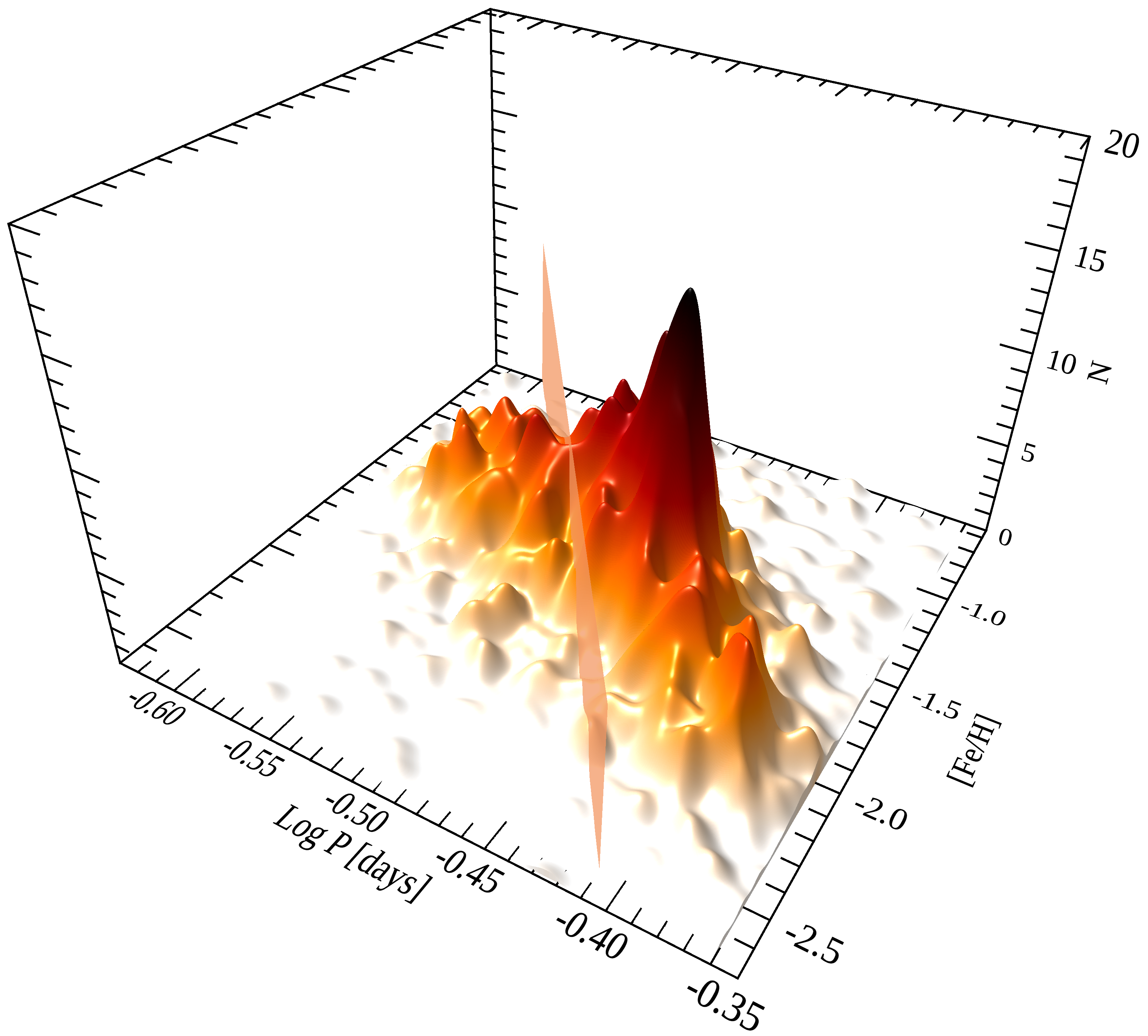
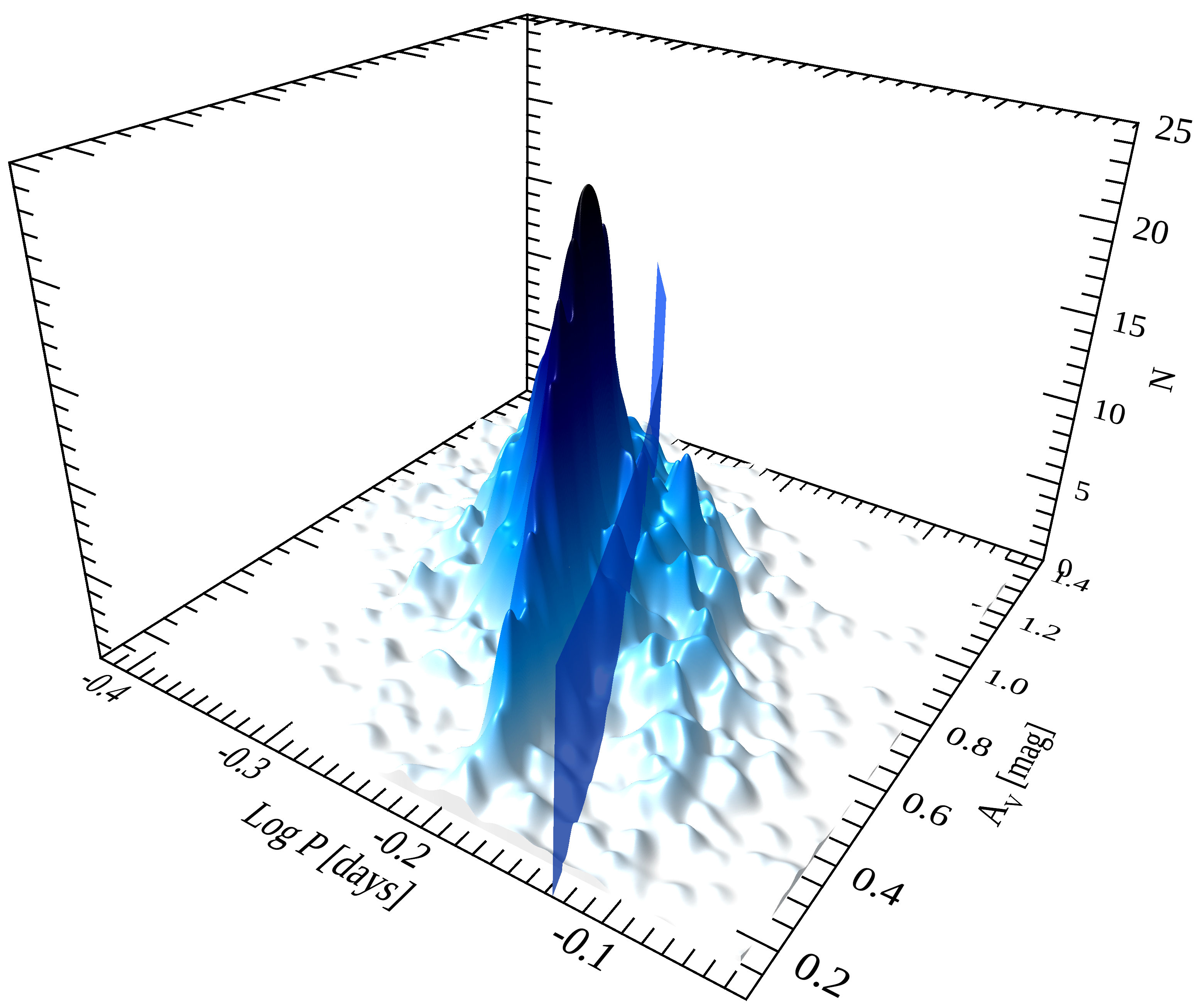
Figure 4: Left: 3D period-metallicity distribution for RRc variables. The distribution was smoothed by using a Gaussian kernel with unitary weight and $\sigma$ equal to the mean error on the metallicity. The light red plane splits the short- from the long-period variables. Right: same as the left, but for RRab variables in the 3D Bailey (logarithmic period vs visual amplitude) distribution. The blue sky plane splits short from long-period RRab variables.

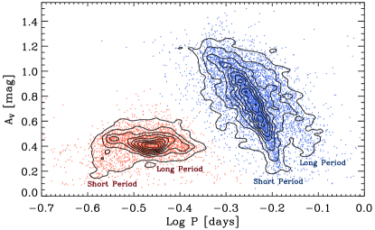
Figure 5: Bailey diagram of the spectroscopic sample: visual amplitude vs logarithmic period for both RRc (red) and RRab (blue) variables. The contours display iso-density levels ranging from 5 to 95% with steps of $\sim$10%.

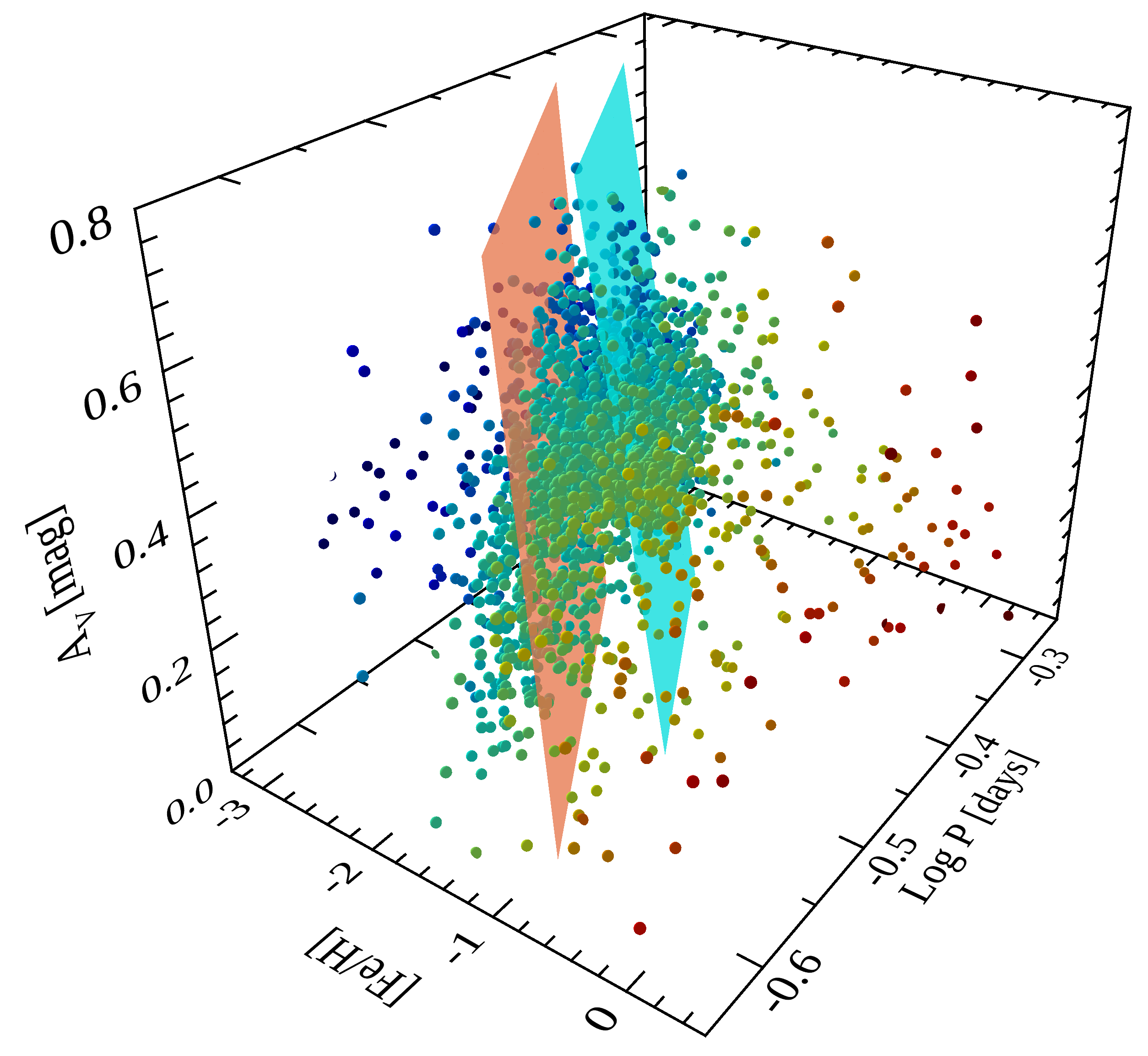
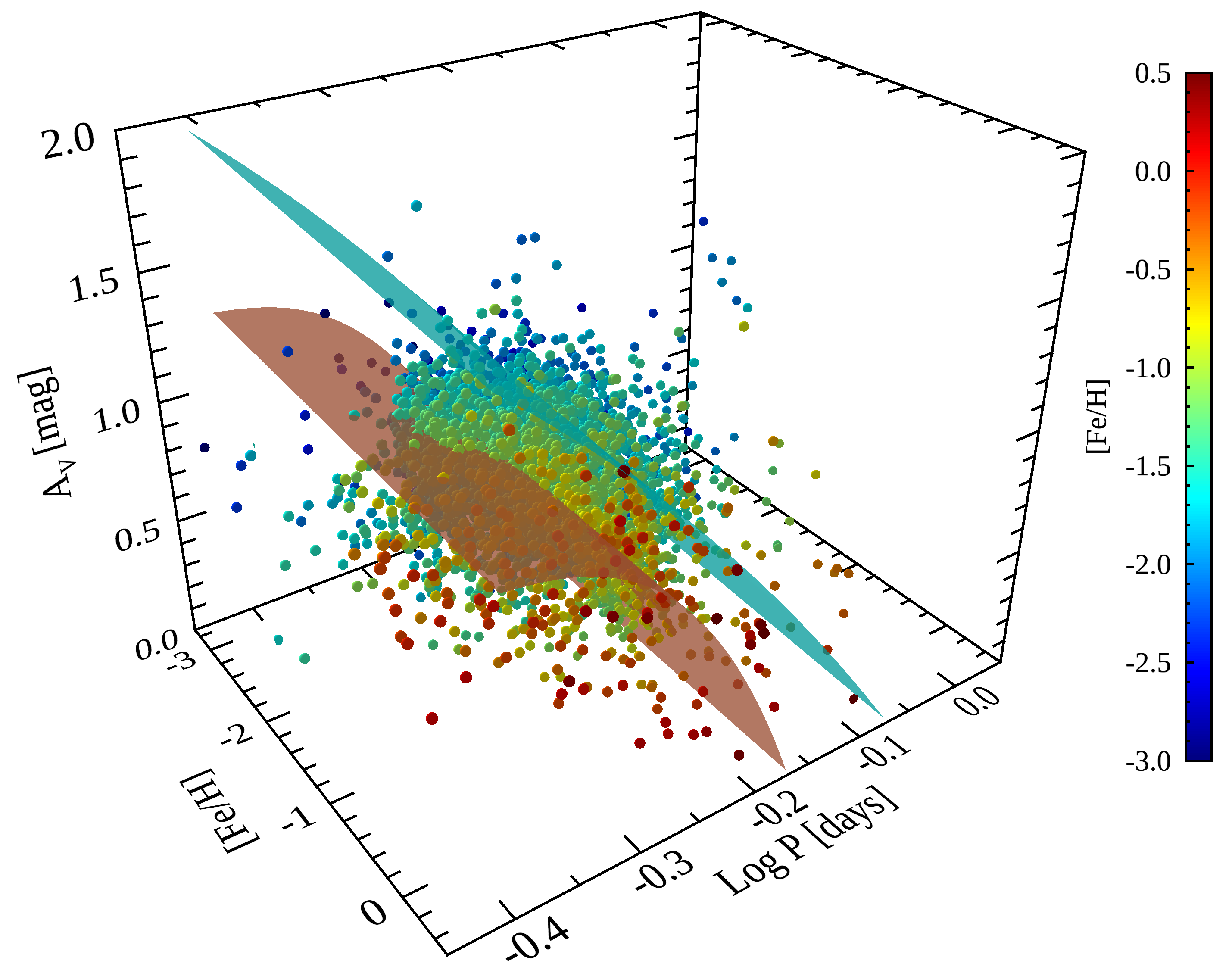
Figure 6: Left: 3D Bailey diagram (visual amplitude, logarithmic period, metallicity) for RRc variables. The metallicity is colour-coded as shown by the colour bar on the right. The coral and cyan planes display the analytical fits tracing more metal-rich (short-period) and more metal-poor (long-period) sub-groups of RRL variables (see text for more details). Right: Same as the left, but for RRab variables.

5 The Bailey diagram

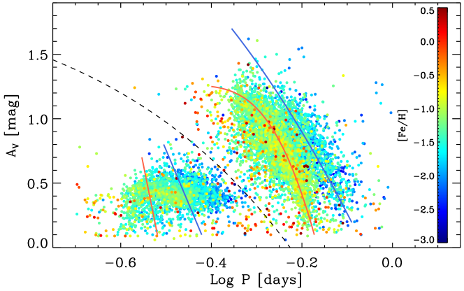
Figure 7: Bailey diagram of the spectroscopic sample. The metallicity is colour-coded as in Fig. 6 and the colour bar is plotted on the right. The dashed line marks the relation used to separate RRc (shorter periods) and RRab (longer periods) variables Clementini et al. (2019). The solid lines display the analytical relations tracing more metal-rich (short-period, red solid lines) and more metal-poor (long-period, blue solid lines) overdensities for both RRab and RRc variables (see text for more details).

Table 2: Parameters of the plane fits $A_{V}=a+b\cdot\hbox{[Fe/H]}+c\cdot\log P+d\cdot(\log P)^{2}+e\cdot(\log P)^{4}$

	$a\pm\epsilon_{a}$	$b\pm\epsilon_{b}$	$c\pm\epsilon_{c}$	$d\pm\epsilon_{d}$	$e\pm\epsilon_{e}$	$\sigma_{\rm fit}$
RRab - Short Period	$-3.53\pm 0.13$	$-0.019\pm 0.003$	$-29.62\pm 1.32$	$-52.37\pm 3.63$	$+49.88\pm 7.69$	0.19
RRab - Long Period	$-0.51\pm 0.06$	$-0.032\pm 0.007$	$-7.69\pm 0.68$	$-4.52\pm 1.83$	…	0.18
RRc - Short Period	$-12.86\pm 3.50$	$-2.43\pm 0.60$	$-17.48\pm 4.69$	…	…	0.77
RRc -Long Period	$-5.43\pm 0.46$	$-1.26\pm 0.09$	$-8.35\pm 0.25$	…	…	0.58

To further improve the analysis of the fine structure of the Bailey diagram, the left panel of Fig. 4 shows in a 3D plot the distribution of RRc variables in the logarithmic period vs metallicity plane. The 3D distribution was smoothed by using a Gaussian kernel with unitary weight and $\sigma$ equal to the mean error on the metallicity estimates. The light red plane separate short-period (SP) from long-period (LP) RRc variables. The same approach was adopted to separate short- from long-period RRab variables and the right panel of Fig. 4 shows the 3D plot of the Bailey diagram (logarithmic period vs visual amplitude). The 3D distribution was smoothed by using the same approach adopted for RRc variables, but the $\sigma$ is equal to the mean error on the luminosity amplitudes. The light blue plane separate SP from LP RRab variables. This plane is very similar to the dotted–dashed line plotted in the bottom panel of Fig. 13 in Fabrizio et al. (2019) showing the Oosterhoff intermediate loci and defined as the ”valley” between the two main overdensities. Note that the visual amplitudes ($A_{V}$) adopted in this investigation come from two different sources: a) G-band time series photometry collected by Gaia. The light curves were folded by using the periods provided within Gaia DR2 and fitted with Fourier series. The G-band amplitude was estimated as the difference G(min)–G(max) of the analytical fit. The G-band amplitudes were then transformed into V-band amplitudes by using Eqn.2 from Clementini et al. (2019). b) For RRLs with poor Gaia phase coverage, $A_{V}$ estimates were collected from the literature. As before, $A_{V}$ is the difference between the brightest and faintest point of the analytical fit. It is worth mentioning that, in the analysis of the Bailey diagram, we did not include RRLs for which the mean magnitude was estimated by an optical light curve template (i.e. those from Pan-STARRS and DECam, Sesar et al., 2017; Stringer et al., 2019). In fact, despite G-band amplitudes are available for these stars, the amplitudes come from the template fitting of the data, hence they are not homogeneous with $A_{V}$ estimates from the previous sources a) and b).

The separation between SP and LP variables can be further investigated with the iso-contour plots for both RRc (red dots) and RRab (blue dots) variables in the canonical Bailey diagram of Fig. 5. Data plotted in this figure show that the distribution of RRLs is, as expected, far from being homogeneous. The iso-contours associated with RRab variables show that the bulk of RRab variables are mainly distributed along the SP sequence, while the LP sequence only includes a minor fraction of RRab variables ($\sim$80% vs $\sim$20%). The RRc variables display an almost flat amplitude distribution for periods ranging from $\log P=-0.57$ to $\log P=-0.35$. However, the RRc variables display an opposite trend when compared with RRab variables, indeed the fraction of SP ($\log P\leq-0.51$) RRc variables is significantly smaller than the fraction of LP ones. The current data, indeed, are suggesting relative fractions of $\sim$30% and $\sim$70%, respectively (see Sect. 7 for more quantitative details).

To summarise the observed correlation among pulsation period, visual amplitude and iron content, Fig. 6 shows the 3D distribution of the entire spectroscopic sample. Note that the iron content is colour-coded (see the bar on the right) and moves from dark blue (very metal-poor) to dark red (very metal-rich). We performed an analytical fit connecting the three key parameters (period, visual amplitude, metallicity) independent of distance and reddening. The coefficients of the fit, their errors and the standard deviations of the different relations are listed in Table 2. Note that the cyan and coral planes trace overdensities associated with more metal-rich (SP) and more metal-poor (LP) sub-groups of RRL variables. In passing, we also note that the standard deviation in metal content is, at a fixed pulsation period, too large to apply these relations to individual RRLs. Indeed, the analytical relations shall be applied to periods and amplitudes of sizeable RRL samples.

Fig. 7 shows the classical Bailey diagram for the entire spectroscopic sample, but the symbols are colour-coded following the same metallicity scale adopted in Fig. 6. To properly identify in the canonical Bailey diagram the short- and the long-period sequences among the RRab variables, the analytical fits discussed above were cut at fixed iron content ($\hbox{[Fe/H]}=-1.5$). The ensuing two-dimensional relations for the short- and the long-period sequences are the following:

$${\rm SP:\>}A_{V}[{\rm mag}] = -3.50(\pm 0.13)+$$

$$\left[\sigma=0.19\>{\rm mag}\right] -29.62(\pm 1.32)\cdot\log P+$$ (1)

$$-52.37(\pm 3.63)\cdot(\log P)^{2}+$$

$$+49.88(\pm 7.69)\cdot(\log P)^{4}$$

$${\rm LP:\>}A_{V}[{\rm mag}] = -0.46(\pm 0.06)+$$

$$\left[\sigma=0.18\>{\rm mag}\right] -7.69(\pm 0.68)\cdot\log P+$$ (2)

$$-4.52(\pm 1.83)\cdot(\log P)^{2}$$

and they are plotted as a red and a blue solid line in the RRab region of Fig. 7.

We have already mentioned that RRc variables display a smooth transition when moving from the short- to the long-period range. A plausible separation can only be attained by using the 3D distribution. However, we decided to follow the same approach adopted for RRab variables and we cut the analytical fits at $\hbox{[Fe/H]}=-1.60$. The two dimensional analytical relations we obtained are the following:

$${\rm SP:\>}A_{V}[{\rm mag}] = -8.97(\pm 3.55)+$$

$$\left[\sigma=0.90\>{\rm mag}\right] -17.48(\pm 4.69)\cdot\log P$$ (3)

$${\rm LP:\>}A_{V}[{\rm mag}] = -3.42(\pm 0.32)+$$

$$\left[\sigma=0.40\>{\rm mag}\right] -8.35(\pm 0.25)\cdot\log P$$ (4)

and they are plotted as a red and a blue solid line in the RRc region of Fig. 7.

Data plotted in this figure display quite clearly that an increase in the metal content causes a systematic shift of both RRab and RRc towards shorter pulsation periods. The adopted colour coding shows that the more metal-rich RRLs (from yellow to red) are mainly located in the short-period tail. We also note that the metallicity dependence is stronger among RRc than RRab variables. Indeed, RRc with periods shorter than 0.25 days are systematically more metal-rich than the bulk of RRc variables. A similar effect is also present among the RRab, defining the so-called High Amplitude Short Period (HASP) variables ($P<0.48$ days, $A_{V}>0.75$ mag, Fiorentino et al. 2015). Indeed, the relative fraction of RRab variables located in the HASP region more metal-rich than $\hbox{[Fe/H]}=-1.5$ is 75%, while their mean metallicity is $\langle\hbox{[Fe/H]}\rangle_{\rm HASP}=-1.25\pm 0.02$ ($\sigma=0.42$ dex). The current findings soundly support the estimates by Fabrizio et al. (2019) using iron abundances based on low-resolution spectra for $\sim$2,900 RRab variables and, more recently, by Crestani et al. (2021b) using iron abundances based on high-resolution spectra for 143 RRLs (111 RRab, 32 RRc). In passing, we also note that a similar trend for the pulsation period as function of the metallicity was already found in the Galactic Bulge by using data from the MACHO survey for a thousand of RRab stars (Kunder & Chaboyer, 2009) and more recently by using more than 8,100 RRab variables (Prudil et al., 2019).

6 The dependence of periods and luminosity amplitudes on metallicity

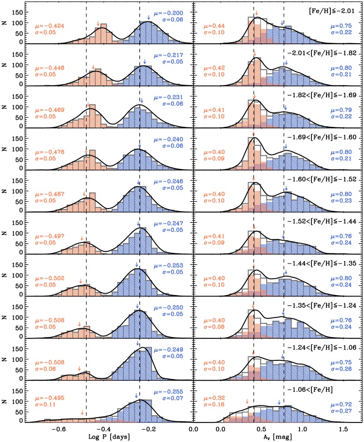
Figure 8: Period (left panels) and visual amplitude (right panels) distributions of the spectroscopic sample. The sample was split in ten metallicity bins (see labelled values) including a similar number of objects. The solid lines display the smoothed distributions. The arrows mark the mean period and the mean amplitude of the individual bins for RRab (blue) and RRc (red) variables. The dashed lines show the mean $\log P$ ($-0.240$ and $-0.477$) and mean $A_{V}$ (0.40 and 0.77 mag) of the total sample.

To further investigate the dependence of both periods and amplitudes on the metallicity we divided the entire spectroscopic sample into ten different metallicity bins. The range in metallicity of the different bins was adjusted in such a way that each bin includes one tenth of the total sample. The left and the right panels of Fig. 8 display the period and the visual amplitude distributions in the ten metallicity bins (see labeled values).

Data plotted in the left panels display very clearly that the mean of the period distribution for both RRab (in blue) and RRc (in red) when moving from the metal-poor (top panels) to the metal-rich (bottom panels) regime decreases from $\log P\simeq-0.20$ to $\log P\simeq-0.26$ for RRab and from $\log P\simeq-0.42$ to $\log P\simeq-0.51$ for RRc variables. The dashed vertical lines show the mean periods of the entire sample ($\langle\log P\rangle_{ab}=-0.240$, $\langle\log P\rangle_{c}=-0.477$). The variation of the mean period among the ten metallicity bins is of the order of 23% ($\Delta\log P=0.055$) for RRab and of the order of 14% ($\Delta\log P=0.083$) for RRc variables.

The difference between the period distribution of RRab and RRc variables becomes even more evident if we take into account the variation of the standard deviations. Data plotted in the left panels show that the period distribution becomes less and less peaked when moving from the metal-poor to the metal-rich regime. This trend is more relevant for RRc variables, because the standard deviation in the most metal-rich bin is a factor of two larger than the typical standard deviation of the metal-poor metallicity bins, despite all bins sharing the same number of objects, and although the last bin covers a large range in metallicity.

The visual amplitudes display a similar behaviour (right panels): an increase in metal content causes a steady decrease in the mean visual amplitude. The effect is more relevant for RRc than for RRab variables. Indeed, the A_V for RRc variables decreases from $\sim$0.44 mag to 0.32 mag ($\sim$25%). The RRab variables show a different trend: the amplitude increases from $\sim$0.75 mag to $\sim$0.80 mag, when moving from the metal-poor to the metal-intermediate regime, while it decreases from $\sim$0.80 mag to $\sim$0.72 mag when moving from the metal-intermediate to the metal-rich regime.

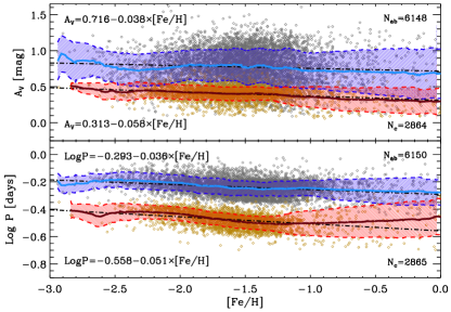
Figure 9: Top: Visual amplitude as function of iron abundance for RRab (grey dots) and RRc (dark yellow dots). The blue and the red solid lines display the running averages for RRab and RRc variables and the shaded areas show the corresponding standard deviation. The dot-dashed lines display the linear regressions and their coefficients are labelled. Bottom: Same as the top, but with the $\log P$ on the y-axis.

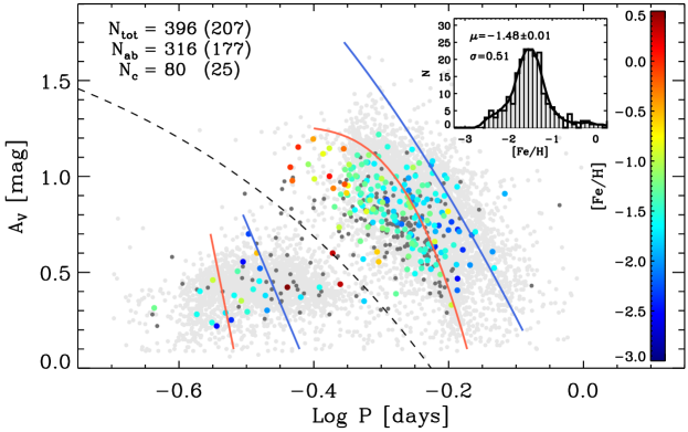
Figure 10: Bailey diagram of candidate Blazhko RRLs. The light grey symbols display the entire spectroscopic sample plotted in Fig. 7. The Blazhko RRLs for which the iron abundance is available are marked with coloured symbols, while those for which it is not available are marked with dark grey symbols. The numbers of RRab and RRc candidate Blazhko RRLs are labelled, the numbers in parentheses display the numbers of candidate Blazhko RRLs with iron abundances. The small inset shows the metallicity distribution of candidate Blazhko RRLs.

To investigate on a more quantitative basis the metallicity dependence of both periods and visual amplitudes we performed a linear fit over the entire metallicity range (see Fig. 9). To overcome spurious fluctuations in the metal-poor and in the metal-rich regime we performed a running average. The entire sample of RRab variables (grey diamonds) was ranked as a function of the metal content, and we estimated the mean with a running box including 500 variables. The solid blue line plotted in the top panel of Fig. 9 shows the running average and the two dashed lines display the 1$\sigma$ standard deviation. The same approach was adopted for RRc variables (yellow diamonds), the red solid and dashed lines plotted in the same panel show their running average and their standard deviations.

To validate the spectroscopic sample adopted to estimate the dependence of the luminosity amplitude on the metal content we performed several tests. To quantify the impact that RRL with amplitude modulation have on the global distribution we neglected candidate Blazhko RRLs (see Sect. 6.1). Furthermore, we also tested the dependence on the faint tail and we neglected variables fainter than the G=17 mag (i.e. the peak in the apparent magnitude distribution of Fig. 3). We found that the coefficients of the analytical relations for both the visual amplitudes and the pulsation periods are, within the errors, identical.

To constrain on a more quantitative basis the difference between the trend of RRab and RRc variables we performed a linear fit of the entire sample and we found:

$${\rm RRab:\>}A_{V}[{\rm mag}] = 0.716(\pm 0.011)+$$

$$\left[\sigma=0.24\right]\;\; -0.038(\pm 0.007)\cdot\hbox{[Fe/H]}$$ (5)

and

$${\rm RRc:\>}A_{V}[{\rm mag}] = 0.312(\pm 0.008)+$$

$$\left[\sigma=0.10\right] -0.058(\pm 0.004)\cdot\hbox{[Fe/H]}$$ (6)

Note that the number of RRLs adopted in the analytical fits of the visual amplitude as a function of the metal content is smaller than the number of RRLs adopted in analytical fits of the pulsation periods because in the former sample we neglected the RRLs whose mean magnitude was estimated by using an optical light curve template, i.e. variables for which the visual amplitude is not available yet. The former relation soundly supports the results obtained by Fabrizio et al. (2019) for a smaller sample of RRLs (2,903 vs 6,150 RRab). Moreover, the current amplitude-metallicity relation for RRab variables further supports the modest dependence of the visual amplitude on the metallicity. Indeed, a variation of 3 dex in metal content would only cause a difference in visual amplitude of $\approx$0.12 mag. The metallicity dependence is stronger for RRc variables: an increase of 3 dex in metal content causes an increase in visual amplitude that is almost a factor of two larger ($\approx$0.2 mag). The stronger sensitivity of RRc visual amplitudes to metallicity and the decrease by a factor of two in the standard deviation (0.10 vs 0.24 mag) are due to the fact that the region of the instability strip in which they are pulsationally stable is at least a factor of two narrower than the region covered by RRab variables. This means that the impact of the metallicity on pulsation and evolutionary properties for RRc variables is less affected by changes in their intrinsic properties. Evolutionary effects due to off-Zero Age HB (ZAHB) evolution at fixed stellar mass and chemical composition and for a typical red-ward evolution (see Fig. 4 in Bono et al., 2020), causes a decrease in surface gravity, and in turn, an increase in the pulsation period and a decrease in the visual amplitude. This means that the off-ZAHB evolution can have a complex pattern across the Bailey diagram (Bono et al., 2020).

The bottom panel of Fig. 9 shows the logarithmic period of the entire spectroscopic sample as a function of the metal content. We estimated the same running averages (blue and red solid lines) over the two subsamples and performed the linear fits (dot-dashed lines) obtaining the following results:

$${\rm RRab:\>}\log P[{\rm days}] = -0.293(\pm 0.003)+$$

$$\left[\sigma=0.06\right] -0.036(\pm 0.002)\cdot\hbox{[Fe/H]}$$ (7)

and

$${\rm RRc:\>}\log P[{\rm days}] = -0.558(\pm 0.004)+$$

$$\left[\sigma=0.06\right] -0.051(\pm 0.003)\cdot\hbox{[Fe/H]}$$ (8)

As expected, the dependence of the pulsation period for both RRab and RRc variables on the metallicity are similar to the dependence on the visual amplitude, but their standard deviations are systematically smaller. Moreover, preliminary evidence indicates that the dispersion of the $\log P$-metallicity relation for RRc variables in the metal-rich regime is larger than for RRab. In this context it is worth mentioning that the two sub-samples are well populated for $\hbox{[Fe/H]}\geq-0.7$ (218 RRab; 90 RRc). We still lack a quantitative explanation for this effect. The global properties of RRab and RRc variables will be addressed in the next section.

6.1 Physical mechanisms affecting the Bailey diagram

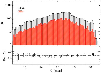
Figure 11: Top: Apparent G-band distribution of RRLs in the spectroscopic sample. The red histogram shows the distribution of RRc variables, while the grey one the global (RRab+RRc) sample. Bottom: Relative difference between RRc distribution and the global sample.

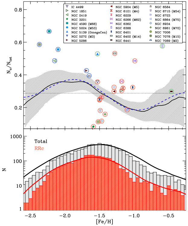
Figure 12: Top: The population ratio as a function of the iron abundance (solid black line), i.e. the ratio between the number of RRc and the total number ($N_{c}/(N_{c}+N_{ab})$) of RRL variables. The grey hatched area shows the 1$\sigma$ uncertainty. Coloured symbols display the population ratio of Galactic GCs (see labelled names) hosting at least 33 RRLs. The GCs hosting RRLs with pulsation properties typical of OoI stellar systems are marked with an open red circle, while those with pulsation properties typical of OoII systems are marked with an open blue circle. Three peculiars clusters (NGC 6388, NGC 6441, $\omega$ Cen) are marked with an open green circle. The blue dashed line shows the analytical fit of Eqn.9. Bottom: Iron distribution for RRc (red) and total (RRab+RRc, grey) RRL variables. The solid lines show the same distribution, but smoothed using a Gaussian kernel with unitary weight and $\sigma$ equal to the individual errors on the iron abundances.

Together with the evolutionary effects already mentioned in Sect. 6 the distribution of the variables in the Bailey diagram is also affected by two independent physical mechanisms: a) the Blazhko effect and b) non-linear phenomena. The Blazhko phenomenon mainly affects the RRab variables ($\sim$40%, Prudil & Skarka, 2017) and the modulation in amplitude is more relevant for shorter than for longer period RRLs. Indeed, the modulations change from $\sim$0.7 mag, close to the fundamental blue edge, to $\sim$0.05 mag, close to the fundamental red edge (see Fig. 10 in Skarka et al. 2020, and also Jurcsik et al. 2011; Benkő et al. 2014; Braga et al. 2016). The RRc variables are also affected by the Blazhko phenomenon, but the fraction is significantly smaller ($\sim$6%, Netzel et al., 2018) and the amplitude modulation is, at most, of the order of $\sim$0.2 mag.

To further investigate the impact that the Blazhko effect has on the trends visible in the Bailey diagram, Fig. 10 shows the candidate Blazhko Halo RRLs. They are plotted using their mean visual amplitude and we are showing the entire sample of candidate Blazhko RRLs, i.e. RRLs with amplitude modulations ranging from a few hundredths to a few tenths of magnitude. The candidate Blazhko RRLs for which the iron abundance is available are marked with coloured symbols (see the bar on the right side), while those lacking of a metallicity estimate are plotted with dark grey symbols. The metallicity distribution of candidate Blazhko RRLs (see the inset in Fig. 10) is quite similar to the global RRL metallicity distribution. Although, the sample of candidate Blazhko RRLs with iron abundances is at least forty times smaller of the entire spectroscopic sample, both the peak and the standard deviation agree within the errors. We cannot exclude possible biases in the metallicity distribution, because the candidate Blazhko RRLs, as noted by the anonymous referee, are mainly restricted to the solar neighbourhood. However, the tails of the RRab metallicity distribution appear to be properly sampled, while for RRc variables the metallicity distribution is still too limited. Data plotted in the Bailey diagram display that the Blazhko phenomenon for RRab variables appears to be mainly associated either with metal-intermediate or with metal-rich RRLs. Indeed, in agreement with the global trend (see Sect. 5) the bulk of the candidate Blazhko RRab variables are mainly distributed across the SP sequence (92% vs 8% across the LP sequence), while the candidate Blazhko RRc are mostly located across the LP sequence (78% vs 22% across the SP sequence). The relative fractions for RRc variables need to be cautiously treated, since they are roughly two dozen. In passing, we also note that the current findings support recent results by Skarka et al. (2020) based on a large sample (more than 3,300) of Galactic Bulge and cluster Blazhko RRLs.

Non-linear phenomena like the formation and propagation of strong shocks are mainly affecting RRab variables and, in particular, the RRab located close to the blue edge of the instability strip. These variables are characterised by very large amplitudes and light curves showing a saw-tooth shape. The occurrence of non-linear phenomena is strongly supported by the presence of a dip along the rising branch of the light curve and by solid spectroscopic evidence (Gillet, 2013; Sneden et al., 2017; Gillet et al., 2019). The RRc variables are also affected by shocks, but the current evidence indicate that the shocks marginally affect their properties (Duan et al., 2020; Benkő et al., 2021).

The current circumstantial evidence indicates that the Blazhko effect and non-linear phenomena can only partially account for the typical dispersion of the luminosity amplitudes, at fixed pulsation period, and in particular, the difference between the RRab and the RRc when these parameters are considered.

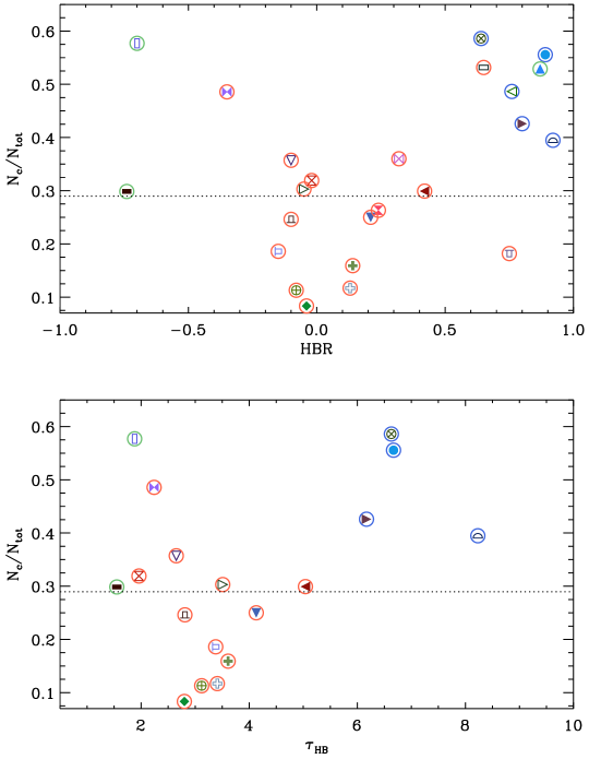
Figure 13: Top: The population ratio N_c/N_tot as function of the HBR parameter. The symbols are the same as Fig. 12. Bottom: Same as the top, but as function of $\tau_{\rm HB}$ parameter.

7 The dependence of the population ratio on metallicity

Table 3: Galactic Globular Clusters hosting more than 33 RR Lyrae stars. From left to right the different columns give the cluster name(s), the iron abundance, the number of RRab and RRc variables, the population ratio, the horizontal branch morphology indices and the Oosterhoff type (see text for more details).

Cluster	[Fe/H]a	Nabb	Ncb	Nc/Ntot	$HBR$c	$\tau_{HB}$c	Ooster.Type
IC 4499	$-1.53$	63	35	0.36	$-0.10$	2.65	OoI
NGC 1851	$-1.18$	23	10	0.30	$-0.05$	3.51	OoI
NGC 2419	$-2.15$	38	36	0.49	0.76	…	OoII
NGC 3201	$-1.59$	77	7	0.08	$-0.04$	2.80	OoI
NGC 4590 (M68)	$-2.23$	14	28	0.67	0.58	4.43	OoII
NGC 5024 (M53)	$-2.10$	28	35	0.56	0.89	6.67	OoII
NGC 5139 ($\omega$ Cen)	$-1.53$e	90	101	0.53	0.87	…	Pecul.d
NGC 5272 (M3)	$-1.50$	177	59	0.25	0.21	4.13	OoI
NGC 5286	$-1.69$	31	23	0.43	0.80	6.17	OoII
NGC 5904 (M5)	$-1.29$	89	38	0.30	0.42	5.04	OoI
NGC 6121 (M4)	$-1.16$	32	15	0.32	$-0.02$	1.96	OoI
NGC 6229	$-1.47$	42	15	0.26	0.24	…	OoI
NGC 6266 (M62)	$-1.18$	144	81	0.36	0.32	…	OoI
NGC 6362	$-0.99$	18	17	0.49	$-0.35$	2.24	OoI
NGC 6388	$-0.59$	11	15	0.58	$-0.70$	1.88	Pecul.d
NGC 6401	$-1.02$	23	11	0.32	…	…	OoI
NGC 6402 (M14)	$-1.28$	52	59	0.53	0.65	…	OoI
NGC 6441	$-0.46$	47	20	0.30	$-0.74$	1.55	Pecul.d
NGC 6584	$-1.50$	49	16	0.25	$-0.10$	2.81	OoI
NGC 6715 (M54)	$-1.49$	153	34	0.18	0.75	…	OoI
NGC 6723	$-1.10$	35	8	0.19	$-0.15$	3.38	OoI
NGC 6864 (M75)	$-1.29$	25	12	0.32	…	…	OoI
NGC 6934	$-1.47$	68	9	0.12	0.13	3.41	OoI
NGC 6981 (M72)	$-1.42$	37	7	0.16	0.14	3.61	OoI
NGC 7006	$-1.52$	55	7	0.11	$-0.08$	3.12	OoI
NGC 7078 (M15)	$-2.37$	65	92	0.59	0.64	6.63	OoII
NGC 7089 (M2)	$-1.65$	23	15	0.39	0.92	8.23	OoII

The population ratio (N_c/N_tot) is a solid parameter to trace the topology of the instability strip, i.e. the region of the instability strip in which fundamental and first overtone RRLs attain a stable limit cycle. The dependence of the population ratio on metallicity provides not only quantitative clues on the topology of the instability strip, but also on the dependence of the HB morphology on the metal content.

The accuracy of the population ratio relies on the completeness limits of both RRab and RRc variables. The RRc variables are more affected by an observational bias than RRab variables. The RRLs obey to well defined Period-Luminosity relations for wavelengths longer than the R-band and the RRc variables are typically fainter than RRab variables. Moreover, the RRc luminosity amplitudes are on average smaller than the RRab variables. To investigate on a more quantitative basis this issue, Fig. 11 shows the comparison between the apparent magnitude distribution of RRc variables (red histogram) and the total number of RRLs. The two histograms display the same trend when moving from the bright to the faint limit of the distribution. Thus suggesting that the completeness of both RRab and RRc variables is similar over the entire magnitude range.

The top panel of Fig. 12 shows the population ratio (solid black line) as a function of the iron content for Galactic RRLs, by using the running average algorithm described in Sect. 6, together with its standard deviation (grey hatched area). Data plotted in this figure bring forward several new features worth being discussed in detail.

Continuous variation – The variation of the population ratio over the entire metallicity range is continuous and does not show evidence of a dichotomic distribution. Indeed, the population ratio steadily increases in the metal-poor regime and it approaches a well defined plateau with N_c/N_tot$\sim$0.36 for $-2.15\leq\hbox{[Fe/H]}\leq-1.70$. The trend is opposite in the metal-intermediate regime, with the population ratio steadily decreasing and it attains its absolute minimum (N_c/N_tot$\sim$0.18) for $-0.9\leq\hbox{[Fe/H]}\leq-0.8$. Note that the standard deviation in this metallicity regime is systematically smaller than in the metal-poor/metal-rich regime because the mean of the metallicity distributions of both RRab and RRc (see the bottom panel of the same figure) is located at $\hbox{[Fe/H]}\simeq-1.48$ and $\simeq-1.58$, respectively. The population ratio shows, once again, a steady increase in the metal-rich regime and it attains values close to its mean value (N_c/N_tot$\sim$0.29) at solar iron abundance. Note that the increase in the population ratio for iron abundances larger than $-0.8$ dex cannot be explained by plain evolutionary arguments. Indeed, an increase in the metal content causes a systematic drift of the HB morphology towards redder colours. This means that the RRL instability strip is going to be mainly populated in its redder region where only RRab variables attain a stable limit cycle. The consequence is that the population ratio in the metal-rich regime should display either a steady decrease or approaching an almost constant value. To further constrain the behaviour of the population ratio as function of metallicity, we also provide a continuous analytical fit (blue dashed line) by combining a linear plus a sinusoidal function:

$$\frac{N_{c}}{N_{tot}} = 0.212(\pm 0.004)-0.047(\pm 0.002)\cdot\hbox{[Fe/H]}+$$ (9)

$$+0.073(\pm 0.003)\cdot\sin\left(2.19(\pm 0.08)\right.+$$

$$\left.+3.78(\pm 0.04)\cdot\hbox{[Fe/H]}\right)\;\;\;\;\left[\sigma=0.0002\right]$$

The variation of the population ratio described above could be affected by an observation bias: the number of RRL variables increases when approaching the Galactic plane. However, these regions are also severely affected by high extinction. This means that the current RRL sample is far from being complete at low Galactic latitudes (Preston et al., 1991). Moreover, the fraction of metal-rich RRLs increases in approaching the Galactic plane (Layden, 1994). This means that the continuous variation shown in Fig. 12 is not affected by this bias, but the accuracy concerning the metal-rich sub-sample will improve once more complete RRL sample will become available.

Global trend – According to the Oosterhoff dichotomy we would expect to have a population ratio of $\approx$0.44 for more metal-poor stellar systems (OoII) and a value close to $\approx$0.3 for more metal-rich stellar systems (OoI). However, data plotted in the top panel of Fig. 12 are far from being representative of the quoted dichotomic trend. The population ratio attains, within the errors, relative maxima (N_c/N_tot$\sim$0.36), both in the metal-poor and in the metal-rich regime.

Comparison with globular clusters – To further constrain possible similarities between field and cluster RRLs we compared the current population ratio with similar estimates for Galactic globulars hosting more than 33 RRLs (Clement et al., 2001). We arbitrarily selected this number of cluster RRLs to limit statistical fluctuations in the population ratio. The population ratios of the globulars are plotted in Fig. 12 with different symbols (see labelled names and values listed in Tab. 3) and their trend is far from being homogeneous. Cluster RRLs in the metal-poor regime ($\hbox{[Fe/H]}\leq-1.6$) either agree within the errors or display population ratios typical of OoII stellar systems (marked with blue open circles) that are systematically larger than field RRLs. The comparison between cluster and field RRLs is more complex in the metal-intermediate regime ($-1.5\leq\hbox{[Fe/H]}\leq-1.0$), because the population ratio for typical OoI stellar systems (marked with red open circles) ranges from less than 0.1 for NGC 3201 to more than 0.5 for M14. In this metallicity regime the field RRLs display a steady decrease from $\sim$0.3 to $\sim$0.2 and the smallest dispersion. The comparison in the metal-rich ($\hbox{[Fe/H]}\geq-1$) regime is hampered by the limited number of Galactic globulars hosting sizeable RRL samples. One out of the three globulars present in this metallicity regime (NGC 6441) agrees quite well with field RRLs, but NGC 6388 (with a similar iron abundance), and in particular, NGC 6362 ($\sim$0.3 dex more metal-poor) attain population ratios that are systematically larger than field ones. Note that the two metal-rich globulars have HB morphologies dominated by an extended blue tail and by a sizeable sample of red HB stars. In this context it is worth mentioning $\omega$ Cen, since it hosts a sizeable sample of RRLs (191) and they display a well defined spread in iron abundance ($-2.58\leq\hbox{[Fe/H]}\leq-0.85$, Magurno et al. 2019) with a population ratio of 0.53. $\omega$ Cen is the most massive globular and its HB morphology is dominated by an extended blue tail.

To investigate on a more quantitative basis the possible correlation between the population ratio and the HB morphology, the top panel of Fig. 13 shows the population ratio as a function of the HB morphology index [$HBR$=$(B-R)/(B+V+R)$] introduced more than 35 years ago by Lee (1989, see also ). In the $HBR$ index the parameter $B$, $R$ and $V$ take accounts for the number of HB stars that are either hotter ($B$) or cooler ($R$) than the RRL instability strip, while $V$ is the number of RRLs. As expected OoI/OoII stellar systems attain population ratios that are on average smaller/larger than the mean Halo value (dotted line). The current data do not display a global trend when moving from globulars with HB morphologies dominated by red HB stars (on average more metal-rich and with negative $HBR$ values) and globulars with HB morphologies dominated by blue HB stars (on average more metal-poor and with positive $HBR$ values). There is evidence that the bulk of OoI clusters distribute along a redder/bluer sequence departing from $HBR\simeq-0.15$ and $HBR\simeq 0.15$, respectively. The two sequences show modest variations in the $HBR$ parameter, but the population ratio changes by more than a factor of four. Indeed, two globulars of the redder sequence, namely NGC 3201 and IC 4499 have similar $HBR$ values ($HBR$=$-0.04$ vs $-0.10$), but the former one only host a few RRc variables (7 out of 84, N_c/N_tot=0.08) variables while the latter includes 35 RRc variables out of 98 RRLs (N_c/N_tot=0.36). The same outcome applies to the bluer sequence: the two globulars NGC 6934 and M62 have $HBR$ values of 0.13 and 0.32, while the population ratio changes from 0.12 to 0.36. A similar sequence is also present among OoII clusters, indeed, the two globulars M2 and M53 have similar $HBR$ values ($HBR$=0.92 vs 0.89), but the former one only host a few RRc variables (15 out of 38, N_c/N_tot=0.39) while the latter includes more RRc than RRab variables (35 out of 63, N_c/N_tot=0.56).

The morphology index $HBR$ presents several pros and cons when compared with the morphology index $\tau_{\rm HB}$ recently introduced by Torelli et al. (2019). This new $\tau_{\rm HB}$ parameter is defined as the ratio between the areas subtended by the cumulative number distribution in magnitude and in colour of all the stars distributed along the HB. The bottom panel of Fig. 13 shows the population ratio as a function of $\tau_{\rm HB}$ for a sub-sample of the globulars adopted in the top panel. The current data indicate a mild preliminary evidence of a steady increase in the population ratio when moving from globulars with intermediate HB morphologies (the horizontal portion of the HB, i.e., blue HB, red HB and the instability strip are well populated) to globulars with HB morphologies dominated by blue stars. The spread among the OoI clusters is still quite large, and indeed, the two peculiar clusters with HB morphologies dominated by red HB stars (smaller $\tau_{\rm HB}$ values), but with extended blue tails, attain larger population ratios. This sub-group also includes four metal-intermediate clusters (M4, IC 4499, NGC 6362, NGC 6584) with intermediate HB morphologies. The degeneracy of these two sub-groups in the population ratio vs $\tau_{\rm HB}$ plane needs to be investigated in more detail.

It bears mentioning that the number of OoII globulars for which the $\tau_{\rm HB}$ is available is still too limited to investigate in detail their properties. Finally, we note that the two globulars with HB morphologies dominated by blue HB stars include a metal-poor (M15, $\hbox{[Fe/H]}=-2.37$) and a metal- intermediate (M2, $\hbox{[Fe/H]}=-1.65$) cluster with population ratios that agree quite well with field RRLs with similar iron abundances.

The current circumstantial evidence further support that globulars played a subdominant role in the build-up of the stellar Halo, also in agreement with the results of recent observational surveys (Hanke et al., 2020) and Galactic simulations (Reina-Campos et al., 2020).

8 Summary and final remarks

We performed a new and homogeneous spectroscopic analysis of field Halo RRLs, with iron abundances estimated using both low- and high-resolution spectra collected at random phases. The iron abundances based on high-resolution spectra include 190 RRLs Crestani et al. (2021a), while those based on low-resolution spectra include more than 7,700 RRLs. The latter sample is based on the new calibration of the $\Delta$S method recently provided by Crestani et al. (2021b). These abundances were complemented with iron abundances based on both low- and high-resolution spectra available in the literature and brought to our metallicity scale. To provide a homogeneous metallicity scale, special attention was paid in the inclusion of the different datasets. The transformations into our metallicity scale were estimated by using the objects in common between our catalog and the datasets available in the literature.

We ended up with the largest spectroscopic catalog ever collected for both fundamental and first overtone RRLs. The current sample includes 9,015 RRLs (6,150 RRab, 2,865 RRc) with at least one metallicity estimate. Moreover and even more importantly, the current spectroscopic catalog covers the extent of the Galactic stellar Halo, with Galactocentric distances ranging from $\approx$5 to more than 140 kpc. This spectroscopic catalog was used to address several pending issues concerning the pulsation properties of field RRLs and their use as tracers of old stellar populations:

Metallicity distribution function – The cumulative metallicity distribution function (MDF) shows a mean value at $\langle\hbox{[Fe/H]}\rangle=-1.51\pm 0.01$ with a standard deviation $\sigma$=0.41 dex. The current estimates agree with similar estimates available in the literature and bring forward a clear asymmetry. Indeed, the MDF shows a long tail in the metal-poor regime approaching $\hbox{[Fe/H]}\sim-3$ and a sharp metal-rich tail approaching solar iron abundance. The large sample of spectroscopic measurements allows us to investigate in detail the MDF of both RRab and RRc variables. We found that RRab variables are systematically more metal-rich ($\langle\hbox{[Fe/H]}\rangle_{ab}=-1.48\pm 0.01$, $\sigma=0.41$ dex) than RRc variables ($\langle\hbox{[Fe/H]}\rangle_{c}=-1.58\pm 0.01$, $\sigma=0.40$ dex). This finding fully supports preliminary estimates by Liu et al. (2020) and by Crestani et al. (2021b) using smaller datasets.

A preliminary qualitative explanation of the difference in the MDF of RRab and RRc variables can be provided by using plain evolutionary and pulsation arguments. The topology of the instability strip and the dependence of the HB morphology on the metal content indicate that RRc variables can be more easily produced in the metal-poor than in the metal-rich regime. However, it is worth mentioning that the MDF of RRc variables displays a metal-rich tail that is more significant than the metal-rich tail of RRab variables.

Bailey Diagram – The distribution of field RRLs in the Bailey diagram (visual amplitude vs logarithmic period) shows several interesting features. An increase in the metal content causes a smooth and systematic shift towards shorter periods for both RRab and RRc variables. The analysis of the iso-contour across the Bailey diagram indicates that the relative fraction of RRab variables located along the short-period sequence (more metal-rich) and the long-period sequence (more metal-poor) is 80% and 20%. Interestingly enough, the relative fractions for RRc variables have an opposite trend, namely 30% (short-period) and 70% (long-period), respectively.

Dependence of pulsation periods and visual amplitudes on metallicity – The large sample of spectroscopic measurements allowed us to investigate on a quantitative basis, for the first time, the dependence of pulsation periods and visual amplitudes on metallicity. We found that the pulsation period of both RRab and RRc variables shows a steady decrease when moving from the metal-poor to the metal-rich regime. We derived new analytical relations and we found that an increase of 1 dex in iron content causes on average a decrease of $\approx$0.04 dex in the logarithmic period. The trend concerning the visual amplitudes is similar. The analytical relations indicate that the visual amplitude of RRab variables is almost a factor of two less sensitive to the metal content than for RRc variables, indeed, the coefficient of the metallicity term decreases from –0.038 to –0.058. The difference might be associated to a stronger impact of non-linear phenomena on RRab than on RRc luminosity amplitudes. In spite of this difference visual amplitudes and periods for both RRab and RRc variables do show smooth distributions over the entire metallicity range. This evidence fully supports the preliminary results concerning the nature of the Oosterhoff dichotomy obtained by Fabrizio et al. (2019) using a smaller dataset of only RRab variables. Indeed, they showed that the Oosterhoff dichotomy is an a natural consequence of the lack of metal-intermediate Galactic globular clusters hosting a sizeable sample of RRL stars.

Impact of the metallicity on the Blazhko effect – The large and homogeneous spectroscopic dataset allowed us to investigate the impact that the iron abundance has on the occurrence of the Blazhko phenomenon. We found that candidate Blazhko RRLs pulsating in the fundamental mode (177 RRab) appear to be distributed across the OoI sequence, i.e. they seem to be either metal-intermediate or metal-rich objects. The candidate Blazhko RRLs pulsating in the first overtone (25 RRc) seem to show an opposite trend, because they seem to be mainly located across the OoII sequence. The fraction of candidate Blazhko RRab variables more metal-rich than $\hbox{[Fe/H]}=-1.5$ is 28% while for RRc variables is 9%. However, the number of RRc variables with spectroscopic iron abundances is still too limited to reach a firm conclusion concerning their dependence on the metallicity.

Dependence of the population ratio (N_c/N_tot) on metallicity – We investigated the dependence of the population ratio on the metal content and we found that the trend of field RRLs is more complex than expected on the basis of similar estimates for globular clusters available in the literature. We found that the population ratio steadily increases from $\sim$0.25 to $\sim$0.36 when moving from the very metal-poor regime to $\hbox{[Fe/H]}\simeq-1.8$. Moreover, the population ratio shows a decrease by a factor of two (0.36 vs 0.18) and a smaller dispersion, at fixed iron content, in the metal-intermediate regime ($-1.8\leq\hbox{[Fe/H]}\leq-0.9$). Finally, it shows once again a steady increase when moving into the metal-rich regime, approaching a value of $\sim$0.3 at solar iron abundance. The current findings appear to be at odds with pulsation and evolutionary predictions, because the number of RRc variables should steadily decreases when moving from the metal-poor/metal-intermediate regime into the metal-rich regime.

Concerning cluster RRLs, we also investigated the occurrence of a possible correlation between the population ratio and the HB morphology. We adopted two different HB morphology indices ($HBR$, $\tau_{\rm HB}$) and selected clusters hosting roughly three dozen of RRLs. We found that globulars distribute along several sequences in which the $HBR$ index shows either minimal or modest variations, but the population ratio changes by more than a factor of two/four. These sequences appear both in OoI and in OoII clusters. Furthermore, the $\tau_{\rm HB}$ morphology index shows a mild correlation with the population ratio when moving from globulars characterised by intermediate HB morphologies typical of OoI clusters to globulars dominated by extended blue HB tails, typical of OoII clusters. Once again, OoI clusters with similar $\tau_{\rm HB}$ values display variations in the population ratio by more than a factor of two.

The analysis of field and cluster RRLs provides two interesting findings: a) the population ratio is a promising diagnostic to further investigate the fine structure of the HB even for clusters with similar HB morphology indices; b) the different trends between field and cluster RRLs in the population ratio vs metallicity plane indicate that globular clusters played a minor role, if any, in building up the Halo. The early formation and evolution of the Halo and the role played by nearby stellar systems will be addressed by using pulsation properties, kinematics and metallicity distributions of field RRLs in a forthcoming paper.

A famous motto suggests that novel approaches to attack, and possibly explain, longstanding astrophysical problems open up more problems than they are able to solve. The results of this investigation concerning the Oosterhoff dichotomy and the population ratio moves along this path.

References

- Alam et al. (2015) Alam, S., Albareti, F. D., Allende Prieto, C., et al. 2015, ApJS, 219, 12, doi: 10.1088/0067-0049/219/1/12
- Andrievsky et al. (2018) Andrievsky, S., Wallerstein, G., Korotin, S., et al. 2018, PASP, 130, 024201, doi: 10.1088/1538-3873/aa9783
- Arp (1955) Arp, H. C. 1955, AJ, 60, 317, doi: 10.1086/107232
- Baker et al. (2007) Baker, J. M., Layden, A. C., Welch, D. L., & Webb, T. M. A. 2007, AJ, 133, 139, doi: 10.1086/509638
- Benkő et al. (2014) Benkő, J. M., Plachy, E., Szabó, R., Molnár, L., & Kolláth, Z. 2014, ApJS, 213, 31, doi: 10.1088/0067-0049/213/2/31
- Benkő et al. (2021) Benkő, J. M., Sódor, Á., & Pál, A. 2021, MNRAS, 500, 2554, doi: 10.1093/mnras/staa3452
- Bono et al. (1995) Bono, G., Caputo, F., & Marconi, M. 1995, AJ, 110, 2365, doi: 10.1086/117694
- Bono & Stellingwerf (1994) Bono, G., & Stellingwerf, R. F. 1994, ApJS, 93, 233, doi: 10.1086/192054
- Bono et al. (2016) Bono, G., Pietrinferni, A., Marconi, M., et al. 2016, Commmunications of the Konkoly Observatory Hungary, 105, 149
- Bono et al. (2019) Bono, G., Iannicola, G., Braga, V. F., et al. 2019, ApJ, 870, 115, doi: 10.3847/1538-4357/aaf23f
- Bono et al. (2020) Bono, G., Braga, V. F., Crestani, J., et al. 2020, ApJ, 896, L15, doi: 10.3847/2041-8213/ab9538
- Botan et al. (2021) Botan, E., Saito, R. K., Minniti, D., et al. 2021, MNRAS, 504, 654, doi: 10.1093/mnras/stab888
- Braga et al. (2016) Braga, V. F., Stetson, P. B., Bono, G., et al. 2016, AJ, 152, 170, doi: 10.3847/0004-6256/152/6/170
- Braga et al. (2018) —. 2018, AJ, 155, 137, doi: 10.3847/1538-3881/aaadab
- Cacciari & Renzini (1976) Cacciari, C., & Renzini, A. 1976, A&AS, 25, 303
- Casagrande & VandenBerg (2018) Casagrande, L., & VandenBerg, D. A. 2018, MNRAS, 479, L102, doi: 10.1093/mnrasl/sly104
- Cassisi et al. (2004) Cassisi, S., Castellani, M., Caputo, F., & Castellani, V. 2004, A&A, 426, 641, doi: 10.1051/0004-6361:20041048
- Castellani & Quarta (1987) Castellani, V., & Quarta, M. L. 1987, A&AS, 71, 1
- Catelan (2009) Catelan, M. 2009, Ap&SS, 320, 261, doi: 10.1007/s10509-009-9987-8
- Catelan & Smith (2015) Catelan, M., & Smith, H. A. 2015, Pulsating Stars (Wiley-VCH)
- Chadid et al. (2017) Chadid, M., Sneden, C., & Preston, G. W. 2017, ApJ, 835, 187, doi: 10.3847/1538-4357/835/2/187
- Clement et al. (2001) Clement, C. M., Muzzin, A., Dufton, Q., et al. 2001, AJ, 122, 2587, doi: 10.1086/323719
- Clementini et al. (2019) Clementini, G., Ripepi, V., Molinaro, R., et al. 2019, A&A, 622, A60, doi: 10.1051/0004-6361/201833374
- Coppola et al. (2015) Coppola, G., Marconi, M., Stetson, P. B., et al. 2015, ApJ, 814, 71, doi: 10.1088/0004-637X/814/1/71
- Crestani et al. (2021a) Crestani, J., Braga, V. F., Fabrizio, M., et al. 2021a, ApJ, submitted, AAS30873
- Crestani et al. (2021b) Crestani, J., Fabrizio, M., Braga, V. F., et al. 2021b, ApJ, 908, 20, doi: 10.3847/1538-4357/abd183
- Cui et al. (2012) Cui, X.-Q., Zhao, Y.-H., Chu, Y.-Q., et al. 2012, Research in Astronomy and Astrophysics, 12, 1197, doi: 10.1088/1674-4527/12/9/003
- Dambis et al. (2013) Dambis, A. K., Berdnikov, L. N., Kniazev, A. Y., et al. 2013, MNRAS, 435, 3206, doi: 10.1093/mnras/stt1514
- Duan et al. (2020) Duan, X.-W., Chen, X.-D., Deng, L.-C., et al. 2020, arXiv e-prints, arXiv:2012.13396. https://arxiv.org/abs/2012.13396
- Duffau et al. (2014) Duffau, S., Vivas, A. K., Zinn, R., Méndez, R. A., & Ruiz, M. T. 2014, A&A, 566, A118, doi: 10.1051/0004-6361/201219654
- Fabrizio et al. (2019) Fabrizio, M., Bono, G., Braga, V. F., et al. 2019, ApJ, 882, 169, doi: 10.3847/1538-4357/ab3977
- Fernley & Barnes (1996) Fernley, J., & Barnes, T. G. 1996, A&A, 312, 957
- Fiorentino et al. (2015) Fiorentino, G., Bono, G., Monelli, M., et al. 2015, ApJ, 798, L12, doi: 10.1088/2041-8205/798/1/L12
- For et al. (2011) For, B.-Q., Sneden, C., & Preston, G. W. 2011, ApJS, 197, 29, doi: 10.1088/0067-0049/197/2/29
- Gillet (2013) Gillet, D. 2013, A&A, 554, A46, doi: 10.1051/0004-6361/201220840
- Gillet et al. (2019) Gillet, D., Mauclaire, B., Lemoult, T., et al. 2019, A&A, 623, A109, doi: 10.1051/0004-6361/201833869
- Govea et al. (2014) Govea, J., Gomez, T., Preston, G. W., & Sneden, C. 2014, ApJ, 782, 59, doi: 10.1088/0004-637X/782/2/59
- Hanke et al. (2020) Hanke, M., Koch, A., Prudil, Z., Grebel, E. K., & Bastian, U. 2020, A&A, 637, A98, doi: 10.1051/0004-6361/202037853
- Harris (1996) Harris, W. E. 1996, AJ, 112, 1487, doi: 10.1086/118116
- Jurcsik et al. (2011) Jurcsik, J., Szeidl, B., Clement, C., Hurta, Z., & Lovas, M. 2011, MNRAS, 411, 1763, doi: 10.1111/j.1365-2966.2010.17817.x
- Kunder & Chaboyer (2009) Kunder, A., & Chaboyer, B. 2009, AJ, 138, 1284, doi: 10.1088/0004-6256/138/5/1284
- Lambert et al. (1996) Lambert, D. L., Heath, J. E., Lemke, M., & Drake, J. 1996, ApJS, 103, 183, doi: 10.1086/192274
- Layden (1994) Layden, A. C. 1994, AJ, 108, 1016, doi: 10.1086/117132
- Lee & Carney (1999) Lee, J.-W., & Carney, B. W. 1999, AJ, 118, 1373, doi: 10.1086/301008
- Lee et al. (2008) Lee, Y. S., Beers, T. C., Sivarani, T., et al. 2008, AJ, 136, 2022, doi: 10.1088/0004-6256/136/5/2022
- Lee (1989) Lee, Y.-W. 1989, PhD thesis, Yale University., New Haven, CT.
- Lee et al. (1990) Lee, Y.-W., Demarque, P., & Zinn, R. 1990, ApJ, 350, 155, doi: 10.1086/168370
- Lee et al. (1994) —. 1994, ApJ, 423, 248, doi: 10.1086/173803
- Liu et al. (2020) Liu, G. C., Huang, Y., Zhang, H. W., et al. 2020, ApJS, 247, 68, doi: 10.3847/1538-4365/ab72f8
- Liu et al. (2013) Liu, S., Zhao, G., Chen, Y.-Q., Takeda, Y., & Honda, S. 2013, Research in Astronomy and Astrophysics, 13, 1307, doi: 10.1088/1674-4527/13/11/003
- Magurno et al. (2019) Magurno, D., Sneden, C., Bono, G., et al. 2019, ApJ, 881, 104, doi: 10.3847/1538-4357/ab2e76
- Mainzer et al. (2011) Mainzer, A., Grav, T., Bauer, J., et al. 2011, ApJ, 743, 156, doi: 10.1088/0004-637X/743/2/156
- Marconi et al. (2018) Marconi, M., Bono, G., Pietrinferni, A., et al. 2018, ApJ, 864, L13, doi: 10.3847/2041-8213/aada17
- Marconi et al. (2015) Marconi, M., Coppola, G., Bono, G., et al. 2015, ApJ, 808, 50, doi: 10.1088/0004-637X/808/1/50
- Nemec et al. (2013) Nemec, J. M., Cohen, J. G., Ripepi, V., et al. 2013, ApJ, 773, 181, doi: 10.1088/0004-637X/773/2/181
- Netzel et al. (2018) Netzel, H., Smolec, R., Soszyński, I., & Udalski, A. 2018, MNRAS, 480, 1229, doi: 10.1093/mnras/sty1883
- Oosterhoff (1939) Oosterhoff, P. T. 1939, The Observatory, 62, 104
- Pancino et al. (2015) Pancino, E., Britavskiy, N., Romano, D., et al. 2015, MNRAS, 447, 2404, doi: 10.1093/mnras/stu2616
- Petroni & Bono (2003) Petroni, S., & Bono, G. 2003, Mem. Soc. Astron. Italiana, 74, 915. https://arxiv.org/abs/astro-ph/0302480
- Preston (1959) Preston, G. W. 1959, ApJ, 130, 507, doi: 10.1086/146743
- Preston et al. (1991) Preston, G. W., Shectman, S. A., & Beers, T. C. 1991, ApJ, 375, 121, doi: 10.1086/170175
- Pritzl et al. (2002) Pritzl, B. J., Smith, H. A., Catelan, M., & Sweigart, A. V. 2002, AJ, 124, 949, doi: 10.1086/341381
- Pritzl et al. (2003) Pritzl, B. J., Smith, H. A., Stetson, P. B., et al. 2003, AJ, 126, 1381, doi: 10.1086/377024
- Prudil et al. (2019) Prudil, Z., Dékány, I., Catelan, M., et al. 2019, MNRAS, 484, 4833, doi: 10.1093/mnras/stz311
- Prudil & Skarka (2017) Prudil, Z., & Skarka, M. 2017, MNRAS, 466, 2602, doi: 10.1093/mnras/stw3231
- Reina-Campos et al. (2020) Reina-Campos, M., Hughes, M. E., Kruijssen, J. M. D., et al. 2020, MNRAS, 493, 3422, doi: 10.1093/mnras/staa483
- Sandage (1981) Sandage, A. 1981, ApJ, 248, 161, doi: 10.1086/159140
- Sandage (2010) —. 2010, ApJ, 722, 79, doi: 10.1088/0004-637X/722/1/79
- Sandage & Wallerstein (1960) Sandage, A., & Wallerstein, G. 1960, ApJ, 131, 598, doi: 10.1086/146872
- Schlafly & Finkbeiner (2011) Schlafly, E. F., & Finkbeiner, D. P. 2011, ApJ, 737, 103, doi: 10.1088/0004-637X/737/2/103
- Schlegel et al. (1998) Schlegel, D. J., Finkbeiner, D. P., & Davis, M. 1998, ApJ, 500, 525, doi: 10.1086/305772
- Sesar et al. (2013) Sesar, B., Grillmair, C. J., Cohen, J. G., et al. 2013, ApJ, 776, 26, doi: 10.1088/0004-637X/776/1/26
- Sesar et al. (2017) Sesar, B., Hernitschek, N., Mitrović, S., et al. 2017, AJ, 153, 204, doi: 10.3847/1538-3881/aa661b
- Skarka et al. (2020) Skarka, M., Prudil, Z., & Jurcsik, J. 2020, MNRAS, 494, 1237, doi: 10.1093/mnras/staa673
- Sneden et al. (2017) Sneden, C., Preston, G. W., Chadid, M., & Adamów, M. 2017, ApJ, 848, 68, doi: 10.3847/1538-4357/aa8b10
- Steinmetz et al. (2006) Steinmetz, M., Zwitter, T., Siebert, A., et al. 2006, AJ, 132, 1645, doi: 10.1086/506564
- Stobie (1971) Stobie, R. S. 1971, ApJ, 168, 381, doi: 10.1086/151094
- Stringer et al. (2019) Stringer, K. M., Long, J. P., Macri, L. M., et al. 2019, AJ, 158, 16, doi: 10.3847/1538-3881/ab1f46
- Torelli et al. (2019) Torelli, M., Iannicola, G., Stetson, P. B., et al. 2019, A&A, 629, A53, doi: 10.1051/0004-6361/201935995
- van Agt & Oosterhoff (1959) van Agt, S. L. T. J., & Oosterhoff, P. T. 1959, Annalen van de Sterrewacht te Leiden, 21, 253
- van den Bergh (1993) van den Bergh, S. 1993, AJ, 105, 971, doi: 10.1086/116485
- Yanny et al. (2009) Yanny, B., Rockosi, C., Newberg, H. J., et al. 2009, AJ, 137, 4377, doi: 10.1088/0004-6256/137/5/4377
- Zhao et al. (2012) Zhao, G., Zhao, Y.-H., Chu, Y.-Q., Jing, Y.-P., & Deng, L.-C. 2012, Research in Astronomy and Astrophysics, 12, 723, doi: 10.1088/1674-4527/12/7/002
- Zinn et al. (2020) Zinn, R., Chen, X., Layden, A. C., & Casetti-Dinescu, D. I. 2020, MNRAS, 492, 2161, doi: 10.1093/mnras/stz3580