Learned Token Pruning for Transformers

Abstract.

Efficient deployment of transformer models in practice is challenging due to their inference cost including memory footprint, latency, and power consumption, which scales quadratically with input sequence length. To address this, we present a novel token reduction method dubbed Learned Token Pruning (LTP) which adaptively removes unimportant tokens as an input sequence passes through transformer layers. In particular, LTP prunes tokens with an attention score below a threshold, whose value is learned for each layer during training. Our threshold-based method allows the length of the pruned sequence to vary adaptively based on the input sequence, and avoids algorithmically expensive operations such as top-$k$ token selection. We extensively test the performance of LTP on GLUE and SQuAD tasks and show that our method outperforms the prior state-of-the-art token pruning methods by up to $\sim$2.5% higher accuracy with the same amount of FLOPs. In particular, LTP achieves up to 2.1$\times$ FLOPs reduction with less than 1% accuracy drop, which results in up to 1.9$\times$ and 2.0$\times$ throughput improvement on Intel Haswell CPUs and NVIDIA V100 GPUs. Furthermore, we demonstrate that LTP is more robust than prior methods to variations in input sequence lengths. Our code has been developed in PyTorch and open-sourced.

1. Introduction

Transformer-based deep neural network architectures (Vaswani et al., 2017), such as BERT (Devlin et al., 2018) and RoBERTa (Liu et al., 2019), achieve state-of-the-art results in Natural Language Processing (NLP) tasks such as sentence classification and question answering. However, efficiently deploying these models is increasingly challenging due to their large size, the need for real-time inference, and the limited energy, compute, and memory resources available. The heart of a transformer layer is the multi-head self-attention mechanism, where each token in the input sequence attends to every other token to compute a new representation of the sequence. Because all tokens attend to each others, the computation complexity is quadratic with respect to the input sequence length; thus the ability to apply transformer models to long input sequences becomes limited.

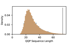
(a) QQP

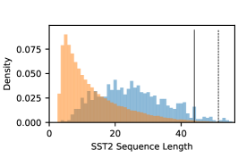
(b) SST-2

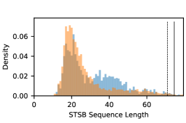
(c) STS-B

Figure 1. Distributions of processed input sequence lengths from datasets for representative tasks in the GLUE benchmark: (a) QQP (b) SST-2; (c) STS-B. The training set is in orange and the validation set is in blue. The dashed and solid vertical lines indicate the 99th percentile value for the training and validation sets, respectively.

Pruning is a popular technique to reduce the size of neural networks and the amount of computation required. Unstructured pruning allows arbitrary patterns of sparsification for parameters and feature maps and can, in theory, produce significant computational savings while preserving accuracy. However, commodity DNN accelerators cannot efficiently exploit unstructured sparsity patterns. Thus, structured pruning methods are typically preferred in practice due to their relative ease of deployment to hardware.

Multi-head self-attention provides several possibilities for structured pruning; for example, head pruning (Michel et al., 2019; Voita et al., 2019) decreases the size of the model by removing unneeded heads in each transformer layer. Another orthogonal approach that we consider in this paper is token pruning, which reduces computation by progressively removing unimportant tokens in the sequence during inference. For NLP tasks such as sentence classification, token pruning is an attractive approach to consider as it exploits the intuitive observation that not all tokens (i.e., words) in an input sentence are necessarily required to make a successful inference.

There are two main classes of token pruning methods. In the first class, methods like PoWER-BERT (Goyal et al., 2020) and Length-Adaptive Transformer (LAT) (Kim and Cho, 2020) search for a single token pruning configuration (i.e., sequence length for each layer) for an entire dataset. In other words, they prune all input sequences to the same length. However, input sequence lengths can vary greatly within tasks and between training and validation sets as in Figure 1, and thus applying a single pruning configuration to all input sequences can potentially under-prune shorter sequences or over-prune longer sequences.

In the other class, the token pruning method adjusts the configuration based on the input sequence. SpAtten (Wang et al., 2020b) uses a pruning configuration proportional to input sentence length; however, it does not adjust the proportion of pruned tokens based on the content of the input sequence. The recently published TR-BERT (Ye et al., 2021) uses reinforcement learning (RL) to find a policy network that dynamically reduces the number of tokens based on the length and content of the input sequence; however, it requires additional costly training for convergence of the RL-based method. Additionally, all of these prior methods rely in part on selecting the $k$ most significant tokens during inference or training. This selection can be computationally expensive without the development of specialized hardware, such as the top-$k$ engine introduced in SpAtten (Wang et al., 2020b).

To this end, we propose a learned threshold-based token pruning method which adapts to the length and content of individual examples and avoids the use of top-$k$ operations. In particular, our contributions are as follows:

• We propose Learned Token Pruning (LTP), a threshold-based token pruning method, which only needs a simple threshold operation to detect unimportant tokens. In addition, LTP fully automates the search for optimal pruning configurations by introducing a differentiable soft binarized mask that allows training the correct thresholds for different layers and tasks. (Section 3.3)

• We apply LTP to RoBERTa and evaluate its performance on GLUE and SQuAD tasks. We show LTP achieves up to 2.10$\times$ FLOPs reduction with less than 1% accuracy degradation, which results in up to 1.93$\times$ and 1.97$\times$ throughput improvement on NVIDIA V100 GPU and Intel Haswell CPU, respectively, as compared to the unpruned FP16 baseline. We also show that LTP outperforms SpAtten and LAT in most cases, achieving additional FLOPs reduction for the same drop in accuracy. (Section 4.2 and 4.5)

• We show that LTP is highly robust against sentence length variations. LTP exhibits consistently better accuracy over different sentence length distributions, achieving up to 16.4% accuracy gap from LAT. (Section 4.3)

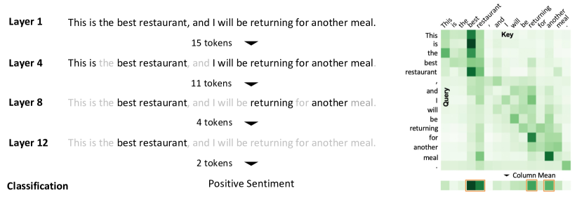
Figure 2. (Left) Schematic of token pruning for a sentiment analysis task. Unimportant tokens are pruned as the input sequence passes through the layers. (Right) An example of attention probability in a single head where a more important token receives more attention from other tokens. Thus each token’s importance score is computed by taking the average attention probability it receives, which is computed by taking the column mean of the attention probability.

2. Related Work

2.1. Efficient Transformers

Multiple different approaches have been proposed to improve speed and diminish memory footprint of transformers. These can be broadly categorized as follows: (i) efficient architecture design (Lan et al., 2019; Child et al., 2019; Kitaev et al., 2020; Wang et al., 2020a; Iandola et al., 2020; Vyas et al., 2020; Tay et al., 2020; Katharopoulos et al., 2020; Zaheer et al., 2020; Roy et al., 2021); (ii) knowledge distillation (Sun et al., 2020; Jiao et al., 2019; Tang et al., 2019; Sanh et al., 2019; Sun et al., 2019); (iii) quantization (Bhandare et al., 2019; Zafrir et al., 2019; Shen et al., 2020; Fan et al., 2020; Zadeh et al., 2020; Zhang et al., 2020; Bai et al., 2020; Kim et al., 2021); and (iv) pruning. Here, we focus only on pruning and briefly discuss the related work.

2.2. Transformer Pruning

Pruning methods can be categorized into unstructured pruning and structured pruning. For unstructured pruning, the lottery-ticket hypothesis (Frankle and Carbin, 2018) has been explored for transformers in (Prasanna et al., 2020; Chen et al., 2020). Recently, (Zhao et al., 2020) leverages pruning as an effective way to fine-tune transformers on downstream tasks. (Sanh et al., 2020) proposes movement pruning, which achieves significant performance improvements versus prior magnitude-based methods by considering the weights modification during fine-tuning. However, it is often quite difficult to efficiently deploy unstructured sparsity on commodity neural accelerators for meaningful speedup.

For this reason, a number of structured pruning methods have been introduced to remove structured sets of parameters. (Michel et al., 2019; Voita et al., 2019) drop attention heads in multi-head attention layers, and (Sajjad et al., 2020; Fan et al., 2019) prunes entire transformer layers. (Wang et al., 2019) structurally prunes weight matrices via low-rank factorization, and (Khetan and Karnin, 2020; Lin et al., 2020) attempt to jointly prune attention heads and filters of weight matrices. (Liu et al., 2021; Hou et al., 2020) dynamically determines structured pruning ratios during inference. Recent block pruning schemes chunk weight matrices into multiple blocks and prune them based on group Lasso optimization (Li et al., 2020), adaptive regularization (Yao et al., 2021), and movement pruning (Lagunas et al., 2021). All of these methods correspond to weight pruning, where model parameters (i.e., weights) are pruned.

Recently, there has been work on pruning input sentences to transformers, rather than model parameters. This is referred to as token pruning, where less important tokens are progressively removed during inference. PoWER-BERT (Goyal et al., 2020), one of the earliest works, proposes to directly learn token pruning configurations. LAT (Kim and Cho, 2020) extends this idea by introducing LengthDrop, a procedure in which a model is trained with different token pruning configurations, followed by an evolutionary search. This method has an advantage that the former training procedure need not be repeated for different pruning ratios of the same model. While these methods have shown a large computation reduction on various NLP downstream tasks, they fix a single token pruning configuration for the entire dataset. That is, they prune all input sequences to the same length. However, as shown in Figure 1, input sequence lengths vary greatly within a task. As a consequence, fixing a single pruning configuration can under-prune shorter sequences so as to retain sufficient tokens for processing longer sequences or, conversely, over-prune longer sequences to remove sufficient tokens to efficiently process shorter sequences. More importantly, a single pruning configuration lacks robustness against input sequence length variations, where input sentences at inference time are longer than those in the training dataset (Press et al., 2021).

In contrast, SpAtten (Wang et al., 2020b) circumvents this issue by assigning a pruning configuration proportional to the input sequence length. While this allows pruning more tokens from longer sequences and fewer tokens from shorter ones, it is not adaptive to individual input sequences as it assigns the same configuration to all sequences with the same length regardless of their contents. In addition, the pruning configurations are determined heuristically and thus can result in a suboptimal solution. Recently, TR-BERT (Ye et al., 2021) proposes to learn a RL policy network to apply adaptive pruning configurations for each input sequence. However, as noted by the authors, the problem has a large search spaces which can be hard for RL to solve. This issue is mitigated by heuristics involving imitation learning and sampling of action sequences, which significantly increases the cost of training. Importantly, all of the aforementioned token pruning methods depend partially or entirely on top-$k$ operation for selecting the $k$ most important tokens during inference or training. This operation can be costly without specialized hardware support, as discussed in (Wang et al., 2020b). LTP, on the other hand, is based on a fully learnable threshold-based pruning strategy. Therefore, it is (i) adaptive to both input length and content, (ii) robust to sentence length variations, (iii) computationally efficient, and (iv) easy to deploy.

3. Methodology

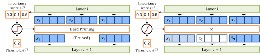
Figure 3. Different pruning strategies for threshold-based token pruning methods. (Left) Hard pruning uses a binary hard mask to select tokens to be pruned. (Right) Soft pruning replaces the binary mask with a differentiable soft mask.

3.1. Background

BERT (Devlin et al., 2018) consists of multiple transformer encoder layers (Vaswani et al., 2017) stacked up together. A basic transformer encoder layer consists of a multi-head attention (MHA) block followed by a point-wise feed-forward (FFN) block, with residual connections around each. Specifically, an MHA consists of $N_{h}$ independently parameterized heads. An attention head $h$ in layer $l$ is parameterized by ${\mathbf{W}}_{k}^{(h,l)},~{}{\mathbf{W}}_{q}^{(h,l)},~{}{\mathbf{W}}_{v}^{(h,l)}\in\mathbb{R}^{d_{h}\times d}$, ${\mathbf{W}}_{o}^{(h,l)}\in\mathbb{R}^{d\times d_{h}}$, where $d_{h}$ is typically set to $d/N_{h}$ and $d$ is the feature dimension. We drop the superscript $l$ for simplicity in the following formula. The MHA measures the pairwise importance of each token on every other token in the input:

(1) $$\text{MHA}(\text{x})=\sum_{h=1}^{N_{h}}\text{Att}_{{\mathbf{W}}_{k,q,v,o}^{(h)}}(\text{x}),$$

where $\text{x}\in\mathbb{R}^{d\times n}$ is the input sequence with the sequence length $n$, and $\text{Att}_{{\mathbf{W}}_{k,q,v,o}}$ is:

(2) $$\text{Att}_{{\mathbf{W}}_{k,q,v,o}}(\text{x}) ={\mathbf{W}}_{o}\sum_{i=1}^{n}{\mathbf{W}}_{v}\text{x}_{i}\text{softmax}(\frac{\text{x}^{T}{\mathbf{W}}_{q}^{T}{\mathbf{W}}_{k}\text{x}_{i}}{\sqrt{d}}),$$

(3) $$\textbf{x}_{\text{MHA}} =\text{LN}\big{(}\text{Att}_{{\mathbf{W}}_{k,q,v,o}}(\text{x})+\text{x}\big{)},$$

where Eq. 3 is the residual connection and the follow up LayerNorm (LN). The output of the MHA is then fed into the FFN block which applies two feed-forward layers to this input:

(4) $$\text{FFN}(\text{x}_{\mathrm{{MHA}}}) =\sigma\big{(}{\mathbf{W}}_{2}({\mathbf{W}}_{1}\text{x}_{\mathrm{{MHA}}}+b_{1})\big{)}+b_{2},$$

(5) $$\textbf{x}_{\mathrm{{out}}} =\text{LN}\big{(}\text{FFN}(\text{x}_{\mathrm{{MHA}}})+\text{x}_{\mathrm{{MHA}}}\big{)},$$

where ${\mathbf{W}}_{1},{\mathbf{W}}_{2},b_{1}$ and $b_{2}$ are the FFN parameters, and $\sigma$ is the activation function (typically GELU for BERT).

3.2. Threshold Token Pruning

Let us denote the attention probability of head $h$ between token x_i and x_j as ${\mathbf{A}}^{(h,l)}$:

(6) $${\mathbf{A}}^{(h,l)}(\text{x}_{i},\text{x}_{j})=\text{softmax}(\frac{\text{x}^{T}{\mathbf{W}}_{q}^{T}{\mathbf{W}}_{k}\text{x}}{\sqrt{d}})_{(i,j)}\in\mathbb{R}.$$

The cost of computational complexity for computing the attention matrix is $\mathcal{O}(d^{2}n+n^{2}d)$, which quadratically scales with sequence length. As such, the attention operation becomes a bottleneck when applied to long sequences. To address this, we apply token pruning which removes unimportant tokens as the input passes through the transformer layers to reduce the sequence length $n$ for later blocks. This is schematically shown in Figure 2 (Left).

For token pruning, we must define a metric to determine unimportant tokens. Following (Goyal et al., 2020; Wang et al., 2020b; Kim and Cho, 2020), we define the importance score of token x_i in layer $l$ as:

(7) $$s^{(l)}(\text{x}_{i})=\frac{1}{N_{h}}\frac{1}{n}\sum_{h=1}^{N_{h}}\sum_{j=1}^{n}{\mathbf{A}}^{(h,l)}(\text{x}_{i},\text{x}_{j}).$$

Intuitively, the attention probability ${\mathbf{A}}^{(h,l)}(\text{x}_{i},\text{x}_{j})$ is interpreted as the normalized amount that all the other tokens x_j attend to token x_i. Token x_i is thus considered important if it receives more attention from all tokens across all heads, which directly leads us to equation 7. The procedure for computing importance scores from attention probabilities is illustrated in Figure 2 (Right).

In (Goyal et al., 2020; Wang et al., 2020b; Kim and Cho, 2020), tokens are ranked by importance score and pruned using a top-$k$ selection strategy. Specially, token x_i is pruned at layer $l$ if its important score $s^{(l)}(\text{x}_{i})$ is smaller than the $k$-largest values of the important score from all the tokens. However, finding the $k$-largest values of the importance score is computationally inefficient without specialized hardware (Wang et al., 2020b); we provide empirical results showing this in Section A.2. Instead, we introduce a new threshold-based token pruning approach in which a token is pruned only if its importance score is below a threshold denoted by $\theta^{(l)}\in\mathbb{R}$. Specifically, we define a pruning strategy by imposing a binary mask $M^{(l)}(\cdot):\{1,\dots,n\}\to\{0,1\}$ which indicates whether a token should be kept or pruned:

(8) $$M^{(l)}(\text{x}_{i})=\begin{cases}1~{}~{}&\text{if }s^{(l)}(\text{x}_{i})>\theta^{(l)},\\ 0~{}~{}&\text{otherwise}.\end{cases}$$

Note that this operation only requires a simple comparison operator without any expensive top-$k$ calculation. Once a token is pruned, it is excluded from calculations in all succeeding layers, thereby gradually reducing computation complexity towards the output layers.

3.3. Learnable Threshold for Token Pruning

A key concern with the method above is how to determine the threshold values for each layer. Not only do threshold values change for different layers, they also vary between different tasks. We address this by making the thresholds (i.e., $\theta$ in Eq. 8) learnable. However, there are several challenges to consider. First, due to the binary nature of $M$ there is no gradient flow for pruned tokens. Second, the $M$ operator is non-differentiable which prevents gradient flow into the thresholds. To address these challenges, we use a soft pruning scheme that simulates the original hard pruning while still propagating gradients to the thresholds as shown in Figure 3.

Soft Pruning Scheme. In the soft pruning scheme, we replace the non-differentiable mask $M^{(l)}$ with a differentiable soft mask using the sigmoid operation $\sigma$:

(9) $$\tilde{M}^{(l)}(\text{x}_{i}) =\sigma\left(\frac{s^{(l)}(\text{x}_{i})-\theta^{(l)}}{T}\right),$$

where $T$ is temperature, and $\theta^{(l)}$ is the learnable threshold value for layer $l$. With sufficiently small temperature $T$, $\tilde{M}^{(l)}(\text{x}_{i})$ will closely approximate the hard masking $M^{(l)}(\text{x}_{i})$ in Eq. 8. In addition, instead of selecting tokens to be pruned or kept based on the hard mask of Eq. 8, we multiply the soft mask to the output activation of layer $l$. That is,

(10) $$\tilde{\text{x}}_{\mathrm{{out}}}^{(l)} =\tilde{M}^{(l)}(\text{x}^{(l)})\cdot\text{x}_{\mathrm{{out}}}^{(l)}$$

(11) $$=\tilde{M}^{(l)}(\text{x}^{(l)})\cdot\mathrm{LN}(\text{FFN}(\text{x}_{\mathrm{{MHA}}}^{(l)})+\text{x}_{\mathrm{{MHA}}}^{(l)}),$$

where $\text{x}_{\mathrm{{MHA}}}^{(l)}$ is the output activation of MHA in layer $l$. If the importance score of token x_i is below the threshold by a large margin, its layer output activation nears zero and thus it has little impact on the succeeding layer. Also, because the token gets a zero importance score in the succeeding layer, i.e., $s^{(l+1)}(\text{x}_{i})=0$, it is likely to be pruned again. Therefore, the soft pruning scheme is nearly identical in behavior to hard pruning, yet its differentiable form allows for backpropagation and gradient-based optimizations to make $\theta$ learnable. After (i) jointly training model parameters and thresholds on downstream tasks with the soft pruning scheme, (ii) we fix the thresholds and binarize the soft mask, and (iii) perform a follow-up fine-tuning of the model parameters. The pseudo-code for this three-step algorithm is given in Algorithm 1. Intuitively, the magnitude of gradient $d\tilde{M}^{(l)}(\text{x}_{i})/d\theta^{(l)}$ is maximized when the importance score $s^{(l)}(\text{x}_{i})$ is close enough to the threshold $\theta^{(l)}$ and becomes near zero elsewhere. Therefore, the threshold can be trained only based on the tokens that are about to be pruned or retained.

Algorithm 1 Three-step Training Procedure for Learnable Threshold Token Pruning

Input: $\mathcal{M}$: model finetuned on target downstream task

Step 1: Apply soft mask to $\mathcal{M}$ and train both the thresholds and model parameters $\triangleright$ Soft Pruning

Step 2: Binarize the mask and fix the thresholds

Step 3: Finetune the model parameters $\triangleright$ Hard Pruning

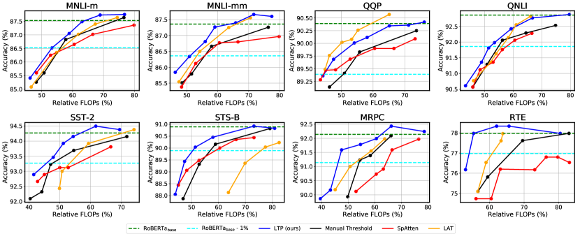
Figure 4. Performance of different pruning methods on GLUE tasks for different token pruning methods across different relative FLOPs, i.e., normalized FLOPs with respect to the the baseline model. Manual threshold assigns linearly raising threshold values for each layer instead of learning them. The performance of the baseline model without token pruning (RoBERTa${}_{\text{base}}$) and the model with 1% performance drop (RoBERTa${}_{\text{base}}$ - 1%) are dotted in horizontal lines for comparison.

Regularization. It is not possible to learn $\theta$ without regularization, as the optimizer generally gets a better loss value if all tokens are present. As such, we add a regularization term to penalize the network if tokens are left unpruned. This is achieved by imposing an L1 loss on the masking operator $\tilde{M}$:

(12) $$\mathcal{L}_{\mathrm{new}}=\mathcal{L}+\lambda\mathcal{L}_{\mathrm{reg}}\enspace\textrm{where}\enspace\mathcal{L}_{\mathrm{reg}}=\frac{1}{L}\sum_{l=1}^{L}||\tilde{M}^{(l)}(\text{x})||_{1}.$$

Here, $\mathcal{L}$ is the original loss function (e.g., cross-entropy loss), and $\lambda$ is the regularization parameter. Larger values of $\lambda$ result in higher pruning ratios. This regularization operator induces an additional gradient to the threshold:

(13) $$\frac{d\mathcal{L}_{\mathrm{reg}}}{d\theta^{(l)}}=\frac{1}{d\theta^{(l)}}||\tilde{M}^{(l)}(\text{x})||_{1}=\sum_{i=1}^{n}\frac{d\tilde{M}^{(l)}(\text{x}_{i})}{d\theta^{(l)}}$$

If there are more tokens near the threshold, then the gradient $d\mathcal{L}_{\mathrm{reg}}/d\theta^{(l)}$ is larger. As a result, the threshold is pushed to a larger value, which prunes more tokens near the threshold boundary.

4. Experiments

4.1. Experiment Setup

We implemented LTP on RoBERTa${}_{\text{base}}$ (Liu et al., 2019) using HuggingFace’s repo and tested on (English) GLUE tasks (Wang et al., 2018) and SQuAD 2.0 (Rajpurkar et al., 2018). For GLUE tasks (Wang et al., 2018), we use 6 tasks for evaluation including sentence similarity (QQP (Iyer et al., 2017), MRPC (Dolan and Brockett, 2005), STS-B (Cer et al., 2017)), sentiment classification (SST-2 (Socher et al., 2013)), textual entailment (RTE (Dagan et al., 2005)) and natural language inference (MNLI (Williams et al., 2017), QNLI (Rajpurkar et al., 2016)). For evaluating the results, we measure classification accuracy and F1 score for MRPC and QQP, Pearson Correlation and Spearman Correlation for STS-B, and classification accuracy for the remaining tasks on validation sets. For the tasks with multiple metrics (i.e., MRPC, QQP, STS-B), we report their average. For SQuAD 2.0 (Rajpurkar et al., 2018), which is a question and answering task, we measure F1 score for evaluating the results.

As mentioned in Section 3.3, the training procedure of LTP consists of two stages: soft pruning that trains both the model parameters and thresholds on downstream tasks, followed by hard pruning that fine-tunes the model parameters with fixed thresholds. We also compare LTP with the current state-of-the-art token pruning methods of SpAtten (Wang et al., 2020b) and LAT (Kim and Cho, 2020) following the implementation details in their papers. See A.1 for the details of the training process. We use PyTorch 1.8 throughout all experiments. For CPU inference speed experiments, we use an Intel Haswell CPU with 3.75GB memory of Google Cloud Platform. For GPU inference speed experiments, we use an AWS p3.2xlarge instance that has a NVIDIA V100 GPU with CUDA 11.1.

An important issue in previous work (Goyal et al., 2020; Kim and Cho, 2020) is that all input sequences for a specific task are padded to the nearest power of 2 from the 99th percentile of the sequence lengths, and then the pruned performance is compared with the padded baseline. This results in exaggerated performance gain over the baseline. For instance, in (Goyal et al., 2020), inputs from the SST-2 dataset are padded to 64, while its average sentence length is 26 (cf. Figure 1). With this approach, one can achieve roughly $2.5\times$ speedup by just removing padding. As such, we avoid any extra padding of input sequences and all speedups and throughputs we report are compared with the unpadded baselines.

Table 1. Detailed performance and efficiency comparison of LTP applied to RoBERTa${}_{\text{base}}$.

Task Accuracy Metric GFLOPs Speedup RoBERTa LTP RoBERTa LTP LTP MNLI-m 87.53 86.53 6.83 3.64 1.88$\times$ MNLI-mm 87.36 86.37 7.15 3.63 1.97$\times$ QQP 90.39 89.69 5.31 2.53 2.10$\times$ QNLI 92.86 91.98 8.94 4.77 1.87$\times$ SST-2 94.27 93.46 4.45 2.13 2.09$\times$ STS-B 90.89 90.03 5.53 2.84 1.95$\times$ MRPC 92.14 91.59 9.33 4.44 2.10$\times$ RTE 77.98 77.98 11.38 6.30 1.81$\times$ SQuAD 2.0 83.04 82.25 32.12 16.99 1.89$\times$

Table 2. Quantiles (Q1/Q2/Q3) and KL divergence of sentence lengths of training and evaluation datasets for GLUE tasks. KL divergence are measured after binning the sentence lengths into 20 bins for RTE, MRPC, and STS-B and 50 bins for the others.

Task Quantiles (train) Quantiles (eval) KL Div. MNLI-m 27/38/50 26/37/50 0.0055 MNLI-mm 27/38/50 29/39/51 0.0042 QQP 23/28/36 23/28/36 0.0006 QNLI 39/48/59 39/49/61 0.0092 SST-2 7/11/19 18/25/33 1.2250 STS-B 20/24/32 21/29/41 0.0925 MRPC 45/54/63 45/54/64 0.0033 RTE 44/57/86 42/54/78 0.0261

4.2. Performance Evaluation

Table 1 lists the accuracy and GFLOPs for LTP. We select a model for each downstream task that achieves the smallest GFLOPs while constraining the accuracy degradation from the baseline (RoBERTa${}_{\text{base}}$) to be at most 1%. Using our method, sequence lengths in each layer can vary across different input sentences. Therefore, we report the averaged GFLOPs of processing all input sentences in the development set. As shown in the table, our method achieves speedup of 1.96$\times$ on average and up to 2.10$\times$ within 1% accuracy degradation.

Figure 4 plots the accuracy of LTP (blue lines) as well as the prior pruning methods (red lines for SpAtten and orange lines for LAT) with different FLOPs on GLUE tasks. LTP consistently outperforms SpAtten for all tasks with up to ~2% higher accuracy under the same amount of FLOPs. Compared with LAT, LTP outperforms for all tasks except for QQP with up to ~2.5% higher accuracy for the same target FLOPs. For QQP alone, LTP achieves at most ~0.2% lower accuracy than LTP.

An important observation is that for SST-2 and STS-B where LTP (ours) outperforms LAT with large margins, the sequence length varies greatly from the training dataset to the evaluation dataset as can be seen from the large KL-divergence in Table 2 and Figure 1 (b, c). On the other hand, for QQP, the only dataset that LAT slightly outperforms LTP (ours), the sequence length distribution of the training dataset is almost identical to that of the evaluation dataset as can be seen from the small KL-divergence in Table 2 and Figure 2 (a). This observation supports our claim in Section 1 and 2: LTP is robust to sequence length variations as it does not fix the pruning configuration unlike other methods using a single pruning configuration regardless of the input sequence length. This is important in practice because the sequence lengths during inference do not always follow the sequence length distribution of the training dataset as in SST-2 and STS-B. We make a further discussion in Section 4.3.

For SQuAD 2.0, we have similar results to GLUE. As can be seen in Table 1 and Figure 5 (Left), we obtain nearly identical F1 score to baseline at 0.58 relative FLOPs, and 1.89$\times$ speedup with less than 1% drop of F1 score. The SQuAD 2.0 dataset is divided into two subsets: the subset of examples where the answer to the question is included in the context text, and the subset that has no answer. In Figure 5 (Right), we further plot the results on each subset of the dataset (black and red for the one with and without answers, respectively). We see that the F1 score decreases for the subset with answers and increases for the subset without answers as we decrease the relative FLOPs. This is to be expected as the question answering head will predict no answer if the start and end points of the answer within the context cannot be determined due to high token pruning ratios. Thus, a careful setting of $\lambda$ in Eq. 12 is necessary to balance the accuracy between the two subsets.

At last, we also highlight that LTP has an additional gain over the prior top-$k$ based approaches by avoiding computationally inefficient top-$k$ operations as further discussed in Section A.2.

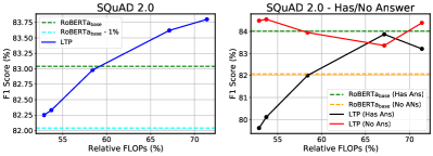
Figure 5. (Left) Performance of LTP on SQuAD 2.0 across different relative FLOPs with respect to the the baseline model on the full validation set. (Right) Performance of LTP on the subsets of the validation set, one with answers (Has Ans, black) and the other without (No Ans, red). The performance of the baseline model without token pruning (RoBERTa${}_{\text{base}}$) and the model with 1% performance drop (RoBERTa${}_{\text{base}}$ - 1%) are dotted in horizontal lines for comparison.

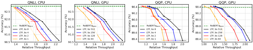
Figure 6. Relative throughput of LTP with respect to the baseline without token pruning (RoBERTa${}_{\text{base}}$) with different batch sizes on Intel Haswell CPU and NVIDIA V100 GPU. The performance of RoBERTa${}_{\text{base}}$ are dotted in horizontal lines.

4.3. Robustness to Sequence Length Variation

In Section 4.2, we claim that LTP is more robust against sequence length variations from training time to evaluation time. Here, we make a more systematic analysis on this. Ideally, performance should be independent of sequence length. To quantitatively test the robustness of pruning methods against sequence length variations, we train LTP and LAT on QNLI and QQP, but only using the training examples whose sequence lengths are below the median length of the evaluation dataset. We then evaluate the resulting models using the evaluation examples with sequence lengths (i) below the median (~Q2), (ii) between the median and the third quantile (Q2~Q3), and (iii) above the third quantile (Q3~) of the evaluation dataset. To make a fair comparison, we choose models from LTP and LAT that require similar FLOPs on ~Q2.

The results are listed in Table 3. LTP consistently achieves better accuracy and FLOPs over different sequence lengths, even with those that are significantly longer than the training sequences. On the contrary, LAT shows significant accuracy degradation as longer sequences are over-pruned, which can be seen from the significant FLOPs reduction. In particular, LTP outperforms LAT by up to 16.44% and 9.20% on QNLI and QQP for the Q3~ evaluation dataset.

Table 3. LTP and LAT trained with the sequences shorter than the median length, and evaluated with the sequences shorther than the median (~Q2), between the median and the third quantile (Q2~Q3), and longer than the third quantile (Q3~) of the evaluation dataset. FLOPs are relative FLOPs (%) with respect to RoBERTa_base.

Task QNLI QQP ~Q2 Q2~Q3 Q3~ ~Q2 Q2~Q3 Q3~ LTP Acc. 91.21 90.02 91.81 89.42 89.51 91.37 (ours) FLOPs 55.89 55.60 56.02 55.18 56.29 58.01 LAT Acc. 90.87 86.12 75.37 89.20 87.27 82.17 FLOPs 56.21 46.55 35.89 55.17 46.61 34.14 Diff. Acc. +0.34 +3.90 +16.44 +0.22 +2.24 +9.20

4.4. Ablation Studies

Instead of learning thresholds, we can set them manually. Because manually searching over the exponential search space is intractable, we add a constraint to the search space by assigning linearly rising threshold values for each layer, similar to how SpAtten (Wang et al., 2020b) assigns the token retain ratios: given the threshold of the final layer $\theta^{(L)}$, the threshold for layer $l$ is set as $\theta^{(L)}l/{L}$. We plot the accuracy and FLOPs of the manual threshold approach in Figure 4 as black lines. While this approach exhibits decent results on all downstream tasks, the learned thresholds consistently outperform the manual thresholds under the same FLOPs. This provides empirical evidence for the effectiveness of our threshold learning method.

4.5. Direct Throughput Measurement on Hardware

We directly measure throughputs on real hardware by deploying LTP on a NVIDIA V100 GPU and a Intel Haswell CPU. For inference, we completely remove the pruned tokens and rearrange the retained tokens into a blank-free sequence to have a latency gain. One consequence of adaptive pruning, however, is that each sequence will end up with a different pruning pattern and sequence length. As such, a naive hardware implementation of batched inference may require padding all the sequences in a batch to ensure that they all have the same length (i.e., the maximum sequence length in the batch), which results in a significant portion of computation being wasted to process padding tokens. To avoid this, we use NVIDIA’s Faster Transformer for GPU implementation that requires large batch sizes. This framework dynamically removes and inserts padding tokens during inference so that most of the transformer operations effectively skip processing padding tokens. This enables fast inference even with irregular pruning lengths of individual sequences. For the CPU implementation, we find naive batching (i.e., padding sequences to the maximum sentence length) enough for good throughput.

The measured throughput results are shown in Figure 6 for different batch sizes. For all experiments, relative throughput is evaluated 3 times on the randomly shuffled datasets. LTP achieves up to $\sim$1.9$\times$ and $\sim$2.0$\times$ thoughput improvement for QNLI and QQP on both CPU and GPU, as compared to the baseline. This is similar to the theoretical speedup inferred from the FLOPs reduction reported in Table 1. Importantly, the speedup of LTP increases with larger batch sizes on both CPU and GPU, proving effectiveness of LTP on batched cases.

4.6. LTP with Quantization and Knowledge Distillation

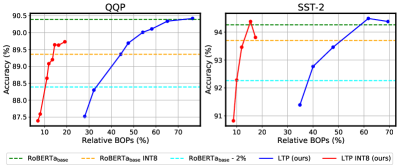
Figure 7. Accuracy and relative BOPs of the FP16 baselines and INT8 LTP models on QQP and SST-2 datasets. Note that FP16 unpruned RoBERTa${}_{\text{base}}$ is used as the baseline. Thus, INT8 quantization of the models translates to $4\times$ reduction in relative BOPs.

Here, we show that our token-level pruning method is compatible with other compression methods. In particular, we perform compression experiments by combining LTP with quantization and knowledge distillation (Hinton et al., 2015) together. For quantization, we use the static uniform symmetric integer quantization method (Gholami et al., 2021), which is easy to deploy in commodity hardware with minimal run-time overhead. All the model parameters are quantized to 8-bit integers, except for those of the embedding layer whose bit-width does not affect the inference speed. Afterwards, we apply knowledge distillation that helps recover accuracy for high compression ratios. We set the baseline RoBERTa${}_{\text{base}}$ model as the teacher and the quantized LTP model as the student. We then distill knowledge from the teacher model into the student model through a knowledge distillation loss that matches the output logits of the classification layer and the output representations of the embedding layer in the teacher model to the counterparts in the student model. The training objective is a convex combination of the original loss and the knowledge distillation loss. As shown in Figure 7, we achieve up to 10$\times$ reduction in bit operations (BOPs) with less than $2\%$ accuracy degradation as compared to FP16 RoBERTa${}_{\text{base}}$ by combining quantization and knowledge distillation. The results empirically show the effectiveness of LTP with other compression methods.

5. Conclusions

In this work, we present Learned Token Pruning (LTP), a fully automated token pruning framework for transformers. LTP only requires comparison of token importance scores with threshold values to determine unimportant tokens, thus adding minimal complexity over the original transformer inference. Importantly, the threshold values are learned for each layer during training through a differentiable soft binarized mask that enables backpropagation of gradients to the threshold values. Compared to the state-of-the-art token pruning methods, LTP outperforms by up to ~2.5% accuracy with the same amount of FLOPs. Extensive experiments on GLUE and SQuAD show the effectiveness of LTP, as it achieves up to 2.10$\times$ FLOPs reduction over the baseline model within only 1% of accuracy degradation. Our preliminary (and not highly optimized) implementation shows up to 1.9$\times$ and 2.0$\times$ throughput improvement on an Intel Haswell CPU and a NVIDIA V100 GPU. Furthermore, LTP exhibits significantly better robustness and consistency over different input sequence lengths.

Appendix A Appendix

A.1. Training Details

The training procedure of LTP consists of two separate stages: soft pruning followed by hard pruning. For soft pruning, we train both the model parameters and the thresholds on downstream tasks for 1 to 10 epochs, depending on the dataset size. We find it effective to initialize the thresholds with linearly rising values as described in 4.4 with a fixed threshold of the final layer. We search the optimal temperature $T$ in a search space of {1, 2, 5, 10, 20}e-4 and vary $\lambda$ from 0.001 to 0.4 to control the number of tokens to be pruned (and thus the FLOPs) for all experiments. We then fix the thresholds and perform an additional training with the hard pruning to fine-tune the model parameters only. More detailed hyperparameter settings are listed in Table A.1 for GLUE and SQuAD 2.0.

SpAtten is trained based on the implementation details in the paper: the first three layers retain all tokens and the remaining layers are assigned with linearly decaying token retain ratio until it reaches the final token retain ratio at the last layer. We vary the final token retain ratio from 1.0 to -1.0 (prune all tokens for non-positive retain ratios) to control the FLOPs of SpAtten. For both LTP and SpAtten, we use learning rate of {0.5, 1, 2}e-5, except for the soft pruning stage of LTP where we use 2e-5. We follow the optimizer setting in RoBERTa (Liu et al., 2019) and use batch size of 64 for all experiments.

LAT is trained using the same hyperparameter and optimizer setting in the paper except for the length drop probabilities: for more extensive search on more aggressive pruning configurations, we used 0.25, 0.3, 0.35, and 0.4 for the length drop probability instead of 0.2 in the original setting.

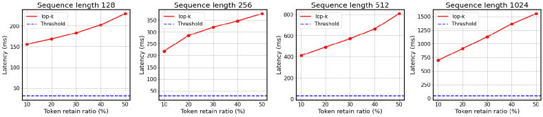
Figure A.1. Wall-clock latency comparison between top-$k$ operation and threshold operation on an Intel Haswell CPU for different sequence length across various token retain ratios. Note that the latency of a threshold operation is independent of sequence length.

A.2. Computation Efficiency Comparison

Here we compare the efficiency of top-$k$ versus threshold operation. To do this, we use a batch size of 32 and average the latency over 1000 independent runs. For each sequence length, we test over five different token retain ratios from 10% to 50% (e.g., 10% token retain ratio is the case where we select top-$k$ 10% of tokens from the input sequence).

With the above setting, we directly measure the latency of these two operations on an Intel Haswell CPU, and report the results in Figure A.1. For top-$k$ operation, there is a noticeable increase in latency when token retain ratios and sequence lengths become larger whereas this is not an issue for our threshold pruning method as it only requires a comparison operation. More importantly, top-$k$ operation incurs a huge latency overhead that is up to 7.4$\times$ and 33.4$\times$ slower than threshold operation for sequence length of 128 and 1024, respectively.

Table A.1. Detailed hyperparameters for LTP training.

Stage Hyperparam GLUE SQuAD 2.0 Soft pruning epochs 1 - 10 1 learning rate 2e-5 2e-5 $T$ $\{$1, 2, 5, 10, 20$\}$e-4 $\{$1, 10$\}$e-4 $\lambda$ 0.001 - 0.2 0.001 - 0.4 init. final thres. 0.01 0.003 Hard epochs 10 5 pruning lr {0.5, 1, 2}e-5 {0.5, 1, 2}e-5

A.3. Discussion

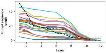
(a) SST-2

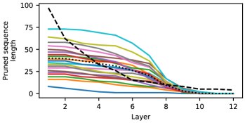
(b) MNLI-m

Figure A.2. Sample trajectories of pruned sequence length as the sequences are passed through model layers. For LTP, 20 samples were evenly selected from the sets after sorting by initial sequence length. (a) SST-2. (b) MNLI-m. The mean sequence length for LTP is shown by a black dotted line, and the LAT baseline is shown by a black dashed line. Parameters were selected so as to provide a 1% drop in accuracy from baseline for both methods.

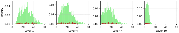
(a) SST2

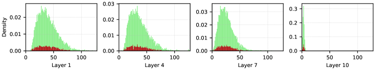
(b) MNLI-m

Figure A.3. Histogram of pruned sequence length (x-axis) as the input sequence is processed through different transformer blocks. y-axis shows the relative count of sentences with the particular sequence length in x-axis. Green denotes input sequences that are correctly classified, and red denotes incorrect classifications.

A.3.1. Example Sequence Length Trajectories

Figure A.2 shows how the pruned sequence length decreases for input sequences of varying lengths. For LAT, the token pruning configuration is fixed for all sequences in the dataset. In LTP, token pruning can be more or less aggressive depending on the sequence content and the number of important tokens in the sequence. On average, LTP calculates 25.86% fewer tokens per layer than LAT for MNLI-m and 12.08% fewer tokens for SST-2. For both LTP and LAT, the model has been trained to produce a 1% drop in accuracy compared to baseline.

A.3.2. Unbiased Token Pruning for Various Sequence Length

Figure A.3 shows the distributions of initial sequence lengths for sequences that are correctly classified and for sequences that are not. We see that for multiple tasks, there is no significant correlation between the length of the sequence and the accuracy of the pruned models. Importantly, this suggests that our method is not biased towards being more accurate on longer or shorter sequences.

A.4. Comparison with TR-BERT on GLUE

Unlike LAT and SpAtten, TR-BERT (Ye et al., 2021) does not report results on the GLUE benchmark tasks described in the paper. We attempted to run TR-BERT on the GLUE tasks using the TR-BERT repo, but were unable to get the algorithm to converge to a high accuracy, despite varying the learning rate between 1e-6 and 1e-3 and the value of $\alpha$, the parameter that defines the length penalty, over the search space of $\{0.01,0.05,0.1,0.5,1,2,5\}$. We also varied the number of training epochs based on the number of examples in each task’s training set. The authors of TR-BERT note the convergence difficulties of RL learning while describing the algorithm in their paper.

References

- (1)
- Bai et al. (2020) Haoli Bai, Wei Zhang, Lu Hou, Lifeng Shang, Jing Jin, Xin Jiang, Qun Liu, Michael Lyu, and Irwin King. 2020. BinaryBERT: Pushing the Limit of BERT Quantization. arXiv preprint arXiv:2012.15701 (2020).
- Bhandare et al. (2019) Aishwarya Bhandare, Vamsi Sripathi, Deepthi Karkada, Vivek Menon, Sun Choi, Kushal Datta, and Vikram Saletore. 2019. Efficient 8-bit quantization of transformer neural machine language translation model. arXiv preprint arXiv:1906.00532 (2019).
- Cer et al. (2017) Daniel Cer, Mona Diab, Eneko Agirre, Inigo Lopez-Gazpio, and Lucia Specia. 2017. Semeval-2017 task 1: Semantic textual similarity-multilingual and cross-lingual focused evaluation. arXiv preprint arXiv:1708.00055 (2017).
- Chen et al. (2020) Tianlong Chen, Jonathan Frankle, Shiyu Chang, Sijia Liu, Yang Zhang, Zhangyang Wang, and Michael Carbin. 2020. The lottery ticket hypothesis for pre-trained BERT networks. arXiv preprint arXiv:2007.12223 (2020).
- Child et al. (2019) Rewon Child, Scott Gray, Alec Radford, and Ilya Sutskever. 2019. Generating long sequences with sparse transformers. arXiv preprint arXiv:1904.10509 (2019).
- Dagan et al. (2005) Ido Dagan, Oren Glickman, and Bernardo Magnini. 2005. The PASCAL recognising textual entailment challenge. In Machine Learning Challenges Workshop. Springer, 177–190.
- Devlin et al. (2018) Jacob Devlin, Ming-Wei Chang, Kenton Lee, and Kristina Toutanova. 2018. Bert: Pre-training of deep bidirectional transformers for language understanding. arXiv preprint arXiv:1810.04805 (2018).
- Dolan and Brockett (2005) William B Dolan and Chris Brockett. 2005. Automatically constructing a corpus of sentential paraphrases. In Proceedings of the Third International Workshop on Paraphrasing (IWP2005).
- Fan et al. (2019) Angela Fan, Edouard Grave, and Armand Joulin. 2019. Reducing transformer depth on demand with structured dropout. arXiv preprint arXiv:1909.11556 (2019).
- Fan et al. (2020) Angela Fan, Pierre Stock, Benjamin Graham, Edouard Grave, Rémi Gribonval, Hervé Jégou, and Armand Joulin. 2020. Training with quantization noise for extreme model compression. arXiv e-prints (2020), arXiv–2004.
- Frankle and Carbin (2018) Jonathan Frankle and Michael Carbin. 2018. The lottery ticket hypothesis: Finding sparse, trainable neural networks. arXiv preprint arXiv:1803.03635 (2018).
- Gholami et al. (2021) Amir Gholami, Sehoon Kim, Zhen Dong, Zhewei Yao, Michael W Mahoney, and Kurt Keutzer. 2021. A survey of quantization methods for efficient neural network inference. arXiv preprint arXiv:2103.13630 (2021).
- Goyal et al. (2020) Saurabh Goyal, Anamitra Roy Choudhury, Saurabh Raje, Venkatesan Chakaravarthy, Yogish Sabharwal, and Ashish Verma. 2020. Power-bert: Accelerating bert inference via progressive word-vector elimination. In International Conference on Machine Learning. PMLR, 3690–3699.
- Hinton et al. (2015) Geoffrey Hinton, Oriol Vinyals, and Jeff Dean. 2015. Distilling the knowledge in a neural network. arXiv preprint arXiv:1503.02531 (2015).
- Hou et al. (2020) Lu Hou, Zhiqi Huang, Lifeng Shang, Xin Jiang, Xiao Chen, and Qun Liu. 2020. Dynabert: Dynamic bert with adaptive width and depth. arXiv preprint arXiv:2004.04037 (2020).
- Iandola et al. (2020) Forrest N Iandola, Albert E Shaw, Ravi Krishna, and Kurt W Keutzer. 2020. SqueezeBERT: What can computer vision teach NLP about efficient neural networks? arXiv preprint arXiv:2006.11316 (2020).
- Iyer et al. (2017) Shankar Iyer, Nikhil Dandekar, and Kornl Csernai. 2017. First Quora Dataset Release: Question Pairs.(2017). URL https://data. quora. com/First-Quora-Dataset-Release-Question-Pairs (2017).
- Jiao et al. (2019) Xiaoqi Jiao, Yichun Yin, Lifeng Shang, Xin Jiang, Xiao Chen, Linlin Li, Fang Wang, and Qun Liu. 2019. Tinybert: Distilling bert for natural language understanding. arXiv preprint arXiv:1909.10351 (2019).
- Katharopoulos et al. (2020) Angelos Katharopoulos, Apoorv Vyas, Nikolaos Pappas, and François Fleuret. 2020. Transformers are rnns: Fast autoregressive transformers with linear attention. In International Conference on Machine Learning. PMLR, 5156–5165.
- Khetan and Karnin (2020) Ashish Khetan and Zohar Karnin. 2020. schubert: Optimizing elements of bert. arXiv preprint arXiv:2005.06628 (2020).
- Kim and Cho (2020) Gyuwan Kim and Kyunghyun Cho. 2020. Length-Adaptive Transformer: Train Once with Length Drop, Use Anytime with Search. arXiv preprint arXiv:2010.07003 (2020).
- Kim et al. (2021) Sehoon Kim, Amir Gholami, Zhewei Yao, Michael W Mahoney, and Kurt Keutzer. 2021. I-BERT: Integer-only BERT Quantization. International conference on machine learning (2021).
- Kitaev et al. (2020) Nikita Kitaev, Łukasz Kaiser, and Anselm Levskaya. 2020. Reformer: The efficient transformer. arXiv preprint arXiv:2001.04451 (2020).
- Lagunas et al. (2021) François Lagunas, Ella Charlaix, Victor Sanh, and Alexander M Rush. 2021. Block pruning for faster transformers. arXiv preprint arXiv:2109.04838 (2021).
- Lan et al. (2019) Zhenzhong Lan, Mingda Chen, Sebastian Goodman, Kevin Gimpel, Piyush Sharma, and Radu Soricut. 2019. Albert: A lite bert for self-supervised learning of language representations. arXiv preprint arXiv:1909.11942 (2019).
- Li et al. (2020) Bingbing Li, Zhenglun Kong, Tianyun Zhang, Ji Li, Zhengang Li, Hang Liu, and Caiwen Ding. 2020. Efficient transformer-based large scale language representations using hardware-friendly block structured pruning. arXiv preprint arXiv:2009.08065 (2020).
- Lin et al. (2020) Zi Lin, Jeremiah Zhe Liu, Zi Yang, Nan Hua, and Dan Roth. 2020. Pruning Redundant Mappings in Transformer Models via Spectral-Normalized Identity Prior. arXiv preprint arXiv:2010.01791 (2020).
- Liu et al. (2019) Yinhan Liu, Myle Ott, Naman Goyal, Jingfei Du, Mandar Joshi, Danqi Chen, Omer Levy, Mike Lewis, Luke Zettlemoyer, and Veselin Stoyanov. 2019. RoBERTa: A robustly optimized bert pretraining approach. arXiv preprint arXiv:1907.11692 (2019).
- Liu et al. (2021) Zejian Liu, Fanrong Li, Gang Li, and Jian Cheng. 2021. EBERT: Efficient BERT Inference with Dynamic Structured Pruning. In Findings of the Association for Computational Linguistics: ACL-IJCNLP 2021. 4814–4823.
- Michel et al. (2019) Paul Michel, Omer Levy, and Graham Neubig. 2019. Are sixteen heads really better than one? arXiv preprint arXiv:1905.10650 (2019).
- Prasanna et al. (2020) Sai Prasanna, Anna Rogers, and Anna Rumshisky. 2020. When BERT plays the lottery, all tickets are winning. arXiv preprint arXiv:2005.00561 (2020).
- Press et al. (2021) Ofir Press, Noah A Smith, and Mike Lewis. 2021. Train Short, Test Long: Attention with Linear Biases Enables Input Length Extrapolation. arXiv preprint arXiv:2108.12409 (2021).
- Rajpurkar et al. (2018) Pranav Rajpurkar, Robin Jia, and Percy Liang. 2018. Know what you don’t know: Unanswerable questions for SQuAD. arXiv preprint arXiv:1806.03822 (2018).
- Rajpurkar et al. (2016) Pranav Rajpurkar, Jian Zhang, Konstantin Lopyrev, and Percy Liang. 2016. SQuAD: 100,000+ questions for machine comprehension of text. arXiv preprint arXiv:1606.05250 (2016).
- Roy et al. (2021) Aurko Roy, Mohammad Saffar, Ashish Vaswani, and David Grangier. 2021. Efficient content-based sparse attention with routing transformers. Transactions of the Association for Computational Linguistics 9 (2021), 53–68.
- Sajjad et al. (2020) Hassan Sajjad, Fahim Dalvi, Nadir Durrani, and Preslav Nakov. 2020. On the Effect of Dropping Layers of Pre-trained Transformer Models. arXiv preprint arXiv:2004.03844 (2020).
- Sanh et al. (2019) Victor Sanh, Lysandre Debut, Julien Chaumond, and Thomas Wolf. 2019. DistilBERT, a distilled version of BERT: smaller, faster, cheaper and lighter. arXiv preprint arXiv:1910.01108 (2019).
- Sanh et al. (2020) Victor Sanh, Thomas Wolf, and Alexander M Rush. 2020. Movement pruning: Adaptive sparsity by fine-tuning. arXiv preprint arXiv:2005.07683 (2020).
- Shen et al. (2020) Sheng Shen, Zhen Dong, Jiayu Ye, Linjian Ma, Zhewei Yao, Amir Gholami, Michael W Mahoney, and Kurt Keutzer. 2020. Q-BERT: Hessian Based Ultra Low Precision Quantization of BERT.. In AAAI. 8815–8821.
- Socher et al. (2013) Richard Socher, Alex Perelygin, Jean Wu, Jason Chuang, Christopher D Manning, Andrew Y Ng, and Christopher Potts. 2013. Recursive deep models for semantic compositionality over a sentiment treebank. In Proceedings of the 2013 conference on empirical methods in natural language processing. 1631–1642.
- Sun et al. (2019) Siqi Sun, Yu Cheng, Zhe Gan, and Jingjing Liu. 2019. Patient knowledge distillation for bert model compression. arXiv preprint arXiv:1908.09355 (2019).
- Sun et al. (2020) Zhiqing Sun, Hongkun Yu, Xiaodan Song, Renjie Liu, Yiming Yang, and Denny Zhou. 2020. Mobilebert: a compact task-agnostic bert for resource-limited devices. arXiv preprint arXiv:2004.02984 (2020).
- Tang et al. (2019) Raphael Tang, Yao Lu, Linqing Liu, Lili Mou, Olga Vechtomova, and Jimmy Lin. 2019. Distilling task-specific knowledge from BERT into simple neural networks. arXiv preprint arXiv:1903.12136 (2019).
- Tay et al. (2020) Yi Tay, Dara Bahri, Liu Yang, Donald Metzler, and Da-Cheng Juan. 2020. Sparse sinkhorn attention. In International Conference on Machine Learning. PMLR, 9438–9447.
- Vaswani et al. (2017) Ashish Vaswani, Noam Shazeer, Niki Parmar, Jakob Uszkoreit, Llion Jones, Aidan N Gomez, Łukasz Kaiser, and Illia Polosukhin. 2017. Attention is all you need. In Advances in neural information processing systems. 5998–6008.
- Voita et al. (2019) Elena Voita, David Talbot, Fedor Moiseev, Rico Sennrich, and Ivan Titov. 2019. Analyzing multi-head self-attention: Specialized heads do the heavy lifting, the rest can be pruned. arXiv preprint arXiv:1905.09418 (2019).
- Vyas et al. (2020) Apoorv Vyas, Angelos Katharopoulos, and François Fleuret. 2020. Fast transformers with clustered attention. Advances in Neural Information Processing Systems 33 (2020).
- Wang et al. (2018) Alex Wang, Amanpreet Singh, Julian Michael, Felix Hill, Omer Levy, and Samuel R Bowman. 2018. GLUE: A multi-task benchmark and analysis platform for natural language understanding. arXiv preprint arXiv:1804.07461 (2018).
- Wang et al. (2020b) Hanrui Wang, Zhekai Zhang, and Song Han. 2020b. SpAtten: Efficient Sparse Attention Architecture with Cascade Token and Head Pruning. arXiv preprint arXiv:2012.09852 (2020).
- Wang et al. (2020a) Sinong Wang, Belinda Li, Madian Khabsa, Han Fang, and Hao Ma. 2020a. Linformer: Self-Attention with Linear Complexity. arXiv preprint arXiv:2006.04768 (2020).
- Wang et al. (2019) Ziheng Wang, Jeremy Wohlwend, and Tao Lei. 2019. Structured pruning of large language models. arXiv preprint arXiv:1910.04732 (2019).
- Williams et al. (2017) Adina Williams, Nikita Nangia, and Samuel R Bowman. 2017. A broad-coverage challenge corpus for sentence understanding through inference. arXiv preprint arXiv:1704.05426 (2017).
- Yao et al. (2021) Zhewei Yao, Linjian Ma, Sheng Shen, Kurt Keutzer, and Michael W Mahoney. 2021. MLPruning: A Multilevel Structured Pruning Framework for Transformer-based Models. arXiv preprint arXiv:2105.14636 (2021).
- Ye et al. (2021) Deming Ye, Yankai Lin, Yufei Huang, and Maosong Sun. 2021. TR-BERT: Dynamic Token Reduction for Accelerating BERT Inference. arXiv preprint arXiv:2105.11618 (2021).
- Zadeh et al. (2020) Ali Hadi Zadeh, Isak Edo, Omar Mohamed Awad, and Andreas Moshovos. 2020. Gobo: Quantizing attention-based nlp models for low latency and energy efficient inference. In 2020 53rd Annual IEEE/ACM International Symposium on Microarchitecture (MICRO). IEEE, 811–824.
- Zafrir et al. (2019) Ofir Zafrir, Guy Boudoukh, Peter Izsak, and Moshe Wasserblat. 2019. Q8BERT: Quantized 8bit bert. arXiv preprint arXiv:1910.06188 (2019).
- Zaheer et al. (2020) Manzil Zaheer, Guru Guruganesh, Avinava Dubey, Joshua Ainslie, Chris Alberti, Santiago Ontanon, Philip Pham, Anirudh Ravula, Qifan Wang, Li Yang, et al. 2020. Big bird: Transformers for longer sequences. arXiv preprint arXiv:2007.14062 (2020).
- Zhang et al. (2020) Wei Zhang, Lu Hou, Yichun Yin, Lifeng Shang, Xiao Chen, Xin Jiang, and Qun Liu. 2020. Ternarybert: Distillation-aware ultra-low bit bert. arXiv preprint arXiv:2009.12812 (2020).
- Zhao et al. (2020) Mengjie Zhao, Tao Lin, Fei Mi, Martin Jaggi, and Hinrich Schütze. 2020. Masking as an efficient alternative to finetuning for pretrained language models. arXiv preprint arXiv:2004.12406 (2020).