Spectra of new graph operations based on central graph

Abstract

In this paper, we introduce central vertex corona, central edge corona, and central edge neighborhood corona of graphs using central graph. Also, we determine their adjacency spectrum, Laplacian spectrum and signless Laplacian spectrum. From our results, it is possible to obtain infinitely many pairs of adjacency (respectively, Laplacian and signless Laplacian) cospectral graphs. As an application, we calculate the number of spanning trees and the Kirchhoff index of the resulting graphs.

AMS classification: 05C50

Keywords: Adjacency spectrum, Laplacian spectrum, signless Laplacian spectrum, corona of graphs, central graph.

1 Introduction

In this paper, we consider only simple connected graphs. Let $G=(V(G),E(G))$ be a graph with vertex set $V(G)=\{v_{1},v_{2},...,v_{n}\}$ and edge set $E(G)=\{e_{1},e_{2},...,e_{m}\}$, and let $d_{i}$ be the degree of the vertex $v_{i},v_{i}\in V(G).$ The adjacency matrix $A(G)$ of the graph $G$ is a square symmetric matrix of order $n$ whose $(i,j)^{th}$ entry is equal to unity if the vertices $v_{i}$ and $v_{j}$ are adjacent, and is equal to zero otherwise. The Laplacian matrix of $G$, denoted by $L(G)$ is defined as $L(G)=D(G)-A(G)$ and the signless Laplacian matrix of $G$, denoted by $Q(G)$ is defined as $Q(G)=D(G)+A(G)$, where $D(G)$ is the diagonal matrix whose entries are the degrees of the vertices of $G$. The characteristic polynomial of the $n\times n$ matrix $M$ of $G$ is defined as $f(M,x)=|xI_{n}-M|$, where $I_{n}$ is identity matrix of order $n$. The matrices $A(G),L(G)$ and $Q(G)$ are real symmetric matrices, its eigenvalues are real. Denote the eigenvalues of $A(G),L(G)$ and $Q(G)$ by $\lambda_{1}(G)\geqslant\lambda_{2}(G)\geqslant...\geqslant\lambda_{n}(G),0=\mu_{1}(G)<\mu_{2}(G)\leq...\leq\mu_{n}(G)$ and $\gamma_{1}(G)\geq\gamma_{2}(G)\geq...\geq\gamma_{n}(G)$, respectively. The set of all eigenvalues of $A(G)$ (respectively, $L(G)$, Q(G)) together with their multiplicities are called $A$-spectrum (respectively, $L$-spectrum, $Q$-spectrum) of $G$. Two non isomorphic graphs are said to be $A$-cospectral (respectively, $L$-cospectral, $Q$-cospectral), if they have the same $A$-spectrum (respectively, $L$-spectrum, $Q$-spectrum). Otherwise, they are non $A$-cospectral (respectively, non $L$-cospectral, non $Q$-cospectral) graphs. Let $G$ be a connected graph on $n$ vertices, then the number of spanning trees of $G$ is $t(G)=\frac{\mu_{2}(G)\cdot\mu_{3}(G)...\mu_{n}(G)}{n}$[1]. In 1993, Klein and Randić [2] introduced the resistance distance $r_{i,j}^{*}$ between two vertices $v_{i}$ and $v_{j}$ in $G$ and is defined as the effective resistance between them when unit resistors are distributed on every edge of G. The Kirchhoff index [3] of a connected graph $G$ is defined as

$$Kf(G)=\sum_{i<j}r_{i,j}^{*},$$

where $r_{i,j}^{*}$ denotes the resistance distance between vertices $v_{i}$ and $v_{j}$ in $G$. In [4, 5], the authors proved that the Kirchhoff index of a graph $G$ is

$$Kf(G)=n\displaystyle\sum_{i=2}^{n}\frac{1}{\mu_{i}(G)}.$$

In literature, there are many graph operations like, complement, disjoint union, join, cartesian product, direct product, strong product, lexicographic product, corona, edge corona, neighbourhood corona etc. The corona of two graphs first introduced by F.Harary and R.Frucht in [6]. Recently, several variants of corona product of two graphs have been introduced and their spectra are computed. In [7], Liu and Lu introduced subdivision-vertex and subdivision-edge neighbourhood corona of two graphs and provided a complete description of their spectra. In [8], Lan and Zhou introduced $R$-vertex corona, $R$-edge corona, $R$-vertex neighborhood corona and $R$-edge neighborhood corona, and studied their spectra. Recently in [9, 10], Adiga et.al introduced duplication corona, duplication neighborhood corona, duplication edge corona, N-vertex corona and N-edge corona of two regular graphs. Motivated by the above works, we define three new graph operations based on central graph.

The Kronecker product $A\otimes B$ of two matrices $A=(a_{i,j})_{m\times n}$ and $B=(b_{i,j})_{p\times q}$ is the $mp\times nq$ matrix obtained from A by replacing each entry $a_{i,j}$ by $a_{i,j}B$. For matrices A,B,C and D such that products AC and BD exist then $(A\otimes B)(C\otimes D)=AC\otimes BD.$ Also, if $A$ and $B$ are invertible matrices, then $(A\otimes B)^{-1}=A^{-1}\otimes B^{-1}$, $(A\otimes B)^{T}=A^{T}\otimes B^{T}$. If A and B are $n\times n$ and $p\times p$ matrices respectively, then $det(A\otimes B)=(detA)^{p}(detB)^{n}$[11]. The incidence matrix of a graph $G$, $I(G)$ is the $n\times m$ matrix whose $(i,j)^{th}$ entry is 1 if $v_{i}$ is incident to $e_{j}$ and 0 otherwise. It is known [12] that, $I(G)I(G)^{T}=A(G)+D(G)$ and if $G$ is an $r$-regular graph, then $I(G)I(G)^{T}=A(G)+rI_{n}$. The complement $\bar{G}$ of a graph $G$ is the graph with vertex set $V(G)$ and two vertices are adjacent in $\bar{G}$ if and only if they are not adjacent in $G$. The adjacency matrix of the complement of a graph $G$ is $A(\bar{G})=J_{n}-I_{n}-A(G)$. Throughout this article, $I_{n}$ denote the identity matrix of order $n$. The symbol $O_{m\times n}$ and $J_{n}$ (respectively, $J_{1\times n}$ ) will stand for $m\times n$ and $n\times n$ matrices (respectively, $1\times n$ column vector) consisting of 0’s and 1’s. As usual, we denote a complete graph on $n$ vertices by $K_{n}$, a complete bipartite graph on $n=p+q$ vertices by $K_{p,q}$ and a path on $n$ vertices by $P_{n}$ .

The rest of the paper is organized as follows. In Section 2, we present some definitions and lemmas that will be used later. In Section 3, we introduce a new graph operation, called central vertex corona and calculate its adjacency (respectively, Laplacian and signless Laplacian) spectrum. The number of spanning trees and the Kirchhoff index of the resulting graphs are calculated. Also, our results show how to construct non isomorphic cospectral families of graphs. In Section 4, we introduce a new graph operation, called central edge corona and calculate its adjacency (respectively, Laplacian and signless Laplacian) spectrum. Moreover, the formula for the spanning trees and the Kirchhoff index of the resulting graphs are obtained. Further, we obtain some cospectral graphs. In Section 5, we define a new graph operation, called central edge neighborhood corona and calculate its adjacency (respectively, Laplacian and signless Laplacian) spectrum. Also, we formulate the number of spanning trees and the Kirchhoff index of edge neighborhood corona. Finally, as an application of these results we construct many pairs of non isomorphic cospectral graphs.

2 Preliminaries

In this section, we recall some definitions and results which will be useful to prove our main results.

Lemma 2.1.

[12] Let $U,V,W$ and $X$ be matrices with $U$ invertible. Let

$$S=\begin{pmatrix}U&V\\ W&X\end{pmatrix}.$$

Then $det(S)=det(U)det(X-WU^{-1}V)$.
If $X$ is invertible, then $det(S)=det(X)det(U-VX^{-1}W).$
If $U$ and $W$ are commutes, then $det(S)=det(UX-WV)$.

Lemma 2.2.

[12] Let $G$ be a connected $r$-regular graph on $n$ vertices with an adjacency matrix $A$ having $t$ distinct eigenvalues $r=\lambda_{1},\lambda_{2},...,\lambda_{t}$. Then there exists a polynomial

$$P(x)=n\dfrac{(x-\lambda_{2})(x-\lambda_{3})...(x-\lambda_{t})}{(r-\lambda_{2})(r-\lambda_{3})...(r-\lambda_{t})}.$$

such that $P(A)=J_{n},P(r)=n$ and $P(\lambda_{i})=0$ for $\lambda_{i}\neq r.$

Definition 2.1.

[13] The $M$-coronal $\chi_{M}(x)$ of $n\times n$ matrix $M$ is defined as the sum of the entries of the matrix $(xI_{n}-M)^{-1}$ $($if exists$)$, that is,

$$\chi_{M}(x)=J_{n\times 1}^{T}(xI_{n}-M)^{-1}J_{n\times 1},$$

where $J_{n\times 1}$ denotes the column vector of size $n$ with all entries equal to one.

Lemma 2.3.

[14] Let $G$ be an $r$-regular graph on $n$ vertices. Then $\chi_{A(G)}(x)=\frac{n}{x-r}$ .

For Laplacian matrix each row sum is zero, so

$$\chi_{L(G)}(x)=\frac{n}{x}.$$ (2.0.1)

Let $G$ be an $r$-regular graph on $n$ vertices. Then

$$\chi_{Q(G)}(x)=\frac{n}{x-2r}.$$ (2.0.2)

Lemma 2.4.

[14] Let $G$ be a bipartite graph $K_{p,q}$ with $p+q$ vertices. Then $\chi_{A(G)}(x)=\frac{(p+q)x+2pq}{(x^{2}-pq)}.$

Lemma 2.5.

[15] Let $A$ be an $n\times n$ real matrix. Then $det(A+\alpha J_{n})=det(A)+\alpha J_{n\times 1}^{T}adj(A)J_{n\times 1}$, where $\alpha$ is a real number and $adj(A)$ is the adjoint of $A$.

Corollary 2.6.

[15] Let $A$ be an $n\times n$ real matrix. Then

$$det(xI_{n}-A-\alpha J_{n})=(1-\alpha\chi_{A}(x))det(xI_{n}-A).$$

Definition 2.2.

[16]

Let $G$ be a simple graph with $n$ vertices and $m$ edges. The central graph of $G$, denoted by $C(G)$ is obtained by sub dividing each edge of $G$ exactly once and joining all the nonadjacent vertices in $G$.
The graph $C(G)$ has $m+n$ vertices and $m+\frac{n(n-1)}{2}$ edges.
Let $\tilde{V}(G)=V(C(G))-V(G)$, be the set of vertices in $C(G)$ corresponding to the edges of $G$.

3 Spectra of central vertex corona of graphs

In this section, we define a new corona operation on graphs and calculate their adjacency spectrum, Laplacian spectrum and signless Laplacian spectrum. Moreover, our results allows to construct cospectral graphs. The Kirchhoff index and the number of spanning trees of the resulting graphs are obtained.

Definition 3.1.

Let $G_{i}$ be a graph with $n_{i}$ vertices and $m_{i}$ edges for $i=1,2$. Then the central vertex corona $G_{1}\odot G_{2}$ of two graphs $G_{1}$ and $G_{2}$ is the graph obtained by taking one copy of $C(G_{1})$ and $|V(G_{1})|$ copies of $G_{2}$ and joining the vertex $v_{i}$ of $G_{1}$ to every vertex in the $i^{th}$ copy of $G_{2}$.
The adjacency matrix of $G_{1}\odot G_{2}$ can be written as

$$A(G_{1}\odot G_{2})=\begin{pmatrix}A(\overline{G_{1}})&I(G_{1})&I_{n_{1}}\otimes J_{1\times n_{2}}\\ I(G_{1})^{T}&O_{m_{1}\times m_{1}}&O_{m_{1}\times n_{1}n_{2}}\\ I_{n_{1}}\otimes J_{1\times n_{2}}^{T}&O_{n_{1}n_{2}\times m_{1}}&I_{n_{1}}\otimes A(G_{2})\end{pmatrix}.$$

The graph $G_{1}\odot G_{2}$ has $n_{1}+m_{1}+n_{1}n_{2}$ vertices and $m_{1}+\frac{n_{1}(n_{1}-1)}{2}+n_{1}m_{2}+n_{1}n_{2}$ edges.

Example 3.1.

Let $G_{1}=P_{3}$ and $G_{2}=P_{2}$. Then the two central vertex coronas $G_{1}\odot G_{2}$ and $G_{2}\odot G_{1}$ are depicted in Figure:1.

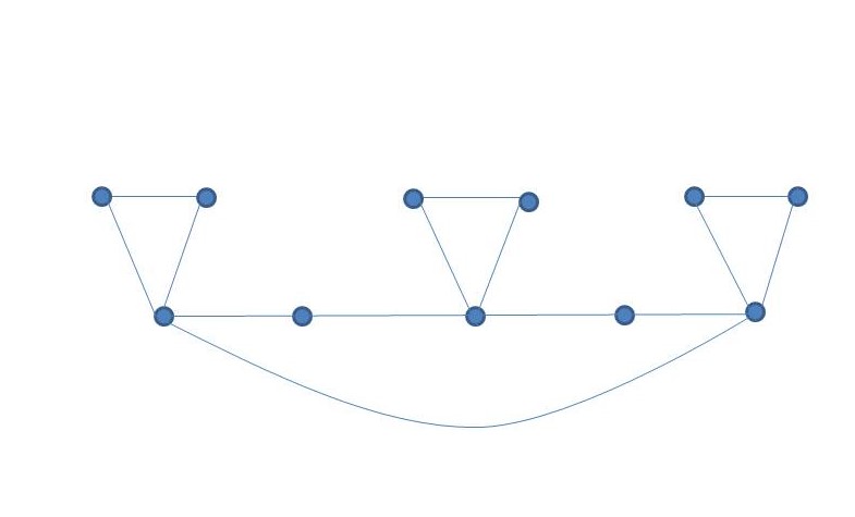
Figure 1: $P_{3}\odot P_{2}$

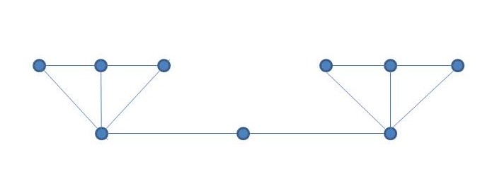
Figure 2: $P_{2}\odot P_{3}$

Figure 3: Figure:1 An example of central vertex corona graphs

Theorem 3.1.

Let $G_{1}$ be an $r_{1}$-regular graph with $n_{1}$ vertices and $m_{1}$ edges and $G_{2}$ be an arbitrary graph with $n_{2}$ vertices. Then the adjacency characteristic polynomial of $G_{1}\odot G_{2}$ is

$$f(A(G_{1}\odot G_{2}),x)= x^{m_{1}-n_{1}}\prod_{j=1}^{n_{2}}(x-\lambda_{j}(G_{2}))^{n_{1}}$$

$$\times\prod_{i=1}^{n_{1}}\left(x^{2}+x-x\chi_{A{(G_{2})}}(x)-r_{1}-xP(\lambda_{i}(G_{1}))+(x-1)\lambda_{i}(G_{1})\right).$$

Proof.

The characteristic polynomial of $G_{1}\odot G_{2}$ is

$$f(A(G_{1}\odot G_{2}),x)= det(xI_{n_{1}+m_{1}+n_{1}n_{2}}-A(G_{1}\odot G_{2}))$$

$$= det\left(\begin{matrix}xI_{n_{1}}-A(\bar{G}_{1})&-I(G_{1})&-I_{n_{1}}\otimes J_{1\times n_{2}}\\ -I(G_{1})^{T}&xI_{m_{1}}&O_{m_{1}\times n_{1}n_{2}}\\ -I_{n_{1}}\otimes J_{1\times n_{2}}^{T}&O_{n_{1}n_{2}\times m_{1}}&I_{n_{1}}\otimes(xI_{n_{2}}-A(G_{2}))\end{matrix}\right).$$

By Lemmas 2.1, 2.2, Definition 2.1 and Corollary 2.6, we have

$$f(A(G_{1}\odot G_{2}),x)= \det(I_{n_{1}}\otimes(xI_{n_{2}}-A(G_{2}))\det S,$$

$$\textnormal{where~{}S}= \begin{pmatrix}xI_{n_{1}}-J_{n_{1}}+I_{n_{1}}+A(G_{1})&{-I(G_{1})}\\ -I(G_{1})^{T}&{xI_{m}}_{1}\\ \end{pmatrix}$$

$$-\begin{pmatrix}-I_{n_{1}}\otimes J_{1\times n_{2}}\\ O_{m_{1}\times n_{1}n_{2}}\end{pmatrix}\left(I_{n_{1}}\otimes(xI_{n_{2}}-A(G_{2}))\right)^{-1}\begin{pmatrix}\-{-I_{n_{1}}\otimes J_{1\times n_{2}}^{T}}&O_{n_{1}n_{2}\times m_{1}}\end{pmatrix}$$

$$= \begin{pmatrix}xI_{n_{1}}-J_{n_{1}}+I_{n_{1}}+A(G_{1})-\chi_{A{(G_{2})}}(x)I_{n_{1}}&-I(G_{1})\\ -I(G_{1})^{T}&xI_{m_{1}}\end{pmatrix}.$$

Therefore,

$$\det S= det\left(\begin{matrix}xI_{n_{1}}-J_{n_{1}}+I_{n_{1}}+A(G_{1})-\chi_{A{(G_{2})}}(x)I_{n_{1}}&-I(G_{1})\\ -I(G_{1})^{T}&{xI_{m}}_{1}\end{matrix}\right)$$

$$= x^{m_{1}}det\left(xI_{n_{1}}-J_{n_{1}}+I_{n_{1}}+A(G_{1})-\chi_{A{(G_{2})}}(x)I_{n_{1}}-\frac{I(G_{1})I(G_{1})^{T}}{x}\right)$$

$$= x^{m_{1}}det\left((x+1-\chi_{A{(G_{2})}}(x))I_{n_{1}}-J_{n_{1}}+A(G_{1})-\frac{I(G_{1})I(G_{1})^{T}}{x}\right)$$

$$= x^{m_{1}}det\left((x+1-\chi_{A{(G_{2})}}(x)-\frac{r_{1}}{x})I_{n_{1}}-J_{n_{1}}+(1-\frac{1}{x})A(G_{1})\right)$$

$$= x^{m_{1}}\prod_{i=1}^{n_{1}}\left(x+1-\chi_{A{(G_{2})}}(x)-\frac{r_{1}}{x}-P(\lambda_{i}(G_{1}))+(1-\frac{1}{x})\lambda_{i}(G_{1})\right).$$

Therefore the adjacency characteristic polynomial of $G_{1}\odot G_{2}$ is

$$f(A(G_{1}\odot G_{2}),x)= \prod_{j=1}^{n_{2}}(x-\lambda_{j}(G_{2}))^{n_{1}}\det S$$

$$= x^{m_{1}-n_{1}}\prod_{j=1}^{n_{2}}(x-\lambda_{j}(G_{2}))^{n_{1}}$$

$$\times\prod_{i=1}^{n_{1}}\left(x^{2}+x-x\chi_{A{(G_{2})}}(x)-r_{1}-xP(\lambda_{i}(G_{1}))+(x-1)\lambda_{i}(G_{1})\right).$$

∎

The following corollary obtained from Theorem 3.1 when $G_{1}$ and $G_{2}$ are both regular graphs.

Corollary 3.2.

Let $G_{i}$ be an $r_{i}$-regular graph with $n_{i}$ vertices and $m_{i}$ edges for ${i=1,2}.$ Then the adjacency characteristic polynomial of $G_{1}\odot G_{2}$ is

$$f(A(G_{1}\odot G_{2}),x)= x^{m_{1}-n_{1}}\left(x^{3}-x^{2}(r_{2}-1-r_{1}+n_{1})-x(r_{2}+n_{2}+2r_{1}+r_{1}r_{2}-n_{1}r_{2})+2r_{1}r_{2}\right)$$

$$\prod_{j=2}^{n_{2}}(x-\lambda_{j}(G_{2}))^{n_{1}}\prod_{i=2}^{n_{1}}\bigg{[}x^{3}-x^{2}(r_{2}-1-\lambda_{i}(G_{1}))-x(r_{2}+n_{2}+r_{1}+$$

$$~{}~{}~{}~{}~{}~{}~{}~{}~{}~{}~{}~{}~{}~{}~{}~{}~{}~{}~{}~{}~{}~{}~{}~{}~{}~{}~{}~{}~{}~{}~{}~{}~{}r_{2}\lambda_{i}(G_{1})+\lambda_{i}(G_{1}))+r_{1}r_{2}+r_{2}\lambda_{i}(G_{1})\bigg{]}.$$

The following corollary describes the complete spectrum of $G_{1}\odot G_{2}$, when $G_{1}$ and $G_{2}$ are both regular graphs.

Corollary 3.3.

Let $G_{i}$ be an $r_{i}$-regular graph with $n_{i}$ vertices and $m_{i}$ edges for ${i=1,2}.$ Then the adjacency spectrum of $G_{1}\odot G_{2}$ consists of

1. $0$, repeated $m_{1}-n_{1}$ times,

2. $\lambda_{j}(G_{2}),$ repeated $n_{1}$ times for $j=2,3,...,n_{2}$,

3. three roots of the equation $x^{3}-x^{2}(r_{2}-1-\lambda_{i}(G_{1}))-x(r_{2}+n_{2}+r_{1}+r_{2}\lambda_{i}(G_{1})+\lambda_{i}(G_{1}))+r_{1}r_{2}+r_{2}\lambda_{i}(G_{1})=0$ for $i=2,...,n_{1},$

4. three roots of the equation $x^{3}-x^{2}(r_{2}-1-r_{1}+n_{1})-x(r_{2}+n_{2}+2r_{1}+r_{1}r_{2}-n_{1}r_{2})+2r_{1}r_{2}=0.$

Example 3.2.

Let $G_{1}=K_{3,3}$ and $G_{2}=K_{2}$. Then the adjacency eigenvalues of $G_{1}$ are 0 (multiplicity $4$) $\pm 3$, eigenvalues of $G_{2}$ are $\pm 1$. Therefore, the adjacency eigenvalues of $G_{1}\odot G_{2}$ are 0 (multiplicity $6$), $-1$ (multiplicity $3$), roots of the equation $x^{3}-6x+3=0$ (each root with multiplicity $4$), roots of the equation $x^{3}-3x^{2}=0$ and roots of the equation $x^{3}-3x^{2}-6x+6=0$ .

Next, we shall consider the adjacency spectrum of $G_{1}\odot G_{2}$ when $G_{1}$ is a regular graph and $G_{2}=K_{p,q}$, $G_{2}$ is non-regular if $p\neq q$.

Corollary 3.4.

Let $G_{1}$ be an $r_{1}$-regular graph with $n_{1}$ vertices and $m_{1}$ edges . Then the adjacency spectrum of $G_{1}\odot K_{p,q}$ consists of

1. $0$, repeated $m_{1}-n_{1}+n_{1}(p+q-2)$ times,

2. four roots of the equation $x^{4}+(1+\lambda_{i}(G_{1}))x^{3}-(pq+p+q+r_{1}+\lambda_{i}(G_{1}))x^{2}+(-3pq-pq\lambda_{i}(G_{1}))x+pq\lambda_{i}(G_{1})+r_{1}pq=0$ for $i=2,...,n_{1},$

3. four roots of the equation $x^{4}+(1+r_{1}-n_{1})x^{3}-(pq+p+q+2r_{1})x^{2}+(-3pq-pqr_{1}+pqn_{1})x+2pqr_{1}=0.$

Corollary 3.2 helps us to construct infinitely many pairs of $A$-cospectral graphs.

Corollary 3.5.

$(a)$ Let $G_{1}$ and $G_{2}$ be $A$-cospectral regular graphs and $H$ is any regular graph. Then $H\odot G_{1}$ and $H\odot G_{2}$ are $A$-cospectral.
$(b)$ Let $G_{1}$ and $G_{2}$ be $A$-cospectral regular graphs and $H$ is any regular graph. Then $G_{1}\odot H$ and $G_{2}\odot H$ are $A$-cospectral.
$(c)$ Let $G_{1}$ and $G_{2}$ be $A$-cospectral regular graphs, $H_{1}$ and $H_{2}$ are another $A$-cospectral regular graphs. Then $G_{1}\odot H_{1}$ and $G_{2}\odot H_{2}$ are $A$-cospectral.

Example 3.3.

Consider the two regular non isomorphic cospectral graphs $G$ and $H$ as in [17]. Graphs $C(G)$ and $C(H)$ as shown in Figure:3. Also, $G\odot K_{2}$ and $H\odot K_{2}$ are non isomorphic. If $G$ and $H$ are regular cospectral graphs, then they have the same regularity with same number of vertices and same number of edges. Since the eigenvalues of $C(G)$ [18] depends on number of vertices, regularity and eigenvalues of $G$. So $C(G)$ and $C(H)$ are $A$-cospectral. By applying Theorem 3.1 on the concerned graphs and comparing their characteristic polynomial we get $G\odot K_{2}$ and $H\odot K_{2}$ are $A$-cospectral graphs.

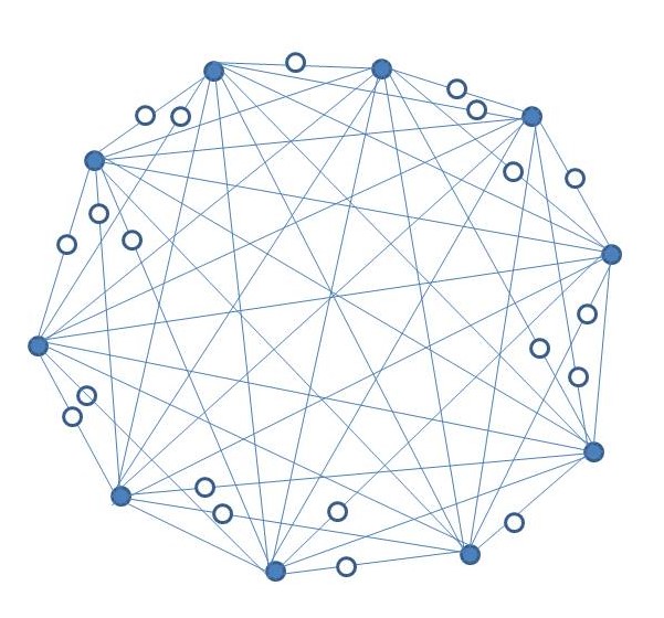
Figure 4: $C(G)$

Figure 5: $C(H)$

Figure 6: Figure:2 Non-regular non isomorphic cospectral graphs

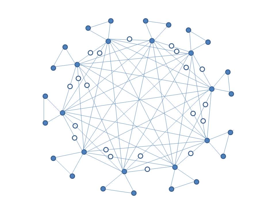
Figure 7: $G\odot K_{2}$

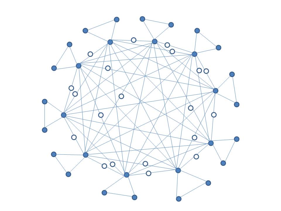
Figure 8: $H\odot K_{2}$

Figure 9: Figure:3 Non-regular non isomorphic $A$-cospectral graphs

Next, we consider the Laplacian characteristic polynomial of $G_{1}\odot G_{2}$ when $G_{1}$ is regular and $G_{2}$ is an arbitrary graph.

Theorem 3.6.

Let $G_{1}$ be an $r_{1}$-regular graph with $n_{1}$ vertices and $m_{1}$ edges and $G_{2}$ be an arbitrary graph with $n_{2}$ vertices. Then the Laplacian characteristic polynomial of $G_{1}\odot G_{2}$ is

$$f(L(G_{1}\odot G_{2}),x)= (x-2)^{m_{1}-n_{1}}\Big{[}x^{3}-x^{2}(n_{2}+r_{1}+3)+x(r_{1}+2n_{1}+2n_{2}+2)\Big{]}$$

$$\times\prod_{j=2}^{n_{2}}\Big{(}x-1-\mu_{j}(G_{2})\Big{)}^{n_{1}}\prod_{i=2}^{n_{1}}\Big{[}x^{3}-x^{2}(n_{1}+n_{2}+3+\lambda_{i}(G_{1})$$

$$+x(n_{2}+3n_{1}+2\lambda_{i}(G_{1})+2-r_{1})-n_{2}-2n_{1}+r_{1}-\lambda_{i}(G_{1}))\Big{]}.$$

Proof.

Let $L(G_{2})$ be the Laplacian matrix of $G_{2}$. Then by a proper labeling of vertices, the Laplacian matrix of $G_{1}\odot G_{2}$ can be written as

$$L(G_{1}\odot G_{2})=\begin{pmatrix}(n_{1}+n_{2}-1)I_{n_{1}}-A(\bar{G_{1}})&-I(G_{1})&-I_{n_{1}}\otimes J_{1\times n_{2}}\\ -I(G_{1})^{T}&2I_{m_{1}}&O_{m_{1}\times n_{1}n_{2}}\\ -I_{n_{1}}\otimes J_{1\times n_{2}}^{T}&O_{n_{1}n_{2}\times m_{1}}&I_{n_{1}}\otimes(I_{n_{2}}+L(G_{2}))\end{pmatrix}.$$

The Laplacian characteristic polynomial of $G_{1}\odot G_{2}$ is

$$f(L(G_{1}\odot G_{2}),x)= det\left(\begin{matrix}(x-n_{1}-n_{2}+1)I_{n_{1}}+A(\bar{G_{1}})&I(G_{1})&I_{n_{1}}\otimes J_{1\times n_{2}}\\ I(G_{1})^{T}&(x-2)I_{m_{1}}&O_{m_{1}\times n_{1}n_{2}}\\ I_{n_{1}}\otimes J_{1\times n_{2}}^{T}&O_{n_{1}n_{2}\times m_{1}}&I_{n_{1}}\otimes((x-1)I_{n_{2}}-L(G_{2}))\end{matrix}\right).$$

By Lemmas 2.1, 2.2, Definition 2.1, equation (2.0.1) and Corollary 2.6, we have

$$f(L(G_{1}\odot G_{2}),x)= det(I_{n_{1}}\otimes((x-1)I_{n_{2}}-L(G_{2})))detS,$$

$$\textnormal{where~{}S}= \begin{pmatrix}(x-n_{1}-n_{2}+1)I_{n_{1}}+A(\bar{G_{1}})&{I(G_{1})}\\ I(G_{1})^{T}&{(x-2)I_{m}}_{1}\\ \end{pmatrix}$$

$$-\begin{pmatrix}\-I_{n_{1}}\otimes J_{1\times n_{2}}\\ O_{{m_{1}}\times{n_{1}n_{2}}}\end{pmatrix}\left(I_{n_{1}}\otimes((x-1)I_{n_{2}}-L(G_{2}))\right)^{-1}\begin{pmatrix}\-I_{n_{1}}\otimes J_{1\times n_{2}}^{T}&O_{n_{1}n_{2}\times m_{1}}\end{pmatrix}$$

$$= \begin{pmatrix}(x-n_{1}-n_{2}+1)I_{n_{1}}+A(\bar{G_{1}})-\chi_{L{(G_{2})}}(x-1)I_{n_{1}}&I(G_{1})\\ I(G_{1})^{T}&{(x-2)I_{m}}_{1}\\ \end{pmatrix}.$$

Therefore,

$$detS= det\left(\begin{matrix}(x-n_{1}-n_{2}+1)I_{n_{1}}+A(\bar{G_{1}})-\chi_{L{(G_{2})}}(x-1)I_{n_{1}}&I(G_{1})\\ I(G_{1})^{T}&{(x-2)I_{m}}_{1}\end{matrix}\right)$$

$$= (x-2)^{m_{1}}det\left((x-n_{1}-n_{2}+1)I_{n_{1}}+A(\bar{G_{1}})-\chi_{L{(G_{2})}}(x-1)I_{n_{1}}-\frac{I(G_{1})I(G_{1})^{T}}{x-2}\right)$$

$$= (x-2)^{m_{1}}det\left((x-n_{1}-n_{2}+1)I_{n_{1}}+J_{n_{1}}-I_{n_{1}}-A(G_{1})-\frac{n_{2}}{x-1}I_{n_{1}}-\frac{A(G_{1})+r_{1}I_{n_{1}}}{x-2}\right)$$

$$= (x-2)^{m_{1}}det\left(\left(x-n_{1}-n_{2}-\frac{n_{2}}{x-1}-\frac{r_{1}}{x-2}\right)I_{n_{1}}+J_{n_{1}}-(1+\frac{1}{x-2})A(G_{1})\right)$$

$$=(x-2)^{m_{1}-n_{1}}\prod_{i=1}^{n_{1}}\left(\left(x-n_{1}-n_{2}-\frac{n_{2}}{x-1}-\frac{r_{1}}{x-2}\right)(x-2)+(x-2)P(\lambda_{i}(G_{1}))-(x-1)\lambda_{i}(G_{1})\right).$$

Note that $\mu_{1}(G_{2})=0$, $P(\lambda_{1}(G_{1}))=n_{1}$ and $P(\lambda_{i}(G_{1}))=0,i=2,...,n_{1}.$
Thus the characteristic polynomial of $L(G_{1}\odot G_{2})$

$$f(L(G_{1}\odot G_{2}),x)= (x-2)^{m_{1}-n_{1}}\Big{[}x^{3}-x^{2}(n_{2}+r_{1}+3)+x(r_{1}+2n_{2}+2)\Big{]}$$

$$\times\prod_{j=2}^{n_{2}}\Big{(}x-1-\mu_{j}(G_{2})\Big{)}^{n_{1}}\prod_{i=2}^{n_{1}}\Big{[}x^{3}-x^{2}(n_{1}+n_{2}+3+\lambda_{i}(G_{1})$$

$$+x(2n_{2}+3n_{1}+2\lambda_{i}(G_{1})+2-r_{1})-2n_{1}+r_{1}-\lambda_{i}(G_{1}))\Big{]}.$$

∎

The following corollary describes the complete Laplacian spectrum of $G_{1}\odot G_{2}$, when $G_{1}$ is a regular graph and $G_{2}$ is an arbitrary graph.

Corollary 3.7.

Let $G_{1}$ be an $r_{1}$-regular graph with $n_{1}$ vertices and $m_{1}$ edges and $G_{2}$ be an arbitrary graph with $n_{2}$ vertices. Then the Laplacian spectrum of $G_{1}\odot G_{2}$ consists of

1. $2$, repeated $m_{1}-n_{1}$ times,

2. $1+\mu_{j}(G_{2})$, repeated $n_{1}$ times for $j=2,3,...,n_{2}$,

3. three roots of the equation $x^{3}-x^{2}(n_{2}+r_{1}+3)+x(r_{1}+2n_{2}+2)=0,$

4. three roots of the equation $x^{3}-x^{2}(n_{1}+n_{2}+3+\lambda_{i}(G_{1}))+x(2n_{2}+3n_{1}+2\lambda_{i}(G_{1})+2-r_{1})-2n_{1}+r_{1}-\lambda_{i}(G_{1}))=0$ for $i=2,3,...,n_{1}.$

Corollary 3.8.

Let $G_{1}$ be an $r_{1}$-regular graph with $n_{1}$ vertices and $m_{1}$ edges and $G_{2}$ be an arbitrary graph with $n_{2}$ vertices . Then the number of spanning trees of $G_{1}\odot G_{2}$ is

$$t(G_{1}\odot G_{2})=\frac{2^{m_{1}-n_{1}}(r_{1}+2n_{2}+2)\prod_{j=2}^{n_{2}}(1+\mu_{j}(G_{2}))^{n_{1}}\prod_{i=2}^{n_{1}}(2n_{1}-r_{1}+\lambda_{i}(G_{1}))}{n_{1}+m_{1}+n_{1}n_{2}}.$$

Corollary 3.9.

Let $G_{1}$ be an $r_{1}$-regular graph with $n_{1}$ vertices and $m_{1}$ edges and $G_{2}$ be an arbitrary graph with $n_{2}$ vertices . Then the Kirchhoff index of $G_{1}\odot G_{2}$ is

$Kf(G_{1}\odot G_{2})=(n_{1}+m_{1}+n_{1}n_{2})\bigg{[}\frac{m_{1}-n_{1}}{2}+\frac{n_{2}+r_{1}+3}{r_{1}+2n_{2}+2}+\displaystyle\sum_{j=2}^{n_{2}}\frac{n_{1}}{1+\mu_{j}(G_{2})}\\ ~{}~{}~{}~{}~{}~{}~{}~{}~{}~{}~{}~{}~{}~{}~{}~{}~{}~{}~{}~{}~{}~{}~{}~{}~{}~{}~{}~{}~{}~{}~{}~{}~{}~{}~{}~{}~{}~{}~{}~{}~{}~{}~{}~{}~{}~{}~{}~{}~{}~{}~{}~{}~{}~{}~{}~{}~{}+\displaystyle\sum_{i=2}^{n_{1}}\frac{2n_{2}+3n_{1}+2\lambda_{i}(G_{1})+2-r_{1}}{2n_{1}-r_{1}+\lambda_{i}(G_{1})}\bigg{]}.$

Corollary 3.7 helps us to construct infinitely many pairs of $L$-cospectral graphs.

Corollary 3.10.

$(a)$ Let $G_{1}$ and $G_{2}$ be $L$-cospectral graphs and $H$ is an arbitarary regular graph. Then $H\odot G_{1}$ and $H\odot G_{2}$ are $L$-cospectral.
$(b)$ Let $G_{1}$ and $G_{2}$ be $L$-cospectral regular graphs and $H$ is an arbitrary graph. Then $G_{1}\odot H$ and $G_{2}\odot H$ are $L$-cospectral.
$(c)$ Let $G_{1}$ and $G_{2}$ be $L$-cospectral regular graphs, $H_{1}$ and $H_{2}$ are another $L$-cospectral regular graphs. Then $G_{1}\odot H_{1}$ and $G_{2}\odot H_{2}$ are $L$-cospectral.

Next, we consider the signless Laplacian characteristic polynomial of $G_{1}\odot G_{2}$ when $G_{1}$ is regular and $G_{2}$ is an arbitrary graph.

Theorem 3.11.

Let $G_{1}$ be an $r_{1}$-regular graph with $n_{1}$ vertices and $m_{1}$ edges and $G_{2}$ be an arbitrary graph with $n_{2}$ vertices. Then the signless Laplacian characteristic polynomial of $G_{1}\odot G_{2}$ is

$$f(Q(G_{1}\odot G_{2}),x) =(x-2)^{m_{1}-n_{1}}\prod_{j=2}^{n_{2}}\Big{(}x-1-\gamma_{j}(G_{2})\Big{)}^{n_{1}}$$

$$\times\prod_{i=1}^{n_{1}}\Bigg{[}\left(x-n_{1}-n_{2}+2-\chi_{Q{(G_{2})}}(x-1)-\frac{r_{1}}{x-2}\right)(x-2)-(x-2)P(\lambda_{i}(G_{1}))+$$

$$~{}~{}~{}~{}~{}~{}~{}~{}~{}~{}~{}~{}~{}~{}~{}~{}~{}~{}~{}~{}~{}~{}~{}~{}~{}~{}~{}~{}~{}~{}~{}~{}~{}~{}~{}~{}~{}~{}~{}~{}~{}~{}~{}~{}~{}~{}~{}~{}~{}~{}~{}~{}~{}~{}~{}~{}~{}~{}~{}~{}~{}~{}(x-3)\lambda_{i}(G_{1})\Bigg{]}$$

Proof.

Let $Q(G_{2})$ be the signless Laplacian matrix of $G_{2}$. Then by a proper labeling of vertices, the signless Laplacian matrix of $G_{1}\odot G_{2}$ can be written as

$$Q(G_{1}\odot G_{2})=\begin{pmatrix}(n_{1}+n_{2}-1)I_{n_{1}}+A(\bar{G_{1}})&I(G_{1})&I_{n_{1}}\otimes J_{1\times n_{2}}\\ I(G_{1})^{T}&2I_{m_{1}}&O_{m_{1}\times n_{1}n_{2}}\\ I_{n_{1}}\otimes J_{1\times n_{2}}^{T}&O_{n_{1}n_{2}\times m_{1}}&I_{n_{1}}\otimes(I_{n_{2}}+Q(G_{2}))\end{pmatrix}.$$

The signless Laplacian characteristic polynomial of $G_{1}\odot G_{2}$ is

$$f(Q(G_{1}\odot G_{2}),x)= det\left(\begin{matrix}(x-n_{1}-n_{2}+1)I_{n_{1}}-A(\bar{G_{1}})&-I(G_{1})&-I_{n_{1}}\otimes J_{1\times n_{2}}\\ -I(G_{1})^{T}&(x-2)I_{m_{1}}&O_{m_{1}\times n_{1}n_{2}}\\ -I_{n_{1}}\otimes J_{1\times n_{2}}^{T}&O_{n_{1}n_{2}\times m_{1}}&I_{n_{1}}\otimes((x-1)I_{n_{2}}-Q(G_{2}))\end{matrix}\right).$$

The rest of the proof is similar to that of Theorem 3.6 and hence we omit details. ∎

Next, we consider the signless Laplacian characteristic polynomial of $G_{1}\odot G_{2}$ when $G_{1}$ and $G_{2}$ are both regular graphs.

Corollary 3.12.

Let $G_{i}$ be an $r_{i}$-regular graph with $n_{i}$ vertices and $m_{i}$ edges for ${i=1,2}.$ Then the signless Laplacian characteristic polynomial of $G_{1}\odot G_{2}$ is

$$f(Q(G_{1}\odot G_{2}),x)$$

$$= (x-2)^{m_{1}-n_{1}}\Big{[}x^{3}-x^{2}(n_{2}+2n_{1}+2r_{2}+1-r_{1})+x(4n_{1}r_{2}+2n_{2}r_{2}+6n_{1}+2n_{2}-4-2r_{2}r_{1}-5r_{1})$$

$$-8n_{1}r_{2}-4n_{2}r_{2}+2r_{1}r_{2}+4r_{1}-4n_{1}+8r_{2}+4+6r_{2}r_{1}\Big{]}\prod_{j=2}^{n_{2}}\Big{(}x-1-\gamma_{j}(G_{2})\Big{)}^{n_{1}}$$

$$\times\prod_{i=2}^{n_{1}}\Big{[}x^{3}-x^{2}(n_{2}+n_{1}+2r_{2}+1-\lambda_{i}(G_{1}))+x(2n_{1}r_{2}+2n_{2}r_{2}+3n_{1}+2n_{2}-r_{1}-4$$

$$-2r_{2}\lambda_{i}(G_{1})-4\lambda_{i}(G_{1}))-4n_{1}r_{2}-4n_{2}r_{2}+2r_{1}r_{2}+3\lambda_{i}(G_{1})+r_{1}+8r_{2}-2n_{1}+6r_{2}\lambda_{i}(G_{1})+4\Big{]}.$$

The following corollary illustrates the signless Laplacian spectrum of $G_{1}\odot G_{2}$, when $G_{1}$ and $G_{2}$ are both regular graphs.

Corollary 3.13.

Let $G_{i}$ be an $r_{i}$-regular graph with $n_{i}$ vertices and $m_{i}$ edges for ${i=1,2}.$ Then the signless Laplacian spectrum of $G_{1}\odot G_{2}$ consists of

1. $2$, repeated $m_{1}-n_{1}$ times,

2. $1+\gamma_{j}(G_{2}),$ repeated $n_{1}$ times for$~{}j=2,3,...,n_{2},$

3. three roots of the equation $x^{3}-x^{2}(n_{2}+2n_{1}+2r_{2}+1-r_{1})+x(4n_{1}r_{2}+2n_{2}r_{2}+6n_{1}+2n_{2}-4-2r_{2}r_{1}-5r_{1})-8n_{1}r_{2}-4n_{2}r_{2}+2r_{1}r_{2}+4r_{1}-4n_{1}+8r_{2}+4+6r_{2}r_{1}=0,$

4. three roots of the equation $x^{3}-x^{2}(n_{2}+n_{1}+2r_{2}+1-\lambda_{i}(G_{1}))+x(2n_{1}r_{2}+2n_{2}r_{2}+3n_{1}+2n_{2}-r_{1}-4-2r_{2}\lambda_{i}(G_{1})-4\lambda_{i}(G_{1}))-4n_{1}r_{2}-4n_{2}r_{2}+2r_{1}r_{2}+3\lambda_{i}(G_{1})+r_{1}+8r_{2}-2n_{1}+6r_{2}\lambda_{i}(G_{1})+4=0$ for $i=2,3,...,n_{1}.$

The following corollary helps us to construct infinitely many pairs of $Q$-cospectral graphs.

Corollary 3.14.

$(a)$ Let $G_{1}$ and $G_{2}$ be $Q$-cospectral regular graphs and $H$ is any regular graph. Then $H\odot G_{1}$ and $H\odot G_{2}$ are $Q$-cospectral.
$(b)$ Let $G_{1}$ and $G_{2}$ be $Q$-cospectral regular graphs and $H$ is any regular graph. Then $G_{1}\odot H$ and $G_{2}\odot H$ are $Q$-cospectral.
$(c)$ Let $G_{1}$ and $G_{2}$ be $Q$-cospectral regular graphs, $H_{1}$ and $H_{2}$ are another $Q$-cospectral regular graphs. Then $G_{1}\odot H_{1}$ and $G_{2}\odot H_{2}$ are $Q$-cospectral.

4 Spectra of central edge corona of graphs

In this section, we define central edge corona of two graphs and calculate their adjacency, Laplacian and signless Laplacian spectrum. Also, we compute the Kirchhoff index and the number of spanning trees of the resulting graphs. Using our results we establish some cospectral graphs.

Definition 4.1.

Let $G_{i}$ be a graph with $n_{i}$ vertices and $m_{i}$ edges for $i=1,2$. The central edge corona $G_{1}\underline{\odot}G_{2}$ of $G_{1}$ and $G_{2}$ is the graph obtained by taking $C(G_{1})$ and $|\tilde{V}(G_{1})|$ copies of $G_{2}$ and joining the $i^{th}$ vertex of $\tilde{V}(G_{1})$ to every vertex in the $i^{th}$ copy of $G_{2}$.
The adjacency matrix of $G_{1}\underline{\odot}G_{2}$ can be written as

$$A(G_{1}\underline{\odot}G_{2})=\begin{pmatrix}A(\overline{G_{1}})&I(G_{1})&O_{n_{1}\times m_{1}n_{2}}\\ I(G_{1})^{T}&O_{m_{1}\times m_{1}}&I_{m_{1}}\otimes J_{1\times n_{2}}\\ O_{m_{1}n_{2}\times n_{1}}&I_{m_{1}}\otimes J_{1\times n_{2}}^{T}&I_{m_{1}}\otimes A(G_{2})\end{pmatrix}.$$

The graph $G_{1}\underline{\odot}G_{2}$ has $n_{1}+m_{1}+m_{1}n_{2}$ vertices and $m_{1}+\frac{n_{1}(n_{1}-1)}{2}+m_{1}m_{2}+m_{1}n_{2}$ edges.

Example 4.1.

Let $G_{1}=P_{3}$ and $G_{2}=P_{2}$. Then the two central edge coronas $G_{1}\underline{\odot}G_{2}$ and $G_{2}\underline{\odot}G_{1}$ are depicted in Figure:4.

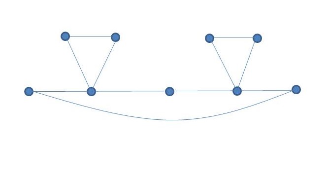
Figure 10: $P_{3}\underline{\odot}P_{2}$

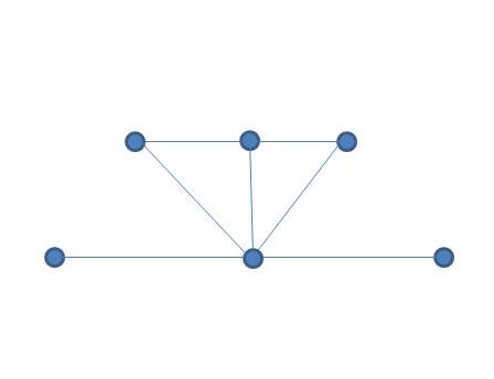
Figure 11: $P_{2}\underline{\odot}P_{3}$

Figure 12: Figure:4 An example of central edge corona graphs

First we consider the adjacency characteristic polynomial of $G_{1}\underline{\odot}G_{2}$.

Theorem 4.1.

Let $G_{1}$ be an $r_{1}$-regular graph with $n_{1}$ vertices and $m_{1}$ edges and $G_{2}$ be an arbitrary graph with $n_{2}$ vertices. Then the adjacency characteristic polynomial of $G_{1}\underline{\odot}G_{2}$ is

$$f(A(G_{1}\underline{\odot}G_{2}),x)= (x-\chi_{A{(G_{2})}}(x))^{m_{1}-n_{1}}\prod_{j=1}^{n_{2}}(x-\lambda_{j}(G_{2}))^{m_{1}}\prod_{i=1}^{n_{1}}\bigg{[}(x+1)(x-\chi_{A(G_{2})}(x))-r_{1}-$$

$$\;\;\;\;\;\;\;\;\;\;\;\;\;\;\;\;\;\;\;\;\;\;P(\lambda_{i}(G_{1}))(x-\chi_{A(G_{2})}(x))+(x-\chi_{A(G_{2})}(x)-1)\lambda_{i}(G_{1})\bigg{]}.$$

Proof.

The characteristic polynomial of $G_{1}\underline{\odot}G_{2}$ is

$$f(A(G_{1}\underline{\odot}G_{2}),x)= det\left(\begin{matrix}xI_{n_{1}}-A(\bar{G}_{1})&-I(G_{1})&O_{n_{1}\times m_{1}n_{2}}\\ -I(G_{1})^{T}&xI_{m_{1}}&-I_{m_{1}}\otimes J_{1\times n_{2}}\\ O_{m_{1}n_{2}\times n_{1}}&-I_{m_{1}}\otimes J_{1\times n_{2}}^{T}&I_{m_{1}}\otimes(xI_{n_{2}}-A(G_{2}))\end{matrix}\right).$$

By Lemmas 2.1, 2.2, Definition 2.1 and Corollary 2.6, we have

$$f(A(G_{1}\underline{\odot}G_{2}),x)= \det(I_{m_{1}}\otimes(xI_{n_{2}}-A(G_{2}))\det S,$$

$$\textnormal{where~{}S}= \begin{pmatrix}xI_{n_{1}}-J_{n_{1}}+I_{n_{1}}+A(G_{1})&{-I(G_{1})}\\ -I(G_{1})^{T}&{xI_{m}}_{1}\\ \end{pmatrix}$$

$$-\begin{pmatrix}O_{n_{1}\times m_{1}n_{2}}\\ -I_{m_{1}}\otimes J_{1\times n_{2}}\end{pmatrix}\left(I_{m_{1}}\otimes xI_{n_{2}}-A(G_{2})\right)^{-1}\begin{pmatrix}\-O_{m_{1}n_{2}\times n_{1}}&-I_{m_{1}}\otimes J_{1\times n_{2}}^{T}\end{pmatrix}$$

$$= \begin{pmatrix}xI_{n_{1}}-J_{n_{1}}+I_{n_{1}}+A(G_{1})&-I(G_{1})\\ -I(G_{1})^{T}&xI_{m_{1}}-\chi_{A{(G_{2})}}(x)I_{m_{1}}\end{pmatrix}.$$

Therefore,

$$det~{}S$$

$$= det\left(\begin{matrix}xI_{n_{1}}-J_{n_{1}}+I_{n_{1}}+A(G_{1})&-I(G_{1})\\ -I(G_{1})^{T}&{xI_{m}}_{1}-\chi_{A{(G_{2})}}(x)I_{m_{1}}\end{matrix}\right)$$

$$= (x-\chi_{A{(G_{2})}}(x))^{m_{1}}det\left(xI_{n_{1}}-J_{n_{1}}+I_{n_{1}}+A(G_{1})-\frac{I(G_{1})I(G_{1})^{T}}{x-\chi_{A{(G_{2})}}(x)}\right)$$

$$= (x-\chi_{A{(G_{2})}}(x))^{m_{1}}det\left((x+1)I_{n_{1}}-J_{n_{1}}+A(G_{1})-\frac{A(G_{1})+r_{1}I_{n_{1}}}{x-\chi_{A{(G_{2})}}(x)}\right)$$

$$= (x-\chi_{A{(G_{2})}}(x))^{m_{1}}det\left((x+1-\frac{r_{1}}{x-\chi_{A{(G_{2})}}(x)})I_{n_{1}}-J_{n_{1}}+(1-\frac{1}{x-\chi_{A{(G_{2})}}(x)})A(G_{1})\right)$$

$$= (x-\chi_{A{(G_{2})}}(x))^{m_{1}}\prod_{i=1}^{n_{1}}\left((x+1-\frac{r_{1}}{x-\chi_{A{(G_{2})}}(x)})-P(\lambda_{i}(G_{1}))+(1-\frac{1}{x-\chi_{A{(G_{2})}}(x)})\lambda_{i}(G_{1})\right)$$

$$= (x-\chi_{A{(G_{2})}}(x))^{m_{1}-n_{1}}\prod_{i=1}^{n_{1}}\bigg{[}(x+1)(x-\chi_{A(G_{2})}(x))-r_{1}-$$

$$\;\;\;\;\;\;\;\;\;\;\;\;\;\;\;\;\;\;\;\;\;\;\;\;\;\;\;\;\;\;\;\;\;P(\lambda_{i}(G_{1}))(x-\chi_{A(G_{2})}(x))+(x-\chi_{A(G_{2})}(x)-1)\lambda_{i}(G_{1})\bigg{]}.$$

Therefore the characteristic polynomial of $G_{1}\underline{\odot}G_{2}$ is

$$f(A(G_{1}\underline{\odot}G_{2}),x)= (x-\chi_{A{(G_{2})}}(x))^{m_{1}-n_{1}}\prod_{j=1}^{n_{2}}(x-\lambda_{j}(G_{2}))^{m_{1}}\prod_{i=1}^{n_{1}}\bigg{[}(x+1)(x-\chi_{A(G_{2})}(x))-r_{1}-$$

$$\;\;\;\;\;\;\;\;\;\;\;\;\;P(\lambda_{i}(G_{1}))(x-\chi_{A(G_{2})}(x))+(x-\chi_{A(G_{2})}(x)-1)\lambda_{i}(G_{1})\bigg{]}.$$

∎

The following corollary gives adjacency characteristic polynomial of $G_{1}\underline{\odot}G_{2}$ when $G_{1}$ and $G_{2}$ are both regular graphs.

Corollary 4.2.

Let $G_{i}$ be an $r_{i}$-regular graph with $n_{i}$ vertices and $m_{i}$ edges for ${i=1,2}.$ Then the adjacency characteristic polynomial of $G_{1}\underline{\odot}G_{2}$ is

$$f(A(G_{1}\underline{\odot}G_{2}),x)= (x^{2}-xr_{2}-n_{2})^{m_{1}-n_{1}}\bigg{[}x^{3}-x^{2}(r_{2}-1+n_{1}-r_{1})+x(-n_{2}-r_{2}+n_{1}r_{2}$$

$$-r_{1}r_{2}-2r_{1})-r_{1}n_{2}+n_{1}n_{2}-n_{2}+2r_{1}r_{2}\bigg{]}\prod_{j=2}^{n_{2}}(x-\lambda_{j}(G_{2}))^{m_{1}}$$

$$\prod_{i=2}^{n_{1}}\bigg{[}x^{3}-x^{2}(r_{2}-\lambda_{i}(G_{1})-1)-x(n_{2}+r_{2}+r_{2}\lambda_{i}(G_{1})+r_{1}+\lambda_{i}(G_{1}))$$

$$~{}~{}~{}~{}~{}~{}~{}~{}~{}~{}~{}~{}~{}~{}~{}~{}~{}~{}~{}~{}~{}~{}~{}~{}~{}~{}~{}~{}~{}~{}~{}~{}~{}~{}~{}~{}~{}~{}~{}-n_{2}\lambda_{i}(G_{1})+r_{2}\lambda_{i}(G_{1})+r_{1}r_{2}-n_{2}\bigg{]}.$$

The following corollary gives the spectrum of $G_{1}\underline{\odot}G_{2}$, when $G_{1}$ and $G_{2}$ are both regular graphs.

Corollary 4.3.

Let $G_{i}$ be an $r_{i}$-regular graph with $n_{i}$ vertices and $m_{i}$ edges for ${i=1,2}.$ Then the adjacency spectrum of $G_{1}\underline{\odot}G_{2}$ consists of

1. $\lambda_{j}(G_{2}),$ repeated $m_{1}$ times for $j=2,3,...,n_{2}$,

2. two roots of the equation $x^{2}-xr_{2}-n_{2}=0,$ each root repeated $m_{1}-n_{1}$ times,

3. three roots of the equation

   $$x^{3}-x^{2}(r_{2}-1+n_{1}-r_{1})+x(-n_{2}-r_{2}+n_{1}r_{2}-r_{1}r_{2}-2r_{1})-r_{1}n_{2}+n_{1}n_{2}-n_{2}+2r_{1}r_{2}=0,$$

4. three roots of the equation $x^{3}-x^{2}(r_{2}-\lambda_{i}(G_{1})-1)-x(n_{2}+r_{2}+r_{2}\lambda_{i}(G_{1})+r_{1}+\lambda_{i}(G_{1}))-n_{2}\lambda_{i}(G_{1})+r_{2}\lambda_{i}(G_{1})+r_{1}r_{2}-n_{2}=0$ for $i=2,3,...,n_{1}.$

Example 4.2.

Let $G_{1}=K_{3,3}$ and $G_{2}=K_{2}$. Then the adjacency eigenvalues of $G_{1}$ are 0 (multiplicity $4$) and $\pm 3$, eigenvalues of $G_{2}$ are $\pm 1$. Therefore, the adjacency eigenvalues of $G_{1}\underline{\odot}G_{2}$ are $-1$ (multiplicity $9$), roots of the equation $x^{2}-x-2=0$ (each root with multiplicity $3$), roots of the equation $x^{3}-3x^{2}-6x+10=0$, roots of the equation $x^{3}-3x^{2}+4=0$ and roots of the equation $x^{3}-6x+1=0$ (each root with multiplicity $4$).

Next, we shall consider the adjacency spectrum of $G_{1}\underline{\odot}G_{2}$ when $G_{1}$ is a regular graph and $G_{2}=K_{p,q}$, $G_{2}$ is non-regular if $p\neq q$.

Corollary 4.4.

Let $G_{1}$ be an $r_{1}$-regular graph with $n_{1}$ vertices and $m_{1}$ edges . Then the adjacency spectrum of $G_{1}\underline{\odot}K_{p,q}$ consists of

1. $0$, repeated $m_{1}(p+q-2)$ times,

2. three roots of the equation $x^{3}-x(pq+p+q)-2pq=0$, each root repeated $m_{1}-n_{1}$ times,

3. four roots of the equation $x^{4}+(1+\lambda_{i})x^{3}-(pq+p+q+r_{1}+\lambda_{i}(G_{1}))x^{2}+(-3pq-p-q-p\lambda_{i}(G_{1})-q\lambda_{i}(G_{1})-pq\lambda_{i}(G_{1}))x-2pq-\lambda_{i}(G_{1})pq+r_{1}pq=0$ for $i=2,...,n_{1},$

4. four roots of the equation_$x^{4}+(1+r_{1}-n_{1})x^{3}-(pq+p+q+2r_{1})x^{2}+(-3pq-p-q+pqn_{1}+pn_{1}+qn_{1}-pqr_{1}-pr_{1}-qr_{1})x-2pq+2pqn_{1}=0.$

Corollary 4.3 helps us to construct infinitely many pairs of $A$-cospectral graphs.

Corollary 4.5.

$(a)$ Let $G_{1}$ and $G_{2}$ be $A$-cospectral regular graphs and $H$ is any regular graph. Then $H\underline{\odot}G_{1}$ and $H\underline{\odot}G_{2}$ are $A$-cospectral.
$(b)$ Let $G_{1}$ and $G_{2}$ be $A$-cospectral regular graphs and $H$ is any regular graph. Then $G_{1}\underline{\odot}H$ and $G_{2}\underline{\odot}H$ are $A$-cospectral.
$(c)$ Let $G_{1}$ and $G_{2}$ be A-cospectral regular graphs, $H_{1}$ and $H_{2}$ are another $A$-cospectral regular graphs. Then $G_{1}\underline{\odot}H_{1}$ and $G_{2}\underline{\odot}H_{2}$ are $A$-cospectral.

Example 4.3.

Consider the two regular non isomorphic cospectral graphs $G$ and $H$ as in [17]. By similar arguments as in Example 3.3, we have $G\underline{\odot}K_{2}$ and $H\underline{\odot}K_{2}$ are $A$-cospectral.

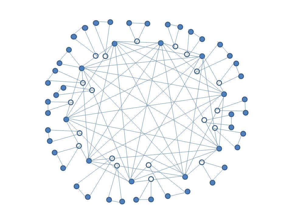
Figure 13: $G\underline{\odot}K_{2}$

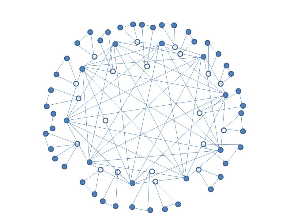
Figure 14: $H\underline{\odot}K_{2}$

Figure 15: Figure:5 Non-regular non isomorphic $A$-cospectral graphs

Next, we discuss the Laplacian characteristic polynomial of $G_{1}\underline{\odot}G_{2}$, when $G_{1}$ is a regular graph and $G_{2}$ is an arbitrary graph.

Theorem 4.6.

Let $G_{1}$ be an $r_{1}$-regular graph with $n_{1}$ vertices and $m_{1}$ edges and $G_{2}$ be an arbitrary graph with $n_{2}$ vertices. Then the Laplacian characteristic polynomial of $G_{1}\underline{\odot}G_{2}$ is

$$f(L(G_{1}\underline{\odot}G_{2}),x)= (x^{2}-x(n_{2}+3)+2)^{m_{1}-n_{1}}\Big{[}x^{3}-x^{2}(n_{2}+r_{1}+3)+x(3r_{1}+n_{2}r_{1}+2)\Big{]}$$

$$\times\prod_{j=2}^{n_{2}}\Big{(}x-1-\mu_{j}(G_{2})\Big{)}^{m_{1}}\prod_{i=2}^{n_{1}}\Big{[}x^{3}-x^{2}(n_{2}+n_{1}+3+\lambda_{i}(G_{1}))$$

$$+x(2+n_{1}n_{2}+3n_{1}-r_{1}+n_{2}\lambda_{i}(G_{1})+4\lambda_{i}(G_{1}))-2n_{1}+r_{1}-\lambda_{i}(G_{1})\Big{]}.$$

Proof.

Let $L(G_{2})$ be the Laplacian matrix of $G_{2}$. Then by a proper labeling of vertices, the Laplacian matrix of $G_{1}\underline{\odot}G_{2}$ can be written as

$$L(G_{1}\underline{\odot}G_{2})=\begin{pmatrix}(n_{1}-1)I_{n_{1}}-A(\bar{G_{1}})&-I(G_{1})&O_{n_{1}\times m_{1}n_{2}}\\ -I(G_{1})^{T}&(n_{2}+2)I_{m_{1}}&-I_{m_{1}}\otimes J_{1\times n_{2}}\\ O_{m_{1}n_{2}\times n_{1}}&-I_{m_{1}}\otimes J_{1\times n_{2}}^{T}&I_{m_{1}}\otimes(I_{n_{2}}+L(G_{2}))\end{pmatrix}.$$

The Laplacian characteristic polynomial of $G_{1}\underline{\odot}G_{2}$ is

$$f(L(G_{1}\underline{\odot}G_{2}),x)= det\left(\begin{matrix}(x-n_{1}+1)I_{n_{1}}+A(\bar{G_{1}})&I(G_{1})&O_{n_{1}\times m_{1}n_{2}}\\ I(G_{1})^{T}&(x-n_{2}-2)I_{m_{1}}&I_{m_{1}}\otimes J_{1\times n_{2}}\\ O_{m_{1}n_{2}\times n_{1}}&I_{m_{1}}\otimes J_{1\times n_{2}}^{T}&I_{m_{1}}\otimes((x-1)I_{n_{2}}-L(G_{2}))\end{matrix}\right).$$

By Lemmas 2.1, 2.2, Corollary 2.6, equation (2.0.1) and Definition 2.1, we have

$$f(L(G_{1}\underline{\odot}G_{2}),x)= det(I_{m_{1}}\otimes((x-1)I_{n_{2}}-L(G_{2})))detS,$$

$$\textnormal{where~{}S}= \begin{pmatrix}(x-n_{1}+1)I_{n_{1}}+A(\bar{G_{1}})&{I(G_{1})}\\ I(G_{1})^{T}&{(x-n_{2}-2)I_{m}}_{1}\\ \end{pmatrix}$$

$$-\begin{pmatrix}O_{n_{1}\times m_{1}n_{2}}\\ I_{m_{1}}\otimes J_{1\times n_{2}}\end{pmatrix}\left(I_{m_{1}}\otimes((x-1)I_{n_{2}}-L(G_{2}))\right)^{-1}\begin{pmatrix}O_{m_{1}n_{2}\times n_{1}}&I_{m_{1}}\otimes J_{1\times n_{2}}^{T}\end{pmatrix}$$

$$= \begin{pmatrix}(x-n_{1}+1)I_{n_{1}}+A(\bar{G_{1}})&I(G_{1})\\ I(G_{1})^{T}&{(x-n_{2}-2)I_{m}}_{1}-\chi_{L{(G_{2})}}(x-1)I_{m_{1}}\\ \end{pmatrix}.$$

Therefore,
det S

$$= det\left(\begin{matrix}(x-n_{1}+1)I_{n_{1}}+A(\bar{G_{1}})&I(G_{1})\\ I(G_{1})^{T}&{(x-n_{2}-2)I_{m}}_{1}-\chi_{L{(G_{2})}}(x-1)I_{m_{1}}\end{matrix}\right)$$

$$= (x-n_{2}-2-\chi_{L{(G_{2})}}(x-1))^{m_{1}}det\left((x-n_{1}+1)I_{n_{1}}+A(\bar{G_{1}})-\frac{I(G_{1})I(G_{1})^{T}}{(x-n_{2}-2-\chi_{L{(G_{2})}}(x-1))}\right)$$

$$= (x-n_{2}-2-\chi_{L{(G_{2})}}(x-1))^{m_{1}}$$

$$\times det\left((x-n_{1}+1)I_{n_{1}}+J_{n_{1}}-I_{n_{1}}-A(G_{1})-\frac{A(G_{1})+r_{1}I_{n_{1}}}{(x-n_{2}-2-\chi_{L{(G_{2})}}(x-1))}\right)$$

$$= (x-n_{2}-2-\chi_{L{(G_{2})}}(x-1))^{m_{1}}$$

$$det\left(\left(x-n_{1}-\frac{r_{1}}{(x-n_{2}-2-\chi_{L{(G_{2})}}(x-1))}\right)I_{n_{1}}+J_{n_{1}}-(1+\frac{1}{(x-n_{2}-2-\chi_{L{(G_{2})}}(x-1))})A(G_{1})\right)$$

$$= (x^{2}-x(n_{2}+3)+2)^{m_{1}-n_{1}}\prod_{i=1}^{n_{1}}\bigg{[}\left((x-n_{1})(x^{2}-x(n_{2}+3)+2)-r_{1}(x-1)\right)+$$

$$\;\;\;\;\;\;\;\;\;\;\;\;\;\;\;\;\;\;\;\;\;\;\;\;\;\;\;\;\;\;\;\;\;\;\;(x^{2}-x(n_{2}+3)+2)P(\lambda_{i}(G_{1}))-(x^{2}-x(n_{2}+3)+3)\lambda_{i}(G_{1})\bigg{]}.$$

Note that $\mu_{1}(G_{2})=0$, $P(\lambda_{1}(G_{1}))=n_{1}$, $P(\lambda_{i}(G_{1}))=0,i=2,...,n_{1}$ .
Thus the characteristic polynomial of $L(G_{1}\underline{\odot}G_{2})$ is

$$f(L(G_{1}\underline{\odot}G_{2}),x)= (x^{2}-x(n_{2}+3)+2)^{m_{1}-n_{1}}\Big{[}x^{3}-x^{2}(n_{2}+r_{1}+3)+x(3r_{1}+n_{2}r_{1}+2)\Big{]}$$

$$\times\prod_{j=2}^{n_{2}}\Big{(}x-1-\mu_{j}(G_{2})\Big{)}^{m_{1}}\prod_{i=2}^{n_{1}}\Big{[}x^{3}-x^{2}(n_{2}+n_{1}+3+\lambda_{i}(G_{1}))$$

$$+x(2+n_{1}n_{2}+3n_{1}-r_{1}+n_{2}\lambda_{i}(G_{1})+4\lambda_{i}(G_{1}))-2n_{1}+r_{1}-\lambda_{i}(G_{1})\Big{]}.$$

∎

The following corollary illustrates the complete Laplacian spectrum of $G_{1}\underline{\odot}G_{2}$, when $G_{1}$ is a regular graph and $G_{2}$ is an arbitrary graph.

Corollary 4.7.

Let $G_{1}$ be an $r_{1}$-regular graph with $n_{1}$ vertices and $m_{1}$ edges and $G_{2}$ be an arbitrary graph with $n_{2}$ vertices. Then the Laplacian spectrum of $G_{1}\underline{\odot}G_{2}$ consists of

1. two roots of the equation $x^{2}-x(n_{2}+3)+2=0$, each root repeated $m_{1}-n_{1}$ times,

2. $1+\mu_{j}(G_{2})$, repeated $m_{1}$ times for $j=2,3,...,n_{2}$,

3. three roots of the equation $x^{3}-x^{2}(n_{2}+r_{1}+3)+x(3r_{1}+n_{2}r_{1}+2)=0,$

4. three roots of the equation $x^{3}-x^{2}(n_{2}+n_{1}+3+\lambda_{i}(G_{1}))+x(2+n_{1}n_{2}+3n_{1}-r_{1}+n_{2}\lambda_{i}(G_{1})+4\lambda_{i}(G_{1}))-2n_{1}+r_{1}-\lambda_{i}(G_{1})=0$ for $i=2,3,...,n_{1}.$

Corollary 4.8.

Let $G_{1}$ be an $r_{1}$-regular graph with $n_{1}$ vertices and $m_{1}$ edges and $G_{2}$ be an arbitrary graph with $n_{2}$ vertices. Then the number of spanning trees of $G_{1}\underline{\odot}G_{2}$ is

$$t(G_{1}\underline{\odot}G_{2})=\frac{2^{m_{1}-n_{1}}(3r_{1}+n_{2}r_{1}+2)\prod_{j=2}^{n_{2}}(1+\mu_{j}(G_{2}))^{m_{1}}\prod_{i=2}^{n_{1}}(2n_{1}-r_{1}+\lambda_{i}(G_{1})}{n_{1}+m_{1}+m_{1}n_{2}}.$$

Corollary 4.9.

Let $G_{1}$ be an $r_{1}$-regular graph with $n_{1}$ vertices and $m_{1}$ edges and $G_{2}$ be an arbitrary graph with $n_{2}$ vertices. Then the Kirchhoff index of $G_{1}\underline{\odot}G_{2}$ is

$Kf(G_{1}\underline{\odot}G_{2})=(n_{1}+m_{1}+m_{1}n_{2})\bigg{[}\frac{(m_{1}-n_{1})(n_{2}+3)}{2}+\frac{n_{2}+r_{1}+3}{3r_{1}+n_{2}r_{1}+2}+\displaystyle\sum_{j=2}^{n_{2}}\frac{m_{1}}{1+\mu_{j}(G_{2})}+\\ ~{}~{}~{}~{}~{}~{}~{}~{}~{}~{}~{}~{}~{}~{}~{}~{}~{}~{}~{}~{}~{}~{}~{}~{}~{}~{}~{}~{}~{}~{}~{}~{}~{}~{}~{}~{}~{}~{}~{}~{}~{}~{}~{}~{}~{}~{}~{}~{}~{}~{}~{}~{}~{}~{}~{}~{}\displaystyle\sum_{i=2}^{n_{1}}\frac{2n_{1}-r_{1}+\lambda_{i}(G_{1})}{2+n_{1}n_{2}+3n_{1}-r_{1}+n_{2}\lambda_{i}(G_{1})+4\lambda_{i}(G_{1})}\bigg{]}.$

The following corollary help us to construct infinitely many pairs of $L$-cospectral graphs.

Corollary 4.10.

$(a)$ Let $G_{1}$ and $G_{2}$ be $L$-cospectral regular graphs and $H$ is an arbitarary graph. Then $H\underline{\odot}G_{1}$ and $H\underline{\odot}G_{2}$ are $L$-cospectral.
$(b)$ Let $G_{1}$ and $G_{2}$ be $L$-cospectral regular graphs and $H$ is an arbitrary graph. Then $G_{1}\underline{\odot}H$ and $G_{2}\underline{\odot}H$ are $L$-cospectral.
$(c)$ Let $G_{1}$ and $G_{2}$ be L-cospectral regular graphs, $H_{1}$ and $H_{2}$ are another $L$-cospectral regular graphs. Then $G_{1}\underline{\odot}H_{1}$ and $G_{2}\underline{\odot}H_{2}$ are $L$-cospectral.

Theorem 4.11.

Let $G_{1}$ be an $r_{1}$-regular graph with $n_{1}$ vertices and $m_{1}$ edges and $G_{2}$ be an arbitrary graph with $n_{2}$ vertices. Then the signless Laplacian characteristic polynomial of $G_{1}\underline{\odot}G_{2}$ is

$$f(Q(G_{1}\underline{\odot}G_{2}),x)= \left(x-n_{2}-2-\chi_{Q{(G_{2})}}(x-1)\right)^{m_{1}-n_{1}}\prod_{j=2}^{n_{2}}\Big{(}x-1-\gamma_{j}(G_{2})\Big{)}^{m_{1}}$$

$$\times\prod_{i=2}^{n_{1}}\Big{[}\Big{(}(x-n_{1}+2)(x-n_{2}-2-\chi_{Q{(G_{2})}}(x-1))-r_{1}\Big{)}I_{n_{1}}$$

$$-(x-n_{2}-2-\chi_{Q{(G_{2})}}(x-1))P(\lambda_{i}(G_{1}))+\Big{(}x-n_{2}-3-\chi_{Q{(G_{2})}}(x-1)\Big{)}\lambda_{i}(G_{1})\Big{]}.$$

Proof.

Let $Q(G_{2})$ be the signless Laplacian matrix of $G_{2}$. Then by a proper labeling of vertices, the Laplacian matrix of $G_{1}\underline{\odot}G_{2}$ can be written as

$$Q(G_{1}\underline{\odot}G_{2})=\begin{pmatrix}(n_{1}-1)I_{n_{1}}+A(\bar{G_{1}})&I(G_{1})&O_{n_{1}\times m_{1}n_{2}}\\ I(G_{1})^{T}&(n_{2}+2)I_{m_{1}}&I_{m_{1}}\otimes J_{1\times n_{2}}\\ O_{m_{1}n_{2}\times n_{1}}&I_{m_{1}}\otimes J_{1\times n_{2}}^{T}&I_{m_{1}}\otimes(I_{n_{2}}+Q(G_{2}))\end{pmatrix}.$$

The signless Laplacian characteristic polynomial of $G_{1}\underline{\odot}G_{2}$ is

$$f(Q(G_{1}\underline{\odot}G_{2}),x)= det\left(\begin{matrix}(x-n_{1}+1)I_{n_{1}}-A(\bar{G_{1}})&-I(G_{1})&O_{n_{1}\times m_{1}n_{2}}\\ -I(G_{1})^{T}&(x-n_{2}-2)I_{m_{1}}&-I_{m_{1}}\otimes J_{1\times n_{2}}\\ O_{m_{1}n_{2}\times n_{1}}&-I_{m_{1}}\otimes J_{1\times n_{2}}^{T}&I_{m_{1}}\otimes((x-1)I_{n_{2}}-Q(G_{2}))\end{matrix}\right).$$

The rest of the proof is similar to that of Theorem 4.6 and hence we omit details. ∎

Next, we consider the signless Laplacian characteristic polynomial of $G_{1}\underline{\odot}G_{2}$ when $G_{1}$ and $G_{2}$ are both regular graphs.

Corollary 4.12.

Let $G_{i}$ be an $r_{i}$-regular graph with $n_{i}$ vertices and $m_{i}$ edges for ${i=1,2}.$ Then the signless Laplacian characteristic polynomial of $G_{1}\underline{\odot}G_{2}$ is

$$f(Q(G_{1}\underline{\odot}G_{2}),x)= (x^{2}-x(2r_{2}+n_{2}+3)+2n_{2}r_{2}+4r_{2}+2)^{m_{1}-n_{1}}\Big{[}x^{3}-x^{2}(n_{2}+2r_{2}+2n_{1}+1-r_{1})+$$

$$x(n_{1}n_{2}+4r_{2}n_{1}+2n_{2}r_{2}+6n_{1}-2n_{2}-4-n_{2}r_{1}-2r_{2}-5r_{1}+n_{1}n_{2})$$

$$-4n_{1}n_{2}r_{2}-8n_{1}r_{2}+4n_{2}r_{2}+8r_{1}r_{2}-4n_{1}+4r_{1}+8r_{2}+4+2n_{2}r_{2}r_{1}-2n_{1}n_{2}\Big{]}$$

$$\times\prod_{j=2}^{n_{2}}\Big{(}x-1-\gamma_{j}(G_{2})\Big{)}^{m_{1}}\prod_{i=2}^{n_{1}}\Big{[}x^{3}-x^{2}(n_{2}+2r_{2}+n_{1}+1-\lambda_{i}(G_{1}))$$

$$+x(n_{1}n_{2}+2r_{2}n_{1}+2n_{2}r_{2}+3n_{1}-2n_{2}-r_{1}-4-n_{2}\lambda_{i}(G_{1})-2r_{2}-4\lambda_{i}(G_{1}))$$

$$-2n_{1}n_{2}r_{2}-4n_{1}r_{2}+4n_{2}r_{2}+2r_{1}r_{2}-2n_{1}+r_{1}+8r_{2}+4+2n_{2}r_{2}\lambda_{i}(G_{1})$$

$$\;\;\;\;\;\;\;\;\;\;\;\;\;\;\;\;\;\;\;\;\;\;\;\;\;\;\;\;\;\;\;\;\;\;\;\;\;\;\;\;\;\;\;\;\;\;\;\;\;\;\;\;\;\;\;\;\;\;\;\;\;\;\;\;\;\;\;\;+6r_{2}\lambda_{i}(G_{1})+3\lambda_{i}(G_{1}))\Big{]}.$$

Next, we consider the signless Laplacian spectra of $G_{1}\underline{\odot}G_{2}$, when $G_{1}$ and $G_{2}$ are both regular graphs.

Corollary 4.13.

Let $G_{i}$ be an $r_{i}$-regular graph with $n_{i}$ vertices and $m_{i}$ edges for ${i=1,2}.$ Then the signless Laplacian spectrum of $G_{1}\underline{\odot}G_{2}$ consists of

1. two roots of the equation $x^{2}-x(2r_{2}+n_{2}+3)+2n_{2}r_{2}+4r_{2}+2=0$, each root repeated $m_{1}-n_{1}$ times,

2. $1+\gamma_{j}(G_{2})$, repeated $m_{1}$ times for $j=2,3,...,n_{2},$

3. three roots of the equation $x^{3}-x^{2}(n_{2}+2r_{2}+2n_{1}+1-r_{1})+x(n_{1}n_{2}+4r_{2}n_{1}+2n_{2}r_{2}+6n_{1}-2n_{2}-4-n_{2}r_{1}-2r_{2}-5r_{1}+n_{1}n_{2})-4n_{1}n_{2}r_{2}-8n_{1}r_{2}+4n_{2}r_{2}+8r_{1}r_{2}-4n_{1}+4r_{1}+8r_{2}+4+2n_{2}r_{2}r_{1}-2n_{1}n_{2}=0,$

4. three roots of the equation $x^{3}-x^{2}(n_{2}+2r_{2}+n_{1}+1-\lambda_{i}(G_{1}))+\\ x(n_{1}n_{2}+2r_{2}n_{1}+2n_{2}r_{2}+3n_{1}-2n_{2}-r_{1}-4-n_{2}\lambda_{i}(G_{1})-2r_{2}-4\lambda_{i}(G_{1}))-2n_{1}n_{2}r_{2}-4n_{1}r_{2}+4n_{2}r_{2}+2r_{1}r_{2}-2n_{1}+r_{1}+8r_{2}+4+2n_{2}r_{2}\lambda_{i}(G_{1})+6r_{2}\lambda_{i}(G_{1})+3\lambda_{i}(G_{1}))=0$ for $i=2,...,n_{1}.$

Corollary 4.12 enables us to construct infinitely many pairs of $Q$-cospectral graphs.

Corollary 4.14.

$(a)$ Let $G_{1}$ and $G_{2}$ be $Q$-cospectral regular graphs and $H$ is any regular graph. Then $H\underline{\odot}G_{1}$ and $H\underline{\odot}G_{2}$ are $Q$-cospectral.
$(b)$ Let $G_{1}$ and $G_{2}$ be $Q$-cospectral regular graphs and $H$ is any regular graph. Then $G_{1}\underline{\odot}H$ and $G_{2}\underline{\odot}H$ are $Q$-cospectral.
$(c)$ Let $G_{1}$ and $G_{2}$ be Q-cospectral regular graphs, $H_{1}$ and $H_{2}$ are another $Q$-cospectral regular graphs. Then $G_{1}\underline{\odot}H_{1}$ and $G_{2}\underline{\odot}H_{2}$ are $Q$-cospectral.

5 Spectra of central edge neighborhood corona of graphs

In this section, we define a new graph operation called central edge neighborhood corona of graphs and determine its adjacency spectrum, Laplacian spectrum, and signless Laplacian spectrum. Also, our results leads us to construct new pairs of cospctral graphs. It is possible to calculate the number of spanning trees and the Kirchhoff index of the resulting graphs.

Operation 5.1.

Let $G_{i}$ be a graph with $n_{i}$ vertices and $m_{i}$ edges for $i=1,2$. Then the central edge neighborhood corona $G_{1}\underline{\boxdot}G_{2}$ of two graphs $G_{1}$ and $G_{2}$ is the graph obtained by taking $C(G_{1})$ and $|\tilde{V}(G_{1})|$ copies of $G_{2}$ and joining the neighbors of the $i^{th}$ vertex of $\tilde{V}(G_{1})$ to every vertex in the $i^{th}$ copy of $G_{2}$.
The adjacency matrix of $G_{1}\underline{\boxdot}G_{2}$ can be written as

$$A(G_{1}\underline{\boxdot}G_{2})=\begin{pmatrix}A(\overline{G_{1}})&I(G_{1})&I(G_{1})\otimes J_{1\times n_{2}}\\ I(G_{1})^{T}&O_{m_{1}\times m_{1}}&O_{m_{1}\times n_{1}n_{2}}\\ I(G_{1})^{T}\otimes J_{1\times n_{2}}^{T}&O_{n_{1}n_{2}\times m_{1}}&I_{m_{1}}\otimes A(G_{2})\end{pmatrix}.$$

The graph $G_{1}\underline{\boxdot}G_{2}$ has $n_{1}+m_{1}+m_{1}n_{2}$ vertices and $m_{1}+\frac{n_{1}(n_{1}-1)}{2}+m_{1}m_{2}+2m_{1}n_{2}$ edges .

Example 5.1.

Let $G_{1}=P_{3}$ and $G_{2}=P_{2}$. Then the two central edge coronas $G_{1}\underline{\boxdot}G_{2}$ and $G_{2}\underline{\boxdot}G_{1}$ are depicted in Figure:6.

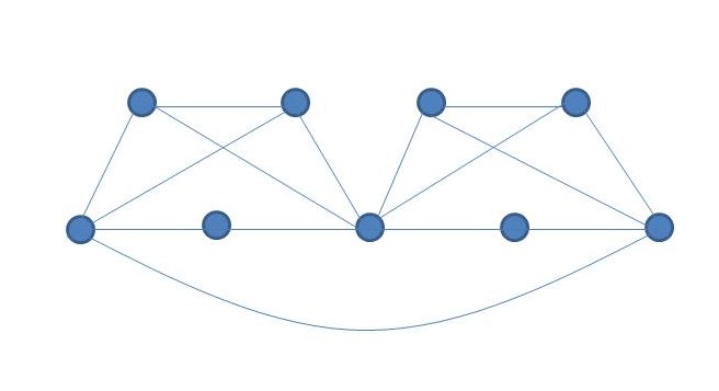
Figure 16: $P_{3}\underline{\boxdot}P_{2}$

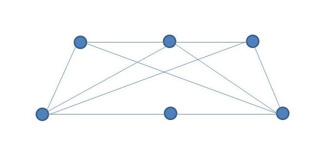
Figure 17: $P_{2}\underline{\boxdot}P_{3}$

Figure 18: Figure:6 An example of central edge neighborhood corona graphs

First we calculate the adjacency characteristic polynomial of $G_{1}\underline{\boxdot}G_{2}$.

Theorem 5.1.

Let $G_{1}$ be an $r_{1}$-regular graph with $n_{1}$ vertices and $m_{1}$ edges and $G_{2}$ be an arbitrary graph with $n_{2}$ vertices. Then the adjacency characteristic polynomial of $G_{1}\underline{\boxdot}G_{2}$ is

$$f(A(G_{1}\underline{\boxdot}G_{2}),x)= x^{m_{1}}\prod_{j=1}^{n_{2}}(x-\lambda_{j}(G_{2}))^{m_{1}}$$

$$\times\prod_{i=1}^{n_{1}}\left((x+1-r_{1}\chi_{A(G_{2})}(x)-\frac{r_{1}}{x})-P(\lambda_{i}(G_{1}))+\left(1-\chi_{A{(G_{2})}}(x)-\frac{1}{x}\right)\lambda_{i}(G_{1})\right).$$

Proof.

The characteristic polynomial of $G_{1}\underline{\boxdot}G_{2}$ is

$$f(A(G_{1}\underline{\boxdot}G_{2}),x)= det\left(\begin{matrix}xI_{n_{1}}-A(\bar{G}_{1})&-I(G_{1})&-I(G_{1})\otimes J_{1\times n_{2}}\\ -I(G_{1})^{T}&xI_{m_{1}}&O_{m_{1}\times n_{1}n_{2}}\\ -I(G_{1})^{T}\otimes J_{1\times n_{2}}^{T}&O_{n_{1}n_{2}\times m_{1}}&I_{m_{1}}\otimes(xI_{n_{2}}-A(G_{2}))\end{matrix}\right).$$

By Lemmas 2.1, 2.2, Definition 2.1 and Corollary 2.6, we have

$$f(A(G_{1}\underline{\boxdot}G_{2}),x)= \det(I_{m_{1}}\otimes(xI_{n_{2}}-A(G_{2}))\det S,$$

$$\textnormal{where~{}S}= \begin{pmatrix}xI_{n_{1}}-J_{n_{1}}+I_{n_{1}}+A(G_{1})&{-I(G_{1})}\\ -I(G_{1})^{T}&{xI_{m}}_{1}\\ \end{pmatrix}$$

$$-\begin{pmatrix}-I(G_{1})\otimes J_{1\times n_{2}}\\ O_{m_{1}\times n_{1}n_{2}}\end{pmatrix}\left(I_{m_{1}}\otimes xI_{n_{2}}-A(G_{2})\right)^{-1}\begin{pmatrix}-{I(G_{1})^{T}\otimes J_{1\times n_{2}}^{T}}&O_{n_{1}n_{2}\times m_{1}}\end{pmatrix}$$

$$= \begin{pmatrix}xI_{n_{1}}-J_{n_{1}}+I_{n_{1}}+A(G_{1})-\chi_{A{(G_{2})}}(x)I(G_{1})I(G_{1})^{T}&-I(G_{1})\\ -I(G_{1})^{T}&xI_{m_{1}}\end{pmatrix}.$$

$$\det S= det\left(\begin{matrix}xI_{n_{1}}-J_{n_{1}}+I_{n_{1}}+A(G_{1})-\chi_{A{(G_{2})}}(x)I(G_{1})I(G_{1})^{T}&-I(G_{1})\\ -I(G_{1})^{T}&{xI_{m}}_{1}\end{matrix}\right)$$

$$= x^{m_{1}}det\left(xI_{n_{1}}-J_{n_{1}}+I_{n_{1}}+A(G_{1})-\chi_{A{(G_{2})}}(x)I(G_{1})I(G_{1})^{T}-\frac{I(G_{1})I(G_{1})^{T}}{x}\right)$$

$$= x^{m_{1}}det\left(xI_{n_{1}}-J_{n_{1}}+I_{n_{1}}+A(G_{1})-\chi_{A{(G_{2})}}(x)(A(G_{1})+r_{1}I_{n_{1}})-\frac{A(G_{1})+r_{1}I_{n_{1}}}{x}\right)$$

$$= x^{m_{1}}det\left(\left(x+1-r_{1}\chi_{A(G_{2})}(x)-\frac{r_{1}}{x}\right)I_{n_{1}}-J_{n_{1}}+\left(1-\chi_{A{(G_{2})}}(x)-\frac{1}{x}\right)A(G_{1})\right).$$

,

Therefore the characteristic polynomial of $G_{1}\underline{\boxdot}G_{2}$ is

$$f(A(G_{1}\underline{\boxdot}G_{2}),x)= x^{m_{1}}\prod_{j=1}^{n_{2}}(x-\lambda_{j}(G_{2}))^{m_{1}}$$

$$\times\prod_{i=1}^{n_{1}}\left(\left(x+1-r_{1}\chi_{A(G_{2})}(x)-\frac{r_{1}}{x}\right)-P(\lambda_{i}(G_{1}))+\left(1-\chi_{A{(G_{2})}}(x)-\frac{1}{x}\right)\lambda_{i}(G_{1})\right).$$

∎

The following corollary gives the adjacency characteristic polynomial of $G_{1}\underline{\boxdot}G_{2}$ when $G_{1}$ and $G_{2}$ are both regular graphs.

Corollary 5.2.

Let $G_{i}$ be an $r_{i}$-regular graph with $n_{i}$ vertices and $m_{i}$ edges for ${i=1,2}.$ Then the adjacency characteristic polynomial of $G_{1}\underline{\boxdot}G_{2}$ is

$$f(A(G_{1}\underline{\boxdot}G_{2}),x)= (x(x-r_{2}))^{m_{1}-n_{1}}\big{[}x^{3}+x^{2}(1-r_{2}+r_{1}-n_{1})-x(2n_{2}r_{1}+2r_{1}+r_{2}+r_{2}r_{1}+$$

$$-n_{1}r_{2})+2r_{1}r_{2}\big{]}\prod_{j=2}^{n_{2}}(x-\lambda_{j}(G_{2}))^{m_{1}}\prod_{i=2}^{n_{1}}\bigg{[}x^{3}+x^{2}(1-r_{2}+\lambda_{i}(G_{1}))$$

$$-x(n_{2}r_{1}+r_{1}+r_{2}+r_{2}\lambda_{i}(G_{1})+n_{2}\lambda_{i}(G_{1})+\lambda_{i}(G_{1}))+r_{1}r_{2}+r_{2}\lambda_{i}(G_{1})\bigg{]}.$$

The following corollary describes the complete spectrum of $G_{1}\underline{\boxdot}G_{2}$, when $G_{1}$ and $G_{2}$ are both regular graphs.

Corollary 5.3.

Let $G_{i}$ be an $r_{i}$-regular graph with $n_{i}$ vertices and $m_{i}$ edges for ${i=1,2}.$ Then the adjacency spectrum of $G_{1}\underline{\boxdot}G_{2}$ consists of

1. $0$, repeated $m_{1}-n_{1}$ times,

2. $r_{2}$, repeated $m_{1}-n_{1}$ times,

3. $\lambda_{j}(G_{2}),$ repeated $m_{1}$ times for $j=2,3,...,n_{2}$,

4. three roots of the equation $x^{3}+x^{2}(1-r_{2}+\lambda_{i}(G_{1}))-x(n_{2}r_{1}+r_{1}+r_{2}+r_{2}\lambda_{i}(G_{1})+n_{2}\lambda_{i}(G_{1})+\lambda_{i}(G_{1}))+r_{1}r_{2}+r_{2}\lambda_{i}(G_{1})=0$ for $i=2,...,n_{1},$

5. three roots of the equation $x^{3}+x^{2}(1-r_{2}+r_{1}-n_{1})-x(2n_{2}r_{1}+2r_{1}+r_{2}+r_{2}r_{1}-n_{1}r_{2})+2r_{1}r_{2}=0.$

Example 5.2.

Let $G_{1}=K_{3,3}$ and $G_{2}=K_{2}$. Then the adjacency eigenvalues of $G_{1}$ are 0 (multiplicity $4$) and $\pm 3$, eigenvalues of $G_{2}$ are $\pm 1$. Therefore, the adjacency eigenvalues of $G_{1}\underline{\boxdot}G_{2}$ are $0$ (multiplicity $3$), $1$ (multiplicity $3$), $-1$ (multiplicity $9$), roots of the equation $x^{2}-x-2=0$ (each root with multiplicity $3$), roots of the equation $x^{3}-3x^{2}-16x+6=0$, roots of the equation $x^{3}-3x^{2}+2x=0$ and roots of the equation $x^{3}-10x+3=0$ (each root with multiplicity $4$).

Next, we shall consider the adjacency spectrum of $G_{1}\underline{\boxdot}G_{2}$ when $G_{1}$ is a regular graph and $G_{2}=K_{p,q}$, $G_{2}$ is non-regular if $p\neq q$.

Corollary 5.4.

Let $G_{1}$ be an $r_{1}$-regular graph with $n_{1}$ vertices and $m_{1}$ edges . Then the adjacency spectrum of $G_{1}\underline{\boxdot}K_{p,q}$ consists of

1. $0$, repeated $m_{1}-n_{1}+m_{1}(p+q-2)$ times,

2. $\pm\sqrt{pq}$, repeated $m_{1}-n_{1}$ times,

3. four roots of the equation $x^{4}+(1+r_{1}-n_{1})x^{3}-(pq+r_{1}p+r_{1}q+2r_{1}+pr_{1}+qr_{1})x^{2}+(-pq-5r_{1}pq+n_{1}pq)x+2r_{1}pq=0$,

4. four roots of the equation $x^{4}+(1+\lambda_{i})x^{3}-(pq+r_{1}p+r_{1}q+r_{1}+(p+q+1)\lambda_{i}(G_{1}))x^{2}+(-pq-2r_{1}pq-3pq\lambda_{i}(G_{1}))x+r_{1}pq+pq\lambda_{i}(G_{1})=0$ for $i=2,...,n_{1}.$

The following corollary enables us to construct infinitely many pairs of $A$-cospectral graphs.

Corollary 5.5.

$(a)$ Let $G_{1}$ and $G_{2}$ be $A$-cospectral regular graphs and $H$ is any regular graph. Then $H\underline{\boxdot}G_{1}$ and $H\underline{\boxdot}G_{2}$ are $A$-cospectral.
$(b)$ Let $G_{1}$ and $G_{2}$ be $A$-cospectral regular graphs and $H$ is any regular graph. Then $G_{1}\underline{\boxdot}H$ and $G_{2}\underline{\boxdot}H$ are $A$-cospectral.
$(c)$ Let $G_{1}$ and $G_{2}$ be $A$-cospectral regular graphs, $H_{1}$ and $H_{2}$ are another $A$-cospectral regular graphs. Then $G_{1}\underline{\boxdot}H_{1}$ and $G_{2}\underline{\boxdot}H_{2}$ are $A$-cospectral.

Next, we consider the Laplacian characteristic polynomial of $G_{1}\underline{\boxdot}G_{2}$.

Theorem 5.6.

Let $G_{1}$ be an $r_{1}$-regular graph with $n_{1}$ vertices and $m_{1}$ edges and $G_{2}$ be an arbitrary graph with $n_{2}$ vertices. Then the Laplacian characteristic polynomial of $G_{1}\underline{\boxdot}G_{2}$ is

$$f(L(G_{1}\underline{\boxdot}G_{2}),x)=(x-2)^{m_{1}-n_{1}}\Big{[}x^{2}-x(n_{2}r_{1}+r_{1}+2)\Big{]}\prod_{j=1}^{n_{2}}\Big{(}x-1-\mu_{j}(G_{2})\Big{)}^{m_{1}}$$

$$\times\prod_{i=2}^{n_{1}}\Big{[}x^{2}-x(2+n_{1}+n_{2}r_{1}+\lambda_{i}(G_{1}))+2n_{1}+n_{2}r_{1}-r_{1}+\lambda_{i}(G_{1})-n_{2}\lambda_{i}(G_{1})\Big{]}.$$

Proof.

Let $L(G_{2})$ be the Laplacian matrix of $G_{2}$. Then by a proper labeling of vertices, the Laplacian matrix of $G_{1}\underline{\boxdot}G_{2}$ can be written as

$$L(G_{1}\underline{\boxdot}G_{2})=\begin{pmatrix}(n_{1}-1+n_{2}r_{1})I_{n_{1}}-A(\bar{G_{1}})&-I(G_{1})&-I(G_{1})\otimes J_{1\times n_{2}}\\ -I(G_{1})^{T}&2I_{m_{1}}&O_{m_{1}\times m_{1}n_{2}}\\ -I(G_{1})^{T}\otimes J_{1\times n_{2}}^{T}&O_{m_{1}n_{2}\times m_{1}}&I_{m_{1}}\otimes(2I_{n_{2}}+L(G_{2}))\end{pmatrix}.$$

The Laplacian characteristic polynomial of $G_{1}\underline{\boxdot}G_{2}$ is

$$f(L(G_{1}\underline{\boxdot}G_{2}),x)= det\left(\begin{matrix}(x-n_{1}+1-n_{2}r_{1})I_{n_{1}}+A(\bar{G_{1}})&I(G_{1})&I(G_{1})\otimes J_{1\times n_{2}}\\ I(G_{1})^{T}&(x-2)I_{m_{1}}&O_{m_{1}\times m_{1}n_{2}}\\ I(G_{1})^{T}\otimes J_{1\times n_{2}}^{T}&O_{m_{1}n_{2}\times m_{1}}&I_{m_{1}}\otimes((x-2)I_{n_{2}}-L(G_{2}))\end{matrix}\right).$$

By Lemmas 2.1, 2.2, Definition 2.1, equation (2.0.1) and Corollary 2.6, we have

$$f(L(G_{1}\underline{\boxdot}G_{2}),x)= det(I_{m_{1}}\otimes((x-2)I_{n_{2}}-L(G_{2})))detS,$$

$$\textnormal{where~{}S}= \begin{pmatrix}(x-n_{1}+1-n_{2}r_{1})I_{n_{1}}+A(\bar{G_{1}})&{I(G_{1})}\\ I(G_{1})^{T}&{(x-2)I_{m}}_{1}\\ \end{pmatrix}$$

$$-\begin{pmatrix}I(G_{1})\otimes J_{1\times n_{2}}\\ O_{m_{1}\times m_{1}n_{2}}\end{pmatrix}\left(I_{m_{1}}\otimes((x-2)I_{n_{2}}-L(G_{2}))\right)^{-1}\begin{pmatrix}I(G_{1})^{T}\otimes J_{1\times n_{2}}^{T}&O_{m_{1}n_{2}\times m_{1}}\end{pmatrix}$$

$$= \begin{pmatrix}(x-n_{1}+1-n_{2}r_{1})I_{n_{1}}+A(\bar{G_{1}})-\chi_{L{(G_{2})}}(x-2)I(G_{1})I(G_{1})^{T}&I(G_{1})\\ I(G_{1})^{T}&{(x-2)I_{m}}_{1}\\ \end{pmatrix}.$$

Therefore, det S

$$= det\left(\begin{matrix}(x-n_{1}+1-n_{2}r_{1})I_{n_{1}}+J_{n_{1}}-I_{n_{1}}-A(G_{1})-\chi_{L{(G_{2})}}(x-2)I(G_{1})I(G_{1})^{T}&I(G_{1})\\ I(G_{1})^{T}&{(x-2)I_{m}}_{1}\end{matrix}\right)$$

$$= (x-2)^{m_{1}}det\left(x-n_{1}-n_{2}r_{1})I_{n_{1}}+J_{n_{1}}-A(G_{1})-\chi_{L{(G_{2})}}(x-2)I(G_{1})I(G_{1})^{T}-\frac{I(G_{1})I(G_{1})^{T}}{x-2}\right)$$

$$= (x-2)^{m_{1}}det\left(x-n_{1}-n_{2}r_{1})I_{n_{1}}+J_{n_{1}}-A(G_{1})-\chi_{L{(G_{2})}}(x-2)(A(G_{1})+r_{1}I_{n_{1}})-\frac{A(G_{1})+r_{1}I_{n_{1}}}{x-2}\right)$$

$$= (x-2)^{m_{1}}det\left(\left(x-n_{1}-n_{2}r_{1}-r_{1}\chi_{L(G_{2})}(x-2)-\frac{r_{1}}{x-2}\right)I_{n_{1}}+J_{n_{1}}-\left(1+\chi_{L(G_{2})}(x-2)+\frac{1}{x-2}\right)A(G_{1})\right).$$

Note that $\mu_{1}(G_{2})=0$, $P(\lambda_{1}(G_{1}))=n_{1}$,$P(\lambda_{i}(G_{1}))=0,i=2,...,n_{1}$ .
Thus the characteristic polynomial of $L(G_{1}\underline{\boxdot}G_{2})$ is

$$f(L(G_{1}\underline{\boxdot}G_{2}),x)=(x-2)^{m_{1}-n_{1}}\Big{[}x^{2}-x(n_{2}r_{1}+r_{1}+2)\Big{]}\prod_{j=1}^{n_{2}}\Big{(}x-1-\mu_{j}(G_{2})\Big{)}^{m_{1}}$$

$$\times\prod_{i=2}^{n_{1}}\Big{[}x^{2}-x(2+n_{1}+n_{2}r_{1}+\lambda_{i}(G_{1}))+2n_{1}+n_{2}r_{1}-r_{1}+\lambda_{i}(G_{1})-n_{2}\lambda_{i}(G_{1})\Big{]}.$$

∎

The following corollary describes the complete Laplacian spectrum of $G_{1}\underline{\boxdot}G_{2}$, when $G_{1}$ is a regular graph and $G_{2}$ is an arbitrary graph.

Corollary 5.7.

Let $G_{1}$ be an $r_{1}$-regular graph with $n_{1}$ vertices and $m_{1}$ edges and $G_{2}$ be an arbitrary graph with $n_{2}$ vertices. Then the Laplacian spectrum of $G_{1}\underline{\boxdot}G_{2}$ consists of

1. $2$, repeated $m_{1}-n_{1}$ times,

2. $1+\mu_{j}(G_{2})$, repeated $m_{1}$ times for $j=1,2,3,...,n_{2},$

3. two roots of the equation $x^{2}-x(n_{2}r_{1}+r_{1}+2)=0,$

4. two roots of the equation $x^{2}-x(2+n_{1}+n_{2}r_{1}+\lambda_{i}(G_{1}))+2n_{1}+n_{2}r_{1}-r_{1}+(1-n_{2})\lambda_{i}(G_{1})=0$ for $i=2,3,...,n_{1}.$

Corollary 5.8.

Let $G_{1}$ be an $r_{1}$-regular graph with $n_{1}$ vertices and $m_{1}$ edges and $G_{2}$ be an arbitrary graph with $n_{2}$ vertices. Then the number of spanning trees of $G_{1}\underline{\boxdot}G_{2}$ is

$$t(G_{1}\underline{\boxdot}G_{2})=\frac{2^{m_{1}-n_{1}}(n_{2}r_{1}+r_{1}+2)\prod_{j=1}^{n_{2}}(1+\mu_{j}(G_{2}))^{m_{1}}\prod_{i=2}^{n_{1}}\left[2n_{1}+n_{2}r_{1}-r_{1}+\lambda_{i}(G_{1})-n_{2}\lambda_{i}(G_{1})\right]}{n_{1}+m_{1}+m_{1}n_{2}}.$$

Corollary 5.9.

Let $G_{1}$ be an $r_{1}$-regular graph with $n_{1}$ vertices and $m_{1}$ edges and $G_{2}$ be an arbitrary graph with $n_{2}$ vertices. Then the Kirchhoff index of $G_{1}\underline{\boxdot}G_{2}$ is

$Kf(G_{1}\underline{\boxdot}G_{2})=(n_{1}+m_{1}+m_{1}n_{2})\bigg{[}\frac{m_{1}-n_{1}}{2}+\frac{1}{n_{2}r_{1}+r_{1}+2}+\displaystyle\sum_{j=2}^{n_{2}}\frac{m_{1}}{1+\mu_{j}(G_{2})}+\\ ~{}~{}~{}~{}~{}~{}~{}~{}~{}~{}~{}~{}~{}~{}~{}~{}~{}~{}~{}~{}~{}~{}~{}~{}~{}~{}~{}~{}~{}~{}~{}~{}~{}~{}~{}~{}~{}~{}~{}~{}~{}~{}~{}~{}~{}~{}~{}~{}~{}~{}~{}~{}~{}~{}~{}~{}~{}~{}~{}~{}~{}~{}~{}~{}~{}~{}~{}~{}~{}~{}~{}~{}``\displaystyle\sum_{i=2}^{n_{1}}\frac{2+n_{1}+n_{2}r_{1}+\lambda_{i}(G_{1})}{2n_{1}+n_{2}r_{1}-r_{1}+\lambda_{i}(G_{1})-n_{2}\lambda_{i}(G_{1})}\bigg{]}.$

The following corollary helps us to construct infinitely many pairs of $L$-cospectral graphs.

Corollary 5.10.

$(a)$ Let $G_{1}$ and $G_{2}$ be $L$-cospectral regular graphs and $H$ is an arbitarary graph. Then $H\underline{\boxdot}G_{1}$ and $H\underline{\boxdot}G_{2}$ are $L$-cospectral.
$(b)$ Let $G_{1}$ and $G_{2}$ be $L$-cospectral regular graphs and $H$ is an arbitrary graph. Then $G_{1}\underline{\boxdot}H$ and $G_{2}\underline{\boxdot}H$ are $L$-cospectral.
$(c)$ Let $G_{1}$ and $G_{2}$ be $L$-cospectral regular graphs, $H_{1}$ and $H_{2}$ are another $L$-cospectral regular graphs. Then $G_{1}\underline{\boxdot}H_{1}$ and $G_{2}\underline{\boxdot}H_{2}$ are $L$-cospectral.

Next we consider the signless Laplacian characteristic polynomial of $G_{1}\odot G_{2}$ when $G_{1}$ is regular and $G_{2}$ is an arbitrary graph.

Theorem 5.11.

Let $G_{1}$ be an $r_{1}$-regular graph with $n_{1}$ vertices and $m_{1}$ edges and $G_{2}$ be an arbitrary graph with $n_{2}$ vertices. Then the signless Laplacian characteristic polynomial of $G_{1}\underline{\boxdot}G_{2}$ is

$$f(Q(G_{1}\underline{\boxdot}G_{2}),x) =(x-2)^{m_{1}-n_{1}}\prod_{j=2}^{n_{2}}\Big{(}x-1-\gamma_{j}(G_{2})\Big{)}^{m_{1}}$$

$$\times\prod_{i=1}^{n_{1}}\Bigg{[}\left(x-n_{1}+2-n_{2}r_{1}-r_{1}\chi_{Q(G_{2})}(x-2)-\frac{r_{1}}{x-2}\right)-P(\lambda_{i}(G_{1}))+$$

$$~{}~{}~{}~{}~{}~{}~{}~{}~{}~{}~{}~{}~{}~{}~{}~{}~{}~{}~{}~{}~{}~{}~{}~{}~{}~{}~{}~{}~{}~{}~{}~{}~{}~{}(1-\chi_{Q(G_{2})}(x-2)-\frac{1}{x-2})\lambda_{i}(G_{1})\Bigg{]}$$

Proof.

Let $Q(G_{2})$ be the signless Laplacian matrix of $G_{2}$. Then by a proper labeling of vertices, the Laplacian matrix of $G_{1}\underline{\boxdot}G_{2}$ can be written as

$$Q(G_{1}\underline{\boxdot}G_{2})=\begin{pmatrix}(n_{1}-1+r_{1}n_{2})I_{n_{1}}+A(\bar{G_{1}})&I(G_{1})&I(G_{1})\otimes J_{1\times n_{2}}\\ I(G_{1})^{T}&2I_{m_{1}}&O_{m_{1}\times m_{1}n_{2}}\\ I(G_{1})^{T}\otimes J_{1\times n_{2}}^{T}&O_{m_{1}n_{2}\times m_{1}}&I_{m_{1}}\otimes(2I_{n_{2}}+Q(G_{2}))\end{pmatrix}.$$

The signless Laplacian characteristic polynomial of $G_{1}\underline{\boxdot}G_{2}$ is

$$f(Q(G_{1}\underline{\boxdot}G_{2}),x)= det\left(\begin{matrix}(x-n_{1}+1-r_{1}n_{2})I_{n_{1}}-A(\bar{G_{1}})&-I(G_{1})&-I(G_{1})\otimes J_{1\times n_{2}}\\ -I(G_{1})^{T}&(x-2)I_{m_{1}}&O_{n_{1}\times m_{1}n_{2}}\\ -I(G_{1})^{T}\otimes J_{1\times n_{2}}^{T}&O_{m_{1}n_{2}\times n_{1}}&I_{m_{1}}\otimes((x-2)I_{n_{2}}-Q(G_{2}))\end{matrix}\right).$$

The rest of the proof is similar to that of Theorem 5.6 and hence we omit details. ∎

Next we consider the signless Laplacian characteristic polynomial of $G_{1}\odot G_{2}$ when $G_{1}$ and $G_{2}$ are both regular graphs.

Corollary 5.12.

Let $G_{i}$ be an $r_{i}$-regular graph with $n_{i}$ vertices and $m_{i}$ edges for ${i=1,2}.$ Then the signless Laplacian characteristic polynomial of $G_{1}\underline{\boxdot}G_{2}$ is

$$f(Q(G_{1}\underline{\boxdot}G_{2}),x)$$

$$= (x-2)^{m_{1}-n_{1}}\Big{[}x^{3}-x^{2}(n_{2}r_{1}+2r_{2}+2-r_{1}+2n_{1})+x(2n_{2}r_{1}r_{2}-n_{2}r_{1}-2r_{2}r_{1}+4n_{1}r_{2}+3n_{2}r_{1}-6r_{1}+$$

$$8n_{1}-4)-4n_{2}r_{1}r_{2}+6r_{2}r_{1}-8n_{1}r_{2}+2r_{1}r_{2}+6r_{1}-8n_{1}+2r_{1}+8r_{2}+8\Big{]}$$

$$\times\prod_{j=2}^{n_{2}}\Big{(}x-1-\gamma_{j}(G_{2})\Big{)}^{m_{1}}\prod_{i=2}^{n_{1}}\Big{[}x^{3}-x^{2}(n_{2}r_{1}+2r_{2}+n_{1}+2-\lambda_{i}(G_{1}))+x(2n_{2}r_{1}r_{2}-n_{2}\lambda_{i}(G_{1})$$

$$-2r_{2}\lambda_{i}(G_{1})+2n_{1}r_{2}+3n_{2}r_{1}-5\lambda_{i}(G_{1})+4n_{1}-r_{1}-4)+(-4n_{2}r_{1}r_{2}-2n_{2}\lambda_{i}(G_{1})+6r_{2}\lambda_{i}(G_{1}))$$

$$\;\;\;\;\;\;\;\;\;\;\;\;\;\;\;\;\;\;\;\;\;\;\;\;\;\;\;\;\;\;\;\;\;\;\;\;\;\;\;\;\;\;\;\;\;\;\;\;\;-4n_{1}r_{2}-2n_{2}r_{1}+2r_{1}r_{2}+6\lambda_{i}(G_{1})-4n_{1}+2r_{1}+8r_{2}+8\Big{]}.$$

The signless Laplacian spectrum of $G_{1}\underline{\boxdot}G_{2}$ is obtained from the following corollary.

Corollary 5.13.

Let $G_{i}$ be an $r_{i}$-regular graph with $n_{i}$ vertices and $m_{i}$ edges for ${i=1,2}.$ Then the signless Laplacian spectrum of $G_{1}\underline{\boxdot}G_{2}$ consists of

1. $2$, repeated $m_{1}-n_{1}$ times,

2. $1+\gamma_{j}(G_{2})$, repeated $m_{1}$ times for $j=2,3,...,n_{2},$

3. three roots of the equation $x^{3}-x^{2}(n_{2}r_{1}+2r_{2}+2-r_{1}+2n_{1})+x(2n_{2}r_{1}r_{2}-n_{2}r_{1}-2r_{2}r_{1}+4n_{1}r_{2}+3n_{2}r_{1}-6r_{1}+8n_{1}-4)-4n_{2}r_{1}r_{2}+6r_{2}r_{1}-8n_{1}r_{2}+2r_{1}r_{2}+6r_{1}-8n_{1}+2r_{1}+8r_{2}+8=0,$

4. three roots of the equation $x^{3}-x^{2}(n_{2}r_{1}+2r_{2}+n_{1}+2-\lambda_{i}(G_{1}))+x(2n_{2}r_{1}r_{2}-n_{2}\lambda_{i}(G_{1})-2r_{2}\lambda_{i}(G_{1})+2n_{1}r_{2}+3n_{2}r_{1}-5\lambda_{i}(G_{1})+4n_{1}-r_{1}-4)+(-4n_{2}r_{1}r_{2}-2n_{2}\lambda_{i}(G_{1})+6r_{2}\lambda_{i}(G_{1}))-4n_{1}r_{2}-2n_{2}r_{1}+2r_{1}r_{2}+6\lambda_{i}(G_{1})-4n_{1}+2r_{1}+8r_{2}+8=0$ for $i=2,...,n_{1}.$

The following corollary helps us to construct infinitely many pairs of $Q$-cospectral graphs.

Corollary 5.14.

$(a)$ Let $G_{1}$ and $G_{2}$ be $Q$-cospectral regular graphs and $H$ is any regular graph. Then $H\underline{\boxdot}G_{1}$ and $H\underline{\boxdot}G_{2}$ are $Q$-cospectral.
$(b)$ Let $G_{1}$ and $G_{2}$ be $Q$-cospectral regular graphs and $H$ is any regular graph. Then $G_{1}\underline{\boxdot}H$ and $G_{2}\underline{\boxdot}H$ are $Q$-cospectral.
$(c)$ Let $G_{1}$ and $G_{2}$ be $Q$-cospectral regular graphs, $H_{1}$ and $H_{2}$ are another $Q$-cospectral regular graphs. Then $G_{1}\underline{\boxdot}H_{1}$ and $G_{2}\underline{\boxdot}H_{2}$ are $Q$-cospectral.

6 Conclusion

In this paper, we determine the different types of spectra of central vertex corona, central edge corona, and central edge neighborhood corona of regular graphs. As an application of these results we construct infinitely many pairs of $A$-cospectral, $L$-cospectral and $Q$-cospectral graphs. Further, we compute the number of spanning trees and the Kirchhoff index of these graphs.

References

- [1] Chris Godsil and Gordon F Royle. Algebraic graph theory, volume 207. Springer Science & Business Media, 2001.
- [2] Douglas J Klein and Milan Randić. Resistance distance. Journal of mathematical chemistry, 12(1):81–95, 1993.
- [3] Haiyan Chen and Fuji Zhang. Resistance distance and the normalized Laplacian spectrum. Discrete applied mathematics, 155(5):654–661, 2007.
- [4] Ivan Gutman and Bojan Mohar. The quasi-Wiener and the Kirchhoff indices coincide. Journal of chemical information and computer sciences, 36(5):982–985, 1996.
- [5] H-Y Zhu, Douglas J Klein, and István Lukovits. Extensions of the Wiener number. Journal of chemical information and computer sciences, 36(3):420–428, 1996.
- [6] Frank Harary and Roberto Frucht. On the corona of two graphs. Aequationes mathematicae, 4:322–325, 1970.
- [7] Xiaogang Liu and Pengli Lu. Spectra of subdivision-vertex and subdivision-edge neighbourhood coronae. Linear algebra and its applications, 438(8):3547–3559, 2013.
- [8] Jie Lan and Bo Zhou. Spectra of graph operations based on R-graph. Linear and Multilinear Algebra, 63(7):1401–1422, 2015.
- [9] Ch Adiga, BR Rakshith, and KN Subba Krishna. Spectra of some new graph operations and some new classes of integral graphs. Iranian Journal of Mathematical Sciences and Informatics, 13(1):51–65, 2018.
- [10] Chandrashekar Adiga and BR Rakshith. Spectra of graph operations based on corona and neighborhood corona of the graphs and . Journal of the international mathematical virtual institute, 5:55–69, 2015.
- [11] Roger A Horn and Charles R Johnson. Topics in matrix analysis. Cambridge university press. Cambridge, UK, 1991.
- [12] Dragoš M Cvetković, Michael Doob, and Horst Sachs. Spectra of graphs, theory and applications, volume 10. Academic Press, New York, 1980.
- [13] Arpita Das and Pratima Panigrahi. Spectra of R-vertex join and R-edge join of two graphs. Discussiones Mathematicae-General Algebra and Applications, 38(1):19–31, 2018.
- [14] Cam McLeman and Erin McNicholas. Spectra of coronae. Linear algebra and its applications, 435(5):998–1007, 2011.
- [15] Xiaogang Liu and Zuhe Zhang. Spectra of subdivision-vertex join and subdivision-edge join of two graphs. Bulletin of the Malaysian Mathematical Sciences Society, 42(1):15–31, 2019.
- [16] J Vernold Vivin, MM Akbar Ali, and K Thilagavathi. On harmonious coloring of central graphs. Advances and applications in discrete mathematics, 2(1):17–33, 2008.
- [17] Edwin R Van Dam and Willem H Haemers. Which graphs are determined by their spectrum? Linear Algebra and its applications, 373:241–272, 2003.
- [18] TK Jahfar and AV Chithra. Central vertex join and central edge join of two graphs. AIMS Mathematics, 5(6):7214–7233, 2020.