^†^† ^* Authors contributed equally, ¹ Mila, Polytechnique Montréal, ² Deepmind, ³ Mila, Polytechnique Montréal, ⁴ Element AI, ⁵ Google AI, ⁶Max Planck Institute for Intelligent Systems, ^$\dagger$ CIFAR Senior Fellow Corresponding authors: rosemary.nan.ke@gmail.com

Systematic Evaluation of Causal Discovery in Visual Model Based Reinforcement Learning

Nan Rosemary Ke ^*,1,2 Aniket Didolkar^*,3 Sarthak Mittal ³ Anirudh Goyal ³
Guillaume Lajoie ³ Stefan Bauer ⁶ Danilo Rezende ²
Yoshua Bengio ^{3, $\dagger$} Michael Mozer ⁵ Christopher Pal ^1,4

Abstract

Inducing causal relationships from observations is a classic problem in machine learning. Most work in causality starts from the premise that the causal variables themselves are observed. However, for AI agents such as robots trying to make sense of their environment, the only observables are low-level variables like pixels in images. To generalize well, an agent must induce high-level variables, particularly those which are causal or are affected by causal variables. A central goal for AI and causality is thus the joint discovery of abstract representations and causal structure. However, we note that existing environments for studying causal induction are poorly suited for this objective because they have complicated task-specific causal graphs which are impossible to manipulate parametrically (e.g., number of nodes, sparsity, causal chain length, etc.). In this work, our goal is to facilitate research in learning representations of high-level variables as well as causal structures among them. In order to systematically probe the ability of methods to identify these variables and structures, we design a suite of benchmarking RL environments. We evaluate various representation learning algorithms from the literature and find that explicitly incorporating structure and modularity in models can help causal induction in model-based reinforcement learning.

1 Introduction

Deep learning methods have made immense progress on many reinforcement learning (RL) tasks in recent years. However, the performance of these methods still pales in comparison to human abilities in many cases. Contemporary deep reinforcement learning models have a ways to go to achieve robust generalization (Nichol et al., 2018), efficient planning over flexible timescales (Silver and Ciosek, 2012), and long-term credit assignment (Osband et al., 2019). Model-based methods in RL (MBRL) can potentially mitigate this issue (Schrittwieser et al., 2019). These methods observe sequences of state-action pairs, and from these observations are able to learn a self-supervised model of the environment. With a well-trained world model, these algorithms can then simulate the environment and look ahead to future events to establish better value estimates, without requiring expensive interactions with the environment (Sutton, 1991). Model-based methods can thus be far more sample-efficient than their model-free counterparts when multiple objectives are to be achieved in the same environment. However, for model-based approaches to be successful, the learned models must capture relevant mechanisms that guide the world, i.e., they must discover the right causal variables and structure. Indeed, models sensitive to causality have been shown to be robust and easily transferable (Bengio et al., 2019; Ke et al., 2019). As a result, there has been a recent surge of interest in learning causal models for deep reinforcement learning (de Haan et al., 2019; Dasgupta et al., 2019; Nair et al., 2019; Goyal et al., 2019; Goyal and Bengio, 2020; Rezende et al., 2020; Wang et al., 2021; Schölkopf et al., 2021). Yet, many challenges remain, and a systematic framework to modulate environment causality structure and evaluate models’ capacity to capture it is currently lacking, which motivates this paper.

What limits the use of causal modeling approaches in many AI tasks and realistic RL settings is that most of the current causal learning literature presumes abstract domain representations in which the cause and effect variables are explicit and given (Pearl, 2009). Methods are needed to automate the inference and identification of such causal variables (i.e. causal induction) from low-level state representations (like images). Although one solution is manual labeling, it is often impractical and in some cases impossible to manually label all the causal variables. In some domains, the causal structure may not be known. Further, critical causal variables may change from one task to another, or from one environment to another. And in unknown environments, one ideally aims for an RL agent that could induce the causal structure of the environment from observations and interventions.

In this work, we seek to evaluate various model-based approaches parameterized to exploit structure of environments purposfully designed to modulate causal relations. We find that modular network architectures appear particularly well suited for causal learning. Our conjecture is that causality can provide a useful source of inductive bias to improve the learning of world models.

Shortcomings of current RL development environments, and a path forward. Most existing RL environments are not a good fit for investigating causal induction in MBRL, as they have a single fixed causal graph, lack proper evaluation and have entangled aspects of causal learning. For instance, many tasks have complicated causal structures as well as unobserved confounders. These issues make it difficult to measure progress for causal learning. As we look towards the next great challenges for RL and AI, there is a need to better understand the implications of varying different aspects of the underlying causal graph for various learning procedures.

Hence, to systematically study various aspects of causal induction (i.e., learning the right causal graph from pixel data), we propose a new suite of environments as a platform for investigating inductive biases, causal representations, and learning algorithms. The goal is to disentangle distinct aspects of causal learning by allowing the user to choose and modulate various properties of the ground truth causal graph, such as the structure and size of the graph, the sparsity of the graph and whether variables are observed or not (see Figure 1 (a)-(d)). We also provide evaluation criteria for measuring causal induction in MBRL that we argue help measure progress and facilitate further research in these directions. We believe that the availability of standard experiments and a platform that can easily be extended to test different aspects of causal modeling will play a significant role in speeding up progress in MBRL.

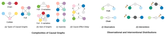
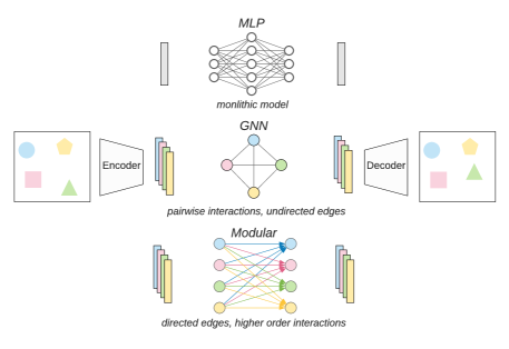
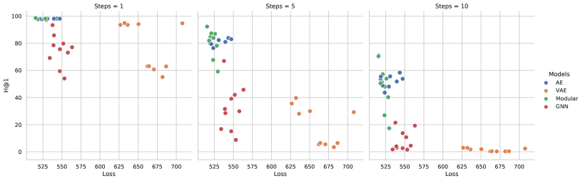
Refer to caption — Figure 1: (a)-(d): Different aspects contributing to the complexity of causal graphs. (i), (ii): Difference between observational and interventional data. In RL setting, actions are interventions in the environment. The hammer denotes an intervention. Intervention on a variable not only affects its direct children, but also all reachable variables. Variables impacted by the intervention have a darker shade.

Insights and causally sufficient inductive biases. Using our platform, we investigate the impact of explicit structure and modularity for causal induction in MBRL. We evaluated two typical of monolithic models (autoencoders and variational autoencoders) and two typical models with explicit structure: graph neural networks (GNNs) and modular models (shown in Figure 5). Graph neural networks (GNNs) have a factorized representation of variables and can model undirected relationships between variables. Modular models also have a factorized representation of variables, along with directed edges between variables which can model directed relationship such as $A$ causing $B$ , but not the other way around. We investigated the performance of such structured approaches on learning from causal graphs with varying complexity, such as the size of the graph, the sparsity of the graph and the length of cause-effect chains (Figure 1 (a) - (d)).

The proposed environment gives novel insights in a number of settings. Especially, we found that even our naive implementation of modular networks can scale significantly better compared to other models (including graph neural networks). This suggests that explicit structure and modularity such as factorized representations and directed edges between variables help with causal induction in MBRL. We also found that graph neural networks, such as the ones from Kipf et al. (2019) are good at modeling pairwise interactions and significantly outperform monolithic models under this setting. However, they have difficulty modeling complex causal graphs with long cause-effect chains, such as the chain graph (demonstration of chain graphs are found in Figure 1 (i)). Another finding is that evaluation metrics such as likelihood and ranking loss do not always correspond to the performance of these models in downstream RL tasks.

2 Environments for causal induction in model-based RL

Causal models are frequently described using graphs in which the edges represent causal relationships. In these structural causal models, the existence of a directed edge from $A$ to $B$ indicates that intervening on $A$ directly impacts $B$ , and the absence of an edge indicates no direct interventional impact (see Appendix B for formal definitions).

In parallel, world models in MBRL describe the underlying data generating process of the environment by modeling the next state given the current state-action pair, where the actions are interventions in the environment. Hence, learning world models in MBRL can be seen as a causal induction problem. Below, we first outline how a collection of simple causal structures can capture real-world MBRL cases, and we propose a set of elemental environments to express them for training. Second, we describe precise ways to evaluate models in these environments.

2.1 Mini-environments: explicit cases for causal modulation in RL

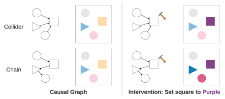
The ease with which an agent learns a task greatly depends on the structure of the environment’s underlying causal graph. For example, it might be easier to learn causal relationships in a collider graph ( see Figure 1(a)) where all interactions are pairwise, meaning that an intervention on one variable $X_{i}$ impacts no more than one other variable $X_{j}$ , hence the cause-effect chain has a length of at most 1. However, causal graphs such as full graphs (see Figure 1 (a)) can have more complex causal interactions, where intervening on one variable impacts can impact up to $n-1$ variables for graphs of size $n$ (see Figure 1). Therefore, one important aspect of understanding a model’s performance on causal induction in MBRL is to analyze how well the model performs on causal graphs of varying complexity.

Impotant factors that contribute to the complexity of discovering the causal graph are the structure, size, sparsity of edges and length of cause-effect chains of the causal graph (Figure 1). Presence of unobserved variables also adds to the complexity. The size of the graph increases complexity because the number of possible graphs grows super-exponentially with the size of the graph (Eaton and Murphy, 2007; Peters et al., 2016; Ke et al., 2019). The sparsity of graphs also impacts the difficulty of learning, as observed in (Ke et al., 2019). Given graphs of the same size, denser graphs are often more challenging to learn. Futhermore, the length of the cause-effect chains can also impact learning. We have observed in our experiments, that graphs with shorter cause-effect lengths such as colliders (Figure 1 (a)) can be easier to model as compared to chain graphs with longer cause-effect chains. Finally, unobserved variables which commonly exist in the real-world can greatly impact learning, especially if they are confounding causes (shared causes of observed variables).

Taking these factors into account, we designed two suites of (toy) environments: the physics environment and the chemistry environment, which we discuss in more detail in the following section. They are designed with a focus on the underlying causal graph and thus have a minimalist design that is easy to visualize.

2.1.1 Physics environment: Weighted-block pushing

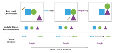
The physics environment simulates very simple physics in the world. It consists of blocks of different, unique weights. The rule for interaction between blocks is that heavier objects can push lighter ones. Interventions ammount to move a particular block, and the consequence depends on whether the block next to it (if present) is heavier or lighter. For an accurate world model, inferring the weights becomes essential. Additionally, one can allow the weight of the objects to be either observed through the intensity of the color, or unobserved, leading to two environment settings described below. The underlying causal graph is an acyclic tournament, shown in Figure 3. For more details about the setup, please refer to Appendix F.

Fully observed setting. In the fully observed setting, all objects are given a particular color and the weight of each block is represented by the intensity of the color. Once the agent learns this underlying causal structure, it does not have to perform interventions on new objects in order to infer they will interact with the others.

Unobserved setting. In this setting, the weight of each object is not directly observable by its color. The agent thus needs to interact with the object in order to understand the order of weights associated with the blocks. In this case, the weight of objects needs to be inferred through interventions. We consider two sub-divisions of this setting - FixedUnobserved where there is a fixed assignment between the shapes of the objects and their weights and Unobserved where there is no fixed assignment between the shape and the weight, hence making it a more challenging environment. We refer the reader to Section F.2 for details.

2.1.2 Chemistry environment

The chemistry environment enables more complexity in the causal structure of the world by allowing arbitrary causal graphs. This is depicted by simple chemical reactions, where the state of an element can cause changes to another variable’s state. The environment consists of a number of objects whose positions are kept fixed and thus, uniquely identifiable.

The interactions between different objects take place according to the underlying causal graph which can either be a randomly generated DAG, or specified by the user. An interaction consists of changing the color (state) of a variable. At this point, the color of all variables affected by this variable (according to the causal graph) can change. Interventions change a block’s color unconditionally, thus cutting the graph edge linking it with its parents in the graph. All transitions are probabilistic and defined by conditional probability tables (CPTs). A visualization of the environment can be found in Figure 4.

This environment allows for a complete and thorough testing of causal models as there are various degrees of complexities which can be easily tuned such as: (1) Complexity of the graph: We can test any model on many different graphs thus ensuring that a models performance is not only limited to a few select graphs. (2) Stochasticity: By tuning the skewness of the probability distribution of each object we can test how good is a given model in modelling data uncertainty. In addition to this we can also tune the number of object or the number of colors to test whether the model generalizes to larger graphs and more colors. A causally correct model should be able to infer the causal relationships between observed objects, as well as their respective color distribution and its dependence on a causal parent’s distribution.

2.2 Evaluating causal models

In much of the existing literature, evaluation of learned causal models is based on the structural difference between the learned graph and the ground-truth graph (Peters et al., 2016; Zheng et al., 2018). However, this may not be applicable for most deep RL algorithms, as they do not necessarily learn an explicit causal structure (Dasgupta et al., 2019; Ke et al., 2020). Even if a structure is learned, it may not be unique as several variable permutations can be equivalent, introducing an additional evaluation burden.

Another possibility is to exhaustively evaluate models on all possible intervention predictions and all environment states, a process that quickly becomes intractable even for small environments.

We therefore propose a few evaluation methods that can be used as a surrogate metrics to measure the model’s performance on recovering the correct causal structure.

Predicting Intervention Outcomes. While it may not be feasible to predict all intervention outcomes in an RL environment, we propose that evaluating predictions on a subset of interventions provides an informative evaluation. Here, the test data is collected from the same environment used in training, ensuring a single underlying causal graph. Test data is generated from new episodes that are unseen during training. All interventions (actions) in the test episodes are randomly sampled and we evaluate the model’s performance on this test set.

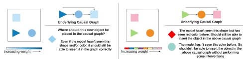
Zero Shot Transfer. Here, we test the model’s ability to generalize to unseen test environments, where the environment does not have exactly the same causal graph as training, but training and test causal graphs share some similarity.

For example, in the observed Physics environment, a model that has learned the underlying causal relationship between color intensity and weight would be able to generalize to new variables with a novel color intensity.

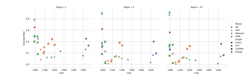
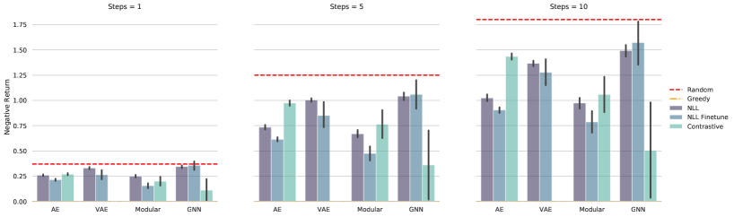
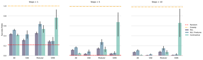
Downstream RL Tasks. Downstream RL tasks that require a good understanding of the underlying causal graph of the environment are also good metrics for measuring the model’s performance. For example, in the physics environment, we can provide the model with a target configuration in the form of some specific arrangement of blocks on a grid and the model needs to perform actions in the environment to reach the target configuration. Models that capture causal relationships between objects should achieve the target configuration more easily (as it is can predict intervention outcomes). For more details about this setup, please refer to Appendix D.

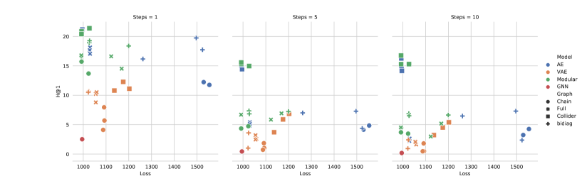
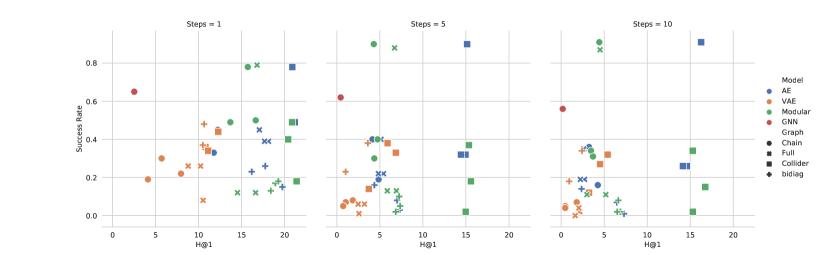
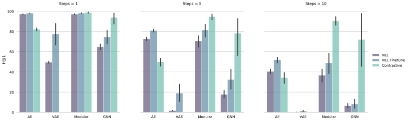
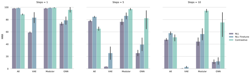
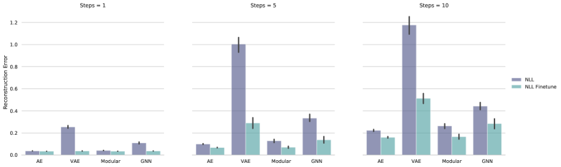
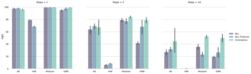
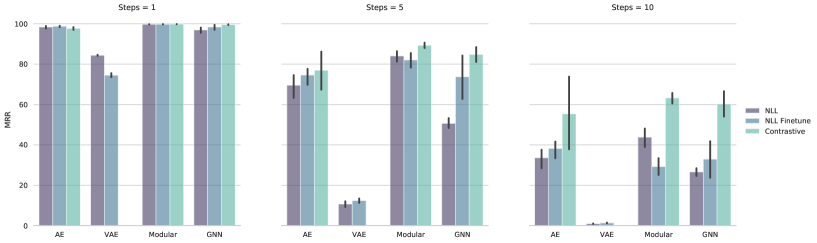
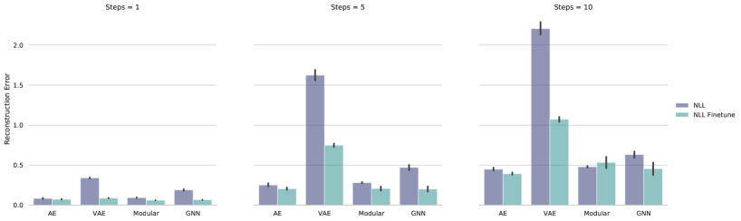
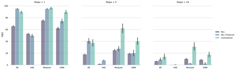
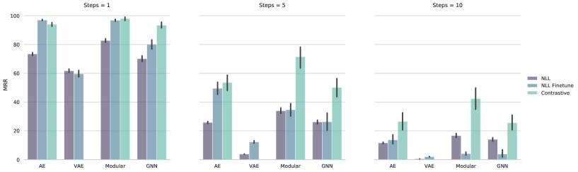
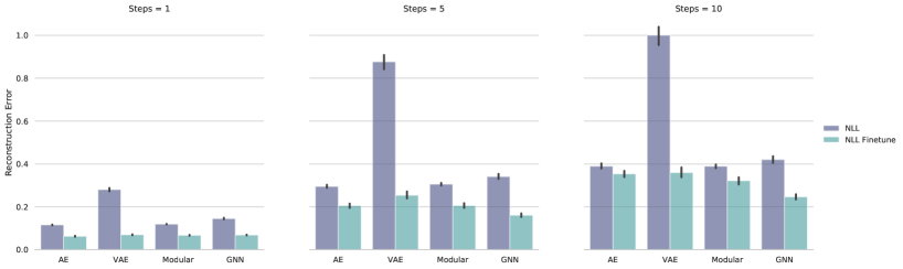
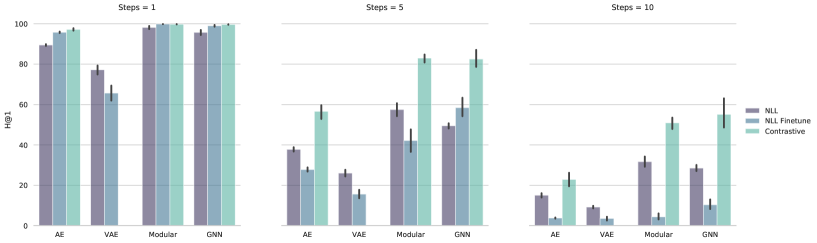
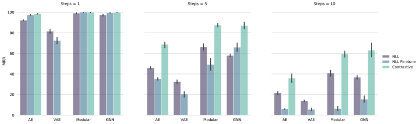
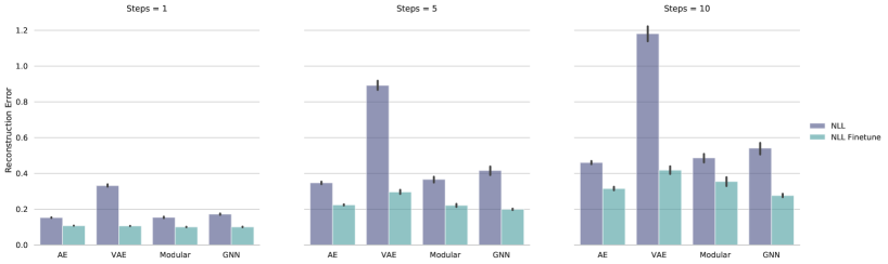
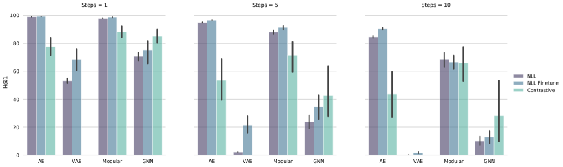
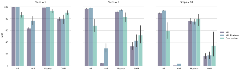
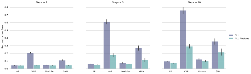
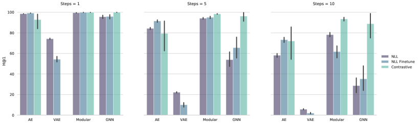
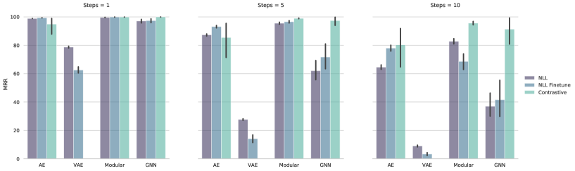
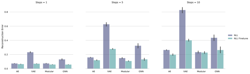
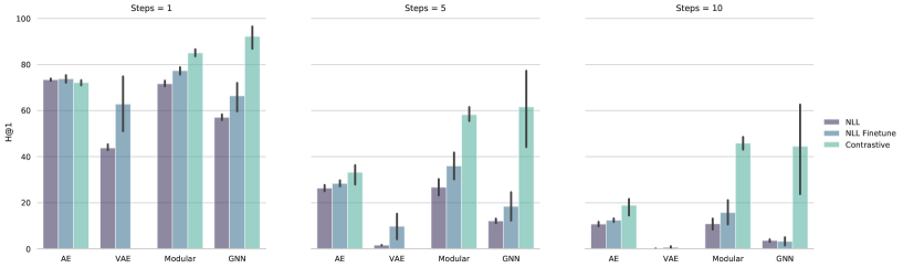
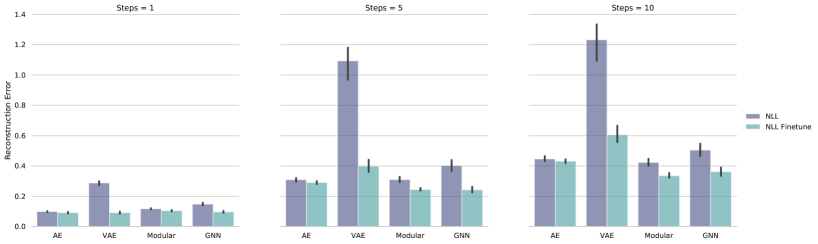
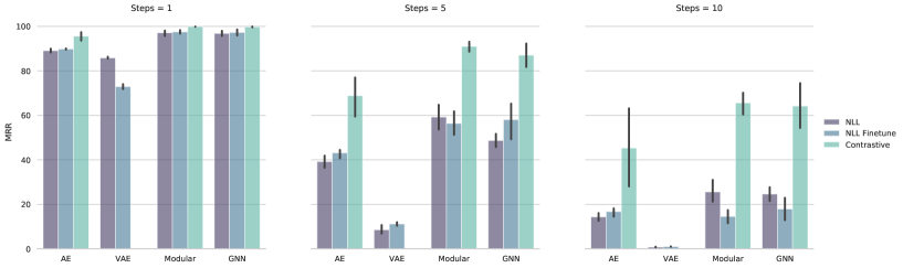
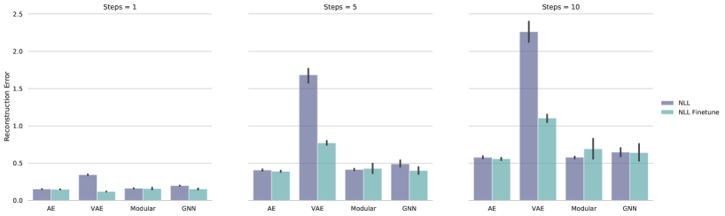
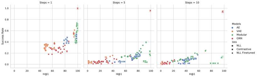
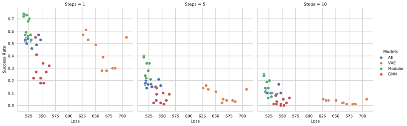
Metrics. We also evaluate the learned models on ranking metrics in the latent space as well as reconstruction-based metrics in the observation space (Kipf et al., 2019). In particular we measure and report Hits at Rank 1 (H@1), Mean Reciprocal Rank (MRR) and Reconstruction loss for evaluation in standard as well as transfer testing settings. We report these metrics for 1, 5 and 10 steps of prediction in the latent space (refer Appendix C).

3 Models

A large variety of neural network models have been proposed as world models in MBRL. These models can roughly be divided into two categories: monolithic models and models that have structure and modularity. Monolithic models typically have no explicit structure (other than layers). Some typical monolithic models are Autoencoders and Variational Autoencoders (Kingma and Welling, 2013; Rezende et al., 2014). Conversely, structured models have explicit architecture built into (or learned by) the model. Examples of such models are ones based on graph neural networks (Battaglia et al., 2016; Van Steenkiste et al., 2018; Kipf et al., 2019; Veerapaneni et al., 2020) and modular models (Ke et al., 2020; Goyal et al., 2019; Mittal et al., 2020; Goyal et al., 2020). We picked some commonly used models from these categories and evaluated their performance to understand their ability for causal induction in MBRL.

To disentangle the architectural biases and effects of different training methodologies, we trained all the models on both likelihood based and contrastive losses, respectively. All models share three common components: encoder, decoder and transition model. We follow a similar training procedure as in Ha and Schmidhuber (2018); Kipf et al. (2019). Details of the architectures as well as the training protocols and losses can be found in Appendix E.

3.1 Monolithic Models

We evaluate causal induction on two commonly used monolithic models: multilayered autoencoders and variational autoencoders. We follow a similar setup as in Ha and Schmidhuber (2018). These models do not have strong inductive biases other than the number of layers used.

3.2 Modular and Structured Models

Several forms of structure can be included in neural networks, including modularity, factorized variables, and directed rules.

Taking the three factors into account, we consider two types of structured models in our paper, graph neural networks (GNN) and so called modular networks. Graph neural networks (GNN) (Gilmer et al., 2017; Tacchetti et al., 2018; Battaglia et al., 2018; Kipf et al., 2019) is a widely adopted relational model that have a factorized representation of variables and models pairwise interactions between objects while being permutation invariant. In particular, we consider the C-SWM model (Kipf et al., 2019), which is a state-of-art GNN used for modeling object interactions. Similar to most GNNs, the C-SWM model learns factorized representations of different objects but for modelling dynamics it considers all possible pairwise interactions, and hence the transition model is monolithic (i.e., not a modular transition model).

Modular networks on the other hand are composed of an initial encoder that factorizes inputs (images), and then a modular transition model (MTM) - $M$ . This internal model is tasked to create separate factored representations for each objects in the environment, while taking into account all other objects’ representations. This model also learns interactions between objects. The rules learned here are directed rules.

4 Experiments

Our experiments seak to answer the following questions: (a) Does explicit structure and modularity help for causal induction in MBRL? If so, then what type of structures provide good inductive bias for causal induction in MBRL? (b) How do different objective functions (likelihood or contrastive) impact learning? (c) How do different models scale to complex causal graphs? (d) Do prediction metrics (likelihood and ranking metrics) correspond to better downstream RL performance? (e) What are good evaluation criteria for causal induction in MBRL?

We report the performance of our models on both the Physics and the Chemistry environments, and refer the readers to Appendix E for implementation details.. All models are trained using the procedure described in Section E.2 and are evaluated based on ranking and likelihood metrics on $1,5$ and $10$ step predictions. For the Chemistry environment, we evaluate the models on causal graphs with varying complexity, namely - chain, collider and full graphs. These graphs vary in the sparsity of edges and the length of cause-effect chains. For the Physics environment, we evaluate the model in the fully observed setting as well as the unobserved setting.

4.1 Explicit structure and causal induction

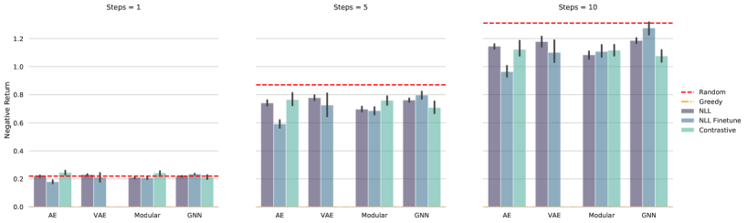
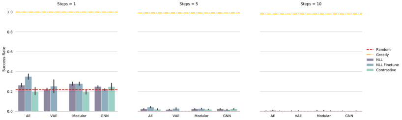
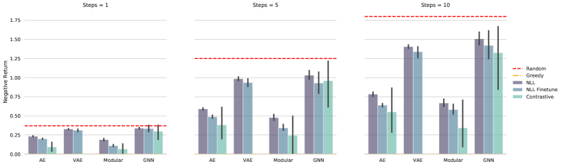
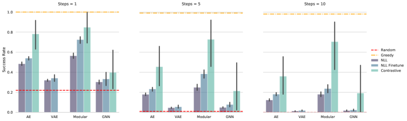
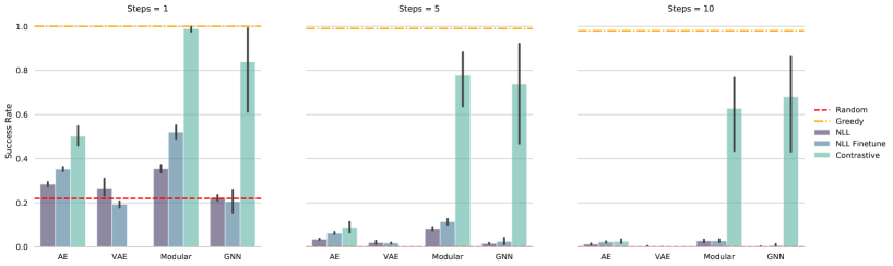
We found that for both the Physics and the Chemistry environments, models with explicit structure outperform monolithic models on both prediction metrics and downstream RL performances. In particular, models with explicit structure (GNNs and modular models) scale better to graphs of larger size and longer cause-effect chains.

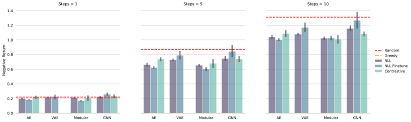
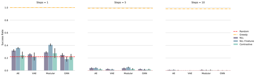
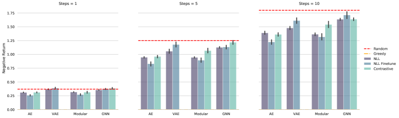
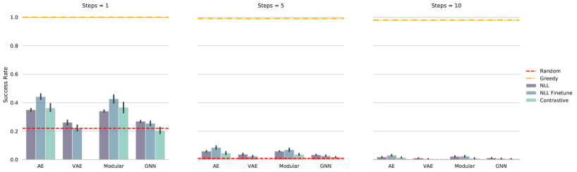
The Physics environment has a complex underlying causal graph (full graph: refer Figure 1 (a)). We found that GNNs performed well in this environment with 3 variables. They achieved good prediction metrics (Figure 7) and high RL performance (Figure 13) even at longer timescales. However, their performance drops significantly on environments with 5 objects both in terms of prediction metrics (Figure 8) and RL performance (Figure 14). We also see in Figures 8 and 14 that modular models scale much better compared to all other models, suggesting that they hold an advantage for larger causal graphs. Further, modular models and GNNs when evaluated on zero shot settings outperform monolithic models by a significant margin (Figures 19 and 20 and Tables 15 and 16).

For the chemistry environment, we find that modular models outperform all other models for almost all causal graphs in terms of both prediction metrics (Figure 23) and RL performance (Figure 25). This is especially true on more complex causal graphs, such as chain and full graphs which have long cause-effect chains. This suggests that modular models scales better to more complex causal graphs.

Overall, these results suggest that structure, and in particular modularity, help causal induction in MBRL when scaling up to larger and more complex causal graphs. The performance comparisons on modular networks and C-SWM (Kipf et al., 2019) suggest that both factorized representation of variables and directed edges between variables can help for causal induction in MBRL.

4.2 Complexity of the Underlying Causal Graph

There are several ways to vary complexity in a causal graph: size of the graph, sparsity of edges and length of cause-effect chain (Figure 1). Increasing the size of the graph significantly impacts all models’ performances. We evaluate models on the Physics environments with 3 objects (Figure 7) and 5 objects (Figure 8) and find that increasing the number of objects from 3 to 5 has a significant impact on performance. Modular models achieve over $90$ on ranking metrics over 10-step prediction for 3 objects while for 5 objects, they achieve only $50$ (almost half the performance on 3 objects). A similar pattern is found in almost all models. Another factor impacting complexity of the graph is the length of cause-effect chain.We see that collider graphs are the easiest to learn, with modular models and autoencoders significantly outpeforming all other models (Figure 23). This is because the collider graph has short pair-wise interactions, i.e, intervention on any node in a collider graph can impact at most one other node. Chain and full graphs are significantly more challenging because of longer cause-effect chains. For a chain or a full graph of $n$ nodes, an intervention on the $k^{th}$ node can impact all the subsequent $(n-k)$ nodes. Modeling interventions on chain and full graphs require modeling more than pairwise relationships, hence, making it much more challenging. We find that modular models slightly outperform all other models on these graphs.

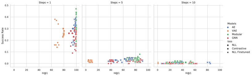
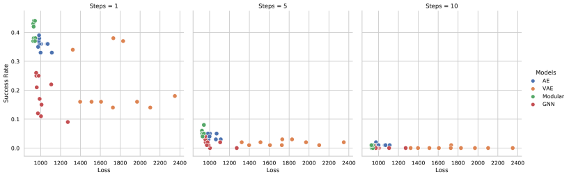
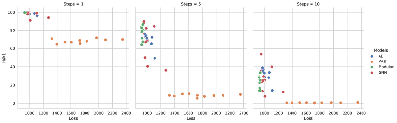
4.3 Prediction Metrics and RL Performance

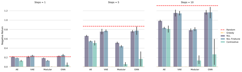
As discussed in Section 2.2, there are multiple evaluation metrics based on either prediction metrics or RL performance. The performance of the model on one metric may not necessarily transfer to another. We would like to analyze if this is the case for the models trained under various environments. We first note that while the ranking metrics were relatively good for most models on physics environments, most of them only did slightly better than a random policy on downstream RL, especially on larger graphs (Figures Figure 7 - 12 and Table 3 - 8 for ranking metrics; Figure 13 - 18 and Table 9 - 14 for downstream RL). Figures 21, 22 and 27 show scatter plots for each pair of losses, with one loss on each axis. While there is some correlation between ranking metric and RL performance (Modular and GNN; Figure 21), we did not find this trend to be consistent across models and environment settings. We feel that these results give further evidence of need to evaluate on RL performance.

4.4 Training objectives and learning

Likelihood loss and contrastive loss (Oord et al., 2018; Kipf et al., 2019) are two frequently used objectives for training world models in MBRL. We trained the models under each of these objective functions to understand how they impact learning. In almost all cases, models with explicit structure (modular models and GNNs) trained on contrastive loss perform better in terms of ranking loss compared to those trained on likelihood loss (refer to Figure 7 - 12). We don’t see a very clear trend between training objective and downstream RL performance but we do see a few cases where contrastively trained models performed much better than others (refer to Figures 6, 13, 17 and 18 and Tables 9, 13 and 14).

For other key insights and experimental conclusions on different environments, we refer the readers to Section F.6 for the physics environment and Section G.3 for the chemistry environment.

5 Related work

Video Prediction and Visual Question Answering. There exist a number of video prediction (Yi et al., 2019; Baradel et al., 2019) and visual question answering (Johnson et al., 2017) datasets that also make use of a blocks world for visual representation. Though these datasets can appear visually similar to ours at first glance, they lack two essential ingredients for systematically evaluating models for causal induction in MBRL. The first is that they do not allow active interventions and hence make it challenging for evaluating model-based reinforcement learning algorithms. Another key point is that these environments do not allow one to systematically perturb different aspects of causal graphs, hence, preventing to systematically study the performances of models for causal induction.

RL Environments. There exist several benchmarks for multi-task learning for robotics (Meta-World (Yu et al., 2019) and RLBench (James et al., 2020)) and for video gaming domain (Arcade Learning Environment, CoinRun (Cobbe et al., 2018), Sonic Benchmark (Machado et al., 2018), MazeBase (Nichol et al., 2018) and BabyAI (Chevalier-Boisvert et al., 2018)). However, as mentioned earlier, these benchmarks do not allow one to systematically control different aspects of causal models (such as the structure, the sparsity of edges and the size of the graph), hence making it difficult to systematically study causal induction in MBRL. The Alchemy (Wang et al., 2021) environment, which was released earlier this year, moves a step towards causal induction for meta-RL. Though the environment allows for some level of control of the underlying causal structures of the environment, it still does so in a limited way.

Block World. The AI community has been using the “blocks world” for decades as a testbed for various AI problems, including learning theory (Winston, 1970), natural language (Winograd, 1972), and planning (Fahlman, 1974). Block world allows to easily vary different aspects of the underlying causal structure, and also allow interventions to be performed on many high level variables of the environment giving rise to a large space of tasks which have well-defined relations between them.

6 Discussions and conclusions

In our work, we focus on studying various model-based approaches for causal induction in model-based RL. We highlighted the limitations of existing benchmarks and introduced a novel suite of environments that can help measure progress and facilitate research in this direction. We evaluated various models under many different settings and discuss the essential problems and challenges in combining both fields i.e ingredients, that we believe are common in the real world, such as modular factorization of the objects and interactions of objects governed by some unknown rules. Using a proposed evaluation framework, we demonstrate that structural inductive biases are beneficial to learning causal relationships and yield significantly improved performances in learning world models. We hope that our work helps to facilitate future work for understanding causal relationships in model-based reinforcement learning.

Acknowledgements

The authors would like to acknowledge the support of the following agencies for research funding and computing support: NSERC, Compute Canada, the Canada Research Chairs, CIFAR. We would also like to thank the developers of Pytorch for developments of great frameworks. We would like to thank Dmitriy Serdyuk for useful feedback and discussions.

References

Baradel et al. [2019] Fabien Baradel, Natalia Neverova, Julien Mille, Greg Mori, and Christian Wolf. Cophy: Counterfactual learning of physical dynamics. arXiv preprint arXiv:1909.12000, 2019.
Battaglia et al. [2016] Peter Battaglia, Razvan Pascanu, Matthew Lai, Danilo Jimenez Rezende, et al. Interaction networks for learning about objects, relations and physics. In Advances in neural information processing systems, pages 4502–4510, 2016.
Battaglia et al. [2018] Peter W Battaglia, Jessica B Hamrick, Victor Bapst, Alvaro Sanchez-Gonzalez, Vinicius Zambaldi, Mateusz Malinowski, Andrea Tacchetti, David Raposo, Adam Santoro, Ryan Faulkner, et al. Relational inductive biases, deep learning, and graph networks. arXiv preprint arXiv:1806.01261, 2018.
Bengio et al. [2019] Yoshua Bengio, Tristan Deleu, Nasim Rahaman, Rosemary Ke, Sébastien Lachapelle, Olexa Bilaniuk, Anirudh Goyal, and Christopher Pal. A meta-transfer objective for learning to disentangle causal mechanisms. arXiv preprint arXiv:1901.10912, 2019.
Chevalier-Boisvert et al. [2018] Maxime Chevalier-Boisvert, Dzmitry Bahdanau, Salem Lahlou, Lucas Willems, Chitwan Saharia, Thien Huu Nguyen, and Yoshua Bengio. Babyai: A platform to study the sample efficiency of grounded language learning. In International Conference on Learning Representations, 2018.
Cobbe et al. [2018] Karl Cobbe, Oleg Klimov, Chris Hesse, Taehoon Kim, and John Schulman. Quantifying generalization in reinforcement learning. arXiv preprint arXiv:1812.02341, 2018.
Dasgupta et al. [2019] Ishita Dasgupta, Jane Wang, Silvia Chiappa, Jovana Mitrovic, Pedro Ortega, David Raposo, Edward Hughes, Peter Battaglia, Matthew Botvinick, and Zeb Kurth-Nelson. Causal reasoning from meta-reinforcement learning. arXiv preprint arXiv:1901.08162, 2019.
de Haan et al. [2019] Pim de Haan, Dinesh Jayaraman, and Sergey Levine. Causal confusion in imitation learning. In Advances in Neural Information Processing Systems, pages 11698–11709, 2019.
Eaton and Murphy [2007] Daniel Eaton and Kevin Murphy. Exact bayesian structure learning from uncertain interventions. In Artificial Intelligence and Statistics, pages 107–114, 2007.
Fahlman [1974] Scott Elliott Fahlman. A planning system for robot construction tasks. Artificial intelligence, 5(1):1–49, 1974.
Gilmer et al. [2017] Justin Gilmer, Samuel S Schoenholz, Patrick F Riley, Oriol Vinyals, and George E Dahl. Neural message passing for quantum chemistry. In Proceedings of the 34th International Conference on Machine Learning-Volume 70, pages 1263–1272. JMLR. org, 2017.
Goyal and Bengio [2020] Anirudh Goyal and Yoshua Bengio. Inductive biases for deep learning of higher-level cognition. arXiv preprint arXiv:2011.15091, 2020.
Goyal et al. [2019] Anirudh Goyal, Alex Lamb, Jordan Hoffmann, Shagun Sodhani, Sergey Levine, Yoshua Bengio, and Bernhard Schölkopf. Recurrent independent mechanisms. arXiv preprint arXiv:1909.10893, 2019.
Goyal et al. [2020] Anirudh Goyal, Alex Lamb, Phanideep Gampa, Philippe Beaudoin, Sergey Levine, Charles Blundell, Yoshua Bengio, and Michael Mozer. Object files and schemata: Factorizing declarative and procedural knowledge in dynamical systems. arXiv preprint arXiv:2006.16225, 2020.
Ha and Schmidhuber [2018] David Ha and Jürgen Schmidhuber. World models. arXiv preprint arXiv:1803.10122, 2018.
James et al. [2020] Stephen James, Zicong Ma, David Rovick Arrojo, and Andrew J Davison. Rlbench: The robot learning benchmark & learning environment. IEEE Robotics and Automation Letters, 5(2):3019–3026, 2020.
Johnson et al. [2017] Justin Johnson, Bharath Hariharan, Laurens van der Maaten, Li Fei-Fei, C Lawrence Zitnick, and Ross Girshick. Clevr: A diagnostic dataset for compositional language and elementary visual reasoning. In Proceedings of the IEEE Conference on Computer Vision and Pattern Recognition, pages 2901–2910, 2017.
Ke et al. [2019] Nan Rosemary Ke, Olexa Bilaniuk, Anirudh Goyal, Stefan Bauer, Hugo Larochelle, Chris Pal, and Yoshua Bengio. Learning neural causal models from unknown interventions. arXiv preprint arXiv:1910.01075, 2019.
Ke et al. [2020] Nan Rosemary Ke, Jane Wang, Jovana Mitrovic, Martin Szummer, Danilo J Rezende, et al. Amortized learning of neural causal representations. arXiv preprint arXiv:2008.09301, 2020.
Kingma and Ba [2014] Diederik P Kingma and Jimmy Ba. Adam: A method for stochastic optimization. arXiv preprint arXiv:1412.6980, 2014.
Kingma and Welling [2013] Diederik P Kingma and Max Welling. Auto-encoding variational bayes. arXiv preprint arXiv:1312.6114, 2013.
Kipf et al. [2019] Thomas Kipf, Elise van der Pol, and Max Welling. Contrastive learning of structured world models. arXiv preprint arXiv:1911.12247, 2019.
Machado et al. [2018] Marlos C Machado, Marc G Bellemare, Erik Talvitie, Joel Veness, Matthew Hausknecht, and Michael Bowling. Revisiting the arcade learning environment: Evaluation protocols and open problems for general agents. Journal of Artificial Intelligence Research, 61:523–562, 2018.
Mittal et al. [2020] Sarthak Mittal, Alex Lamb, Anirudh Goyal, Vikram Voleti, Murray Shanahan, Guillaume Lajoie, Michael Mozer, and Yoshua Bengio. Learning to combine top-down and bottom-up signals in recurrent neural networks with attention over modules. arXiv preprint arXiv:2006.16981, 2020.
Nair et al. [2019] Suraj Nair, Yuke Zhu, Silvio Savarese, and Li Fei-Fei. Causal induction from visual observations for goal directed tasks. arXiv preprint arXiv:1910.01751, 2019.
Nichol et al. [2018] Alex Nichol, Vicki Pfau, Christopher Hesse, Oleg Klimov, and John Schulman. Gotta learn fast: A new benchmark for generalization in rl. arXiv preprint arXiv:1804.03720, 2018.
Oord et al. [2018] Aaron van den Oord, Yazhe Li, and Oriol Vinyals. Representation learning with contrastive predictive coding. arXiv preprint arXiv:1807.03748, 2018.
Osband et al. [2019] Ian Osband, Yotam Doron, Matteo Hessel, John Aslanides, Eren Sezener, Andre Saraiva, Katrina McKinney, Tor Lattimore, Csaba Szepezvari, Satinder Singh, et al. Behaviour suite for reinforcement learning. arXiv preprint arXiv:1908.03568, 2019.
Pearl [2009] Judea Pearl. Causality. Cambridge university press, 2009.
Peters et al. [2016] Jonas Peters, Peter Bühlmann, and Nicolai Meinshausen. Causal inference by using invariant prediction: identification and confidence intervals. Journal of the Royal Statistical Society: Series B (Statistical Methodology), 78(5):947–1012, 2016.
Peters et al. [2017] Jonas Peters, Dominik Janzing, and Bernhard Schölkopf. Elements of causal inference: foundations and learning algorithms. MIT press, 2017.
Rezende et al. [2020] Danilo J Rezende, Ivo Danihelka, George Papamakarios, Nan Rosemary Ke, Ray Jiang, Theophane Weber, Karol Gregor, Hamza Merzic, Fabio Viola, Jane Wang, et al. Causally correct partial models for reinforcement learning. arXiv preprint arXiv:2002.02836, 2020.
Rezende et al. [2014] Danilo Jimenez Rezende, Shakir Mohamed, and Daan Wierstra. Stochastic backpropagation and approximate inference in deep generative models. In Proceedings of The 31st International Conference on Machine Learning, pages 1278–1286, 2014.
Schölkopf et al. [2021] Bernhard Schölkopf, Francesco Locatello, Stefan Bauer, Nan Rosemary Ke, Nal Kalchbrenner, Anirudh Goyal, and Yoshua Bengio. Toward causal representation learning. Proceedings of the IEEE, 109(5):612–634, 2021.
Schrittwieser et al. [2019] Julian Schrittwieser, Ioannis Antonoglou, Thomas Hubert, Karen Simonyan, Laurent Sifre, Simon Schmitt, Arthur Guez, Edward Lockhart, Demis Hassabis, Thore Graepel, et al. Mastering atari, go, chess and shogi by planning with a learned model. arXiv preprint arXiv:1911.08265, 2019.
Silver and Ciosek [2012] David Silver and Kamil Ciosek. Compositional planning using optimal option models. arXiv preprint arXiv:1206.6473, 2012.
Sutton [1991] Richard S Sutton. Dyna, an integrated architecture for learning, planning, and reacting. ACM Sigart Bulletin, 2(4):160–163, 1991.
Tacchetti et al. [2018] Andrea Tacchetti, H Francis Song, Pedro AM Mediano, Vinicius Zambaldi, Neil C Rabinowitz, Thore Graepel, Matthew Botvinick, and Peter W Battaglia. Relational forward models for multi-agent learning. arXiv preprint arXiv:1809.11044, 2018.
Van Steenkiste et al. [2018] Sjoerd Van Steenkiste, Michael Chang, Klaus Greff, and Jürgen Schmidhuber. Relational neural expectation maximization: Unsupervised discovery of objects and their interactions. arXiv preprint arXiv:1802.10353, 2018.
Veerapaneni et al. [2020] Rishi Veerapaneni, John D Co-Reyes, Michael Chang, Michael Janner, Chelsea Finn, Jiajun Wu, Joshua Tenenbaum, and Sergey Levine. Entity abstraction in visual model-based reinforcement learning. In Conference on Robot Learning, pages 1439–1456. PMLR, 2020.
Wang et al. [2021] Jane X Wang, Michael King, Nicolas Porcel, Zeb Kurth-Nelson, Tina Zhu, Charlie Deck, Peter Choy, Mary Cassin, Malcolm Reynolds, Francis Song, et al. Alchemy: A structured task distribution for meta-reinforcement learning. arXiv preprint arXiv:2102.02926, 2021.
Watters et al. [2019] Nicholas Watters, Loic Matthey, Matko Bosnjak, Christopher P Burgess, and Alexander Lerchner. Cobra: Data-efficient model-based rl through unsupervised object discovery and curiosity-driven exploration. arXiv preprint arXiv:1905.09275, 2019.
Winograd [1972] Terry Winograd. Understanding natural language. Cognitive psychology, 3(1):1–191, 1972.
Winston [1970] Patrick H Winston. Learning structural descriptions from examples. 1970.
Yi et al. [2019] Kexin Yi, Chuang Gan, Yunzhu Li, Pushmeet Kohli, Jiajun Wu, Antonio Torralba, and Joshua B Tenenbaum. Clevrer: Collision events for video representation and reasoning. arXiv preprint arXiv:1910.01442, 2019.
Yu et al. [2019] Tianhe Yu, Deirdre Quillen, Zhanpeng He, Ryan Julian, Karol Hausman, Chelsea Finn, and Sergey Levine. Meta-world: A benchmark and evaluation for multi-task and meta reinforcement learning. arXiv preprint arXiv:1910.10897, 2019.
Zheng et al. [2018] Xun Zheng, Bryon Aragam, Pradeep K Ravikumar, and Eric P Xing. DAGs with NO TEARS: Continuous optimization for structure learning. In Advances in Neural Information Processing Systems, pages 9472–9483, 2018.

Part I Appendix

Appendix A Dataset Documentation

We open-source our environment, data, code and instructions on how to run them ¹¹1https://github.com/dido1998/CausalMBRL. We do not provide the data as a downloadable file, it can be generated using the instructions in the repository. We provide instructions to reproduce the results of our benchmark experiments. The data is provided under the MIT license. We bear all responsibility in-case the dataset leads to any violation of rights. The metadata for the dataset can also be found in the given github repository.

Intended Use. The intended use of this dataset is for causal learning research in model-based RL. We hope that this dataset can help to speed up discovery of novel methods that can learn causal relations in RL environments.

Reading the Data. The data is generated and stored in HDF5 format. ²²2https://www.hdfgroup.org/solutions/hdf5/, it can be accessed using the h5py python package ³³3https://pypi.org/project/h5py/. We provide the code for reading the data.

Appendix B A short review to Structured Causal Models

Causal modeling.

A Structural Causal Model (SCM) [Peters et al., 2017] over a finite number $M$ of random variables $X_{i}$ is a function that maps from the jointly-independent noise $N_{i}$ and parents (direct causes) $X_{pa(i,C)}$ of $X_{i}$ to $X_{i}$ . The matrix $C\in\{0,1\}^{M\times M}$ represents the adjacency matrix (structure) of the graph, such that $c_{ij}=1$ if node $i$ has node $j$ as a parent (equivalently, $X_{j}\in X_{pa(i,C)}$ ; i.e. $X_{j}$ is a direct cause of $X_{i}$ ).

\displaystyle X_{i}

\displaystyle:=f_{i}(X_{pa(i,C)},N_{i})\;,\quad\forall i\in\{0,\ldots,M-1\}

(1)

Causal structure discovery is the recovery of ground-truth $C$ from observational and/or interventional studies.

Interventions.

An intervention on a variable $X_{i}$ changes the function $f_{i}$ that maps from the causal parents of $X_{i}$ and the independent noise ( $(X_{pa(i,C)},N_{i})$ ) to $X_{i}$ . There are several common types of interventions available [Eaton and Murphy, 2007]: No intervention: only observational data is obtained from the ground truth model. Perfect: the value of a single or several variables is fixed and then ancestral sampling is performed on the other variables. Imperfect: the conditional distribution of the variable on which the intervention is performed is changed. All our experiments are performed with perfect interventions (aka. setting the state of a variable to a particular value, for example location or color), as they are the most common type of interventions in RL.

Appendix C Ranking based Evaluation

Apart from standard reconstruction loss, we also provide ranking results based on the evaluation metrics followed by Kipf et al. [2019]. Given observations at two different time steps, these metrics capture how close is the predicted transition in the embedding space to the embedding of the true observation obtained through the true environment transitions. Here the notion of closeness is defined as ranking from a large buffer of states under euclidean norm.

C.1 Hits at Rank 1 (H@1)

This score is 1 for a particular example if the predicted state representation is nearest to the encoded true observation and 0 otherwise. Thus, it measures whether the rank of the predicted representation is equal to 1 or not, where ranking is done over all reference state representations by distance to the true state representation. We report the average of this score over the test set.

C.2 Mean Reciprocal Rank (MRR)

This is defined as the average inverse rank, i.e, MRR $=\frac{1}{N}\sum_{n=1}^{N}\frac{1}{\text{rank}_{n}}$ where $\text{rank}_{n}$ is the rank of the $n^{th}$ sample of the test set where ranking is done over all reference state representations.

Appendix D Reward Prediction Evaluation

Below, we provide the methodology of training the reward predictor and doing evaluation based on it as well as further implementation details relevant to our particular set of environments.

D.1 Methodology

For downstream RL evaluation, we consider learning a reward predictor and then performing planning based on taking greedy actions in the direction of immediate highest reward (inspired from Watters et al. [2019]). For our tasks, the reward is a function of the next state and the target state but not the action. For example, in physics environment the reward is the average distance between the objects in their current configuration and a target configuration. Similarly, for chemistry environment it is the number of color matches between the current state and the target state.

More concretely, we learn a reward predictor function (parameterized by a single layered MLP) that takes as input the current state as well as the target state of the world and tries to predict the reward for the current state. This reward predictor is learned in a supervised way and all the other weights (encoder, decoder, transition models) are kept fixed during this training. Thus, it is only possible to learn a good reward predictor if the encoder model captures the important aspects of the objects from the raw image.

Given the current encoded state of the world, we consider all possible actions and transitions according to them in the latent space (using the learned transition model). After the transition, we use the learned reward predictor to predict the reward for the (new state, target state) pair. This gives us the immediate reward obtained from each action. Having obtained those rewards, our policy is to just greedily take the action that gives us the best immediate reward. Note that in our reward setting (dense and/or partial rewards) this is typically a good policy as can be seen in the oracle (greedy) performance (where we take actions according to the true reward).

For training, we consider the supervised $L_{1}$ loss optimized using the Adam Optimizer -

	$\displaystyle\mathcal{L}_{Reward\;Predictor}(\theta)$	$\displaystyle=\lVert f_{\theta}(s_{t},s_{target})-r(x_{t},x_{target})\rVert_{1}$
	$\displaystyle s_{t}$	$\displaystyle=\text{Encoder}(x_{t})$
	$\displaystyle s_{target}$	$\displaystyle=\text{Encoder}(x_{target})$

where $r(\cdot,\cdot)$ is the true reward function.

For evaluation, we consider the true final reward as well as the success rate obtained under policy $\pi$ where $\pi$ is implicitly defined using the learned reward function $f_{\theta}$ as follows -

\displaystyle\pi(s_{t},s_{target})

\displaystyle=\operatorname*{arg\,max}_{a\in\mathcal{A}}f_{\theta}(\text{Transition}(s_{t},a),s_{target})

We leave the formulation of training a value function estimator using a TD-learning objective as an important future work.

D.2 Implementation Details

For all the environments, when training a reward predictor we consider a starting state of the environment and the state of the environment obtained after doing 10 random actions. Given the starting state and the target state, we use the dense reward obtained in the configuration to act as the supervision signal for training of the reward predictor model.

For physics environment, we consider the reward to be the average distance of objects from their target configurations. Whereas, for the chemistry environment we consider the number of partial matches between the two states as the reward function.

For evaluation on downstream RL tasks, for $k^{th}$ step prediction, we consider targets that are generated from $k$ random actions in the environment. We also report baseline performances of a random policy as well as an optimal policy. For the physics environment, we set the optimal policy to be the one step greedy policy based on the true reward while for the chemistry environment, we consider the same actions that led to the target configuration to be the optimal policy. Note that since the chemistry environment is stochastic, the same actions may not lead to the same state. Hence any loss in performance even after performing optimal actions is due to the data uncertainty that arises due to the stochasticity.

Appendix E Model setups and training procedure

E.1 Model Based Experiments

For our model based experiments, we consider four models that encode different inductive biases -

•

Autoencoders (AE) - Monolithic model that compresses everything into a single entity.
•

Variational Autoencoders (VAE) - Similar to Autoencoders but with regularization to stay close to a prior distribution in latent space.
•

Modular Model (Modular) - Has a separate representation for each object and can be used to capture interactions between multiple sets of objects.
•

Graph Neural Networks (GNN) - Also has an object-wise representation but can capture only pairwise interactions between objects.

Each model has an encoder-decoder model as well as a transition model. The encoder-decoder model is aimed at inferring the high level causal variables from raw pixel data whereas the transition model is tasked with controlling how the encoded state transitions based on the actions taken. We build all our models on the architectural backbone provided by Kipf et al. [2019].

The encoder model is a convolutional neural network followed by a 3-layered MLP (Table 1). It outputs a single representation in case of monolithic models and an object-wise representation (i.e. separate for each object) in case of modular networks and graph neural networks.

The decoder model (if used - refer Section E.2) takes either a single representation (in case of monolithic models) or object-wise representations (in case of modular networks / GNNs) and outputs an image as close as possible to the input image. The structure of the decoder is detailed in Table 2.

We follow the medium encoder-decoder structure followed by Kipf et al. [2019]. For embedding dimension, we use a fixed embedding dimension of 32 per object where the number of objects are specified by the environment description. For example, if we have 3 objects in the environment, then the embedding dimension of Autoencoder based models is 96 while it is 32 per object for Modular/GNN models.

Mathematically, given an observation $x_{t}$ , the encoder maps the observation to its latent representation $s_{t}$ which is either monolithic or modular. Further, the decoder (if used) maps the latent representation back to the input space.

	$\displaystyle s_{t}$	$\displaystyle=\text{Encoder}(x_{t})$
	$\displaystyle\hat{x}_{t}$	$\displaystyle=\text{Decoder}(s_{t})$

Each architecture also has a transition model to model how a particular action affects the state of the world. Based on the current state of the world and an action taken, the transition model predicts the next state of the world. For monolithic models (AE and VAE), the transition model is a 3-layered MLP. For GNN, it is a graph neural network with only one node-to-edge and one edge-to-node information propagation, that is, it encodes only pairwise interactions. For modular models, it is a separate MLP for each object, that allows it to encode higher order interactions between multiple objects.

Mathematically, the transition (prediction of next state) from a given state $s_{t}$ based on an action $a_{t}$ can be shown as -

\displaystyle\hat{s}_{t+1}

\displaystyle=\text{Transition}(s_{t},a_{t})

Type	channels	activation	stride
Conv2D $9\times 9$	512	Leaky Relu	1
BatchNorm2D	-	-	-
Conv2D $5\times 5$	$M$ (number of objects)	Sigmoid	5

Table 1: Architecture of the encoder used for the world models.

Type	channels	activation	stride
Linear	512	Relu	-
Linear	512	Relu	-
Linear	$M\times 10\times 10$	-	-
ConvTranspose2D $5\times 5$	512	Relu	5
BatchNorm2D	-	-	-
ConvTranspose2D $9\times 9$	50	-	1

Table 2: Architecture of the decoder used for the world models.

E.2 Training Details

We consider two methods of training for all our baseline models -

•

Negative Log Likelihood (NLL)
•

Contrastive Loss (Decoder Free)

For the models trained using NLL, we perform training in 3 stages. First, we do pretraining where only the encoder and decoder are trained to reconstruct the given image. Second, we learn the transition where the encoder and decoder are fixed and the transition function is trained to optimally predict the next state given the current state and action. Finally, we do finetuning where we train both the encoder-decoder model as well as the transition model on combined objectives of reconstructing the current images, reconstructing the images in next step as well as doing correct transitions in the latent space.

For the reconstructions, we use the binary cross entropy loss (BCE loss) while for the transitions, we use the mean squared error loss (MSE loss).

Mathematically, given the current observation $x_{t}$ , the action taken $a_{t}$ and the next observation obtained $x_{t+1}$ , we first encode both the observations into the latent space as -

	$\displaystyle s_{t}$	$\displaystyle=\text{Encoder}(x_{t})$
	$\displaystyle s_{t+1}$	$\displaystyle=\text{Encoder}(x_{t+1})$

We then perform a transition from the current step using the transition model as well as use the decoder to perform reconstructions based on the current encoded state as well as the predicted state -

	$\displaystyle\hat{s}_{t+1}$	$\displaystyle=\text{Transition}(s_{t},a_{t})$
	$\displaystyle\hat{x}_{t}$	$\displaystyle=\text{Decoder}(s_{t})$
	$\displaystyle\hat{x}_{t+1}$	$\displaystyle=\text{Decoder}(\hat{s}_{t+1})$

Given these variables, the pretraining, transition training and the finetuning can be characterized as -

	Pretraining :	$\displaystyle\operatorname*{arg\,min}_{\text{Encoder},\text{Decoder}}\text{BCE}(x_{t},\hat{x}_{t})$
	Transition :	$\displaystyle\operatorname*{arg\,min}_{\text{Transition}}\text{MSE}(s_{t+1},\hat{s}_{t+1})$
	Finetuning :	$\displaystyle\operatorname*{arg\,min}_{\text{Encoder, Decoder, Transition}}\text{BCE}(x_{t},\hat{x}_{t})+\text{MSE}(s_{t+1},\hat{s}_{t+1})+\text{BCE}(x_{t+1},\hat{x}_{t+1})$

For models trained with contrastive loss, we follow the same setup as in Kipf et al. [2019]. In this setup we don’t use a decoder and instead learn everything in encoded state end-to-end. Mathematically, this can be described as the following -

	$\displaystyle\textit{Contrastive Training }:\operatorname*{arg\,min}_{\text{Encoder, Transition}}$	$\displaystyle H+\max(0,\gamma-\tilde{H})$
	$\displaystyle H$	$\displaystyle=\text{MSE}(\hat{s}_{t+1},s_{t+1})$
	$\displaystyle\tilde{H}$	$\displaystyle=\text{MSE}(\tilde{s}_{t+1},s_{t+1})$
	$\displaystyle\tilde{s}_{t+1}$	$\displaystyle:\text{ Negative state obtained from random shuffling of batch}$

We train each stage for 100 epochs using Adam optimizer [Kingma and Ba, 2014] with a learning rate of 5e-4 and batch size 512.

Appendix F Physics Environment

F.1 Detailed setups

We provide an environment which consists of objects of different shapes and potentially different colors. Each object has a unique weight associated with it and only heavier objects can push lighter ones. This induces an acyclic tournament causal graph with sparse two-way interactions between the objects, which form the nodes of the graph.

More precisely, the physics environment with $M$ objects (eg. 3) and colormap $C$ (eg. blues) can be considered as the set $\{o_{i}=\{s_{i},w_{i},c_{i},p_{i}\}\mid i=1\text{ to }M\}$ where $o_{i}$ denotes the $i^{th}$ object which is characterized by its position $p_{i}$ , its shape $s_{i}$ , its color $c_{i}$ and its weight $w_{i}$ . An edge exists from $o_{i}$ to $o_{j}$ if and only if $w_{i}>w_{j}$ . We consider the weight of each object to be unique, thereby getting rid of cycles. The specifics of the environment are determined by how the shape, color and weight of an object are related. For our experimentation, we consider two different settings which are outlined below. However, we emphasize that the physics environment is not limited to just these specifications and can be easily extended to form more complicated relationships between the three properties.

F.2 Identity of Objects

Since we are proposing RL environments, we need to make sure that the mapping from the action space to the object space is well defined and observable / learnable. Here, we briefly discuss that it is the case in the settings of the physics environment proposed in this paper. We also discuss that in the Unobserved environment this mapping can be very hard to learn and for this reason, we proposed another variant known as FixedUnobserved environment.

Our mapping from action space to object space is such that given an initialization of the environment, the first action dimension always corresponds to the heaviest object. Similarly, the second to the second heaviest and so on.

Now, in the Observed environment case, the heaviest object is also the darkest object in the scene so it is relatively easy for a model to infer the action to object mapping once it has learned the fact that intensity of color represents the weight of the object.

On the other hand, in the Unobserved case, the colors of the objects are sampled without replacement from a larger set of colors. For example, consider a 3 object environment with the set of colors to be red < green < orange < yellow where the ordering defines the ordering of the weight. Then if in one initialization has the colors (red, green, yellow) then here the first action dimension corresponds to the color red. However, another initialization of the same environment can be (green orange, yellow) and then the first action dimension would correspond to the green object. Thus, for a model to learn the action to object mapping, it has to learn this global ranking of colors. We found that this was typically hard for the models to do.

To alleviate the above complexity, we consider another setting FixedUnobserved where we keep the shapes of the objects fixed and unique. Here, there is an additional constraint that apart from the colors following a global ordering of weights, the unique shapes also follow a global ordering of weights and hence, this creates an easily learnable mapping.

F.3 All variables are observed

In this setting, we consider all the objects to be of the same color but different shades, eg. different shades of the color blue. The weight of each object is a monotonic function of its color intensity, meaning that darker objects are heavier.

Mathematically, given a colormap $C$ (single color; continuous in intensity of the color), $c_{i}\in[0,1]$ denotes the intensity of the color $C$ for object $i$ (1 being darkest; 0 lightest). Moreover, the weight of that object is given by $w_{i}=g(c_{i})$ , where g is a strictly monotonic function. Thus, darker objects are given heavier weights and thus can push lighter objects.

This setting easily allows for zero shot generalization since a model that has been trained on a subset of shades of a particular color can generalize to do well across different shades of the same color. Moreover, the shape of an object here is a distractor since the dynamics of the objects are only controlled by their colors.

F.4 Some variables are unobserved

In this setting, all objects are of distinct discrete colors drawn from a discrete colormap $c$ . Each color is associated with a unique weight and here, too, heavier objects can push lighter ones but not vice versa.

Mathematically, given a colormap $C$ (multiple discrete options), $c_{i}\in C$ denotes the color for object $i$ such that $c_{i}\neq c_{j}\;\forall i\neq j$ . Moreover, the weight of that object is given by $w_{i}=g(h_{i})$ , where g is an injective function and $g:C\to\mathbb{R}$ .

This setting does not allow for zero shot generalization in the colors since whenever a new color is introduced, the agent will have to perform interventions on it to infer its place in the graph. However, similar to the observed case, the shapes of the objects act as distractors since the dynamics is only controlled by the colors.

F.5 Unobserved Variables but Fixed Shapes

In this setting, all objects are of distinct discrete colors and shapes where the set of shapes is kept constant across different episodes. Here, the weight of an object can be reflected either from its shape or its color. For example, the lightest object in the episode will always be of a fixed unique shape and it will always have the lightest color (where lightest color is defined according to the order on the color in the colormap - eg. red < blue < green)

This setting does not allow for zero shot generalization in either the colors or the shapes since whenever a new color or shape is introduced, the agent will have to perform interventions on it to infer its place in the graph.

F.6 Experimental Results

We perform experiments on a wide range of settings for the underlying causal graph for the physics environment. We categorize our findings below -

•

Graph Neural Networks (GNNs) generally don’t perform well compared to Modular models and Autoencoders (AEs) on a wide variety of metrics (ranking metrics, reconstruction loss, downstream RL task) in the setting of likelihood based loss (refer to Figure 7 - Figure 18 and Table 3 - 14)
•

Models trained with contrastive loss are generally better at predictions made over longer time scales in terms of ranking metrics (refer to Figure 7 - 12 and Table 3 - 8)
•

Models trained with contrastive loss are also generally better at downstream RL tasks as compared to those trained with likelihood based loss. In particular there are some settings where the former were able to do almost perfect planning while the latter weren’t able to do good planning in any setting (refer to Figures 15, 17 and 18 and Tables 9, 13 and 14)
•

Modular models and Graph Neural Networks scale better than the monolithic counterparts when the number of objects in the causal graph increases. Further, while the ranking metrics still remain good, we see that the planning metrics suffer by a large margin (refer to Figure 7 - 18 and Table 3 - 14)
•

While Autoencoder models perform decently based on ranking metrics, they generally don’t perform as well on downstream RL tasks when compared to Graph Neural Networks and Modular models (refer to Figure 13 - 18 and Table 9 - 14)
•

While ranking metrics on the unobserved environment are still decent (refer to Figures 9 and 10 and Tables 5 and 6), we see that in terms of downstream RL planning, none of the models do much better than a random policy (refer to Figures 15 and 16 and Figures 15 and 16)
•

We see a case where models that have very good ranking metrics over long time horizons (AE with NLL Finetune; Figure 11 and Figure 17) perform much worse on downstream RL tasks than GNNs and Modular models which had lower ranking metrics (Table 13 and Figure 17).

		1 Step			5 Steps			10 Steps
	Model	H@1	MRR	Rec.	H@1	MRR	Rec.	H@1	MRR	Rec.
NLL	AE	97.23_{$\pm$ 0.37}	98.23_{$\pm$ 0.28}	0.04_{$\pm$ 0.0}	72.78_{$\pm$ 2.5}	77.74_{$\pm$ 2.14}	0.1_{$\pm$ 0.01}	40.46_{$\pm$ 3.48}	47.4_{$\pm$ 3.37}	0.22_{$\pm$ 0.01}
	GNN	64.86_{$\pm$ 4.43}	73.39_{$\pm$ 4.08}	0.11_{$\pm$ 0.01}	17.73_{$\pm$ 6.15}	25.44_{$\pm$ 7.73}	0.33_{$\pm$ 0.05}	6.4_{$\pm$ 3.51}	11.05_{$\pm$ 5.17}	0.44_{$\pm$ 0.06}
	Modular	97.13_{$\pm$ 0.55}	98.22_{$\pm$ 0.42}	0.04_{$\pm$ 0.0}	70.7_{$\pm$ 9.01}	76.46_{$\pm$ 7.95}	0.13_{$\pm$ 0.02}	36.66_{$\pm$ 9.88}	44.25_{$\pm$ 10.14}	0.26_{$\pm$ 0.03}
	VAE	49.52_{$\pm$ 1.51}	58.98_{$\pm$ 1.79}	0.25_{$\pm$ 0.02}	1.7_{$\pm$ 0.13}	3.4_{$\pm$ 0.16}	1.0_{$\pm$ 0.11}	0.16_{$\pm$ 0.03}	0.56_{$\pm$ 0.06}	1.18_{$\pm$ 0.14}
NLL Finetuned	AE	98.08_{$\pm$ 0.2}	98.81_{$\pm$ 0.15}	0.03_{$\pm$ 0.0}	80.95_{$\pm$ 2.2}	84.54_{$\pm$ 1.86}	0.07_{$\pm$ 0.0}	51.98_{$\pm$ 4.12}	57.96_{$\pm$ 3.84}	0.16_{$\pm$ 0.01}
	GNN	74.64_{$\pm$ 11.03}	78.88_{$\pm$ 10.19}	0.04_{$\pm$ 0.0}	32.43_{$\pm$ 16.24}	39.39_{$\pm$ 17.45}	0.14_{$\pm$ 0.05}	8.23_{$\pm$ 7.15}	12.03_{$\pm$ 9.29}	0.28_{$\pm$ 0.07}
	Modular	98.16_{$\pm$ 0.49}	99.0_{$\pm$ 0.33}	0.03_{$\pm$ 0.0}	81.49_{$\pm$ 10.07}	86.17_{$\pm$ 8.66}	0.07_{$\pm$ 0.02}	48.7_{$\pm$ 16.19}	56.48_{$\pm$ 16.41}	0.17_{$\pm$ 0.04}
	VAE	77.61_{$\pm$ 16.75}	83.27_{$\pm$ 13.68}	0.04_{$\pm$ 0.0}	18.96_{$\pm$ 13.9}	25.5_{$\pm$ 17.07}	0.29_{$\pm$ 0.08}	1.3_{$\pm$ 1.08}	2.87_{$\pm$ 1.96}	0.51_{$\pm$ 0.07}
Contrastive	AE	82.11_{$\pm$ 2.22}	88.5_{$\pm$ 1.61}	-	50.0_{$\pm$ 6.43}	65.2_{$\pm$ 5.04}	-	34.36_{$\pm$ 8.42}	51.22_{$\pm$ 8.17}	-
	GNN	93.86_{$\pm$ 9.59}	95.99_{$\pm$ 6.42}	-	78.28_{$\pm$ 32.39}	82.29_{$\pm$ 26.85}	-	72.06_{$\pm$ 39.58}	75.46_{$\pm$ 35.65}	-
	Modular	98.73_{$\pm$ 1.04}	99.31_{$\pm$ 0.58}	-	94.7_{$\pm$ 4.2}	97.02_{$\pm$ 2.38}	-	90.6_{$\pm$ 6.87}	94.45_{$\pm$ 4.08}	-

Table 3: Hits at Rank 1 (H@1), Mean Reciprocal Rank (MRR) (higher is better) and Reconstruction Error (lower is better) for different models and training losses for 1, 5 and 10 step prediction for the Observed Physics environment setting with 3 objects.

		1 Step			5 Steps			10 Steps
	Model	H@1	MRR	Rec.	H@1	MRR	Rec.	H@1	MRR	Rec.
NLL	AE	97.77_{$\pm$ 1.45}	98.38_{$\pm$ 1.05}	0.08_{$\pm$ 0.01}	63.88_{$\pm$ 9.77}	69.55_{$\pm$ 9.0}	0.25_{$\pm$ 0.03}	27.18_{$\pm$ 7.09}	33.6_{$\pm$ 7.71}	0.45_{$\pm$ 0.03}
	GNN	95.13_{$\pm$ 3.02}	96.95_{$\pm$ 2.24}	0.19_{$\pm$ 0.02}	41.49_{$\pm$ 3.95}	50.63_{$\pm$ 3.93}	0.47_{$\pm$ 0.05}	19.28_{$\pm$ 2.57}	26.59_{$\pm$ 3.06}	0.63_{$\pm$ 0.07}
	Modular	99.57_{$\pm$ 0.16}	99.73_{$\pm$ 0.12}	0.09_{$\pm$ 0.0}	79.14_{$\pm$ 4.89}	84.06_{$\pm$ 4.09}	0.28_{$\pm$ 0.01}	35.68_{$\pm$ 6.99}	43.82_{$\pm$ 7.55}	0.48_{$\pm$ 0.02}
	VAE	79.35_{$\pm$ 0.48}	84.38_{$\pm$ 0.4}	0.34_{$\pm$ 0.01}	6.18_{$\pm$ 1.76}	10.68_{$\pm$ 2.25}	1.62_{$\pm$ 0.1}	0.28_{$\pm$ 0.09}	0.97_{$\pm$ 0.22}	2.21_{$\pm$ 0.13}
NLL Finetuned	AE	98.29_{$\pm$ 0.77}	98.78_{$\pm$ 0.53}	0.07_{$\pm$ 0.01}	69.58_{$\pm$ 7.23}	74.59_{$\pm$ 6.45}	0.2_{$\pm$ 0.02}	31.75_{$\pm$ 6.64}	38.22_{$\pm$ 6.97}	0.39_{$\pm$ 0.02}
	GNN	97.71_{$\pm$ 2.81}	98.43_{$\pm$ 2.13}	0.07_{$\pm$ 0.0}	68.36_{$\pm$ 18.69}	73.78_{$\pm$ 17.13}	0.2_{$\pm$ 0.05}	26.52_{$\pm$ 13.33}	32.94_{$\pm$ 14.63}	0.46_{$\pm$ 0.13}
	Modular	99.65_{$\pm$ 0.2}	99.77_{$\pm$ 0.14}	0.06_{$\pm$ 0.0}	77.21_{$\pm$ 6.81}	82.08_{$\pm$ 5.83}	0.21_{$\pm$ 0.04}	23.15_{$\pm$ 6.27}	29.24_{$\pm$ 7.12}	0.53_{$\pm$ 0.12}
	VAE	68.44_{$\pm$ 2.1}	74.52_{$\pm$ 1.6}	0.09_{$\pm$ 0.0}	8.42_{$\pm$ 1.32}	12.42_{$\pm$ 1.8}	0.75_{$\pm$ 0.03}	0.58_{$\pm$ 0.14}	1.34_{$\pm$ 0.28}	1.07_{$\pm$ 0.05}
Contrastive	AE	96.12_{$\pm$ 1.73}	97.71_{$\pm$ 1.12}	-	67.36_{$\pm$ 20.12}	76.98_{$\pm$ 15.6}	-	44.65_{$\pm$ 32.39}	55.38_{$\pm$ 29.98}	-
	GNN	99.28_{$\pm$ 0.53}	99.6_{$\pm$ 0.31}	-	78.85_{$\pm$ 7.5}	84.81_{$\pm$ 6.21}	-	50.1_{$\pm$ 9.94}	60.25_{$\pm$ 10.11}	-
	Modular	99.71_{$\pm$ 0.13}	99.84_{$\pm$ 0.08}	-	84.3_{$\pm$ 2.84}	89.35_{$\pm$ 2.26}	-	52.36_{$\pm$ 4.02}	63.28_{$\pm$ 4.28}	-

Table 4: Hits at Rank 1 (H@1), Mean Reciprocal Rank (MRR) (higher is better) and Reconstruction Error (lower is better) for different models and training losses for 1, 5 and 10 step prediction for the Observed Physics environment setting with 5 objects.

		1 Step			5 Steps			10 Steps
	Model	H@1	MRR	Rec.	H@1	MRR	Rec.	H@1	MRR	Rec.
NLL	AE	65.69_{$\pm$ 1.93}	73.4_{$\pm$ 1.66}	0.12_{$\pm$ 0.0}	17.98_{$\pm$ 0.95}	25.84_{$\pm$ 1.15}	0.3_{$\pm$ 0.01}	6.56_{$\pm$ 0.6}	11.64_{$\pm$ 0.98}	0.39_{$\pm$ 0.02}
	GNN	62.27_{$\pm$ 3.7}	70.16_{$\pm$ 3.5}	0.15_{$\pm$ 0.01}	19.32_{$\pm$ 1.64}	26.2_{$\pm$ 2.14}	0.34_{$\pm$ 0.02}	8.87_{$\pm$ 1.35}	14.09_{$\pm$ 2.03}	0.42_{$\pm$ 0.02}
	Modular	75.23_{$\pm$ 2.69}	82.73_{$\pm$ 2.01}	0.12_{$\pm$ 0.0}	24.93_{$\pm$ 2.64}	33.96_{$\pm$ 3.08}	0.31_{$\pm$ 0.01}	10.39_{$\pm$ 1.67}	16.71_{$\pm$ 2.31}	0.39_{$\pm$ 0.01}
	VAE	52.83_{$\pm$ 1.98}	61.68_{$\pm$ 1.85}	0.28_{$\pm$ 0.01}	1.96_{$\pm$ 0.16}	3.92_{$\pm$ 0.26}	0.88_{$\pm$ 0.05}	0.19_{$\pm$ 0.04}	0.62_{$\pm$ 0.03}	1.0_{$\pm$ 0.07}
NLL Finetuned	AE	95.35_{$\pm$ 1.13}	97.02_{$\pm$ 0.75}	0.06_{$\pm$ 0.0}	40.92_{$\pm$ 7.81}	49.77_{$\pm$ 7.94}	0.21_{$\pm$ 0.02}	9.41_{$\pm$ 4.36}	13.92_{$\pm$ 5.64}	0.35_{$\pm$ 0.03}
	GNN	74.19_{$\pm$ 5.88}	80.08_{$\pm$ 5.04}	0.07_{$\pm$ 0.0}	20.13_{$\pm$ 8.28}	26.32_{$\pm$ 9.43}	0.16_{$\pm$ 0.01}	2.3_{$\pm$ 2.97}	3.94_{$\pm$ 4.06}	0.25_{$\pm$ 0.02}
	Modular	94.92_{$\pm$ 1.84}	96.79_{$\pm$ 1.24}	0.07_{$\pm$ 0.0}	27.62_{$\pm$ 6.53}	34.7_{$\pm$ 7.51}	0.21_{$\pm$ 0.02}	2.52_{$\pm$ 1.21}	4.16_{$\pm$ 1.74}	0.32_{$\pm$ 0.03}
	VAE	49.65_{$\pm$ 4.14}	59.58_{$\pm$ 3.92}	0.07_{$\pm$ 0.0}	7.82_{$\pm$ 1.04}	12.3_{$\pm$ 1.48}	0.25_{$\pm$ 0.03}	0.83_{$\pm$ 0.16}	2.05_{$\pm$ 0.29}	0.36_{$\pm$ 0.04}
Contrastive	AE	89.77_{$\pm$ 3.3}	94.0_{$\pm$ 2.11}	-	37.57_{$\pm$ 9.15}	53.53_{$\pm$ 8.72}	-	13.87_{$\pm$ 7.64}	26.54_{$\pm$ 10.18}	-
	GNN	89.58_{$\pm$ 5.13}	93.4_{$\pm$ 3.42}	-	40.33_{$\pm$ 10.2}	50.14_{$\pm$ 10.19}	-	17.74_{$\pm$ 6.99}	25.67_{$\pm$ 8.26}	-
	Modular	96.55_{$\pm$ 3.09}	97.96_{$\pm$ 1.96}	-	62.15_{$\pm$ 12.59}	71.49_{$\pm$ 11.61}	-	31.02_{$\pm$ 10.94}	42.39_{$\pm$ 12.6}	-

Table 5: Hits at Rank 1 (H@1), Mean Reciprocal Rank (MRR) (higher is better) and Reconstruction Error (lower is better) for different models and training losses for 1, 5 and 10 step prediction for the Unobserved Physics environment setting with 3 objects.

		1 Step			5 Steps			10 Steps
	Model	H@1	MRR	Rec.	H@1	MRR	Rec.	H@1	MRR	Rec.
NLL	AE	89.49_{$\pm$ 0.68}	92.15_{$\pm$ 0.62}	0.15_{$\pm$ 0.0}	37.78_{$\pm$ 1.7}	45.92_{$\pm$ 1.78}	0.35_{$\pm$ 0.01}	15.04_{$\pm$ 1.74}	21.52_{$\pm$ 2.21}	0.46_{$\pm$ 0.01}
	GNN	95.76_{$\pm$ 2.07}	97.3_{$\pm$ 1.53}	0.17_{$\pm$ 0.01}	49.46_{$\pm$ 1.98}	57.92_{$\pm$ 2.14}	0.42_{$\pm$ 0.04}	28.5_{$\pm$ 2.54}	36.75_{$\pm$ 2.99}	0.54_{$\pm$ 0.05}
	Modular	98.19_{$\pm$ 1.26}	98.93_{$\pm$ 0.81}	0.15_{$\pm$ 0.01}	57.51_{$\pm$ 5.46}	66.3_{$\pm$ 5.16}	0.37_{$\pm$ 0.03}	31.67_{$\pm$ 4.13}	40.84_{$\pm$ 4.55}	0.49_{$\pm$ 0.04}
	VAE	77.21_{$\pm$ 3.91}	81.44_{$\pm$ 3.54}	0.33_{$\pm$ 0.01}	26.01_{$\pm$ 2.63}	32.41_{$\pm$ 2.79}	0.89_{$\pm$ 0.04}	9.18_{$\pm$ 1.03}	13.74_{$\pm$ 1.25}	1.18_{$\pm$ 0.07}
NLL Finetuned	AE	95.79_{$\pm$ 0.58}	97.27_{$\pm$ 0.43}	0.11_{$\pm$ 0.0}	27.77_{$\pm$ 1.72}	35.19_{$\pm$ 1.88}	0.22_{$\pm$ 0.01}	3.73_{$\pm$ 0.45}	5.92_{$\pm$ 0.57}	0.32_{$\pm$ 0.02}
	GNN	99.04_{$\pm$ 0.72}	99.43_{$\pm$ 0.44}	0.1_{$\pm$ 0.0}	58.45_{$\pm$ 7.06}	65.86_{$\pm$ 6.56}	0.2_{$\pm$ 0.01}	10.34_{$\pm$ 3.74}	15.38_{$\pm$ 4.81}	0.28_{$\pm$ 0.01}
	Modular	99.87_{$\pm$ 0.05}	99.93_{$\pm$ 0.03}	0.1_{$\pm$ 0.0}	42.15_{$\pm$ 9.03}	49.12_{$\pm$ 9.4}	0.22_{$\pm$ 0.01}	4.35_{$\pm$ 2.47}	6.32_{$\pm$ 3.35}	0.36_{$\pm$ 0.04}
	VAE	65.67_{$\pm$ 5.74}	72.42_{$\pm$ 5.11}	0.11_{$\pm$ 0.0}	15.62_{$\pm$ 3.52}	20.41_{$\pm$ 4.25}	0.3_{$\pm$ 0.02}	3.55_{$\pm$ 1.5}	5.57_{$\pm$ 2.15}	0.42_{$\pm$ 0.03}
Contrastive	AE	97.23_{$\pm$ 0.93}	98.38_{$\pm$ 0.54}	-	56.62_{$\pm$ 5.66}	68.68_{$\pm$ 4.46}	-	22.86_{$\pm$ 5.52}	35.88_{$\pm$ 6.53}	-
	GNN	99.67_{$\pm$ 0.21}	99.81_{$\pm$ 0.12}	-	82.52_{$\pm$ 6.75}	86.9_{$\pm$ 5.33}	-	55.12_{$\pm$ 11.8}	63.04_{$\pm$ 10.74}	-
	Modular	99.8_{$\pm$ 0.14}	99.89_{$\pm$ 0.08}	-	82.98_{$\pm$ 3.25}	87.44_{$\pm$ 2.72}	-	50.92_{$\pm$ 4.73}	59.51_{$\pm$ 4.65}	-

Table 6: Hits at Rank 1 (H@1), Mean Reciprocal Rank (MRR) (higher is better) and Reconstruction Error (lower is better) for different models and training losses for 1, 5 and 10 step prediction for the Unobserved Physics environment setting with 5 objects.

		1 Step			5 Steps			10 Steps
	Model	H@1	MRR	Rec.	H@1	MRR	Rec.	H@1	MRR	Rec.
NLL	AE	99.0_{$\pm$ 0.1}	99.44_{$\pm$ 0.06}	0.04_{$\pm$ 0.0}	95.0_{$\pm$ 0.41}	96.81_{$\pm$ 0.31}	0.06_{$\pm$ 0.0}	84.54_{$\pm$ 1.5}	89.24_{$\pm$ 1.2}	0.1_{$\pm$ 0.01}
	GNN	70.68_{$\pm$ 4.95}	79.43_{$\pm$ 4.13}	0.11_{$\pm$ 0.02}	23.82_{$\pm$ 7.74}	33.28_{$\pm$ 9.14}	0.27_{$\pm$ 0.05}	10.11_{$\pm$ 5.08}	16.65_{$\pm$ 6.91}	0.36_{$\pm$ 0.06}
	Modular	98.03_{$\pm$ 0.22}	98.84_{$\pm$ 0.17}	0.05_{$\pm$ 0.0}	88.12_{$\pm$ 2.65}	91.8_{$\pm$ 2.2}	0.08_{$\pm$ 0.01}	68.6_{$\pm$ 9.01}	76.12_{$\pm$ 7.96}	0.12_{$\pm$ 0.02}
	VAE	53.12_{$\pm$ 2.76}	63.42_{$\pm$ 2.58}	0.21_{$\pm$ 0.01}	2.2_{$\pm$ 0.24}	4.53_{$\pm$ 0.4}	0.61_{$\pm$ 0.05}	0.2_{$\pm$ 0.04}	0.82_{$\pm$ 0.08}	0.76_{$\pm$ 0.07}
NLL Finetuned	AE	99.24_{$\pm$ 0.08}	99.59_{$\pm$ 0.05}	0.04_{$\pm$ 0.0}	96.73_{$\pm$ 0.37}	98.02_{$\pm$ 0.22}	0.05_{$\pm$ 0.0}	90.56_{$\pm$ 1.0}	93.72_{$\pm$ 0.69}	0.07_{$\pm$ 0.0}
	GNN	75.16_{$\pm$ 12.45}	79.97_{$\pm$ 11.99}	0.05_{$\pm$ 0.0}	34.78_{$\pm$ 14.54}	42.8_{$\pm$ 16.43}	0.11_{$\pm$ 0.04}	12.76_{$\pm$ 7.38}	17.88_{$\pm$ 9.47}	0.21_{$\pm$ 0.07}
	Modular	98.76_{$\pm$ 0.15}	99.35_{$\pm$ 0.09}	0.04_{$\pm$ 0.0}	91.3_{$\pm$ 2.18}	94.54_{$\pm$ 1.63}	0.06_{$\pm$ 0.0}	66.7_{$\pm$ 7.96}	75.15_{$\pm$ 7.17}	0.1_{$\pm$ 0.01}
	VAE	68.53_{$\pm$ 13.05}	76.55_{$\pm$ 10.71}	0.05_{$\pm$ 0.0}	21.38_{$\pm$ 10.49}	29.76_{$\pm$ 12.17}	0.18_{$\pm$ 0.03}	1.72_{$\pm$ 1.0}	3.85_{$\pm$ 1.66}	0.29_{$\pm$ 0.04}
Contrastive	AE	77.67_{$\pm$ 10.51}	86.21_{$\pm$ 7.08}	-	53.49_{$\pm$ 23.05}	68.11_{$\pm$ 17.57}	-	43.65_{$\pm$ 26.31}	59.13_{$\pm$ 21.53}	-
	GNN	84.94_{$\pm$ 8.08}	90.1_{$\pm$ 5.62}	-	42.88_{$\pm$ 28.35}	51.75_{$\pm$ 24.48}	-	28.06_{$\pm$ 35.18}	34.19_{$\pm$ 32.68}	-
	Modular	88.42_{$\pm$ 6.43}	93.32_{$\pm$ 4.48}	-	71.54_{$\pm$ 17.3}	83.07_{$\pm$ 12.72}	-	66.07_{$\pm$ 20.34}	79.36_{$\pm$ 15.62}	-

Table 7: Hits at Rank 1 (H@1), Mean Reciprocal Rank (MRR) (higher is better) and Reconstruction Error (lower is better) for different models and training losses for 1, 5 and 10 step prediction for the FixedUnobserved Physics environment setting with 3 objects.

		1 Step			5 Steps			10 Steps
	Model	H@1	MRR	Rec.	H@1	MRR	Rec.	H@1	MRR	Rec.
NLL	AE	98.51_{$\pm$ 0.14}	98.85_{$\pm$ 0.09}	0.07_{$\pm$ 0.0}	84.3_{$\pm$ 1.58}	87.34_{$\pm$ 1.18}	0.16_{$\pm$ 0.0}	58.14_{$\pm$ 2.86}	64.57_{$\pm$ 2.51}	0.26_{$\pm$ 0.01}
	GNN	95.61_{$\pm$ 2.72}	97.13_{$\pm$ 2.01}	0.13_{$\pm$ 0.02}	53.89_{$\pm$ 11.58}	62.05_{$\pm$ 10.9}	0.32_{$\pm$ 0.05}	28.64_{$\pm$ 11.56}	36.96_{$\pm$ 12.45}	0.44_{$\pm$ 0.07}
	Modular	99.48_{$\pm$ 0.25}	99.63_{$\pm$ 0.21}	0.07_{$\pm$ 0.0}	94.13_{$\pm$ 1.31}	95.54_{$\pm$ 1.24}	0.15_{$\pm$ 0.01}	78.18_{$\pm$ 3.17}	82.76_{$\pm$ 2.95}	0.23_{$\pm$ 0.02}
	VAE	74.2_{$\pm$ 0.99}	78.72_{$\pm$ 0.98}	0.23_{$\pm$ 0.01}	22.18_{$\pm$ 0.93}	27.69_{$\pm$ 0.91}	0.63_{$\pm$ 0.04}	5.68_{$\pm$ 0.88}	9.0_{$\pm$ 1.0}	0.83_{$\pm$ 0.06}
NLL Finetuned	AE	99.18_{$\pm$ 0.16}	99.37_{$\pm$ 0.11}	0.07_{$\pm$ 0.0}	91.48_{$\pm$ 1.86}	93.19_{$\pm$ 1.41}	0.12_{$\pm$ 0.01}	73.28_{$\pm$ 3.92}	77.99_{$\pm$ 3.36}	0.2_{$\pm$ 0.02}
	GNN	95.86_{$\pm$ 3.39}	97.36_{$\pm$ 2.31}	0.06_{$\pm$ 0.0}	65.56_{$\pm$ 16.0}	71.71_{$\pm$ 14.42}	0.13_{$\pm$ 0.03}	35.26_{$\pm$ 20.76}	41.63_{$\pm$ 20.99}	0.26_{$\pm$ 0.07}
	Modular	99.85_{$\pm$ 0.12}	99.91_{$\pm$ 0.08}	0.06_{$\pm$ 0.0}	95.04_{$\pm$ 1.85}	96.59_{$\pm$ 1.39}	0.11_{$\pm$ 0.01}	61.72_{$\pm$ 9.28}	68.6_{$\pm$ 8.84}	0.23_{$\pm$ 0.02}
	VAE	54.28_{$\pm$ 4.29}	62.55_{$\pm$ 3.59}	0.07_{$\pm$ 0.0}	10.07_{$\pm$ 3.42}	14.12_{$\pm$ 4.4}	0.28_{$\pm$ 0.01}	1.91_{$\pm$ 1.13}	3.3_{$\pm$ 1.72}	0.4_{$\pm$ 0.02}
Contrastive	AE	92.83_{$\pm$ 12.62}	94.9_{$\pm$ 10.1}	-	79.39_{$\pm$ 25.3}	85.46_{$\pm$ 21.36}	-	72.04_{$\pm$ 26.37}	80.28_{$\pm$ 22.74}	-
	GNN	99.93_{$\pm$ 0.11}	99.97_{$\pm$ 0.06}	-	96.21_{$\pm$ 6.69}	97.41_{$\pm$ 4.64}	-	88.83_{$\pm$ 18.69}	91.34_{$\pm$ 14.86}	-
	Modular	99.86_{$\pm$ 0.07}	99.93_{$\pm$ 0.04}	-	98.36_{$\pm$ 0.49}	98.94_{$\pm$ 0.42}	-	93.44_{$\pm$ 2.91}	95.63_{$\pm$ 1.94}	-

Table 8: Hits at Rank 1 (H@1), Mean Reciprocal Rank (MRR) (higher is better) and Reconstruction Error (lower is better) for different models and training losses for 1, 5 and 10 step prediction for the FixedUnobserved Physics environment setting with 5 objects.

		1 Step		5 Steps		10 Steps
	Model	Reward	Success	Reward	Success	Reward	Success
Baselines	Random Baseline	-0.37	0.22	-1.26	0.01	-1.78	0.00
Baselines	Greedy Baseline	0.00	1.00	-0.00	0.99	-0.01	0.98
NLL	AE	-0.26_{$\pm$ 0.01}	0.44_{$\pm$ 0.03}	-0.73_{$\pm$ 0.04}	0.12_{$\pm$ 0.02}	-1.02_{$\pm$ 0.06}	0.08_{$\pm$ 0.02}
	GNN	-0.34_{$\pm$ 0.02}	0.29_{$\pm$ 0.03}	-1.04_{$\pm$ 0.07}	0.04_{$\pm$ 0.01}	-1.49_{$\pm$ 0.1}	0.02_{$\pm$ 0.01}
	Modular	-0.25_{$\pm$ 0.02}	0.46_{$\pm$ 0.04}	-0.67_{$\pm$ 0.06}	0.15_{$\pm$ 0.02}	-0.97_{$\pm$ 0.09}	0.08_{$\pm$ 0.02}
	VAE	-0.33_{$\pm$ 0.02}	0.32_{$\pm$ 0.03}	-1.0_{$\pm$ 0.03}	0.04_{$\pm$ 0.01}	-1.37_{$\pm$ 0.04}	0.01_{$\pm$ 0.0}
NLL Finetuned	AE	-0.22_{$\pm$ 0.02}	0.52_{$\pm$ 0.03}	-0.62_{$\pm$ 0.04}	0.17_{$\pm$ 0.02}	-0.9_{$\pm$ 0.05}	0.11_{$\pm$ 0.02}
	GNN	-0.36_{$\pm$ 0.06}	0.3_{$\pm$ 0.11}	-1.06_{$\pm$ 0.24}	0.06_{$\pm$ 0.04}	-1.57_{$\pm$ 0.33}	0.03_{$\pm$ 0.03}
	Modular	-0.16_{$\pm$ 0.04}	0.64_{$\pm$ 0.08}	-0.48_{$\pm$ 0.11}	0.27_{$\pm$ 0.09}	-0.79_{$\pm$ 0.17}	0.15_{$\pm$ 0.06}
	VAE	-0.26_{$\pm$ 0.07}	0.43_{$\pm$ 0.13}	-0.85_{$\pm$ 0.2}	0.08_{$\pm$ 0.05}	-1.28_{$\pm$ 0.21}	0.03_{$\pm$ 0.02}
Contrastive	AE	-0.27_{$\pm$ 0.02}	0.42_{$\pm$ 0.03}	-0.97_{$\pm$ 0.04}	0.05_{$\pm$ 0.01}	-1.44_{$\pm$ 0.05}	0.02_{$\pm$ 0.0}
	GNN	-0.11_{$\pm$ 0.17}	0.77_{$\pm$ 0.36}	-0.36_{$\pm$ 0.52}	0.68_{$\pm$ 0.43}	-0.5_{$\pm$ 0.72}	0.66_{$\pm$ 0.43}
	Modular	-0.2_{$\pm$ 0.07}	0.54_{$\pm$ 0.13}	-0.76_{$\pm$ 0.23}	0.13_{$\pm$ 0.08}	-1.06_{$\pm$ 0.28}	0.07_{$\pm$ 0.05}

Table 9: Negative Return (lower is better) and Success Rate (higher is better) for different models and training losses for 1, 5 and 10 step prediction for the Observed Physics environment setting with 3 objects.

		1 Step		5 Steps		10 Steps
	Model	Reward	Success	Reward	Success	Reward	Success
Baselines	Random Baseline	-0.22	0.22	-0.87	0.00	-1.31	0.00
Baselines	Greedy Baseline	0.00	1.00	-0.00	0.99	-0.00	0.98
NLL	AE	-0.2_{$\pm$ 0.01}	0.32_{$\pm$ 0.03}	-0.66_{$\pm$ 0.04}	0.04_{$\pm$ 0.01}	-1.04_{$\pm$ 0.04}	0.01_{$\pm$ 0.0}
	GNN	-0.22_{$\pm$ 0.02}	0.25_{$\pm$ 0.04}	-0.74_{$\pm$ 0.04}	0.02_{$\pm$ 0.0}	-1.16_{$\pm$ 0.06}	0.0_{$\pm$ 0.0}
	Modular	-0.21_{$\pm$ 0.01}	0.29_{$\pm$ 0.03}	-0.65_{$\pm$ 0.02}	0.04_{$\pm$ 0.01}	-1.02_{$\pm$ 0.03}	0.01_{$\pm$ 0.01}
	VAE	-0.22_{$\pm$ 0.01}	0.26_{$\pm$ 0.02}	-0.73_{$\pm$ 0.02}	0.02_{$\pm$ 0.0}	-1.08_{$\pm$ 0.02}	0.0_{$\pm$ 0.0}
NLL Finetuned	AE	-0.18_{$\pm$ 0.01}	0.36_{$\pm$ 0.02}	-0.62_{$\pm$ 0.02}	0.04_{$\pm$ 0.01}	-1.0_{$\pm$ 0.02}	0.01_{$\pm$ 0.0}
	GNN	-0.26_{$\pm$ 0.03}	0.18_{$\pm$ 0.06}	-0.84_{$\pm$ 0.12}	0.02_{$\pm$ 0.01}	-1.27_{$\pm$ 0.18}	0.0_{$\pm$ 0.0}
	Modular	-0.17_{$\pm$ 0.01}	0.41_{$\pm$ 0.03}	-0.6_{$\pm$ 0.03}	0.05_{$\pm$ 0.01}	-1.02_{$\pm$ 0.04}	0.01_{$\pm$ 0.0}
	VAE	-0.23_{$\pm$ 0.04}	0.22_{$\pm$ 0.1}	-0.79_{$\pm$ 0.08}	0.02_{$\pm$ 0.01}	-1.17_{$\pm$ 0.1}	0.0_{$\pm$ 0.0}
Contrastive	AE	-0.22_{$\pm$ 0.03}	0.24_{$\pm$ 0.08}	-0.74_{$\pm$ 0.04}	0.02_{$\pm$ 0.01}	-1.09_{$\pm$ 0.07}	0.0_{$\pm$ 0.0}
	GNN	-0.23_{$\pm$ 0.03}	0.22_{$\pm$ 0.07}	-0.74_{$\pm$ 0.06}	0.02_{$\pm$ 0.01}	-1.08_{$\pm$ 0.05}	0.0_{$\pm$ 0.0}
	Modular	-0.21_{$\pm$ 0.05}	0.28_{$\pm$ 0.12}	-0.68_{$\pm$ 0.09}	0.02_{$\pm$ 0.02}	-1.01_{$\pm$ 0.09}	0.01_{$\pm$ 0.01}

Table 10: Negative Return (lower is better) and Success Rate (higher is better) for different models and training losses for 1, 5 and 10 step prediction for the Observed Physics environment setting with 5 objects.

		1 Step		5 Steps		10 Steps
	Model	Reward	Success	Reward	Success	Reward	Success
Baselines	Random Baseline	-0.37	0.22	-1.26	0.01	-1.78	0.00
Baselines	Greedy Baseline	0.00	1.00	-0.00	0.99	-0.01	0.98
NLL	AE	-0.31_{$\pm$ 0.01}	0.35_{$\pm$ 0.02}	-0.95_{$\pm$ 0.02}	0.06_{$\pm$ 0.01}	-1.39_{$\pm$ 0.04}	0.02_{$\pm$ 0.01}
	GNN	-0.36_{$\pm$ 0.01}	0.27_{$\pm$ 0.01}	-1.13_{$\pm$ 0.02}	0.03_{$\pm$ 0.0}	-1.64_{$\pm$ 0.03}	0.01_{$\pm$ 0.0}
	Modular	-0.32_{$\pm$ 0.01}	0.34_{$\pm$ 0.01}	-0.94_{$\pm$ 0.02}	0.06_{$\pm$ 0.01}	-1.36_{$\pm$ 0.04}	0.02_{$\pm$ 0.01}
	VAE	-0.37_{$\pm$ 0.01}	0.26_{$\pm$ 0.03}	-1.06_{$\pm$ 0.06}	0.04_{$\pm$ 0.01}	-1.48_{$\pm$ 0.05}	0.01_{$\pm$ 0.0}
NLL Finetuned	AE	-0.26_{$\pm$ 0.02}	0.44_{$\pm$ 0.03}	-0.83_{$\pm$ 0.06}	0.08_{$\pm$ 0.02}	-1.23_{$\pm$ 0.07}	0.03_{$\pm$ 0.01}
	GNN	-0.37_{$\pm$ 0.02}	0.26_{$\pm$ 0.03}	-1.13_{$\pm$ 0.05}	0.03_{$\pm$ 0.01}	-1.71_{$\pm$ 0.1}	0.01_{$\pm$ 0.01}
	Modular	-0.27_{$\pm$ 0.03}	0.43_{$\pm$ 0.05}	-0.89_{$\pm$ 0.07}	0.07_{$\pm$ 0.02}	-1.32_{$\pm$ 0.09}	0.02_{$\pm$ 0.01}
	VAE	-0.39_{$\pm$ 0.03}	0.22_{$\pm$ 0.03}	-1.18_{$\pm$ 0.07}	0.02_{$\pm$ 0.01}	-1.61_{$\pm$ 0.09}	0.0_{$\pm$ 0.0}
Contrastive	AE	-0.31_{$\pm$ 0.02}	0.36_{$\pm$ 0.04}	-0.96_{$\pm$ 0.04}	0.05_{$\pm$ 0.01}	-1.36_{$\pm$ 0.05}	0.01_{$\pm$ 0.01}
	GNN	-0.39_{$\pm$ 0.02}	0.2_{$\pm$ 0.04}	-1.22_{$\pm$ 0.06}	0.02_{$\pm$ 0.01}	-1.64_{$\pm$ 0.04}	0.0_{$\pm$ 0.0}
	Modular	-0.31_{$\pm$ 0.03}	0.37_{$\pm$ 0.06}	-1.07_{$\pm$ 0.07}	0.04_{$\pm$ 0.01}	-1.54_{$\pm$ 0.09}	0.01_{$\pm$ 0.0}

Table 11: Negative Return (lower is better) and Success Rate (higher is better) for different models and training losses for 1, 5 and 10 step prediction for the Unobserved Physics environment setting with 3 objects.

		1 Step		5 Steps		10 Steps
	Model	Reward	Success	Reward	Success	Reward	Success
Baselines	Random Baseline	-0.22	0.22	-0.87	0.00	-1.31	0.00
Baselines	Greedy Baseline	0.00	1.00	-0.00	0.99	-0.00	0.98
NLL	AE	-0.22_{$\pm$ 0.01}	0.26_{$\pm$ 0.03}	-0.74_{$\pm$ 0.03}	0.02_{$\pm$ 0.01}	-1.14_{$\pm$ 0.03}	0.0_{$\pm$ 0.0}
	GNN	-0.22_{$\pm$ 0.01}	0.25_{$\pm$ 0.02}	-0.76_{$\pm$ 0.02}	0.02_{$\pm$ 0.01}	-1.19_{$\pm$ 0.03}	0.0_{$\pm$ 0.0}
	Modular	-0.21_{$\pm$ 0.01}	0.28_{$\pm$ 0.03}	-0.7_{$\pm$ 0.03}	0.02_{$\pm$ 0.0}	-1.08_{$\pm$ 0.04}	0.01_{$\pm$ 0.0}
	VAE	-0.23_{$\pm$ 0.01}	0.22_{$\pm$ 0.02}	-0.78_{$\pm$ 0.03}	0.02_{$\pm$ 0.01}	-1.18_{$\pm$ 0.06}	0.0_{$\pm$ 0.0}
NLL Finetuned	AE	-0.18_{$\pm$ 0.02}	0.35_{$\pm$ 0.04}	-0.59_{$\pm$ 0.05}	0.04_{$\pm$ 0.01}	-0.96_{$\pm$ 0.07}	0.01_{$\pm$ 0.0}
	GNN	-0.23_{$\pm$ 0.0}	0.22_{$\pm$ 0.02}	-0.8_{$\pm$ 0.04}	0.02_{$\pm$ 0.01}	-1.28_{$\pm$ 0.07}	0.0_{$\pm$ 0.0}
	Modular	-0.21_{$\pm$ 0.01}	0.28_{$\pm$ 0.03}	-0.69_{$\pm$ 0.04}	0.03_{$\pm$ 0.01}	-1.11_{$\pm$ 0.07}	0.01_{$\pm$ 0.0}
	VAE	-0.21_{$\pm$ 0.05}	0.25_{$\pm$ 0.11}	-0.73_{$\pm$ 0.13}	0.03_{$\pm$ 0.01}	-1.1_{$\pm$ 0.13}	0.0_{$\pm$ 0.0}
Contrastive	AE	-0.25_{$\pm$ 0.02}	0.2_{$\pm$ 0.06}	-0.76_{$\pm$ 0.07}	0.02_{$\pm$ 0.01}	-1.12_{$\pm$ 0.09}	0.0_{$\pm$ 0.0}
	GNN	-0.21_{$\pm$ 0.02}	0.25_{$\pm$ 0.06}	-0.71_{$\pm$ 0.07}	0.02_{$\pm$ 0.0}	-1.08_{$\pm$ 0.07}	0.0_{$\pm$ 0.0}
	Modular	-0.24_{$\pm$ 0.02}	0.2_{$\pm$ 0.04}	-0.76_{$\pm$ 0.05}	0.02_{$\pm$ 0.0}	-1.12_{$\pm$ 0.06}	0.0_{$\pm$ 0.0}

Table 12: Negative Return (lower is better) and Success Rate (higher is better) for different models and training losses for 1, 5 and 10 step prediction for the Unobserved Physics environment setting with 5 objects.

		1 Step		5 Steps		10 Steps
	Model	Reward	Success	Reward	Success	Reward	Success
Baselines	Random Baseline	-0.37	0.22	-1.26	0.01	-1.78	0.00
Baselines	Greedy Baseline	0.00	1.00	-0.00	0.99	-0.01	0.98
NLL	AE	-0.23_{$\pm$ 0.01}	0.48_{$\pm$ 0.03}	-0.59_{$\pm$ 0.03}	0.18_{$\pm$ 0.02}	-0.78_{$\pm$ 0.05}	0.12_{$\pm$ 0.02}
	GNN	-0.34_{$\pm$ 0.02}	0.3_{$\pm$ 0.03}	-1.03_{$\pm$ 0.09}	0.05_{$\pm$ 0.01}	-1.51_{$\pm$ 0.14}	0.02_{$\pm$ 0.01}
	Modular	-0.19_{$\pm$ 0.02}	0.56_{$\pm$ 0.04}	-0.48_{$\pm$ 0.06}	0.25_{$\pm$ 0.05}	-0.67_{$\pm$ 0.08}	0.18_{$\pm$ 0.04}
	VAE	-0.33_{$\pm$ 0.01}	0.32_{$\pm$ 0.02}	-0.98_{$\pm$ 0.04}	0.05_{$\pm$ 0.01}	-1.4_{$\pm$ 0.04}	0.01_{$\pm$ 0.0}
NLL Finetuned	AE	-0.2_{$\pm$ 0.01}	0.54_{$\pm$ 0.03}	-0.49_{$\pm$ 0.03}	0.23_{$\pm$ 0.03}	-0.64_{$\pm$ 0.04}	0.18_{$\pm$ 0.02}
	GNN	-0.33_{$\pm$ 0.07}	0.33_{$\pm$ 0.11}	-0.93_{$\pm$ 0.22}	0.08_{$\pm$ 0.04}	-1.42_{$\pm$ 0.3}	0.02_{$\pm$ 0.01}
	Modular	-0.11_{$\pm$ 0.02}	0.73_{$\pm$ 0.05}	-0.34_{$\pm$ 0.06}	0.38_{$\pm$ 0.07}	-0.58_{$\pm$ 0.1}	0.24_{$\pm$ 0.06}
	VAE	-0.31_{$\pm$ 0.03}	0.34_{$\pm$ 0.05}	-0.94_{$\pm$ 0.09}	0.06_{$\pm$ 0.02}	-1.34_{$\pm$ 0.11}	0.02_{$\pm$ 0.01}
Contrastive	AE	-0.09_{$\pm$ 0.1}	0.78_{$\pm$ 0.23}	-0.38_{$\pm$ 0.33}	0.45_{$\pm$ 0.31}	-0.55_{$\pm$ 0.46}	0.36_{$\pm$ 0.31}
	GNN	-0.3_{$\pm$ 0.15}	0.4_{$\pm$ 0.3}	-0.96_{$\pm$ 0.48}	0.21_{$\pm$ 0.38}	-1.32_{$\pm$ 0.65}	0.19_{$\pm$ 0.37}
	Modular	-0.07_{$\pm$ 0.11}	0.85_{$\pm$ 0.24}	-0.24_{$\pm$ 0.38}	0.73_{$\pm$ 0.41}	-0.34_{$\pm$ 0.51}	0.7_{$\pm$ 0.43}

Table 13: Negative Return (lower is better) and Success Rate (higher is better) for different models and training losses for 1, 5 and 10 step prediction for the FixedUnobserved Physics environment setting with 3 objects.

		1 Step		5 Steps		10 Steps
	Model	Reward	Success	Reward	Success	Reward	Success
Baselines	Random Baseline	-0.22	0.22	-0.87	0.00	-1.31	0.00
Baselines	Greedy Baseline	0.00	1.00	-0.00	0.99	-0.00	0.98
NLL	AE	-0.21_{$\pm$ 0.01}	0.28_{$\pm$ 0.01}	-0.66_{$\pm$ 0.02}	0.04_{$\pm$ 0.01}	-0.98_{$\pm$ 0.03}	0.01_{$\pm$ 0.0}
	GNN	-0.23_{$\pm$ 0.0}	0.22_{$\pm$ 0.02}	-0.76_{$\pm$ 0.04}	0.02_{$\pm$ 0.0}	-1.17_{$\pm$ 0.07}	0.0_{$\pm$ 0.0}
	Modular	-0.19_{$\pm$ 0.01}	0.36_{$\pm$ 0.03}	-0.51_{$\pm$ 0.03}	0.08_{$\pm$ 0.01}	-0.79_{$\pm$ 0.05}	0.03_{$\pm$ 0.01}
	VAE	-0.21_{$\pm$ 0.03}	0.27_{$\pm$ 0.06}	-0.75_{$\pm$ 0.09}	0.02_{$\pm$ 0.01}	-1.16_{$\pm$ 0.1}	0.0_{$\pm$ 0.0}
NLL Finetuned	AE	-0.19_{$\pm$ 0.01}	0.35_{$\pm$ 0.01}	-0.55_{$\pm$ 0.02}	0.06_{$\pm$ 0.01}	-0.83_{$\pm$ 0.03}	0.02_{$\pm$ 0.0}
	GNN	-0.25_{$\pm$ 0.03}	0.2_{$\pm$ 0.08}	-0.78_{$\pm$ 0.14}	0.02_{$\pm$ 0.03}	-1.17_{$\pm$ 0.19}	0.01_{$\pm$ 0.01}
	Modular	-0.13_{$\pm$ 0.01}	0.52_{$\pm$ 0.05}	-0.44_{$\pm$ 0.03}	0.11_{$\pm$ 0.02}	-0.81_{$\pm$ 0.06}	0.03_{$\pm$ 0.01}
	VAE	-0.24_{$\pm$ 0.01}	0.19_{$\pm$ 0.02}	-0.77_{$\pm$ 0.04}	0.02_{$\pm$ 0.0}	-1.14_{$\pm$ 0.07}	0.0_{$\pm$ 0.0}
Contrastive	AE	-0.13_{$\pm$ 0.02}	0.5_{$\pm$ 0.07}	-0.51_{$\pm$ 0.08}	0.09_{$\pm$ 0.04}	-0.81_{$\pm$ 0.11}	0.03_{$\pm$ 0.01}
	GNN	-0.04_{$\pm$ 0.09}	0.84_{$\pm$ 0.3}	-0.17_{$\pm$ 0.3}	0.74_{$\pm$ 0.36}	-0.27_{$\pm$ 0.44}	0.68_{$\pm$ 0.34}
	Modular	-0.0_{$\pm$ 0.0}	0.99_{$\pm$ 0.02}	-0.06_{$\pm$ 0.06}	0.78_{$\pm$ 0.2}	-0.14_{$\pm$ 0.14}	0.63_{$\pm$ 0.27}

Table 14: Negative Return (lower is better) and Success Rate (higher is better) for different models and training losses for 1, 5 and 10 step prediction for the FixedUnobserved Physics environment setting with 5 objects.

		1 Step			5 Steps			10 Steps
	Model	H@1	MRR	Rec.	H@1	MRR	Rec.	H@1	MRR	Rec.
NLL	AE	73.41_{$\pm$ 0.63}	78.83_{$\pm$ 0.54}	0.1_{$\pm$ 0.0}	26.32_{$\pm$ 1.55}	31.97_{$\pm$ 1.53}	0.31_{$\pm$ 0.01}	10.73_{$\pm$ 1.19}	14.47_{$\pm$ 1.32}	0.45_{$\pm$ 0.02}
	GNN	57.06_{$\pm$ 1.49}	65.9_{$\pm$ 1.26}	0.15_{$\pm$ 0.01}	12.08_{$\pm$ 1.15}	18.33_{$\pm$ 1.49}	0.4_{$\pm$ 0.04}	3.6_{$\pm$ 0.67}	6.97_{$\pm$ 1.11}	0.5_{$\pm$ 0.05}
	Modular	71.67_{$\pm$ 1.47}	77.8_{$\pm$ 1.21}	0.12_{$\pm$ 0.0}	26.7_{$\pm$ 4.2}	33.58_{$\pm$ 4.68}	0.31_{$\pm$ 0.02}	10.84_{$\pm$ 2.89}	15.38_{$\pm$ 3.71}	0.42_{$\pm$ 0.03}
	VAE	43.78_{$\pm$ 1.57}	55.48_{$\pm$ 1.93}	0.29_{$\pm$ 0.02}	1.59_{$\pm$ 0.1}	3.18_{$\pm$ 0.1}	1.09_{$\pm$ 0.12}	0.12_{$\pm$ 0.03}	0.46_{$\pm$ 0.04}	1.23_{$\pm$ 0.14}
NLL Finetuned	AE	73.78_{$\pm$ 1.86}	79.35_{$\pm$ 1.73}	0.09_{$\pm$ 0.01}	28.37_{$\pm$ 1.55}	33.98_{$\pm$ 1.65}	0.29_{$\pm$ 0.01}	12.4_{$\pm$ 0.88}	16.09_{$\pm$ 1.04}	0.43_{$\pm$ 0.01}
	GNN	66.42_{$\pm$ 7.06}	72.43_{$\pm$ 6.67}	0.1_{$\pm$ 0.01}	18.42_{$\pm$ 7.28}	24.18_{$\pm$ 8.74}	0.24_{$\pm$ 0.02}	3.24_{$\pm$ 1.99}	5.26_{$\pm$ 2.78}	0.36_{$\pm$ 0.03}
	Modular	77.33_{$\pm$ 1.83}	82.91_{$\pm$ 1.67}	0.11_{$\pm$ 0.01}	35.97_{$\pm$ 6.75}	43.71_{$\pm$ 7.17}	0.24_{$\pm$ 0.01}	15.73_{$\pm$ 6.19}	21.38_{$\pm$ 7.48}	0.34_{$\pm$ 0.02}
	VAE	62.8_{$\pm$ 14.23}	71.95_{$\pm$ 12.27}	0.09_{$\pm$ 0.01}	9.77_{$\pm$ 6.48}	14.44_{$\pm$ 8.41}	0.4_{$\pm$ 0.05}	0.69_{$\pm$ 0.49}	1.63_{$\pm$ 1.02}	0.6_{$\pm$ 0.06}
Contrastive	AE	72.16_{$\pm$ 1.31}	78.78_{$\pm$ 1.07}	-	33.23_{$\pm$ 5.11}	45.72_{$\pm$ 4.26}	-	18.92_{$\pm$ 4.56}	31.02_{$\pm$ 5.04}	-
	GNN	92.19_{$\pm$ 5.86}	94.89_{$\pm$ 4.05}	-	61.6_{$\pm$ 19.42}	69.77_{$\pm$ 17.93}	-	44.51_{$\pm$ 21.94}	53.42_{$\pm$ 22.27}	-
	Modular	85.03_{$\pm$ 1.73}	88.08_{$\pm$ 1.88}	-	58.26_{$\pm$ 3.25}	65.85_{$\pm$ 3.68}	-	45.83_{$\pm$ 3.15}	54.69_{$\pm$ 3.21}	-

Table 15: Hits at Rank 1 (H@1), Mean Reciprocal Rank (MRR) (higher is better) and Reconstruction Error (lower is better) for different models and training losses for 1, 5 and 10 step prediction for the Observed Physics environment Zero Shot setting with 3 objects.

		1 Step			5 Steps			10 Steps
	Model	H@1	MRR	Rec.	H@1	MRR	Rec.	H@1	MRR	Rec.
NLL	AE	85.81_{$\pm$ 1.18}	89.11_{$\pm$ 1.05}	0.15_{$\pm$ 0.0}	32.64_{$\pm$ 2.82}	39.22_{$\pm$ 2.92}	0.41_{$\pm$ 0.01}	10.2_{$\pm$ 1.74}	14.34_{$\pm$ 2.0}	0.58_{$\pm$ 0.02}
	GNN	94.67_{$\pm$ 2.05}	96.86_{$\pm$ 1.35}	0.2_{$\pm$ 0.0}	39.49_{$\pm$ 3.03}	48.71_{$\pm$ 3.35}	0.49_{$\pm$ 0.05}	17.39_{$\pm$ 2.85}	24.61_{$\pm$ 3.59}	0.65_{$\pm$ 0.06}
	Modular	95.68_{$\pm$ 1.94}	97.14_{$\pm$ 1.5}	0.16_{$\pm$ 0.0}	51.19_{$\pm$ 6.06}	59.25_{$\pm$ 6.13}	0.42_{$\pm$ 0.01}	18.94_{$\pm$ 4.4}	25.58_{$\pm$ 5.39}	0.58_{$\pm$ 0.02}
	VAE	79.8_{$\pm$ 0.66}	85.83_{$\pm$ 0.54}	0.35_{$\pm$ 0.01}	4.83_{$\pm$ 1.62}	8.52_{$\pm$ 2.25}	1.68_{$\pm$ 0.1}	0.23_{$\pm$ 0.07}	0.76_{$\pm$ 0.18}	2.26_{$\pm$ 0.15}
NLL Finetuned	AE	86.52_{$\pm$ 0.32}	89.83_{$\pm$ 0.29}	0.15_{$\pm$ 0.0}	36.33_{$\pm$ 2.52}	43.14_{$\pm$ 2.41}	0.39_{$\pm$ 0.01}	12.12_{$\pm$ 1.92}	16.72_{$\pm$ 2.29}	0.56_{$\pm$ 0.02}
	GNN	96.29_{$\pm$ 1.99}	97.27_{$\pm$ 1.57}	0.15_{$\pm$ 0.01}	51.4_{$\pm$ 9.48}	58.06_{$\pm$ 9.27}	0.4_{$\pm$ 0.06}	13.22_{$\pm$ 5.04}	17.9_{$\pm$ 6.0}	0.64_{$\pm$ 0.14}
	Modular	96.5_{$\pm$ 1.23}	97.55_{$\pm$ 0.94}	0.16_{$\pm$ 0.02}	49.09_{$\pm$ 6.16}	56.4_{$\pm$ 6.05}	0.43_{$\pm$ 0.08}	10.47_{$\pm$ 2.52}	14.57_{$\pm$ 3.2}	0.69_{$\pm$ 0.16}
	VAE	65.76_{$\pm$ 1.61}	72.93_{$\pm$ 1.24}	0.12_{$\pm$ 0.0}	7.39_{$\pm$ 0.77}	11.18_{$\pm$ 0.95}	0.77_{$\pm$ 0.03}	0.43_{$\pm$ 0.06}	1.02_{$\pm$ 0.1}	1.11_{$\pm$ 0.06}
Contrastive	AE	93.92_{$\pm$ 2.23}	95.64_{$\pm$ 2.18}	-	58.72_{$\pm$ 13.26}	68.87_{$\pm$ 10.01}	-	34.58_{$\pm$ 21.13}	45.31_{$\pm$ 20.27}	-
	GNN	99.63_{$\pm$ 0.37}	99.8_{$\pm$ 0.21}	-	82.16_{$\pm$ 8.14}	87.05_{$\pm$ 6.6}	-	55.34_{$\pm$ 12.14}	64.19_{$\pm$ 11.66}	-
	Modular	99.84_{$\pm$ 0.11}	99.91_{$\pm$ 0.06}	-	86.88_{$\pm$ 3.19}	91.02_{$\pm$ 2.51}	-	55.64_{$\pm$ 5.68}	65.58_{$\pm$ 5.57}	-

Table 16: Hits at Rank 1 (H@1), Mean Reciprocal Rank (MRR) (higher is better) and Reconstruction Error (lower is better) for different models and training losses for 1, 5 and 10 step prediction for the Observed Physics environment Zero Shot setting with 5 objects.

Appendix G Chemistry Environment

G.1 Detailed Setup

The chemistry environment consists of objects of different shapes and colors. Each object forms a node of a directed acyclic graph. The shapes and positions of the objects are fixed across episodes while the color of each object is sampled from a conditional probability table and depends on the colors of its ancestors.

Considering a set of $M$ objects: ( $X_{i}=\{s_{i},c_{i},p_{i}\}\;\quad\forall i\in\{1,\ldots,M\}$ ). Here, $s_{i}$ , $c_{i}$ and $p_{i}$ denote the shape, color and position of the object respectively. As mentioned previously, the shapes and the positions are fixed across episodes but different for each object. The color of an object is a categorical variable that can take one of the $K$ possible values. To model the CPT we use an MLP for each object, the input to an object’s MLP is the current state of each of its parent nodes and the outputs is a probability distribution over $k$ colors out of which one color is sampled for that object. We can control the skewness of the distribution of each object by controlling the initialization of the MLP parameters. It is more hard for a model to learn the correct probability distribution when the distribution is less skewed.

In the chemistry environment, an intervention corresponds to changing the color of an object to a particular color from fixed set of $K$ colors. When an intervention is performed on an object, a new color is sampled for each of its descendants using their respective MLPs as mentioned above. Each object changes its color to the newly sampled color at the same instant.

Note that all our experiments for this environment were run for a setting of 5 objects and 5 colors unless specified otherwise.

G.2 Ranking Loss and Causal Structure

Initially, our vanilla chemistry environment had objects being initialized at random positions per episode while maintaining a fixed causal graph underneath. We call this setting the dynamic setting. We noticed that in this case, the ranking metrics were very good but performance on downstream RL task as well as qualitative reconstruction was very poor. On further investigation, we reached the conclusion that under this setting, a model could do very well under the ranking metrics without learning the causal structure at all.

If the encoder learns to encode the positions and shapes of different objects, then it already does a great job at ranking. This is because ranking is done with respect to a large buffer of encoded states and since objects are randomly initialized per episode, there is very little probability that two encoded states share the exact same object shapes and positions. Thus, as long as the encoder and the transition function exploit the fact that two encoded states should be close by iff they have the same objects in the same positions, then it would do very well on the ranking metrics. Note that in the above argument, the model had a way of ranking well without even learning anything about the edges in the graph, i.e. the structure of interactions between the objects.

To alleviate this problem, we decided to keep the positions of the objects fixed across episodes too. We call this setting the static setting. This means that models will not be able to perform well on ranking metrics by just encoding the positions or shapes of the objects (since they are now shared across episodes). The only way to do well on ranking metrics then is to learn the underlying causal structure. We immediately saw a plummet in ranking metrics that confirmed our suspicions that the models were not able to learn the underlying causal structure.

For a demonstration of the mentioned problem refer to Figure 26. In the figure we can see that for the dynamic setting, models achieve a much higher score on the ranking metrics (H@1 and MRR) as compared to the static setting while doing much worse on the downstream RL task as compared the static setting. This further reinforces the importance of using downstream RL tasks for evaluation.

This also shows that inferring the causal graph even in the case of small graphs is a complex problem that current models are not able to solve well. We believe that the existence of this suite of environments provides a platform for extensive study of causality in world models.

G.3 Experimental Results

We perform ablation studies on the chemistry environment with varying factors in the underlying causal graph to study how these factors impact learning. We summarize our findings below -

•

It is easier for models to learn the right causal structure when the cause-effect chains are short. For eg., all models perform much better (under all metrics) on the collider graph where cause-effect length can be at-most one as opposed to chain and full graph where the cause-effect length is longer (refer to Figure 23 and Table 17)
•

Modular Models generally perform better than Graph Neural Networks (GNNs) when trained using NLL loss because the former can encode higher-order interactions while the latter only encodes pairwise interactions (refer to Figure 23 and Table 17).
•

While models trained on the dynamic chemistry environment perform very well on ranking metrics, they don’t do well on the downstream RL task. This is because these models don’t actually learn the right causal structure but only encode the visual aspects of the particular episode such as shapes and positions. To further investigate this, we decided to keep the objects stationary. We saw that the ranking metrics immediately suffer by a large margin because the models couldn’t cheat by just encoding the visual details and not the causal structure (refer to Section G.2 and Figure 26 for details).
•

Increased stochasticity (entropy) of the conditional probability tables (CPTs) make it harder for the models to learn (refer to Figure 24). In the figure, we can see that almost all models generally perform better on less stochastic (more skewed) data as compared to more stochastic (less skewed) data.
•

Modular models outperform all other models on the downstream RL task (refer to Figure 25 and Table 18) for all settings(i.e different graphs and number of steps) due to their ability to encode higher-order interaction which monolithic models like AEs and VAEs cannot do while Graph Neural Networks(GNNs) only en pairwise interactions. We also report 2 baselines random and optimal as described in Section D.2

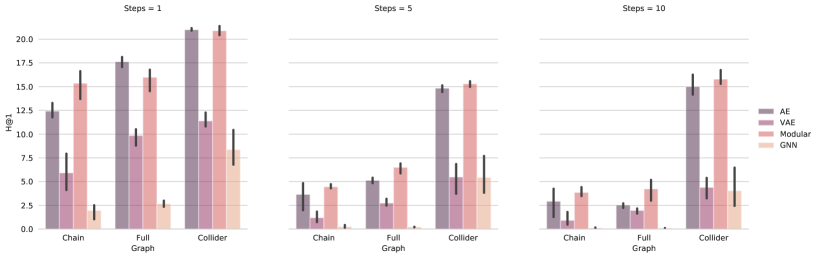
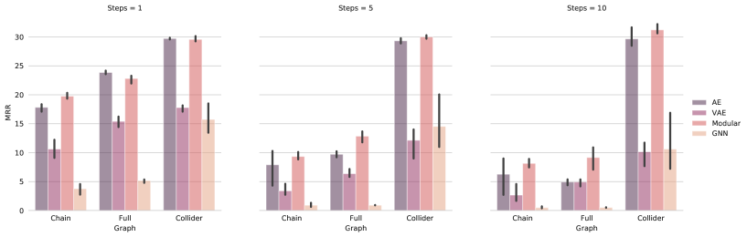
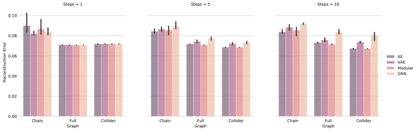
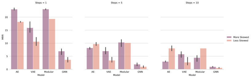
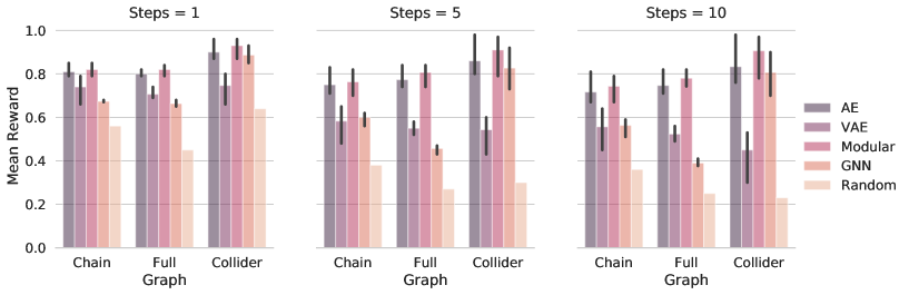
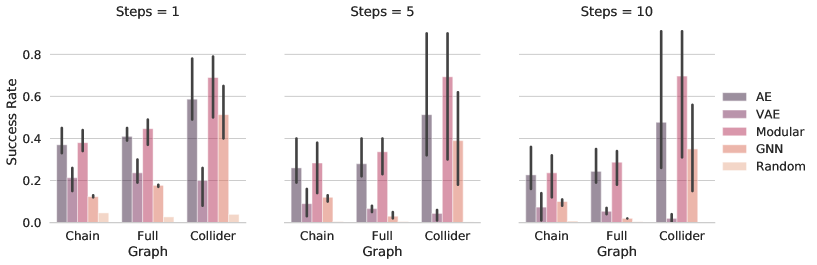
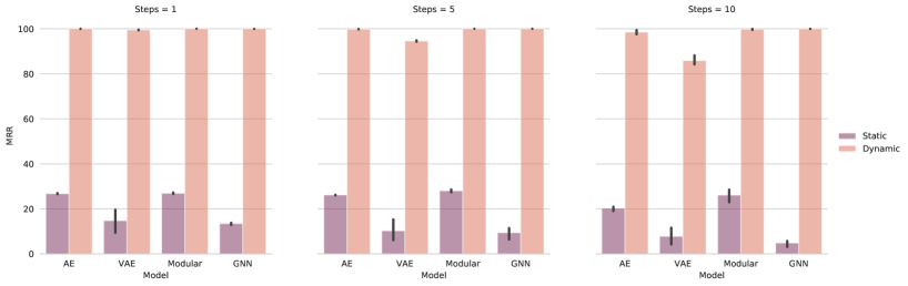
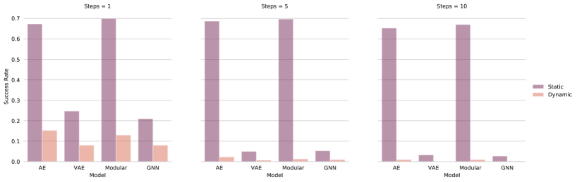
		1 Step			5 Steps			10 Steps
Graph Type	Model	H@1	MRR	Rec.	H@1	MRR	Rec.	H@1	MRR	Rec.
Chain NLL	AE	16.937_{$\pm$ 0.386}	23.007_{$\pm$ 0.133}	0.07_{$\pm$ 0.0}	4.433_{$\pm$ 0.023}	8.187_{$\pm$ 0.118}	0.073_{$\pm$ 0.0}	1.48_{$\pm$ 0.04}	2.957_{$\pm$ 0.063}	0.076_{$\pm$ 0.0}
	VAE	10.293_{$\pm$ 2.711}	15.897_{$\pm$ 2.927}	0.071_{$\pm$ 0.0}	2.987_{$\pm$ 0.282}	6.983_{$\pm$ 1.079}	0.075_{$\pm$ 0.0}	2.19_{$\pm$ 0.184}	5.78_{$\pm$ 0.821}	0.076_{$\pm$ 0.0}
	Modular	16.863_{$\pm$ 0.135}	23.047_{$\pm$ 0.027}	0.07_{$\pm$ 0.0}	5.317_{$\pm$ 0.249}	10.31_{$\pm$ 1.343}	0.072_{$\pm$ 0.0}	2.04_{$\pm$ 0.259}	4.45_{$\pm$ 1.043}	0.074_{$\pm$ 0.0}
	GNN	3.587_{$\pm$ 0.412}	6.93_{$\pm$ 0.91}	0.07_{$\pm$ 0.0}	0.617_{$\pm$ 0.05}	1.9_{$\pm$ 0.195}	0.076_{$\pm$ 0.0}	0.257_{$\pm$ 0.002}	0.947_{$\pm$ 0.023}	0.079_{$\pm$ 0.0}
Full NLL	AE	17.62_{$\pm$ 0.192}	23.85_{$\pm$ 0.065}	0.071_{$\pm$ 0.0}	5.127_{$\pm$ 0.058}	9.707_{$\pm$ 0.184}	0.072_{$\pm$ 0.0}	2.527_{$\pm$ 0.045}	4.913_{$\pm$ 0.177}	0.073_{$\pm$ 0.0}
	VAE	9.847_{$\pm$ 0.572}	15.407_{$\pm$ 0.559}	0.071_{$\pm$ 0.0}	2.747_{$\pm$ 0.104}	6.363_{$\pm$ 0.342}	0.074_{$\pm$ 0.0}	1.957_{$\pm$ 0.056}	4.927_{$\pm$ 0.289}	0.076_{$\pm$ 0.0}
	Modular	15.977_{$\pm$ 1.066}	22.813_{$\pm$ 0.374}	0.071_{$\pm$ 0.0}	6.493_{$\pm$ 0.209}	12.837_{$\pm$ 0.62}	0.071_{$\pm$ 0.0}	4.233_{$\pm$ 0.848}	9.157_{$\pm$ 2.529}	0.071_{$\pm$ 0.0}
	GNN	2.68_{$\pm$ 0.073}	5.15_{$\pm$ 0.069}	0.071_{$\pm$ 0.0}	0.23_{$\pm$ 0.001}	0.913_{$\pm$ 0.001}	0.077_{$\pm$ 0.0}	0.103_{$\pm$ 0.001}	0.503_{$\pm$ 0.002}	0.084_{$\pm$ 0.0}
Collider NLL	AE	20.993_{$\pm$ 0.016}	29.723_{$\pm$ 0.014}	0.072_{$\pm$ 0.0}	14.84_{$\pm$ 0.09}	29.32_{$\pm$ 0.135}	0.069_{$\pm$ 0.0}	15.01_{$\pm$ 0.829}	29.657_{$\pm$ 2.029}	0.067_{$\pm$ 0.0}
	VAE	9.847_{$\pm$ 0.572}	15.407_{$\pm$ 0.559}	0.071_{$\pm$ 0.0}	2.747_{$\pm$ 0.104}	6.363_{$\pm$ 0.342}	0.074_{$\pm$ 0.0}	1.957_{$\pm$ 0.056}	4.927_{$\pm$ 0.289}	0.076_{$\pm$ 0.0}
	Modular	20.89_{$\pm$ 0.16}	29.563_{$\pm$ 0.173}	0.072_{$\pm$ 0.0}	15.297_{$\pm$ 0.063}	29.99_{$\pm$ 0.062}	0.068_{$\pm$ 0.0}	15.78_{$\pm$ 0.47}	31.21_{$\pm$ 0.515}	0.067_{$\pm$ 0.0}
	GNN	8.377_{$\pm$ 2.358}	15.737_{$\pm$ 4.398}	0.072_{$\pm$ 0.0}	5.443_{$\pm$ 2.729}	14.527_{$\pm$ 15.714}	0.073_{$\pm$ 0.0}	4.04_{$\pm$ 3.073}	10.607_{$\pm$ 20.141}	0.08_{$\pm$ 0.0}

Table 17: Hits at Rank 1 (H@1), Mean Reciprocal Rank (MRR) (higher is better) and Reconstruction Error (lower is better) for different models trained using NLL loss for 1, 5 and 10 step prediction for the vanilla chemistry environment with 5 objects and 5 colors.

		1 Step		5 Steps		10 Steps
Graph Type	Model	Mean Reward	Success	Mean Reward	Success	Mean Reward	Success
Chain	Random	0.56	0.046	0.38	0.005	0.36 0.007
	Optimal	0.86	0.52	0.83	0.39	0.16	0.38
	AE	0.81_{$\pm$ 0.001}	0.37_{$\pm$ 0.003}	0.75_{$\pm$ 0.003}	0.26_{$\pm$ 0.01}	0.717_{$\pm$ 0.004}	0.227_{$\pm$ 0.009}
	VAE	0.74_{$\pm$ 0.003}	0.213_{$\pm$ 0.002}	0.583_{$\pm$ 0.005}	0.09_{$\pm$ 0.003}	0.557_{$\pm$ 0.006}	0.073_{$\pm$ 0.003}
	Modular	0.82_{$\pm$ 0.001}	0.38_{$\pm$ 0.002}	0.763_{$\pm$ 0.002}	0.283_{$\pm$ 0.011}	0.743_{$\pm$ 0.003}	0.237_{$\pm$ 0.007}
	GNN	0.673_{$\pm$ 0.0}	0.123_{$\pm$ 0.0}	0.6_{$\pm$ 0.001}	0.12_{$\pm$ 0.0}	0.563_{$\pm$ 0.001}	0.1_{$\pm$ 0.0}
Full	Random	0.45	0.027	0.27	0.005	0.25	0.004
	Optimal	0.79	0.44	0.737	0.275	0.72	0.24
	AE	0.8_{$\pm$ 0.0}	0.41_{$\pm$ 0.001}	0.773_{$\pm$ 0.002}	0.28_{$\pm$ 0.007}	0.747_{$\pm$ 0.003}	0.243_{$\pm$ 0.006}
	VAE	0.707_{$\pm$ 0.001}	0.237_{$\pm$ 0.002}	0.55_{$\pm$ 0.001}	0.067_{$\pm$ 0.0}	0.523_{$\pm$ 0.001}	0.053_{$\pm$ 0.0}
	Modular	0.82_{$\pm$ 0.0}	0.447_{$\pm$ 0.003}	0.807_{$\pm$ 0.002}	0.337_{$\pm$ 0.006}	0.78_{$\pm$ 0.002}	0.287_{$\pm$ 0.006}
	GNN	0.663_{$\pm$ 0.0}	0.177_{$\pm$ 0.0}	0.457_{$\pm$ 0.0}	0.03_{$\pm$ 0.0}	0.39_{$\pm$ 0.0}	0.02_{$\pm$ 0.0}
Collider	Random	0.45	0.23	0.27	0.005	0.25	0.004
	Optimal	0.95	0.75	0.94	0.733	0.96	0.80
	AE	0.9_{$\pm$ 0.002}	0.587_{$\pm$ 0.019}	0.86_{$\pm$ 0.007}	0.513_{$\pm$ 0.075}	0.833_{$\pm$ 0.011}	0.477_{$\pm$ 0.094}
	VAE	0.747_{$\pm$ 0.004}	0.2_{$\pm$ 0.007}	0.543_{$\pm$ 0.006}	0.043_{$\pm$ 0.001}	0.45_{$\pm$ 0.011}	0.02_{$\pm$ 0.0}
	Modular	0.93_{$\pm$ 0.002}	0.69_{$\pm$ 0.018}	0.91_{$\pm$ 0.007}	0.693_{$\pm$ 0.077}	0.907_{$\pm$ 0.008}	0.697_{$\pm$ 0.075}
	GNN	0.887_{$\pm$ 0.001}	0.513_{$\pm$ 0.011}	0.827_{$\pm$ 0.006}	0.39_{$\pm$ 0.032}	0.807_{$\pm$ 0.007}	0.35_{$\pm$ 0.028}

Table 18: Mean reward and Success rate (higher is better) for 1, 5 and 10 step for the vanilla setting of the chemistry environment with 5 objects and 5 colors. This table uses models trained using NLL loss.