Exploration noise for learning linear-quadratic mean field games

Abstract.

The goal of this paper is to demonstrate that common noise may serve as an exploration noise for learning the solution of a mean field game. This concept is here exemplified through a toy linear-quadratic model, for which a suitable form of common noise has already been proven to restore existence and uniqueness. We here go one step further and prove that the same form of common noise may force the convergence of the learning algorithm called ‘fictitious play’, and this without any further potential or monotone structure. Several numerical examples are provided in order to support our theoretical analysis.

1. Introduction

1.1. General context.

Since their inception fifteen years ago in the seminal works of Lasry and Lions [55, 56, 57], Lions [58] and Huang et al. [49, 51, 50], mean field games (MFGs) have met a tremendous success, inspiring mathematical works from different areas like partial differential equations (PDEs), control theory, stochastic analysis, calculus of variation, toward a consistent and expanded theory for games with many weakly interacting rational agents. Meanwhile, the increasing number of applications has stimulated a long series of works on discretization and numerical methods for approximating the underlying equilibria (which we also call solutions); see for instance Achdou et al. [1, 2], Achdou and Capuzzo-Dolcetta [3] and Achdou and Laurière [4] for discretization with finite differences; Carlini and Silva [15, 16] for semi-Lagrangian schemes; Benamou and Carlier [9] and Bricenõ Arias et al. [13, 12] for variational discretization; and Achdou and Laurière [5] for an overview. These contributions often include numerical methods for solving the discrete schemes such as the Picard method, Newton method, fictitious play. We review the latter one in detail in the sequel. Recently, other works have also demonstrated the possible efficiency of tools from machine learning within this complex framework: standard equations for characterizing the equilibria may be approximately solved by means of a neural network; see for instance Carmona and Laurière [20, 23]. Last (but not least), motivated by the desire to develop methods for models with partially unknown data, several authors have integrated important concepts from reinforcement learning in their studies; we refer to Carmona et al. [21, 22], Elie et al. [38] and Guo et al. [43].

The aim of our work is to make one new step forward in the latter direction with a study at the frontier between the theoretical analysis of MFGs and the development of appropriate forms of learning. In particular, our main objective is to provide a proof of concept for the notion of exploration noise, which is certainly a key ingredient in machine learning. For the reader who is aware of the MFG theory, our basic idea is to prove that common noise may indeed serve for the exploration of the space of solutions and, in the end, for the improvement of the existing learning algorithms. For sure, this looks a very ambitious program since there has not been, so far, any complete understanding of the impact of the common noise onto the shape of the solutions. However, several recent works clearly indicate that noise might be helpful for numerical purposes. Indeed, in a series of works, Bayraktar et al. [7], Delarue [31], and Foguen Tchuendom [40], it was shown that common noise could help to force uniqueness of equilibria in a certain number of MFGs. This is a striking fact because nonuniqueness is the typical rule for MFGs, except in some particular classes with some specific structure; see for instance the famous uniqueness result of Lasry and Lions [55] for games with monotonous coefficients and Carmona and Delarue [17, chapter 3]. Conceptually, the key condition for forcing uniqueness is that, under the action of the (hence common) noise, the equilibria can visit sufficiently well the state space in which they live. This makes the whole rather subtle because, in full theory, the state space is the space of probability measures, which is typically infinite-dimensional. In this respect, the main examples for which such a smoothing effect has been rigorously established so far are $(i)$ a linear quadratic model with possibly nonlinear mean field interaction terms in the cost functional (Foguen Tchuendom [40]), $(ii)$ a general model with an infinite dimensional noise combined with a suitable form of local interaction in the dynamics (Delarue [31]); and $(iii)$ models defined on finite state spaces and forced by a variant of the Wright-Fisher noise used in population genetics literature (Bayraktar et al. [7]).

In order to prove the possible efficiency of our approach, we here restrict the whole discussion to the first of the three aforementioned instances. We provide below a long informative introduction in which we present the model in detail together with the related literature and our own results. The guideline of this introduction is the following. We specify the model in Subsection 1.2, both without and with common noise. In particular, we recall therein the various known characterizations of the equilibria in both cases. In Subsection 1.3, we provide a brief review of the existing learning procedures and we exemplify the form of the so-called fictitious play for the linear-quadratic model studied in the paper. The thrust of our paper is to introduce a variant of the fictitious play, which we refer to as the tilted fictitious play and whose convergence can be proven in the presence of common noise under more general conditions than those of the standard fictitious play (within the class of linear-quadratic MFGs introduced in Subsection 1.2). This tilted fictitious play is defined in Subsection 1.4. Although the tilted fictitious play can be regarded as a theoretical learning scheme, we explain in Subsection 1.5 how it can be adapted to statistical learning. Notably, in this adaptation, the common noise serves as an exploration noise for learning the equilibria of the underlying MFG. This interpretation of the common noise in terms of exploration is in fact one key point of the paper. Exploitation is then briefly addressed in Subsection 1.6. Therein, we present the main bounds that we are able to prove for the mean exploitability of the policy that is returned by the tilted fictitious play. Finally, we provide an overview of our numerical results in Subsection 1.7, and we conclude the introduction by providing a comparison with the existing literature in Subsection 1.8. The main assumption and notation are given in Subsection 1.9. The organization of the paper is also presented in Subsection 1.9.

1.2. Our model.

In this subsection, we expose the linear-quadratic class of MFGs that is addressed in the paper, without and with common noise. We insist in both cases on the form of the equilibrium feedbacks. As made clear in (1.5), those feedbacks are necessarily affine. Moreover, for any of them, the intercept in the affine structure is characterized by a backward stochastic differential equation (BSDE), which is recalled in (1.6) and which plays a key role in the subsequent analysis.

To make it clear, the MFG that we consider below comprises the state equation

$$\mathrm{d}X_{t}=\alpha_{t}\mathrm{d}t+\sigma\mathrm{d}B_{t}+\varepsilon\mathrm{d}W_{t},\quad t\in[0,T],$$ (1.1)

together with the cost functional

$$J\bigl{(}{\bm{\alpha}};{\bm{m}}\bigr{)}=\frac{1}{2}{\mathbb{E}}\biggl{[}\bigl{|}RX_{T}+g(m_{T})\bigr{|}^{2}+\int_{0}^{T}\Bigl{\{}\bigl{|}QX_{t}+f(m_{t})\bigr{|}^{2}+|\alpha_{t}|^{2}\Bigr{\}}\mathrm{d}t\biggr{]}.$$ (1.2)

Above, $X_{t}$ is the state at time $t$ of a representative agent evolving within a continuum of other agents. It takes values in ${\mathbb{R}}^{d}$, for some integer $d\geq 1$, and evolves from the initial time $0$ to the terminal time $T$ according to the equation (1.1). Therein, ${\bm{B}}=(B_{t})_{0\leq t\leq T}$ and ${\bm{W}}=(W_{t})_{0\leq t\leq T}$ are two independent $d$-dimensional Brownian motions on a complete probability space $(\Omega,{\mathcal{A}},{\mathbb{P}})$, and $\sigma\geq 0$ and $\varepsilon\geq 0$ account for their respective intensity in the dynamics. Whereas ${\bm{B}}$ is thought as a private (or idiosyncratic) noise felt by the representative player only (and not by the others), the process ${\bm{W}}$ is said to be a common or systemic noise as all the others in the continuum also feel it. The initial condition (also called initial private state) $X_{0}$ may be random and, in any case, $X_{0}$ is independent of the pair $({\bm{B}},{\bm{W}})$. The process ${\bm{\alpha}}=(\alpha_{t})_{0\leq t\leq T}$ is a so-called control process, which is usually assumed to be progressively-measurable with respect to the augmented filtration ${\mathbb{F}}$ generated by $(X_{0},\sigma{\bm{B}},\varepsilon{\bm{W}})$ (when $\sigma$ or $\varepsilon$ are zero, the corresponding process is no longer used to generate the filtration). The key fact in MFG theory is that the representative player aims at choosing the best possible ${\bm{\alpha}}$ in order to minimize the cost functional $J$ in (1.2). The leading symbol ${\mathbb{E}}$ in the definition of $J$ is understood as an expectation with respect to all the inputs $(X_{0},{\bm{B}},{\bm{W}})$. If there were no dependence on the extra term ${\bm{m}}=(m_{t})_{0\leq t\leq T}$ in $f$ and $g$, the minimization of $J$ would reduce to a mere linear-quadratic stochastic control problem driven by $Q$ and $R$, with the latter being two $d$-square matrices. The essence of MFGs is that $(m_{t})_{0\leq t\leq T}$ accounts for the flow of marginal statistical states of the continuum of players surrounding the representative agent. In full generality, each $m_{t}$ should be regarded as a probability measure hence describing the statistical distribution of the other agents at time $t$. For simplicity, we here just assume $m_{t}$ to be the $d$-dimensional mean of the other agents at time $t$; consistently, $f=(f^{1},\cdots,f^{d})$ and $g=(g^{1},\cdots,g^{d})$ are ${\mathbb{R}}^{d}$-valued functions defined on ${\mathbb{R}}^{d}$. However, the notion of mean should be clarified, because of the distinction between the two private and common noises. From a modelling point of view, this mean should result from a law of large numbers taken over players that would be subjected to independent and identically distributed (i.i.d.) initial and private noises (consistently with our former description of ${\bm{B}}$) but to the same common noise ${\bm{W}}$. Because of this, $(m_{t})_{0\leq t\leq T}$ is itself required to be a stochastic process, progressively-measurable with respect to the filtration generated by $\varepsilon{\bm{W}}$. When $\varepsilon=0$, the filtration becomes trivial and, accordingly, $(m_{t})_{0\leq t\leq T}$ is assumed to be deterministic. The notion of Nash equilibrium or MFG solution then comes through a fixed point argument. In short, $(m_{t})_{0\leq t\leq T}$ is said to be an equilibrium if the minimizer $(X_{t}^{\star})_{0\leq t\leq T}$ of (1.1)–(1.2) satisfies:

$$m_{t}={\mathbb{E}}\bigl{[}X_{t}^{\star}\,|\,\varepsilon{\bm{W}}\bigr{]},\quad t\in[0,T],$$ (1.3)

with the conditional expectation becoming an expectation if $\varepsilon=0$ (whence our choice to use $\varepsilon{\bm{W}}$ as random variable in the conditioning, as this notation allows us to distinguish easily between the two cases without and with common noise). Throughout, $f$ and $g$ are typically assumed to be bounded and Lipschitz continuous functions. When $\varepsilon=0$, this is enough for ensuring the existence of solutions to the fixed point (1.3), but uniqueness is known to fail in general, except under some additional conditions. For instance, the Lasry-Lions monotonicity condition, when adapted to this setting, says that uniqueness indeed holds true if $Q^{\dagger}f$ and $R^{\dagger}g$ (with $\dagger$ denoting the transpose) are non-decreasing in the sense that (see [32])

$$\forall x,x^{\prime}\in{\mathbb{R}}^{d},\quad(x-x^{\prime})\cdot\bigl{(}Q^{\dagger}f(x)-Q^{\dagger}f(x^{\prime})\bigr{)}\geq 0,\quad(x-x^{\prime})\cdot\bigl{(}R^{\dagger}g(x)-R^{\dagger}g(x^{\prime})\bigr{)}\geq 0,$$ (1.4)

with $\cdot$ denoting the standard inner product in ${\mathbb{R}}^{d}$. When $\varepsilon>0$, existence and uniqueness hold true, even though the coefficients are not monotone (see [40]). This is a very clear instance of the effective impact of the noise onto the search of equilibria.

The reason why the MFG (1.1)–(1.2)–(1.3) becomes uniquely solvable under the action of the common noise may be explained as follows. In short (and this is the rationale for working in this set-up), the linear-quadratic structure of (1.1) forces uniqueness of the minimizer to (1.2) when ${\bm{m}}$ is fixed. Even more the optimal control is given in the Markovian form

$$\alpha_{t}^{\star}=-\eta_{t}X_{t}^{\star}-h_{t},\quad t\in[0,T],$$ (1.5)

where ${\bm{\eta}}=(\eta_{t})_{0\leq t\leq T}$ is the $d\times d$-matrix valued solution of an autonomous Riccati equation that only depends on $Q$ and $R$ and that is in particular independent of the input ${\bm{m}}$. In other words, only the intercept $({\bm{h}}_{t})_{0\leq t\leq T}$ in the above formula depends on the inputs $f$, $g$, $R$, $Q$ and ${\bm{m}}$. The characterization of ${\bm{h}}$ is usually obtained by the (stochastic if $\varepsilon>0$) Pontryagin principle, namely ${\bm{h}}$ solves the Backward Stochastic Differential Equation (BSDE)

$$h_{t}=R^{\dagger}g(m_{T})+\int_{t}^{T}\bigl{\{}Q^{\dagger}f(m_{s})-\eta_{s}h_{s}\bigr{\}}\mathrm{d}s-\varepsilon\int_{t}^{T}k_{s}\mathrm{d}W_{s},\quad t\in[0,T].$$ (1.6)

When $\varepsilon=0$, the above stochastic integral disappears and the equation (1.6) becomes a mere Ordinary Differential Equation (ODE) but set backwards in time. When $\varepsilon>0$, the solution is the pair $({\bm{h}},{\bm{k}})$, which is required to be progressively measurable with respect to the filtration generated by ${\bm{W}}$. Existence and uniqueness are well-known facts in BSDE theory. By taking the conditional mean given ${\bm{W}}$ in (1.1), we deduce that solving the MFG problem thus amounts to find a pair $({\bm{m}},{\bm{h}})$ satisfying the forward-backward stochastic differential equation (FBSDE):

$$\begin{split}&\mathrm{d}m_{t}=-\bigl{(}\eta_{t}m_{t}+h_{t}\bigr{)}\mathrm{d}t+\varepsilon\mathrm{d}W_{t},\quad m_{0}={\mathbb{E}}(X_{0}),\\ &\mathrm{d}h_{t}=-\bigl{(}Q^{\dagger}f(m_{t})-\eta_{t}h_{t}\bigr{)}\mathrm{d}t+\varepsilon k_{t}\mathrm{d}W_{t},\quad h_{T}=R^{\dagger}g(m_{T}).\end{split}$$ (1.7)

Unique solvability was proven in [29, 59]. The smoothing effect of the noise manifests at the level of the related system of Partial Differential Equations (PDEs), which is sometimes called the master equation of the game:

$$\partial_{t}\theta_{\varepsilon}(t,x)+\tfrac{\varepsilon^{2}}{2}\Delta^{2}_{xx}\theta_{\varepsilon}(t,x)-\bigl{(}\eta_{t}x+\theta_{\varepsilon}(t,x)\bigr{)}\cdot\nabla_{x}\theta_{\varepsilon}(t,x)+Q^{\dagger}f(x)-\eta_{t}\theta_{\varepsilon}(t,x)=0,$$ (1.8)

with $\theta_{\varepsilon}(T,\cdot)=R^{\dagger}g(\cdot)$ as a boundary condition at the terminal time, $\theta_{\varepsilon}$ being a function from $[0,T]\times{\mathbb{R}}^{d}\rightarrow{\mathbb{R}}^{d}$. When $\varepsilon>0$, the PDE is uniformly parabolic and hence has a unique classical solution (with bounded derivatives). When $\varepsilon=0$, it becomes an hyperbolic equation and singularities may emerge, precisely when the solutions to (1.7) (which are nothing but the characteristics of (1.8)) cease to be unique.

1.3. Learning procedures

We now provide an overview of the existing methods that can be used for solving the standing MFG numerically, or at least for decoupling the two forward and backward equations in (1.7). In particular, we spend some time here recalling the definition of the so-called fictitious play, see (1.9) and (1.10).

In our setting, numerical solutions to the MFG may be found by solving either the FBSDE (1.7) or the nonlinear equation (1.8). For sure, independently of any applications to MFGs, there have been well-known numerical methods for the two objects, see for instance (and for a tiny example) Beck et al. [8], Bender and Zhang [10], Cvitanić and Zhang [28], Delarue and Menozzi [33], E et al. [37], Huijskens et al. [52], Ma et al. [60], and Milstein and Tretyakov [61]. In Delarue and Menozzi [33], Huijskens et al. [52], Ma et al. [60], and Milstein and Tretyakov [61], the problem is solved by constructing an approximation of $\theta_{\varepsilon}$ by means of a backward induction. This is a typical strategy in the field, which is fully consistent with the dynamic programming principle that holds true for uniquely solvable mean field games (see [18, chapter 4]). Although formulated differently, Bender and Zhang [10] also relies on a backward induction. In comparison with Bender and Zhang [10], Delarue and Menozzi [33], Huijskens et al. [52], Ma et al. [60], and Milstein and Tretyakov [61], the works Beck et al. [8], Cvitanić and Zhang [28], and E et al. [37] proceed in a completely different manner because the backward equation therein is reformulated into a forward equation with an unknown initial condition; the goal is then to tune both the initial condition and the martingale representation term of the backward equation in order to minimize, at terminal time, the distance to the prescribed boundary condition. Those methods have the following main limitation within a learning prospect for MFGs: they require the coefficients $f$, $g$, $Q$ and $R$ entering the model to be explicitly known. Even more, they make no real use of the control structure (1.2) that underpins the game.

In fact, Delarue and Menozzi [33], Huijskens et al. [52], Ma et al. [60], and Milstein and Tretyakov [61] suffer from another drawback because all these works involve a space discretization that consists in approximating the function $\theta_{\varepsilon}$ at the nodes of a spatial grid. Accordingly, the complexity increases with the physical dimension $d$ of the state variable. In particular, similar strategies would become even more costly for a more general mean field dependence than the one addressed in (1.2). Indeed, in the general case, the spatial variable is no longer the mean but the whole statistical distribution (which is an infinite dimensional object). For sure, the latter raises challenging questions that go beyond the scope of this paper because we cannot guess of a numerical method that would directly allow to handle the infinite dimensional statistical distribution of the solution. However, this is an objective that should be kept in mind. Say for instance that particle or quantization methods would be natural candidates to overcome such an issue, see for instance Chaudru de Raynal and Garcia Trillos [26] and Crisan and McMurray [27].

Whatever the method, the true difficulty is to decouple (1.7), because the two forward and backward time directions are conflicting. One of our basic concern here is thus to take benefit of the noise in order to define an iterative scheme that decouples (1.7) efficiently. At the same time, because the very structure of a MFG corresponds very naturally to the precepts of reinforcement learning, we want to have a method that may work with unknown coefficients $f$, $g$, $Q$ and $R$, and that may benefit from the observation of the cost if it is available. In this regard, we ask our scheme to have a learning structure that should manifest in a sequence of steps of the form

1. computation of a best action,

2. update of the state variable,

and hence that would be adapted to real data. Surprisingly, this is not an easy question, even though the equation (1.7) is well-posed. As demonstrated in the recent work [25], naive Picard iterations may indeed fail. They would consist in solving inductively the backward equation

$$\mathrm{d}h_{t}^{n+1}=-\bigl{(}Q^{\dagger}f(\overline{m}_{t}^{n})-\eta_{t}h_{t}^{n+1}\bigr{)}\mathrm{d}t+\varepsilon k_{t}^{n+1}\mathrm{d}W_{t},\quad h_{T}^{n+1}=R^{\dagger}g(\overline{m}_{T}^{n}).$$ (1.9)

for a given proxy $\overline{\bm{m}}^{n}:=(\overline{m}_{t}^{n})_{0\leq t\leq T}$ of the forward equation and then in plugging the solution ${\bm{h}}^{n+1}:=(h_{t}^{n+1})_{0\leq t\leq T}$ into the forward equation

$$\mathrm{d}\overline{m}_{t}^{n+1}=-\bigl{(}\eta_{t}\overline{m}_{t}^{n+1}+h_{t}^{n+1}\bigr{)}\mathrm{d}t+\varepsilon\mathrm{d}W_{t},\quad m_{0}^{n+1}={\mathbb{E}}(X_{0}).$$ (1.10)

Intuitively, the reason why it may fail is that the updating rule $\overline{\bm{m}}^{n}\mapsto\overline{\bm{m}}^{n+1}$ is too ambitious. In other words, the increment may be too high and smaller steps are needed to guarantee the convergence of the procedure.

A more successful strategy is known in MFG theory (and more generally in game theory) under the name of fictitious play, see [14, 38, 41, 44, 45, 65, 66]. It is a learning procedure with a decreasing harmonic step of size $1/n$ at rank $n$ of the iteration. Having as before a proxy $\overline{\bm{m}}^{n}$ for the state of the population at rank $n$ of the learning procedure, ${\bm{h}}^{n+1}$ is computed as above. Next, the same forward equation as before is also solved, but the solution is denoted by ${\bm{m}}^{n+1}$, namely

$$\mathrm{d}{m}_{t}^{n+1}=-\bigl{(}\eta_{t}m_{t}^{n+1}+h_{t}^{n}\bigr{)}\mathrm{d}t+\varepsilon\mathrm{d}W_{t},\quad m_{0}^{n+1}={\mathbb{E}}(X_{0}),$$ (1.11)

and then the updating rule is given by

$$\overline{m}_{t}^{n+1}=\frac{1}{n+1}m_{t}^{n+1}+\frac{n}{n+1}\overline{m}_{t}^{n},\quad t\in[0,T].$$ (1.12)

Very importantly, both the Picard iteration and the fictitious play have a learning interpretation. In both cases, the backward equation (1.9) provides the best response ${\bm{\alpha}}^{n+1,\star}$ to the minimization of the functional ${\bm{\alpha}}\mapsto J({\bm{\alpha}};\overline{\bm{m}}^{n})$, which has indeed the same form as in (1.5):

$$\alpha_{t}^{n+1}=-\eta_{t}X_{t}^{n+1}-h_{t}^{n+1},\quad t\in[0,T],$$

where $(X_{t}^{n+1,\star})_{0\leq t\leq T}$ is obtained implicitly by solving the corresponding state equation (1.1). Equivalently, the above formula gives the form of the optimal feedback function to the minimization of the functional ${\bm{\alpha}}\mapsto J({\bm{\alpha}};\overline{\bm{m}}^{n})$ (bearing in mind that the feedback function may be here random because of the common noise).

In fact, the fictitious play has been addressed so far in the following two main cases: potential MFGs ([14]) and MFGs with monotone coefficients (here, $Q^{\dagger}f$ and $R^{\dagger}g$ are non-decreasing; see [38, 41, 44, 45, 66] within a general setting). Also, except in the recent work [66] (whose framework is a bit different because the fictitious play is in continuous time), the analysis has just been carried out in the case $\varepsilon=0$, i.e., when there is no common noise. Here, it is certainly useful to recall that potential MFGs are a class of MFGs for which there exists a potential, namely a functional ${\mathcal{J}}({\bm{\alpha}})$ associated with the same state dynamics as in (1.1)–(1.2), such that any minimizer of ${\mathcal{J}}$ is a solution of the MFG. In our setting, the shape of ${\mathcal{J}}({\bm{\alpha}})$ is

$${\mathcal{J}}\bigl{(}{\bm{\alpha}}\bigr{)}={\mathbb{E}}\biggl{[}{\mathcal{G}}\bigl{(}{\mathcal{L}}(X_{T}|\varepsilon{\bm{W}})\bigr{)}+\int_{0}^{T}\frac{1}{2}\Bigl{[}{\mathcal{F}}\bigl{(}{\mathcal{L}}(X_{t}|\varepsilon{\bm{W}})\bigr{)}+|\alpha_{t}|^{2}\Bigr{]}\mathrm{d}t\biggr{]},$$ (1.13)

where ${\mathcal{L}}(X_{t}|\varepsilon{\bm{W}})$ denotes the conditional law of $X_{t}$ given the common noise and

$${\mathcal{G}}(\mu)=\frac{1}{2}\int_{{\mathbb{R}}^{d}}|Rx|^{2}\mathrm{d}\mu(x)+G\bigl{(}\bar{\mu}\bigr{)},\quad{\mathcal{F}}(\mu)=\frac{1}{2}\int_{{\mathbb{R}}^{d}}|Qx|^{2}\mathrm{d}\mu(x)+F\bigl{(}\bar{\mu}\bigr{)},$$ (1.14)

with $G$ and $F$ denoting primitives of $R^{\dagger}g$ and $Q^{\dagger}f$ (if any). In particular, the model is always potential when $d=1$, but there is no potential structure when $d\geq 2$, unless $Q^{\dagger}f$ and $R^{\dagger}g$ both derive from (Euclidean) potentials, meaning that $(Q^{\dagger}f)^{i}=\partial F/\partial x_{i}$ and $(R^{\dagger}g)^{i}=\partial G/\partial x_{i}$.

1.4. Tilted harmonic and geometric fictitious plays

This subsection contains one of the main novelties of the paper. For reasons that are explained below, we introduce two variants of the fictitious play, which we call ‘tilted harmonic’ and ‘tilted geometric’. The definition of the geometric version (which is the version that is effectively addressed in the paper) consists of the four equations (1.24)–(1.20)–(1.21)–(1.25) below and differs significantly from (1.11)–(1.12).

Consistently with our agenda, our goal is indeed to prove that the fictitious play may converge thanks to the presence of the common noise (i.e., $\varepsilon>0$). Seemingly, the above discussion about the potential structure of our model in dimension $d=1$ demonstrates that this question becomes especially relevant in dimension greater than or equal to 2 (the results from [14] could be easily adapted to this setting, even in the presence of the common noise). In fact, as shown in Subsection 3.5, the question is also interesting in dimension $d=1$ in cases when equilibria are not unique.

However, this program is more challenging than it seems because we are not able, even in the presence of the common noise, to prove the convergence of the fictitious play stated in (1.9) and (1.11). Instead, we take benefit of the noise in order to reformulate the two equations (1.9) and (1.11) into a new system obtained by a mere shift of the common noise. By Girsanov theorem, the new shifted common noise has the same law as the original one but under a tilted probability measure. Using the harmonic updating rule (1.12), this so-called tilted harmonic scheme is then shown to converge (in the case $\varepsilon>0$).

In order to state the new fictitious play properly, we thus need to allow for another form of common noise in (1.1). For a process ${\bm{h}}=(h_{t})_{0\leq t\leq T}$, progressively-measurable with respect to the filtration generated by ${\bm{W}}$, we thus introduce the shifted Brownian motion

$${\bm{W}}^{\bm{h}/{\varepsilon}}=\biggl{(}W_{t}^{\bm{h}/{\varepsilon}}:=W_{t}+\frac{1}{\varepsilon}\int_{0}^{t}h_{s}\mathrm{d}s\biggr{)}_{0\leq t\leq T},$$

together with the tilted probability measure ${\mathbb{P}}^{\bm{h}}$ whose density with respect to ${\mathbb{P}}$ is

$${\mathcal{E}}\bigl{(}{\tfrac{1}{\varepsilon}}{\bm{h}}\bigr{)}:=\exp\biggl{(}-\frac{1}{\varepsilon}\int_{0}^{T}h_{t}\cdot\mathrm{d}W_{t}-\frac{1}{2\varepsilon^{2}}\int_{0}^{T}|h_{t}|^{2}\mathrm{d}t\biggr{)}.$$ (1.15)

Accordingly, for any two frozen continuous paths ${\bm{n}}:=(n_{t})_{0\leq t\leq T}$ and ${\bm{w}}:=(w_{t})_{0\leq t\leq T}$, we define the non-averaged cost functional

$${\mathcal{R}}^{x_{0}}\bigl{(}{\bm{\alpha}};{\bm{n}};{\color[rgb]{0,0,0}\varepsilon}{\bm{w}}\bigr{)}:=\frac{1}{2}\biggl{[}\bigl{|}{R}x_{T}+g(n_{T})\bigr{|}^{2}+\int_{0}^{T}\Bigl{\{}\bigl{|}{Q}x_{t}+f(n_{t})\bigr{|}^{2}+|\alpha_{t}|^{2}\Bigr{\}}\mathrm{d}t\biggr{]},$$ (1.16)

where

$$x_{t}=x_{0}+\int_{0}^{t}\alpha_{s}\mathrm{d}s+\sigma B_{t}+\varepsilon w_{t},\quad t\in[0,T],$$ (1.17)

the latter being nothing but the integral version of (1.1), when ${\bm{W}}$ is replaced by the frozen trajectory ${\bm{w}}$. Now, when ${\bm{m}}$ and ${\bm{h}}$ are two progressively-measurable processes with respect to the filtration generated by $\varepsilon{\bm{W}}$, we have a look at the new cost functional:

$$J^{{\varepsilon}}({\bm{\alpha}};{\bm{m}};{\bm{h}}):={\mathbb{E}}^{\bm{h}/{\varepsilon}}\Bigl{[}{\mathcal{R}}^{X_{0}}\bigl{(}{\bm{\alpha}};{\bm{m}};{\varepsilon}{\bm{W}}^{\bm{h}/{\varepsilon}}\bigr{)}\Bigr{]}.$$ (1.18)

We now define the first version of our titled fictitious play according to a two step iterative learning procedure, whose description at rank $n$ goes as follows:

Harmonic best action:

For a proxy $\overline{\bm{m}}^{n}:=(\overline{m}_{t}^{n})_{0\leq t\leq T}$ of the conditional mean ${\bm{m}}=(m_{t})_{0\leq t\leq T}$ of the in-equilibrium population (as given by the forward component of (1.7)) and a proxy ${\bm{h}}^{n}=(h_{t}^{n})_{0\leq t\leq T}$ of the opposite of the ${\mathbb{F}}^{{\bm{W}}}$-adapted intercept of the equilibrium feedback in (1.5) (as given by the backward component of (1.7)), solve

$${\bm{\alpha}}^{n+1}=\textrm{\rm argmin}_{\bm{\alpha}}{\mathbb{E}}^{{\bm{h}}^{n}{/\varepsilon}}\bigl{[}{\mathcal{R}}^{X_{0}}\bigl{(}{\bm{\alpha}};\overline{\bm{m}}^{n};{\color[rgb]{0,0,0}\varepsilon}{\bm{W}}^{{\bm{h}}^{n}/\varepsilon}\bigr{)}\bigr{]},$$ (1.19)

the infimum being taken over all ${\mathbb{F}}$-progressively measurable (${\mathbb{R}}^{d}$-valued) controls ${\bm{\alpha}}$.

The optimal feedback being of the same linear form as in (1.5) (the proof is given below), we may call ${\bm{h}}^{n+1}=(h^{n+1}_{t})_{0\leq t\leq T}$ the opposite of the resulting intercept.

Harmonic update:

Given ${\bm{h}}^{n+1}$, the optimal trajectory of the above minimization problem is

$$X_{t}^{n+1}=X_{0}-\int_{0}^{t}\bigl{(}\eta_{s}X_{s}^{n+1}+h_{s}^{n+1}\bigr{)}\mathrm{d}s+\sigma B_{t}+\varepsilon W_{t}^{{\bm{h}}^{n}/\varepsilon},\quad t\in[0,T].$$ (1.20)

We then let

$$m^{n+1}_{t}={\mathbb{E}}\bigl{[}X_{t}^{n+1}\,|\,{\bm{W}}\bigr{]},\quad t\in[0,T],$$ (1.21)

together with

$$\overline{m}^{n+1}_{t}=\frac{1}{n+1}\sum_{k=1}^{n+1}m_{t}^{k}=\tfrac{1}{n+1}m_{t}^{n+1}+\tfrac{n}{n+1}\overline{m}^{n}_{t},\quad t\in[0,T].$$ (1.22)

For sure the rationale behind this strategy relies on Girsanov’s transformation. Under the tilted probability measure ${\mathbb{P}}^{{\bm{h}}/\varepsilon}$, the process ${\bm{W}}^{{\bm{h}}/\varepsilon}$ is a new Brownian motion, with the same law as the original (or historical) common noise under ${\mathbb{P}}$. However, the main trick here is to dynamically change the form of the common noise (dynamically with respect to the rank of the iteration in the fictitious play). Precisely, this permits to decouple the two forward and backward equations, as clearly shown if we write the equation for $\overline{\bm{m}}^{n+1}$ as an equation with respect to the historical common noise (the proof is given in (2.6) below):

$$\overline{m}_{t}^{n+1}=m_{0}-\int_{0}^{t}\Bigl{(}\eta_{s}m_{s}^{n+1}+\tfrac{1}{n+1}\bigl{[}h_{s}^{n+1}-h_{s}^{0}\bigr{]}\Bigr{)}\mathrm{d}s+\varepsilon W_{t},\quad t\in[0,T].$$ (1.23)

The forward equation then becomes asymptotically autonomous provided that ${\bm{h}}^{n+1}$ can be bounded independently of $n$, which we succeed to prove in Section 2. In turn, the scheme can be easily shown to converge (notice however that we are not able to prove the convergence of the standard non-tilted fictitious play outside any further potential or monotonicity assumption, even in the presence of the common noise). Moreover, the rate can be proved to decay (at least) like ${\mathcal{O}}(1/n)$, with ${\mathcal{O}}(\cdot)$ standing for the ‘big ${\mathcal{O}}$ Landau notation’. Unfortunately, the best estimate we have for the constant driving the term ${\mathcal{O}}(1/n)$ blows up exponentially fast with $1/\varepsilon^{2}$. Although the numerical experiments that are reported below indicate that the rate may decrease faster than $1/n$ and grow slower than $\exp({\mathcal{O}}(1/\varepsilon^{2}))$, the theoretical guarantee that is hence available for the version of the fictitious play comprising the four equations (1.19)–(1.20)–(1.21)–(1.22) is thus rather poor when the viscosity parameter $\varepsilon$ tends to $0$. This prompts us to provide a variant of the scheme, with an updating step (in equation (1.21)) that is different from $1/(n+1)$ and that yields a more favourable trade-off between $n$ and $\varepsilon^{-2}$ (or equivalently that allows for a cheaper choice of $n$ when $\varepsilon$ is small). In order to clarify things, we refer below to the scheme (1.19)–(1.20)–(1.21)–(1.22) as the ‘tilted harmonic fictitious play’.

In a nutshell, the key point is to perform the following modifications in each of the two steps of the fictitious play, with the new version being called ‘geometric’ for reasons that become obvious in the next few lines:

Geometric best action:

With the same notation as before, use $\varpi X_{0}$ as initial private state, $\varpi{\bm{\alpha}}$ as control, and ${\mathbb{P}}^{\varpi{\bm{h}}^{n}/\varepsilon}$ and ${\bm{W}}^{\varpi{\bm{h}}^{n}/\varepsilon}$ as tilted probability measure and tilted noise, where the rate $\varpi$ is a fixed real that is typically chosen in the interval $(1,\sqrt{2}]$. In words, replace (1.19) by

$${\bm{\alpha}}^{n+1}=\textrm{\rm argmin}_{\bm{\alpha}}{\mathbb{E}}^{{\varpi\bm{h}}^{n}{/\varepsilon}}\bigl{[}{\mathcal{R}}^{\varpi X_{0}}\bigl{(}\varpi{\bm{\alpha}};\overline{\bm{m}}^{n};{\color[rgb]{0,0,0}\varpi}{\varepsilon}{\bm{W}}^{\varpi{\bm{h}}^{n}/\varepsilon}\bigr{)}\bigr{]}.$$ (1.24)

Geometric update:

Accordingly, in (1.20), replace $\varepsilon W_{t}^{{\bm{h}}^{n}/\varepsilon}$ by $\varepsilon W_{t}^{\varpi{\bm{h}}^{n}/\varepsilon}$, and next use the updating formula:

$$\overline{m}^{n+1}_{t}=\frac{\varpi(1-\varpi^{-1})}{1-\varpi^{-(n+1)}}\sum_{k=1}^{n+1}\varpi^{-k}m_{t}^{k}=\tfrac{\varpi^{-n}(1-\varpi^{-1})}{1-\varpi^{-(n+1)}}m^{n+1}_{t}+\Bigl{(}1-\tfrac{\varpi^{-n}(1-\varpi^{-1})}{1-\varpi^{-(n+1)}}\Bigr{)}\overline{m}^{n}_{t},$$ (1.25)

for $t\in[0,T]$.

Here is the main idea. In comparison with (1.20), the optimal trajectory of (1.24) is

$$X_{t}^{n+1}=X_{0}-\int_{0}^{t}\bigl{(}\eta_{s}X_{s}^{n+1}+h_{s}^{n+1}\bigr{)}\mathrm{d}s+\tfrac{1}{\varpi}\sigma B_{t}+\varepsilon W_{t}^{\varpi{\bm{h}}^{n}/\varepsilon},\quad t\in[0,T].$$ (1.26)

The above differs from (1.20) because the intensity of the idiosyncratic noise is $\sigma/\varpi$. Fortunately, this term disappears when taking conditional expectations given the common noise, as done in the formula (1.21). (In fact, one can also recover $\sigma$ as intensity by considering $\varpi{\bm{X}}^{n+1}$ as optimal trajectory, but with $\varpi X_{0}$ as initial condition.) Moreover, it must be stressed that the common noise right above is $\varepsilon{\bm{W}}^{\varpi{\bm{h}}^{n}/\varepsilon}$, whereas it is $\varepsilon{\bm{W}}^{{\bm{h}}^{n}/\varepsilon}$ in (1.20). This says that, under the historical probability measure ${\mathbb{P}}$, (1.26) rewrites

$$X_{t}^{n+1}=X_{0}-\int_{0}^{t}\bigl{(}\eta_{s}X_{s}^{n+1}+h_{s}^{n+1}-\varpi h_{s}^{n}\bigr{)}\mathrm{d}s+\tfrac{1}{\varpi}\sigma B_{t}+\varepsilon W_{t},\quad t\in[0,T].$$ (1.27)

The presence of the factor $\varpi$ in the last term of the drift makes it possible to use the geometric updating formula (1.25). In particular, this is our result to show (see §2.1.2 below) that, under the initialization ${\bm{h}}^{0}=0$, (1.23) becomes

$$\overline{m}_{t}^{n+1}=m_{0}-\int_{0}^{t}\Bigl{(}\eta_{s}m_{s}^{n+1}+\tfrac{(1-\varpi)\varpi^{-n}}{1-\varpi^{-(n+1)}}h^{n+1}_{s}\Bigr{)}\mathrm{d}s+\varepsilon W_{t},\quad t\in[0,T].$$ (1.28)

The reader may easily compare with (1.23). Whereas the difference (with a standard decoupled Ornstein-Uhlenbeck process) decreases like ${\mathcal{O}}(1/n)$ in (1.23), it decreases like ${\mathcal{O}}(\varpi^{-n})$ in (1.28). In the end, this gives a geometric rate of convergence (in the parameter $n$). Although this does not change the presence of a leading constant of size $\exp({\mathcal{O}}(1/\varepsilon^{2}))$, this makes it possible, in order to reach a given theoretical guarantee, to choose a value of $n$ (much) lower than in the tilted harmonic fictitious play. Our main statement in this regard is Theorem 2.4. Also, it is worth adding that, under the obvious convention that

$$\frac{(1-\varpi^{-1})\varpi^{-n}}{1-\varpi^{-(n+1)}}=\frac{1}{n+1}$$ (1.29)

when $\varpi=1$, the updating rule (1.22) coincides with (1.25). For this reason, we sometimes speak about the harmonic scheme (1.19)–(1.20)–(1.21)–(1.22) as a particular case of the geometric scheme when $\varpi=1$. (Notice however that, although it could be easily adapted to the case $\varpi=1$, see Remark 2.6, the statement of Theorem 2.4 does not formally apply to $\varpi=1$ and even if it did, the statement would be in fact trivial.) Last but not least, we stress that, in the definition of the geometric best action, the tilted noise is biased, with $\varpi-1$ as bias. This is an important feature of the scheme and this is the reason why we feel important to distinguish the best action (1.24) from the best action (1.19) and to call the former ‘geometric’ and the second ‘harmonic’.

For sure, the reader may want to reformulate the tilted fictitious play for a more general MFG, with a structure that would no longer be linear-quadratic. Whereas the theory of MFG with an additive finite-dimensional common noise (such as ${\bm{W}}=(W_{t})_{0\leq t\leq T}$) is by now well-established (see for instance the book Carmona and Delarue [18]), the real interest for addressing the same tilted form of the fictitious play but in a wider setting is however not clear to us. Indeed, aforementioned known theoretical results on the smoothing effect of the common noise (see Delarue [31]) require in general an infinite dimensional noise of a much more complicated structure than the additive finite-dimensional noise $(W_{t})_{0\leq t\leq T}$ used in (1.28). For this reason, we have decided to restrict the whole exposition to the linear-quadratic setting, even though (1.24), (1.20), (1.21) and (1.25) could be recast, for the same additive finite-dimensional noise, within a larger framework. Outside the class of linear-quadratic games, the main changes are the following ones. First, the optimal feedback in (1.20) is no longer affine. Second, the mean field fixed point can no longer be formulated in terms of the sole conditional expectation, as it is done in (1.20), but involves the full statistical law of $X^{n+1}_{t}$ given ${\bm{W}}$. Third (and subsequently), the rule (1.25) must be reformulated in terms of the full statistical distributions and not only in terms of their means. We leave the details to the reader. Needless to say, obtaining a relevant extension of the tilted fictitious play for general MFGs remains a very interesting but highly challenging objective.

1.5. Exploration

We now explain how the common noise in the tilted fictitious play can be regarded as an exploration noise for the original MFG without common noise.

For sure, changing the common noise as we have done in the cost functional (1.24) (see also (1.19)) raises indeed many practical questions. In order to understand this properly, we should follow the presentation given in Carmona et al. [21, 22] and think of ${\mathcal{R}}$ as being a black-box representing a decentralized unit. For instance, the box may regulate the consumption/production/storage of energy of a single individual connected to a smart grid, see for instance Alasseur [6] and the references therein; the box may also be an autonomous car moving in a flock of vehicles, see for instance Huang et al. [48].

The black-box operation is described in Figure 1. In this picture, the decentralized black-box receives four inputs: $(i)$ the control, as tuned by the individual operating the black-box; $(ii)$ the initial private state $X_{0}$; $(iii)$ the two idiosyncratic and independent noises; $(iv)$ the state of the population. In this representation, the only input that can be tuned by the individual operating the black-box is the control itself.

Figure 1. Black-box operation for an MFG with a common noise. In the four input arrows, only the plain line can be tuned. Given the input state of the population, the private initial state $X_{0}$ and the realizations of the two noises, the decentralized black-box returns an output, in the form of a cost depending on the input state and on the realizations of the noises.

However, this picture makes sense only if the original model itself is subjected to a common noise. In the absence of common noise, we thus need to restore a form of common noise in order to conciliate our tilted fictitious play with the above picture. This comes through the notion of exploration. Below, we thus regard the common noise as a way to explore the space of possible solutions. This amounts to say that the original mean field game is no longer the mean field game with common noise, but the mean field game without common noise, i.e. $\varepsilon=0$. Consistently, the individual operating the black-box can restore the presence of a common noise by modifying her/his control accordingly. Formally, any control ${\bm{\alpha}}$, as chosen above by a tagged individual, is then subjected to an additional randomization of the form

$${\bm{\alpha}}=(\alpha_{t})_{0\leq t\leq T}\mapsto\biggl{(}\alpha_{t}+\varepsilon\dot{W}_{t}^{\bm{h}}\biggr{)}_{0\leq t\leq T},$$

where ${\bm{h}}$ is given as an information on the whole state of the population, in addition to ${\bm{m}}$. Figure 1 becomes the new Figure 2 below. In this new figure, the decentralized black-box is exactly the same as the decentralized black-box appearing in Figure 1 in the absence of the common noise therein. In clear, the black-box takes as inputs the following three features: a time-dependent flow of actions impacting the dynamics of a single individual, the initial private state $X_{0}$ and the time-dependent flow of probability measures characterizing the state of the environment. As for the output, the black-box returns the realization ${\mathcal{R}}^{X_{0}}$ of the cost to a single individual, for the given action, the given realization of the initial condition and the given environment (see (1.16)). In particular, it is worth mentioning that the common randomization does not impact the operation performed by the black-box, which is an important fact from the practical point of view. What changes in the presence of the common randomization is the form of the input that is inserted in the black-box: the input at time $t$ is ‘corrupted’ by $\varepsilon\dot{W}_{t}^{\bm{h}}$. In particular, the reader should agree that Figure 2 is consistent with the definitions (1.19) and (1.24) of the best actions in our two tilted fictitious plays, up to a slight but subtle difference between (1.19) and (1.24): in order to compute (1.24), the initial private state $X_{0}$ in the black-box must be free (as made clear in the caption), in the sense that it can be changed for the purpose of the experiment. This is an important feature because the non-averaged cost functional ${\mathcal{R}}$ in the geometric fictitious play is initialized from $\varpi X_{0}$ (and not $X_{0}$), see (1.24). We feel that this additional assumption on the model is affordable in practice.

Now, if we had to think of a (possibly infinite) cloud of players, the actions of all of them would be corrupted by the same realization of the noise. Assume indeed that, given the same two proxies $\overline{\bm{m}}^{n}$ and ${\bm{h}}^{n}$ as in (1.19) and (1.24), the players choose some common feedback function (which is exactly what happens for an MFG equilibrium). The resulting action of each of them is then randomized by the same realization of the common noise and, subsequently, the black-box returns the (non-averaged) cost to each player. If the players are driven by independent copies of $(B_{t})_{0\leq t\leq T}$ (which fits the fact that $(B_{t})_{0\leq t\leq T}$ is an idiosyncratic noise) and by independent copies of $\varpi X_{0}$ (which fits the fact that $\varpi X_{0}$ is the new initial private condition in the $\varpi$-geometric scheme), then the empirical mean cost to all the players should be regarded as the conditional expectation of the cost ${\mathcal{R}}^{\varpi X_{0}}$ given ${\bm{W}}$. Assuming that the common noise is observable (which makes perfect sense if it is sampled by some experimenter), we can compute ${\mathcal{E}}(\varpi{{\bm{h}}^{n}}/\varepsilon)$ and then multiply it with the conditional expectation of the cost. Sampling the common noise as many times as desired, we get an empirical approximation of the mean cost under ${\mathbb{P}}^{\varpi{\bm{h}}^{n}/\varepsilon}$ in (1.24). Although this picture may look rather naive, it is in fact the basis of a numerical method that is detailed next, see Figure 3 for a primer.

Figure 2. Black-box operation for an MFG without a common noise, but subjected to a common randomization of the control. In the five input arrows, only the plain lines (corresponding to yellow boxes) can be tuned. Given the input state of the population and the realizations of the two noises, the decentralized black-box returns an output, in the form of a (random) cost depending on the input state and on the realizations of the noises.

This concept faces however obvious mathematical difficulties, because the new control after randomization is no longer of finite energy. We solve this issue by replacing the time derivative of ${\bm{W}}$ by finite differences or, equivalently, by replacing ${\bm{W}}=(W_{t})_{0\leq t\leq T}$ by its piecewise linear interpolation along a mesh of $[0,T]$, say of uniform step $T/p$, for a given integer $p\geq 1$. We denote this interpolation by ${\bm{W}}^{p}=(W_{t}^{p})_{0\leq t\leq T}$. Accordingly, the return of the black-box should be renormalized, letting

$${\mathcal{R}}^{p,x_{0}}({\bm{\alpha}};{\bm{m}};{\color[rgb]{0,0,0}\varepsilon}{\bm{w}}):={\mathcal{R}}^{x_{0}}({\bm{\alpha}}+\varepsilon\dot{\bm{w}};{\bm{m}};0)-\tfrac{1}{2}\varepsilon^{2}p,$$ (1.30)

for a piecewise-affine path ${\bm{w}}$, affine on each $[\ell T/p,(\ell+1)T/p)$ for $\ell\in\{0,\cdots,p-1\}$. Our second main statement, see Theorem 2.17, is to prove that the geometric fictitious play that is hence obtained by replacing ${\bm{W}}$ by ${\bm{W}}^{p}$ and ${\mathcal{R}}^{x_{0}}({\bm{\alpha}};\overline{\bm{m}}^{n};{\color[rgb]{0,0,0}\varepsilon}{\bm{W}}^{{\bm{h}}^{n}})$ by ${\mathcal{R}}^{p,x_{0}}({\bm{\alpha}};\overline{\bm{m}}^{n};{\color[rgb]{0,0,0}\varepsilon}{\bm{W}}^{p,{\bm{h}}^{n}})$, with

$$W_{t}^{p,{\bm{h}}^{n}}=W_{t}+\frac{1}{\varepsilon}\int_{0}^{t}h^{n}_{s}\mathrm{d}s,\quad t\in[0,T],$$ (1.31)

converges, when the number $n$ of iterations tends to $\infty$, to the solution of the discrete-time version, with $T/p$ as step size, of the mean field game with $\varepsilon{\bm{W}}^{p}$ as common noise. Implicitly, this requires to force ${\bm{\alpha}}$ and ${\bm{h}}^{n}$ to be constant on any subdivision of the mesh, but we feel more appropriate not to detail all the ingredients here. We refer the reader to Subsection 2.2 for a complete description. Importantly, the state dynamics over which the return ${\mathcal{R}}^{p}$ is computed write

$$\begin{split}X_{t}&=\varpi X_{0}+\int_{0}^{t}\varpi\alpha_{s}\mathrm{d}s+\sigma B_{t}+\varepsilon W_{t}^{p,\varpi{\bm{h}}^{n}/\varepsilon}\\ &=\varpi X_{0}+\int_{0}^{t}\Bigl{(}\varpi\alpha_{s}+\varepsilon\dot{W}_{s}^{p,\varpi{\bm{h}}^{n}/\varepsilon}\Bigr{)}\mathrm{d}s+\sigma B_{t},\quad t\in[0,T].\end{split}$$ (1.32)

In this approach, the control after randomization is thus given by $\varpi{\bm{\alpha}}+\varepsilon\dot{\bm{W}}^{p,\varpi{\bm{h}}^{n}/\varepsilon}$, which clarifies the meaning of the common randomization in Figure 2. In the end, this fits well the concept of exploration, as stated by Sutton and Barto [67, chapter 1, p. 1]: ‘The learner is not told which actions to take, but instead must discover which actions yield the most reward by trying them’. Noticeably, our form of randomization (1.32) can be restricted to controls in semi-feedback form, meaning that the instantaneous control in (1.20) can be chosen as the image of the current state of ${\bm{X}}^{n+1}$ by a time-space random function adapted to the filtration generated by ${\bm{W}}$. In particular, thinking of the mean field game as a game with infinitely many agents, all of them are then understood to play (at each iteration of the fictitious play) the same random semi-feedback function. This makes a subtle difference with standard exploration methods for multi-agent reinforcement learning in which the random control of each agent carries its own noise. Last but not least, it must be noticed that the algorithm runs from the sole observations of the returns of the black-box, and in particular without any further detailed of the cost coefficients $f$, $g$, $Q$ and $R$, provided we use a reinforcement learning method to solve the black-box.

Importantly, it must be emphasized again that in the two Figures 1 and 2 the decentralized black-box does not return the expected cost, but only the realization of the cost for the given realizations of the noises. At each step of the fictitious play, the optimization of the expected cost is formally performed over all the possible trajectories of the independent and common noises, bearing in mind that the control is adapted to both noises and that the state of the population is adapted to the common noise. This is stylized in the form of Figure 3. Therein, this is our choice to represent the possible trajectories of the two noises in the form of an infinite sequence of realizations from an i.i.d. sample of the idiosyncratic and common noises (and similarly for the initial condition), this formal representation being very convenient for introducing next the numerical implementation. In clear, assuming that we have two independent families $({\bm{B}}^{i}=(B_{t}^{i})_{0\leq t\leq T})_{i\geq 1}$ and $({\bm{W}}^{j}=(W_{t}^{j})_{0\leq t\leq T})_{j\geq 1}$ of ($d$-dimensional) independent Brownian motions and, independently, a family $(X_{0}^{i})_{i\geq 1}$ of i.i.d. initial conditions, we are given at rank $n$ of the iterative process represented in Figure 3 two collections of proxies $(\overline{\bm{m}}^{n,j})_{j\geq 1}$ and $({\bm{h}}^{n,j})_{j\geq 1}$ of i.i.d. continuous paths with values in ${\mathbb{R}}^{d}$, with each $\overline{\bm{m}}^{n,j}$ and ${\bm{h}}^{n,j}$ being assumed to be adapted with respect to ${\bm{W}}^{j}$. We then consider a collection of i.i.d. ${\mathbb{R}}^{d}$-valued control processes ${\bm{\alpha}}^{i,j}=(\alpha_{t}^{i,j})_{0\leq t\leq T}$, with each ${\bm{\alpha}}^{i,j}$ being assumed to be adapted with respect to $(X_{0}^{i},{\bm{B}}^{i},{\bm{W}}^{j})$. Each ${\bm{\alpha}}^{i,j}$ and each ${\bm{h}}^{n,j}$ are assumed to be constant on each $[\ell T/p,(\ell+1)T/p)$ for $\ell\in\{0,\cdots,p-1\}$, where $p$ stands as before for the discretization parameter. For a given outcome $\omega$ in the probability space carrying all the processes, we then choose as inputs of the black-box (corresponding to ${\mathcal{R}}^{p,\varpi X_{0}}$ in (1.30)) the noise ${\bm{B}}^{i}(\omega)$, the environment $\overline{\bm{m}}^{n,j}(\omega)$ and the control $\varpi{\bm{\alpha}}^{i,j}(\omega)$ perturbed by the additional randomization $\varepsilon\dot{\bm{W}}^{p,\varpi{\bm{h}}^{n,j}/\varepsilon,j}(\omega)$. All these inputs are represented by the green boxes in Figure 3. As made clear by the red boxes on Figure 3, the black-box returns a cost that depends on $i,j$ (in Figure 3, we use the notation $\sharp i$ and $\sharp j$ to refer to the various inputs and outputs associated with ${\bm{B}}^{i}(\omega)$ and ${\bm{W}}^{j}(\omega)$). Multiplying by ${\mathcal{E}}(\varpi{\bm{h}}^{n,j}/\varepsilon)(\omega)$ and averaging over $i,j$, we hence get the averaged cost that appears in the right-hand side of (1.24). This makes it possible to optimize with respect to the control ${\bm{\alpha}}$ (or equivalently with respect to $({\bm{\alpha}}^{i,j})_{i,j\geq 1}$) and thus to compute the optimal control ${\bm{\alpha}}^{n+1}$ that appears in the left-hand side of (1.24) (up to the time-discretization procedure that we feel better not to address at this early stage of the paper): this is the yellow box in Figure 3. Once the optimal control has been computed, we may follow the arrows connecting the three blue boxes in Figure 3: for each pair $(i,j)$, we can compute the realization ${\bm{X}}^{n+1,i,j}(\omega)$ of the optimal state. Averaging with respect to $i$, we get ${\bm{m}}^{n+1,j}(\omega)$ and then, following the updating rule (1.25), we can update the state of the environment: the new state is $\overline{\bm{m}}^{n+1,j}(\omega)$. The new value of ${\bm{h}}^{n+1,j}(\omega)$ is directly taken from the affine form of ${\bm{\alpha}}^{n+1,j}(\omega)$, see (1.5).

Figure 3. Black-box (in red) inserted at the core of a learning step. Expectations are formally written as means over a sequence of realizations from an i.i.d. sample of initial conditions and of idiosyncratic and common noises. For any respective realizations #$i$ (#$i$ reading ‘number $i$’) and #$j$ (#$j$ reading ‘number $j$’) of the idiosyncratic and common noises plugged into the black-box, we compute the corresponding state of the population (that depends on the realization #$j$ of the common noise) and we choose the control (that is adapted to the realizations #$i,j$ of the two noises and of the initial condition). The inputs are thus in green, except the control which is subjected to optimization (hence in yellow, as a mixture of green and red). The return (in red) of the black-box depends on the realizations #$i,j$. The expectation is formally obtained by averaging with respect to #$i,j$. Once the optimizer has been found, we compute (in blue) the optimal states, depending on the realizations #$i,j$. The output state of the population after one learning step is obtained by averaging over $i$.

1.6. Exploitation

We now summarize the outline of the exploitation analysis that is achieved in the paper. In particular, we present the main bound that we can prove next for the so-called exploitability of the (geometric) tilted fictitious play (the meaning of which is explained below).

In reinforcement learning, this is indeed a common practice to distinguish exploration from exploitation. Whereas exploration is intended as a way to visit the space of actions, exploitation is related to the error that is achieved by the learning method. When the learning addresses a stochastic control problem, the analysis goes through the loss, which is the (absolute value of the) difference between the best possible cost and the cost to the strategy returned by the algorithm. Because we are dealing with a game, we use here the concept of approximated Nash equilibrium to define the exploitability. In brief, the point is to prove that the output of the algorithm is a $\varrho$-Nash equilibrium, for $\varrho>0$ and to define the exploitability as the infimum of those $\varrho$. In our case, the situation is a bit more subtle because the learning procedure returns a random approximated equilibrium; ideally, we should associate with it a random exploitability. However, the analysis would be too difficult. Instead, we follow (1.24) and average the cost with respect to the common noise. We then define the notion of approximated equilibrium with respect to this averaged cost. The resulting exploitability can then be decomposed as the sum of two terms:

• The ‘error’ resulting from the approximation, learnt by our fictitious play, of the discrete-time mean field game with step size $T/p$ and with common noise of intensity $\varepsilon$. The implementation of the algorithm involves $n$ iterations and a piecewise linear approximation of the Brownian motion ${\bm{W}}$ with $T/p$ steps. For fixed $\varepsilon\in(0,1]$ and $p\in{\mathbb{N}}$, this error tends to $0$ as $n$ tends to $\infty$, with an explicit rate $\varrho_{\varepsilon,p}(n)$.

• The ‘error’ resulting from the common noise and discrete-time approximation of the original time-continuous mean field game without common noise. Intuitively, the (unique) solution of the time-discrete mean field game with common noise produces a random approximated Nash equilibrium of the original mean field game whose accuracy gets finer and finer as $p$ increases and $\varepsilon$ decreases.

In fact, this principle can be put in the form of a more general stability result that permits to evaluate in the end the trade-off between exploration and exploitation. When $X_{0}$ has sub-Gaussian tails, the exploitability is bounded by

$$O\biggl{(}\exp(C\varepsilon^{-2})\varpi^{-n}+\varepsilon+\tfrac{1}{p}\biggr{)},$$ (1.33)

see Theorem 2.27. For fixed values of $n$ and $p$ (the latter two parametrizing the complexity of the algorithm and the required memory), we are hence able to tune the intensity of the noise.

To our mind, this result demonstrates the interest of our concept, even though it says nothing about the equilibria that are hence selected in this way when $\varepsilon$ tends to $0$. In fact, the latter is a difficult question, which has been addressed for instance in [32] (for the same model as in (1.1)–(1.2), but with $d=1$ and for some specific choices of $f$ and $g$) and [24] (for finite state potential games); generally speaking, this problem raises many theoretical questions that are out of the scope of this paper and we just address it here through numerical examples (see the subsection below). The diagram (4) right below hence summarizes the balance between exploitation and exploration in our case. In words, the geometric tilted fictitious play allows us to learn a solution of the discrete-time MFG with step size $T/p$ and with common noise (or, equivalently, exploration noise) of intensity $\varepsilon>0$ by choosing $n$ large enough. The equilibrium that is hence learnt is an approximate equilibrium of the original MFG (in continuous time and without common noise). For a small intensity $\varepsilon$, the exploitability is small if $n$ and $p$ are large enough, hence the trade-off between $\varepsilon$ and $(n,p)$.

Figure 4. Exploration vs. exploitation.

For sure, our analysis of exploitation is carried out in the ideal case when the underlying expectations in (1.24) are understood in the theoretical sense and when the optimal control problem at each step can be computed perfectly. We do not address here the approximation of those theoretical expectations by empirical means nor the numerical approximation of the optimizers.

1.7. Numerical examples

We complete the paper with some numerical examples that demonstrate the relevance of our concept. The numerical implementation requires additional ingredients that are explained in detail in Section 3. Obviously, the main difficulty is the encoding of the decentralized black-box, as represented in Figures 2 and 3. As clearly suggested by the latter figure, expectations are then approximated by averaging the costs over realizations from a finite i.i.d. sample of idiosyncratic and common noises. In this regard, the principle highlighted by Figure 3 is the same, but the optimization step needs to be clarified. Although we do not provide any further theoretical justification of the accuracy of the numerical optimization that is hence performed, we feel useful to stress that controls are chosen in a semi-feedback form, namely of the same linear form as in (1.5). Numerically, the coefficient $\eta_{t}$ is hence parameterized in the form of a coefficient that is only allowed to depend on time; and the intercept $h_{t}$ is sought as a function of the current mean state of the population. This latter function is parameterized in the form of a finite expansion along an Hermite polynomial basis, our choice for Hermite polynomials being dictated by the Gaussian nature of the trajectories in (1.28), or in the form of a neural network. In our numerical experiments, both the linear coefficient and the coefficients in the regression of the intercept along the given class of functions are found by ADAM optimization method. The results exposed in Section 3 demonstrate the following features:

1. For a given value of the intensity of the common noise (say $\varepsilon=1$), we run examples in dimension $d=2$. Both the (tilted) harmonic and geometric fictitious play converge well, without any significant differences between the two of them on the examples under study. Solutions are compared to numerical solutions of (1.7) found by a BSDE solver that uses explicitly the shape of the coefficients $f$, $g$, $Q$ and $R$ and that does not use the observations of the cost.

2. We also run examples in higher dimension, namely $d=12$ and $d=20$. Obviously, this raises challenging questions in terms of complexity, in particular for regressing ${\bm{h}}^{n+1}$ in (1.20) by means of a suitable basis. Although we show numerically that neural networks may behave well in these examples, the main difficulty in the higher dimensional setting comes from the various Monte-Carlo estimations on which Figure 3 implicitly relies. Indeed, the variance of the cost in (1.24) may increase fast with the dimension. This phenomenon has an impact on the behavior of the algorithm, which may fail to converge as clearly illustrated in some of the examples below. Next, we address one simple reduction variance method, which returns much better results in dimension $d=12$ and $d=20$ and which demonstrates that the algorithm may remain relevant in this more challenging framework at the price of some marginal modifications. In light of these results, we believe that it would be highly valuable to provide a more exhaustive analysis of the possible strategies for reducing the variance underpinning the various Monte-Carlo computations. We hope to address this point in future contributions.

3. The standard fictitious play, with idiosyncratic noise but without common noise, may fail to converge, meaning that, not only there may not be any known mathematical guarantee supporting the convergence, but even more, for one of the examples we treat below in dimension $d=2$, the cost returned by the algorithm has an oscillatory behavior that is not observed in presence of the common noise. Even though we do not have a mathematical explanation for these observations, this is a crucial point of the paper as it demonstrates numerically that the common noise helps the algorithm to converge. From a conceptual point of view, this is a key observation. Of course, it would be very much desirable to have a table of comparison, with a mathematical description of the behavior of the algorithm without and with common noise and for various types coefficients. This looks however out of reach of the existing literature. Still, it is worth observing that, in dimension 1, the usual algorithm is known to converge because the model is potential, see [14], and that, in this setting, we have not observed any numerical oscillatory behavior similar to the two dimensional one (for the same types of coefficients). We elaborate on this point in §3.3.1. We also feel useful to recall from the previous Subsection 1.6 that, from a theoretical point of view, we are able to provide explicit bounds for the rate of convergence, which is another substantial contribution of our work. Indeed, as explained in the forthcoming §2.1.3, we know a few results only in which the rate of convergence of the fictitious play without common noise is addressed explicitly.

4. In order to study the behavior of our fictitious play when the intensity $\varepsilon$ of the common noise becomes small, we focus on a one-dimensional MFG that has multiple equilibria when there is no common noise. This case is highly challenging. Not only theoretical bounds like (1.33) are especially bad when $\varepsilon$ is small, but also additional numerical issues arise in the small noise regime. In particular, the variance of the various estimators suffer from the same drawback as in the high-dimensional setting and may be very large. However, we here show that, numerically, the geometric tilted fictitious play run with a high rate $\varpi$ and a small intensity $\varepsilon$ is able to select quite quickly the same equilibrium as the one predicted in [32, 24]. In contrast, the standard fictitious play (without common noise) also converges but may not select the right equilibrium (for the same choice of parameters). Also, it is worth observing that, in this experiment, the geometric variant of the titled fictitious play performs better than the harmonic one, which is consistent with our theoretical analysis. By the way, in the first arXiv version [34] of this work (in which we just studied the harmonic variant), we complemented the numerical analysis with a preferential sampling method in order to reduce the underlying variance and hence obtain a better accuracy in the selection of an equilibrium. This would be an interesting question to address the possible interest of such a preferential sampling method when combined with the geometric variant of the algorithm. We leave this for future works.

In the end, the numerical experiments carried out here confirm the relevance of the tilted scheme. However, it is fair to say that it is more subtle to demonstrate the superiority of the geometric variant over the harmonic variant, even if the experiment (4) reported above clearly points in that direction. In our opinion, the geometric variant has the great merit of offering theoretical convergence guarantees that are affordable numerically. However, the experiments described in Section 3 show that the harmonic variant is also numerically relevant. Numerical results could probably be optimized by combining the two approaches, so as to benefit from the advantages of both.

It should be stressed that our numerical experiments are run under Tensorflow, using a pre-implemented version of ADAM optimization method in order to compute an approximation of the best response in (1.24). Accordingly, the optimization algorithm itself relies explicitly on the linear-quadratic structure of the mean field game through the internal automatic differentiation procedure (used for computing gradients in descents). In this sense, our numerical experiments use in fact more than the sole observations of the costs. Anyhow, this does not change the conclusion: descent methods, based on accurate approximations of the gradients, do benefit from the presence of the common noise. For instance, the construction of accurate approximations of the gradient is addressed in Carmona and Laurière [21, 22] (within a slightly different setting), in which a model-free reinforcement learning method is fully implemented.

1.8. Comparison with existing works

Exploration and exploitation are important concepts in reinforcement learning and related optimal control.

In comparison with the discrete-time literature, there have been less papers on the analysis of exploration/exploitation in the time continuous setting. In both Murray and Paladino [64] and Wang et al. [68], the randomization of the actions goes through a formulation of the corresponding control problem in terms of relaxed controls. In Murray and Paladino [64], the authors address questions that are seemingly different from ours, as the objective is to allow for a model with some uncertainty on the state dynamics. Accordingly, the cost functional is averaged out with respect to some prior probability measure on the vector field driving the dynamics. Under suitable assumptions on this prior probability measure, a dynamic programming principle and a then a Hamilton-Jacobi-Bellman are derived. In fact, the paper Wang et al. [68], which addresses stochastic optimal controls, is closer to the spirit of our work. Therein, relaxed controls are combined with an additional entropic regularization that forces exploration. In case when the control problem has a linear-quadratic structure, quite similar to the one we use here (except that there is no mean field interaction), the entropic regularization is shown to work as a Gaussian exploration. Although our choice for working with a Gaussian exploration looks consistent with the result of Wang et al. [68], there remain however some conceptual differences between the two approaches: In the theory of relaxed controls, the drifts in the dynamics are averaged out with respect to the distribution of the controls; In our paper, the dynamics are directly subjected to the randomized action. In this respect, our work is closer to the earlier contribution of Doya [36].

Recently, the approach initiated in Wang et al. [68] has been extended to mean field games. In Guo et al. [69] and Firoozi and Jaimungal [39], the authors study the impact of an entropic regularization onto the shape of the equilibria. In both papers, the models under study are linear-quadratic and subjected to a sole idiosyncratic noise (i.e., there is no common noise). However, they differ on the following important point: in Firoozi and Jaimungal [39], the intensity of the idiosyncratic noise is constant, whilst it depends on the standard deviation of the control in Guo et al. [69]. In this sense, Firoozi and Jaimungal [39] is closer to the set-up that we investigate here. Accordingly, the presence of the entropic regularization leads to different consequences: In Guo et al. [69], the effective intensity of the idiosyncratic noise grows up under the action of the entropy and this is shown to help numerically in some learning method (of a quite different spirit than ours). In Firoozi and Jaimungal [39], the entropy plays no role on the structure of the equilibria, which demonstrates, if needed, that our approach here is substantially different.

Within the mean field framework, there have been several recent contributions on reinforcement learning for models featuring a common noise. In Carmona et al. [21], the authors investigate the convergence of a policy gradient method for a discrete time linear quadratic mean field control problem (and not an MFG) with a common noise. In comparison with (1.2), the cost functional itself is quadratic with respect to the mean field interaction. The linear quadratic structure then allows us to simplify the search for the optimal feedbacks, in the form of two linear functions, one linear function of the mean state of the population and one linear function of the deviation to the mean state. Accordingly, the problem is rewritten in terms of two separate (finite-dimensional) linear-quadratic control problems, one with each of the two linear factors. Convergence of the descent for finding the optimizers is studied for a model free method using a black-box simulating the evolution of the population. This black-box is comparable to ours. Importantly, non-degeneracy of the very first inputs of the common noise is used in the convergence analysis. In another work (Carmona et al. [22]), the same three authors have developed a model free $Q$-learning method for a mean field control problem in discrete time and finite space. The model may feature a common noise, but the latter has no explicit impact onto the convergence analysis carried out in the paper. Last, in Elie et al. [38] and Perrin et al. [66], the authors deal with discrete and continuous time learning for MFGs using fictitious play and introducing a form of common noise. Their analysis is supported by various applications and numerical examples (including a discussion on the tools from deep learning to compute the best responses at any step of the fictitious play). The analysis also relies on the notion of exploitability. As the common noise therein is not used for exploratory reasons, the coefficients are assumed to satisfy the monotonicity Lasry-Lions condition in order to guarantee the convergence of the fictitious play.

After the publication of the first arXiv version [34] of our paper, several related works by other authors were released. For instance, the authors of Muller et al. [62] address Policy Space Response Oracles (PSRO) within the mean field framework in order to approximate Nash equilibria but also relaxed equilibria that are said to be correlated. In particular, the authors explain how to implement PSRO via regret minimization in order approximate correlated equilibria. In Hu and Laurière [47], the authors provide a very nice survey of recent developments in machine learning for stochastic control and games. Last, it is also fair to quote Hambly et al. [46], in which the authors address the global convergence of the natural policy gradient method to the Nash equilibrium in a general $N$-player linear-quadratic game. Noticeably, the proof of convergence therein requires a certain amount of noise.

1.9. Main assumption, useful notation and organization.

1.9.1. Assumption

Throughout the analysis, $\sigma$ in (1.1) is a fixed non-negative real. The intensity $\varepsilon$ of the common noise is taken in $[0,1]$. Most of the time, it is implicitly required to be strictly positive, but we sometimes refer to the case $\varepsilon=0$ in order to compare with the situation without common noise. As we are mainly interested with the case when $\varepsilon$ is small, we assume $\varepsilon$ to be in $[0,1]$ in any case. As for the coefficients $f$ and $g$, they are assumed to be bounded and Lipschitz continuous. We write

$$\|f\|_{1,\infty}=\sup_{x\in{\mathbb{R}}^{d}}|f(x)|+\sup_{x,x^{\prime}\in{\mathbb{R}}^{d}:x\not=x^{\prime}}\frac{|f(x)-f(x^{\prime})|}{|x-x^{\prime}|}<\infty,$$

and similarly for $g$.

1.9.2. Notation

The notation $I_{d}$ stands for the $d$-dimensional identity matrix. For a random variable $Z$ with values in a Polish space ${\mathcal{S}}$, we denote by $\sigma(Z)$ the $\sigma$-field generated by $Z$. For a process ${\bm{Z}}=(Z_{t})_{0\leq t\leq T}$ with values in a Polish space ${\mathcal{S}}$, we denote by ${\mathbb{F}}^{{\bm{Z}}}$ the augmented filtration generated by ${{\bm{Z}}}$. In particular, the notation ${\mathbb{F}}^{{\bm{W}}}$ is frequently used to denote the augmented filtration generated by the common noise when $\varepsilon\in(0,1]$. We recall that ${\mathbb{F}}={\mathbb{F}}^{(X_{0},\sigma{\bm{B}},{\color[rgb]{0,0,0}\varepsilon}{\bm{W}})}$.

Also, for a filtration ${\mathbb{G}}$, we write ${\mathbb{S}}^{d}({\mathbb{G}})$ for the space of continuous and ${\mathbb{G}}$-adapted processes ${\bm{Z}}=(Z_{t})_{0\leq t\leq T}$ with values in ${\mathbb{R}}^{d}$ that satisfy

$${\mathbb{E}}\Bigl{[}\sup_{0\leq t\leq T}|Z_{t}|^{2}\Bigr{]}<\infty.$$

1.9.3. Organization of the paper

The mathematical analysis is carried out in Section 2. Subsection 2.1 addresses the error associated with the scheme (1.24)–(1.20)–(1.21)–(1.25) without any time discretization, see Theorem 2.4. Similar results, but with the additional time discretization that makes the exploration possible, are established in Subsection 2.2, see in particular Theorem 2.17. In Subsection 2.3, we make the connection with the original mean field game without common noise. In particular, we prove that our learning procedure permits to construct approximate equilibria to the original problem. The bound (1.33) for the exploitability is established in Theorem 2.27. Following our agenda, we provide the results of some numerical experiments in Section 3. The method is tested on some benchmark examples that are presented in Subsection 3.1. The implemented version of the algorithm is explained in Subsection 3.2. The results, for a fixed intensity of the common noise, are exposed in Subsection 3.3. In the final Subsection 3.5, we provide an example that illustrates the behavior of the algorithm for a decreasing intensity of the common noise.

2. Theoretical results

The theoretical results are presented in three main steps. The general philosophy, as exposed in Figure 1, is addressed in Subsection 2.1. The analysis of the algorithm under a time-discrete randomization of the actions is addressed in Subsection 2.2. Lastly, the dilemma between exploration and exploitation is investigated in Subsection 2.3.

2.1. Tilted fictitious play with common noise

Throughout the subsection, the intensity $\varepsilon\in(0,1]$ of the common noise and the learning parameter $\varpi$ are fixed. We take $\varpi$ in $(1,\sqrt{2}]$ (we refer to Remark 2.11 for the need to have $\varpi$ close to $1$).

2.1.1. Construction of the learning sequence

We here formalize the scheme introduced in (1.20)–(1.21)–(1.24)–(1.25). We hence construct a sequence of proxies $({\bm{m}}^{n})_{n\geq 0}$ and $({\bm{h}}^{n})_{n\geq 0}$. The two initial processes ${\bm{m}}^{0}$ and ${\bm{h}}^{0}$ are two ${\mathbb{F}}^{{\bm{W}}}$-adapted continuous processes with values in ${\mathbb{R}}^{d}$. Typically, we choose ${\bm{m}}^{0}=(m^{0}_{t}={\mathbb{E}}(X_{0}))_{0\leq t\leq T}$ and ${\bm{h}}^{0}=(h^{0}_{t}=0)_{0\leq t\leq T}$. Assuming that, at some rank $n$, we have already defined $({\bm{m}}^{1},\cdots,{\bm{m}}^{n})$ and $({\bm{h}}^{1},\cdots,{\bm{h}}^{n})$, each in ${\mathbb{S}}^{d}({\mathbb{F}}^{{\bm{W}}})$, we call

$${\bm{\alpha}}^{n+1,\varpi}:=\textrm{\rm argmin}_{\bm{\alpha}}{\mathbb{E}}^{\varpi{\bm{h}}^{n}/\varepsilon}\Bigl{[}{\mathcal{R}}^{{\varpi X_{0}}}\Bigl{(}\varpi{\bm{\alpha}};\overline{\bm{m}}^{n};\varpi{\color[rgb]{0,0,0}\varepsilon}{\bm{W}}^{\varpi{\bm{h}}^{n}/\varepsilon}\Bigr{)}\Bigr{]},$$ (2.1)

the infimum being taken over controlled processes ${\bm{\alpha}}$ that are ${\mathbb{F}}$-progressively and that satisfy ${\mathbb{E}}^{\varpi{\bm{h}}^{n}/\varepsilon}\int_{0}^{T}|\alpha_{t}^{n+1,\varpi}|^{2}\mathrm{d}t<\infty$. Above, the process $\overline{\bm{m}}^{n}=(\overline{m}^{n}_{t})_{0\leq t\leq T}$ is defined in terms of $({\bm{m}}^{0},\cdots,{\bm{m}}^{n})$ through the formulas $\overline{\bm{m}}^{0}:={\bm{m}}^{0}$ (if $n=0$) and

$$\overline{m}^{n}_{t}:=\frac{\varpi(1-\varpi^{-1})}{1-\varpi^{-n}}\sum_{k=1}^{n}\varpi^{-k}m_{t}^{k},\quad t\in[0,T],$$ (2.2)

if $n\geq 1$, with the latter being consistent with the geometric updating rule (1.25). The following lemma, the proof of which is deferred to Subsection 2.1.5, explains how the next proxy ${\bm{m}}^{n+1}$ can be computed through the best response of the control problem (2.1):

Lemma 2.1.

Under the above assumptions, the process ${\bm{\alpha}}^{n+1,\varpi}$ writes

$$\alpha_{t}^{n+1,\varpi}=-\Bigl{(}\eta_{t}X_{t}^{n+1,\varpi}+h_{t}^{n+1}\Bigr{)},\quad t\in[0,T],$$

where

$(i)$ ${\bm{\eta}}=(\eta_{t})_{0\leq t\leq T}$ solves the Riccati equation:

$$\dot{\eta}_{t}-\eta_{t}^{2}+Q^{\dagger}Q=0,\quad t\in[0,T]\,;\quad\eta_{T}=R^{\dagger}R;$$ (2.3)

$(ii)$ ${\bm{h}}^{n+1}=(h_{t}^{n+1})_{0\leq t\leq T}\in{\mathbb{S}}^{d}({\mathbb{F}}^{{\bm{W}}})$ solves the backward SDE:

$$\begin{split}&\mathrm{d}h_{t}^{n+1}=\bigl{(}-\tfrac{1}{\varpi}Q^{\dagger}f(\overline{m}^{n}_{t})+\eta_{t}h_{t}^{n+1}\bigr{)}\mathrm{d}t+\varepsilon k_{t}^{n+1}\mathrm{d}W_{t}^{{\varpi{\bm{h}}^{n}/\varepsilon}},\quad t\in[0,T],\\ &h_{T}^{n+1}=\tfrac{1}{\varpi}R^{\dagger}g\bigl{(}\overline{m}^{n}_{T}\bigr{)};\end{split}$$ (2.4)

$(iii)$ ${\bm{X}}^{n+1,\varpi}=(X_{t}^{n+1,\varpi})_{0\leq t\leq T}$ solves the forward SDE:

$$\mathrm{d}X_{t}^{n+1,\varpi}=-\Bigl{(}\eta_{t}X_{t}^{n+1,\varpi}+h_{t}^{n+1}\Bigr{)}\mathrm{d}t+\tfrac{1}{\varpi}\sigma\mathrm{d}B_{t}+\varepsilon\mathrm{d}W_{t}^{{\varpi{\bm{h}}^{n}/\varepsilon}},\quad t\in[0,T];\quad X_{0}^{n+1,\varpi}=X_{0}.$$

The statement makes it possible to let

$$m^{n+1}_{t}:={\mathbb{E}}\bigl{[}X_{t}^{n+1,\varpi}\,|\,\sigma({\bm{W}})\bigr{]},\quad t\in[0,T];\quad m_{0}^{n+1}={\mathbb{E}}(X_{0}),$$ (2.5)

and then, consistently with (2.2),

$$\overline{m}^{n+1}_{t}:=\tfrac{\varpi(1-\varpi^{-1})}{1-\varpi^{-(n+1)}}\sum_{k=1}^{n+1}\varpi^{-k}m_{t}^{k}=\tfrac{\varpi^{-n}(1-\varpi^{-1})}{1-\varpi^{-(n+1)}}m^{n+1}_{t}+\Bigl{(}1-\tfrac{\varpi^{-n}(1-\varpi^{-1})}{1-\varpi^{-(n+1)}}\Bigr{)}\overline{m}^{n}_{t}.$$ (2.6)

Remark 2.2.

Notice that because the density ${\mathcal{E}}(\varpi{\bm{h}}^{n}/\varepsilon)$ is $\sigma({\bm{W}})$-measurable, we also have

$$m^{n+1}_{t}={\mathbb{E}}^{\varpi{\bm{h}}^{n}/\varepsilon}\bigl{[}X_{t}^{n+1,\varpi}\,|\,\sigma({\bm{W}})\bigr{]},\quad t\in[0,T],$$

which is a direct consequence of Bayes’ rule, see [53, Exercise 23.14].

Remark 2.3.

Although each $\overline{\bm{m}}^{n}$ depends in an obvious manner on $\varpi$, this is our choice not to add $\varpi$ as a label in the notation. The reason is that the limit is independent of $\varpi$, as clarified in §2.1.2 below. Similarly, we do not put $\varpi$ in the notation ${\bm{h}}^{n}$: as shown in Theorem 2.4, the limit is independent of $\varpi$ up to a rescaling by $\varpi$. This is in contrast with the quantities ${\bm{X}}^{n,\varpi}$ and ${\bm{\alpha}}^{n,\varpi}$: the limits depend on $\varpi$ in a non-trivial manner, which we also make clear in the next paragraph.

On another matter, it must be noticed that Lemma 2.1 remains valid when $\varpi=1$. As explained in Introduction, see (1.29), the updating rate in (2.6) must then be understood as $1/(n+1)$ and, accordingly, the formula (2.2) coincides with the harmonic updating rule (1.22). This remark is important in order to compare the two harmonic and geometric schemes.

2.1.2. Main statement

As noticed in the introduction, it is especially convenient to reformulate the dynamics of ${\bm{X}}^{n+1,\varpi}$ under the historical probability. Quite clearly, we can write:

$$\mathrm{d}X_{t}^{n+1,\varpi}=-\Bigl{(}\eta_{t}X_{t}^{n+1,\varpi}+h_{t}^{n+1}-{\varpi}h_{t}^{n}\Bigr{)}\mathrm{d}t+\tfrac{1}{\varpi}\sigma\mathrm{d}B_{t}+\varepsilon\mathrm{d}W_{t},\quad t\in[0,T];\quad X_{0}^{n+1,\varpi}=X_{0},$$ (2.7)

and then

$$\mathrm{d}m_{t}^{n+1}=-\Bigl{(}\eta_{t}m_{t}^{n+1}+h_{t}^{n+1}-{\varpi}h_{t}^{n}\Bigr{)}\mathrm{d}t+\varepsilon\mathrm{d}W_{t},\quad t\in[0,T];\quad m_{0}^{n+1}={\mathbb{E}}(X_{0}).$$ (2.8)

By dividing (2.8) by $\varpi^{n+1}$, then summing over the index $n$ and eventually multiplying by $\varpi(1-\varpi^{-1})/(1-\varpi^{-(n+1)})$, we get:

$$\mathrm{d}\overline{m}_{t}^{n+1}=-\Bigl{(}\eta_{t}\overline{m}_{t}^{n+1}+\tfrac{(1-\varpi^{-1})\varpi^{-n}}{1-\varpi^{-(n+1)}}h_{t}^{n+1}\Bigr{)}\mathrm{d}t+\varepsilon\mathrm{d}W_{t},\quad t\in[0,T].$$ (2.9)

By coupling with the backward equation in the statement of Lemma 2.1 (when reformulated under the historical probability), we obtain the forward-backward system:

$$\begin{split}&\mathrm{d}\overline{m}_{t}^{n+1}=-\Bigl{(}\eta_{t}\overline{m}_{t}^{n+1}+\tfrac{(1-\varpi^{-1})\varpi^{-n}}{1-\varpi^{-(n+1)}}h_{t}^{n+1}\Bigr{)}\mathrm{d}t+\varepsilon\mathrm{d}W_{t},\\ &\mathrm{d}h_{t}^{n+1}=\Bigl{(}-\tfrac{1}{\varpi}Q^{\dagger}f\bigl{(}\overline{m}_{t}^{n}\bigr{)}+\eta_{t}h_{t}^{n+1}\Bigr{)}\mathrm{d}t+{\varpi}k_{t}^{n+1}h^{n}_{t}\mathrm{d}t+{\varepsilon}k_{t}^{n+1}\mathrm{d}W_{t},\quad t\in[0,T],\\ &h_{T}^{n+1}=\tfrac{1}{\varpi}R^{\dagger}g\bigl{(}\overline{m}^{n}_{T}\bigr{)}.\end{split}$$ (2.10)

Our main result in this regard is the following statement:

Theorem 2.4.

The scheme (2.10) converges to the decoupled version of the FBSDE system:

$$\begin{split}&\mathrm{d}m_{t}=-\eta_{t}m_{t}\mathrm{d}t+\varepsilon\mathrm{d}W_{t},\\ &\mathrm{d}h_{t}^{\varpi}=\Bigl{(}-\tfrac{1}{\varpi}Q^{\dagger}f(m_{t})+\eta_{t}h_{t}^{\varpi}+{\varpi}k_{t}^{\varpi}h_{t}^{\varpi}\Bigr{)}\mathrm{d}t+\varepsilon k_{t}^{\varpi}\mathrm{d}W_{t},\quad t\in[0,T],\\ &m_{0}={\mathbb{E}}(X_{0}),\quad h_{T}=\tfrac{1}{\varpi}R^{\dagger}g(m_{T}),\end{split}$$ (2.11)

with an explicit bound on the rate of convergence, namely

$$\textrm{\rm essup}_{\omega\in\Omega}\Bigl{[}\sup_{0\leq t\leq T}\Bigl{(}|m_{t}-\overline{m}_{t}^{n}|^{2}+|h_{t}^{\varpi}-h_{t}^{n}|^{2}\Bigr{)}\Bigr{]}\leq\varpi^{-2n}\exp\bigl{(}\tfrac{C}{\varepsilon^{2}}\bigr{)},$$ (2.12)

for a constant $C$ that depends on $d$, $T$ and the norms $\|Q^{\dagger}f\|_{1,\infty}$ and $\|R^{\dagger}g\|_{1,\infty}$.

Moreover, up to a modification of the constant $C$, the weak error of the scheme for the Fortet-Mourier distance satisfies:

$$\begin{split}&\sup_{F}\Bigl{|}{\mathbb{E}}^{\varpi{\bm{h}}^{n}/\varepsilon}\Bigl{[}F\bigl{(}\overline{\bm{m}}^{n},{\bm{h}}^{n}\bigr{)}\Bigr{]}-{\mathbb{E}}^{\varpi{\bm{h}}^{\varpi}/\varepsilon}\Bigl{[}F\bigl{(}{\bm{m}},{\bm{h}}\bigr{)}\Bigr{]}\Bigr{|}\leq\varpi^{-n}\exp\bigl{(}\tfrac{C}{\varepsilon^{2}}\bigr{)},\end{split}$$ (2.13)

the supremum in the left-hand side being taken over all the functions $F$ on ${\mathcal{C}}([0,T];{\mathbb{R}}^{d}\times{\mathbb{R}}^{d})$ that are bounded by $1$ and $1$-Lipschitz continuous.

Importantly (and this is the interest of the result), the solution $(m_{t},\varpi h_{t}^{\varpi})_{0\leq t\leq T}$ of the system (2.11) should be regarded as a solution of the (original) MFG with common noise (1.1)–(1.2)–(1.3), whenever the latter is formulated in the weak form. Indeed, for ${\bm{m}}=(m_{t})_{0\leq t\leq T}$ and ${\bm{h}}:=\varpi{\bm{h}}^{\varpi}=(\varpi h^{\varpi}_{t})_{0\leq t\leq T}$ as in (2.11), the optimal path $(X_{t})_{0\leq t\leq T}$ associated with the minimization problem

$$\textrm{\rm inf}_{\bm{\alpha}}{\mathbb{E}}^{{\bm{h}}/\varepsilon}\Bigl{[}{\mathcal{R}}^{X_{0}}\Bigl{(}{\bm{\alpha}};{\bm{m}};{\color[rgb]{0,0,0}\varepsilon}{\bm{W}}^{{\bm{h}}/\varepsilon}\Bigr{)}\Bigr{]}$$ (2.14)

has exactly ${\bm{m}}=(m_{t})_{0\leq t\leq T}$ as conditional expectation given the common noise, which follows from an obvious adaptation of Lemma 2.1. Namely,

$$m_{t}={\mathbb{E}}\bigl{[}X_{t}\,|\,\sigma({\bm{W}})\bigr{]},\quad t\in[0,T],$$

where $(X_{t})_{0\leq t\leq T}$ is the optimal trajectory to the latter cost functional. As before, this can be rewritten as

$$m_{t}={\mathbb{E}}^{\bm{h}/\varepsilon}\bigl{[}X_{t}\,|\,\sigma({\bm{W}})\bigr{]},\quad t\in[0,T].$$

Indeed, under ${\mathbb{P}}^{{\bm{h}}/\varepsilon}$, the process $({\bm{m}},{\bm{h}})$ satisfies the following forward-backward system, which characterizes the conditional expectation of the optimal trajectory to (2.14):

$$\begin{split}&\mathrm{d}m_{t}=-\eta_{t}m_{t}\mathrm{d}t-h_{t}\mathrm{d}t+\varepsilon\mathrm{d}W_{t}^{{\bm{h}}/\varepsilon},\\ &\mathrm{d}h_{t}=\bigl{(}-Q^{\dagger}f(m_{t})+\eta_{t}h_{t}\bigr{)}\mathrm{d}t+\varepsilon k_{t}\mathrm{d}W_{t}^{{\bm{h}}/\varepsilon},\quad t\in[0,T],\\ &m_{0}={\mathbb{E}}(X_{0}),\quad h_{T}=R^{\dagger}g(m_{T}).\end{split}$$ (2.15)

To derive the above system, it suffices to write it first under ${\mathbb{P}}$:

$$\begin{split}&\mathrm{d}m_{t}=-\eta_{t}m_{t}\mathrm{d}t+\varepsilon\mathrm{d}W_{t},\\ &\mathrm{d}h_{t}=\bigl{(}-Q^{\dagger}f(m_{t})+\eta_{t}h_{t}+k_{t}h_{t}\bigr{)}\mathrm{d}t+\varepsilon k_{t}\mathrm{d}W_{t},\quad t\in[0,T],\\ &m_{0}={\mathbb{E}}(X_{0}),\quad h_{T}=R^{\dagger}g(m_{T}).\end{split}$$ (2.16)

By the changes of variable (with the first one being already defined in the paragraph preceding (2.14))

$$h_{t}^{\varpi}=\tfrac{1}{\varpi}h_{t},\quad k_{t}^{\varpi}:=\tfrac{1}{\varpi}k_{t},\quad t\in[0,T],$$ (2.17)

we indeed recover (2.11). As we claimed, this identifies the pair $({\bm{m}},{\bm{h}}=\varpi{\bm{h}}^{\varpi})$ as an equilibrium of the original MFG (1.1)–(1.2)–(1.3).

Noticeably, the two systems (2.15) and (2.16) provide two distinct representations of the solution $\theta_{\varepsilon}$ to the PDE (1.8). The connection between the two is given by the identities

$$h_{t}=\theta_{\varepsilon}(t,m_{t}),\ t\in[0,T]\,;\quad k_{t}=\nabla_{x}\theta_{\varepsilon}(t,m_{t}),\ t\in[0,T),$$ (2.18)

which holds true under both ${\mathbb{P}}$ and ${\mathbb{P}}^{{\bm{h}}/\varepsilon}$. By a standard application of the maximum principle (for PDEs), $\theta_{\varepsilon}$ is bounded in terms of $d$, $T$, $\|Q^{\dagger}f\|_{1,\infty}$ and $\|R^{\dagger}g\|_{1,\infty}$, and, by Lemma 2.8 right below, $\nabla_{x}\theta_{\varepsilon}$ is also bounded in terms of $d$, $\varepsilon$, $T$, $\|Q^{\dagger}f\|_{1,\infty}$ and $\|R^{\dagger}g\|_{1,\infty}$. The relationships stated in (2.18) show in fact how to construct easily a solution to (2.15) and (2.16) by solving first for $(m_{t})_{0\leq t\leq T}$ in the forward equation and then by expanding $(\theta_{\varepsilon}(t,m_{t}))_{0\leq t\leq T}$. The hence constructed solution $(h_{t},k_{t})_{0\leq t\leq T}$ to the backward equation in (2.16) (equivalently (2.15)) is bounded. In turn, uniqueness to the backward equation in (2.16) (equivalently (2.15)) is easily shown to hold true in the class of bounded processes $(h_{t},k_{t})_{0\leq t\leq T}$. Similarly, (2.11) has a unique solution, which is then obtained by the change of variable (2.17).

Remark 2.5.

The reader will observe that, in the equation (2.7) for the optimal trajectory in the fictitious play, the intensity of the idiosyncratic noise is $\sigma/\varpi$. This is different from the intensity of the idiosyncratic noise underpinning the controlled trajectories in the MFG (1.1)–(1.2)–(1.3), which is $\sigma$. In particular, the sequence of processes $({\bm{X}}^{n,\varpi})_{n\geq 1}$, defined in Lemma 2.1 (see also (2.7)), cannot be ‘a good approximation’ of the process ${\bm{X}}$ that minimizes (2.14). Although this looks paradoxal with the result stated in Theorem 2.4, it must be clear that, implicitly, the two bounds (2.12) and (2.13) rely on the fact that the dynamics for the MFG equilibrium ${\bm{m}}$ does not depend on $\sigma$.

Remark 2.6.

Our construction of a fictitious play with a geometric learning rate, proportional to $\varpi^{-n}$ (see (2.6)), as opposed to the harmonic learning rate $1/(n+1)$ that is used in the standard version of the fictitious play, could be easily extended to other (neither harmonic nor geometric) rates. There are two key principles that should be followed: the first one is to make appear, in the dynamics (2.8), a difference between the component ${\bm{h}}^{n+1}$ of the scheme at iteration $n+1$ and the component ${\bm{h}}^{n}$ of the scheme at iteration $n$, and the second one is to define the tilted measure depending on the form of the finite difference (which is exactly the case in (2.1)). What is remarkable in this approach is that the tilted measure has a bias. Whereas it would be natural to take the tilted measure as ${\mathbb{P}}^{{\bm{h}}^{n}/\varepsilon}$, it is here taken as ${\mathbb{P}}^{\varpi{\bm{h}}^{n}/\varepsilon}$ with $\varpi\not=1$. The reader will easily see that, in order to recover the ‘non-biased’ setting (which formally corresponds to $\varpi=1$), one needs to replace $\varpi h^{n}_{t}$ by $h^{n}_{t}$ in (2.7) and (2.8). By summing over $n$ as in (2.9), we would then obtain $1/(n+1)$ as learning rate in (2.6). In other words, the ‘non-biased’ regime corresponds to the harmonic fictitious play.

Although Theorem 2.4 does not cover the case $\varpi=1$, the interested will easily check that the proof that is given below also works when $\varpi=1$. Then, the bound in (2.12) must be replaced by $\exp\bigl{(}C\varepsilon^{-2}\bigr{)}/n^{2}$. Similarly, (2.13) must be replaced by $\exp\bigl{(}C\varepsilon^{-2}\bigr{)}/n$. In fact, the same remark applies to the forthcoming Theorems 2.17 and 2.27.

Remark 2.7.

We notice for later purposes that the backward equation in (2.15) can be ‘solved’ explicitly. Indeed, calling $(P_{t})_{0\leq t\leq T}$ the solution of the linear differential equation $\dot{P}_{t}=-P_{t}\eta_{t}$, for $t\in[0,T]$ with $P_{0}=I_{d}$ as initial condition, where $I_{d}$ is the $d$-dimensional identity matrix, it holds

$$\mathrm{d}\bigl{[}P_{t}h_{t}\bigr{]}=-P_{t}Q^{\dagger}f\bigl{(}m_{t}\bigr{)}\mathrm{d}t+\varepsilon P_{t}k_{t}\mathrm{d}W_{t}^{{\bm{h}}/\varepsilon},$$

or equivalently,

$$\begin{split}&P_{t}h_{t}=P_{T}R^{\dagger}g\bigl{(}{m}_{T}\bigr{)}+\int_{t}^{T}P_{s}Q^{\dagger}f\bigl{(}m_{s}\bigr{)}\mathrm{d}s-\varepsilon\int_{t}^{T}P_{s}k_{s}\mathrm{d}W_{s}^{{\bm{h}}/\varepsilon},\quad t\in[0,T].\end{split}$$

2.1.3. Discussion about the rate of convergence

Beside any specific application to learning, this is another of our contributions to provide an explicit bound for the rate of convergence of our variant of the fictitious play for mean field games with common noise. We feel worth to point out that, to the best of our knowledge, there are very few results on the rate of convergence for the fictitious play in the absence of common noise, whether the mean field game be potential or monotone (as we already explained, no result is available without common noise outside the potential or monotone cases, except [66] which is for a time-continuous version of the fictitious play). In most of the existing references, the analysis indeed involves an additional compactness argument which complicates the computation of the rate. Still, the reader can find in [41] an explicit rate for the exploitability for a monotone and potential game set in discrete time; the bound is of order $O(1/\sqrt{n})$ (hence weaker than ours). In [66], a bound is shown, also for the exploitability, but for the time-continuous version of the fictitious play, when the game is monotone; it is of order $O(1/n)$, and is also weaker than ours in the geometric setting but is hence comparable to ours in the harmonic framework.

In comparison, the thrust of our analysis is to provide a scheme with a geometric decay. Obviously, this must be tempered, due to the presence of the multiplicative constant $\exp(C\varepsilon^{-2})$. When the intensity $\varepsilon$ is away from zero, the effective decay is really good, but when $\varepsilon$ gets close to $0$ (which is the typical regime when we use the common noise as an exploration noise), the exponential factor really matters. Of course the bound for the error may be rewritten as follows:

$$\exp\bigl{(}-n\ln(\varpi)+\tfrac{C}{\varepsilon^{2}}\bigr{)},$$

which says that $n$ should be chosen on a scale larger than $\varepsilon^{-2}$. We think that this is numerically affordable. In comparison (see Remark 2.6), if one had to work with the standard fictitious play (i.e., with a harmonic learning rate), the same analysis would lead to a bound of order $\exp(C\varepsilon^{-2})/n$, which is obviously much worse. In the first arXiv version [34] of this work, dedicated to the analysis of the sole harmonic regime, we claimed that this was possible to remove the exponential factor, but there was a clear mistake in the computations: for convenience reasons, we decided not to indicate the dependence upon $\varepsilon$ in the various tilted measures, as a consequence of which we forgot a factor $1/\varepsilon$ in some of the main estimates.

The presence of the exponential factor comes from the following lemma, whose proof is deferred to the end of the subsection:

Lemma 2.8.

There exists a constant $C_{1}$, only depending on $d$, $T$, $\|Q^{\dagger}f\|_{1,\infty}$ and $\|R^{\dagger}g\|_{1,\infty}$, such that

$$|\nabla_{x}\theta_{\varepsilon}(t,x)|\leq\frac{C_{1}}{\varepsilon^{2}},\quad t\in[0,T),\ x\in{\mathbb{R}}^{d},$$

with $\theta_{\varepsilon}$ the solution of the PDE (1.8).

The above $L^{\infty}$ bound for the gradient is known to be sharp, but it looks rather poor because the estimate is precisely given in $L^{\infty}$. Also, one may hope for better estimates in different norms. In other words, $\theta_{\varepsilon}$ may indeed become very steep, but maybe only on some localized parts of the space. This is the point where things become highly subtle because the process $\overline{\bm{m}}^{n}$ becomes localized itself as the diffusion coefficient $\varepsilon$ tends to $0$. So, the challenging question is to decide whether it may stay or not in parts of the space where the gradient is high. As exemplified in the analysis performed in Delarue and Foguen [32], this may be a challenging question, even in dimension 1. Unless we make additional assumptions on the model (assuming for instance that $\theta_{\varepsilon}$ is smooth independently of $\varepsilon$, which is for example the case when $T$ is small enough), we must confess that we are not able to provide a more relevant bound for the gradient of $\theta_{\varepsilon}$ (which bound gives in the end a bound for the process ${\bm{k}}$ in (2.15), see (2.18)).

It must be also stressed that (2.13) provides a bound for the so-called weak error of the scheme and is fully relevant from the practical point of view. In our context, the strong error, as addressed in (2.12), does not provide the same information. Indeed, because the two densities ${\mathcal{E}}(\tfrac{1}{\varepsilon}{\bm{h}})$ and ${\mathcal{E}}(\tfrac{\varpi}{\varepsilon}{\bm{h}}^{n})$ become singular when $\varepsilon$ tends to $0$, the passage from the strong to the weak error is not direct.

Remark 2.9.

The reader may wonder about the scope of Theorem 2.4 in the higher dimensional framework. This question will be addressed from a purely numerical prospect in the forthcoming Section 3, see in particular Subsection 3.4. From a more theoretical point of view, the same question can be addressed by investigating the dependence of the constant $C$ in (2.13) upon the dimension $d$. Whereas we cannot provide a sharp (or at least reasonable) bound in full generality, we show below that, even in simple cases when the matrices $Q$ and $R$ reduce to the $d\times d$ identity matrix and the coefficients $f$ and $g$ are diagonal, i.e. each coordinate $i$ of $f$ (respectively $g$) writes $f^{i}(x)=f_{0}(x_{i})$ (respectively $g^{i}(x)=g_{0}(x_{i})$) for a function $f_{0}:{\mathbb{R}}\rightarrow{\mathbb{R}}$ (respectively $g_{0}:{\mathbb{R}}\rightarrow{\mathbb{R}}$), with $x_{i}$ denoting the $i^{\rm th}$ coordinate of $x$, then the exponential factor in (2.12) and (2.13) is typically $\exp(C{\mathcal{O}}(\sqrt{d})\varepsilon^{-2})$, for $C$ independent of $d$.

2.1.4. Proof of Theorem 2.4

The proof relies on the following lemma, whose proof is also deferred to the end of the subsection.

Lemma 2.10.

There exists a constant $C_{2}>0$, only depending on $d$, $T$, $\|Q^{\dagger}f\|_{1,\infty}$ and $\|R^{\dagger}g\|_{1,\infty}$, such that, ${\mathbb{P}}$ almost surely,

$$|h_{t}|\leq C_{2}\,;\quad|h_{t}^{n}|\leq C_{2},\quad t\in[0,T],\ n\geq 1.$$

Proof of Theorem 2.4..

Throughout, $C$ is a generic constant that is allowed to vary from line to line, as long as it only depends on $d$, $T$, $\|Q^{\dagger}f\|_{1,\infty}$ and $\|R^{\dagger}g\|_{1,\infty}$.

First Step. Invoking Lemma 2.10 and recalling that $\varpi\in(1,\sqrt{2}]$, we then have

$$\Bigl{|}{\tfrac{(1-\varpi^{-1})\varpi^{-n}}{1-\varpi^{-(n+1)}}h_{t}^{n+1}}\Bigr{|}\leq C\varpi^{-n},\quad t\in[0,T],$$ (2.19)

from which we deduce (consider the difference between (2.9) and the forward equation in (2.11)) that

$$\sup_{0\leq t\leq T}\bigl{|}\overline{m}^{n}_{t}-m_{t}\bigr{|}\leq C\varpi^{-n}.$$ (2.20)

We now make the difference between the backward equations in (2.10) and (2.11). We obtain

$$\mathrm{d}\bigl{(}h_{t}^{n+1}-h_{t}^{\varpi}\bigr{)}=-\tfrac{1}{\varpi}\Bigl{(}Q^{\dagger}f\bigl{(}\overline{m}_{t}^{n})-Q^{\dagger}f\bigl{(}m_{t})\Bigr{)}\mathrm{d}t+\eta_{t}\bigl{(}h_{t}^{n+1}-h_{t}^{\varpi}\bigr{)}\mathrm{d}t+\varpi k_{t}^{n+1}\bigl{(}h_{t}^{n}-h_{t}^{\varpi}\bigr{)}\mathrm{d}t$$

$$\hskip 75.0pt+\varpi\bigl{(}k_{t}^{n+1}-k_{t}^{\varpi}\bigr{)}h_{t}^{\varpi}\mathrm{d}t+\varepsilon\bigl{(}k_{t}^{n+1}-k_{t}^{\varpi}\bigr{)}\mathrm{d}W_{t},$$ (2.21)

$$h_{T}^{n+1}-h_{T}^{\varpi}=\tfrac{1}{\varpi}\Bigl{[}R^{\dagger}g\bigl{(}\overline{m}_{T}^{n}\bigr{)}-R^{\dagger}g\bigl{(}m_{T}\bigr{)}\Bigr{]}.$$

In particular, rewriting the above equation under ${\bm{W}}^{{\bm{h}}/\varepsilon}={\bm{W}}^{\varpi{\bm{h}}^{\varpi}/\varepsilon}$, we get

$$\mathrm{d}\bigl{(}h_{t}^{n+1}-h_{t}^{\varpi}\bigr{)} =-\tfrac{1}{\varpi}\Bigl{(}Q^{\dagger}f\bigl{(}\overline{m}_{t}^{n})-Q^{\dagger}f\bigl{(}m_{t})\Bigr{)}\mathrm{d}t+\eta_{t}\bigl{(}h_{t}^{n+1}-h_{t}^{\varpi}\bigr{)}\mathrm{d}t+\varpi k_{t}^{n+1}\bigl{(}h_{t}^{n}-h_{t}^{\varpi}\bigr{)}\mathrm{d}t$$

$$\hskip 15.0pt+\varepsilon\bigl{(}k_{t}^{n+1}-k_{t}^{\varpi}\bigr{)}\mathrm{d}W_{t}^{{{\bm{h}}}/\varepsilon},\quad t\in[0,T].$$ (2.22)

Then, taking the square, using (2.20) and Lemmas 2.8 and 2.10, expanding by Itô’s formula and applying Young’s inequality, we get

$$\begin{split}\mathrm{d}\bigl{|}h_{t}^{n+1}-h_{t}^{\varpi}\bigr{|}^{2}&\geq-C\varpi^{-2n}\mathrm{d}t-C\bigl{|}h_{t}^{n+1}-h_{t}^{\varpi}\bigr{|}^{2}\mathrm{d}t-C\bigl{|}k_{t}\bigr{|}\bigl{|}h_{t}^{n}-h_{t}^{\varpi}\bigr{|}\bigl{|}h_{t}^{n+1}-h_{t}^{\varpi}\bigr{|}\mathrm{d}t\\ &\hskip 15.0pt-C\bigl{|}k_{t}^{n+1}-k_{t}^{\varpi}\bigr{|}\bigl{|}h_{t}^{n}-h_{t}^{\varpi}\bigr{|}\bigl{|}h_{t}^{n+1}-h_{t}^{\varpi}\bigr{|}\mathrm{d}t\\ &\hskip 15.0pt+\varepsilon^{2}\bigl{|}k_{t}^{n+1}-k_{t}^{\varpi}\bigr{|}^{2}\mathrm{d}t+2\varepsilon\bigl{(}h_{t}^{n+1}-h_{t}^{\varpi}\bigr{)}\cdot\bigl{[}\bigl{(}k_{t}^{n+1}-k_{t}^{\varpi}\bigr{)}\mathrm{d}W_{t}^{{{\bm{h}}}/\varepsilon}\bigr{]}\\ &\geq-C\varpi^{-2n}\mathrm{d}t-\tfrac{C}{\varepsilon^{2}}\bigl{|}h_{t}^{n}-h_{t}^{\varpi}\bigr{|}^{2}\mathrm{d}t-\tfrac{C}{\varepsilon^{2}}\bigl{|}h_{t}^{n+1}-h_{t}^{\varpi}\bigr{|}^{2}\mathrm{d}t\\ &\hskip 15.0pt+2\varepsilon\bigl{(}h_{t}^{n+1}-h_{t}^{\varpi}\bigr{)}\cdot\bigl{[}\bigl{(}k_{t}^{n+1}-k_{t}^{\varpi}\bigr{)}\mathrm{d}W_{t}^{{{\bm{h}}}/\varepsilon}\bigr{]},\end{split}$$ (2.23)

for $t\in[0,T]$ and for a constant $C$ as in the statement. For a free parameter $\lambda>1$, we obtain

$$\mathrm{d}\Bigl{[}\exp\bigl{(}\tfrac{C}{\varepsilon^{2}}\lambda t\bigr{)}\bigl{|}h_{t}^{n+1}-h_{t}^{\varpi}\bigr{|}^{2}\Bigr{]} \geq\exp\bigl{(}\tfrac{C}{\varepsilon^{2}}\lambda t\bigr{)}\Bigl{(}\tfrac{C(\lambda-1)}{\varepsilon^{2}}\bigl{|}h_{t}^{n+1}-h_{t}^{\varpi}\bigr{|}^{2}-C\varpi^{-2n}-\tfrac{C}{\varepsilon^{2}}\bigl{|}h_{t}^{n}-h_{t}^{\varpi}\bigr{|}^{2}\Bigr{)}\mathrm{d}t$$

$$\hskip 15.0pt+2\varepsilon\exp\bigl{(}\tfrac{C}{\varepsilon^{2}}\lambda t\bigr{)}\bigl{(}h_{t}^{n+1}-h_{t}^{\varpi}\bigr{)}\cdot\bigl{[}\bigl{(}k_{t}^{n+1}-k_{t}^{\varpi}\bigr{)}\mathrm{d}W_{t}^{{\bm{h}}/\varepsilon}\bigr{]}.$$ (2.24)

And then, integrating from $t$ to $T$, taking conditional expectation under ${\mathbb{P}}^{{\bm{h}}/\varepsilon}$ given ${\mathcal{F}}_{t}$ and recalling that $h_{T}^{n+1}=R^{\dagger}g(\overline{m}^{n}_{T})/\varpi$ and $h_{T}^{\varpi}=R^{\dagger}g(m_{T})/\varpi$, we get, for any $t\in[0,T]$,

$$\exp\bigl{(}\tfrac{C}{\varepsilon^{2}}\lambda t\bigr{)}\bigl{|}h_{t}^{n+1}-h_{t}^{\varpi}\bigr{|}^{2}+\tfrac{C(\lambda-1)}{\varepsilon^{2}}{\mathbb{E}}^{{\bm{h}}/\varepsilon}\biggl{[}\int_{t}^{T}\exp\bigl{(}\tfrac{C}{\varepsilon^{2}}\lambda s\bigr{)}\bigl{|}h_{s}^{n+1}-h_{s}^{\varpi}\bigr{|}^{2}\mathrm{d}s\,|\,{\mathcal{F}}_{t}\biggr{]}$$ (2.25)

$$\hskip 15.0pt\leq C\varpi^{-2n}\Bigl{(}\exp\bigl{(}\tfrac{C}{\varepsilon^{2}}\lambda T\bigr{)}+\int_{t}^{T}\exp\bigl{(}\tfrac{C}{\varepsilon^{2}}\lambda s\bigr{)}\mathrm{d}s\Bigr{)}+\tfrac{C}{\varepsilon^{2}}{\mathbb{E}}^{{\bm{h}}/\varepsilon}\biggl{[}\int_{t}^{T}\exp\bigl{(}\tfrac{C}{\varepsilon^{2}}\lambda s\bigr{)}\bigl{|}h_{s}^{n}-h_{s}^{\varpi}\bigr{|}^{2}\mathrm{d}s\,|\,{\mathcal{F}}_{t}\biggr{]}.$$

Next, we choose $\lambda=4$. This yields

$$\begin{split}&\tfrac{\varepsilon^{2}}{3C}\exp\bigl{(}\tfrac{4C}{\varepsilon^{2}}t\bigr{)}\bigl{|}h_{t}^{n+1}-h_{t}^{\varpi}\bigr{|}^{2}+{\mathbb{E}}^{{\bm{h}}/\varepsilon}\biggl{[}\int_{t}^{T}\exp\bigl{(}\tfrac{4C}{\varepsilon^{2}}s\bigr{)}\bigl{|}h_{s}^{n+1}-h_{s}^{\varpi}\bigr{|}^{2}\mathrm{d}s\,|\,{\mathcal{F}}_{t}\biggr{]}\\ &\hskip 15.0pt\leq\tfrac{\varepsilon^{2}(1+T)}{3}\varpi^{-2n}\exp\bigl{(}\tfrac{4C}{\varepsilon^{2}}T\bigr{)}+\tfrac{1}{3}{\mathbb{E}}^{{\bm{h}}/\varepsilon}\biggl{[}\int_{t}^{T}\exp\bigl{(}\tfrac{4C}{\varepsilon^{2}}s\bigr{)}\bigl{|}h_{s}^{n}-h_{s}^{\varpi}\bigr{|}^{2}\mathrm{d}s\,|\,{\mathcal{F}}_{t}\biggr{]}.\end{split}$$ (2.26)

The above holds true for almost every $\omega\in\Omega$ (under ${\mathbb{P}}$ and ${\mathbb{P}}^{{\bm{h}}/\varepsilon}$) and for every $t\in[0,T]$. By a standard induction argument, using in addition Lemma 2.10, we deduce that, for a deterministic constant $C^{\prime}$ depending on the same parameters as $C$, for almost every $\omega\in\Omega$, for every $t\in[0,T]$ and for every $n\geq 1$,

$$\begin{split}{\mathbb{E}}^{{\bm{h}}/\varepsilon}\biggl{[}\int_{t}^{T}\exp\bigl{(}\tfrac{4C}{\varepsilon^{2}}s\bigr{)}\bigl{|}h_{s}^{n}-h_{s}^{\varpi}\bigr{|}^{2}\mathrm{d}s\,|\,{\mathcal{F}}_{t}\biggr{]}&\leq C^{\prime}\exp\bigl{(}\tfrac{4C}{\varepsilon^{2}}T\bigr{)}\sum_{k=0}^{n}3^{-k}\varpi^{-2(n-k)}\\ &=C^{\prime}\exp\bigl{(}\tfrac{4C}{\varepsilon^{2}}T\bigr{)}\varpi^{-2n}\sum_{k=0}^{n}\bigl{(}\tfrac{\varpi^{2}}{3}\bigr{)}^{k}\\ &\leq C^{\prime}\exp\bigl{(}\tfrac{4C}{\varepsilon^{2}}T\bigr{)}\sum_{k=0}^{n}\bigl{(}\tfrac{2}{3}\bigr{)}^{k}\leq C^{\prime}\exp\bigl{(}\tfrac{4C}{\varepsilon^{2}}T\bigr{)}\varpi^{-2n},\end{split}$$ (2.27)

where we used, in the last line, the fact that $\varpi\in(1,\sqrt{2}]$. Because $\varepsilon$ is less than 1, we can easily remove the constant $C^{\prime}$ by increasing the constant $C$. And then, by (2.25), we obtain (2.12).

Second Step. We now turn to the proof of (2.13). In fact, it is a direct consequence of Pinsker’s inequality, which says that

$$d_{\textrm{\rm TV}}\bigl{(}{\mathbb{P}}^{{\bm{h}}/\varepsilon},{\mathbb{P}}^{\varpi{\bm{h}}^{n}/\varepsilon}\bigr{)}\leq\sqrt{2}{\mathbb{E}}^{{\bm{h}}/\varepsilon}\Bigl{[}\ln\Bigl{(}\frac{{\mathcal{E}}({\bm{h}}/\varepsilon)}{{\mathcal{E}}(\varpi{\bm{h}}^{n}/\varepsilon)}\Bigr{)}\Bigr{]}^{1/2},$$

where $d_{{\textrm{\rm TV}}}$ in the left-hand side is the total variation distance. Now,

$$\begin{split}&\ln\Bigl{(}\frac{{\mathcal{E}}({\bm{h}}/\varepsilon)}{{\mathcal{E}}(\varpi{\bm{h}}^{n}/\varepsilon)}\Bigr{)}=\ln\Bigl{(}\frac{{\mathcal{E}}(\varpi{\bm{h}}^{\varpi}/\varepsilon)}{{\mathcal{E}}(\varpi{\bm{h}}^{n}/\varepsilon)}\Bigr{)}\\ &=-\tfrac{\varpi}{\varepsilon}\int_{0}^{T}\bigl{(}h_{s}^{\varpi}-h^{n}_{s}\bigr{)}\cdot\mathrm{d}W_{s}-\tfrac{\varpi^{2}}{2\varepsilon^{2}}\int_{0}^{T}\bigl{(}|h_{s}^{\varpi}|^{2}-|h^{n}_{s}|^{2}\bigr{)}\mathrm{d}s\\ &=-\tfrac{\varpi}{\varepsilon}\int_{0}^{T}\bigl{(}h_{s}^{\varpi}-h^{n}_{s}\bigr{)}\cdot\mathrm{d}W_{s}^{{\bm{h}}/\varepsilon}+\tfrac{\varpi^{2}}{\varepsilon^{2}}\int_{0}^{T}\bigl{(}h_{s}^{\varpi}-h^{n}_{s}\bigr{)}\cdot h_{s}^{\varpi}\mathrm{d}s-\tfrac{\varpi^{2}}{2\varepsilon^{2}}\int_{0}^{T}\bigl{(}|h_{s}^{\varpi}|^{2}-|h^{n}_{s}|^{2}\bigr{)}\mathrm{d}s\\ &=-\tfrac{\varpi}{\varepsilon}\int_{0}^{T}\bigl{(}h_{s}^{\varpi}-h^{n}_{s}\bigr{)}\cdot\mathrm{d}W_{s}^{{\bm{h}}/\varepsilon}+\tfrac{\varpi^{2}}{2\varepsilon^{2}}\int_{0}^{T}\bigl{|}h_{s}^{\varpi}-h^{n}_{s}\bigr{|}^{2}\mathrm{d}s.\end{split}$$

And then, by (2.12),

$$d_{\textrm{\rm TV}}\bigl{(}{\mathbb{P}}^{{\bm{h}}/\varepsilon},{\mathbb{P}}^{\varpi{\bm{h}}^{n}/\varepsilon}\bigr{)}\leq\tfrac{C}{\varepsilon}\varpi^{-n}\exp\bigl{(}\tfrac{C}{2\varepsilon^{2}}\bigr{)}.$$ (2.28)

Modifying the constant $C$, we can easily get rid of the multiplicative constant $1/\varepsilon$ in the right-hand side. By (2.12) again, for any function $F$ that is 1-bounded and 1-Lipschitz on the space ${\mathcal{C}}([0,T];{\mathbb{R}}^{d}\times{\mathbb{R}^{d}})$,

$$\begin{split}\Bigl{|}{\mathbb{E}}^{{\bm{h}}/\varepsilon}\Bigl{[}F\bigl{(}\overline{\bm{m}}^{n},{\bm{h}}^{n}\bigr{)}\Bigr{]}-{\mathbb{E}}^{{\bm{h}}/\varepsilon}\Bigl{[}F\bigl{(}{\bm{m}},{\bm{h}}\bigr{)}\Bigr{]}\Bigr{|}\leq\varpi^{-n}\exp\bigl{(}\tfrac{C}{\varepsilon^{2}}\bigr{)},\end{split}$$

and then, by (2.28), we get (2.13). ∎

Remark 2.11.

The reader can deduce from the display (2.27) the reason why we assumed $\varpi$ to be less than $\sqrt{2}$. In fact, even though $\varpi$ were larger, the geometric decay would remain less than $3^{-n}$ because of the factor $1/3$ in (2.26). Here, the factor $1/3$ must be understood as $1/(\lambda-1)$ for $\lambda=4$. For sure, it would be tempting to choose $1/(\lambda-1)=1/\varpi$, but this would lead to $\lambda=\varpi+1$. The resulting exponential factor $\exp(C\varepsilon^{-2}\lambda s)$ in (2.25) would become much too high with $\varpi$.

2.1.5. Proof of the auxiliary statements

It now remains to prove Lemmas 2.1, 2.10 and 2.8 and Remark 2.9.

Proof of Lemma 2.1..

The proof mainly follows from the stochastic Pontryagin principle, see for instance [70, chapter 3]. Here, the stochastic Pontryagin principle provides a necessary and sufficient condition on the dynamics of the optimal control because the cost coefficients are convex in the spatial variable. However, the very fist step of the proof is to get rid of the parameter $\varpi$ in the cost functional ${\mathcal{R}}^{\varpi X_{0}}(\varpi\bm{\alpha};\overline{\bm{m}}^{n};\varpi\varepsilon{\bm{W}}^{\varpi{\bm{h}}^{n}/\varepsilon})$ (see (2.1)).

For a control $\bm{\alpha}$, the controlled dynamics driven by $\varpi X_{0}$, $\varpi\bm{\alpha}$ and the common noise $\varpi\varepsilon{\bm{W}}^{\varpi{\bm{h}}^{n}/\varepsilon}$ write

$$\mathrm{d}X_{t}^{\varpi,\bm{\alpha}}=\varpi\alpha_{t}\mathrm{d}t+\sigma\mathrm{d}B_{t}+\varpi\varepsilon\mathrm{d}W_{t}^{\varpi{\bm{h}}^{n}/\varepsilon},\quad t\in[0,T]\ ;\quad X_{0}^{\varpi,\bm{\alpha}}=\varpi X_{0}.$$

Dividing by $\varpi$, we can write $X_{t}^{\varpi,\bm{\alpha}}$ in the form $X_{t}^{\varpi,\bm{\alpha}}=\varpi X_{t}^{\bm{\alpha}}$, with (the notation $X_{t}^{\bm{\alpha}}$ is in fact a bit abusive because the dynamics below still depend on $\varpi$)

$$\mathrm{d}X_{t}^{\bm{\alpha}}=\alpha_{t}\mathrm{d}t+\tfrac{1}{\varpi}\sigma\mathrm{d}B_{t}+\varepsilon\mathrm{d}W_{t}^{\varpi{\bm{h}}^{n}/\varepsilon},\quad t\in[0,T]\ ;\quad X_{0}^{\bm{\alpha}}=X_{0}.$$

Accordingly, the cost in (2.1) can be rewritten in the form

$$\begin{split}&{\mathbb{E}}^{\varpi{\bm{h}}^{n}/\varepsilon}\bigl{[}{\mathcal{R}}^{{\varpi X_{0}}}\bigl{(}\varpi{\bm{\alpha}};\overline{\bm{m}}^{n};\varpi{\color[rgb]{0,0,0}\varepsilon}{\bm{W}}^{\varpi{\bm{h}}^{n}/\varepsilon}\bigr{)}\bigr{]}\\ &=\frac{1}{2}{\mathbb{E}}^{\varpi{\bm{h}}^{n}/\varepsilon}\biggl{[}\Bigl{|}\varpi X_{T}^{\bm{\alpha}}+g\bigl{(}\overline{m}_{T}^{n})\Bigr{|}^{2}+\int_{0}^{T}\Bigl{(}\varpi^{2}|\alpha_{t}|^{2}+\bigl{|}\varpi X_{t}^{\bm{\alpha}}+f\bigl{(}\overline{m}_{t}^{n}\bigr{)}\bigr{|}^{2}\Bigr{)}\mathrm{d}t\biggr{]}\\ &=\frac{\varpi^{2}}{2}{\mathbb{E}}^{\varpi{\bm{h}}^{n}/\varepsilon}\biggl{[}\Bigl{|}X_{T}^{\bm{\alpha}}+\tfrac{1}{\varpi}g\bigl{(}\overline{m}_{T}^{n})\Bigr{|}^{2}+\int_{0}^{T}\Bigl{(}|\alpha_{t}|^{2}+\bigl{|}X_{t}^{\bm{\alpha}}+\tfrac{1}{\varpi}f\bigl{(}\overline{m}_{t}^{n}\bigr{)}\bigr{|}^{2}\Bigr{)}\mathrm{d}t\biggr{]}\end{split}$$

The leading parameter $\varpi^{2}$ can be easily removed (because it does not change the minimizer). Next, the stochastic Pontryagin principle says that the optimal trajectory to the cost functional in the above right-hand side –and thus the optimal trajectory to the cost functional (2.1) (but up to the rescaling factor $\varpi$)– is

$$\mathrm{d}X_{t}^{n+1}=-\bigl{(}\eta_{t}X_{t}^{n+1}+h_{t}^{n+1}\bigr{)}\mathrm{d}t+\tfrac{1}{\varpi}{\sigma}\mathrm{d}B_{t}+\varepsilon\mathrm{d}W_{t}^{\varpi{\bm{h}}^{n}/\varepsilon},\quad t\in[0,T]\ ;\quad X_{0}^{n+1}=X_{0},$$

with $(\eta_{t})_{0\leq t\leq T}$ and ${\bm{h}}^{n+1}$ as in the statement. ∎

Proof of Lemma 2.10..

The proof is a straightforward consequence of the two equations for ${\bm{h}}$ and ${\bm{h}}^{n+1}$ under (respectively) the probability measures ${\mathbb{P}}^{{\bm{h}}/\varepsilon}$ and ${\mathbb{P}}^{\varpi{\bm{h}}^{n}/\varepsilon}$, see (2.15) and (2.4). One can make the argument especially clear by using the formulation presented in Remark 2.7 together with the fact that the coefficients $f$ and $g$ are bounded. ∎

Proof of Lemma 2.8..

In (1.8), we perform the change of variable

$$\theta_{\varepsilon}(t,x)=\varphi_{\varepsilon}\bigl{(}\tfrac{t}{\varepsilon^{2}},\tfrac{x}{\varepsilon^{2}}\bigr{)},\quad(t,x)\in[0,T]\times{\mathbb{R}}^{d}.$$

We get

$$\begin{split}&\tfrac{1}{\varepsilon^{2}}\partial_{t}\varphi_{\varepsilon}\bigl{(}\tfrac{t}{\varepsilon^{2}},\tfrac{x}{\varepsilon^{2}}\bigr{)}+\tfrac{1}{2\varepsilon^{2}}\Delta^{2}_{xx}\varphi_{\varepsilon}\bigl{(}\tfrac{t}{\varepsilon^{2}},\tfrac{x}{\varepsilon^{2}}\bigr{)}-\tfrac{1}{\varepsilon^{2}}\bigl{(}\eta_{t}x+\theta_{\varepsilon}(t,x)\bigr{)}\cdot\nabla_{x}\varphi_{\varepsilon}\bigl{(}\tfrac{t}{\varepsilon^{2}},\tfrac{x}{\varepsilon^{2}}\bigr{)}\\ &\hskip 15.0pt+Q^{\dagger}f(x)-\eta_{t}\theta_{\varepsilon}(t,x)=0.\end{split}$$

Multiplying by $\varepsilon^{2}$ and changing $(t,x)$ into $(\varepsilon^{2}t,\varepsilon^{2}x)$, we obtain

$$\begin{split}&\partial_{t}\varphi_{\varepsilon}(t,x)+\tfrac{1}{2}\Delta^{2}_{xx}\varphi_{\varepsilon}(t,x)-\Bigl{(}\eta_{t}\varepsilon^{2}x+\theta_{\varepsilon}\bigl{(}\varepsilon^{2}t,\varepsilon^{2}x\bigr{)}\Bigr{)}\cdot\nabla_{x}\varphi_{\varepsilon}(t,x)\\ &\hskip 15.0pt+\varepsilon^{2}Q^{\dagger}f\bigl{(}\varepsilon^{2}x\bigr{)}-\varepsilon^{2}\eta_{t}\theta_{\varepsilon}\bigl{(}\varepsilon^{2}t,\varepsilon^{2}x\bigr{)}=0.\end{split}$$

Above, $(t,x)$ belongs to $[0,T/\varepsilon^{2}]\times{\mathbb{R}}^{d}$. The terminal condition is $\varphi_{\varepsilon}(T/\varepsilon^{2},x)=g(\varepsilon^{2}x)$. Moreover, by Lemma 2.10, the function $\theta_{\varepsilon}$ can be bounded independently of $\varepsilon$. Then, for $t$ at distance less than 1 from $T/\varepsilon^{2}$, we get a bound for $\nabla_{x}\varphi_{\varepsilon}$ from standard estimates for systems of nonlinear parabolic PDEs, as used in [29]. When $t$ is at distance greater than 1 from $T/\varepsilon^{2}$, we get a bound for $\nabla_{x}\varphi_{\varepsilon}$ from interior estimates for systems of nonlinear parabolic PDEs, see for instance [30]. The result follows. ∎

Proof of Remark 2.9.

We now add a few lines in order to prove the complementary Remark 2.9. When $R$ and $Q$ are the identity matrices, the solution ${\bm{\eta}}$ of the Riccati equation (2.3) becomes an homothecy (which we identify with a real-valued function). In turn, if the functions $f$ and $g$ are ‘diagonal’, in the sense of Remark 2.9, then the solution $\theta_{\varepsilon}$ to the PDE (1.8) is also diagonal, namely $\theta^{i}_{\varepsilon}(t,x)=\theta_{0,\varepsilon}(t,x_{i})$, with $\theta_{0}:[0,T]\times{\mathbb{R}}\rightarrow{\mathbb{R}}$ being the solution of the $1d$-equation:

$$\partial_{t}\theta_{0,\varepsilon}(t,x_{0})+\tfrac{\varepsilon^{2}}{2}\partial^{2}_{x_{0}x_{0}}\theta_{0,\varepsilon}(t,x_{0})-\bigl{(}\eta_{t}x_{0}+\theta_{0,\varepsilon}(t,x_{0})\bigr{)}\partial_{x_{0}}\theta_{0,\varepsilon}(t,x_{0})+f_{0}(x_{0})-\eta_{t}\theta_{0,\varepsilon}(t,x_{0})=0,$$

for $(t,x_{0})\in[0,T]\times{\mathbb{R}}$, and with the terminal boundary condition $\theta_{0,\varepsilon}(T,x_{0})=g_{0}(x_{0})$.

In particular,

$$\sup_{(t,x)\in[0,T]\times{\mathbb{R}}^{d}}\bigl{|}\nabla_{x}\theta_{\varepsilon}(t,x)\bigr{|}^{2}=d\sup_{(t,x_{0})\in[0,T]\times{\mathbb{R}}}\bigl{|}\partial_{x_{0}}\theta_{0,\varepsilon}(t,x_{0})\bigr{|}^{2}.$$

So, if we take for granted the fact that we cannot get better than $C_{0}/\varepsilon^{2}$ for the right-hand side, then the bound for the left-hand side becomes $C_{0}d/\varepsilon^{4}$. Returning back to (2.23), the constant $C$ therein grows like $\sqrt{d}$ with $d$, which completes the proof of the claim. ∎

2.2. The common noise as an exploration noise

Following the agenda explained in the introduction, we now regard the common noise as an exploration noise for an MFG without common noise. In words, $\varepsilon$ is set equal to $0$ in the original MFG (1.1)–(1.2)–(1.3) and this is only in the choice of the controls that we restore the presence of the common noise, in the form of a randomization.

2.2.1. Presentation of the model

In the absence of common noise, the state dynamics merely write

$$\mathrm{d}X_{t}=\beta_{t}\mathrm{d}t+\sigma\mathrm{d}B_{t},\quad t\in[0,T].$$

However, we want ${\bm{\beta}}=(\beta_{t})_{0\leq t\leq T}$ to be subjected to a random exploration of the form

$$\beta_{t}=\alpha_{t}+\varepsilon\dot{W}_{t},\quad t\in[0,T],$$

where ${\bm{\alpha}}=(\alpha_{t})_{0\leq t\leq T}$ is the control effectively chosen by the agent (or by the ‘controller’) and $\varepsilon$ is (strictly) positive (and is kept fixed throughout the subsection). In this expansion, $(\dot{W}_{t})_{0\leq t\leq T}$ is formally understood as the time-derivative of $(W_{t})_{0\leq t\leq T}$. Obviously, the latter does not exist as a function, which makes the above decomposition non tractable. However, it prompts us to introduce a variant based upon a mollification of the common noise. To make it clear, we introduce a family of regular processes $((W_{t}^{p})_{0\leq t\leq T})_{p\geq 1}$ such that, almost surely (under ${\mathbb{P}}$),

$$\lim_{p\rightarrow\infty}\sup_{0\leq t\leq T}|W_{t}-W_{t}^{p}|=0,$$

and, for any $p\geq 1$, the paths of $(W_{t}^{p})_{0\leq t\leq T}$ are continuous and piecewise continuously differentiable. Throughout this subsection and the next one, we use the following piecewise affine interpolation:

$$W_{t}^{p}:=W_{\tau_{p}(t)}+\frac{p(t-\tau_{p}(t))}{T}\bigl{(}W_{\tau_{p}(t)+T/p}-W_{\tau_{p}(t)}\bigr{)},$$ (2.29)

where, by definition, $\tau_{p}(t):=\lfloor pt/T\rfloor(T/p)$. In words $\tau_{p}(t)$ is the unique element of $(T/p)\cdot{\mathbb{N}}$ such that $\tau_{p}(t)\leq t<\tau_{p}(t)+T/p=\tau_{p}(t+T/p)$, namely $\tau_{p}(t)=\ell T/p$, for $t\in[\ell T/p,(\ell+1)T/p)$ and $\ell\in\{0,\cdots,p-1\}$. It is worth observing that the time derivative of ${\bm{W}}^{p}$ writes in the form of finite differences of ${\bm{W}}$, which explains our definition of ${\bm{W}}^{p}$ as a linear interpolation. We elaborate on this observation in Remark 2.12 below.

For an ${\mathbb{F}}^{{\bm{W}}}$-adapted and continuous environment ${\bm{m}}=(m_{t})_{0\leq t\leq T}$, the cost functional, as originally defined in (1.2), is turned into the following discrete time version

$$\widetilde{J}^{p}({\bm{\alpha}};{\bm{m}}):=\frac{1}{2}{\mathbb{E}}\biggl{[}\bigl{|}R^{\dagger}X_{T}+g(m_{T})\bigr{|}^{2}+\int_{0}^{T}\Bigl{\{}\bigl{|}Q^{\dagger}X_{\tau_{p}(t)}+f(m_{\tau_{p}(t)})\bigr{|}^{2}+|\alpha_{t}+\varepsilon\dot{W}_{t}^{p}|^{2}\Bigr{\}}\mathrm{d}t\biggr{]},$$

where the expectation is taken over both the idiosyncratic and exploration (common) noises. Above, we require ${\bm{\alpha}}$ to be progressively-measurable with respect to the filtration ${\mathbb{F}}^{p,X_{0},{\bm{B}},{\bm{W}}}:=(\sigma(X_{0},(B_{\tau_{p}(s)},W_{\tau_{p}(s)})_{s\leq t}))_{0\leq t\leq T}$ and to be constant on any interval $[\ell T/p,(\ell+1)T/p)$, for $\ell\in\{0,\cdots,p-1\}$. The above minimization problem can be regarded as a discrete-time control problem. The need for a time discretization is twofold: $(i)$ On the one hand, it permits to avoid any anticipativity problem, since the linear interpolation at a time $t\not=\tau_{p}(t)$ anticipates on the future realization of the exploration noise; $(ii)$ On the other hand, it is more adapted to numerical purposes. To the best of our knowledge, the formulation of $\widetilde{J}^{p}({\bm{\alpha}};{\bm{m}})$ in the form of a cost functional featuring an additive randomization of the control is new.

In the presence of the randomization, the cost functional might become very large as $p$ tends to $\infty$, even for a control ${\bm{\alpha}}$ of finite energy. This prompts us to renormalize $\widetilde{J}^{p}$. As a result of the adaptability constraint, we indeed have

$$\begin{split}{\mathbb{E}}\int_{0}^{T}\alpha_{t}\cdot\dot{W}_{t}^{p}\mathrm{d}t&={\mathbb{E}}\sum_{\ell=0}^{p-1}\int_{\ell T/p}^{(\ell+1)T/p}\alpha_{t}\dot{W}_{t}^{p}\mathrm{d}t=\sum_{\ell=0}^{p-1}{\mathbb{E}}\Bigl{[}\alpha_{\ell T/p}\cdot\bigl{(}{W}_{(\ell+1)T/p}-{W}_{\ell T/p}\bigr{)}\bigr{]}=0,\end{split}$$

with the last line following from the fact that $\alpha_{\ell T/p}$ is ${\mathcal{F}}_{\ell T/p}^{\bm{W}}$-measurable. Also, since ${\bm{W}}^{p}$ is piecewise linear, we have

$$\begin{split}{\mathbb{E}}\int_{0}^{T}|\dot{W}_{t}^{p}|^{2}\mathrm{d}t&=\sum_{\ell=0}^{p-1}\int_{\ell T/p}^{(\ell+1)T/p}{\mathbb{E}}\Bigl{[}\bigl{|}\frac{p}{T}\bigl{(}W_{(\ell+1)T/p}-W_{\ell T/p}\bigr{)}\bigr{|}^{2}\Bigr{]}\mathrm{d}t=d\,p\frac{T}{p}\frac{p^{2}}{T^{2}}\frac{T}{p}=d\,p.\end{split}$$

So, we must subtract to the cost a diverging term to recover the original cost functional. To make it clear, the effective cost must be

$$\begin{split}J^{p}({\bm{\alpha}};{\bm{m}}):=&\,\widetilde{J}^{p}({\bm{\alpha}};{\bm{m}})-\tfrac{1}{2}\varepsilon^{2}d\,p\\ =&\,\frac{1}{2}{\mathbb{E}}\biggl{[}\bigl{|}R^{\dagger}X_{T}+g(m_{T})\bigr{|}^{2}+\int_{0}^{T}\Bigl{\{}\bigl{|}Q^{\dagger}X_{\tau_{p}(t)}+f(m_{\tau_{p}(t)})\bigr{|}^{2}+|\alpha_{\tau_{p}(t)}|^{2}\Bigr{\}}\mathrm{d}t\biggr{]}.\end{split}$$ (2.30)

Noticeably, we recover (up to the time discretization) the same cost functional $J$ as in (1.2), which explains why we have removed the tilde over the symbol $J^{p}$. Anyway, $J^{p}(\cdot;{\bm{m}})$ and $\widetilde{J}^{p}(\cdot;{\bm{m}})$ have the same minimizers.

Before we provide the form of the corresponding fictitious play, we need to clarify the notion of tilted measure. We assume that we are given a process ${\bm{h}}=(h_{t})_{0\leq t\leq T}$ that is piecewise constant and ${\mathbb{F}}^{p,{\bm{W}}}$-adapted, with ${\mathbb{F}}^{p,{\bm{W}}}:={\mathbb{F}}^{{\bm{W}}^{p}}$: For the same $p$ as before, the process ${\bm{h}}$ is constant on each interval $([\ell T/p,(\ell+1)T/p))_{\ell=0,\cdots,p-1}$ and each $h_{\ell T/p}$ is ${\mathcal{F}}^{p,{\bm{W}}}_{\ell T/p}$-measurable, with ${\mathcal{F}}_{\ell T/p}^{p,{\bm{W}}}=\sigma(W^{p}_{s},s\leq\ell T/p)$. Then, as before, we can let ${\bm{W}}^{{\bm{h}}/\varepsilon}$:

$$W^{{\bm{h}}/\varepsilon}_{t}=W_{t}+\frac{1}{\varepsilon}\int_{0}^{t}h_{s}\mathrm{d}s.$$

We compute the $p$-piecewise linear interpolation ${\bm{W}}^{p,{\bm{h}}/\varepsilon}$ of ${\bm{W}}^{{\bm{h}}/\varepsilon}$:

$$\begin{split}W^{p,{\bm{h}}/\varepsilon}_{t}&=W^{p,{\bm{h}}/\varepsilon}_{\tau_{p}(t)}+\frac{p(t-\tau_{p}(t))}{T}\bigl{(}W^{{\bm{h}}/\varepsilon}_{\tau_{p}(t)+T/p}-W^{{\bm{h}}/\varepsilon}_{\tau_{p}(t)}\bigr{)}\\ &=W^{p,{\bm{h}}/\varepsilon}_{\tau_{p}(t)}+\frac{p(t-\tau_{p}(t))}{T}\bigl{(}W_{\tau_{p}(t)+T/p}-W_{\tau_{p}(t)}\bigr{)}+\frac{1}{\varepsilon}\frac{p(t-\tau_{p}(t))}{T}\frac{T}{p}h_{\tau_{p}(t)}\\ &=W^{p,{\bm{h}}/\varepsilon}_{\tau_{p}(t)}+\frac{p(t-\tau_{p}(t))}{T}\bigl{(}W_{\tau_{p}(t)+T/p}-W_{\tau_{p}(t)}\bigr{)}+\frac{1}{\varepsilon}\bigl{(}t-\tau_{p}(t)\bigr{)}h_{\tau_{p}(t)}\\ &=W^{p,{\bm{h}}/\varepsilon}_{\tau_{p}(t)}+\int_{\tau_{p}(t)}^{t}\mathrm{d}W_{s}^{p}+\frac{1}{\varepsilon}\int_{\tau_{p}(t)}^{t}{h}_{s}\mathrm{d}s,\end{split}$$

from which we deduce that

$$W^{p,{\bm{h}}/\varepsilon}_{t}=W^{p}_{t}+\frac{1}{\varepsilon}\int_{0}^{t}h_{s}\mathrm{d}s,\quad t\in[0,T].$$ (2.31)

For sure, under the probability ${\mathcal{E}}({\bm{h}}/\varepsilon)\cdot{\mathbb{P}}$, the process ${\bm{W}}^{p,{\bm{h}}/\varepsilon}$ is the piecewise linear interpolation of ${\bm{W}}^{{\bm{h}}/\varepsilon}$ and the latter is a Brownian motion. Also,

$$\dot{W}^{p,{\bm{h}}/\varepsilon}_{t}=\dot{W}^{p}_{t}+\frac{1}{\varepsilon}h_{t},$$

which permits to say that the trajectories controlled by $(\alpha_{t}+\varepsilon\dot{W}^{p}_{t})_{0\leq t\leq T}$ satisfy

$$\mathrm{d}X_{t}=\bigl{(}\alpha_{t}-h_{t}\bigr{)}\mathrm{d}t+\sigma\mathrm{d}B_{t}+\varepsilon\mathrm{d}W_{t}^{p,{\bm{h}}/\varepsilon},$$

which coincides with (1.1). Importantly, since ${\bm{h}}$ is piecewise constant, ${\mathcal{E}}({\bm{h}}/\varepsilon)$ can be expressed in terms of the sole ${\bm{h}}$ and ${\bm{W}}^{p}$.

Remark 2.12.

We feel useful to comment more on our choice to work with the linear interpolation $(W^{p}_{t})_{0\leq t\leq T}$ of $(W_{t})_{0\leq t\leq T}$. While it may look somewhat arbitrary, this choice is in fact dictated by the structure of the model and the form of the final result that is provided next. Indeed, the main result of this subsection, see Theorem 2.17 below, yields a bound for the weak error (in a convenient sense) between the solution of a time-discrete version of the mean field game (with a common noise) and the corresponding time-discrete variant of the fictitious play, with the time mesh being given by $(kT/p)_{k=0,\cdots,p}$.

Obviously, working with a discrete-time version of the game makes perfect sense from a practical point of view. Here, it is also especially adapted to our objective. As we already explained, we want to regard the instantaneous value of the control at time $t$ as being corrupted, at least formally, by the time derivative of the common noise. Because the latter derivative does not exist as a true function, our strategy is to work instead with finite differences of the common noise. This is one first reason for working with $(W^{p}_{t})_{0\leq t\leq T}$, because the linear interpolation is completely characterized by the finite differences of $(W_{t})_{0\leq t\leq T}$ at times $0$, $T/p$, $2T/p$, $\cdots$, $T$. Another related reason is that, for ${\bm{h}}$ a piecewise constant process that is ${\mathbb{F}}^{p,{\bm{W}}}$-adapted, the relationship (2.31) holds true because ${\bm{W}}^{p}$ and ${\bm{W}}^{p,{\bm{h}}}$ are piecewise linear. This is another strong case for working with the piecewise linear interpolation because (2.31) makes it possible to apply Girsanov theorem directly, with the latter being the key ingredient of the whole analysis.

In a nutshell, given the class of time-discrete games we address for approximating the original game (using in particular finite differences to perturb the controls), the linear interpolation is the most natural one to reconstruct time-continuous dynamics from time-discrete observations. As such, the linear interpolation does not directly impact the bound on the weak error that is stated below, because the weak error is defined a priori within the given class of approximating games, regardless of the choice of the interpolation. However, working with the linear interpolation makes the proof much easier.

2.2.2. Fictitious play

The analysis from the previous paragraph leads to the following new scheme, which should be regarded as the discrete-time analogue of the scheme presented in Subsection 2.1.1. Fix a real $\varpi\in(1,\sqrt{2}]$ and an integer $p\geq 1$ and, for the same initialization ${\bm{m}}^{0}=(m^{0}_{t}={\mathbb{E}}(X_{0}))_{0\leq t\leq T}$ and ${\bm{h}}^{0}=(h^{0}_{t}=0)_{0\leq t\leq T}$ as in the continuous-time setting, assume that we have defined two families of proxies $({\bm{m}}^{1},\cdots,{\bm{m}}^{n})$ and $({\bm{h}}^{1},\cdots,{\bm{h}}^{n})$ with the additional assumption that each process ${\bm{h}}^{k}$ is constant on each interval $[\ell T/p,(\ell+1)T/p)$, for $\ell\in\{0,\cdots,p-1\}$ and $k\in\{1,\cdots,n\}$. And we assume each $(m_{\ell T/p}^{k},h_{\ell T/p}^{k})$ to be measurable with respect to ${\mathcal{F}}_{\ell T/p}^{p,{\bm{W}}}$ if $\ell\in\{0,\cdots,p\}$. Then, we solve for

$$\begin{split}{\bm{\alpha}}^{(p),n+1,\varpi}&=\textrm{\rm argmin}_{\bm{\alpha}}\biggl{(}{\mathbb{E}}^{\varpi{\bm{h}}^{n}/\varepsilon}\Bigl{[}{\mathcal{R}}^{p,\varpi X_{0}}\Bigl{(}\varpi{\bm{\alpha}}+\varpi\varepsilon\dot{\bm{W}}^{p,\varpi{\bm{h}}^{n}/\varepsilon};\overline{\bm{m}}^{n};0\Bigr{)}\Bigr{]}-\tfrac{1}{2}d\,\varpi^{2}\varepsilon^{2}p\biggr{)}\\ &=\textrm{\rm argmin}_{\bm{\alpha}}\biggl{(}{\mathbb{E}}^{\varpi{\bm{h}}^{n}/\varepsilon}\Bigl{[}{\mathcal{R}}^{p,\varpi X_{0}}\Bigl{(}\varpi{\bm{\alpha}};\overline{\bm{m}}^{n};\varpi\varepsilon{\bm{W}}^{p,\varpi{\bm{h}}^{n}/\varepsilon}\Bigr{)}\Bigr{]}\biggr{)},\end{split}$$ (2.32)

with the same measurability rules as those explained above and where ${\mathcal{R}}^{p,x_{0}}$ is the obvious discrete-time version of ${\mathcal{R}}^{x_{0}}$, namely

$${\mathcal{R}}^{p,x_{0}}({\bm{\alpha}};{\bm{n}};{\color[rgb]{0,0,0}\varepsilon}{\bm{w}})=\frac{1}{2}\biggl{[}\bigl{|}Rx_{T}+g(n_{T})\bigr{|}^{2}+\sum_{\ell=0}^{p-1}\Bigl{\{}\bigl{|}Qx_{\ell T/p}+f(n_{\ell T/p})\bigr{|}^{2}+\bigl{|}\alpha_{\ell T/p}\bigr{|}^{2}\Bigr{\}}\biggr{]},$$ (2.33)

where $x_{(\ell+1)T/p}=x_{\ell T/p}+(T/p)\alpha_{\ell T/p}+\sigma(B_{(\ell+1)T/p}-B_{\ell T/p})+\varepsilon(w_{(\ell+1)T/p}-w_{\ell T/p})$. As before, $\overline{m}^{n}_{t}$ in (2.32) is $\overline{m}^{n}_{t}=\tfrac{\varpi(1-\varpi^{-1})}{1-\varpi^{-n}}\sum_{k=1}^{n}\varpi^{-k}m_{t}^{k}$.

The first step here is to solve the optimization problem (2.32). Very similar to Lemma 2.1, we can provide an explicit form for the optimal feedback through the solution of the following time-discrete Riccati equation:

$$\begin{split}&\frac{p}{T}\Bigl{(}\eta_{(\ell+1)T/p}^{(p)}-\eta_{\ell T/p}^{(p)}\Bigr{)}-\eta_{(\ell+1)T/p}^{(p)}\eta_{\ell T/p}^{(p)}+Q^{\dagger}Q\Bigl{(}I_{d}-\frac{T}{p}\eta_{\ell T/p}\Bigr{)}=0,\\ &\hskip 250.0pt\quad\ell\in\{0,\cdots,p-2\}\ ;\\ &\frac{p}{T}\Bigl{(}\eta_{T}^{(p)}-\eta_{(p-1)T/p}^{(p)}\Bigr{)}-\eta_{T}^{(p)}\eta_{(p-1)T/p}^{(p)}=0\ ;\quad\eta_{T}^{(p)}=R^{\dagger}R.\end{split}$$ (2.34)

The analysis of the latter (see the earlier reference [35]) goes through the auxiliary Riccati equation

$$\frac{p}{T}\Bigl{(}P_{(\ell+1)T/p}^{(p)}-P_{\ell T/p}^{(p)}\Bigr{)}-P_{(\ell+1)T/p}^{(p)}\Bigl{(}I_{d}+\frac{T}{p}P_{(\ell+1)T/p}^{(p)}\Bigr{)}^{-1}P_{(\ell+1)T/p}^{(p)}+Q^{\dagger}Q=0,$$ (2.35)

for $\ell\in\{0,\cdots,p-1\}$, with $P_{T}^{(p)}=R^{\dagger}R$ as boundary condition. The Riccati equation (2.35) can be solved inductively: the solution is symmetric and non-negative , which guarantees that the inverse right above is well-defined. Then,

$$\eta_{\ell T/p}^{(p)}=\Bigl{(}I_{d}+\frac{T}{p}P^{(p)}_{(\ell+1)T/p}\Bigr{)}^{-1}P^{(p)}_{(\ell+1)T/p},\quad\ell\in\{0,\cdots,p-1\},$$ (2.36)

solves (2.34). Notice that the above left-hand side is symmetric and non-negative because the two matrices in the right-hand side commute.

Lemma 2.13.

Under the above assumptions, the minimization problem (2.32) has a unique solution ${\bm{\alpha}}^{(p),n+1,\varpi}$, which writes

$$\alpha_{t}^{(p),n+1,\varpi}=-\biggl{(}\eta_{\tau_{p}(t)}^{(p)}X_{\tau_{p}(t)}^{(p),n+1,\varpi}+\widetilde{h}_{\tau_{p}(t)}^{n+1}\biggr{)},\quad t\in[0,T],$$ (2.37)

where $\widetilde{\bm{h}}^{n+1}$ solves the backward SDE:

$$\begin{split}&\mathrm{d}\widetilde{h}_{t}^{n+1}=\Bigl{\{}-\tfrac{1}{\varpi}{\mathbb{E}}\Bigl{[}Q^{\dagger}f\bigl{(}\overline{m}_{\tau_{p}(t)+T/p}^{n}\bigr{)}\,|\,{\mathcal{F}}^{p,{\bm{W}}}_{\tau_{p}(t)}\Bigr{]}{\mathbf{1}}_{\{t\leq(p-1)T/p\}}\\ &\hskip 100.0pt+\Bigl{(}\eta_{\tau_{p(t)}+T/p}^{(p)}+\frac{T}{p}Q^{\dagger}Q{\mathbf{1}}_{\{t\leq(p-1)T/p\}}\Bigr{)}\widetilde{h}_{\tau_{p}(t)}^{n+1}\Bigr{\}}\mathrm{d}t\\ &\hskip 50.0pt+\varpi k_{t}^{n+1}h_{t}^{n}\mathrm{d}t+\varepsilon k_{t}^{n+1}\mathrm{d}W_{t},\quad t\in[0,T),\\ &\widetilde{h}_{T}^{n+1}=\tfrac{1}{\varpi}R^{\dagger}g\bigl{(}\overline{m}^{n}_{T}\bigr{)}.\end{split}$$ (2.38)

Accordingly, the optimal path ${\bm{X}}^{(p),n+1,\varpi}$ solves (up to a rescaling factor $\varpi$) the forward SDE:

$$\mathrm{d}X_{t}^{(p),n+1,\varpi}=\alpha_{t}^{(p),n+1,\varpi}\mathrm{d}t+\tfrac{1}{\varpi}\sigma\mathrm{d}B_{t}+\varepsilon\mathrm{d}W_{t}^{p,\varpi{\bm{h}}^{n}/\varepsilon},\quad t\in[0,T];\quad X_{0}^{n+1}=X_{0}.$$ (2.39)

Remark 2.14.

Although it is not indicated in the notations $\widetilde{\bm{h}}^{n}$, ${\bm{h}}^{n}$, ${\bm{k}}^{n}$ and $\overline{\bm{m}}^{n}$, it should be clear to the reader that the latter four processes depend on $p$, $\varpi$ and $\varepsilon$.

Remark 2.15.

The convergence of $(P^{(p)}_{\tau_{p}(t)})_{0\leq t\leq T}$ to $(\eta_{t})_{0\leq t\leq T}$ in Lemma 2.1 is obvious.

By the symmetric and non-negative structure of the matrices $(P^{(p)}_{\ell})_{\ell=0,\cdots,p}$, we can easily get uniform bounds on the latter. In turn, we can regard the equation (2.35) as an Euler scheme for a matricial differential equation driven by a Lipschitz vector field. The rate of convergence is linear in $p$. By (2.36), we deduce that

$$\sup_{0\leq t\leq T}|\eta_{t}^{(p)}-\eta_{t}|\leq\frac{C}{p},$$ (2.40)

for a constant $C$ independent of $p$, but possibly depending on the dimension $d$. Typically, the bound on $(P^{(p)}_{\ell})_{\ell=0,\cdots,p}$ should depend on the norms of $Q^{\dagger}Q$ and $R^{\dagger}R$ and is thus expected to depend on $d$ in a polynomial way. In turn, stability arguments for finite difference equations say that those bounds should propagate to the constant $C$ in the above estimate for the distance between $(\eta^{(p)}_{t})_{0\leq t\leq T}$ and $(\eta_{t})_{0\leq t\leq T}$. However, this argument may not be sharp: when $Q$ and $R$ are the identity matrix, the Riccati equation (2.35) reduces to a scalar equation and the constant $C$ should just scale like $\sqrt{d}$.

Remark 2.16.

The backward SDE (2.38) is in fact a mere discrete-time equation. Indeed,

$$\begin{split}\widetilde{h}_{\ell T/p}^{n+1}&=\widetilde{h}_{(\ell+1)T/p}^{n+1}+\tfrac{T}{\varpi p}Q^{\dagger}f(\overline{m}_{(\ell+1)T/p}^{n}){\mathbf{1}}_{\{\ell\leq p-2\}}\\ &\hskip 15.0pt-\tfrac{T}{p}\Bigl{(}\eta_{(\ell+1)T/p}^{(p)}+\tfrac{T}{p}Q^{\dagger}Q{\mathbf{1}}_{\{\ell\leq p-2\}}\Bigr{)}\widetilde{h}_{\ell T/p}^{n+1}-\varepsilon\int_{\ell T/p}^{(\ell+1)T/p}k_{s}^{n+1}\mathrm{d}W_{s}^{\varpi{\bm{h}}^{n}/\varepsilon},\end{split}$$ (2.41)

for $\ell\in\{0,\cdots,p-1\}$. Taking conditional expectation given ${\mathcal{F}}_{\ell T/p}^{{\bm{W}}}$, we can solve for

$$\Bigl{(}I_{d}+\tfrac{T}{p}\eta_{(\ell+1)T/p}^{(p)}+\tfrac{T^{2}}{p^{2}}Q^{\dagger}Q{\mathbf{1}}_{\{\ell\leq p-2\}}\Bigr{)}\widetilde{h}_{\ell T/p}^{n+1}.$$

It is easy to deduce $\widetilde{h}^{n+1}_{\ell T/p}$. We get

$$\begin{split}\widetilde{h}_{\ell T/p}^{n+1}&=\Bigl{(}I_{d}+\tfrac{T}{p}\eta_{(\ell+1)/p}^{(p)}+\tfrac{T^{2}}{p^{2}}Q^{\dagger}Q{\mathbf{1}}_{\{\ell\leq p-2\}}\Bigr{)}^{-1}\\ &\hskip 15.0pt\times{\mathbb{E}}^{\varpi{\bm{h}}^{n}/\varepsilon}\biggl{[}\widetilde{h}_{(\ell+1)T/p}^{n+1}+\tfrac{T}{\varpi p}Q^{\dagger}f\bigl{(}\overline{m}_{(\ell+1)T/p}^{n}\bigr{)}{\mathbf{1}}_{\{\ell\leq p-2\}}\,|\,{\mathcal{F}}_{\ell T/p}^{{\bm{W}}}\biggr{]},\end{split}$$ (2.42)

which proves, by induction, that $\widetilde{h}_{\ell T/p}^{n+1}$ is ${\mathcal{F}}_{\ell T/p}^{p,{\bm{W}}}$-measurable. It suffices to observe that, for $Z$ an ${\mathcal{F}}_{(\ell+1)T/p}^{p,{\bm{W}}}$-measurable random variable, the conditional expectation of $Z$ given ${\mathcal{F}}_{\ell T/p}^{\bm{W}}$ is in fact ${\mathcal{F}}_{\ell T/p}^{p,{\bm{W}}}$-measurable.

Taking for granted Lemma 2.13 (the proof is given at the end of the subsection), we put

$$h^{n+1}_{t}:=\widetilde{h}^{n+1}_{\tau_{p}(t)},$$ (2.43)

which satisfies the required measurability constraints thanks to Remark 2.16. Then, we let

$$\begin{split}m^{n+1}_{t}&:={\mathbb{E}}\bigl{[}X_{t}^{(p),n+1,\varpi}\,|\,\sigma({\bm{W}})\bigr{]}={\mathbb{E}}^{\varpi{\bm{h}}^{n}/\varepsilon}\bigl{[}X_{t}^{(p),n+1,\varpi}\,|\,\sigma({\bm{W}})\bigr{]},\quad t\in[0,T],\end{split}$$ (2.44)

together with

$$\overline{m}^{n+1}_{t}=\tfrac{\varpi(1-\varpi^{-1})}{1-\varpi^{-(n+1)}}\sum_{k=1}^{n+1}\varpi^{-k}m_{t}^{k}=\tfrac{\varpi^{-n}(1-\varpi^{-1})}{1-\varpi^{-(n+1)}}m^{n+1}_{t}+\Bigl{(}1-\tfrac{\varpi^{-n}(1-\varpi^{-1})}{1-\varpi^{-(n+1)}}\Bigr{)}\overline{m}^{n}_{t}.$$ (2.45)

Importantly, notice that

$$m^{n+1}_{\ell T/p}={\mathbb{E}}\bigl{[}X^{(p),n+1,\varpi}_{\ell T/p}\,|\,\sigma({\bm{W}}^{p})\bigr{]}={\mathbb{E}}\bigl{[}X^{(p),n+1,\varpi}_{\ell T/p}\,|\,{\mathcal{F}}_{\ell T/p}^{p,{\bm{W}}}\bigr{]},\quad\ell\in\{0,\cdots,p\},$$

which proves in particular that the left-hand side is ${\mathcal{F}}_{\ell T/p}^{p,{\bm{W}}}$-measurable.

The analogue of Theorem 2.4 becomes:

Theorem 2.17.

There exists a threshold $c>0$, depending on $d$, $T$, the norms $\|f\|_{1,\infty}$ and $\|g\|_{1,\infty}$ and the norms $|Q|$ and $|R|$ of the matrices $Q$ and $R$, such that, for $p\varepsilon^{2}\geq c$, the scheme (2.43)–(2.45) converges to $({\bm{m}}^{(p)},\widetilde{\bm{h}}^{(p)}/\varpi,{\bm{k}}^{(p)}/\varpi)$, where $({\bm{m}}^{(p)},\widetilde{\bm{h}}^{(p)},{\bm{k}}^{(p)})$ is the unique solution of the decoupled discrete-time FBSDE system:

$$\begin{split}&m_{(\ell+1)T/p}^{(p)}=m_{\ell T/p}^{(p)}-\tfrac{T}{p}\eta_{\ell T/p}^{(p)}m_{\ell T/p}^{(p)}+\varepsilon\bigl{(}W_{(\ell+1)T/p}-W_{\ell T/p}\bigr{)},\\ &\widetilde{h}_{\ell T/p}^{(p)}=\widetilde{h}_{(\ell+1)T/p}^{(p)}+\tfrac{T}{p}Q^{\dagger}f\bigl{(}m_{(\ell+1)T/p}^{(p)}\bigr{)}{\mathbf{1}}_{\{\ell\leq p-2\}}\\ &\hskip 30.0pt-\tfrac{T}{p}\Bigl{(}\eta_{(\ell+1)T/p}^{(p)}+\tfrac{T}{p}Q^{\dagger}Q{\mathbf{1}}_{\{\ell\leq p-2\}}\Bigr{)}\widetilde{h}_{\ell T/p}^{(p)}-\biggl{(}\int_{\ell T/p}^{(\ell+1)T/p}k_{s}^{(p)}\mathrm{d}s\biggr{)}\widetilde{h}_{\ell T/p}^{(p)}\\ &\hskip 30.0pt-\varepsilon\int_{\ell T/p}^{(\ell+1)T/p}k_{s}^{(p)}\mathrm{d}W_{s},\quad\ell\in\{0,\cdots,p-1\},\\ &m_{0}^{(p)}={\mathbb{E}}(X_{0}),\quad\widetilde{h}_{T}^{(p)}=R^{\dagger}g\bigl{(}m_{T}^{(p)}\bigr{)},\end{split}$$ (2.46)

with an explicit bound on the rate of convergence, namely

$$\textrm{\rm essup}_{\omega\in\Omega}\Bigl{[}\sup_{\ell=0,\cdots,p}\Bigl{(}|m_{\ell T/p}^{(p)}-\overline{m}_{\ell T/p}^{n}|^{2}+|\varpi^{-1}\widetilde{h}_{\ell T/p}^{(p)}-h_{\ell T/p}^{n}|^{2}\Bigr{)}\Bigr{]}\leq\varpi^{-2n}\exp\bigl{(}C\varepsilon^{-2}\bigr{)},$$ (2.47)

for a constant $C$ that also depends on $d$, $T$, $\|f\|_{1,\infty}$, $\|g\|_{1,\infty}$, $|Q|$ and $|R|$.

Moreover, if we extend ${\bm{m}}^{(p)}$ by continuous interpolation to the entire $[0,T]$ and if we call ${\bm{h}}^{(p)}$ the piecewise constant extension of $\widetilde{\bm{h}}^{(p)}$ to the entire $[0,T]$, then, up to a modification of the constant $C$, the weak error of the scheme for the Fortet-Mourier distance satisfies

$$\begin{split}&\sup_{F}\Bigl{|}{\mathbb{E}}^{\varpi{\bm{h}}^{n}/\varepsilon}\Bigl{[}F\bigl{(}\overline{\bm{m}}^{n},{\bm{h}}^{n}\bigr{)}\Bigr{]}-{\mathbb{E}}^{{\bm{h}}^{(p)}/\varepsilon}\Bigl{[}F\bigl{(}{\bm{m}}^{(p)},\varpi^{-1}{\bm{h}}^{(p)}\bigr{)}\Bigr{]}\Bigr{|}\leq\varpi^{-n}\exp\bigl{(}C\varepsilon^{-2}\bigr{)},\end{split}$$ (2.48)

the supremum being taken over all the functions $F$ on ${\mathcal{C}}([0,T];{\mathbb{R}}^{d}\times{\mathbb{R}}^{d})$ that are bounded by $1$ and $1$-Lipschitz continuous.

The following comments are in order:

• In (2.46), ${\bm{m}}^{(p)}$ and $\widetilde{\bm{h}}^{(p)}$ are implicitly understood as ${\bm{m}}^{(p)}=(m_{\ell T/p}^{(p)})_{\ell=0,\cdots,p}$ and $\widetilde{\bm{h}}^{(p)}=(h_{\ell T/p}^{(p)})_{\ell=0,\cdots,p}$, with $m_{\ell T/p}^{(p)}$ and $h_{\ell T/p}^{(p)}$ being ${\mathbb{R}}^{d}$-valued and ${\mathcal{F}}^{p,{\bm{W}}}_{\ell T/p}$-measurable for each $\ell\in\{0,\cdots,p\}$.

• The process ${\bm{k}}^{(p)}$ is understood as $(k_{s}^{(p)})_{0\leq s\leq T}$. It is ${\mathbb{R}}^{d\times d}$-valued and ${\mathbb{F}}^{\bm{W}}$-progressively measurable.

Existence and uniqueness of a solution to (2.46) is in fact ensured by the following proposition, whose proof is deferred to §2.2.5. The statement also explains the need for a threshold on the product $p\varepsilon^{2}$ in the two bounds (2.47) and (2.48).

Proposition 2.18.

There exists a constant $c$, depending on $d$, $T$, $\|f\|_{1,\infty}$, $\|g\|_{1,\infty}$, $|Q|$ and $|R|$, such that for $p\varepsilon^{2}\geq c$, the backward equation in (2.46) admits a unique solution $(\widetilde{h}_{\ell T/p}^{(p)})_{\ell=0,\cdots,p}$, with $\widetilde{h}_{\ell T/p}^{(p)}\in L^{2}(\Omega,{\mathcal{F}}_{\ell T/p}^{p,{\bm{W}}},{\mathbb{P}};{\mathbb{R}}^{d})$ for each $\ell\in\{0,\cdots,p\}$.

The process $(k_{t}^{(p)})_{0\leq t\leq T}$ is ${\mathbb{F}}^{\bm{W}}$-progressively measurable and is square integrable over $[0,T]\times\Omega$ ($\Omega$ being equipped with ${\mathbb{P}}$).

We also feel useful to clarify the meaning of the continuous interpolation of ${\bm{m}}^{(p)}$ in (2.48). In fact, the definition is similar to (2.29):

$$m_{t}^{(p)}:=m_{\tau_{p}(t)}^{(p)}+\frac{p(t-\tau_{p}(t))}{T}\bigl{(}m^{(p)}_{\tau_{p}(t)+T/p}-m^{(p)}_{\tau_{p}(t)}\bigr{)},\quad t\in[0,T].$$ (2.49)

Moreover, the definition of the piecewise constant extension of $\widetilde{\bm{h}}^{(p)}$ is similar to (2.43):

$$h^{(p)}_{t}:=\widetilde{h}^{(p)}_{\tau_{p}(t)},\quad t\in[0,T].$$ (2.50)

It is worth noting that $({\bm{m}}^{(p)},{\bm{h}}^{(p)})$ (hence extended to the entire $[0,T]$ as above) is the unique solution of the following two-step fixed point problem, which is nothing but the discrete-time version of the MFG with common noise addressed in Theorem 2.4:

$(i)$ The solution of

$$\textrm{\rm argmin}_{\bm{\alpha}}\biggl{(}{\mathbb{E}}^{{\bm{h}}^{(p)}/\varepsilon}\Bigl{[}{\mathcal{R}}^{p,X_{0}}\Bigl{(}{\bm{\alpha}}+\varepsilon\dot{\bm{W}}^{p,{\bm{h}}^{(p)}/\varepsilon};{\bm{m}}^{(p)};0\Bigr{)}\Bigr{]}-\tfrac{1}{2}d\,\varepsilon^{2}p\biggr{)},$$ (2.51)

which is also

$$\textrm{\rm argmin}_{\bm{\alpha}}\biggl{(}{\mathbb{E}}^{{\bm{h}}^{(p)}/\varepsilon}\Bigl{[}{\mathcal{R}}^{p,X_{0}}\Bigl{(}{\bm{\alpha}};{\bm{m}}^{(p)};\varepsilon{\bm{W}}^{p,{\bm{h}}^{(p)}/\varepsilon}\Bigr{)}\Bigr{]}\biggr{)}$$ (2.52)

is given by

$$\alpha_{t}^{(p),\star}=-\biggl{(}\eta_{\tau_{p}(t)}^{(p)}X_{\tau_{p}(t)}^{(p),\star}+h_{t}^{(p)}\biggr{)},\quad t\in[0,T],$$ (2.53)

where

$$\begin{split}\mathrm{d}X_{t}^{(p),\star}&=-\eta_{\tau_{p}(t)}^{(p)}X_{\tau_{p}(t)}^{(p),\star}\mathrm{d}t+\sigma\mathrm{d}B_{t}+\varepsilon\mathrm{d}W_{t}^{p}\\ &=\alpha_{t}^{(p),\star}\mathrm{d}t+\sigma\mathrm{d}B_{t}+\varepsilon\mathrm{d}W_{t}^{p,{\bm{h}}^{(p)}/\varepsilon},\quad t\in[0,T],\end{split}$$ (2.54)

with $X_{0}$ as initial condition.

$(ii)$ The process obtained by taking the conditional expectation of ${\bm{X}}^{(p),\star}$ given $\sigma({\bm{W}}^{p})$, namely $({\mathbb{E}}[X_{t}^{(p),\star}\,|\,\sigma({\bm{W}}^{p})])_{0\leq t\leq T}$, solves the forward equation in (2.46), i.e.,

$${\mathbb{E}}\bigl{[}X_{\ell T/p}^{(p),\star}\,|\,\sigma({\bm{W}}^{p})\bigr{]}=m^{(p)}_{\ell T/p},\quad\ell=0,\cdots,p.$$ (2.55)

Indeed, by a straightforward adaptation of Lemma 2.13, the system (2.46) can be shown to characterize the solution to the fixed point problem associated with the two items $(i)$ and $(ii)$ right above. This proves in particular that the discrete-time MFG constructed on the top of the cost functional (2.51) has a unique solution when $p\varepsilon^{2}\geq c$, which is given by Proposition 2.18.

Remark 2.19.

As made in clear in the forthcoming proof of Proposition 2.18, there is another conceivable extension for $\widetilde{\bm{h}}^{(p)}$ (in addition to the extension defined in (2.50)). Indeed, very similar to (2.38), given ${\bm{h}}^{(p)}$ (from (2.50)), one can define the extension of $\widetilde{\bm{h}}^{(p)}$ to the entire $[0,T]$ as the solution of the BSDE:

$$\begin{split}&\mathrm{d}\widetilde{h}_{t}^{(p)}=\Bigl{\{}-{\mathbb{E}}\Bigl{[}Q^{\dagger}f\bigl{(}m_{\tau_{p}(t)+T/p}^{(p)}\bigr{)}\,|\,{\mathcal{F}}^{p,{\bm{W}}}_{\tau_{p}(t)}\Bigr{]}{\mathbf{1}}_{\{t\leq(p-1)T/p\}}\\ &\hskip 100.0pt+\Bigl{(}\eta_{\tau_{p(t)}+T/p}^{(p)}+\tfrac{T}{p}Q^{\dagger}Q{\mathbf{1}}_{\{t\leq(p-1)T/p\}}\Bigr{)}h_{t}^{(p)}\Bigr{\}}\mathrm{d}t\\ &\hskip 50.0pt+k_{t}^{(p)}h_{t}^{(p)}\mathrm{d}t+\varepsilon k_{t}^{(p)}\mathrm{d}W_{t},\quad t\in[0,T),\\ &\widetilde{h}_{T}^{(p)}=R^{\dagger}g\bigl{(}m^{(p)}_{T}\bigr{)}.\end{split}$$ (2.56)

Consistency of this extension is explained in the proof of Proposition 2.18. The time-continuous process $\widetilde{\bm{h}}^{p}$ defined as the solution of (2.56) coincides at times $(\ell T/p)_{\ell=0,\cdots,p}$ with the solution $(\widetilde{h}_{\ell T/p}^{(p)})_{\ell=0,\cdots,p}$ of (2.46). Moreover, the process ${\bm{k}}^{(p)}$ in (2.56) coincides with ${\bm{k}}^{(p)}$ in (2.46).

Remark 2.20.

Similar to the proof of Theorem 2.4, the proof of Theorem 2.17 also shows that

$$d_{\textrm{\rm TV}}\bigl{(}{\mathbb{P}}^{\varpi{\bm{h}}^{n}/\varepsilon},{\mathbb{P}}^{{\bm{h}}^{(p)}/\varepsilon}\bigr{)}\leq\varpi^{-n}\exp\bigl{(}C\varepsilon^{-2}\bigr{)}.$$

Remark 2.21.

Following Remark 2.9 about the scope of Theorem 2.4 to the higher dimensional setting, we could think of tracking the dependence of the constant $C$ (in (2.11) and (2.12)), which is here independent of $p$, upon the dimension $d$. Although we prefer not to address this question in full detail, we insist on the fact that the conclusion of Remark 2.9 also holds true here, meaning that the constant $C$ cannot be better than $O(\exp(O(\sqrt{d})))$ in simple cases when $Q$ and $R$ are the identity matrices and $f$ and $g$ are diagonal. Intuitively, we cannot expect a constant that would be, asymptotically in $d$ and uniformly in $p$, better than the constant appearing in the statement of Theorem 2.4, as otherwise we could take the limit $p\rightarrow\infty$ in the statement of Theorem 2.17 and then get a better estimate in Theorem 2.4.

2.2.3. Analysis of the convergence

Conditioning on ${\bm{W}}$ in (2.39) and recalling the two notations (2.43) and (2.44), we obtain

$$\mathrm{d}m_{t}^{n+1}=-\Bigl{(}\eta^{(p)}_{\tau_{p}(t)}m_{\tau_{p}(t)}^{n+1}+h_{t}^{n+1}\Bigr{)}\mathrm{d}t+\varepsilon\mathrm{d}W_{t}^{p,\varpi{\bm{h}}^{n}/\varepsilon},\quad t\in[0,T];\quad m_{0}^{n+1}={\mathbb{E}}(X_{0}).$$

Thanks to (2.45), the identity (2.9) becomes

$$\mathrm{d}\overline{m}_{t}^{n+1}=-\bigl{(}\eta_{\tau_{p}(t)}^{(p)}\overline{m}_{\tau_{p}(t)}^{n+1}+\tfrac{(1-\varpi^{-1})\varpi^{-n}}{1-\varpi^{-(n+1)}}h_{t}^{n+1}\bigr{)}\mathrm{d}t+\varepsilon\mathrm{d}W_{t}^{p},\quad t\in[0,T].$$ (2.57)

As in the analysis of (2.10), the second term in the middle disappears asymptotically at a geometric rate. This follows from the next result, which is an improved version of Lemma 2.10 and which is also used next in place of Lemma 2.8 (the latter relying on a Markovian structure that is not satisfied here):

Lemma 2.22.

With $(\overline{\bm{m}}^{n},\widetilde{\bm{h}}^{n})$ being defined as in (2.38), (2.44) and (2.45) and $({\bm{m}}^{(p)},\widetilde{\bm{h}}^{(p)})$ as in (2.46) and (2.56), there exists a constant $C_{1}$, only depending on $d$, $T$, $\|f\|_{1,\infty}$, $\|g\|_{1,\infty}$, $|Q|$ and $|R|$, such that, ${\mathbb{P}}$ almost surely,

$$|h_{t}^{n}|\leq C_{1},\quad t\in[0,T],\ n\geq 1\,;\quad|\widetilde{h}_{t}^{(p)}|\leq C_{1},\quad t\in[0,T].$$ (2.58)

Moreover, for the same constant $C_{1}$, there exists $\delta\in(0,1]$, depending on the same parameters as $C_{1}$, such that, with probability 1 under ${\mathbb{P}}$,

$$\forall t\in[0,T],\quad{\mathbb{E}}^{{\bm{h}}^{(p)}/\varepsilon}\biggl{[}\exp\biggl{(}\delta\varepsilon^{2}\int_{t}^{T}|k_{s}^{(p)}|^{2}\mathrm{d}s\biggr{)}\,|\,{\mathcal{F}}_{t}^{{\bm{W}}}\biggr{]}\leq C_{1}.$$ (2.59)

The proof of Lemma 2.22 is deferred to §2.2.5. Taking for granted the statement, we now complete the proof of Theorem 2.17.

Proof of Theorem 2.17..

Taking for granted Proposition 2.18, we assume that the system (2.46) has a unique solution. Implicitly, this requires $p\varepsilon^{2}\geq c$, but this is indeed one of the assumption of Theorem 2.17.

First Step. For any integer $n\geq 1$, we thus compare $(\overline{\bm{m}}^{n+1},\widetilde{\bm{h}}^{n+1})$ and $(\overline{\bm{m}}^{(p)},\widetilde{\bm{h}}^{(p)}/\varpi)$, with the latter two ones being extended to the entire $[0,T]$ as explained in (2.49) and (2.56). To do so, we first notice that

$$\mathrm{d}m_{t}^{(p)}=-\eta_{\tau_{p}(t)}^{(p)}m_{\tau_{p}(t)}^{(p)}\mathrm{d}t+\varepsilon\mathrm{d}W_{t}^{p},\quad t\in[0,T].$$

By (2.57) and (2.58),

$$\mathrm{d}\bigl{(}\overline{m}^{n+1}_{t}-{m}_{t}^{(p)}\bigr{)}=-\eta_{\tau_{p}(t)}^{(p)}\bigl{(}\overline{m}_{t}^{n+1}-{m}_{t}^{(p)}\bigr{)}\mathrm{d}t-O\bigl{(}\varpi^{-n}\bigr{)}\mathrm{d}t,\quad t\in[0,T],$$

where $|O(\varpi^{-n})|\leq C\varpi^{-n}$ for a constant $C$ as in the statement of Theorem 2.17. We easily get

$$\sup_{0\leq t\leq T}|\overline{m}^{n+1}_{t}-{m}_{t}^{(p)}|\leq C\varpi^{-n}.$$ (2.60)

Second Step. We turn to the difference $\widetilde{\bm{h}}^{n+1}-\widetilde{\bm{h}}^{(p)}/\varpi$. We rewrite (2.38) as

$$\begin{split}&\mathrm{d}\widetilde{h}_{t}^{n+1}=\Bigl{\{}-\tfrac{1}{\varpi}{\mathbb{E}}\Bigl{[}Q^{\dagger}f\bigl{(}\overline{m}_{\tau_{p}(t)+T/p}^{n}\bigr{)}\,|\,{\mathcal{F}}^{p,{\bm{W}}}_{\tau_{p}(t)}\Bigr{]}{\mathbf{1}}_{\{t\leq(p-1)T/p\}}\\ &\hskip 100.0pt+\Bigl{(}\eta_{\tau_{p(t)}+T/p}^{(p)}+\tfrac{T}{p}Q^{\dagger}Q{\mathbf{1}}_{\{t\leq(p-1)T/p\}}\Bigr{)}h_{t}^{n+1}\Bigr{\}}\mathrm{d}t\\ &\hskip 50.0pt+\varpi k_{t}^{n+1}\bigl{(}h_{t}^{n}-\tfrac{1}{\varpi}{h}_{t}^{(p)}\bigr{)}\mathrm{d}t+\varepsilon k_{t}^{n+1}\mathrm{d}W_{t}^{{\bm{h}}^{(p)}/\varepsilon},\quad t\in[0,T].\end{split}$$

Similarly, we rewrite (2.56) as

$$\begin{split}&\mathrm{d}\bigl{(}\tfrac{1}{\varpi}\widetilde{h}_{t}^{(p)}\bigr{)}=\Bigl{\{}-\tfrac{1}{\varpi}{\mathbb{E}}\Bigl{[}Q^{\dagger}f\bigl{(}m_{\tau_{p}(t)+T/p}^{(p)}\bigr{)}\,|\,{\mathcal{F}}^{p,{\bm{W}}}_{\tau_{p}(t)}\Bigr{]}{\mathbf{1}}_{\{t\leq(p-1)T/p\}}\\ &\hskip 100.0pt+\Bigl{(}\eta_{\tau_{p(t)}+T/p}^{(p)}+\frac{T}{p}Q^{\dagger}Q{\mathbf{1}}_{\{t\leq(p-1)T/p\}}\Bigr{)}\bigl{(}\tfrac{1}{\varpi}h_{t}^{(p)}\bigr{)}\Bigr{\}}\mathrm{d}t\\ &\hskip 50.0pt+\tfrac{\varepsilon}{\varpi}k_{t}^{(p)}\mathrm{d}W_{t}^{\varpi{\bm{h}}^{(p),\varpi}/\varepsilon},\quad t\in[0,T),\\ &\tfrac{1}{\varpi}\widetilde{h}_{T}^{(p)}=\tfrac{1}{\varpi}R^{\dagger}g\bigl{(}m^{(p)}_{T}\bigr{)}.\end{split}$$

Forming and squaring the difference between the two equations and using (2.60) (together with Remark 2.15, which gives a bound for ${\bm{\eta}}^{(p)}$ independent of $p$), we deduce (very like as in (2.22) and (2.23))

$$\begin{split}&\mathrm{d}\Bigl{[}\bigl{|}\widetilde{h}_{t}^{n+1}-\tfrac{1}{\varpi}\widetilde{h}_{t}^{(p)}\bigr{|}^{2}\Bigr{]}\\ &\geq-C\varpi^{-2n}\mathrm{d}t-C\bigl{|}h^{n+1}_{t}-\tfrac{1}{\varpi}h_{t}^{(p)}\bigr{|}^{2}\mathrm{d}t-C\bigl{|}\widetilde{h}^{n+1}_{t}-\tfrac{1}{\varpi}\widetilde{h}_{t}^{(p)}\bigr{|}^{2}\mathrm{d}t\\ &\hskip 15.0pt-C|k_{t}^{(p)}|\,\bigl{|}\widetilde{h}_{t}^{n+1}-\tfrac{1}{\varpi}\widetilde{h}_{t}^{(p)}\bigr{|}\,\bigl{|}h_{t}^{n}-\tfrac{1}{\varpi}h_{t}^{(p)}\bigr{|}\mathrm{d}t-C\bigl{|}\widetilde{h}_{t}^{n+1}-\tfrac{1}{\varpi}\widetilde{h}_{t}^{(p)}\bigr{|}\bigl{|}k_{t}^{n+1}-\tfrac{1}{\varpi}k_{t}^{(p)}\bigr{|}\mathrm{d}t\\ &\hskip 15.0pt+\varepsilon^{2}\bigl{|}k_{t}^{n+1}-\tfrac{1}{\varpi}k_{t}^{(p)}\bigr{|}^{2}\mathrm{d}t+\varepsilon\bigl{(}h_{t}^{n+1}-\tfrac{1}{\varpi}\widetilde{h}_{t}^{(p)}\bigr{)}\cdot\bigl{[}\bigl{(}k_{t}^{n+1}-\tfrac{1}{\varpi}k_{t}^{(p)}\bigr{)}\mathrm{d}W_{t}^{{\bm{h}}^{(p)}/\varepsilon}\bigr{]},\end{split}$$

with the constant $C$ being allowed to vary from line to line as long as it depends on the same parameters as those indicated in the statement of Theorem 2.17. With $\delta$ as in (2.59), this leads to

$$\begin{split}&\mathrm{d}\Bigl{[}\bigl{|}\widetilde{h}_{t}^{n+1}-\tfrac{1}{\varpi}\widetilde{h}_{t}^{(p)}\bigr{|}^{2}\Bigr{]}\\ &\geq-C\varpi^{-2n}\mathrm{d}t-C\bigl{|}h^{n+1}_{t}-\tfrac{1}{\varpi}h_{t}^{(p)}\bigr{|}^{2}\mathrm{d}t-C\bigl{|}\widetilde{h}^{n+1}_{t}-\tfrac{1}{\varpi}\widetilde{h}_{t}^{(p)}\bigr{|}^{2}\mathrm{d}t\\ &\hskip 15.0pt-\tfrac{C}{\delta\varepsilon^{2}}\bigl{|}h_{t}^{n}-\tfrac{1}{\varpi}h_{t}^{(p)}\bigr{|}^{2}\mathrm{d}t-\bigl{(}\delta\varepsilon^{2}|k_{t}^{(p)}|^{2}+\tfrac{C}{\varepsilon^{2}}\bigr{)}\bigl{|}\widetilde{h}_{t}^{n+1}-\tfrac{1}{\varpi}\widetilde{h}_{t}^{(p)}\bigr{|}^{2}\mathrm{d}t\\ &\hskip 15.0pt+\tfrac{\varepsilon^{2}}{2}\bigl{|}k_{t}^{n+1}-\tfrac{1}{\varpi}k_{t}^{(p)}\bigr{|}^{2}\mathrm{d}t+\varepsilon\bigl{(}h_{t}^{n+1}-\tfrac{1}{\varpi}\widetilde{h}_{t}^{(p)}\bigr{)}\cdot\bigl{[}\bigl{(}k_{t}^{n+1}-\tfrac{1}{\varpi}k_{t}^{(p)}\bigr{)}\mathrm{d}W_{t}^{{\bm{h}}^{(p)}/\varepsilon}\bigr{]}.\end{split}$$

Using the fact that, by convention, $\varepsilon$ is taken in $(0,1)$, we can get rid of the last term on the first line (which is dominated by the last term on the second line). Then, letting

$$E_{t}^{(p)}:=\exp\biggl{(}\int_{0}^{t}\bigl{(}\delta\varepsilon^{2}|k_{s}^{(p)}|^{2}+\tfrac{C}{\delta\varepsilon^{2}}\bigr{)}\mathrm{d}s\biggr{)},\quad t\in[0,T],$$ (2.61)

and assuming without any loss of generality that $\delta\in(0,1)$, we obtain

$$\mathrm{d}\Bigl{[}E_{t}^{(p)}\bigl{|}\widetilde{h}_{t}^{n+1}-\tfrac{1}{\varpi}\widetilde{h}_{t}^{(p)}\bigr{|}^{2}\Bigr{]}$$

$$\geq-CE_{t}^{(p)}\Bigl{[}\varpi^{-2n}+\bigl{|}h^{n+1}_{t}-\tfrac{1}{\varpi}h_{t}^{(p)}\bigr{|}^{2}+\tfrac{1}{\delta\varepsilon^{2}}\bigl{|}h_{t}^{n}-\tfrac{1}{\varpi}h_{t}^{(p)}\bigr{|}^{2}\Bigr{]}\mathrm{d}t+\tfrac{\varepsilon^{2}}{2}E_{t}^{(p)}\bigl{|}k_{t}^{n+1}-\tfrac{1}{\varpi}k_{t}^{(p)}\bigr{|}^{2}\mathrm{d}t$$

$$\hskip 10.0pt+\varepsilon E_{t}^{(p)}\bigl{(}h_{t}^{n+1}-\tfrac{1}{\varpi}h_{t}^{(p)}\bigr{)}\cdot\Bigl{[}\bigl{(}k_{t}^{n+1}-\tfrac{1}{\varpi}k_{t}^{(p)}\bigr{)}\mathrm{d}W_{t}^{{\bm{h}}^{(p)}/\varepsilon}\Bigr{]}.$$ (2.62)

Then, using in addition the fact that $\widetilde{h}_{T}^{n+1}-\widetilde{h}_{T}^{(p)}/\varpi=[g(\overline{m}_{T}^{n})-g(m_{T}^{(p)})]/\varpi$, we get

$$\begin{split}&E_{t}^{(p)}\bigl{|}\widetilde{h}_{t}^{n+1}-\tfrac{1}{\varpi}\widetilde{h}_{t}^{(p)}\bigr{|}^{2}+\tfrac{\varepsilon^{2}}{2}{\mathbb{E}}^{{\bm{h}}^{(p)}/\varepsilon}\biggl{[}\int_{t}^{T}E_{s}^{(p)}\bigl{|}k_{s}^{n+1}-\tfrac{1}{\varpi}k_{s}^{(p)}\bigr{|}^{2}\mathrm{d}s\,|\,{\mathcal{F}}_{t}^{\bm{W}}\biggr{]}\\ &\hskip 5.0pt\leq C{\mathbb{E}}^{{\bm{h}}^{(p)}/\varepsilon}\biggl{[}E_{T}^{(p)}\varpi^{-2n}+\int_{t}^{T}E_{s}^{(p)}\Bigl{[}\varpi^{-2n}+\bigl{|}h^{n+1}_{s}-\tfrac{1}{\varpi}h_{s}^{(p)}\bigr{|}^{2}+\tfrac{1}{\delta\varepsilon^{2}}\bigl{|}h_{s}^{n}-\tfrac{1}{\varpi}h_{s}^{(p)}\bigr{|}^{2}\Bigr{]}\mathrm{d}s\,|\,{\mathcal{F}}_{t}^{\bm{W}}\biggr{]}.\end{split}$$

Take now $t=\ell T/p$, for some $\ell\in\{0,\cdots,p-1\}$. Then, with $C$ and $\delta$ as above,

$$\begin{split}&E^{(p)}_{\ell T/p}\bigl{|}h_{\ell T/p}^{n+1}-\tfrac{1}{\varpi}h_{\ell T/p}^{(p)}\bigr{|}^{2}\\ &\leq C{\mathbb{E}}^{{\bm{h}}^{(p)}/\varepsilon}\biggl{[}E_{T}^{(p)}\varpi^{-2n}+\int_{\ell T/p}^{T}E_{s}^{(p)}\Bigl{[}\bigl{|}h^{n+1}_{s}-\tfrac{1}{\varpi}h_{s}^{(p)}\bigr{|}^{2}+\tfrac{1}{\delta\varepsilon^{2}}\bigl{|}h_{s}^{n}-\tfrac{1}{\varpi}h_{s}^{(p)}\bigr{|}^{2}\Bigr{]}\mathrm{d}s\,|\,{\mathcal{F}}_{\ell T/p}^{\bm{W}}\biggr{]}\\ &\leq C\exp\biggl{(}\delta\varepsilon^{2}\int_{0}^{\ell T/p}|k_{s}^{(p)}|^{2}\mathrm{d}s\biggr{)}{\mathbb{E}}^{{\bm{h}}^{(p)}/\varepsilon}\biggl{[}\exp\biggl{(}\delta\varepsilon^{2}\int_{\ell T/p}^{T}|k_{s}^{(p)}|^{2}\mathrm{d}s\biggr{)}\,|\,{\mathcal{F}}_{\ell T/p}^{\bm{W}}\biggr{]}\\ &\hskip 1.0pt\times\biggl{(}\exp\bigl{(}C\tfrac{T}{\delta\varepsilon^{2}}\bigr{)}\varpi^{-2n}+\tfrac{T}{p}\sum_{k=\ell}^{p-1}\exp\bigl{(}C\tfrac{kT}{p\delta\varepsilon^{2}}\bigr{)}\underset{\small\omega\in\Omega}{\textrm{\rm essup}}\Bigl{[}\bigl{|}h_{kT/p}^{n+1}-\tfrac{1}{\varpi}h_{kT/p}^{(p)}\bigr{|}^{2}+\tfrac{1}{\delta\varepsilon^{2}}\bigl{|}h_{kT/p}^{n}-\tfrac{1}{\varpi}h_{kT/p}^{(p)}\bigr{|}^{2}\Bigr{]}\biggr{)}.\end{split}$$

By (2.59), we have a bound for the expectation on the penultimate line. Also, recalling the form of $E^{(p)}_{\ell T/p}$ in (2.61), we can divide both sides of the inequality by $\exp(\delta\varepsilon^{2}\int_{0}^{\ell T/p}|k_{s}^{(p)}|^{2}\mathrm{d}s)$. We get

$$\begin{split}&\exp\bigl{(}C\tfrac{\ell T}{p\delta\varepsilon^{2}}\bigr{)}\underset{\small\omega\in\Omega}{\textrm{\rm essup}}\bigl{|}h_{\ell T/p}^{n+1}-\tfrac{1}{\varpi}h_{\ell T/p}^{(p)}\bigr{|}^{2}\phantom{\Bigl{(}}\\ &\leq C\exp\bigl{(}C\tfrac{T}{\delta\varepsilon^{2}}\bigr{)}\varpi^{-2n}+\tfrac{CT}{p}\sum_{k=\ell}^{p-1}\exp\bigl{(}C\tfrac{kT}{p\delta\varepsilon^{2}}\bigr{)}\underset{\small\omega\in\Omega}{\textrm{\rm essup}}\Bigl{[}\bigl{|}h_{kT/p}^{n+1}-\tfrac{1}{\varpi}h_{kT/p}^{(p)}\bigr{|}^{2}+\tfrac{1}{\delta\varepsilon^{2}}\bigl{|}h_{kT/p}^{n}-\tfrac{1}{\varpi}h_{kT/p}^{(p)}\bigr{|}^{2}\Bigr{]}.\end{split}$$

For $CT/p\leq 1/2$ (which assumption is consistent with the lower bound $p\varepsilon^{2}\geq c$), we get (for a possibly new value of $C$)

$$\begin{split}&\exp\bigl{(}C\tfrac{\ell T}{p\delta\varepsilon^{2}}\bigr{)}\underset{\small\omega\in\Omega}{\textrm{\rm essup}}\bigl{|}h_{\ell T/p}^{n+1}-\tfrac{1}{\varpi}h_{\ell T/p}^{(p)}\bigr{|}^{2}\leq A_{\ell}+\tfrac{CT}{p}\sum_{k=\ell+1}^{p-1}\exp\bigl{(}C\tfrac{kT}{p\delta\varepsilon^{2}}\bigr{)}\underset{\small\omega\in\Omega}{\textrm{\rm essup}}\bigl{|}h_{kT/p}^{n+1}-\tfrac{1}{\varpi}h_{kT/p}^{(p)}\bigr{|}^{2},\end{split}$$

with the notation

$$A_{\ell}:=C\exp\bigl{(}C\tfrac{T}{\delta\varepsilon^{2}}\bigr{)}+\tfrac{CT}{p\delta\varepsilon^{2}}\sum_{k=\ell}^{p-1}\exp\bigl{(}C\tfrac{kT}{p\delta\varepsilon^{2}}\bigr{)}\textrm{\rm essup}_{\omega\in\Omega}\bigl{|}h_{kT/p}^{n}-\tfrac{1}{\varpi}h_{kT/p}^{(p)}\bigr{|}^{2}.$$

By the discrete version of Gronwall’s lemma, we obtain (for a possibly new value of $C$):

$$\begin{split}&\exp\bigl{(}C\tfrac{\ell T}{p\delta\varepsilon^{2}}\bigr{)}\textrm{\rm essup}_{\omega\in\Omega}\bigl{|}h_{\ell T/p}^{n+1}-\tfrac{1}{\varpi}h_{\ell T/p}^{(p)}\bigr{|}^{2}\\ &\hskip 15.0pt\leq CA_{\ell}\leq C\exp\bigl{(}C\tfrac{T}{\delta\varepsilon^{2}}\bigr{)}+\tfrac{CT}{p\delta\varepsilon^{2}}\sum_{k=\ell}^{p-1}\exp\bigl{(}C\tfrac{kT}{p\delta\varepsilon^{2}}\bigr{)}\textrm{\rm essup}_{\omega\in\Omega}\bigl{|}h_{kT/p}^{n}-\tfrac{1}{\varpi}h_{kT/p}^{(p)}\bigr{|}^{2}.\end{split}$$ (2.63)

And then, for some real $\lambda>0$,

$$\begin{split}&\sum_{\ell=0}^{p-1}\exp\bigl{(}\lambda\tfrac{\ell T}{p\delta\varepsilon^{2}}\bigr{)}\exp\bigl{(}C\tfrac{\ell T}{p\delta\varepsilon^{2}}\bigr{)}\underset{\small\omega\in\Omega}{\textrm{\rm essup}}\bigl{|}h_{\ell T/p}^{n+1}-\tfrac{1}{\varpi}h_{\ell T/p}^{(p)}\bigr{|}^{2}\\ &\leq C\exp\bigl{(}C\tfrac{T}{\delta\varepsilon^{2}}\bigr{)}\sum_{\ell=0}^{p-1}\exp\bigl{(}\lambda\tfrac{\ell T}{p\delta\varepsilon^{2}}\bigr{)}\varpi^{-2n}\\ &\hskip 15.0pt+\tfrac{CT}{p\delta\varepsilon^{2}}\sum_{k=0}^{p-1}\biggl{(}\sum_{\ell=0}^{k}\exp\bigl{(}\lambda\tfrac{\ell T}{p\delta\varepsilon^{2}}\bigr{)}\biggr{)}\exp\bigl{(}C\tfrac{kT}{p\delta\varepsilon^{2}}\bigr{)}\underset{\small\omega\in\Omega}{\textrm{\rm essup}}\bigl{|}h_{kT/p}^{n}-\tfrac{1}{\varpi}h_{kT/p}^{(p)}\bigr{|}^{2}\\ &\leq\tfrac{C}{\exp(\lambda T/(p\delta\varepsilon^{2}))-1}\exp\bigl{(}(C+\lambda)\tfrac{T}{\delta\varepsilon^{2}}\bigr{)}\varpi^{-2n}\\ &\hskip 15.0pt+\tfrac{CT}{p\delta\varepsilon^{2}}\tfrac{\exp(\lambda T/(p\delta\varepsilon^{2}))}{\exp(\lambda T/(p\delta\varepsilon^{2}))-1}\sum_{k=0}^{p-1}\exp\bigl{(}(C+\lambda)\tfrac{kT}{p\delta\varepsilon^{2}}\bigr{)}\underset{\small\omega\in\Omega}{\textrm{\rm essup}}\bigl{|}h_{kT/p}^{n}-\tfrac{1}{\varpi}h_{kT/p}^{(p)}\bigr{|}^{2}.\end{split}$$

Now,

$$\begin{split}\tfrac{T}{p\delta\varepsilon^{2}}\tfrac{\exp(\lambda T/(p\delta\varepsilon^{2}))}{\exp(\lambda T/(p\delta\varepsilon^{2}))-1}&=\tfrac{T}{p\delta\varepsilon^{2}}\tfrac{1}{1-\exp(-\lambda T/(p\delta\varepsilon^{2}))}=\tfrac{1}{\lambda}\varphi\bigl{(}\tfrac{\lambda T}{p\delta\varepsilon^{2}}\bigr{)},\end{split}$$

where

$$\varphi(x)=\tfrac{x}{1-\exp(-x)},\quad x>0.$$

Clearly, $\varphi(x)\rightarrow 1$ as $x\rightarrow 0$. Take now $\lambda=6C$ and $p\varepsilon^{2}$ large enough so that $\varphi(\tfrac{\lambda T}{p\delta\varepsilon^{2}})=\varphi(\tfrac{6CT}{p\delta\varepsilon^{2}})$ is less than $2$. We have

$$\begin{split}&\sum_{\ell=0}^{p-1}\exp\bigl{(}7C\tfrac{\ell T}{p\delta\varepsilon^{2}}\bigr{)}\underset{\small\omega\in\Omega}{\textrm{\rm essup}}\bigl{|}h_{\ell T/p}^{n+1}-\tfrac{1}{\varpi}h_{\ell T/p}^{(p)}\bigr{|}^{2}\\ &\leq\tfrac{1}{3}\sum_{\ell=0}^{p-1}\exp\bigl{(}7C\tfrac{\ell T}{p\delta\varepsilon^{2}}\bigr{)}\underset{\small\omega\in\Omega}{\textrm{\rm essup}}\bigl{|}h_{\ell T/p}^{n}-\tfrac{1}{\varpi}h_{\ell T/p}^{(p)}\bigr{|}^{2}+\tfrac{C}{1-\exp(-6CT/(p\delta\varepsilon^{2}))}\exp\bigl{(}7C\tfrac{T}{\delta\varepsilon^{2}}\bigr{)}\varpi^{-2n}.\end{split}$$

Here, we notice that (assuming without any loss of generality that $C\geq 1$)

$$\begin{split}&\tfrac{C}{1-\exp(-6CT/(p\delta\varepsilon^{2}))}=\tfrac{p\delta\varepsilon^{2}}{6T}\varphi\Bigl{(}\tfrac{6CT}{p\delta\varepsilon^{2}}\Bigr{)}\leq\tfrac{p\delta\varepsilon^{2}}{3T}\end{split}$$

and then,

$$\begin{split}&\sum_{\ell=0}^{p-1}\exp\bigl{(}7C\tfrac{\ell T}{p\delta\varepsilon^{2}}\bigr{)}\underset{\small\omega\in\Omega}{\textrm{\rm essup}}\bigl{|}h_{\ell T/p}^{n+1}-h_{\ell T/p}^{(p),\varpi}\bigr{|}^{2}\\ &\leq\tfrac{1}{3}\sum_{\ell=0}^{p-1}\exp\bigl{(}7C\tfrac{\ell T}{p\delta\varepsilon^{2}}\bigr{)}\underset{\small\omega\in\Omega}{\textrm{\rm essup}}\bigl{|}h_{\ell T/p}^{n}-h_{\ell T/p}^{(p),\varpi}\bigr{|}^{2}+C^{\prime}p\exp\bigl{(}7C\tfrac{T}{\delta\varepsilon^{2}}\bigr{)}\varpi^{-2n},\end{split}$$

for a constant $C^{\prime}$ depending on the same parameters as $C$. The above inequality is very similar to (2.26). Similar to (2.27), we obtain

$$\sum_{\ell=0}^{p-1}\exp\bigl{(}7C\tfrac{\ell T}{p\delta\varepsilon^{2}}\bigr{)}\underset{\small\omega\in\Omega}{\textrm{\rm essup}}\bigl{|}h_{\ell T/p}^{n+1}-\tfrac{1}{\varpi}h_{\ell T/p}^{(p)}\bigr{|}^{2}\leq C^{\prime}p\exp\bigl{(}7C\tfrac{T}{\delta\varepsilon^{2}}\bigr{)}\varpi^{-2n},$$

for a possibly new value of $C^{\prime}$. Back to (2.63), we obtain (2.47). Inequality (2.48) is proven as (2.13). ∎

2.2.4. Convergence to the MFG

We now study the distance between $({\bm{m}}^{(p)},{\bm{h}}^{(p)})$ and $({\bm{m}},{\bm{h}})$ (see (2.11)) as $p$ tends to $\infty$. While this looks a natural question, the following result, which is given for reader’s interest only, has a secondary role in our study. The limit $p\rightarrow\infty$ will be addressed in the next subsection but from another point of view.

Proposition 2.23.

With $({\bm{m}}^{(p)},\widetilde{\bm{h}}^{(p)})$ as in the statement of Theorem 2.17 (with the same extension as in Remark 2.19) and with $({\bm{m}},{\bm{h}})$ as in the statement of Theorem 2.4 and (2.14), there exists a constant $C$, only depending on $d$, $T$, $\|f\|_{1,\infty}$, $\|g\|_{1,\infty}$, $|Q|$ and $|R|$, such that

$$\sup_{0\leq t\leq T}{\mathbb{E}}\Bigl{[}|h_{t}-\widetilde{h}_{t}^{(p)}|^{2}\Bigr{]}\leq\exp\Bigl{(}\tfrac{C}{\varepsilon^{2}}\Bigr{)}\tfrac{\ln(p)}{p}.$$

Proof.

For an integer $p\geq 1$, we write

$$\mathrm{d}m_{t}^{(p)}=-\eta^{(p)}_{\tau_{p}(t)}m^{(p)}_{\tau_{p}(t)}\mathrm{d}t+\varepsilon\mathrm{d}W_{t}^{p},\quad t\in[0,T].$$

We notice that

$$\bigl{|}m_{t}^{(p)}-m^{(p)}_{\tau_{p}(t)}\bigr{|} \leq C\tfrac{T}{p}|m_{\tau_{p}(t)}^{(p)}|+\varepsilon\sup_{0\leq s-\tau_{p}(t)\leq T/p}|W_{s}-W_{\tau_{p}(t)}|$$ (2.64)

$$\leq C\tfrac{T}{p}\sup_{0\leq s\leq T}|m_{s}^{(p)}|+\varepsilon\max_{k=0,\cdots,p-1}\sup_{kT/p\leq s\leq(k+1)T/p}|W_{s}-W_{kT/p}|,\quad t\in[0,T].$$

Moreover,

$$\begin{split}\mathrm{d}\bigl{(}m_{t}^{(p)}-m_{t}\bigr{)}&=-\bigl{(}\eta^{(p)}_{\tau_{p}(t)}m^{(p)}_{\tau_{p}(t)}-\eta_{t}m_{t}\bigr{)}\mathrm{d}t+\mathrm{d}(W_{t}^{p}-W_{t})\\ &=-\bigl{(}\eta^{(p)}_{\tau_{p}(t)}m^{(p)}_{\tau_{p}(t)}-\eta^{(p)}_{t}m^{(p)}_{t}\bigr{)}\mathrm{d}t-\bigl{(}\eta_{t}^{(p)}-\eta_{t}\bigr{)}m_{t}^{(p)}\mathrm{d}t-\eta_{t}\bigl{(}m_{t}^{(p)}-m_{t}\bigr{)}\mathrm{d}t\\ &\hskip 15.0pt+\mathrm{d}(W_{t}^{p}-W_{t}).\end{split}$$

By combining the last two displays with (2.40), we deduce from Gronwall’s lemma that

$$\begin{split}|m_{t}^{(p)}-m_{t}|&\leq C\tfrac{T}{p}\sup_{0\leq s\leq T}|m_{s}^{(p)}|+\varepsilon\sup_{0\leq s\leq T}|W_{s}-W_{s}^{p}|\\ &\hskip 15.0pt+\varepsilon\max_{k=0,\cdots,p-1}\sup_{kT/p\leq s\leq(k+1)T/p}|W_{s}-W_{kT/p}|\\ &\leq C\tfrac{T}{p}\sup_{0\leq s\leq T}|m_{s}^{(p)}|+C\varepsilon\max_{k=0,\cdots,p-1}\sup_{kT/p\leq s\leq(k+1)T/p}|W_{s}-W_{kT/p}|,\end{split}$$ (2.65)

for $t\in[0,T]$. By Lemma 2.8 (the proof of which also provides a bound for the time-derivative of $\theta_{\varepsilon}$) and (2.17)–(2.18) and by the analogue of (2.64) but for ${\bm{m}}$, we also have

$$\begin{split}|h_{\tau_{p}(t)}-h_{t}|&=\bigl{|}\theta_{\varepsilon}\bigl{(}\tau_{p}(t),m_{\tau_{p}(t)}\bigr{)}-\theta_{\varepsilon}\bigl{(}t,m_{t}\bigr{)}\bigr{|}\\ &\leq\tfrac{C}{\varepsilon^{2}}\Bigl{(}\tfrac{T}{p}+|m_{\tau_{p}(t)}-m_{t}|\Bigr{)}\\ &\leq\tfrac{C}{\varepsilon^{2}}\Bigl{(}\tfrac{T}{p}+\tfrac{T}{p}\sup_{0\leq s\leq T}|m_{s}|+\varepsilon\max_{k=0,\cdots,p-1}\sup_{kT/p\leq s\leq(k+1)T/p}|W_{s}-W_{kT/p}|\Bigr{)}\\ &\leq\tfrac{C}{\varepsilon^{2}}\Bigl{(}\tfrac{T}{p}+\tfrac{T}{p}\sup_{0\leq s\leq T}|m_{s}^{(p)}|+\varepsilon\max_{k=0,\cdots,p-1}\sup_{kT/p\leq s\leq(k+1)T/p}|W_{s}-W_{kT/p}|\Bigr{)}.\end{split}$$ (2.66)

Next, we rewrite the first term in the right-hand side in (2.46) as (which follows from the last paragraph in Remark 2.16)

$${\mathbb{E}}\Bigl{[}Q^{\dagger}f\bigl{(}m^{(p)}_{\tau_{p}(t)+T/p}\bigr{)}\,|\,{\mathcal{F}}^{p,{\bm{W}}}_{\tau_{p}(t)}\Bigr{]}={\mathbb{E}}\Bigl{[}Q^{\dagger}f\bigl{(}m_{\tau_{p}(t)+T/p}^{(p)}\bigr{)}\,|\,{\mathcal{F}}^{{\bm{W}}}_{\tau_{p}(t)}\Bigr{]}.$$

Meanwhile,

$$\begin{split}&\Bigl{|}{\mathbb{E}}\Bigl{[}Q^{\dagger}f\bigl{(}m^{(p)}_{\tau_{p}(t)+T/p}\bigr{)}\,|\,{\mathcal{F}}^{{\bm{W}}}_{\tau_{p}(t)}\Bigr{]}-Q^{\dagger}f\bigl{(}m_{t}\bigr{)}\Bigr{|}\\ &\leq\Bigl{|}{\mathbb{E}}\Bigl{[}Q^{\dagger}f\bigl{(}m^{(p)}_{\tau_{p}(t)+T/p}\bigr{)}\,|\,{\mathcal{F}}^{{\bm{W}}}_{\tau_{p}(t)}\Bigr{]}-Q^{\dagger}f\bigl{(}m_{\tau_{p}(t)}^{(p)}\bigr{)}\Bigr{|}+\Bigl{|}Q^{\dagger}f\bigl{(}m_{\tau_{p}(t)}^{(p)}\bigr{)}-Q^{\dagger}f\bigl{(}m_{t}\bigr{)}\Bigr{|}.\end{split}$$

By the first line in (2.64),

$$\begin{split}&\Bigl{|}{\mathbb{E}}\Bigl{[}Q^{\dagger}f\bigl{(}m^{(p)}_{\tau_{p}(t)+T/p}\bigr{)}\,|\,{\mathcal{F}}^{{\bm{W}}}_{\tau_{p}(t)}\Bigr{]}-Q^{\dagger}f\bigl{(}m_{\tau_{p}(t)}^{(p)}\bigr{)}\Bigr{|}\leq C\Bigl{(}\tfrac{T}{p}\sup_{0\leq s\leq T}|m_{s}^{(p)}|+\varepsilon\sqrt{\tfrac{T}{p}}\Bigr{)}.\end{split}$$

Together with (2.65), this gives

$$\begin{split}&\Bigl{|}{\mathbb{E}}\Bigl{[}Q^{\dagger}f\bigl{(}m^{(p)}_{\tau_{p}(t)+T/p}\bigr{)}\,|\,{\mathcal{F}}^{{\bm{W}}}_{\tau_{p}(t)}\Bigr{]}-Q^{\dagger}f\bigl{(}m_{t}\bigr{)}\Bigr{|}\\ &\leq C\biggl{(}\tfrac{T}{p}\sup_{0\leq s\leq T}|m_{s}^{(p)}|+\varepsilon\max_{k=0,\cdots,p-1}\sup_{kT/p\leq s\leq(k+1)T/p}|W_{s}-W_{kT/p}|+\varepsilon\sqrt{\tfrac{T}{p}}\biggr{)}.\end{split}$$

By the above display and by (2.66), we can rewrite the equation for ${\bm{h}}$ in (2.16) in the form:

$$\begin{split}\mathrm{d}h_{t}&=\Bigl{\{}-{\mathbb{E}}\Bigl{[}Q^{\dagger}f\bigl{(}m^{(p)}_{\tau_{p}(t)+T/p}\bigr{)}\,|\,{\mathcal{F}}_{\tau_{p}(t)}^{\bm{W}}\Bigr{]}{\mathbf{1}}_{\{t\leq(p-1)T/p\}}\\ &\hskip 30.0pt+\Bigl{(}\eta_{\tau_{p}(t)+T/p}^{(p)}+\tfrac{T}{p}Q^{\dagger}Q{\mathbf{1}}_{\{t\leq(p-1)T/p\}}\Bigr{)}h_{\tau_{p}(t)}\Bigr{\}}\mathrm{d}t+e_{t}\mathrm{d}t+k_{t}h_{t}\mathrm{d}t+\varepsilon k_{t}\mathrm{d}W_{t},\end{split}$$

for $t\in[0,T]$, where

$$|e_{t}| \leq C{\mathbf{1}}_{\{(p-1)T/p<t\leq T\}}+C\varepsilon\sqrt{\tfrac{T}{p}}$$ (2.67)

$$\hskip 5.0pt+C\Bigl{(}\tfrac{T}{p}+\tfrac{T}{p}\sup_{0\leq s\leq T}|m_{s}^{(p)}|+\varepsilon\max_{k=0,\cdots,p-1}\sup_{kT/p\leq s\leq(k+1)T/p}|W_{s}-W_{kT/p}|\Bigr{)}.$$

Next, by (2.46),

$$\begin{split}\mathrm{d}\bigl{[}h_{t}-\widetilde{h}_{t}^{(p)}\bigr{]}&=\Bigl{(}\eta_{\tau_{p(t)}+T/p}^{(p)}+\tfrac{T}{p}Q^{\dagger}Q{\mathbf{1}}_{\{t\leq(p-1)T/p\}}\Bigr{)}\bigl{(}h_{\tau_{p}(t)}-\widetilde{h}_{\tau_{p}(t)}^{(p)}\bigr{)}\mathrm{d}t+e_{t}\mathrm{d}t\\ &\hskip 15.0pt+\bigl{(}k_{t}h_{t}-k_{t}^{(p)}\widetilde{h}_{t}^{(p)}\bigr{)}\mathrm{d}t+\varepsilon\bigl{(}k_{t}-k_{t}^{(p)}\bigr{)}\mathrm{d}W_{t},\quad t\in[0,T].\end{split}$$

Then, proceeding as in (2.22) and (2.23) (using Lemma 2.8),

$$\begin{split}\mathrm{d}|h_{t}-\widetilde{h}_{t}^{(p)}|^{2}&\geq-C|h_{t}-\widetilde{h}_{t}^{(p)}|^{2}\mathrm{d}t-C|h_{\tau_{p}(t)}-\widetilde{h}_{\tau_{p}(t)}^{(p)}|^{2}\mathrm{d}t-2|h_{t}-\widetilde{h}_{t}^{(p)}||e_{t}|\mathrm{d}t\\ &\hskip 15.0pt-C|h_{t}-\widetilde{h}_{t}^{(p)}|\,|k_{t}-k_{t}^{(p)}|-C|k_{t}||h_{t}-\widetilde{h}_{t}^{(p)}|^{2}\mathrm{d}t+\varepsilon^{2}|k_{t}-k_{t}^{(p)}|^{2}\mathrm{d}t\\ &\hskip 15.0pt+2\varepsilon\bigl{(}h_{t}-\widetilde{h}_{t}^{(p)}\bigr{)}\cdot\bigl{[}\bigl{(}k_{t}-k_{t}^{(p)}\bigr{)}\mathrm{d}W_{t}\bigr{]}\\ &\geq-\tfrac{C}{\varepsilon^{2}}|h_{t}-\widetilde{h}_{t}^{(p)}|^{2}\mathrm{d}t-\varepsilon^{2}|e_{t}|^{2}\mathrm{d}t-C|h_{\tau_{p}(t)}-h_{\tau_{p}(t)}^{(p)}|^{2}\mathrm{d}t\\ &\hskip 15.0pt+2\varepsilon\bigl{(}h_{t}-\widetilde{h}_{t}^{(p)}\bigr{)}\cdot\bigl{[}\bigl{(}k_{t}-k_{t}^{(p)}\bigr{)}\mathrm{d}W_{t}\bigr{]}.\end{split}$$

There is one small subtlety here to handle the last term on the penultimate line because it is indexed by time $\tau_{p}(t)$ (and not $t$). The strategy is to take expectation on both sides in the above inequality and then to integrate in time between $\tau_{p}(t)$ and $t$ for a given $t\in[0,T)$. As for the dynamics of the expectation, we have

$$\mathrm{d}{\mathbb{E}}\bigl{[}|h_{t}-\widetilde{h}_{t}^{(p)}|^{2}\bigr{]}\geq-\tfrac{C}{\varepsilon^{2}}{\mathbb{E}}\bigl{[}|h_{t}-\widetilde{h}_{t}^{(p)}|^{2}\bigr{]}\mathrm{d}t-{\mathbb{E}}\bigl{[}|e_{t}|^{2}\bigr{]}\mathrm{d}t-C{\mathbb{E}}\bigl{[}|h_{\tau_{p}(t)}-h_{\tau_{p}(t)}^{(p)}|^{2}\bigr{]}\mathrm{d}t.$$ (2.68)

By (2.67), notice that

$${\mathbb{E}}\bigl{[}|e_{t}|^{2}\bigr{]}\leq C{\mathbf{1}}_{\{(p-1)T/p<t\leq T\}}+\tfrac{C}{p^{2}}+C{\mathbb{E}}\Bigl{[}\max_{k=0,\cdots,p-1}\sup_{kT/p\leq s\leq(k+1)T/p}|W_{s}-W_{kT/p}|^{2}\Bigr{]}.$$ (2.69)

We admit for a while that

$${\mathbb{E}}\Bigl{[}\max_{k=0,\cdots,p-1}\sup_{kT/p\leq s\leq(k+1)T/p}|W_{s}-W_{kT/p}|^{2}\Bigr{]}\leq C\tfrac{\ln(p)}{p}.$$ (2.70)

And then, by integrating (2.68) between $\tau_{p}(t)$ and $t$ and by invoking boundedness of the two processes ${\bm{h}}$ and $\widetilde{\bm{h}}^{(p)}$ (see Lemmas 2.10 and 2.22), we deduce that

$$\begin{split}{\mathbb{E}}\bigl{[}|h_{\tau_{p}(t)}-\widetilde{h}_{\tau_{p}(t)}^{(p)}|^{2}\bigr{]}&\leq C{\mathbb{E}}\bigl{[}|h_{t}-\widetilde{h}_{t}^{(p)}|^{2}\bigr{]}+\tfrac{C}{\varepsilon^{2}}\int_{\tau_{p}(t)}^{t}{\mathbb{E}}\bigl{[}|h_{t}-\widetilde{h}_{t}^{(p)}|^{2}\bigr{]}\mathrm{d}s+\tfrac{C\ln(p)}{p}\\ &\leq C{\mathbb{E}}\bigl{[}|h_{t}-\widetilde{h}_{t}^{(p)}|^{2}\bigr{]}+\tfrac{C\ln(p)}{\varepsilon^{2}p}.\end{split}$$

Inserting the above estimate into (2.68) and then invoking (2.69), we obtain

$$\mathrm{d}{\mathbb{E}}\bigl{[}|h_{t}-\widetilde{h}_{t}^{(p)}|^{2}\bigr{]}\geq-\tfrac{C}{\varepsilon^{2}}{\mathbb{E}}\bigl{[}|h_{t}-\widetilde{h}_{t}^{(p)}|^{2}\bigr{]}\mathrm{d}t-C\Bigl{(}{\mathbf{1}}_{\{(p-1)T/p<t\leq T\}}+\tfrac{\ln(p)}{\varepsilon^{2}p}\Bigr{)}\mathrm{d}t.$$

By Gronwall’s lemma (and by (2.65), which allows us to control the terminal condition), we get

$${\mathbb{E}}\bigl{[}|h_{t}-\widetilde{h}_{t}^{(p)}|^{2}\bigr{]}\leq\exp\Bigl{(}\tfrac{C}{\varepsilon^{2}}\Bigr{)}\tfrac{C\ln(p)}{\varepsilon^{2}p},\quad t\in[0,T].$$

Changing the value of $C$, we easily complete the proof of the statement.

It remains to check (2.70). We have, for any $r>0$,

$$\begin{split}&{\mathbb{P}}\Bigl{(}\Bigl{\{}\max_{k=0,\cdots,p-1}\sup_{kT/p\leq s\leq(k+1)T/p}|W_{s}-W_{kT/p}|^{2}\geq r\Bigr{\}}\Bigr{)}\\ &=1-{\mathbb{P}}\Bigl{(}\Bigl{\{}\max_{k=0,\cdots,p-1}\sup_{kT/p\leq s\leq(k+1)T/p}|W_{s}-W_{kT/p}|^{2}<r\Bigr{\}}\Bigr{)}\\ &=1-{\mathbb{P}}\Bigl{(}\Bigl{\{}\sup_{0\leq s\leq T/p}|W_{s}|^{2}<r\Bigr{\}}\Bigr{)}^{p}\\ &\leq 1-\bigl{(}1-\exp(-cpr)\bigr{)}^{p}\leq p\exp(-cpr),\end{split}$$

for a constant $c$ only depending on $T$. Replacing $r$ by $\ln(p)r/p$, we easily deduce that

$${\mathbb{E}}\Bigl{[}\max_{k=0,\cdots,p-1}\sup_{kT/p\leq s\leq(k+1)T/p}|W_{s}-W_{kT/p}|^{2}\Bigr{]}\leq C\tfrac{\ln(p)}{p},$$

which is (2.70). ∎

2.2.5. Proof of auxiliary results

Proof of Lemma 2.13..

First Step. We first notice that, for a given choice of $(\overline{\bm{m}}^{n},{\bm{h}}^{n})$, the problem (2.32) has at least one minimizer. Indeed, the cost ${\bm{\alpha}}\mapsto{\mathbb{E}}^{\varpi{\bm{h}}^{n}/\varepsilon}[{\mathcal{R}}^{p,\varpi X_{0}}(\varpi{\bm{\alpha}}+\varpi\varepsilon\dot{\bm{W}}^{p,\varpi{\bm{h}}^{n}/\varepsilon};\overline{\bm{m}}^{n};0)]$ is lower semicontinuous with respect to ${\bm{\alpha}}$ when the latter is identified with a collection of random variables $(\alpha_{0},\cdots,\alpha_{(p-1)T/p})\in\times_{\ell=0}^{p-1}L^{2}(\Omega,{\mathcal{F}}_{\ell T/p}^{p,X_{0},{\bm{B}},{\bm{W}}},{\mathbb{P}}^{\varpi{\bm{h}}^{n}/\varepsilon};{\mathbb{R}}^{d})$, with the product space being equipped with the weak topology. The identification is made possible by the fact that the controls ${\bm{\alpha}}$ are chosen to be piecewise constant. Moreover, the cost functional blows up when the $L^{2}$-norm of ${\bm{\alpha}}$ tends to $\infty$. The minimization problem can hence be restricted to a bounded subset of $\times_{\ell=0}^{p-1}L^{2}(\Omega,{\mathcal{F}}_{\ell T/p}^{p,X_{0},{\bm{B}},{\bm{W}}},{\mathbb{P}}^{\varpi{\bm{h}}^{n}/\varepsilon};{\mathbb{R}}^{d})$, the latter being obviously compact for the weak topology. Existence of a minimizer easily follows.

We check below that any critical point of the cost functional is a solution of the forward-backward system (2.37)–(2.38). Since the latter is uniquely solvable, this indeed provides a characterization of the minimizer.

Second Step. In order to prove that critical points solve (2.37)–(2.38), we follow the usual lines of the Pontryagin principle. Although the result is certainly not new, we feel better to provide the complete proof, since the formulation we use is tailor-made to our needs. We start to notice that, under the probability ${\mathbb{P}}^{\varpi{\bm{h}}^{n}/\varepsilon}$, the path driven by the control $\varpi{\bm{\alpha}}$ and the initial condition $\varpi X_{0}$ reads $(\varpi X_{t})_{0\leq t\leq T}$ with

$$\mathrm{d}X_{t}=\alpha_{t}\mathrm{d}t+\tfrac{1}{\varpi}\sigma\mathrm{d}B_{t}+\varepsilon\mathrm{d}W_{t}^{p,\varpi{\bm{h}}^{n}/\varepsilon},\quad t\in[0,T].$$

We then introduce an additive perturbation of the cost and hence replace ${\bm{\alpha}}=(\alpha_{t})_{0\leq t\leq T}$ by ${\bm{\alpha}}+\delta{\bm{\beta}}=(\alpha_{t}+\delta\beta_{t})_{0\leq t\leq T}$ in the above expansion, with ${\bm{\alpha}}$ and ${\bm{\beta}}$ being identified as before as elements of $\times_{\ell=0}^{p-1}L^{2}(\Omega,{\mathcal{F}}_{\ell T/p}^{p,X_{0},{\bm{B}},{\bm{W}}},{\mathbb{P}}^{\varpi{\bm{h}}^{n}/\varepsilon};{\mathbb{R}}^{d})$. We then write ${\bm{X}}^{\delta}=(X_{t}^{\delta})_{0\leq t\leq T}$ in order to emphasize the dependence of ${\bm{X}}$ upon $\delta$. When $\delta=0$, we merely write ${\bm{X}}$ instead of ${\bm{X}}^{0}$. The formal derivative with respect to $\delta$ at $\delta=0$ reads

$$\mathrm{d}\bigl{(}\partial X_{t}\bigr{)}=\beta_{t}\mathrm{d}t,\quad t\in[0,T]\,;\quad\partial X_{0}=0.$$

In turn, the derivative of the cost ${\mathbb{E}}^{\varpi{\bm{h}}^{n}/\varepsilon}[{\mathcal{R}}^{p,\varpi X_{0}}(\varpi[{\bm{\alpha}}+\delta{\bm{\beta}}]+\varpi\varepsilon\dot{\bm{W}}^{p,\varpi{\bm{h}}^{n}/\varepsilon};\overline{\bm{m}}^{n};0)]$, with respect to $\delta$, is

$$\begin{split}&\frac{\mathrm{d}}{\mathrm{d}\delta}\Bigl{\{}{\mathbb{E}}^{\varpi{\bm{h}}^{n}/\varepsilon}\Bigl{[}{\mathcal{R}}^{p,\varpi X_{0}}\Bigl{(}\varpi{\bm{\alpha}}+\varpi\varepsilon\dot{\bm{W}}^{p,\varpi{\bm{h}}^{n}/\varepsilon};\overline{\bm{m}}^{n};0\Bigr{)}\Bigr{]}\Bigr{\}}_{|\delta=0}\\ &=\varpi^{2}{\mathbb{E}}^{{\bm{h}}^{n}}\biggl{[}\Bigl{(}RX_{T}+\tfrac{1}{\varpi}g\bigl{(}\overline{m}^{n}_{T}\bigr{)}\Bigr{)}\cdot R\partial X_{T}\\ &\hskip 15.0pt+\int_{0}^{T}\Bigl{\{}\Bigl{(}QX_{\tau_{p}(t)}+\tfrac{1}{\varpi}f\bigl{(}\overline{m}^{n}_{\tau_{p}(t)}\bigr{)}\Bigr{)}\cdot Q\partial X_{\tau_{t}(p)}+\alpha_{\tau_{p}(t)}\cdot\beta_{\tau_{p}(t)}\Bigr{\}}\mathrm{d}t\biggr{]}.\end{split}$$

We now solve the BSDE (under ${\mathbb{P}}^{\varpi{\bm{h}}^{n}/\varepsilon}$)

$$\begin{split}&\mathrm{d}Y_{t}=-\bigl{(}Q^{\dagger}QX_{\tau_{p}(t)}+\tfrac{1}{\varpi}Q^{\dagger}f(\overline{m}^{n}_{\tau_{p}(t)})\bigr{)}\mathrm{d}t+Z_{t}^{\bm{B}}\mathrm{d}B_{t}+Z_{t}^{\bm{W}}\mathrm{d}W_{t}^{\varpi{\bm{h}}^{n}/\varepsilon},\quad t\in[0,T],\\ &Y_{T}=R^{\dagger}RX_{T}+\tfrac{1}{\varpi}R^{\dagger}g\bigl{(}\overline{m}^{n}_{T}\bigr{)}.\end{split}$$

By discrete integration by parts, we have

$$\begin{split}&{\mathbb{E}}^{\varpi{\bm{h}}^{n}/\varepsilon}\bigl{[}Y_{T}\cdot\partial X_{T}\bigr{]}\\ &=\sum_{\ell=0}^{p-1}{\mathbb{E}}^{\varpi{\bm{h}}^{n}/\varepsilon}\Bigl{[}\Bigl{(}Y_{(\ell+1)T/p}-Y_{\ell T/p}\Bigr{)}\cdot\partial X_{\ell T/p}+Y_{(\ell+1)T/p}\cdot\Bigl{(}\partial X_{(\ell+1)T/p}-\partial X_{\ell T/p}\Bigr{)}\Bigr{]}\\ &=\tfrac{T}{p}\sum_{\ell=0}^{p-1}{\mathbb{E}}^{\varpi{\bm{h}}^{n}/\varepsilon}\Bigl{[}-\Bigl{(}Q^{\dagger}QX_{\ell T/p}+\tfrac{1}{\varpi}Q^{\dagger}f(\overline{m}^{n}_{\ell T/p})\Bigr{)}\cdot\partial X_{\ell T/p}+Y_{(\ell+1)T/p}\cdot\beta_{\ell T/p}\Bigr{]}.\end{split}$$

Rewriting the above sum as an integral, we obtain

$$\begin{split}&\frac{\mathrm{d}}{\mathrm{d}\delta}\Bigl{\{}{\mathbb{E}}^{\varpi{\bm{h}}^{n}/\varepsilon}\Bigl{[}{\mathcal{R}}^{p,\varpi X_{0}}\Bigl{(}\varpi{\bm{\alpha}}+\varpi\varepsilon\dot{\bm{W}}^{p,\varpi{\bm{h}}^{n}/\varepsilon};\overline{\bm{m}}^{n};0\Bigr{)}\Bigr{]}\Bigr{\}}_{|\delta=0}\\ &=\varpi^{2}{\mathbb{E}}^{\varpi{\bm{h}}^{n}/\varepsilon}\biggl{[}\int_{0}^{T}\Bigl{(}Y_{\tau_{p}(t)+T/p}+\alpha_{\tau_{p}(t)}\Bigr{)}\cdot\beta_{\tau_{p}(t)}\mathrm{d}t\biggr{]},\end{split}$$

which means that the optimizer (which we merely write ${\bm{\alpha}}^{n+1}$ without specifying the indices $p$ and $\varpi$) satisfies

$$\alpha_{\ell T/p}^{n+1}=-{\mathbb{E}}^{\varpi{\bm{h}}^{n}/\varepsilon}\Bigl{[}Y_{(\ell+1)T/p}^{n+1}\,|\,{\mathcal{F}}_{\ell T/p}^{p,X_{0},{\bm{B}},{\bm{W}}}\Bigr{]}=-Y_{\ell T/p}^{n+1}+\tfrac{T}{p}\Bigl{(}Q^{\dagger}QX_{\ell T/p}^{n+1}+\tfrac{1}{\varpi}Q^{\dagger}f(\overline{m}^{n}_{\ell T/p})\Bigr{)},$$ (2.71)

for $\ell\in\{0,\cdots,p-1\}$, where

$$\begin{split}&\mathrm{d}X_{t}^{n+1}=\alpha_{t}^{n+1}\mathrm{d}t+\tfrac{1}{\varpi}\sigma\mathrm{d}B_{t}+\varepsilon\mathrm{d}W_{t}^{p,\varpi{\bm{h}}^{n}/\varepsilon},\\ &\mathrm{d}Y_{t}^{n+1}=-\bigl{(}Q^{\dagger}QX_{\tau_{p}(t)}^{n+1}+\tfrac{1}{\varpi}Q^{\dagger}f(\overline{m}_{\tau_{p}(t)}^{n})\bigr{)}\mathrm{d}t+Z_{t}^{n+1,{\bm{B}}}\mathrm{d}B_{t}+Z_{t}^{n+1,{\bm{W}}}\mathrm{d}W_{t}^{\varpi{\bm{h}}^{n}/\varepsilon},\quad t\in[0,T],\\ &Y_{T}^{n+1}=R^{\dagger}RX_{T}^{n+1}+\tfrac{1}{\varpi}R^{\dagger}g(\overline{m}^{n}_{T}).\end{split}$$

Importantly, we stress that, by construction, ${\bm{X}}_{\tau_{p}(\cdot)}^{n+1}$ is $({\mathbb{F}}^{p,X_{0},{\bm{B}},{\bm{W}}})_{0\leq t\leq T}$-adapted. We then let, for the same solution ${\bm{\eta}}^{(p)}$ as in (2.34)–(2.36),

$$\begin{split}\widetilde{h}_{\ell T/p}^{n+1}&={\mathbb{E}}^{{\varpi{\bm{h}}^{n}/\varepsilon}}\Bigl{[}Y_{(\ell+1)T/p}^{n+1}\,|\,{\mathcal{F}}_{\ell T/p}^{X_{0},{\bm{B}},{\bm{W}}}\Bigr{]}-\eta_{\ell T/p}^{(p)}X^{n+1}_{\ell T/p}\\ &=Y_{\ell T/p}^{n+1}-\tfrac{T}{p}\Bigl{(}Q^{\dagger}QX_{\ell T/p}^{n+1}+\tfrac{1}{\varpi}Q^{\dagger}f(\overline{m}^{n}_{\ell T/p})\Bigr{)}-\eta_{\ell T/p}^{(p)}X^{n+1}_{\ell T/p},\end{split}$$ (2.72)

for $\ell\in\{0,\cdots,p-1\}$. We obtain, for $\ell\in\{0,\cdots,p-2\}$,

$$\begin{split}&\widetilde{h}_{(\ell+1)T/p}^{n+1}-\widetilde{h}_{\ell T/p}^{n+1}=-\tfrac{T}{p}\Bigl{(}Q^{\dagger}QX_{(\ell+1)T/p}^{n+1}+\tfrac{1}{\varpi}Q^{\dagger}f\bigl{(}\overline{m}_{(\ell+1)T/p}^{n}\bigr{)}\Bigr{)}-\tfrac{T}{p}\eta_{\ell T/p}^{(p)}\alpha^{n+1}_{\ell T/p}\\ &\hskip 15.0pt-\Bigl{(}\eta_{(\ell+1)T/p}^{(p)}-\eta_{\ell T/p}^{(p)}\Bigr{)}X_{(\ell+1)T/p}^{n+1}+\int_{\ell T/p}^{(\ell+1)T/p}k_{s}^{n+1,{\bm{B}}}\mathrm{d}B_{s}+\int_{\ell T/p}^{(\ell+1)T/p}k_{s}^{n+1,{\bm{W}}}\mathrm{d}W_{s}^{{\bm{h}}^{n}},\end{split}$$

for some square integrable and ${\mathbb{F}}^{X_{0},{\bm{B}},{\bm{W}}}$-progressively measurable processes ${\bm{k}}^{n+1,{\bm{B}}}$ and ${\bm{k}}^{n+1,{\bm{W}}}$. Above, we used the fact that ${W}_{\tau_{p}(t)+T/p}^{p,{\varpi{\bm{h}}^{n}/\varepsilon}}-{W}_{\tau_{p}(t)}^{p,{\varpi{\bm{h}}^{n}/\varepsilon}}={W}_{\tau_{p}(t)+T/p}^{{\varpi{\bm{h}}^{n}/\varepsilon}}-{W}_{\tau_{p}(t)}^{{\varpi{\bm{h}}^{n}/\varepsilon}}$. Now, using (2.71) and conditioning on ${\mathcal{F}}_{\tau_{p}(t)}^{p,X_{0},{\bm{B}},{\bm{W}}}$ in (2.72), we obtain

$$\begin{split}\alpha_{\ell T/p}^{n+1}=-\eta_{\ell T/p}^{(p)}X^{n+1}_{\ell T/p}-{\mathbb{E}}^{{\varpi{\bm{h}}^{n}/\varepsilon}}\Bigl{[}\widetilde{h}_{\ell T/p}^{n+1}\,|\,{\mathcal{F}}_{\ell T/p}^{p,X_{0},{\bm{B}},{\bm{W}}}\Bigr{]},\quad\ell\in\{0,\cdots,p-1\},\end{split}$$

which permits to write

$$\begin{split}X^{n+1}_{(\ell+1)T/p}&=X^{n+1}_{\ell T/p}+\tfrac{T}{p}\alpha_{\ell T/p}^{n+1}+\tfrac{1}{\varpi}\sigma\Bigl{(}B_{(\ell+1)T/p}-B_{\ell T/p}\Bigr{)}+\varepsilon\Bigl{(}W^{{\varpi{\bm{h}}^{n}/\varepsilon}}_{(\ell+1)T/p}-W^{{\varpi{\bm{h}}^{n}/\varepsilon}}_{\ell T}\Bigr{)}\\ &=\Bigl{(}I_{d}-\tfrac{T}{p}\eta_{\ell T/p}^{(p)}\Bigr{)}X^{n+1}_{\ell T/p}-\tfrac{T}{p}{\mathbb{E}}^{{\varpi{\bm{h}}^{n}/\varepsilon}}\Bigl{[}\widetilde{h}_{\ell T/p}^{n+1}\,|\,{\mathcal{F}}_{\ell T/p}^{p,X_{0},{\bm{B}},{\bm{W}}}\Bigr{]}\\ &\hskip 15.0pt+\tfrac{1}{\varpi}\sigma\Bigl{(}B_{(\ell+1)T/p}-B_{\ell T/p}\Bigr{)}+\varepsilon\Bigl{(}W^{{\varpi{\bm{h}}^{n}/\varepsilon}}_{(\ell+1)T/p}-W^{{\varpi{\bm{h}}^{n}/\varepsilon}}_{\ell T}\Bigr{)}.\end{split}$$ (2.73)

Modifying the processes ${\bm{k}}^{n+1,{\bm{B}}}$ and ${\bm{h}}^{n+1,{\bm{W}}}$ and using in addition the first equation for ${\bm{\eta}}^{(p)}$ in (2.34), we end-up with

$$\begin{split}\widetilde{h}_{(\ell+1)T/p}^{n+1}-\widetilde{h}_{\ell T/p}^{n+1}&=-\tfrac{T}{p\varpi}Q^{\dagger}f(\overline{m}_{(\ell+1)T/p}^{n})+\tfrac{T}{p}\Bigl{(}\eta_{\ell T/p}^{(p)}+\rho_{\ell T/p}^{(p)}\Bigr{)}{\mathbb{E}}^{{\varpi{\bm{h}}^{n}/\varepsilon}}\Bigl{[}\widetilde{h}_{\ell T/p}^{n+1}\,|\,{\mathcal{F}}_{\ell T/p}^{p,X_{0},{\bm{B}},{\bm{W}}}\Bigr{]}\\ &\hskip 15.0pt+\int_{\ell T/p}^{(\ell+1)T/p}k_{s}^{n+1,{\bm{B}}}\mathrm{d}B_{s}+\int_{\ell T/p}^{(\ell+1)T/p}k_{s}^{n+1,{\bm{W}}}\mathrm{d}W_{s}^{{\bm{h}}^{n}},\end{split}$$ (2.74)

for $\ell\in\{0,\cdots,p-2\}$, where

$$\rho_{\ell T/p}^{(p)}=\tfrac{T}{p\varpi}Q^{\dagger}Q+\Bigl{(}\eta_{(\ell+1)T/p}^{(p)}-\eta_{\ell T/p}^{(p)}\Bigr{)}.$$

By recalling that $\overline{m}_{(\ell+1)T/p}^{n}$ is ${\mathcal{F}}_{(\ell+1)T/p}^{p,{\bm{W}}}$-measurable and by modifying the process ${\bm{k}}^{n+1,{\bm{W}}}$ accordingly, we can rewrite (2.74) in the form

$$\begin{split}\widetilde{h}_{(\ell+1)T/p}^{n+1}-\widetilde{h}_{\ell T/p}^{n+1}&=-\tfrac{T}{p}{\mathbb{E}}^{{\varpi{\bm{h}}^{n}/\varepsilon}}\Bigl{[}\tfrac{1}{\varpi}Q^{\dagger}f(\overline{m}_{(\ell+1)T/p}^{n})\,|\,{\mathcal{F}}_{\ell T/p}^{p,{\bm{W}}}\Bigr{]}\\ &\hskip 15.0pt+\tfrac{T}{p}\Bigl{(}\eta_{\ell T/p}^{(p)}+\rho_{\ell T/p}^{(p)}\Bigr{)}{\mathbb{E}}^{{\varpi{\bm{h}}^{n}/\varepsilon}}\Bigl{[}\widetilde{h}_{\ell T/p}^{n+1}|{\mathcal{F}}_{\ell T/p}^{p,X_{0},{\bm{B}},{\bm{W}}}\Bigr{]}\\ &\hskip 15.0pt+\int_{\ell T/p}^{(\ell+1)T/p}k_{s}^{n+1,{\bm{B}}}\mathrm{d}B_{s}+\int_{\ell T/p}^{(\ell+1)T/p}k_{s}^{n+1,{\bm{W}}}\mathrm{d}W_{s}^{{\bm{h}}^{n}},\end{split}$$ (2.75)

for $\ell\in\{0,\cdots,p-2\}$. When $\ell=p-1$, we deduce from (2.72) and (2.73) that

$$\begin{split}&\widetilde{h}^{n+1}_{(p-1)T/p}\\ &=R^{\dagger}R\,{\mathbb{E}}^{{\varpi{\bm{h}}^{n}/\varepsilon}}\bigl{[}X_{T}^{n+1}|{\mathcal{F}}_{(p-1)T/p}^{X_{0},{\bm{B}},{\bm{W}}}\bigr{]}+\tfrac{1}{\varpi}R^{\dagger}{\mathbb{E}}^{{\varpi{\bm{h}}^{n}/\varepsilon}}\bigl{[}g\bigl{(}\overline{m}^{n}_{T}\bigr{)}\,|\,{\mathcal{F}}_{(p-1)T/p}^{X_{0},{\bm{B}},{\bm{W}}}\bigr{]}-\eta_{(p-1)T/p}^{(p)}X^{n+1}_{(p-1)T/p}\\ &=\Bigl{[}R^{\dagger}R\Bigl{(}I_{d}-\frac{T}{p}\eta_{(p-1)T/p}^{(p)}\Bigr{)}-\eta_{(p-1)T/p}^{(p)}\Bigr{]}X^{n+1}_{(p-1)T/p}\\ &\hskip 15.0pt+\tfrac{1}{\varpi}R^{\dagger}{\mathbb{E}}^{{\varpi{\bm{h}}^{n}/\varepsilon}}\bigl{[}g\bigl{(}\overline{m}^{n}_{T}\bigr{)}\,|\,{\mathcal{F}}_{(p-1)T/p}^{X_{0},{\bm{B}},{\bm{W}}}\bigr{]}-\tfrac{T}{p}R^{\dagger}R\,{\mathbb{E}}^{{\varpi{\bm{h}}^{n}/\varepsilon}}\Bigl{[}\widetilde{h}_{(p-1)T/p}^{n+1}|{\mathcal{F}}_{(p-1)T/p}^{p,X_{0},{\bm{B}},{\bm{W}}}\Bigr{]},\end{split}$$

which yields, using the boundary condition in (2.34) together with the fact that $\overline{m}^{n}_{T}$ is ${\mathcal{F}}_{T}^{{\bm{W}}}$-measurable

$$\widetilde{h}^{n+1}_{(p-1)T/p}=\tfrac{1}{\varpi}R^{\dagger}{\mathbb{E}}^{{\varpi{\bm{h}}^{n}/\varepsilon}}\bigl{[}g\bigl{(}\overline{m}^{n}_{T}\bigr{)}\,|\,{\mathcal{F}}_{(p-1)T/p}^{{\bm{W}}}\bigr{]}-\tfrac{T}{p}R^{\dagger}R\,{\mathbb{E}}^{{\varpi{\bm{h}}^{n}/\varepsilon}}\Bigl{[}\widetilde{h}_{(p-1)T/p}^{n+1}|{\mathcal{F}}_{(p-1)T/p}^{p,X_{0},{\bm{B}},{\bm{W}}}\Bigr{]}.$$ (2.76)

We now recall that, by construction, $\widetilde{h}_{\ell T/p}^{n+1}$ is ${\mathcal{F}}_{\ell T/p}^{X_{0},{\bm{B}},{\bm{W}}}$-measurable. Arguing as in Remark 2.16, we can prove inductively (over $\ell$) that $\widetilde{h}_{\ell T/p}^{n+1}$ is in fact ${\mathcal{F}}_{\ell T/p}^{p,{\bm{W}}}$-measurable. As a consequence, ${\bm{k}}^{n+1,{\bm{B}}}$ has to be zero. By combining (2.75) and (2.76), we hence recover BSDE (2.38).

∎

Proof of Lemma 2.22..

The bound (2.58) on ${\bm{h}}^{n}$ is a direct consequence of (2.42), which yields:

$$\begin{split}\textrm{\rm essup}_{\omega\in\Omega}|\widetilde{h}^{n+1}_{\ell T/p}|\leq\bigl{(}1+\tfrac{C_{1}}{p}\bigr{)}\Bigl{[}\textrm{\rm essup}_{\omega\in\Omega}|\widetilde{h}^{n+1}_{(\ell+1)T/p}|+\tfrac{C_{1}}{p}\Bigr{]},\quad\ell\in\{0,\cdots,p-1\},\end{split}$$

for $C_{1}$ as in the statement. Observing that $\textrm{\rm essup}_{\omega\in\Omega}|\widetilde{h}^{n+1}_{T}|$ is bounded by $C_{1}$, we get the result by means of a straightforward backward induction. The bound on $\widetilde{\bm{h}}^{(p)}$ is proven in a similar way.

In order to prove the second claim in the statement (see (2.59)), we invoke [54, Theorem 2.2]. Indeed, we notice that the ${\mathbb{P}}^{{\bm{h}}^{(p)}/\varepsilon}$-martingale

$$\biggl{(}\varepsilon\int_{0}^{t}k_{s}^{(p)}\mathrm{d}W_{s}^{{\bm{h}}^{(p)}/\varepsilon}\biggr{)}_{0\leq t\leq T}$$

has a finite BMO norm, see for instance (2.1) with $p=2$ in the book [54] by Kazamaki. The proof is as follows. Rewriting (2.56) in the form

$$\begin{split}&\mathrm{d}\widetilde{h}_{t}^{(p)}=\Bigl{\{}-{\mathbb{E}}\Bigl{[}Q^{\dagger}f\bigl{(}m_{\tau_{p}(t)+T/p}^{(p)}\bigr{)}\,|\,{\mathcal{F}}^{p,{\bm{W}}}_{\tau_{p}(t)}\Bigr{]}{\mathbf{1}}_{\{t\leq(p-1)T/p\}}\\ &\hskip 50.0pt+\Bigl{(}\eta_{\tau_{p(t)}+T/p}^{(p)}+\frac{T}{p}Q^{\dagger}Q{\mathbf{1}}_{\{t\leq(p-1)T/p\}}\Bigr{)}h_{t}^{(p)}\Bigr{\}}\mathrm{d}t+\varepsilon k_{t}^{(p)}\mathrm{d}W_{t}^{{\bm{h}}^{(p)}/\varepsilon},\quad t\in[0,T),\\ &\widetilde{h}_{T}^{(p)}=R^{\dagger}g\bigl{(}m^{(p)}_{T}\bigr{)},\end{split}$$

we easily deduce that, for any stopping $\tau$,

$$\biggl{|}{\mathbb{E}}^{{\bm{h}}^{(p)}/\varepsilon}\Bigl{[}\int_{\tau}^{T}\varepsilon k_{s}^{(p)}\mathrm{d}W_{s}^{{\bm{h}}^{(p)}/\varepsilon}\big{|}\,{\mathcal{F}}_{\tau}^{{\bm{W}}}\Bigr{]}\biggr{|}\leq C_{1},$$

for a possibly new value of $C_{1}$. We conclude by means of [54, Theorem 2.2]. ∎

Proof of Proposition 2.18.

The equation for $(\widetilde{h}_{\ell T/p}^{(p)})_{\ell=0,\cdots,p}$ in (2.46) can be rewritten in the form:

$$\begin{split}&\Bigl{[}I_{d}+\tfrac{T}{p}\Bigl{(}\eta_{(\ell+1)T/p}^{(p)}+\tfrac{T}{p}Q^{\dagger}Q{\mathbf{1}}_{\{\ell\leq p-2\}}\Bigr{)}\Bigr{]}\widetilde{h}_{\ell T/p}^{(p)}\\ &={\mathbb{E}}\biggl{[}{\mathcal{E}}\bigl{(}\tfrac{1}{\varepsilon}\widetilde{h}_{\ell T/p}^{(p)}\bigr{)}\Bigl{(}\widetilde{h}_{(\ell+1)T/p}^{(p)}+\tfrac{T}{p}Q^{\dagger}f\bigl{(}m_{(\ell+1)T/p}^{(p)}\bigr{)}{\mathbf{1}}_{\{\ell\leq p-2\}}\Bigr{)}\,\bigl{|}\,{\mathcal{F}}_{\ell T/p}^{\bm{W}}\biggr{]},\end{split}$$ (2.77)

for $\ell\in\{0,\cdots,p-1\}$, with the shorten notation

$${\mathcal{E}}\bigl{(}\tfrac{1}{\varepsilon}\widetilde{h}_{\ell T/p}^{(p)}\bigr{)}:=\exp\Bigl{(}-\tfrac{1}{\varepsilon}\widetilde{h}_{\ell T/p}^{(p)}\cdot\bigl{(}W_{(\ell+1)T/p}-W_{\ell T/p}\bigr{)}-\tfrac{T}{2\varepsilon^{2}p}|\widetilde{h}_{\ell T/p}^{(p)}|^{2}\Bigr{)}.$$

The challenge is thus to find, for each $\ell\in\{0,\cdots,p-1\}$, a variable $\widetilde{h}_{\ell T/p}^{(p)}\in L^{2}(\Omega,{\mathcal{F}}_{\ell T/p}^{p,{\bm{W}}},{\mathbb{P}};{\mathbb{R}}^{d})$ that solves (2.77), when $\widetilde{h}_{(\ell+1)T/p}^{(p)}$ is given in $L^{2}(\Omega,{\mathcal{F}}_{(\ell+1)T/p}^{p,{\bm{W}}},{\mathbb{P}};{\mathbb{R}}^{d})$.

In order to do so, we consider the mapping

$$\begin{split}\Phi_{\ell}:L^{2}(\Omega,{\mathcal{F}}_{\ell T/p}^{p,{\bm{W}}},{\mathbb{P}};{\mathbb{R}}^{d})\ni y&\mapsto\Bigl{[}I_{d}+\tfrac{T}{p}\Bigl{(}\eta_{(\ell+1)T/p}^{(p)}+\tfrac{T}{p}Q^{\dagger}Q{\mathbf{1}}_{\{\ell\leq p-2\}}\Bigr{)}\Bigr{]}^{-1}\\ &\hskip 5.0pt\times{\mathbb{E}}\biggl{[}{\mathcal{E}}\bigl{(}\tfrac{1}{\varepsilon}y\bigr{)}\Bigl{(}\widetilde{h}_{(\ell+1)T/p}^{(p)}+\tfrac{T}{p}Q^{\dagger}f\bigl{(}m_{(\ell+1)T/p}^{(p)}\bigr{)}{\mathbf{1}}_{\{\ell\leq p-2\}}\Bigr{)}\,\bigl{|}\,{\mathcal{F}}_{\ell T/p}^{p,{\bm{W}}}\biggr{]}\end{split}$$

and then look for a fixed point to it.

Following the second step of Lemma 2.10 (see in particular (2.28)), we have, for any two $y,y^{\prime}\in L^{2}(\Omega,{\mathcal{F}}_{\ell T/p}^{p,{\bm{W}}},{\mathbb{P}};{\mathbb{R}}^{d})$, with probability 1 under ${\mathbb{P}}$,

$$\begin{split}&d_{\rm TV}\Bigl{(}{\mathbb{P}}_{y}\bigl{(}\cdot\,|\,{\mathcal{F}}_{\ell T/p}^{p,\bm{W}}\bigr{)},{\mathbb{P}}_{y^{\prime}}\bigl{(}\cdot\,|\,{\mathcal{F}}_{\ell T/p}^{p,\bm{W}}\bigr{)}\Bigr{)}\leq\sqrt{2}\Bigl{(}\tfrac{1}{2\varepsilon^{2}}\tfrac{T}{p}|y-y^{\prime}|^{2}\Bigr{)}^{1/2}\leq\bigl{(}\tfrac{T}{p\varepsilon^{2}}\bigr{)}^{1/2}|y-y^{\prime}|,\end{split}$$

where ${\mathbb{P}}_{y}={\mathcal{E}}(y)\cdot{\mathbb{P}}$ (and similarly for $y^{\prime}$). Above, ${\mathbb{P}}_{y}(\cdot\,|\,{\mathcal{F}}_{\ell T/p}^{p,\bm{W}})$ should be understood as a regular conditional probability of ${\mathbb{P}}_{y}$ on $(\Omega,{\mathcal{F}}_{(\ell+1)T/p}^{p,\bm{W}})$ given ${\mathcal{F}}_{\ell T/p}^{p,\bm{W}}$ (and similarly for $y^{\prime}$).

Recalling that $\widetilde{h}_{(\ell+1)T/p}^{(p)}+[T/p]Q^{\dagger}f(m_{(\ell+1)T/p}^{(p)}){\mathbf{1}}_{\{\ell\leq p-2\}}$ is bounded (by a constant independent of $\varepsilon$, $\ell$ and $p$), we deduce that there exists a constant $c$ (depending on the same parameters as those quoted in the statement) such that, with probability 1 under ${\mathbb{P}}$,

$$|\Phi_{\ell}(y^{\prime})-\Phi_{\ell}(y)|\leq c\tfrac{1}{\sqrt{p}\varepsilon}|y^{\prime}-y|.$$

And then,

$${\mathbb{E}}\bigl{[}|\Phi_{\ell}(y^{\prime})-\Phi_{\ell}(y)|^{2}\bigr{]}\leq\tfrac{c^{2}}{p\varepsilon^{2}}{\mathbb{E}}\bigl{[}|y^{\prime}-y|^{2}\bigr{]},$$

which proves that $\Phi_{\ell}$ is a contraction in $L^{2}(\Omega,{\mathcal{F}}_{\ell T/p}^{p,{\bm{W}}},{\mathbb{P}};{\mathbb{R}}^{d})$ when $\sqrt{p}\varepsilon>c$. By (backward) induction on $\ell$ (following the proof of Lemma 2.22), we know that each $\widetilde{h}_{\ell T/p}^{(p)}$ is bounded in $L^{\infty}$ by a constant $C$ (depending on the same parameters as those quoted in the statement).

Once $\widetilde{h}_{\ell T/p}^{(p)}$ has been found in (2.46), it remains to find the process $(k_{s}^{(p)})_{\ell T/p\leq s\leq(\ell+1)T/p}$. This can be done by solving the following standard BSDE (with the pair process $({\bm{Y}},{\bm{Z}})=(Y_{s},Z_{s})_{\ell T/p\leq s\leq(\ell+1)T/p}$ as unknown, taking values in ${\mathbb{R}}^{d}\times{\mathbb{R}}^{d\times d}$):

$$\begin{split}&\mathrm{d}Y_{s}=-Q^{\dagger}f\bigl{(}m_{(\ell+1)T/p}^{(p)}\bigr{)}{\mathbf{1}}_{\{\ell\leq p-2\}}\mathrm{d}s+\Bigl{(}\eta_{(\ell+1)T/p}^{(p)}+\tfrac{T}{p}Q^{\dagger}Q{\mathbf{1}}_{\{\ell\leq p-2\}}\Bigr{)}\widetilde{h}_{\ell T/p}^{(p)}\mathrm{d}s\\ &\hskip 15.0pt+Z_{s}\widetilde{h}_{\ell T/p}^{(p)}\mathrm{d}s+\varepsilon Z_{s}\mathrm{d}W_{s},\end{split}$$

for $s\in[\ell T/p,(\ell+1)T/p]$, with the boundary condition $Y_{(\ell+1)T/p}=\widetilde{h}_{(\ell+1)T/p}^{(p)}$ (at time $(\ell+1)T/p$). Existence and uniqueness of a solution is standard because $\widetilde{h}_{\ell T/p}^{(p)}$ is in $L^{\infty}$. Following the last sentence in Remark 2.16 (about measurability of the conditioning of an ${\mathcal{F}}_{(\ell+1)T/p}^{p,\bm{W}}$-measurable random variable given ${\mathcal{F}}_{\ell T/p}^{\bm{W}}$), we deduce that $Y_{\ell T/p}$ coincides with $\widetilde{h}_{\ell T/p}^{(p)}$ and eventually $(Z_{s})_{\ell T/p\leq s\leq(\ell+1)T/p}$ solves the equation with $(k_{s}^{(p)})_{\ell T/p\leq s\leq(\ell+1)T/p}$ as unknown in (2.46). Uniqueness of this choice can be easily checked by observing (from Itô’s isometry) that, for another solution, say $(k_{s}^{(p),\prime})_{\ell T/p\leq s\leq(\ell+1)T/p}$,

$$\begin{split}\varepsilon^{2}{\mathbb{E}}\int_{\ell T/p}^{(\ell+1)T/p}\bigl{|}k_{s}^{(p)}-k_{s}^{(p),\prime}\bigr{|}^{2}\mathrm{d}s&\leq C{\mathbb{E}}\biggl{[}\biggl{|}\int_{\ell T/p}^{(\ell+1)T/p}\bigl{(}k_{s}^{(p)}-k_{s}^{(p),\prime}\bigr{)}\mathrm{d}s\biggr{|}^{2}\biggr{]}\\ &\leq\tfrac{CT}{p}{\mathbb{E}}\biggl{[}\int_{\ell T/p}^{(\ell+1)T/p}\bigl{|}k_{s}^{(p)}-k_{s}^{(p),\prime}\bigr{|}^{2}\mathrm{d}s\biggr{]},\end{split}$$

for a possibly new choice of the constant $C$. Uniqueness easily follows if $CT/p<\varepsilon^{2}$. ∎

2.3. Exploitation versus exploration

We now address the exploitability, when we play the equilibrium strategy given by the fictitious play.

2.3.1. Approximate Nash equilibrium formed by the solution of the MFG with common noise

We first prove (which is easier) that the solution of the $p$-discrete MFG with common noise (as defined in the statement of Theorem 2.17 and in (2.52)–(2.55)) forms an approximate Nash equilibrium of the game without common noise. In order to do so, we recall from (2.53) that ${\bm{\alpha}}^{(p),\star}$ is the equilibrium strategy of the $p$-discrete MFG associated with the cost functional (2.52) and that the optimal trajectory is given by (2.54).

We claim:

Proposition 2.24.

There exists a constant $C$, only depending on the parameters $d$, $T$, $\|f\|_{1,\infty}$, $\|g\|_{1,\infty}$, $|Q|$, $|R|$ and ${\mathbb{E}}[|X_{0}|^{2}]$, such that, for any integer $p\geq 1$,

$$\inf_{\bm{\alpha}}{\mathbb{E}}^{{\bm{h}}^{(p)}/\varepsilon}\Bigl{[}{\mathcal{R}}^{p,X_{0}}\bigl{(}{\bm{\alpha}};{\bm{m}}^{(p)};0\bigr{)}\Bigr{]}\geq{\mathbb{E}}^{{\bm{h}}^{(p)}/\varepsilon}\Bigl{[}{\mathcal{R}}^{p,X_{0}}\bigl{(}{\bm{\alpha}}^{(p),\star};{\bm{m}}^{(p)};0\bigr{)}\Bigr{]}-C\varepsilon,$$

the infimum being taken over ${\mathbb{F}}^{p,X_{0},{\bm{B}},{\bm{W}}}=(\sigma(X_{0},(B_{\tau_{p}(s)},W_{\tau_{p}(s)})_{s\leq t}))_{0\leq t\leq T}$-progressively measurable and square-integrable process $({\bm{\alpha}}_{t})_{0\leq t\leq T}$ that is piecewise constant on any interval $[\ell T/p,(\ell+1)T/p)$, for $\ell\in\{0,\cdots,p-1\}$.

We start with the following lemma:

Lemma 2.25.

There exists a constant $C$, only depending on $d$, $T$, $\|f\|_{1,\infty}$, $\|g\|_{1,\infty}$, $|Q|$ and $|R|$, such that, for any integer $p\geq 1$ and any ${\mathbb{F}}^{p,X_{0},{\bm{B}},{\bm{W}}}$-progressively measurable and square-integrable process ${\bm{\alpha}}=({\alpha}_{t})_{0\leq t\leq T}$ that is piecewise constant on any interval $[\ell T/p,(\ell+1)T/p)$, for $\ell\in\{0,\cdots,p-1\}$,

$$\begin{split}&\biggl{|}{\mathbb{E}}^{{\bm{h}}^{(p)}/\varepsilon}\Bigl{[}{\mathcal{R}}^{X_{0}}\bigl{(}{\bm{\alpha}};{\bm{m}}^{(p)};\varepsilon{\bm{W}}^{p,{\bm{h}}^{(p)}/\varepsilon}\bigr{)}\Bigr{]}-{\mathbb{E}}^{{\bm{h}}^{(p)}/\varepsilon}\Bigl{[}{\mathcal{R}}^{X_{0}}\bigl{(}{\bm{\alpha}};{\bm{m}}^{(p)};0\bigr{)}\Bigr{]}\biggr{|}\\ &\hskip 15.0pt\leq C\biggl{(}1+{\mathbb{E}}\bigl{[}|X_{0}|^{2}\bigr{]}^{1/2}+{\mathbb{E}}^{{\bm{h}}^{(p)}/\varepsilon}\biggl{[}\int_{0}^{T}|\alpha_{t}|^{2}\mathrm{d}t\biggr{]}^{1/2}\biggr{)}\varepsilon.\end{split}$$

The symbol ${\mathbb{E}}$ instead of ${\mathbb{E}}^{{\bm{h}}^{(p)}/\varepsilon}$ for the $L^{2}$ moment of the initial condition is fully justified by the fact that $X_{0}$ is ${\mathcal{F}}_{0}$-measurable.

Proof.

For the same initial condition $X_{0}$ and the same ${\bm{\alpha}}$ as in the statement, we let

$$\begin{split}&\mathrm{d}X_{t}^{(p),\varepsilon}=\alpha_{t}\mathrm{d}t+\sigma\mathrm{d}B_{t}+\varepsilon\mathrm{d}W_{t}^{p,{\bm{h}}^{(p)}/\varepsilon},\quad t\in[0,T].\end{split}$$

In particular, we write ${\bm{X}}^{(p),0}=(X_{t}^{(p),0})_{0\leq t\leq T}$ when there is no common noise. Then, we obviously have

$$\sup_{0\leq t\leq T}|X_{t}^{{\color[rgb]{0,0,0}\varepsilon}}-X_{t}^{0}|\leq C\varepsilon\sup_{0\leq t\leq T}|W_{t}^{p,{\bm{h}}^{(p)}/\varepsilon}|\leq C\varepsilon\sup_{0\leq t\leq T}|W_{t}^{{\bm{h}}^{(p)}/\varepsilon}|.$$

Meanwhile, we observe that

$${\mathbb{E}}^{{\bm{h}}^{(p)}/\varepsilon}\Bigl{[}\sup_{0\leq t\leq T}\bigl{(}|X_{t}^{{\color[rgb]{0,0,0}\varepsilon}}|^{2}+|X_{t}^{0}|^{2}\bigr{)}\Bigr{]}\leq C\biggl{(}1+{\mathbb{E}}\bigl{[}|X_{0}|^{2}\bigr{]}+{\mathbb{E}}^{{\bm{h}}^{(p)}/\varepsilon}\biggl{[}\int_{0}^{T}|\alpha_{t}|^{2}\mathrm{d}t\biggr{]}\biggr{)}.$$

Recalling (2.33), we get the result. ∎

The next lemma says that we can easily restrict ourselves to controls with a finite energy.

Lemma 2.26.

There exists a constant $A$, only depending on the parameters $d$, $T$, $\|f\|_{1,\infty}$, $\|g\|_{1,\infty}$, $|Q|$, $|R|$ and ${\mathbb{E}}[|X_{0}|^{2}]$ such that, for any $\varepsilon\in(0,1]$, any integer $p\geq 1$ and any ${\mathbb{F}}^{p,X_{0},{\bm{B}},{\bm{W}}}$-progressively measurable and square-integrable process ${\bm{\alpha}}=({\alpha}_{t})_{0\leq t\leq T}$ that is piecewise constant on any interval $[\ell T/p,(\ell+1)T/p)$, for $\ell\in\{0,\cdots,p-1\}$,

$$\begin{split}&{\mathbb{E}}^{{\bm{h}}^{(p)}/\varepsilon}\biggl{[}\int_{0}^{T}|\alpha_{t}|^{2}\mathrm{d}t\biggr{]}\geq A\\ &\hskip 15.0pt\Rightarrow{\mathbb{E}}^{{\bm{h}}^{(p)}/\varepsilon}\Bigl{[}{\mathcal{R}}^{p,X_{0}}\bigl{(}{\bm{\alpha}};{\bm{m}}^{(p)};0\bigr{)}\Bigr{]}\geq{\mathbb{E}}^{{\bm{h}}^{(p)}/\varepsilon}\Bigl{[}{\mathcal{R}}^{p,X_{0}}\bigl{(}0;{\bm{m}}^{(p)};\varepsilon{\bm{W}}^{p,{\bm{h}}^{(p)}/\varepsilon}\bigr{)}\Bigr{]}+1.\end{split}$$

Proof.

It suffices to observe that

$${\mathbb{E}}^{{\bm{h}}^{(p)}/\varepsilon}\Bigl{[}{\mathcal{R}}^{p,X_{0}}\bigl{(}{\bm{\alpha}};{\bm{m}}^{(p)};0\bigr{)}\Bigr{]}\geq\frac{1}{2}{\mathbb{E}}^{{\bm{h}}^{(p)}/\varepsilon}\biggl{[}\int_{0}^{T}|\alpha_{t}|^{2}\mathrm{d}t\biggr{]}.$$

Meanwhile,

$${\mathbb{E}}^{{\bm{h}}^{(p)}/\varepsilon}\Bigl{[}{\mathcal{R}}^{p,X_{0}}\bigl{(}0;{\bm{m}}^{(p)};\varepsilon{\bm{W}}^{p,{\bm{h}}^{(p)}/\varepsilon}\bigr{)}\Bigr{]}\leq C.$$

The proof is easily completed. ∎

We now complete the

Proof of Proposition 2.24..

By Lemma 2.26, we can reduce ourselves to the set ${\mathcal{E}}_{A}$ of processes ${\bm{\alpha}}$ (as in the statement of Proposition 2.24) such that

$${\mathbb{E}}^{{\bm{h}}^{(p)}/\varepsilon}\biggl{[}\int_{0}^{T}|\alpha_{t}|^{2}\mathrm{d}t\biggr{]}\leq A.$$

We then apply Lemma 2.25, which says that

$$\sup_{{\bm{\alpha}}\in{\mathcal{E}}_{A}}\Bigl{|}{\mathbb{E}}^{{\bm{h}}^{(p)}/\varepsilon}\Bigl{[}{\mathcal{R}}^{p,X_{0}}\bigl{(}{\bm{\alpha}};{\bm{m}}^{(p)};\varepsilon{\bm{W}}^{p,{\bm{h}}^{(p)}/\varepsilon}\bigr{)}\Bigr{]}-{\mathbb{E}}^{{\bm{h}}^{(p)}/\varepsilon}\Bigl{[}{\mathcal{R}}^{p,X_{0}}\bigl{(}{\bm{\alpha}};{\bm{m}};0\bigr{)}\Bigr{]}\Bigr{|}\leq C\varepsilon.$$

The proof is easily completed, using (2.52)–(2.53), from which we get that, for any ${\bm{\alpha}}\in{\mathcal{E}}_{A}$,

$$\begin{split}{\mathbb{E}}^{{\bm{h}}^{(p)}/\varepsilon}\Bigl{[}{\mathcal{R}}^{p,X_{0}}\bigl{(}{\bm{\alpha}}^{(p),\star};{\bm{m}}^{(p)};\varepsilon{\bm{W}}^{p,{\bm{h}}^{(p)}/\varepsilon}\bigr{)}\Bigr{]}&\leq{\mathbb{E}}^{{\bm{h}}^{(p)}/\varepsilon}\Bigl{[}{\mathcal{R}}^{p,X_{0}}\bigl{(}{\bm{\alpha}};{\bm{m}}^{(p)};\varepsilon{\bm{W}}^{p,{\bm{h}}^{(p)}/\varepsilon}\bigr{)}\Bigr{]}\\ &\leq{\mathbb{E}}^{{\bm{h}}^{(p)}/\varepsilon}\Bigl{[}{\mathcal{R}}^{p,X_{0}}\bigl{(}{\bm{\alpha}};{\bm{m}}^{(p)};0\bigr{)}\Bigr{]}+C\varepsilon.\end{split}$$

This completes the proof. ∎

2.3.2. Approximate Nash equilibrium formed by the return of the fictitious play

We now state a similar result, but for the approximation returned by the fictitious play subjected to the $\varepsilon$-randomization and to the $p$-discretization. Throughout this paragraph, ${\bm{h}}^{n+1}$ and ${\bm{m}}^{n+1}$ are as in (2.43) and (2.44). We recall that these two processes depend on $p$ (although it is not indicated in the notation).

The point is then to consider the strategy ${\bm{\alpha}}^{(p),n,\diamond}$ defined by

$$\alpha_{t}^{(p),n,\diamond}:=-\eta_{\tau_{p}(t)}^{(p)}X_{\tau_{p}(t)}^{(p),\star}-\varpi h_{t}^{n},$$ (2.78)

where we recall (see (2.54))

$$\begin{split}\mathrm{d}X^{(p),\star}_{t}&=-\eta_{\tau_{p}(t)}^{(p)}X_{\tau_{p}(t)}^{(p),\star}\mathrm{d}t+\sigma\mathrm{d}B_{t}+\varepsilon\mathrm{d}W_{t}^{p}\\ &=\alpha_{t}^{(p),n,\diamond}\mathrm{d}t+\sigma\mathrm{d}B_{t}+\varepsilon\mathrm{d}W_{t}^{p,\varpi{\bm{h}}^{n}/\varepsilon},\quad t\in[0,T];\quad X_{0}^{(p),n,\diamond}=X_{0}.\end{split}$$ (2.79)

Following (2.44), we have

$${\mathbb{E}}^{\varpi{\bm{h}}^{n}/\varepsilon}\Bigl{[}X_{t}^{(p),\star}\,|\,\sigma({\bm{W}})\Bigr{]}={\mathbb{E}}\Bigl{[}X_{t}^{(p),\star}\,|\,\sigma({\bm{W}})\Bigr{]}=m_{t}^{(p)},\quad t\in[0,T].$$ (2.80)

In other words, the conditional state under the candidate strategy is the environment itself, which is a pre-requisite in mean field games. Notice that ${\bm{\alpha}}^{(p),n,\diamond}$ and ${\bm{h}}^{n}$ and do depend on $\varepsilon$.

Theorem 2.27.

Assume that the law of the initial condition has sub-Gaussian tails, i.e. ${\mathbb{P}}(\{|X_{0}|\geq r\})\leq a^{-1}\exp(-ar^{2})$, for some $a>0$ and for any $r>0$. Then, there exist two positive constants $c$ and $C$, only depending on the parameters $a$, $d$, $T$, $\|f\|_{1,\infty}$, $\|g\|_{1,\infty}$, $|Q|$ and $|R|$, such that, for any $\varepsilon\in(0,1]$, any integer $p\geq 1$ satisfying $p\varepsilon^{2}\geq c$ and any integer $n\geq 1$,

$$\begin{split}\inf_{\bm{\alpha}}{\mathbb{E}}^{\varpi{\bm{h}}^{n}/\varepsilon}\Bigl{[}{\mathcal{R}}^{X_{0}}\bigl{(}{\bm{\alpha}};{\bm{m}}^{(p)};0\bigr{)}\Bigr{]}&\geq{\mathbb{E}}^{\varpi{\bm{h}}^{n}/\varepsilon}\Bigl{[}{\mathcal{R}}^{X_{0}}\bigl{(}{\bm{\alpha}}^{(p),n,\diamond};{\bm{m}}^{(p)};0\bigr{)}\Bigr{]}\\ &\hskip 15.0pt-C\varepsilon-Cp^{-1}-\exp(C\varepsilon^{-2})\varpi^{-n},\end{split}$$ (2.81)

the infimum in the left-hand side being taken over ${\mathbb{F}}^{X_{0},{\bm{B}},{\bm{W}}}$-progressively measurable and square-integrable processes $({\bm{\alpha}}_{t})_{0\leq t\leq T}$.

The difference between the term in the left-hand side and the first term in the right-hand side of (2.81) is called the ${\mathbb{P}}^{\varpi{\bm{h}}^{n}/\varepsilon}$-mean exploitability of the policy ${\bm{\alpha}}^{(p),n,\diamond}$. (Obviously, this difference is non-positive.)

We feel useful to comment on the meaning and scope of Theorem 2.27. We first observe that, in the functional ${\mathcal{R}}$ that appears in ${\mathcal{R}}^{X_{0}}({\bm{\alpha}};{\bm{m}}^{(p)};0)$ and ${\mathcal{R}}^{X_{0}}({\bm{\alpha}}^{(p),n,\diamond};{\bm{m}}^{(p)};0)$, on both sides of the main inequality (2.81), there is no time discretization and no common noise (since the third input is $0$). In other words, both the costs to $({\bm{\alpha}},{\bm{m}}^{(p)})$ and $({\bm{\alpha}}^{(p),n,\diamond},{\bm{m}}^{(p)})$ are computed according to the time-continuous original model without common noise (even though the control ${\bm{\alpha}}^{(p),n,\diamond}$ is piecewise constant and random as an output of the scheme). In particular, for a given realization of the common noise ${\bm{W}}$ (which does manifest here because ${\bm{\alpha}}$, ${\bm{\alpha}}^{(p),n,\diamond}$, ${\bm{m}}^{(p)}$ and ${\bm{h}}^{n}$ depend on ${\bm{W}}$), the conditional expectations ${\mathbb{E}}^{\varpi{\bm{h}}^{n}/\varepsilon}[{\mathcal{R}}^{X_{0}}({\bm{\alpha}};{\bm{m}}^{(p)};0)\,|\,\sigma({\bm{W}})]$ and ${\mathbb{E}}^{\varpi{\bm{h}}^{n}/\varepsilon}[{\mathcal{R}}^{X_{0}}({\bm{\alpha}}^{(p),n,\diamond};{\bm{m}}^{(p)};0)\,|\,\sigma({\bm{W}})]$ coincide with the costs $J({\bm{\alpha}}(\cdot,\cdot,{\bm{W}});{\bm{m}}^{(p)}({\bm{W}}))$ and $J({\bm{\alpha}}^{(p),n,\diamond}(\cdot,\cdot,{\bm{W}});{\bm{m}}^{(p)}({\bm{W}}))$, for $J$ as in (1.2) (with the expectation in the latter being just performed over $(X_{0},{\bm{B}})$). In particular, the notations ${\bm{\alpha}}(\cdot,\cdot,{\bm{W}})$, ${\bm{\alpha}}^{(p),n,\diamond}(\cdot,\cdot,{\bm{W}})$ and ${\bm{m}}^{(p)}({\bm{W}})$ are used here to emphasize that, in the computation of $J$, the realization of the common noise is kept frozen in the inputs ${\bm{\alpha}}(\cdot,\cdot,{\bm{W}})$, ${\bm{\alpha}}^{(p),n,\diamond}(\cdot,\cdot,{\bm{W}})$ and ${\bm{m}}^{(p)}({\bm{W}})$. In turn, the two expectations in (2.81) can be rewritten as ${\mathbb{E}}^{\varpi{\bm{h}}^{n}/\varepsilon}[J({\bm{\alpha}}(\cdot,\cdot,{\bm{W}});{\bm{m}}^{(p)}(\cdot,{\bm{W}}))]$ and ${\mathbb{E}}^{\varpi{\bm{h}}^{n}/\varepsilon}[J({\bm{\alpha}}^{(p),n,\diamond}(\cdot,\cdot,{\bm{W}});{\bm{m}}^{(p)}(\cdot,{\bm{W}}))]$, with the expectation ${\mathbb{E}}^{\varpi{\bm{h}}^{n}/\varepsilon}$ being now taken under the sole common noise. This can be rephrased quite simply: Theorem 2.27 provides a bound for the ${\mathbb{P}}^{\varpi{\bm{h}}^{n}/\varepsilon}$-mean exploitability associated with the original MFG, the mean being here taken with respect to the tilted law of the common noise (i.e., the law of ${\bm{W}}$ under ${\mathbb{P}}^{\varpi{\bm{h}}^{n}/\varepsilon}$). The bound that is given for the mean exploitability depends on the three parameters $\varepsilon$, $n$ and $p$. Typically, we want to choose $\varepsilon$ small and $p$ large, which is well understood: the equilibrium $({\bm{m}}^{(p)},{\bm{\alpha}}^{(p),n,\diamond})$ is learnt for the $p$-discrete MFG with an $\varepsilon$-common noise; if $\varepsilon$ is large or $p$ is small, the equilibrium that is learnt cannot be a ‘good’ approximate equilibrium of the original MFG. This is exactly what the terms $-C\varepsilon$ and $-C/p$ say in (2.81). As for the last term in (2.81), it becomes smaller and smaller as $n$ increases. This is also consistent with the intuition: the mean exploitability becomes small when the number $n$ of iterations of the fictitious play is large. For sure, there is a price to pay: as $\varepsilon$ tends $0$, the impact of the common noise becomes smaller and $n$ has to be chosen larger to attain the same accuracy for the mean exploitability.

The reader must also realize that, differently from what is done in (2.32), the environment used in the cost functional is the conditional state of the reference particle when using the strategy ${\bm{\alpha}}^{(p),n,\diamond}$. This looks subtle, but this makes a big difference in the analysis. Indeed, if we had to follow (2.32) and thus use $\overline{\bm{m}}^{n}$ as environment in the cost functional, then the resulting minimizing path would NOT be typical of the environment, meaning that its (theoretical) conditional expectation (under ${\mathbb{P}}^{\varpi{\bm{h}}^{n}/\varepsilon}$ or ${\mathbb{P}}$) given the common noise would NOT match $\overline{\bm{m}}^{n}$. Differently, our choice to use ${\bm{m}}^{(p)}$ as environment in the statement of Theorem 2.27 allows for the following property: the dynamics (2.79) are typical of the environment, meaning that the environment is exactly given by the conditional state given the realization of the common noise, which is exactly what (2.80) says. In this framework, Theorem 2.27 asserts that, by deviating unilaterally from the rest of the population, a reference player could hardly increase her cost, at best by a remainder that is small when $p$ and $n$ are large and $\varepsilon$ is fixed.

We end-up this discussion with the following two observations, which may echo possible questions of the reader. First, one may wonder about the practical implementation of (2.79), as it requires to know the value of ${\bm{\eta}}^{(p)}$. In fact, as it is clarified in the next section, any efficient method that would be used in the implementation of the fictitious play should learn, at the same time, the solution to the Riccati equation (2.34), even though the coefficients $f$ and $g$ are not known. This is somehow a pre-requisite in the implementation of the fictitious play. Second, the fact that the dynamics (2.79) are independent of $n$ (under the historical measure) may be rather intriguing. Of course, one must recall in this regard that, on a statistical point of view, the dynamics that truly matter are in fact those computed under the tilted probability measure. Indeed, the two costs in (2.81) are averaged under the tilted measure. Should we represent those costs in terms of an infinite cloud of particles, then all the particles forming the approximate Nash equilibrium provided by Theorem 2.27 should be subjected to a common noise that would be sampled under the tilted probability measure. This is exactly the point where the dependence on $n$ manifests.

We start with the following refinement of Theorem 2.17:

Lemma 2.28.

With the same notation as in the statement of Theorem 2.17, there exist two positive constants $c$ and $C$, only depending on the parameters $a$, $d$, $T$, $\|f\|_{1,\infty}$, $\|g\|_{1,\infty}$, $|Q|$ and $|R|$, such that, for any $\varepsilon\in(0,1]$, any integer $p\geq 1$ satisfying $p\varepsilon^{2}\geq c$ and any integer $n\geq 1$,

$$\begin{split}&{\mathbb{E}}^{{\bm{h}}^{(p)}/\varepsilon}\Bigl{[}\sup_{0\leq t\leq T}|\alpha_{t}^{(p),n,\diamond}-\alpha_{t}^{(p),\star}|^{2}\Bigr{]}\leq\varpi^{-2n}\exp(C\varepsilon^{-2}),\end{split}$$

where we recall that ${\bm{\alpha}}^{(p),\star}$ is the equilibrium strategy of the $p$-discrete MFG with an $\varepsilon$ common noise, as given by (2.53).

Proof of Lemma 2.28.

We recall from (2.53) and (2.78) that

$$\alpha_{t}^{(p),n,\diamond}-\alpha_{t}^{(p),\star}=\varpi h^{n}_{t}-h^{(p)}_{t},\quad t\in[0,T],$$

and the bound in the statement follows from Theorem 2.17. ∎

We now turn to

Proof of Theorem 2.27.

First Step. Recalling the shape of the optimizer ${\bm{\alpha}}^{(p),n+1,\diamond}$ in (2.78)–(2.79) , together with the fact that ${\bm{h}}^{n+1}$ is bounded, uniformly in $n\geq 1$, see Lemma 2.22 (recalling that $C_{1}$ therein is independent of $n$, as mentioned in the statement), we deduce that

$$\Bigl{|}{\mathbb{E}}^{\varpi{\bm{h}}^{n}/\varepsilon}\Bigl{[}{\mathcal{R}}^{X_{0}}\bigl{(}{\bm{\alpha}}^{(p),n,\diamond};{\bm{m}}^{(p)};0\bigr{)}\Bigr{]}\Bigr{|}\leq C,$$

where the constant $C$ is independent $n$. In the rest of the proof, the value of $C$ may vary from line to line provided it remains independent of $n$. Then, we must invoke the fact that the problem

$$\inf_{\bm{\alpha}}{\mathbb{E}}^{\varpi{\bm{h}}^{n}/\varepsilon}\Bigl{[}{\mathcal{R}}^{X_{0}}\bigl{(}{\bm{\alpha}};{\bm{m}}^{(p)};0\bigr{)}\Bigr{]}$$

is a linear quadratic-problem in a random environment. Similar to the minimization problem studied in Lemma 2.1, its solution is given in feedback form. If we call $\widehat{\bm{\alpha}}^{n+1}$ the minimizer, it reads

$$\widehat{\alpha}_{t}^{n}=-\bigl{(}\eta_{t}\widehat{X}_{t}^{n}+\widehat{h}_{t}^{n}\bigr{)},\quad t\in[0,T],$$ (2.82)

with

$$\mathrm{d}\widehat{X}_{t}^{n}=-\bigl{(}\eta_{t}\widehat{X}_{t}^{n}+\widehat{h}_{t}^{n}\bigr{)}\mathrm{d}t+\sigma\mathrm{d}B_{t},\quad t\in[0,T];\quad\widehat{X}_{0}^{n}=X_{0},$$ (2.83)

and where

$$\begin{split}&\mathrm{d}\widehat{h}_{t}^{n}=\Bigl{(}-Q^{\dagger}f\bigl{(}m^{(p)}_{t}\bigr{)}+\eta_{t}\widehat{h}_{t}^{n}\Bigr{)}\mathrm{d}t+\varepsilon\widehat{k}_{t}^{n}\mathrm{d}W_{t}^{\varpi{\bm{h}}^{n}/\varepsilon},\quad t\in[0,T],\\ &\widehat{h}_{T}^{n}=R^{\dagger}g\bigl{(}m^{(p)}_{T}\bigr{)}.\end{split}$$ (2.84)

We start with a series of results whose proof is given in the last step below. We first claim that, for each $k\in\{0,\cdots,p\}$, $\widehat{h}_{kT/p}^{n}$ is ${\mathcal{F}}_{kT/p}^{{\bm{W}}^{p}}$-measurable. Moreover,

$$\textrm{\rm essup}_{\omega\in\Omega}\sup_{0\leq t\leq T}|\widehat{h}_{t}^{n}|\leq C.$$ (2.85)

As a result, with probability 1 under ${\mathbb{P}}^{\varpi{\bm{h}}^{n}/\varepsilon}$ (and also under ${\mathbb{P}}$),

$$\begin{split}&\sup_{0\leq t\leq T}|\widehat{X}_{t}^{n}|\leq C\Bigl{(}1+|X_{0}|+\sup_{0\leq t\leq T}|B_{t}|\Bigr{)},\\ &\sup_{0\leq t\leq T}|\widehat{\alpha}_{t}^{n}|\leq C\Bigl{(}1+|X_{0}|+\sup_{0\leq t\leq T}|B_{t}|\Bigr{)},\end{split}$$ (2.86)

which implies

$${\mathbb{E}}^{\varpi{\bm{h}}^{n}/\varepsilon}\Bigl{[}\sup_{0\leq t\leq T}\bigl{|}\widehat{X}_{t}^{n}\bigr{|}^{2}\Bigr{]}\leq C.$$ (2.87)

and

$${\mathcal{R}}^{X_{0}}\bigl{(}\widehat{\bm{\alpha}}^{n};{\bm{m}}^{(p)};0\bigr{)}\leq C\Bigl{(}1+|X_{0}|^{2}+\sup_{0\leq t\leq T}|B_{t}|^{2}\Bigr{)}.$$ (2.88)

Second Step. By the first step,

$$\begin{split}\inf_{\bm{\alpha}}{\mathbb{E}}^{\varpi{\bm{h}}^{n}/\varepsilon}\Bigl{[}{\mathcal{R}}^{X_{0}}\bigl{(}{\bm{\alpha}};{\bm{m}}^{(p)};0\bigr{)}\Bigr{]}&={\mathbb{E}}^{\varpi{\bm{h}}^{n}/\varepsilon}\Bigl{[}{\mathcal{R}}^{X_{0}}\bigl{(}\widehat{\bm{\alpha}}^{n};{\bm{m}}^{(p)};0\bigr{)}\Bigr{]}.\end{split}$$

Here,

$$\begin{split}&{\mathbb{E}}^{\varpi{\bm{h}}^{n}/\varepsilon}\Bigl{[}{\mathcal{R}}^{X_{0}}\bigl{(}\widehat{\bm{\alpha}}^{n};{\bm{m}}^{(p)};0\bigr{)}\Bigr{]}\\ &=\tfrac{1}{2}{\mathbb{E}}^{\varpi{\bm{h}}^{n}/\varepsilon}\biggl{[}|R^{\dagger}\widehat{X}_{T}^{n}+g(m_{T}^{(p)})|^{2}+\int_{0}^{T}\Bigl{\{}|Q^{\dagger}\widehat{X}_{t}^{n}+f(m_{t}^{(p)})|^{2}+|\widehat{\alpha}^{n}_{t}|^{2}\Bigr{\}}\mathrm{d}t\biggr{]},\end{split}$$

and the purpose is to lower bound the above cost by ${\mathcal{R}}^{p,X_{0}}(\widehat{\bm{\alpha}}^{(p),n};{\bm{m}}^{(p)};0)$ for some well-chosen ${\mathbb{F}}^{p,X_{0},{\bm{B}},{\bm{W}}}$-progressively measurable and piecewise constant control $\widehat{\bm{\alpha}}^{(p),n}$ and with ${\mathcal{R}}^{p,X_{0}}$ as in (2.33). In order to do so, we let

$$\widehat{h}_{\tau_{p}(t)}^{(p),n}:=\tfrac{p}{T}{\mathbb{E}}^{\varpi{\bm{h}}^{n}/\varepsilon}\biggl{[}\int_{\tau_{p}(t)}^{\tau_{p}(t)+T/p}\widehat{h}_{s}^{n}\mathrm{d}s\,|\,{\mathcal{F}}_{\tau_{p}(t)}^{p,X_{0},{\bm{B}},{\bm{W}}}\biggr{]},\quad t\in[0,T],$$ (2.89)

which allows us to define by induction:

$$\widehat{X}_{(k+1)T/p}^{(p),n}:=\widehat{X}_{kT/p}^{(p),n}-\tfrac{T}{p}\eta_{kT/p}\widehat{X}_{kT/p}^{(p),n}-\tfrac{T}{p}\widehat{h}_{kT/p}^{(p),n}+\sigma\bigl{(}B_{(k+1)T/p}-B_{kT/p}\bigr{)},$$ (2.90)

for $k\in\{0,\cdots,p-1\}$ (with $X_{0}$ as initial condition). We prove in the fourth step below that

$$\begin{split}&{\mathbb{E}}^{\varpi{\bm{h}}^{n}/\varepsilon}\Bigl{[}\sup_{k=0,\cdots,p}\bigl{|}\widehat{X}_{kT/p}^{n}-\widehat{X}_{kT/p}^{(p),n}\bigr{|}^{2}\Bigr{]}\leq\tfrac{C}{p},\end{split}$$ (2.91)

and

$$\begin{split}&\sup_{0\leq t\leq T}{\mathbb{E}}^{\varpi{\bm{h}}^{n}/\varepsilon}\Bigl{[}\bigl{|}\widehat{X}_{t}^{n}-\widehat{X}_{\tau_{p}(t)}^{(p),n}\bigr{|}^{2}\Bigr{]}\leq\tfrac{C}{p},\end{split}$$ (2.92)

for a constant $C$ as in the statement of Theorem 2.27. By (2.40), we then also have

$$\begin{split}&\sup_{0\leq t\leq T}{\mathbb{E}}^{\varpi{\bm{h}}^{n}/\varepsilon}\Bigl{[}\bigl{|}\eta_{t}\widehat{X}_{t}^{n}-\eta_{\tau_{p}(t)}^{(p)}\widehat{X}_{\tau_{p}(t)}^{(p),n}\bigr{|}^{2}\Bigr{]}\leq\tfrac{C}{p},\end{split}$$ (2.93)

Together with (2.87), we deduce from the latter displays that

$$\tfrac{1}{2}{\mathbb{E}}^{\varpi{\bm{h}}^{n}/\varepsilon}\Bigl{[}|Q^{\dagger}\widehat{X}_{t}^{n}+f(m^{(p)}_{t})|^{2}\Bigr{]}$$

$$\geq\tfrac{1}{2}{\mathbb{E}}^{\varpi{\bm{h}}^{n}/\varepsilon}\Bigl{[}|Q^{\dagger}\widehat{X}_{\tau_{p}(t)}^{(p),n}+f\bigl{(}m^{(p)}_{\tau_{p}(t)}\bigr{)}|^{2}\Bigr{]}$$

$$\hskip 5.0pt-{\mathbb{E}}^{\varpi{\bm{h}}^{n}/\varepsilon}\Bigl{[}\Bigl{(}|Q^{\dagger}\bigl{(}\widehat{X}_{t}^{n}-\widehat{X}_{\tau_{p}(t)}^{(p),n}\bigr{)}|+|f(m_{t}^{(p)})-f(m_{\tau_{p}(t)}^{(p)})|\Bigr{)}\,|Q^{\dagger}\widehat{X}_{\tau_{p}(t)}^{(p),n}+f(m^{(p)}_{\tau_{p}(t)})|\Bigr{]}$$

$$\geq\tfrac{1}{2}{\mathbb{E}}^{\varpi{\bm{h}}^{n}/\varepsilon}\Bigl{[}|Q^{\dagger}\widehat{X}_{\tau_{p}(t)}^{(p),n}+f(m^{(p)}_{\tau_{p}(t)})|^{2}\Bigr{]}-\tfrac{C}{\sqrt{p}}.$$ (2.94)

Proceeding similarly for the other terms in the cost functional, we obtain

$$\begin{split}{\mathbb{E}}^{\varpi{\bm{h}}^{n}/\varepsilon}\Bigl{[}{\mathcal{R}}^{X_{0}}\bigl{(}\widehat{\bm{\alpha}}^{n};{\bm{m}}^{(p)};0\bigr{)}\Bigr{]}&\geq\tfrac{1}{2}{\mathbb{E}}^{\varpi{\bm{h}}^{n}/\varepsilon}\biggl{[}|R^{\dagger}\widehat{X}_{T}^{(p),n}+g(m_{T}^{(p)})|^{2}\\ &+\int_{0}^{T}\Bigl{\{}|Q^{\dagger}\widehat{X}_{\tau_{p}(t)}^{(p),n}+f(m_{\tau_{p}(t)}^{(p)})|^{2}+|\eta_{\tau_{p}(t)}^{(p)}\widehat{X}^{(p),n}_{\tau_{p}(t)}+\widehat{h}_{t}^{n}|^{2}\Bigr{\}}\mathrm{d}t\biggr{]}-\tfrac{C}{\sqrt{p}},\end{split}$$

and by conditioning the last term in the integral by ${\mathcal{F}}_{\tau_{p}(t)}^{p,X_{0},{\bm{B}},{\bm{W}}}$, we deduce from (2.89) and Jensen’s inequality that

$$\begin{split}{\mathbb{E}}^{\varpi{\bm{h}}^{n}/\varepsilon}\Bigl{[}{\mathcal{R}}^{X_{0}}\bigl{(}\widehat{\bm{\alpha}}^{n};{\bm{m}}^{(p)};0\bigr{)}\Bigr{]}&\geq\tfrac{1}{2}{\mathbb{E}}^{\varpi{\bm{h}}^{n}/\varepsilon}\biggl{[}|R^{\dagger}\widehat{X}_{T}^{(p),n}+g(m_{T}^{(p)})|^{2}\\ &+\int_{0}^{T}\Bigl{\{}|Q^{\dagger}\widehat{X}_{\tau_{p}(t)}^{(p),n}+f(m_{\tau_{p}(t)}^{(p)})|^{2}+|\widehat{\alpha}^{(p),n}_{t}|^{2}\Bigr{\}}\mathrm{d}t\biggr{]}-\tfrac{C}{\sqrt{p}},\end{split}$$ (2.95)

where

$$\begin{split}\widehat{\alpha}^{(p),n}_{t}&=-\eta_{\tau_{p}(t)}^{(p)}\widehat{X}^{(p),n}_{\tau_{p}(t)}-\widehat{h}_{\tau_{p}(t)}^{(p),n},\end{split}$$

for $t\in[0,T]$. Clearly, the above conditioning is licit because the process $(\widehat{X}_{kT/p}^{(p),n})_{k=0,\cdots,p}$ is $({\mathcal{F}}_{kT/p}^{p,X_{0},{\bm{B}},{\bm{W}}})_{k=0,\cdots,p}$-progressively measurable. By the way, we deduce from the latter that the process $(\widehat{\alpha}^{(p),n}_{t})_{0\leq t\leq T}$ is ${\mathbb{F}}^{p,X_{0},{\bm{B}},{\bm{W}}}$-progressively measurable, square-integrable and piecewise constant on any interval $[\ell T/p,(\ell+1)T/p)$, for $\ell\in\{0,\cdots,p-1\}$. In turn, the right-hand side in (2.95) can be rewritten

$${\mathbb{E}}^{\varpi{\bm{h}}^{n}/\varepsilon}\Bigl{[}{\mathcal{R}}^{p,X_{0}}\bigl{(}\widehat{\bm{\alpha}}^{(p),n};{\bm{m}}^{(p)};0\bigr{)}\Bigr{]}-\tfrac{C}{\sqrt{p}}.$$

We deduce that, for any $\varrho>1$,

$$\begin{split}&\inf_{\bm{\alpha}}{\mathbb{E}}^{\varpi{\bm{h}}^{n}/\varepsilon}\Bigl{[}{\mathcal{R}}^{X_{0}}\bigl{(}{\bm{\alpha}};{\bm{m}}^{(p)};0\bigr{)}\Bigr{]}\\ &\hskip 15.0pt\geq{\mathbb{E}}^{\varpi{\bm{h}}^{n}/\varepsilon}\Bigl{[}{\mathcal{R}}^{{p,X_{0}}}\bigl{(}\widehat{\bm{\alpha}}^{(p),n};{\bm{m}}^{(p)};0\bigr{)}{\mathbf{1}}_{\{{\mathcal{R}}^{{p,X_{0}}}(\widehat{\bm{\alpha}}^{(p),n};{\bm{m}}^{(p)};0)\leq\varrho\}}\Bigr{]}-\tfrac{C}{\sqrt{p}}.\end{split}$$

Using the upper bound on $d_{\textrm{\rm TV}}\bigl{(}{\mathbb{P}}^{{\bm{h}}^{(p)}/\varepsilon},{\mathbb{P}}^{\varpi{\bm{h}}^{n}/\varepsilon}\bigr{)}$ (see Remark 2.20), we obtain

$$\begin{split}&\inf_{\bm{\alpha}}{\mathbb{E}}^{\varpi{\bm{h}}^{n}/\varepsilon}\Bigl{[}{\mathcal{R}}^{X_{0}}\bigl{(}{\bm{\alpha}};{\bm{m}}^{(p)};0\bigr{)}\Bigr{]}\\ &\hskip 5.0pt\geq{\mathbb{E}}^{{\bm{h}}^{(p)}/\varepsilon}\Bigl{[}{\mathcal{R}}^{{p,X_{0}}}\bigl{(}\widehat{\bm{\alpha}}^{(p),n};{\bm{m}}^{(p)};0\bigr{)}{\mathbf{1}}_{\{{\mathcal{R}}^{{p},X_{0}}(\widehat{\bm{\alpha}}^{(p),n};{\bm{m}}^{(p)};0)\leq\varrho\}}\Bigr{]}-\varrho\exp(C\varepsilon^{-2})\varpi^{-n}-\tfrac{C}{\sqrt{p}}.\end{split}$$

And then, by (2.88) and the sub-Gaussian property of the law of $X_{0}$, we obtain

$$\begin{split}\inf_{\bm{\alpha}}{\mathbb{E}}^{\varpi{\bm{h}}^{n}/\varepsilon}\Bigl{[}{\mathcal{R}}^{X_{0}}\bigl{(}{\bm{\alpha}};{\bm{m}}^{(p)};0\bigr{)}\Bigr{]}&\geq{\mathbb{E}}^{{\bm{h}}^{(p)}/\varepsilon}\Bigl{[}{\mathcal{R}}^{{p,X_{0}}}\bigl{(}\widehat{\bm{\alpha}}^{(p),n};{\bm{m}}^{(p)};0\bigr{)}\Bigr{]}\\ &\hskip 15.0pt-C\exp\bigl{(}-\eta\varrho\bigr{)}-\varrho\exp(C\varepsilon^{-2})\varpi^{-n}-\tfrac{C}{\sqrt{p}},\end{split}$$ (2.96)

for some $\eta>0$. Finally, by Proposition 2.24,

$$\inf_{\bm{\alpha}}{\mathbb{E}}^{\varpi{\bm{h}}^{n}/\varepsilon}\Bigl{[}{\mathcal{R}}^{X_{0}}\bigl{(}{\bm{\alpha}};{\bm{m}}^{(p)};0\bigr{)}\Bigr{]}$$ (2.97)

$$\hskip 10.0pt\geq{\mathbb{E}}^{{\bm{h}}^{(p)}/\varepsilon}\Bigl{[}{\mathcal{R}}^{p,X_{0}}\bigl{(}{\bm{\alpha}}^{(p),\star};{\bm{m}}^{(p)};0\bigr{)}\Bigr{]}-C\varepsilon-C\exp\bigl{(}-\eta\varrho\bigr{)}-\rho\exp(C\varepsilon^{-2})\varpi^{-n}-\tfrac{C}{\sqrt{p}}.$$

Third Step. We now revert the computations achieved in the second step. Following (2.95) and then (2.94) and the proof of Lemma 2.25, the cost on the last line can be lower bounded as follows:

$$\begin{split}&{\mathbb{E}}^{{\bm{h}}^{(p)}/\varepsilon}\Bigl{[}{\mathcal{R}}^{p,X_{0}}\bigl{(}{\bm{\alpha}}^{(p),\star};{\bm{m}}^{(p)};0\bigr{)}\Bigr{]}\\ &=\tfrac{1}{2}{\mathbb{E}}^{{\bm{h}}^{(p)}/\varepsilon}\biggl{[}|R^{\dagger}X_{T}^{(p),\star,0}+g(m_{T}^{(p)})|^{2}+\int_{0}^{T}\Bigl{\{}|Q^{\dagger}{X}_{\tau_{p}(t)}^{(p),\star,0}+f(m_{\tau_{p}(t)}^{(p)})|^{2}+|{\alpha}^{(p),\star}_{t}|^{2}\Bigr{\}}\mathrm{d}t\biggr{]}\\ &\geq\tfrac{1}{2}{\mathbb{E}}^{{\bm{h}}^{(p)}/\varepsilon}\biggl{[}|R^{\dagger}X_{T}^{(p),\star}+g(m_{T}^{(p)})|^{2}+\int_{0}^{T}\Bigl{\{}|Q^{\dagger}{X}_{t}^{(p),\star}+f(m_{t}^{(p)})|^{2}+|{\alpha}^{(p),\star}_{t}|^{2}\Bigr{\}}\mathrm{d}t\biggr{]}\\ &\hskip 15.0pt-\tfrac{C}{\sqrt{p}}-C\varepsilon,\end{split}$$

where ${\bm{X}}^{(p),\star,0}$ on the second line denotes the time-continuous continuous process defined by

$$\begin{split}{X}^{(p),\star,0}_{t}&={X}^{(p),\star,0}_{kT/p}+\bigl{(}t-\tfrac{kT}{p}\bigr{)}{\alpha}_{kT/p}^{(p),\star}+\sigma\bigl{(}B_{t}-B_{kT/p}\bigr{)},\quad t\in[\tfrac{kT}{p},\tfrac{(k+1)T}{p}],\quad k\in\{0,\cdots,p-1\}.\end{split}$$

In particular, ${\bm{X}}^{(p),\star,0}$ is the time-continuous process driven by ${\bm{\alpha}}^{(p),\star}$ when there is no common noise. Notice that ${\bm{X}}^{(p),\star,0}$ differs from the process ${\bm{X}}^{(p),\star}$ that appears on the third line and that is defined in (2.54).

In turn, by Proposition 2.28 and for $\rho$ as in (2.97),

$$\begin{split}&\inf_{\bm{\alpha}}{\mathbb{E}}^{\varpi{\bm{h}}^{n}/\varepsilon}\Bigl{[}{\mathcal{R}}^{X_{0}}\bigl{(}{\bm{\alpha}};{\bm{m}}^{(p)};0\bigr{)}\Bigr{]}\\ &\geq{\mathbb{E}}^{{\bm{h}}^{(p)}/\varepsilon}\Bigl{[}{\mathcal{R}}^{X_{0}}\bigl{(}{\bm{\alpha}}^{(p),\star};{\bm{m}}^{(p)};0\bigr{)}\Bigr{]}-C\varepsilon-C\exp\bigl{(}-\eta\varrho\bigr{)}-\rho\exp(C\varepsilon^{-2})\varpi^{-n}-\tfrac{C}{\sqrt{p}}\\ &\geq{\mathbb{E}}^{{\bm{h}}^{(p)}/\varepsilon}\Bigl{[}{\mathcal{R}}^{X_{0}}\bigl{(}{\bm{\alpha}}^{(p),n,\diamond};{\bm{m}}^{(p)};0\bigr{)}\Bigr{]}-C\varepsilon-C\exp\bigl{(}-\eta\varrho\bigr{)}-\rho\exp(C\varepsilon^{-2})\varpi^{-n}-\tfrac{C}{\sqrt{p}}\\ &\geq{\mathbb{E}}^{{\bm{h}}^{(p)}/\varepsilon}\Bigl{[}{\mathcal{R}}^{X_{0}}\bigl{(}{\bm{\alpha}}^{(p),n,\diamond};{\bm{m}}^{(p)};0\bigr{)}{\mathbf{1}}_{\{{\mathcal{R}}^{X_{0}}({\bm{\alpha}}^{(p),n,\diamond};{\bm{m}}^{(p)};0)\leq\varrho\}}\Bigr{]}-C\varepsilon-C\exp\bigl{(}-\eta\varrho\bigr{)}\\ &\hskip 15.0pt-\rho\exp(C\varepsilon^{-2})\varpi^{-n}-\tfrac{C}{\sqrt{p}}.\end{split}$$

And then, as in the derivation of (2.96),

$$\begin{split}&\inf_{\bm{\alpha}}{\mathbb{E}}^{\varpi{\bm{h}}^{n}/\varepsilon}\Bigl{[}{\mathcal{R}}^{X_{0}}\bigl{(}{\bm{\alpha}};{\bm{m}}^{(p)};0\bigr{)}\Bigr{]}\\ &\geq{\mathbb{E}}^{\varpi{\bm{h}}^{n}/\varepsilon}\Bigl{[}{\mathcal{R}}^{X_{0}}\bigl{(}{\bm{\alpha}}^{(p),n,\diamond};{\bm{m}}^{(p)};0\bigr{)}{\mathbf{1}}_{\{{\mathcal{R}}^{X_{0}}({\bm{\alpha}}^{(p),n,\diamond};{\bm{m}}^{(p)};0)\leq\varrho\}}\Bigr{]}-C\varepsilon-C\exp\bigl{(}-\eta\varrho\bigr{)}\\ &\hskip 15.0pt-\rho\exp(C\varepsilon^{-2})\varpi^{-n}-\tfrac{C}{\sqrt{p}}\\ &\geq{\mathbb{E}}^{\varpi{\bm{h}}^{n}/\varepsilon}\Bigl{[}{\mathcal{R}}^{X_{0}}\bigl{(}{\bm{\alpha}}^{(p),n,\diamond};{\bm{m}}^{(p)};0\bigr{)}\Bigr{]}-C\varepsilon-C\exp\bigl{(}-\eta\varrho\bigr{)}-\rho\exp(C\varepsilon^{-2})\varpi^{-n}-\tfrac{C}{\sqrt{p}}.\end{split}$$

Choosing $\eta\varrho=-\ln(\varepsilon)$ and modifying the value of $C$, we complete the proof.

Fourth Step. It now remains to prove some auxiliary results that are used in the previous steps.

We start with the analysis of $\widehat{\bm{h}}^{n}$ in (2.84). We recall from (2.43) that, that, for each $t\in[0,T]$, ${h}_{t}^{n}$ is $(\sigma((W^{p}_{k})_{k\leq\lfloor tp/T\rfloor T/p}))_{0\leq t\leq T}$-measurable. Hence, from (2.78) and (2.79), each ${m}_{t}^{(p)}$ is $(\sigma((W^{p}_{k})_{k\leq\lceil tp/T\rceil T/p}))_{0\leq t\leq T}$-measurable (notice the use of the ceil part instead of the floor part in the time index of the filtration). Further, we notice from (2.84) and Remark 2.7 that

$$\begin{split}&P_{kT/p}\widehat{h}_{kT/p}^{n}={\mathbb{E}}^{\varpi{\bm{h}}^{n}/\varepsilon}\biggl{[}P_{T}R^{\dagger}g\bigl{(}m^{(p)}_{T}\bigr{)}+\int_{kT/p}^{T}P_{s}Q^{\dagger}f\bigl{(}m^{(p)}_{t}\bigr{)}\mathrm{d}t\,|\,{\mathcal{F}}^{\bm{W}}_{kT/p}\biggr{]},\quad k\in\{0,\cdots,p\}.\end{split}$$

Following the analysis of (2.42), the left-hand side is ${\mathcal{F}}_{kT/p}^{{\bm{W}}^{p}}$-measurable. Noting that each $P_{t}$, for $t\in[0,T]$, is invertible, we deduce that $\widehat{h}_{kT/p}^{n}$ is ${\mathcal{F}}_{kT/p}^{{\bm{W}}^{p}}$-measurable, which property is used below.

And then, (2.85) follows from the above representation of $(P_{kT/p}\widehat{h}_{kT/p}^{n})_{k=0,\cdots,p}$ (with a similar representation of $P_{t}\widehat{h}_{t}^{n}$ for any $t\in[0,T]$). The two bounds in (2.86) easily follow.

We now turn to the proof of (2.91) and (2.92). By (2.90) , we know that

$$\widehat{X}_{(k+1)T/p}^{(p),n}=\widehat{X}_{kT/p}^{(p),n}-\tfrac{T}{p}\eta_{kT/p}\widehat{X}_{kT/p}^{(p),n}-\tfrac{T}{p}\widehat{h}_{kT/p}^{(p),n}+\sigma\bigl{(}B_{(k+1)T/p}-B_{kT/p}\bigr{)},\quad k\in\{0,\cdots,p-1\}.$$

Meanwhile, recalling (2.83), we write

$$\begin{split}\widehat{X}_{(k+1)T/p}^{n}&=\widehat{X}_{kT/p}^{n}-\int_{kT/p}^{(k+1)T/p}\bigl{[}\eta_{s}\widehat{X}_{s}^{n}+\widehat{h}_{s}^{n}\bigr{]}\mathrm{d}s+\sigma\bigl{(}B_{(k+1)T/p}-B_{kT/p}\bigr{)}\\ &=\widehat{X}_{kT/p}^{n}-\biggl{(}\tfrac{T}{p}\eta_{kT/p}\widehat{X}_{kT/p}^{n}+\int_{kT/p}^{(k+1)T/p}\widehat{h}_{s}^{n}\mathrm{d}s\biggr{)}-\tfrac{T}{p}\widehat{A}_{k}^{n}+\sigma\bigl{(}B_{(k+1)T/p}-B_{kT/p}\bigr{)},\end{split}$$

with

$$\begin{split}\widehat{A}_{k}^{n}=\tfrac{p}{T}\int_{kT/p}^{(k+1)T/p}\bigl{[}\eta_{s}\widehat{X}_{s}^{n}-\eta_{kT/p}\widehat{X}^{n}_{kT/p}\bigr{]}\mathrm{d}s.\end{split}$$ (2.98)

And then,

$$\begin{split}\widehat{X}_{(k+1)T/p}^{(p),n}-\widehat{X}_{(k+1)T/p}^{n}&=\widehat{X}_{kT/p}^{(p),n}-\widehat{X}_{kT/p}^{n}-\tfrac{T}{p}\eta_{kT/p}\bigl{(}\widehat{X}_{kT/p}^{(p),n}-\widehat{X}_{kT/p}^{n}\bigr{)}\\ &\hskip 15.0pt-\int_{kT/p}^{(k+1)T/p}\bigl{[}\widehat{h}_{\tau_{p}(s)}^{(p),n}-\widehat{h}_{s}^{n}\bigr{]}\mathrm{d}s+\tfrac{T}{p}\widehat{A}_{k}^{n}.\end{split}$$

By discrete Gronwall’s lemma, there exists a constant $C$ (depending on the same parameters as in the statement of Theorem 2.27) such that

$$\sup_{\ell=0,\cdots,p}\bigl{|}\widehat{X}_{\ell T/p}^{(p),n}-\widehat{X}_{\ell T/p}^{n+1}\bigr{|}\leq C\sum_{\ell=0}^{p-1}\biggl{(}\biggl{|}\int_{\ell T/p}^{(\ell+1)T/p}\bigl{[}\widehat{h}_{\tau_{p}(s)}^{(p),n}-\widehat{h}_{s}^{n}\bigr{]}\mathrm{d}s\biggr{|}+\tfrac{T}{p}\bigl{|}\widehat{A}_{\ell}^{n}\bigr{|}\biggr{)}.$$

And then,

$$\begin{split}&{\mathbb{E}}^{\varpi{\bm{h}}^{n}/\varepsilon}\Bigl{[}\sup_{k=0,\cdots,p}\bigl{|}\widehat{X}_{kT/p}^{(p),n}-\widehat{X}_{kT/p}^{n}\bigr{|}^{2}\Bigr{]}\\ &\leq C\tfrac{T}{p}\sum_{\ell=0}^{p-1}{\mathbb{E}}^{\varpi{\bm{h}}^{n}/\varepsilon}\biggl{[}\tfrac{p^{2}}{T^{2}}\biggl{|}\int_{\ell T/p}^{(\ell+1)T/p}\bigl{[}\widehat{h}_{\tau_{p}(s)}^{(p),n}-\widehat{h}_{s}^{n}\bigr{]}\mathrm{d}s\biggr{|}^{2}+\bigl{|}\widehat{A}_{\ell}^{n}\bigr{|}^{2}\biggr{]}.\end{split}$$ (2.99)

Here, we observe from (2.89) that

$$\begin{split}&\tfrac{T}{p}\sum_{\ell=0}^{p-1}\tfrac{p^{2}}{T^{2}}{\mathbb{E}}^{\varpi{\bm{h}}^{n}/\varepsilon}\biggl{[}\biggl{|}\int_{\ell T/p}^{(\ell+1)T/p}\bigl{[}\widehat{h}_{\tau_{p}(s)}^{(p),n}-\widehat{h}_{s}^{n}\bigr{]}\mathrm{d}s\biggr{|}^{2}\biggr{]}\\ &=\tfrac{p}{T}\sum_{\ell=0}^{p-1}{\mathbb{E}}^{\varpi{\bm{h}}^{n}/\varepsilon}\biggl{[}\biggl{|}{\mathbb{E}}^{\varpi{\bm{h}}^{n}/\varepsilon}\biggl{[}\int_{\ell T/p}^{(\ell+1)T/p}\widehat{h}_{s}^{n}\mathrm{d}s\,|\,{\mathcal{F}}_{\ell T/p}^{{\bm{W}}^{p}}\biggr{]}-\int_{\ell T/p}^{(\ell+1)T/p}\widehat{h}_{s}^{n}\mathrm{d}s\biggr{|}^{2}\biggr{]}\\ &\leq\sum_{\ell=0}^{p-1}\int_{\ell T/p}^{(\ell+1)T/p}{\mathbb{E}}^{\varpi{\bm{h}}^{n}/\varepsilon}\Bigl{[}\bigl{|}\widehat{h}_{s}^{n}-{\mathbb{E}}^{\varpi{\bm{h}}^{n}/\varepsilon}\bigl{[}\widehat{h}_{s}^{n}\,|\,{\mathcal{F}}_{\ell T/p}^{{\bm{W}}^{p}}\bigr{]}\bigr{|}^{2}\Bigr{]}\mathrm{d}s.\end{split}$$ (2.100)

By (2.84), we have, for $\ell\in\{0,\cdots,p-1\}$ and for $s\in[\ell T/p,(\ell+1)T/p]$,

$$\begin{split}\widehat{h}_{s}^{n}=\widehat{h}_{\ell T/p}^{n}+\int_{\ell T/p}^{s}\bigl{[}-Q^{\dagger}f\bigl{(}m^{(p)}_{r}\bigr{)}+\eta_{r}\widehat{h}_{r}^{n}\bigr{]}\mathrm{d}r+\varepsilon\int_{\ell T/p}^{s}\widehat{k}_{r}^{n}\mathrm{d}W_{r}^{\varpi{\bm{h}}^{n}/\varepsilon}.\end{split}$$

Taking the conditional expectation given ${\mathcal{F}}_{\ell T/p}^{{\bm{W}}^{p}}$ under ${\mathbb{P}}^{\varpi{\bm{h}}^{n}/\varepsilon}$, we obtain

$$\begin{split}{\mathbb{E}}^{\varpi{\bm{h}}^{n}/\varepsilon}\bigl{[}\widehat{h}_{s}^{n}\,|\,{\mathcal{F}}_{\ell T/p}^{{\bm{W}}^{p}}\bigr{]}=\widehat{h}_{\ell T/p}^{n}+{\mathbb{E}}^{\varpi{\bm{h}}^{n}/\varepsilon}\biggl{[}\int_{\ell T/p}^{s}\bigl{[}-Q^{\dagger}f\bigl{(}m^{(p)}_{r}\bigr{)}+\eta_{r}\widehat{h}_{r}^{n}\bigr{]}\mathrm{d}r\,|\,{\mathcal{F}}_{\ell T/p}^{{\bm{W}}^{p}}\biggr{]},\end{split}$$

and then

$$\begin{split}&{\mathbb{E}}^{\varpi{\bm{h}}^{n}/\varepsilon}\Bigl{[}\bigl{|}\widehat{h}_{s}^{n}-{\mathbb{E}}^{\varpi{\bm{h}}^{n}/\varepsilon}\bigl{[}\widehat{h}_{s}^{n}\,|\,{\mathcal{F}}_{\ell T/p}^{{\bm{W}}^{p}}\bigr{]}\bigr{|}^{2}\Bigr{]}\leq\tfrac{C}{p^{2}}+C\varepsilon^{2}{\mathbb{E}}^{\varpi{\bm{h}}^{n}/\varepsilon}\biggl{(}\int_{\ell T/p}^{s}|\widehat{k}_{r}^{n}|^{2}\mathrm{d}r\biggr{)}.\end{split}$$

Finally, by (2.100),

$$\begin{split}&\tfrac{T}{p}\sum_{\ell=0}^{p-1}\tfrac{p^{2}}{T^{2}}{\mathbb{E}}^{\varpi{\bm{h}}^{n}/\varepsilon}\biggl{[}\biggl{|}\int_{\ell T/p}^{(\ell+1)T/p}\bigl{[}\widehat{h}_{\tau_{p}(s)}^{(p),n}-\widehat{h}_{s}^{n}\bigr{]}\mathrm{d}s\biggr{|}^{2}\biggr{]}\\ &\leq\tfrac{C}{p^{2}}+\sum_{\ell=0}^{p-1}\int_{\ell T/p}^{(\ell+1)T/p}{\mathbb{E}}^{\varpi{\bm{h}}^{n}/\varepsilon}\biggl{(}\int_{\ell T/p}^{s}\varepsilon^{2}|\widehat{k}_{r}^{n}|^{2}\mathrm{d}r\biggr{)}\,\mathrm{d}s\\ &\leq\tfrac{C}{p^{2}}+\tfrac{C}{p}{\mathbb{E}}^{\varpi{\bm{h}}^{n}/\varepsilon}\biggl{(}\int_{0}^{T}\varepsilon^{2}|\widehat{k}_{r}^{n}|^{2}\mathrm{d}r\biggr{)}.\end{split}$$

Taking the square in (2.84) and using (2.85), we can prove that

$${\mathbb{E}}^{\varpi{\bm{h}}^{n}/\varepsilon}\biggl{(}\int_{0}^{T}\varepsilon^{2}|\widehat{k}_{r}^{n}|^{2}\mathrm{d}r\biggr{)}\leq C.$$

Back to (2.98) and (2.99), we get

$$\begin{split}&{\mathbb{E}}^{\varpi{\bm{h}}^{n}/\varepsilon}\Bigl{[}\sup_{k=0,\cdots,p}\bigl{|}\widehat{X}_{kT/p}^{(p),n}-\widehat{X}_{kT/p}^{n}\bigr{|}^{2}\Bigr{]}\leq\tfrac{C}{p},\end{split}$$

which is (2.91).

By (2.83), we easily obtain (2.92). ∎

3. Numerical experiments

This section is devoted to several numerical experiments based on our learning algorithm. We first provide in Subsection 3.1 a theoretical analysis of a benchmark example that we use throughout the section. In Subsection 3.2, we present several variants of the implemented version of the algorithm. We also explain how to compute a reference solution. Then, we study in Subsection 3.3 the numerical behavior of the algorithm when the intensity $\varepsilon$ of the common noise is equal to 1. In Subsection 3.4, we explain some of the difficulties that arise in the large dimension setting. Finally, in Subsection 3.5, we address the small viscosity regime. In both Subsections 3.3 and 3.5, we discuss the influence of the parameter $\varpi$. In particular, we compare the two harmonic ($\varpi=1$) and geometric ($\varpi>1$) versions of the algorithm. In this regard, it is worth recalling Remark 2.6: all our results hold for the harmonic version of the fictitious play with the geometric decay $\varpi^{-n}$ being replaced by $1/n$.

3.1. A benchmark example

As a particular instance of the cost functional $J$ in (1.2), we focus here on

$$J\bigl{(}{\bm{\alpha}};{\bm{m}}\bigr{)}=\frac{1}{2}{\mathbb{E}}\biggl{[}\bigl{|}X_{T}+g(m_{T})\bigr{|}^{2}+\int_{0}^{T}|\alpha_{t}|^{2}\mathrm{d}t\biggr{]},$$ (3.1)

which implicitly means that $f=0$. The examples that are addressed below are in dimension $d=1$, $d=2$, $d=12$ and $d=20$, with $T=1$ in any cases. For simplicity, we also work with $X_{0}=0$.

In dimension $d=1$, we choose

$$g(x)=\cos(\kappa x),\quad x\in{\mathbb{R}},$$ (3.2)

for a free positive parameter $\kappa$ that we tune from smaller to larger values. Obviously, the Lipschitz constant of $g$ becomes larger with $\kappa$. Accordingly, the coupling between the two forward and backward equations in (1.7) becomes stronger as $\kappa$ gets larger, which makes it more difficult to solve, especially when $\varepsilon=0$. We illustrate this in Lemma 3.1 below: it says that, when $\varepsilon=0$, (1.7) is uniquely solvable when $|\kappa|<2$. Even more, the analysis performed in [25] shows that the more standard (and obviously simpler) Picard scheme (1.9)–(1.10) would converge when $\kappa$ is small, whether there is a common noise or not. Our result is thus especially relevant when $\kappa$ gets larger.

In dimension $2$, we work with a similar terminal cost $g=(g_{1},g_{2})$:

$$\begin{split}&g_{1}(x_{1},x_{2})=\cos(\kappa x_{1})\cos(\kappa x_{2}),\quad g_{2}(x_{1},x_{2})=\sin(\kappa x_{1})\sin(\kappa x_{2}),\quad x_{1},\ x_{2}\in{\mathbb{R}},\end{split}$$ (3.3)

where, as in dimension 1, $\kappa$ is a free positive parameter that we tune from smaller to larger values.

As we just said, we also address higher dimensional examples, with $d=12$ or $d=20$. In order to encode the function $g$ in a systematic manner, we then choose:

$$\begin{split}&g_{i}(x)=\cos\biggl{(}\sum_{j=1}^{d}\Theta_{i,j}x_{j}\biggr{)}\quad x\in{\mathbb{R}}^{d},\quad i=1,\cdots,d,\end{split}$$ (3.4)

for a fixed square matrix $\Theta$ of size $d\times d$, whose choice depends on the examples. For instance, we may take $\Theta_{i,j}=(i+j)/(2d)$. The impact of $\Theta$ is then quite similar to the impact of $\kappa$ in the low dimensional case as it induces highly oscillatory phenomena, which make the coupling in (1.7) stronger.

Regardless of the choice of $g$, the Riccati equation (2.3) associated with (3.1) writes

$$\dot{\eta}_{t}-\eta_{t}^{2}=0,\quad t\in[0,1]\ ;\quad\eta_{1}=1,$$ (3.5)

the solution of which is given by

$$\eta_{t}=\frac{1}{2-t},\quad t\in[0,1].$$ (3.6)

Obviously, the solution to (2.3) is here identified with a scalar-valued function while, formally, it takes values in the set of square $d\times d$ matrices. This follows from the fact that $Q$ and $R$ in (2.3) are just the identity matrix. Numerically, this makes both the code and the analysis slightly easier, but the resulting restriction on the scope of the results is in fact limited, the real challenge being to learn ${\bm{h}}^{n}$ in (2.32).

3.1.1. Solutions without common noise

Even though this is not needed for all the examples we handle below, we feel useful to have a preliminary discussion about the shape of the solutions when there is no common noise, keeping in mind that, originally, the true model of interest is the MFG without common noise. Recalling (1.7), we indeed have that, whenever there is no common noise (i.e., $\varepsilon=0$), the equilibria are given as the solutions of the deterministic system

$$\dot{m}_{t}=-\bigl{(}\eta_{t}m_{t}+h_{t}\bigr{)},\quad\dot{h}_{t}=\eta_{t}h_{t},\quad t\in[0,1]\ ;\quad h_{1}=g(m_{1}),$$ (3.7)

with $m_{0}=0$, which prompts us to perform the changes of variable:

$$\widetilde{m}_{t}=\frac{m_{t}}{2-t},\quad\widetilde{h}_{t}=(2-t)h_{t},\quad t\in[0,1].$$ (3.8)

We then have that $(m_{t},h_{t})_{0\leq t\leq 1}$ solves (3.7) if and only if

$$\begin{split}&\dot{\widetilde{m}}_{t}=-\frac{1}{2-t}h_{t}=-\frac{1}{(2-t)^{2}}\widetilde{h}_{t},\quad\dot{\widetilde{h}}_{t}=0,\quad t\in[0,1]\ ;\quad\widetilde{h}_{1}=g\bigl{(}\widetilde{m}_{1}\bigr{)},\end{split}$$

from which we deduce the following simpler characterization (recalling that $m_{0}=0$)

$$\widetilde{m}_{1}=-g\bigl{(}\widetilde{m}_{1}\bigr{)}\int_{0}^{1}\frac{\mathrm{d}t}{(2-t)^{2}}=-\frac{g(\widetilde{m}_{1})}{2}.$$ (3.9)

There are as many equilibria as solutions to the equation $x=-g(x)/2$. We thus have the following obvious lemma:

Lemma 3.1.

When $\varepsilon=0$ and regardless of the dimension, the solutions of the MFG associated with the cost functional (3.1) are given by the roots $\widetilde{m}_{1}$ of the equation $2x+g(x)=0$ and then by the changes of variable (3.8). In particular, if the Lipschitz constant of the function $g$ is strictly less than 2, then the MFG has one and only one solution.

3.1.2. Potential structure when $\varepsilon=0$

Following (1.13) and (1.14), we may associate a mean field control problem with the MFG (with $\varepsilon=0$) if the function $g$ derives from a potential $G$. The cost functional is given by

$${\mathcal{J}}({\bm{\alpha}})={\mathbb{E}}\biggl{[}\frac{1}{2}|X_{1}|^{2}+G\bigl{(}{\mathbb{E}}(X_{1})\bigr{)}+\frac{1}{2}\int_{0}^{1}|\alpha_{t}|^{2}\mathrm{d}t\biggr{]},$$

where, in the right-hand side,

$$X_{1}=\int_{0}^{1}\alpha_{t}\mathrm{d}t.$$

The analysis of the minimization problem $\inf_{{\bm{\alpha}}}{\mathcal{J}}({\bm{\alpha}})$ is straightforward. Indeed, by an obvious convexity argument, we observe that

$${\mathcal{J}}({\bm{\alpha}})\geq{\mathcal{J}}\biggl{(}{\mathbb{E}}\int_{0}^{1}\alpha_{t}\mathrm{d}t\biggr{)},$$

where, in the right-hand side, it is obviously understood that the argument of ${\mathcal{J}}$ is a constant control. This shows that the minimizers are deterministic and constant in time. Using the generic notation $\beta$ for $\int_{0}^{1}\alpha_{t}\mathrm{d}t$, the problem is thus to minimize

$${\mathscr{J}}(\beta)=\beta^{2}+G(\beta),\quad\beta\in{\mathbb{R}}.$$

Of course, we observe that any minimizer of ${\mathscr{J}}$ is also a solution of the equation $\beta=-g(\beta)/2$: we recover the fact that any solution to the mean field control problem is an MFG solution. Obviously, the converse may not be true. Accordingly, the set of solutions to the mean field control problem may be strictly included in the set of equilibria of the corresponding mean field game. This principle is illustrated by Figure 5 below with $g$ as in (3.2): For all the values of $\kappa\in\{2,3,\cdots,10\}$, the potential ${\mathscr{J}}$ has a unique minimizer; but, for $\kappa\in\{7,8,9,10\}$, the derivative of ${\mathscr{J}}$ has several zeros, hence proving that the MFG has several solutions.

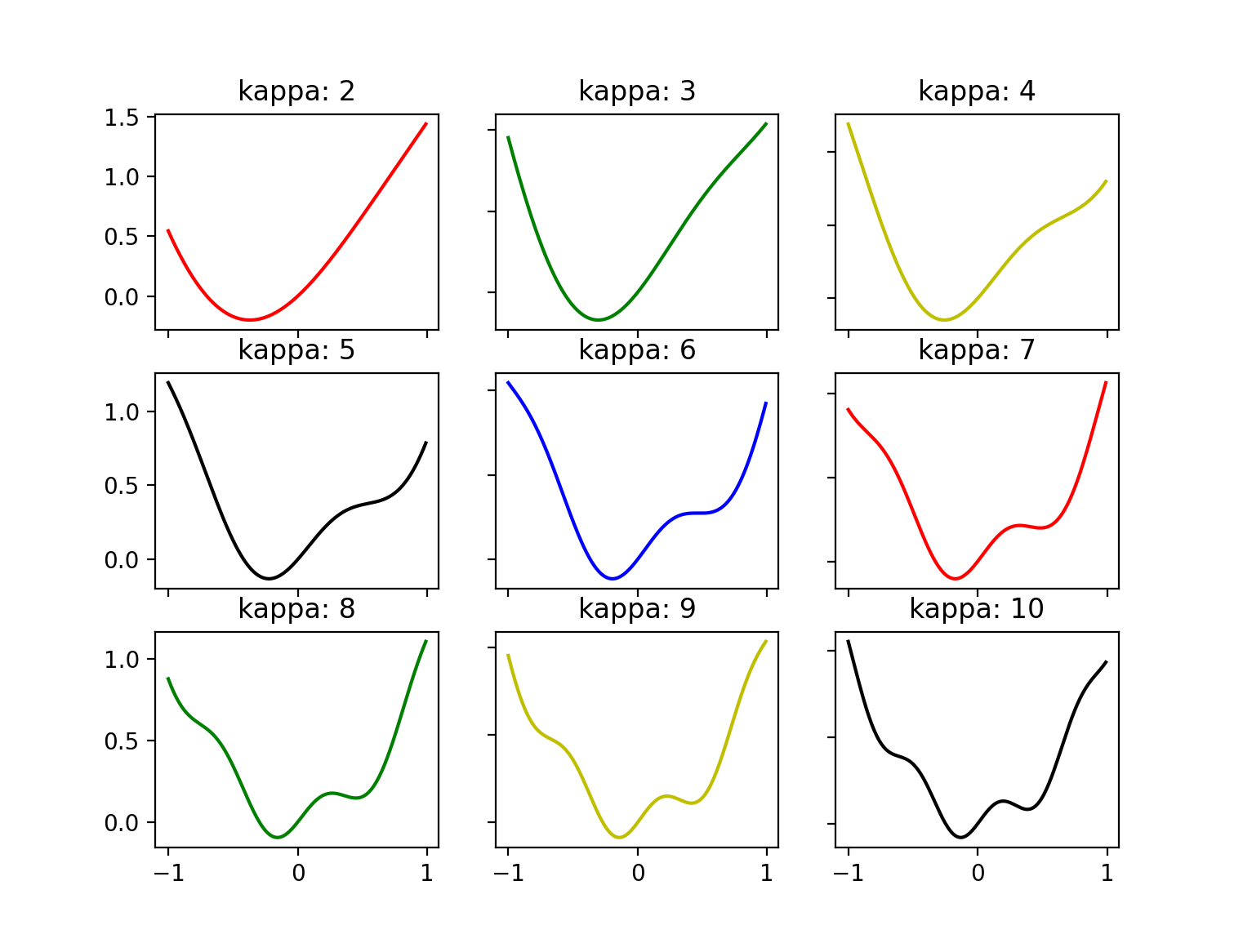
(a) Evolution of ${\mathscr{J}}$ with $\kappa$.

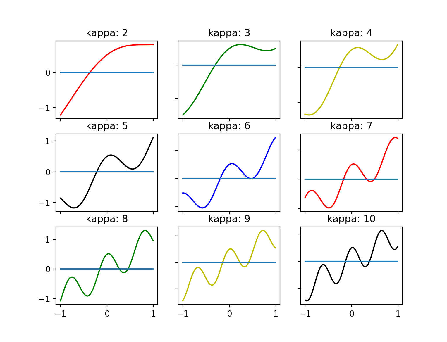
(b) Evolution of $\frac{\mathrm{d}}{\mathrm{d}\beta}{\mathscr{J}}$ with $\kappa$.

Figure 5. Minimizers of the mean field control problem and equilibria of the mean field game for $\kappa\in\{2,\cdots,10\}$ when $d=1$ and $g(x)=\cos(\kappa x)$: Solutions of the mean field control problem are the minimizers of ${\mathcal{J}}$; Solutions of the mean field game are the roots of $\frac{\mathrm{d}}{\mathrm{d}\beta}{\mathscr{J}}$.

Interestingly, the recent contribution [24] says that, when the MFG is potential, the equilibria that are not associated with a minimizer of the potential should be ruled out. Equivalently, only the MFG solutions that minimize (globally) the potential should be selected. Even more, the guess (which has been rigorously established in [24, 32] but in different settings that the one addressed here) is that the minimizers of the potential are precisely those that appear by forcing uniqueness with a common noise and then by tuning down the intensity of the common noise. We check this prediction numerically in Subsection 3.5, by using our learning method.

3.2. Algorithms for a fixed intensity of the common noise

We here explain how to implement the fictitious play in the two benchmark examples (3.2) and (3.3) along the lines of Figure 3. Throughout the subsection, the intensity of the common noise is fixed. For simplicity, the intensity of the common noise is chosen as $\varepsilon=1$ and the intensity of the independent noise is chosen as $\sigma=0$ or $1$. Numerical experiments are discussed in the next subsection.

3.2.1. Numerical reference solution

We first explain how to compute a reference solution by solving numerically the decoupled forward-backward equation (2.11). Observe that there is no contradiction in using a numerical method for testing our learning algorithm: the numerical method relies on the explicit knowledge of the coefficient $g$, whereas the learning algorithm is intended to work on the sole observations of the costs.

The numerical method we use is tailor-made to our problem. Indeed, we observe that the solution to the backward equation in (2.15) writes

$$h_{t}={\mathbb{E}}^{{\bm{h}}}\biggl{[}\exp\biggl{(}-\int_{t}^{1}\eta_{s}\mathrm{d}s\biggr{)}g\bigl{(}m_{1}\bigr{)}\,\big{|}\,{\mathcal{F}}^{{\bm{W}}}_{t}\biggr{]},\quad t\in[0,1],$$ (3.10)

where $(m_{t})_{0\leq t\leq 1}$ is an Ornstein-Uhlenbeck process (with independent coordinates)

$$\mathrm{d}m_{t}=-\eta_{t}m_{t}\mathrm{d}t+\mathrm{d}W_{t},\quad t\in[0,1]\ ;\quad m_{0}=0.$$ (3.11)

We then employ a Picard scheme for solving the fixed point equation (3.10), by iterating

$$h_{t}^{\textrm{\rm ref},n+1}={\mathbb{E}}^{{\bm{h}}^{\textrm{\rm ref},n}}\biggl{[}\exp\biggl{(}-\int_{t}^{1}\eta_{s}\mathrm{d}s\biggr{)}g\bigl{(}m_{1}\bigr{)}\,\big{|}\,{\mathcal{F}}^{{\bm{W}}}_{t}\biggr{]},\quad t\in[0,1],$$ (3.12)

Numerically, we use a time grid $\{t_{k}=k/p\}_{k}$ with $p$ uniform steps (for the same $p$ as the one used in the learning method, which makes the comparison easier) and, following the seminal work of [42], we employ a regression method in order to approximate the conditional expectation appearing in the right-hand side. Precisely, we find, at each iteration $n$ of the Picard sequence and at each node $t_{j}>0$ of the time mesh, an approximation of the conditional expectation in the right-hand side of (3.12) in the form of a (deterministic) function of $m_{t_{j}}$ (the forward component in (3.12)), with the deterministic function being chosen in a given class of functions from ${\mathbb{R}}^{d}$ into itself. The point is then to choose a convenient class within which the regression is achieved.

Here, we address two approaches, already reported in the literature. The first one consists in performing regression on linear combinations of Hermite polynomials. It is inspired from [11], which offers (in a somewhat more complicated framework) some theoretical bounds on the regression error. The second approach is taken from the work [37], which paved the way for a systematic use of neural networks in the computation of numerical solutions to nonlinear PDEs and related Markovian BSDEs. The point in this second approach is thus to approximate the conditional expectation in (3.12), at time $t=t_{j}$, by means of a neural network with $m_{t_{j}}$ as entry.

For the sake of completeness, we provide of a short overview of the shape of the functions within these two classes.

Using Hermite polynomials. The real-valued components of the regression functions are taken in the linear span of $\{H_{\ell}^{d}(\cdot/\sigma_{t_{j}})\}_{|\ell|\leq D}$, where $\sigma_{t_{j}}$ is the common standard deviation of the coordinates of $m_{t_{j}}$ (which is explicitly computable) and $\{H_{\ell}^{d}(\cdot)\}_{|\ell|\leq D}$ is the collection of Hermite polynomials of dimension $d$ ($d=1,2$ in our case) and of degree less than $D$, for a given integer $D$ (here $\ell$ is a $d$-tuple of integers and $|\ell|$ is the sum of its entries). We recall that, when $d=1$,

$$H_{\ell}^{1}(x)=\frac{(-1)^{\ell}}{\sqrt{2^{\ell}\ell!}}e^{x^{2}}\frac{\mathrm{d}}{\mathrm{d}x^{\ell}}[e^{-x^{2}}],\quad x\in{\mathbb{R}}.$$

When $d=2$,

$$H_{(\ell_{1},\ell_{2})}^{2}(x_{1},x_{2})=H_{\ell_{1}}^{1}(x_{1})H_{\ell_{2}}^{1}(x_{2}),\quad x_{1},x_{2}\in{\mathbb{R}}.$$

Using a neural network. For a number of layers $L$, the functions used for the regression have the form $\psi^{L+1}\circ\varphi^{L}\circ\psi^{L}\cdots\circ\psi^{2}\circ\varphi^{1}\circ\psi^{1}$, with $\psi^{\ell}$, for each $\ell=1,\cdots,L+1$, being an affine function from ${\mathbb{R}}^{d_{\ell-1}}$ to ${\mathbb{R}}^{d_{\ell}}$, where $d_{0}=d_{L+1}=d$. For each $\ell=1,\cdots,L$, $\varphi^{\ell}$ is a function from ${\mathbb{R}}^{d_{\ell}}$ into itself that maps $(x_{1},\cdots,x_{d_{\ell}})$ onto $(\varsigma(x_{1}),\cdots,\varsigma(x_{d_{\ell}}))$ for some activation function $\varsigma$ (which, for simplicity, is taken to be the same for any $\ell$). The activation function is fixed a priori. Standard examples for it are the ReLu or Sigmoid functions. We then call neurons of the networks the coefficients encoding the linear mappings $(\psi^{\ell})_{\ell=1,\cdots,L+1}$. In clear, the principle is to tune, for each $\ell$, matrices $A^{\ell}\in{\mathbb{R}}^{d_{\ell-1}\times d_{\ell}}$ and vectors $B^{\ell}\in{\mathbb{R}}^{d_{\ell}}$ in the decomposition of $\psi_{\ell}$ as

$$\psi^{\ell}(x)=A^{\ell}x+B^{\ell},\quad x\in{\mathbb{R}}^{d_{\ell-1}}.$$

Neural networks are notoriously known to (possibly) behave well in higher dimension. Below, we provide examples with $d=12$ and $d=20$.

Given a finite dimensional class ${\mathcal{C}}$ of regression functions (obtained by Hermite polynomials or neural networks), we use the following algorithm for the the computation of a reference solution.

Algorithm 1. [Reference solution]

1. Introduce $\Delta_{t_{k}}w^{(j)}$ with $j\in\{1,\cdots,N\}$ and $k\in\{1,\cdots,p\}$, a collection of $N$ realizations of independent Gaussian variables ${\mathcal{N}}(0,I_{d})$.

2. For each $i$, compute $(m^{(j)}_{t_{k}})_{j=0,\cdots,p}$ the realizations of the Euler scheme associated with (3.11) and driven by the simulations

   $$\biggl{(}w^{(j)}_{t_{k}}=\frac{1}{\sqrt{p}}\Bigl{[}\Delta_{t_{1}}w^{(j)}+\cdots+\Delta_{t_{k}}w^{(j)}\Bigr{]}\biggr{)}_{k=1,\cdots,p}.$$

3. One iteration consists of one Picard iteration. The input at iteration number $n$ is encoded in the form of an array $(h_{t_{k}}^{n,(j)})_{j,k}$ with entries in ${\mathbb{R}}^{d}$. The following procedure returns the next input for iteration number $n+1$.

   1. Look for $(h_{t_{k}}^{n+1,(j)})_{j,k}$ in terms of $(h_{t_{k}}^{n,(j)})_{j,k}$ by solving, for each $k=0,\cdots,p-1$, the minimization problem

      $$\min_{{\mathfrak{h}}\in{\mathcal{C}}}\frac{1}{N}\sum_{j=1}^{N}{\mathcal{E}}^{n,(j)}_{k}\biggl{|}\exp\biggl{(}-\sum_{s=k}^{p-1}\eta_{t_{s}}\biggr{)}g(m_{1}^{(j)})-{\mathfrak{h}}\bigl{(}m_{t_{k}}^{(j)}\bigr{)}\biggr{|}^{2},$$

      with

      $${\mathcal{E}}^{n,(j)}_{k}=\exp\biggl{(}-\sum_{s=k}^{p-1}h_{t_{s}}^{n,(j)}\cdot\Delta_{t_{k+1}}w^{(j)}-\frac{1}{2p}\sum_{s=k}^{p-1}|h_{t_{s}}^{n,(j)}|^{2}\biggr{)}.$$

   2. To enforce some stability, update each coordinate of $(h_{t_{k}}^{n+1,(j)})_{j,k}$ by projecting it onto $[-1,1]$.

Remark 3.2.

For instance, when Hermite polynomials are used, the minimization step in Algorithm 1 can be rewritten as

$$\min_{{\bm{c}}=(c_{\ell})_{|\ell|\leq D}}\frac{1}{N}\sum_{j=1}^{N}{\mathcal{E}}^{n,(j)}_{k}\biggl{|}\exp\biggl{(}-\sum_{s=k}^{p-1}\eta_{t_{s}}\biggr{)}g(m_{1}^{(j)})-\sum_{|\ell|\leq D}c_{\ell}H^{d}_{\ell}\bigl{(}\tfrac{1}{\sigma_{t_{k}}}m_{t_{k}}^{(j)}\bigr{)}\biggr{|}^{2},$$

where each $c_{\ell}$ in ${\bm{c}}=(c_{\ell})_{|\ell|\leq D}$ is in ${\mathbb{R}}^{d}$. (When $k=0$, only $c_{\bm{0}}$, where $|{\bm{0}}|=0$, matters and it is given by a mere empirical mean.)

Here, the coordinates in (3.11) have the same marginal variances because $(\eta_{t})_{0\leq t\leq T}$ is scalar-valued (or equivalent is a $d$-diagonal matrix). This is no longer true when $R$ and $Q$ in (1.2) are general matrices. In such a case (and more generally when the components are not centered), the components of $(m_{t})_{0\leq t\leq T}$ are no longer independent and the ‘normalized’ Hermite polynomials $\{H_{\ell}^{d}(\cdot/\sigma_{t_{k}})\}_{|\ell|\leq D}$ used above should be instead replaced by $\{H_{\ell}^{d}({\mathbb{K}}^{-1/2}(m_{t_{k}})(\cdot-{\mathbb{E}}(m_{t_{k}}))\}_{|\ell|\leq D}$, where ${\mathbb{K}}(m_{t_{j}})$ is the covariance matrix of $m_{t_{k}}$ and ${\mathbb{K}}^{1/2}(m_{t_{k}})$ is any root of it (e.g., as given by the Cholesky decomposition).

3.2.2. Numerical approximation by fictitious play

We now address the implementation of the fictitious play according to the principle stipulated by Figure 3. The black-box therein is discretized in a suitable manner. It is used to solve numerically the optimization problem (2.32), and then to implement the updating rule (2.45) for the environment. Since Lemma 2.13 says that the corresponding optimal law has an affine Markov feedback form, we can perform the optimization in (2.32) over closed loop controls that are affine in the state variable, with the linear coefficient being a scalar only depending on time and with the intercept possibly depending on the environment. From the practical point of view, this choice is fully justified if the model is expected to be linear-quadratic in the space/action variables (as it is in (1.1)–(1.2), with $Q$ and $R$ being scalars), but this does not require the coefficients $Q$, $R$, $f$ and $g$ to be known explicitly. Mathematically, this writes as follows. We can restrict ourselves to controls ${\bm{\alpha}}=(\alpha_{t_{k}})_{{k=1,\cdots,p}}$ of the form

$$\alpha_{t_{k}}=a_{t_{k-1}}X_{t_{k-1}}+C_{t_{k-1}},$$ (3.13)

where $a_{t_{k-1}}$ is a scalar and $C_{t_{k-1}}$ is a $d$-dimensional random vector (which is typically adapted to the increments $(\Delta_{t_{\ell}}w)_{\ell\leq k-1}$, but the measurability properties of which are specified in a finer manner right below). In comparison with the formula (2.37), $a_{t_{k-1}}$ should be understood as a proxy for $-\eta_{t_{k-1}}$ and $C_{t_{k-1}}$ as a proxy for the intercept therein. Part of the numerical difficulty is thus to have a tractable regression method for capturing the randomness of $C_{t_{k-1}}$. Recalling that the intercept ${\bm{h}}$ in the solution of the mean field game with common noise is a function of the environment $(m_{t})_{0\leq t\leq 1}$, see (2.18), a key point in our numerical method is to look for $C_{t_{k-1}}$ as a $\sigma(\overline{m}_{t_{k-1}})$-measurable random variable, where $\overline{m}_{t_{k-1}}$ is the current proxy for the state of the environment at time $t_{k-1}$. Numerically, we use a regression method, very much in the spirit of Algorithm 1: either we use a regression based on a $d$-dimensional linear combination of Hermite polynomials of degree less than $D$, for a fixed value of $D$, or we use a neural network with $L$ layers and with a prescribed numbers of neurons. Of course, the reader may wonder about another approach to (3.13), in which we optimize over general (possibly non-affine) controls in Markov feedback form. In fact, while this seems an attractive way to bypass any a priori knowledge about the shape of the model, this approach requires an extra step for updating the intercept ${\bm{h}}$ at the next iteration of the fictitious play. Intuitively, the new intercept value can be found by linearly regressing the controls on the states. At this point, however, we assert that the presence of this additional step in the numerical procedure can only be fully justified if the linear-quadratic structure of the model is known. This makes the advantage of not postulating (3.13) very limited.

We now make this construction explicit when $\sigma=\varepsilon=1$ and the postulate (3.13) is in force, noticing that the algorithm must rely on simulations for the independent and common noises. Throughout, the learning parameter $\varpi$ is arbitrary: it may be strictly greater than 1 (in which case we are using the geometric variant of the fictitious play) or equal to 1 (in which case we are using the harmonic variant). Below, we call $M$ the number of particles (given a realization of the common noise) and $N$ the number of simulations of the whole system (or equivalently of the common noise), with $i$ denoting the generic label for a particle and $j$ denoting the generic label for a realization. We are thus given a collection

$$\Delta_{t_{k}}b^{(i,j)},\ \Delta_{t_{k}}w^{(j)},\quad i\in\{1,\cdots,M\},\ j\in\{1,\cdots,N\},\ k\in\{1,\cdots,p\},$$ (3.14)

of realizations of independent ${\mathcal{N}}(0,I_{d})$ Gaussian variables. At iteration number $n$ of the fictitious play, the current proxy for the environment is thus given in the form of a collection $(\overline{m}^{n,(j)}_{t_{k}})_{j,k}$, with $j$ running from $1$ to $N$ and $k$ running from $0$ to $p$. Similarly, the proxy for the intercept in the optimal law (2.37) is given in the form of a collection $(h^{n,(j)}_{t_{k}})_{j,k}$, also with $j$ running from $1$ to $N$ and $k$ running from $0$ to $p-1$. The fact that the two proxies are independent of $i$ is fully consistent with the fact that $\overline{\bm{m}}^{n}$ and ${\bm{h}}^{n}$ in Remark 2.16 are adapted to the realization of the common noise. Following our introductory discussion, we solve, as an approximation of the stochastic control problem (2.32), the minimization problem:

$$\min\biggl{\{}\frac{1}{N}\sum_{j=1}^{N}\biggl{(}{\mathcal{E}}^{n,(j)}\frac{1}{M}\sum_{i=1}^{M}\biggl{[}\frac{1}{2p}\sum_{k=1}^{p}\varpi^{2}|\alpha_{t_{k}}^{(i,j)}|^{2}+\frac{1}{2}\Bigl{|}\varpi x^{(i,j)}_{1}+g\Bigl{(}\overline{m}_{1}^{n,(j)}\Bigr{)}\Bigr{|}^{2}\biggr{]}\biggr{)}\biggr{\}},$$ (3.15)

where

$${\mathcal{E}}^{n,(j)}=\exp\Biggl{(}-\varpi\sqrt{\frac{1}{p}}\sum_{k=0}^{p-1}h^{n,(j)}_{t_{k}}\cdot\Delta_{t_{k+1}}w^{(j)}-\frac{\varpi^{2}}{2p}\sum_{k=0}^{p-1}|h^{n,(j)}_{t_{k}}|^{2}\Biggr{)}.$$

Moreover, in the minimization problem, $\alpha_{t_{k}}^{(i,j)}$, $x_{t_{k}}^{(i,j)}$ are required to be of the form

$$\begin{split}&x_{t_{k}}^{(i,j)}=x_{t_{k-1}}^{(i,j)}+\frac{1}{p}\alpha_{t_{k}}^{(i,j)}+{\frac{1}{\varpi\sqrt{p}}}\Delta_{t_{k}}b^{(i,j)},\quad\ell=1,\cdots,p\ ;\quad x_{0}^{(i,j)}=x_{0},\\ &\alpha_{t_{k}}^{(i,j)}=a_{t_{k-1}}x_{t_{k-1}}^{(i,j)}+C_{t_{k-1}}^{(j)}+\varpi h^{n,(j)}_{t_{k-1}}+\sqrt{p}\Delta_{t_{k}}w^{(j)},\quad k=1,\cdots,p.\end{split}$$ (3.16)

In particular, $(x_{t_{k}}^{(i,j)})_{k=0,\cdots,p}$ solves the following Euler scheme:

$$x_{t_{k}}^{(i,j)}=x_{t_{k-1}}^{(i,j)}+\frac{1}{p}\Bigl{(}a_{t_{k-1}}x_{t_{k-1}}^{(i,j)}+C_{t_{k-1}}^{(j)}+\varpi h^{n,(j)}_{t_{k-1}}\Bigr{)}+{\frac{1}{\varpi\sqrt{p}}}\Delta_{t_{k}}b^{(i,j)}+{\frac{1}{\sqrt{p}}}\Delta_{t_{k}}w^{(j)},\quad k=1,\cdots,p.$$

Moreover, $C^{(j)}_{t_{k}}$ is required to be of the form

$$C^{(j)}_{t_{k}}={\mathfrak{h}}_{t_{k}}\bigl{(}\overline{m}^{n,(j)}_{t_{k}}\bigr{)},$$ (3.17)

for a function ${\mathfrak{h}}_{t_{k}}$ within one of the two classes ${\mathcal{C}}$ described in Subsection 3.2.1, depending on whether we use Hermite polynomials or neural networks. As already explained, neural networks may provide better results in higher dimension (or, to put it differently, Hermite polynomials may be of an intractable complexity in higher dimension).

As before, we feel useful to exemplify (3.17) within each of the two aforementioned case.

Using Hermite polynomials. In this case, we use a slightly modified form of (3.17), as we also center $\overline{m}^{n,(j)}_{t_{k}}$ by means of the empirical mean in the argument of the Hermite polynomials. Definition (3.17) thus becomes:

$$C^{(j)}_{t_{k}}=\sum_{|\ell|\leq D}c_{t_{k}}(\ell)H^{d}_{\ell}\biggl{(}\bigl{(}U_{t_{k}}^{n}\bigr{)}^{-1}\Bigl{(}\overline{m}^{n,(j)}_{t_{k}}-\frac{1}{N}\sum_{r=1}^{N}\overline{m}^{n,(r)}_{k}\Bigr{)}\biggr{)},$$ (3.18)

where $c_{k}(\ell)\in{\mathbb{R}}^{d}$ and $U_{t_{k}}^{n}$ is the diagonal matrix obtained by taking the roots of the diagonal of the empirical covariance matrix:

$$\Sigma_{t_{k}}^{n}=\frac{1}{N}\sum_{j=1}^{N}\Bigl{(}\overline{m}^{n,(j)}_{t_{k}}-\frac{1}{N}\sum_{r=1}^{N}\overline{m}^{n,(r)}_{t_{k}}\Bigr{)}\otimes\Bigl{(}\overline{m}^{n,(j)}_{t_{k}}-\frac{1}{N}\sum_{r=1}^{N}\overline{m}^{n,(r)}_{t_{k}}\Bigr{)}.$$

Remark 3.3.

Following Remark 3.2, we can define $U_{t_{k}}^{n}$ (in a more general fashion) as the upper triangular matrix given by the Cholesky decomposition of $\Sigma_{t_{k}}^{n}$ in the form $\Sigma_{t_{k}}^{n}=(U_{t_{k}}^{n})^{\dagger}U_{t_{k}}^{n}$.

The minimization problem in (3.15) is thus defined (when using Hermite polynomials) over ${\bm{a}}=(a_{t_{k}})_{k}\in{\mathbb{R}}^{p}$ and ${\bm{c}}=(c_{t_{k}}(\ell))_{k,\ell}\in({\mathbb{R}}^{d})^{p\times L}$, where $L$ is the number of distinct $d$-tuples of (non-negative) integers whose sum is less than $D$.

Using neural networks. With the same definition as in Subsection 3.2.1, (3.17) takes the form

$$C^{(j)}_{t_{k}}=\psi^{L+1}_{t_{k}}\circ\varphi^{L}_{t_{k}}\circ\psi^{L}_{t_{k}}\cdots\circ\psi^{2}_{t_{k}}\circ\varphi^{1}_{t_{k}}\circ\psi^{1}_{t_{k}}\bigl{(}\overline{m}^{n,(j)}_{t_{k}}\bigr{)}.$$ (3.19)

Typically, the number of layers $L$, the dimensions of the various layers and the activation functions are the same for any time $t_{k}$, $k=0,\cdots,N-1$. In other words, we can write $\varphi^{L}_{t_{k}}=\varphi^{L}$, $\varphi^{L-1}_{t_{k}}=\varphi^{L-1}$, $\cdots$. Each $\psi_{t_{k}}^{\ell}$, for $\ell=1,\cdots,L+1$, writes as

$$\psi_{t_{k}}^{\ell}(x)=A_{k}^{\ell}x+B_{k}^{\ell},\quad x\in{\mathbb{R}}^{d_{\ell-1}}.$$

The minimization problem in (3.15) is thus defined over ${\bm{a}}=(a_{t_{k}})_{k}\in{\mathbb{R}}^{p}$, ${\bm{A}}=(A_{k}^{\ell})_{k,\ell}$ and ${\bm{B}}=(B_{k}^{\ell})_{k,\ell}$, with $A_{k}^{\ell}\in{\mathbb{R}}^{d_{\ell-1}\times d_{\ell}}$ and $B_{k}^{\ell}\in{\mathbb{R}}^{d_{\ell}}$.

We can summarize the algorithm in the following form. It has the same form whether we work with the harmonic ($\varpi=1$) or geometric ($\varpi>1$) version of the fictitious play.

Algorithm 2. [Learning with two noises, $\sigma=\varepsilon=1$]

1. Take as input the realizations (3.14), which are the same at any iteration of the algorithm.

2. At rank $n+1$ of the fictitious play:

   1. Take as input the proxies $(\overline{m}^{n,j}_{t_{k}})_{j,k}$ and $(h^{n,j}_{t_{k}})_{j,k}$ for (respectively) the environment and the intercept.

   2. Solve the minimization problem (3.15) over ${\bm{a}}=(a_{t_{k}})_{k}$ in (3.16) and ${\bm{\mathfrak{h}}}=({\mathfrak{h}}_{t_{k}})_{k}$ in (3.17). Call ${\bm{a}}^{n+1}=(a^{n+1}_{t_{k}})_{k}$ and ${\bm{\mathfrak{h}}}^{n+1}=({\mathfrak{h}}^{n+1}_{t_{k}})_{k}$ the optimal points (returned by any optimization method).

   3. With ${\bm{a}}^{n+1}=(a_{t_{k}}^{n+1})_{k}$ and ${\bm{\mathfrak{h}}}^{n+1}=({\bm{\mathfrak{h}}}^{n+1}_{t_{k}})_{k}$, associate $(x^{n+1,(i,j)}_{t_{k}})_{i,j,k}$ as in (3.16) and $(C_{t_{k}}^{n+1,(j)})_{k,j}$ as in (3.17).

   4. Update the proxies by letting

      $$\begin{split}&m^{n+1,(j)}_{t_{k}}=\frac{1}{M}\sum_{i=1}^{M}x^{n+1,(i,j)}_{t_{k}},\quad\overline{m}^{n+1,(j)}_{t_{k}}=\pi_{n+1}(\varpi)\times m^{n+1,(j)}_{t_{k}}+\bigl{(}1-\pi_{n+1}(\varpi)\bigr{)}\times\overline{m}^{n,(j)}_{t_{k}},\\ &h^{n+1,(j)}_{t_{k}}=-C_{t_{k}}^{n+1,(j)},\end{split}$$

   where $\displaystyle\pi_{n}(\varpi)=\left\{\begin{array}[]{ll}1/n&{\rm if}\ \varpi=1,\\ \tfrac{\varpi^{-(n-1)}(1-\varpi^{-1})}{1-\varpi^{-n}}&{\rm if}\ \varpi>1.\end{array}\right.$

Remark 3.4.

The construction of Algorithm 2 relies on the various noises (3.14). In fact, it is worth mentioning that the algorithm can be reformulated in a similar manner when the increments $(\Delta_{t_{k}}b^{(i,j)})_{i,j,k}$ defining the idiosyncratic noises are assumed to just depend on $(i,k)$ (equivalently they are equal for the same value of $i$ but for two different values of $j$). As before, the resulting random variables $(\Delta_{t_{k}}b^{(i)})_{i=1,\cdots,M,k=1,\cdots,p}$ are required to be independent and identically distributed.

Obviously, the smallest family $(\Delta_{t_{k}}b^{(i)})_{i=1,\cdots,M,k=1,\cdots,p}$ is of a cheapest numerical cost. However, it creates additional correlations between the particles: for two different indices $j$ and $j^{\prime}$, the corresponding two empirical means over $i\in\{1,\cdots,N\}$ in (3.15) are dependent, with the correlations vanishing asymptotically as $N$ tends to $\infty$. Even though we do not provide any bound for the numerical error in this section, it is worth mentioning that the presence of additional correlations would make the Monte-Carlo error harder to estimate. As reported below, we tested the two approaches. For the range of parameters we used, we have not seen any major difference.

In some of the numerical examples below, we will use variants of Algorithm 2. We first focus on the shape of the algorithm when $\sigma=0$, recalling that our results do not require the presence of an idiosyncratic noise. Implicitly, we then have a single particle only, i.e. $M=1$. Moreover, $\Delta_{t_{k}}b^{(i,j)}$ no longer appears in (3.16). We then have the following variant of Algorithm 2, which is of lower complexity:

Algorithm 3. [Learning with common noise only, $\sigma=0$, $\varepsilon=1$]

1. Take as input the realizations $(\Delta_{t_{k}}w^{(j)})_{j,k}$ in (3.14), which are the same at any iteration of the algorithm.

2. At rank $n+1$ of the fictitious play, apply the same loop as in Algorithm 2, but with $M=1$ and with $\Delta_{t_{k}}b^{(1,j)}=0$ in (3.16).

We end up our presentation with the case when there is no common noise, i.e. $\sigma=1$ and $\varepsilon=0$. In that case, our strategy no longer applies. The point is thus to implement the standard version of the fictitious play. Accordingly, there is no Girsanov density in (3.15) and $\alpha_{t_{k}}^{(i,j)}$ in (3.16) merely writes

$$\alpha_{t_{k}}^{(i,j)}=a_{t_{k-1}}x_{t_{k-1}}^{(i,j)}+C_{t_{k-1}},\quad k=1,\cdots,p.$$

with $C_{t_{k}}$ being a deterministic $d$-dimensional vector (which is independent of $j$). In particular, there is no need to use the proxy $(h^{n,j}_{t_{k}})_{j,k}$ for the intercept. Equivalently, we can assume that $N=1$ and ${\mathfrak{h}}_{t_{k}}$ in (3.17) to be a mere constant function (i.e., the function ${\mathfrak{h}}_{t_{k}}$ is identified with ${\mathfrak{h}}_{t_{k}}(0)$). The rest of the algorithm is similar. It may be written as follows.

Algorithm 4. [Learning with idiosyncratic noise only, $\sigma=1$, $\varepsilon=0$]

1. Take as input the realizations $(\Delta_{t_{k}}b^{(i,1)})_{k}$ in (3.14), which are the same at any iteration of the algorithm.

2. At rank $n+1$ of the fictitious play:

   1. Take as input the proxy $(\overline{m}^{n}_{t_{k}})_{k}$ for the environment and the intercept.

   2. Solve the minimization problem (3.15) over ${\bm{a}}=(a_{t_{k}})_{k}$ in (3.16) and ${\bm{\mathfrak{h}}}=({\mathfrak{h}}_{t_{k}})$ in (3.17), with ${\mathcal{E}}^{n,(j)}=1$ in (3.15) and with the last line in (3.16) being replaced by

      $$\alpha_{t_{k}}^{(i,1)}=a_{t_{k-1}}x_{t_{k-1}}^{(i,1)}+{\mathfrak{h}}_{t_{k-1}}(0),\quad k=1,\cdots,p.$$

      Call ${\bm{a}}^{n+1}=(a^{n+1}_{t_{k}})_{k}$ and ${\bm{\mathfrak{h}}}^{n+1}(0)=({\mathfrak{h}}^{n+1}_{t_{k}}(0))_{k}$ the optimal points.

   3. With ${\bm{a}}^{n+1}=(a_{t_{k}}^{n+1})_{k}$ and ${\bm{\mathfrak{h}}}^{n+1}=({\mathfrak{h}}^{n+1}_{t_{k}}(0))_{k}$, associate $(x^{n+1,(i,1)}_{t_{k}})_{i,k}$ as in (3.16) (with the same prescription as above).

   4. Update the proxy by letting

      $$\begin{split}&m^{n+1,(1)}_{t_{k}}=\frac{1}{M}\sum_{i=1}^{M}x^{n+1,(i,1)}_{t_{k}},\quad\overline{m}^{n+1,(1)}_{t_{k}}=\pi_{n+1}(\varpi)m^{n+1,(1)}_{t_{k}}+\bigl{(}1-\pi_{n+1}(\varpi)\bigr{)}\overline{m}_{t_{k}}^{n,(1)},\end{split}$$

      with $\pi_{n}(\varpi)$ being defined as in Algorithm 2.

In all the numerical experiments, we use ADAM optimizer (as implemented in TensorFlow) in order to solve the optimization step in Algorithms 2, 3 and 4. We recall from the discussion in Subsection 1.7 that the code in TensorFlow relies on some automatic differentiation and thus makes an explicit use of the linear-quadratic form of the coefficients. In this sense, our numerical implementation requires part of the model to be known, but, as we already explained in Subsection 1.7, this does not really affect the scope of our conclusions: Provided the optimization method used in Algorithms 2, 3 and 4 is sufficiently accurate, the whole works well and demonstrates the interest for exploring the state space by means of the common noise.

3.3. Numerical experiments in low dimension

The numerical examples that we provide below are here to illustrate several features of our form of fictitious play. In all the examples treated in this subsection, we choose $d=2$, $f\equiv 0$ and $g$ as in (3.3) with $\kappa=10$. The intercept ${\bm{h}}^{n}$ in (2.32) is approximated by means of Hermite polynomials, as explained in Subsection 3.2.1. Similar conclusions to the ones that are reported here could be drawn if the regression of ${\bm{h}}^{n+1}$ onto $\overline{\bm{m}}^{n}$ (see (3.17)) was done by using a neural network. For brevity, we feel however more appropriate to restrict the exposition of the numerical results obtained with neural networks to the higher dimensional setting only, which is done in the next section.

It is worth mentioning that, whatever the method that is used, our aim is to demonstrate, numerically, the positive impact of the common noise, but not to compare the numerical rates of convergence obtained in the numerical experiments with the bounds obtained in the theoretical analysis. The reason is that the algorithms we present below include additional features (like numerical optimization methods and regressions) that are not addressed in the theoretical analysis. This makes difficult any precise comparison. Also, it is fair to say that the time of execution of the full algorithm becomes quite long (several hours for the longest experiments), even for low values of $n$ and $p$ ($n$ less than 50 and $p$ less than 100).

As for the parameter $\varpi$, we address its influence in several manners. To do so, we implement both the harmonic and geometric variants of the fictitious play. Even in the harmonic regime (i.e., $\varpi=1$), we can easily see the impact of the common noise, especially when the latter has intensity 1 (which is our choice in this subsection). Obviously, this is very good. A related observation is that, although our theoretical guarantees (given by the analogues of Theorems 2.4 and 2.17 in the harmonic regime, see Remark 2.6) just provide a harmonic decay when $\varpi=1$, the observed rate of convergence may be better. In particular, the difference with the geometric version is rather tiny on the examples that are tested in this subsection, for a common noise with intensity 1 (as we will see in the forthcoming Subsection 3.5, the picture is different when the viscosity is small). There are even situations where, for numerical reasons, the harmonic variant has better results than the geometric one. For sure, this could be rather surprising for the reader (and even disappointing in some sense), but it is clear that our (theoretical) estimates rely on rather generic properties of the dynamics in hand. Obviously, there might be more subtle features of the equations that should be taken into account in order to explain the behavior of the algorithm as the number $n$ of iterations of the fictitious play increases. Having a sharp understanding of the algorithm when $n$ is large and, at the same time, $\varepsilon$ is small is even more difficult. As we already explained, the constant $\exp(C\varepsilon^{-2})$ that appears in all of our estimates is certainly non-optimal in many situations.

3.3.1. Evolution of the learnt cost with one type of noise only

We first test the influence of each of the two types of noises onto the behavior of the algorithm. We thus compare the evolution of the cost learnt by the harmonic and geometric fictitious plays in three scenarios (Figure 6): In the first scenario, there is an independent noise, but no common noise (Algorithm 4); in the second scenario, there is a common noise but no independent noise and $\varpi=1$ (Algorithm 3, harmonic fictitious play); in the third scenario, there is a common noise but no independent noise and $\varpi=1.1$ (Algorithm 3, geometric fictitious play).

(a) With independent but no common noise

(b) With common but no independent noise, $\varpi=1$

(c) With common but no independent noise, $\varpi=1.1$

Figure 6. Harmonic and geometric fictitious plays. Comparison of the learnt cost depending on the type of noise and the value of $\varpi$. In $x$-axis: number of iterations; In $y$-axis; learnt cost.

The experiments are computed with: $n=20$ learning iterations, $p=30$ time steps, $M=4\times 10^{5}$, $N=1$, $\sigma=1$ and $\varepsilon=0$ in case (A) and $n=p=20$, $M=1$, $N=4\times 10^{5}$, $\sigma=0$, $\varepsilon=1$ and $D=4$ in cases (B) and (C). In ADAM method, the learning rate is $0.01$, with 15 epochs and one batch.

In plots (B) and (C), the orange line is the theoretical equilibrium cost as computed by the BSDE method explained in Subsection 3.2.1. In plot (A), there is no computed reference cost. As we already explained, there might not be a unique equilibrium and the notion of reference cost no longer makes sense. Notice by the way that the equilibrium cost in cases (B) and (C) is not an equilibrium cost in case (A) because the problems are different (as being set over different forms of dynamics). Anyway, the conclusion is clear: the learnt cost exhibits an oscillatory behavior in case (A), whereas it does not in cases (B) and (C). This is an evidence of the numerical impact of the common noise onto the behavior of the fictitious play. Of course, it would be desirable to have more theoretical guarantees on the possible divergence of the fictitious play in absence of the common noise. Unfortunately, we are not aware of such results. In our numerical experiments (including some that are not reported here), we have been able to reproduce the oscillatory behavior characterizing the pane (A) in Figure 6 in other two-dimensional examples without common noise, meaning that, for a given batch (even of large size), the learnt (or training) cost may feature some non-trivial oscillations. However, we have not been able to reproduce a similar phenomenon in dimension 1 (in which case the fictitious play is known to converge), even when the MFG is known to have multiple equilibria. As for panes (B) and (C), it is worth observing that the results are consistent. As announced, the convergence is fast, even in case (B), for which our theoretical guarantees just provide a harmonically decaying bound for the error.

3.3.2. Error in the optimal path/intercept with common noise and no independent noise

We now compute the error achieved by the learning algorithm. Using the same notation as in the statement of Theorem 2.17, we focus on the following $L^{2}$ error:

$$\biggl{[}{\mathbb{E}}\int_{0}^{1}\Bigl{(}|\overline{m}_{t}^{n}-m_{t}^{(p)}|^{2}+|\varpi h_{t}^{n}-h_{t}^{(p)}|^{2}\Bigr{)}\mathrm{d}t\biggr{]}^{1/2}.$$

Focusing here on the time-averaged error is obviously more advantageous from the numerical point of view, but it is sufficient to do so in order to demonstrate the efficiency of the algorithm and also to identify some of its limitations. Notice also that the expectation in the above error is taken under the non-tilted expectation. This looks a reasonable choice because $\varepsilon$ is here equal to 1. In particular, the Girsanov density ${\mathcal{E}}({\bm{h}})$ and its inverse have bounded moments of any order (independently of $n$), as a consequence of which integrating under either measure should not make a big difference.

Numerically, the error is approximated by

$$\biggl{[}\frac{1}{Np}\sum_{j=1}^{N}\sum_{k=0}^{p-1}\Bigl{(}|\overline{m}_{t_{k}}^{n,(j)}-m_{t_{k}}^{\star,(j)}|^{2}+|h_{t_{k}}^{n,(j)}-\varpi h_{t_{k}}^{\star,(j)}|^{2}\Bigr{)}\biggr{]}^{1/2},$$ (3.20)

where $(\overline{m}_{t_{k}}^{n,(j)})_{j,k}$ and $(h_{t_{k}}^{n,(j)})_{j,k}$ are the returns of Algorithm 2 or 3 (depending on the value of $\sigma$) and $(\overline{m}_{t_{k}}^{\star,(j)})_{j,k}$ and $(h_{t_{k}}^{\star,(j)})_{j,k}$ are the reference solutions computed with Algorithm 1 (with a sufficiently high number of Picard iterations: 10 in practice).

(a) Riccati known, $\varpi=1$

(b) Riccati unknown, $\varpi=1$

(c) Riccati known, $\varpi=1.1$

(d) Riccati unknown, $\varpi=1.1$

Figure 7. Comparison of the error returned by Algorithm 3 (common noise only), depending on whether the solution to the Riccati equation is known or not. On the top line, $\varpi=1$. On the bottom line, $\varpi=1.1$.

We perform the first experiment by running Algorithm 3 (no idiosyncratic noise), but assuming that the solution $(\eta_{t})_{0\leq t\leq 1}$ to the Riccati equation (3.5) is known, see (3.6): In Algorithm 3, $a_{t_{k}}$ is replaced by $\eta_{t_{k}}$. This amounts to say that the coefficients $Q$ and $R$ in (1.2) are explicitly known. The evolution of the error with the number of iterations is plotted in Figure 7, Plot (A) when $\varpi=1$ (harmonic fictitious play) and Plot (C) when $\varpi=1.1$ (geometric fictitious play). We perform the second experiment by running Algorithm 3, but without assuming any further knowledge of the solution of the Riccati equation (3.5). The evolution of the error with the number of iterations is plotted in Figure 7, Plot (B) when $\varpi=1$ and Plot (D) when $\varpi=1.1$.

The experiments are computed with: $n=20$ learning iterations, $p=30$ time steps, $M=1$, $N=4\times 10^{5}$, $\sigma=0$, $\varepsilon=1$ and $D=4$. On Plots (A) and (C), the error is less than $0.01$ after iteration 3.

The main conclusion one may draw from the comparison of these plots is quite clear: when randomness only comes from the common noise, it is very difficult for the optimization method to distinguish between $a_{t_{k-1}}x_{t_{k-1}}^{(1,j)}$ and $C_{t_{k-1}}^{(j)}$ in (3.16). In this matter, there is also a difference between Plots (B) and (D), from which we deduce that the harmonic fictitious play behaves better than the geometric one in the absence of independent noise. Comparison of plots (A) and (C), which are very close, suggests that the difference between (B) and (D) mostly comes from the accuracy of the estimate $(a_{t_{k-1}})_{k=1,\cdots,p}$ of the solution to the Riccati equation (2.34). Our guess is that the presence of an additional biais in (3.16) (due to the fact that $\varpi>1$) makes the estimation more difficult. On the contrary, when $\varpi=1$, there is no bias and the term $C_{t_{k-1}}^{(j)}+\varpi h^{n,(j)}_{t_{k-1}}$ in (3.16) is very close to $0$. We think that this should help for the identification of $(a_{t_{k-1}})_{k=1,\cdots,p}$.

3.3.3. Error in the optimal path/intercept with both noises

We now proceed with the same analysis but putting the two noises. As the total number of simulated paths is $N\times M$, this may be however rather costly. We proceed below by freezing the quantity $N\times M$.

(a) $M=4\times 10^{4}$, $N=1$, time (cpu): 4867

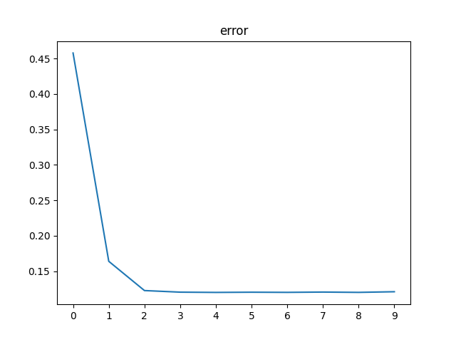
(b) $M=2\times 10^{4}$, $N=20$, time (cpu): 4096

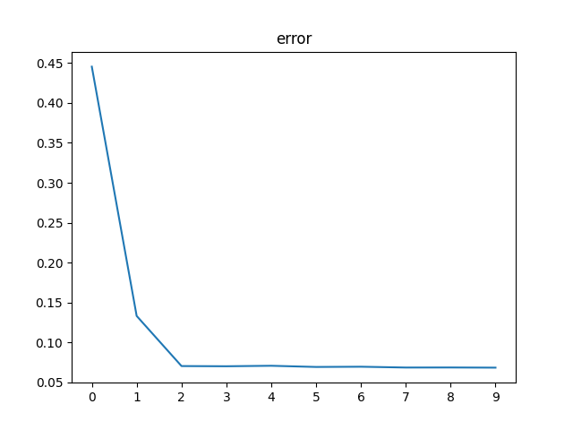
(c) $M=10^{4}$, $N=40$, time (cpu): 8409

Figure 8. Comparison of the error returned by Algorithm 2, depending on the number of particles/realizations, $\varpi=1$.

The experiments are run with the harmonic version of the fictitious play (i.e., $\varpi=1$), with: $n=10$ learning iterations, $p=30$ time steps, $\sigma=1$ and $\varepsilon=1$; 4000 units in cpu time is around 1h. The conclusion is that idiosyncratic noises demonstrate to be useful from the numerical point of view, even though the results stated in Section 2 remain the same whatever the value of $\sigma$. A careful inspection of the numerical results shows that, in fact, idiosyncratic noises provide a better fit of the solution to the Riccati equation, which is fully consistent with the conclusion of the previous paragraph. In turn, we guess that a model-based method, in which $Q$ and $R$ would be learnt first, and then the solution to the Riccati equation would be learnt separately, would make sense in this specific setting.

When $\varpi=1.1$, we observe a phenomenon similar to the one reported in Figure 7: the estimate is less accurate with the geometric version of the fictitious play. Again, we believe that this is due to the learning of the solution to the Riccati equation. In presence of a bias, the letter seems more difficult to catch. To wit, we have plotted in Figure 9, Plot (A), the error for the geometric version of the fictitious play (here, $\varpi=1.1$) and for the same parameter as in Plot (C) in Figure 8: $n=10$, $p=30$, $\sigma=1$ , $\varepsilon=1$, $M=10^{4}$ and $N=40$. In order to stress that the drawback observed on Plot (A) does not contradict our theoretical results, we have plotted in the same Figure, Plot (B), the results when the solution to the Riccati is known (which is a bit different from what is done in Figure 7 because there is here an additional idiosyncratic noise which requires additional Monte-Carlo approximations). It is clear that, in the latter case, the result is better. Possibly, this opens the door for refined procedures in which one first estimates the solution to the Riccati equation.

(a) $M=10^{4}$, $N=40$, Riccati unknown

(b) $M=10^{4}$, $N=40$, Riccati known

Figure 9. Algorithm 2, $\varpi=1.1$, depending on whether Riccati is known or not.

3.3.4. Validation

The reader could worry about a possible overfitting in our numerical experiments. Actually, in order to validate our results, we can learn the coefficients ${\bm{a}}^{n}$ and ${\bm{c}}^{n}$ in Algorithm 2 for a first series of data in (3.14). In brief, this first series of data is used to learn the equilibrium feedback. Then, we can use a second series of data (say, of the same size) in (3.14) in order to compute the error. In clear, given this second series of data, we can implement Algorithm 1 and then compute the resulting error (3.20) when $(\overline{m}_{t_{k}}^{n,(j)})_{j,k}$ and $(h_{t_{k}}^{n,(j)})_{j,k}$ therein are obtained from the formulas (3.16) and (3.18) by using the coefficients ${\bm{a}}^{n}$ and ${\bm{c}}^{n}$ returned by the first series of data and then by implementing the Euler scheme with respect to the second series of data. The resulting plots are very similar to those represented in Figure 8 (e.g., when $\varpi=1$). For this reason, we feel useless to insert them here. Intuitively, what happens is that there are sufficiently many realizations of the common noise in our experiments to guarantee, in the regression (3.15), a convenient form of averaging with respect to all these realizations.

3.4. Experiments in higher dimension

The challenge in higher dimension is twofold. The very main one is to provide an efficient regression of ${\bm{h}}^{n+1}$ onto $\overline{\bm{m}}^{n}$ (recall (3.17)). We already reported this difficulty and, as we already announced, we handle it here by using neural networks. The second issue is directly related with the computational cost. Intuitively, all the tensors that enter the code include an axis corresponding to all the possible coordinates of the noises and the states. When the dimension increases, the size of those tensors increase accordingly, which impacts the computational effort. In all the examples below, $\sigma=\varepsilon=1$. For simplicity, we just present the result in the case $\varpi=1$ because the difficulties that we report below are the same in the case $\varpi>1$.

3.4.1. Results with Algorithm 2.

In the examples below, we reduce part of the complexity by labelling the increments of the independent noises $\Delta_{t_{k}}b^{(i,j)}$ in (3.14) by the sole $i$, which allows us to save memory. We refer to Remark 3.4 for more details about this. We also limit ourselves to batches carrying $N=10^{3}$ realizations of the common noise and $M=10^{2}$ realizations of the independent noise. These numbers are a bit less than those used in the lower dimensional setting (compare for instance with Figure 8). However, differently from what we did in the previous subsection, we now use several batches. In the experiments below, the batches are indexed by an index, called batch. For a given value $i$ of this index batch, we simulate one stack, say $G_{\rm com}[i]$, of $N=10^{3}$ realizations of the common noise and then a number $m_{\rm ind}$ of sub-batches (or sub-stacks) containing, each, $M=10^{2}$ realizations of the independent noise. Those sub-batches are denoted $G_{\rm ind}[i,j]$, for $j=1,\cdots,m_{\rm ind}$. The batches contain independent realizations. In the experiments below, $m_{\rm ind}=10$.

When we start experiments with a new value $i$ of the index batch, we perform several runs of ADAM. All these runs use the same batch $G_{\rm com}[i]$ of common noises. We then repeat several times the following episode: we do a first run with the first batch $G_{\rm ind}[i,1]$ of independent noises, and then a second one with the second batch $G_{\rm ind}[i,2]$, and so on and so forth up until the batch $G_{\rm ind}[i,m_{\rm ind}]$ of index $m_{\rm ind}$. We repeat those episodes several times: 4 times in the experiments ran below. Our choice to proceed in such a way is dictated by the fact that the number $N$ is pretty low, hence the desire to have more batches for the independent noises. As for the choice $N\gg M$, it is dictated by our wish to have the lowest possible fluctuations with respect to the common noise, as the main object that we want to learn here is ${\mathfrak{h}}$ in (3.17), the input of which is measurable with respect to the common noise only. In our experiments, the index batch is running over $\{1,\cdots,20\}$. We have chosen to pass once on the realizations of the common noise.

For some choices of the matrix $\Theta$ in (3.4), our results are bad. In order to appreciate this observation, it is worth recalling that our strategy relies on a change of measure based on the Girsanov density ${\mathcal{E}}({\bm{h}}^{n})$, see (1.15). In our code, the training cost is precisely estimated under this new probability measure, as made clear in (3.15). Drawing a parallel with preferential sampling in Monte Carlo methods, one may then guess that the variance resulting from the empirical estimate of the loss in (3.15) may dramatically deteriorate as the dimension increases. Indeed, if ${\bm{h}}$ in (1.15) has all its coordinates constant equal to $1$, then

$${\mathbb{E}}\Bigl{[}{\mathcal{E}}({\bm{h}})^{2}\Bigr{]}=\exp\Bigl{(}\int_{0}^{T}|h_{s}|^{2}ds\Bigr{)}=\exp(d).$$

Even more, the fact that the control appearing in (3.15) contains a finite difference of the common noise (see (3.16) ) says that the typical size of the variance may be of order $p^{2}\exp(d)$.

In order to validate numerically this intuition, we consider the case when the matrix $(\Theta_{i,j})_{1\leq i,j\leq d}$ in (3.4) is given by $\Theta_{i,2i(\rm{mod})d}=-10$, $\Theta_{i,3i(\rm{mod})d}=10$ and $\Theta_{i,j}=0$ otherwise, where $2i(\rm{mod})d$ is the rest of the Euclidean division of $2i$ by $d$ (and similarly for $3i({\rm mod})d$). We then represent in Figure 10 the evolution of the variance of the term

$${\mathcal{E}}({\bm{h}})\int_{0}^{T}|\dot{W}_{t}^{p,{\bm{h}}}|^{2}dt,$$ (3.21)

when ${\bm{h}}$ therein is computed numerically by the FBSDE solver described in Subsection 3.2.1. We expect this term to give the worst contribution to the global variance. As shown by the plot in Figure 10, the log variance becomes higher at multiples of 6 (because of the choice $\Theta$) and the plot even suggests that the variance could blow up exponentially fast along the subsequence 6, 12, 18, 24…

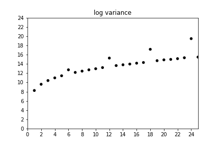
Figure 10. Evolution of the log variance of the loss with the dimension for $\Theta_{i,2i(\rm{mod})d}=-10$, $\Theta_{i,3i(\rm{mod})d}=10$ in (3.4). Dimension is in $x$-axis. Log variance is in $y$-axis.

We thus chose to run Algorithm 2 with $d=12$ with aforementioned values of $M$ and $N$ and with $p=20$ time steps. The results are reported in Figure 11 below.

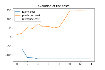
(a) Evolution of the costs

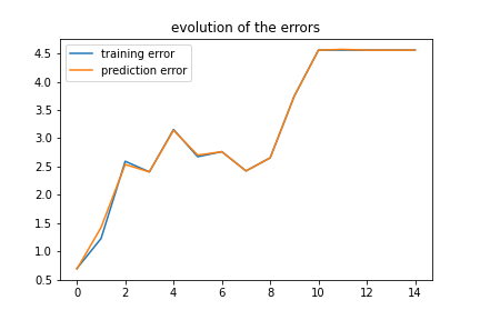
(b) Evolution of the errors

Figure 11. Results in dimension $d=12$ for $\Theta_{i,2i(\rm{mod})d}=-10$, $\Theta_{i,3i(\rm{mod})d}=10$ in (3.4). Harmonic variant of the fictitious play ($\varpi=1$).

We clearly observe that the learnt cost blows-up. Subsequently, the training error does not vanish, with the training error being here computed as in (3.20) but solely for the ${\bm{h}}$ part, that is

$$\biggl{[}\frac{1}{Np}\sum_{j=1}^{N}\sum_{k=0}^{p-1}|h_{t_{k}}^{(j)}-h_{t_{k}}^{\star,(j)}|^{2}\biggr{]}^{1/2}.$$ (3.22)

In the plot, we also include a prediction cost and a prediction error, which are computed on a batch different from the batches used for training (but of the same size). Given a new batch for the common and independent noises, we can indeed use the neural network returned by the training phase to compute, for this new batch, a prediction of the cost (together with a prediction of ${\bm{h}}$), but under the historical probability measure ${\mathbb{P}}$ (in order to avoid any variance issues). The prediction is thus constructed as follows. Given the returns $(a_{t_{k}})_{k=0,\cdots,p-1}$ and $({\mathfrak{h}}_{t_{k}})_{k=0,\cdots,p-1}$ of the neural network for the affine feedback, see (3.13) and (3.17), we implement the following Euler scheme:

$$\begin{split}&x_{t_{k}}^{(i,j)}=x_{t_{k-1}}^{(i,j)}+\frac{1}{p}\alpha_{t_{k}}^{(i,j)}+{\frac{1}{\sqrt{p}}}\Delta_{t_{k}}b^{(i)}+{\frac{1}{\sqrt{p}}}\Delta_{t_{k}}w^{(j)},\quad\ell=1,\cdots,p\ ;\quad x_{0}^{(i,j)}=x_{0},\\ &\alpha_{t_{k}}^{(i,j)}=a_{t_{k-1}}x_{t_{k-1}}^{(i,j)}+{\mathfrak{h}}_{t_{k-1}}(\overline{m}_{t_{k-1}}^{(j)}),\quad k=1,\cdots,p,\end{split}$$

with $\overline{m}_{t_{k-1}}^{(j)}=M^{-1}\sum_{i=1}^{M}x_{t_{k-1}}^{(i,j)}$.

The predicted cost is then

$$\frac{1}{N}\sum_{j=1}^{N}\frac{1}{M}\sum_{i=1}^{M}\biggl{[}\frac{1}{2p}\sum_{k=1}^{p}|\alpha_{t_{k}}^{(i,j)}|^{2}+\frac{1}{2}\Bigl{|}x^{(i,j)}_{1}+g\Bigl{(}\overline{m}_{1}^{n,(j)}\Bigr{)}\Bigr{|}^{2}\biggr{]},$$

and the predicted error is (3.22).

While their role is rather limited at this stage, the two prediction cost and error play a more important role in the next paragraph.

3.4.2. Variance reduction.

The issue reported in the previous paragraph calls for the implementation of a variance reduction method. The method that is addressed in this new paragraph aims at reducing the variance associated with the dominant term (3.21). The key point is to return back to (2.30), to write the normalization factor $-d\,\varepsilon^{2}p/2$ as the expectation

$$\varepsilon{\mathbb{E}}^{{\bm{h}}_{n}}\int_{0}^{T}\alpha_{t}\dot{W}_{t}^{p,{\bm{h}}^{n}}dt-\frac{\varepsilon^{2}}{2}{\mathbb{E}}^{{\bm{h}}_{n}}\int_{0}^{T}\bigl{|}\dot{W}_{t}^{p,{\bm{h}}^{n}}\bigr{|}^{2}dt,$$ (3.23)

which is indeed equal to $-d\,\varepsilon^{2}p/2$, and then to approximate the above two expectations by two empirical means. Intuitively (and this is the computation achieved in (2.30)), the resulting estimator of the cost coincides with the estimator that would be computed if we had to solve (the reader may compare the following cost with (2.32), with $\varpi=1$ for simplicty)

$$\textrm{\rm argmin}_{\bm{\alpha}}{\mathbb{E}}^{{\bm{h}}^{n}}\bigl{[}{\mathcal{R}}^{p}\bigl{(}{\bm{\alpha}};\overline{\bm{m}}^{n};\varepsilon{\bm{W}}^{p}\ \bigr{)}\bigr{]},$$ (3.24)

which is implicitly set over the dynamics

$$\mathrm{d}X_{t}=\alpha_{t}\mathrm{d}t+\sigma\mathrm{d}B_{t}+\varepsilon\mathrm{d}W_{t}^{p,{\bm{h}}^{n}},\quad t\in[0,T].$$ (3.25)

Here, we have two formulations depending on the line that is used in (2.32): $(i)$ We have the formulation (3.24)–(3.25), which is based on the second line in (2.32); $(ii)$ And we have the formulation based on the top line in (2.32) when the corrector $-d\,\varepsilon^{2}p/2$ therein is replaced by the empirical mean deriving from (3.23). Interestingly, the two formulations do not have the same practical interpretation. Indeed, the formulation $(i)$ does not fit the principle of Figure 2 in introduction since the common randomization therein does not impact the control directly, but impacts the dynamics. Differently, the formulation $(ii)$ based on the empirical corrector associated with (3.23) preserves the principle of Figure 2 since the corrector can be computed separately from the control. Of course, it has a practical price: implicitly, computing the correction empirically makes sense only if the dependence of the running cost upon the control is known. In other words, part of the model must be known.

Figure 12 below provides an estimate of the variance of the (random) cost in (3.24) when ${\bm{h}}^{n}$ is replaced by the numerical solution ${\bm{h}}$ of the FBSDE solver described in Subsection 3.2.1 and when $\Theta$ is computed as in Figure 10. As the reader can notice, the growth is slower (than in Figure 10).

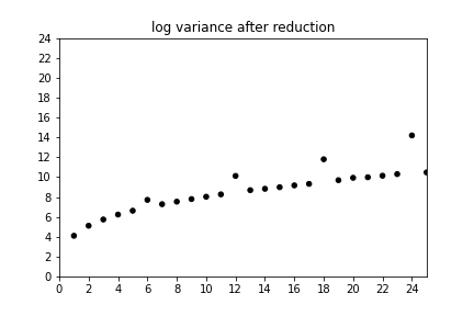
Figure 12. Evolution of the log variance of the corrected optimal cost (3.24). with the dimension for $\Theta_{i,2i(\rm{mod})d}=-10$, $\Theta_{i,3i(\rm{mod})d}=10$ in (3.4). Dimension is in $x$-axis. Log variance is in $y$-axis. Harmonic variant of the fictitious play ($\varpi=1$).

The estimator for (3.23) writes as in (3.15), namely

$$\begin{split}&\frac{\varepsilon}{N}\sum_{j=1}^{N}\biggl{(}{\mathcal{E}}^{n,(j)}\frac{1}{M}\sum_{i=1}^{M}\biggl{[}\frac{1}{2p}\sum_{k=1}^{p}\alpha_{t_{k}}^{(i,j)}\cdot\Bigl{(}h^{n,(j)}_{t_{k}}+p\Delta_{t_{k+1}}w^{(j)}\Bigr{)}\biggr{]}\biggr{)}\\ &\hskip 15.0pt-\frac{\varepsilon^{2}}{2N}\sum_{j=1}^{N}\biggl{(}{\mathcal{E}}^{n,(j)}\frac{1}{2p}\sum_{k=1}^{p}\Bigl{|}h^{n,(j)}_{t_{k}}+p\Delta_{t_{k+1}}w^{(j)}\Bigr{|}^{2}\biggr{)}.\end{split}$$

The results are represented in Figure 13 for the same choice of $d$ and $\Theta$ as in Figure 11. Obviously, they are much more convincing than in Figure 7. On the left pane (A), the reference cost is computed by solving first the FBSDE described in Subsection 3.2.1 on a series of batches and then by averaging the corresponding costs over the batches. In contrast, the empirical cost is computed by solving the FBSDE and the associated cost on the batch on which the training loss is computed. The fact that the reference and empirical costs do not coincide shows that there is, in between, some additional Monte-Carlo error that is distinct from the learning procedure.

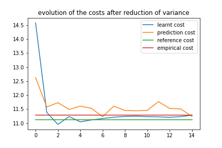
(a) Evolution of the losses

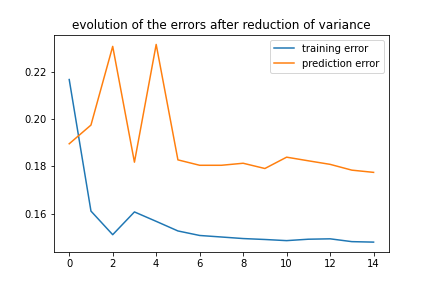
(b) Evolution of the errors

Figure 13. Results in dimension $d=12$ for $\Theta_{i,2i(\rm{mod})d}=-10$, $\Theta_{i,3i(\rm{mod})d}=10$ in (3.4). Harmonic variant of the fictitious play ($\varpi=1$).

The prediction cost and error are computed on a series of 10 batches (of the same size as before). The cost and the error that are plotted are obtained by averaging out on the batches. We observe a small bias between the training and prediction errors that would deserve further experiments. Anyway the main message is clear: the plots after variance reduction are much better than before variance reduction.

We now provide another example, with a new choice of $\Theta$, that exhibits a less trivial evolution of the prediction error. Namely, we choose $\Theta=(\theta_{i,j}=(i+j)/(2d))_{i,j}$. The results in Figure 14 may be summarized as follows: the relative error on the cost is less than $0.03$ and the prediction error is less than $0.2$. As for the latter, it must be recalled that the prediction error writes as a $d$-dimensional norm, see (3.22). In particular, the mean square error per coordinate is less than $0.2^{2}/d$. Here, $d=12$ and the mean error per coordinate is less than $0.06$. We address the same example in Figure 15 in dimension $d=20$. The absolute error on the cost is good, except at iterations 11 and 13, but even for these two the relative error is less than $0.05$. The prediction error is between $0.22$ and $0.25$ after iteration 6, except at iterations 11 and 13, where the prediction error reaches 0.32. In any case, the mean error per coordinate is less than $0.07$ after iteration 6.

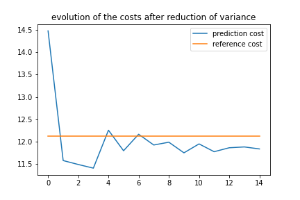
(a) Evolution of the losses

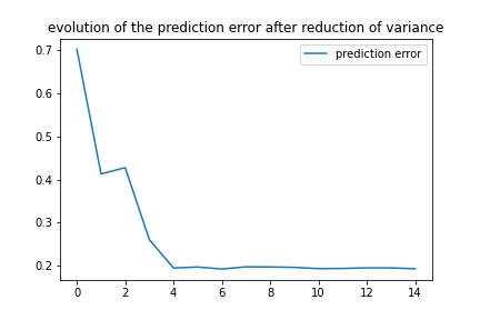
(b) Evolution of the errors

Figure 14. Results in dimension $d=12$ for $\Theta=(\theta_{i,j}=(i+j)/(2d))_{i,j}$ in (3.4). The reference loss is around 12.17 and the prediction loss at iteration 14 is 11.84. The prediction error at iteration 14 is around 0.19. Harmonic variant of the fictitious play ($\varpi=1$).

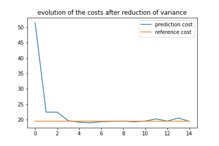
(a) Evolution of the losses

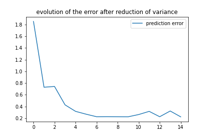
(b) Evolution of the errors

Figure 15. Results in dimension $d=20$ for $\Theta=(\theta_{i,j}=(i+j)/(2d))_{i,j}$ in (3.4). The reference loss is around 19.47 and the prediction loss at iteration 14 is 19.45. The prediction error at iteration 14 is around 0.22. Harmonic variant of the fictitious play ($\varpi=1$).

3.5. Small viscosity

The next question in our numerical experiments is to address the behavior of the algorithm as the viscosity tends to $0$. As made clear in the analysis performed in Section 2, the influence of the small viscosity may manifest in an exponential manner and this was our original motivation to design a geometrically converging scheme.

Beyond the theoretical challenge raised by the possible occurrence of singularities in the vanishing viscosity limit (an example of which is given by Lemma 2.8), small viscosity may also create additional numerical instability phenomena. As a main example, high variances may occur in the computations of empirical measures under the tilted probability measure. Obviously, this follows from the fact that the Girsanov density driving the change of reference measure in the algorithm becomes highly singular as the viscosity tends to $0$. We reported a similar drawback in the previous subsection, but in the large dimensional framework. In the first arXiv version [34] of this work, the observation of this phenomenon prompted us to introduce a method at the intersection between annealed simulating and preferential sampling, which we illustrated on a specific example that is recalled below. While this method is performing well (we revisit it in the framework of the geometric fictitious play in this subsection), it requires to repeat the scheme for several values of the viscosity and it is thus rather costly.

Instead, we here show that the geometric fictitious play can quickly return a very accurate numerical solution to the vanishing viscosity property problem (at least in the example addressed in the first arXiv version [34]). This is a very striking exemplification of our approach. It clearly demonstrates the benefits of choosing a higher value of the rate $\varpi$ and therefore of working with the geometric variant (instead of the harmonic variant) of the fictitious play. Our numerical experiment based on the aforementioned benchmark model. We choose a variant of $g$ in (3.2), with $d=1$:

$$g(x)=\cos\bigl{(}\kappa(x-x_{0})\bigr{)}-2x_{0},$$ (3.26)

with $\kappa=10$ and where $x_{0}$ is a root of the equation

$$\cos\bigl{(}\kappa x_{0}\bigr{)}=2x_{0}.$$

Numerically, we find that a choice is $x_{0}\approx-0.384$. The motivation for such an $x_{0}$ is that $0$ is a solution of (3.9). In other words, $0$ is an equilibrium. Even more, we observe that, if the viscosity is zero, then the iterative sequence defined through the two updating rules (1.9) and (1.10) remains in $({\bm{m}}^{n},{\bm{h}}^{n})=(0,-2x_{0})$ for any $n\geq 1$ if ${\bm{m}}^{0}$ is chosen as $0$. In other words, the standard fictitious (without any exploration) play converges (as predicted by the theory since this 1-dimensional MFG is potential, see §3.1.2) and chooses the $0$-equilibrium. In order to compare with the prediction method exposed in §3.1.2, we have plotted the corresponding potential (which is given by a primitive $G$ of $g$). The plots are given in Figure 16. We observe that $0$ is just a local minimizer of the potential and that the global minimizer is around $-0.5$.

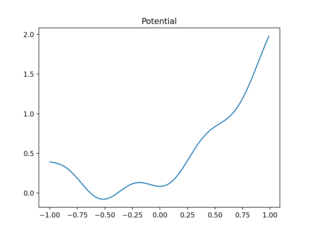
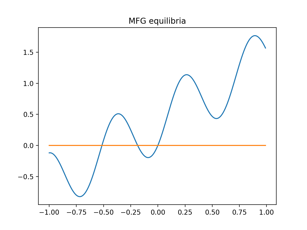
Figure 16. Equilibrium predicted by the potential rule: Potential $G$ on the left pane; Zeros of the function $g$ in the right pane.

Our geometric fictitious play is able to rule out the $0$-equilibrium and to retain the other one. In order to check this numerically, we have used three values for $\varpi$: $\varpi=4$, $\varpi=1.5$ and $\varpi=1$. As for the other parameters, we have chosen $\sigma=0$ (no idiosyncratic noise, but Riccati is known), $M=2\times 10^{4}$ (number of Monte-Carlo simulations) and $p=100$. In all the experiments, $\varepsilon$ is set equal to $0.2$. The algorithm is initialized from the local minimizer. Our regression on the Hermite polynomials goes up to polynomials of degree 6. The results are presented in Figures 17, 18 and 19. Therein, we have plotted the histogram, under the tilted probability measure and at the end of each episode, of the terminal conditional mean of the system. Even though the regime $\varpi=4$ is outside the scope of Theorem 2.4 (because we assumed $\varpi\in(1,\sqrt{2}]$), the result with this choice is quite impressive: the right equilibrium is selected in five iterations only. When $\varpi=1.5$, ten iterations are necessary. When $\varpi=1$, the results are satisfactory with around fifteen iterations but it is clear that the histogram features a kind of residual variance, which makes the selection less obvious. We believe that these plots are a strong case for supporting our results.

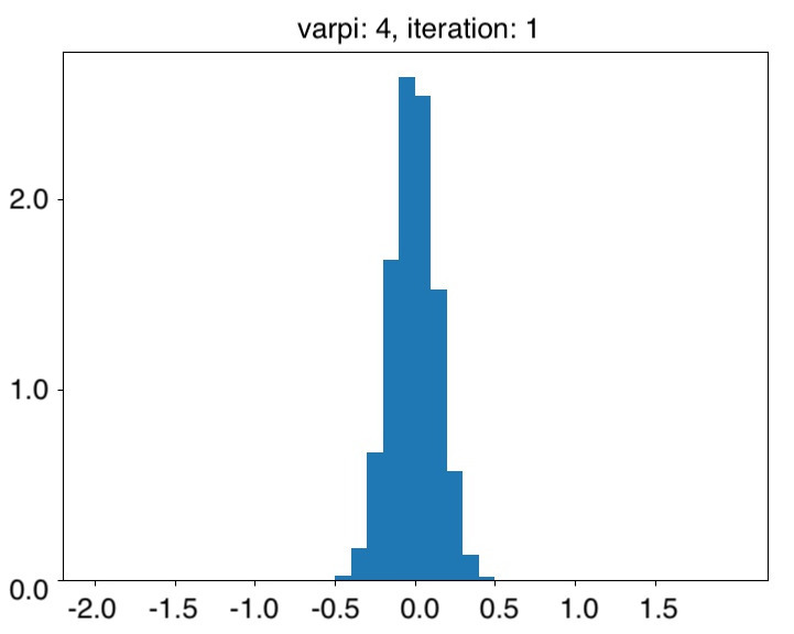
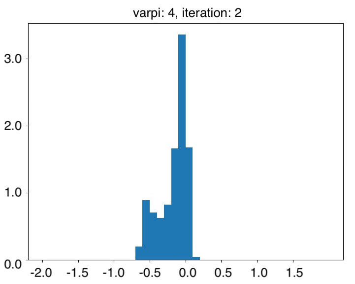
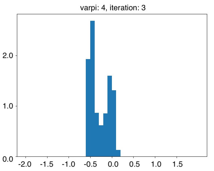
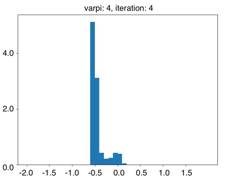
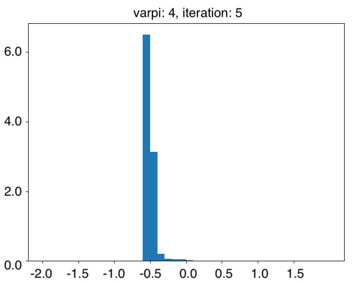
Figure 17. Selection of a solution by vanishing viscosity: histogram under the tilted measure of the terminal mean for $\varepsilon=0.2$ and $\varpi=4$. Equilibrium is clearly selected in 5 iterations.

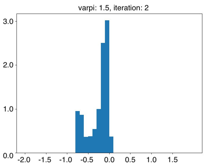
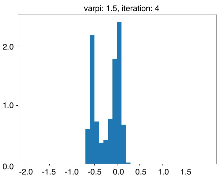
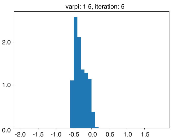
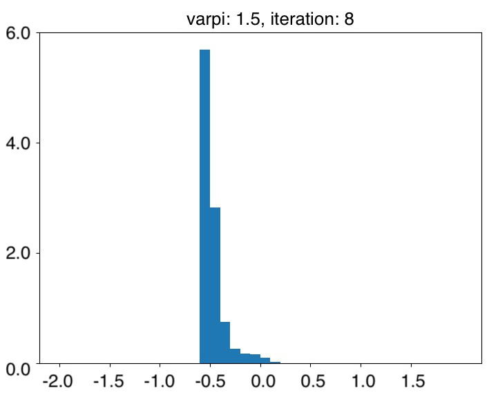
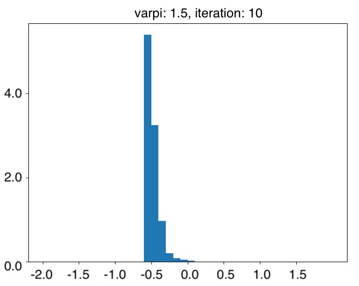
Figure 18. Selection of a solution by vanishing viscosity: histogram under the tilted measure of the terminal mean for $\varepsilon=0.2$ and $\varpi=1.5$. Equilibrium is selected in 10 iterations.

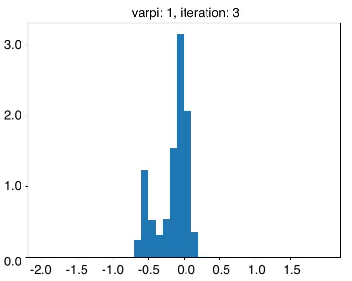
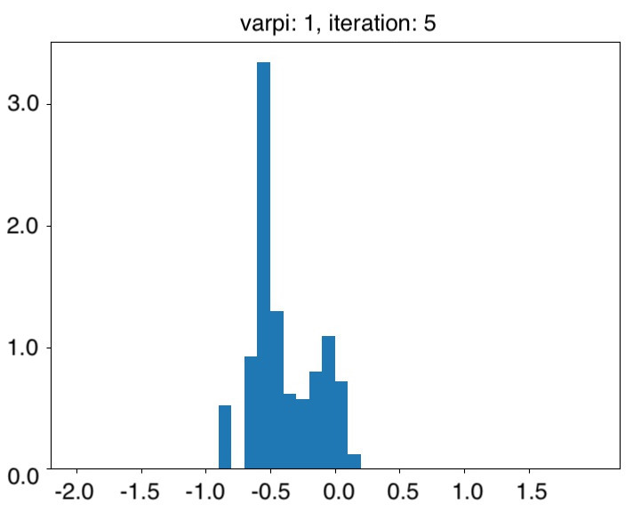
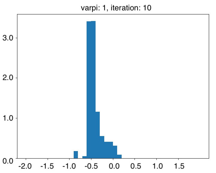
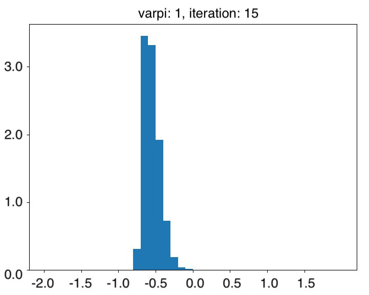
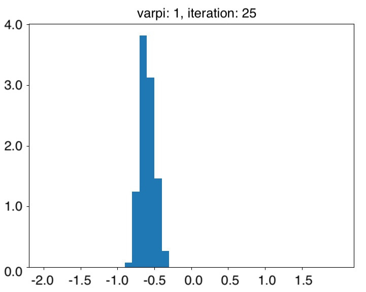
Figure 19. Selection of a solution by vanishing viscosity: histogram under the tilted measure of the terminal mean for $\varepsilon=0.2$ and $\varpi=1$. Equilibrium is selected in more than 10 iterations, with a non-trivial residual variance.

For sure, the reader may wonder about the same plots if we decrease the value of $\varepsilon$ (say $\varepsilon=0.1$). It is fair to recognize that the results are not so good when $\varepsilon=0.1$. To our mind, this is due to the variance issues that we reported above: the Girsanov change of reference may induce high variances. Numerical observations seem to indicate that those issues may even get worse when increasing the value of $\varpi$ (which is not so easy to explain from a theoretical point of view because the integrand $\varpi{\bm{h}}^{n}$ in (2.1) is close to the true solution ${\bm{h}}$, regardless of the value of $\varpi$). One possible strategy to reduce the underlying variance would be to implement the same preferential sampling argument as in the first arXiv version [34], but it is fair to say that it is difficult to obtain a plot that is as good as the one obtained in Figure 17. For this reason, we feel better to address this possible extension in a future work.

References

- [1] Y. Achdou, F. Camilli, and I. Capuzzo-Dolcetta. Mean field games: numerical methods for the planning problem. SIAM J. Control Optim., 50(1):77–109, 2012.
- [2] Y. Achdou, F. Camilli, and I. Capuzzo-Dolcetta. Mean field games: convergence of a finite difference method. SIAM J. Numer. Anal., 51(5):2585–2612, 2013.
- [3] Y. Achdou and I. Capuzzo-Dolcetta. Mean field games: numerical methods. SIAM J. Numer. Anal., 48(3):1136–1162, 2010.
- [4] Y. Achdou and M. Laurière. Mean field type control with congestion (II): An augmented Lagrangian method. Appl. Math. Optim., 74(3):535–578, 2016.
- [5] Y. Achdou and M. Laurière. Mean field games and applications: Numerical aspects. In Mean Field Games, Cetraro, Italy 2019, Cardaliaguet, Pierre, Porretta, Alessio (Eds.), LNM 2281, pages 203–248. Springer, 2021.
- [6] C. Alasseur, I. Ben Taher, and A. Matoussi. An extended mean field game for storage in smart grids. J. Optim. Theory Appl., 184(2):644–670, 2020.
- [7] E. Bayraktar, A. Cecchin, A. Cohen, and F. Delarue. Finite state mean field games with Wright-Fisher common noise. J. Math. Pures Appl., 147:98–162, 2021.
- [8] C. Beck, W. E, and A. Jentzen. Machine learning approximation algorithms for high-dimensional fully nonlinear partial differential equations and second-order backward stochastic differential equations. J. Nonlinear Sci., 29(4):1563–1619, 2019.
- [9] J.-D. Benamou and G. Carlier. Augmented Lagrangian methods for transport optimization, mean field games and degenerate elliptic equations. J. Optim. Theory Appl., 167(1):1–26, 2015.
- [10] C. Bender and J. Zhang. Time discretization and Markovian iteration for coupled FBSDEs. Ann. Appl. Probab., 18(1):143–177, 2008.
- [11] P. Briand and C. Labart. Simulation of BSDEs by Wiener chaos expansion. Ann. Appl. Probab., 24(3):1129–1171, 2014.
- [12] L. Briceño Arias, D. Kalise, Z. Kobeissi, M. Laurière, A. Mateos González, and F. J. Silva. On the implementation of a primal-dual algorithm for second order time-dependent mean field games with local couplings. In CEMRACS 2017—numerical methods for stochastic models: control, uncertainty quantification, mean-field, volume 65 of ESAIM Proc. Surveys, pages 330–348. EDP Sci., Les Ulis, 2019.
- [13] L. M. Briceño Arias, D. Kalise, and F. J. Silva. Proximal methods for stationary mean field games with local couplings. SIAM J. Control Optim., 56(2):801–836, 2018.
- [14] P. Cardaliaguet and S. Hadikhanloo. Learning in mean field games: the fictitious play. ESAIM Control Optim. Calc. Var., 23(2):569–591, 2017.
- [15] E. Carlini and F. J. Silva. A fully discrete semi-Lagrangian scheme for a first order mean field game problem. SIAM J. Numer. Anal., 52(1):45–67, 2014.
- [16] E. Carlini and F. J. Silva. A semi-Lagrangian scheme for a degenerate second order mean field game system. Discrete Contin. Dyn. Syst., 35(9):4269–4292, 2015.
- [17] R. Carmona and F. Delarue. Probabilistic theory of mean field games with applications. I, volume 83 of Probability Theory and Stochastic Modelling. Springer, Cham, 2018. Mean field FBSDEs, control, and games.
- [18] R. Carmona and F. Delarue. Probabilistic theory of mean field games with applications. II, volume 84 of Probability Theory and Stochastic Modelling. Springer, Cham, 2018. Mean field games with common noise and master equations.
- [19] R. Carmona and D. Lacker. A probabilistic weak formulation of mean field games and applications. Ann. Appl. Probab., 25(3):1189–1231, 2015.
- [20] R. Carmona and M. Laurière. Convergence analysis of machine learning algorithms for the numerical solution of mean field control and games I: The ergodic case. SIAM J. Numer. Anal., 59(3):1455–1485, 2021.
- [21] R. Carmona, M. Laurière, and Z. Tan. Linear-quadratic mean-field reinforcement learning: convergence of policy gradient methods. arXiv e-prints, arXiv:1910.04295, 2019.
- [22] R. Carmona, M. Laurière, and Z. Tan. Model-free mean field reinforcement learning: mean field MDP and mean-field Q-learning. arXiv e-prints, arXiv:1910.12802, 2019.
- [23] R. Carmona and M. Laurière. Convergence analysis of machine learning algorithms for the numerical solution of mean field control and games: II—The finite horizon case. Ann. Appl. Probab., 32(6):4065–4105, 2022.
- [24] A. Cecchin and F. Delarue. Selection by vanishing common noise for potential finite state mean field games. Comm. Partial Differential Equations, 47(1):89–168, 2022.
- [25] J.-F. Chassagneux, D. Crisan, and F. Delarue. Numerical method for FBSDEs of McKean-Vlasov type. Ann. Appl. Probab., 29(3):1640–1684, 2019.
- [26] P. E. Chaudru de Raynal and C. A. Garcia Trillos. A cubature based algorithm to solve decoupled McKean-Vlasov forward-backward stochastic differential equations. Stochastic Process. Appl., 125(6):2206–2255, 2015.
- [27] D. Crisan and E. McMurray. Cubature on Wiener space for McKean-Vlasov SDEs with smooth scalar interaction. Ann. Appl. Probab., 29(1):130–177, 2019.
- [28] J. Cvitanić and J. Zhang. The steepest descent method for forward-backward SDEs. Electron. J. Probab., 10:1468–1495, 2005.
- [29] F. Delarue. On the existence and uniqueness of solutions to FBSDEs in a non-degenerate case. Stochastic Processes and their Applications, 99(2):209 – 286, 2002.
- [30] F. Delarue. Estimates of the solutions of a system of quasi-linear PDEs. A probabilistic scheme. In Séminaire de Probabilités XXXVII, volume 1832 of Lecture Notes in Math., pages 290–332. Springer, Berlin, 2003.
- [31] F. Delarue. Restoring uniqueness to mean-field games by randomizing the equilibria. Stochastics and Partial Differential Equations: Analysis and Computations, 7:598–678, 2019.
- [32] F. Delarue and R. Foguen Tchuendom. Selection of equilibria in a linear quadratic mean field game. Stochastic Processes and their Applications, 130(2):1000–1040, 2020.
- [33] F. Delarue and S. Menozzi. A forward-backward stochastic algorithm for quasi-linear PDEs. Ann. Appl. Probab., 16(1):140–184, 2006.
- [34] F. Delarue and A. Vasileiadis. Exploration noise for learning linear-quadratic mean field games. arXiv e-prints, arXiv:2107.00839, v1, 2021.
- [35] P. Dorato and A. Levis. Optimal linear regulators: The discrete-time case. IEEE Transactions on Automatic Control, 16:613–620, 1971.
- [36] K. Doya. Reinforcement learning in continuous time and space. Neural Comput., 12(1):219–245, 2000.
- [37] W. E, J. Han, and A. Jentzen. Deep learning-based numerical methods for high-dimensional parabolic partial differential equations and backward stochastic differential equations. Commun. Math. Stat., 5(4):349–380, 2017.
- [38] R. Elie, L. Pérolat, M. Laurière, M. Geist, and O. Pietquin. On the convergence of model free learning in mean field games. AAAI, 2020.
- [39] D. Firoozi and S. Jaimungal. Exploratory LQG mean field games with entropy regularization. Automatica, 139:110177, 2022.
- [40] R. Foguen Tchuendom. Uniqueness for linear-quadratic mean field games with common noise. Dyn. Games Appl., 8(1):199–210, 2018.
- [41] M. Geist, J. Pérolat, M. Laurière, R. Elie, S. Perrin, O. Bachem, R. Munos, and O. Pietquin. Concave utility reinforcement learning: The mean-field game viewpoint. In P. Faliszewski, V. Mascardi, C. Pelachaud, and M. E. Taylor, editors, 21st International Conference on Autonomous Agents and Multiagent Systems, AAMAS 2022, Auckland, New Zealand, May 9-13, 2022, pages 489–497. International Foundation for Autonomous Agents and Multiagent Systems (IFAAMAS), 2022.
- [42] E. Gobet, J.-P. Lemor, and X. Warin. A regression-based Monte Carlo method to solve backward stochastic differential equations. Ann. Appl. Probab., 15(3):2172–2202, 2005.
- [43] X. Guo, A. Hu, R. Xu, and J. Zhang. Learning mean-field games. In Proceedings of NeurIPS. 2019.
- [44] S. Hadikhanloo. Learning in anonymous nonatomic games with applications to first-order mean field games. arXiv e-prints, arXiv:1704.00378, 2017.
- [45] S. Hadikhanloo and F. J. Silva. Finite mean field games: fictitious play and convergence to a first order continuous mean field game. J. Math. Pures Appl. (9), 132:369–397, 2019.
- [46] B. Hambly, R. Xu, and H. Yang. Policy gradient methods find the Nash equilibrium in N-player general-sum linear-quadratic games. J. Mach. Learn. Res., 24:Paper No. [139], 56, 2023.
- [47] R. Hu and M. Laurière. Recent Developments in Machine Learning Methods for Stochastic Control and Games. HAL archives, hal-03656245, May 2022. working paper or preprint.
- [48] K. Huang, X. Di, Q. Du, and X. Chen. A game-theoretic framework for autonomous vehicles velocity control: bridging microscopic differential games and macroscopic mean field games. Discrete Contin. Dyn. Syst. Ser. B, 25(12):4869–4903, 2020.
- [49] M. Huang, P. Caines, and R. Malhamé. Individual and mass behavior in large population stochastic wireless power control problems: centralized and Nash equilibrium solutions. pages 98 – 103, 2003.
- [50] M. Huang, P. E. Caines, and R. P. Malhamé. The Nash certainty equivalence principle and McKean-Vlasov systems: An invariance principle and entry adaptation. In Decision and Control, 2007 46th IEEE Conference on, pages 121–126. IEEE, 2007.
- [51] M. Huang, R. P. Malhamé, and P. E. Caines. Large population stochastic dynamic games: Closed-loop McKean-Vlasov systems and the Nash certainty equivalence principle. Commun. Inf. Syst., 6(3):221–251, 2006.
- [52] T. P. Huijskens, M. J. Ruijter, and C. W. Oosterlee. Efficient numerical Fourier methods for coupled forward-backward SDEs. J. Comput. Appl. Math., 296:593–612, 2016.
- [53] J. Jacod and P. Protter. Probability essentials. Universitext. Springer-Verlag, Berlin, second edition, 2003.
- [54] N. Kazamaki. Continuous exponential martingales and BMO, volume 1579 of Lecture Notes in Mathematics. Springer-Verlag, Berlin, 1994.
- [55] J.-M. Lasry and P.-L. Lions. Jeux à champ moyen. I. Le cas stationnaire. C. R. Math. Acad. Sci. Paris, 343(9):619–625, 2006.
- [56] J.-M. Lasry and P.-L. Lions. Jeux à champ moyen. II. Horizon fini et contrôle optimal. C. R. Math. Acad. Sci. Paris, 343(10):679–684, 2006.
- [57] J.-M. Lasry and P.-L. Lions. Mean field games. Jpn. J. Math., 2(1):229–260, 2007.
- [58] P.-L. Lions. Cours au Collège de France, Equations aux dérivées partielles et applications. https://www.college-de-france.fr/site/pierre-louis-lions/course.htm.
- [59] J. Ma, P. Protter, and J. Yong. Solving forward-backward stochastic differential equations explicitly – a four step scheme. Probability Theory and Related Fields, 98(3):339–359, 1994.
- [60] J. Ma, J. Shen, and Y. Zhao. On numerical approximations of forward-backward stochastic differential equations. SIAM J. Numer. Anal., 46(5):2636–2661, 2008.
- [61] G. N. Milstein and M. V. Tretyakov. Numerical algorithms for semilinear parabolic equations with small parameter based on approximation of stochastic equations. Math. Comp., 69(229):237–267, 2000.
- [62] P. Muller, M. Rowland, R. Elie, G. Piliouras, J. Perolat, M. Lauriere, R. Marinier, O. Pietquin, and K. Tuyls. Learning equilibria in mean-field games: Introducing mean-field PSRO. In AAMAS ’22: Proceedings of the 21st International Conference on Autonomous Agents and Multiagent Systems, page Pages 926–934, 2022.
- [63] R. Munos. A study of reinforcement learning in the continuous case by the means of viscosity solutions. Machine Learning, 40:265–299, 2000.
- [64] R. Murray and M. Palladino. A model for system uncertainty in reinforcement learning. Systems & Control Letters, 122:24–31, 2018.
- [65] S. Perrin, M. Laurière, J. Pérolat, M. Geist, R. Élie, and O. Pietquin. Mean Field Games Flock! The Reinforcement Learning Way. In Proc. of IJCAI 2021, 2021.
- [66] S. Perrin, J. Pérolat, M. Laurière, M. Geist, R. Elie, and O. Pietquin. Fictitious play for mean field games: Continuous time analysis and applications. Thirty-fourth Conference on Neural Information Processing Systems (NeurIPS 2020), December 2020.
- [67] R. S. Sutton and A. G. Barto. Reinforcement learning: an introduction. Adaptive Computation and Machine Learning. MIT Press, Cambridge, MA, second edition, 2018.
- [68] H. Wang, T. Zariphopoulou, and X. Y. Zhou. Reinforcement learning in continuous time and space: A stochastic control approach. Journal of Machine Learning Research, 21(198):1–34, 2020.
- [69] T. Z. Xin Guo, Renyuan Xu. Entropy Regularization for Mean Field Games with Learning. arXiv:2010.00145, 2020.
- [70] J. Yong and X. Y. Zhou. Stochastic controls, volume 43 of Applications of Mathematics (New York). Springer-Verlag, New York, 1999. Hamiltonian systems and HJB equations.