Technical Report

Abstract

We present a methodology for systematically extending epidemic models to multilevel and multiscale spatio-temporal pandemic ones. Our approach builds on the use of coloured stochastic and continuous Petri nets facilitating the sound component-based extension of basic SIR models to include population stratification and also spatio-geographic information and travel connections, represented as graphs, resulting in robust stratified pandemic metapopulation models. This method is inherently easy to use, producing scalable and reusable models with a high degree of clarity and accessibility which can be read either in a deterministic or stochastic paradigm. Our method is supported by a publicly available platform PetriNuts; it enables the visual construction and editing of models; deterministic, stochastic and hybrid simulation as well as structural and behavioural analysis. All the models are available as supplementary material, ensuring reproducibility.

cite as

@techreport{CGH21.report,
  author = {S Connolly and D Gilbert and M Heiner},
  title = {{From Epidemic to Pandemic Modelling}},
  institution = {Brunel University London /
                 Brandenburg University of Technology Cottbus-Senftenberg},
  year = {2021},
  month = {30 March},
  note = {Technical Report},
  pdf = {},
  url = {},
}

1 Introduction

We present a methodology for modelling pandemics, the development of which was motivated by the current COVID19 outbreak. The key point of our approach is the introduction of geography and travel connections in a well founded manner, facilitating intuitive understanding by modellers, clinicians, epidemiologists, public health strategists, politicians, and other key stakeholders.

Our modelling approach builds on the use of coloured stochastic and continuous Petri nets which facilitates the sound component-based extension of basic SIR models to include population stratification and also spatio-geographic information, resulting in robust stratified pandemic metapopulation models. This method is inherently easy to use, producing scalable and reusable models with a high degree of clarity and accessibility which can be read either in a stochastic or deterministic paradigm, the latter mapping to Ordinary Differential Equations (ODEs). The ODEs are uniquely defined by the Petri net models and are automatically generated by our simulators. In turn this conforms with sound model engineering practice, with the aim of minimising encoding errors.

The models which we obtain by our method are multilevel, the lower level comprising homogeneous SIR models, and the upper level being a network of geographical connections. Thus our methodology enables the construction and analysis of metapopulation models. The models are multiscale in terms of distances, which are explicit at the upper geographical level and implicit at the lower homogeneous level, and multiscale in terms of time in that we assume that geographical connections (travel) occur at a much lower rate than infections in lower level SIR components.

Our method is supported by a publicly available platform PetriNuts which enables visual construction and editing of models; deterministic, stochastic and hybrid simulation as well as structural and behavioural analysis. All the models presented in this paper are provided as Supplementary Material, and can be processed using the platform, thus ensuring reproducibility.

2 Results

2.1 Basic epidemic SIR model in Petri nets

We start off with the standard SIR epidemic model and the usual assumptions (see Methods section); its Petri net representation is given in Figure 1.

The infection rate is effectively the observed increase in the number of daily infections, more generally the number of infections in a given time period, typically described by mass action kinetics [WW45]. An alternative approach, called the standard incidence, normalises the infection rate by the total population size $N$, based on the assumption that daily encounters between individuals in the population are largely independent of community size [Het00]. The rate constant of infection $k_{infect}$ (the parameter for mass action kinetics) is driven by both the infectiousness of the disease, as well as any societal prevention measure in place (isolation etc.). Likewise, the recovery rate is governed by the rate constant of recovery $k_{recover}$ which reflects the contribution of all the factors contributing to recovery - health of the individuals in the population, treatment etc.

These infection and recovery rates correspond to the rate functions associated with the transitions Infect and Recover in the Petri net model. Rate functions can be interpreted in two different ways: stochastic or deterministic, thus yielding stochastic Petri nets ($\mathcal{SPN}$) or continuous Petri nets ($\mathcal{CPN}$). The semantics of $\mathcal{SPN}$ is given by continuous time Markov chains (CTMC), and the semantics of $\mathcal{CPN}$ by Ordinary Differential Equations (ODEs). The ODEs generated reading the Petri net in Figure 1 as a $\mathcal{CPN}$ are given in Equation 1, which correspond exactly to the ODEs given in the literature. We observe that each place gets its own equation (see Methods section for the automatic translation of $\mathcal{CPN}$ into ODEs). In the equations we have replaced the long place names by their standard short forms for readability. The formulae governing the rates according to the standard incidence can be easily adjusted to use the mass action kinetics by setting $N=1$.

$$\frac{dS}{dt}=-k_{infect}\cdot\frac{S}{N}\cdot I\\$$ (1)

$$\frac{dI}{dt}=k_{infect}\cdot\frac{S}{N}\cdot I-k_{recover}\cdot I\\$$

$$\frac{dR}{dt}=k_{recover}\cdot I\\$$

To obtain a flexible model, we introduce constants $S_{0}$, $I_{0}$ and $R_{0}$ to initialise the places Susceptible, Infectious and Recovered; thus, $N=S_{0}+I_{0}+R_{0}$. In general, the initial values of all the places in a model form its initial state at time $t=0$. We also use, for example, the notation $S_{0}$ to stand for the value of $S_{t=0}$, or generally $S_{t}$ for time point $t$.

These models are typically simulated, which for $\mathcal{SPN}$ means making random walks through the CTMC, applying e.g. Gillespie’s stochastic simulation algorithm (SSA) [Gil76], and for $\mathcal{CPN}$ solving the underlying ODEs. Figure 1 gives simulation traces for both cases. Even without realistic rate constants, this basic model already permits some interesting computational experiments, see section on parameter fitting.

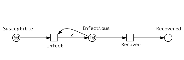
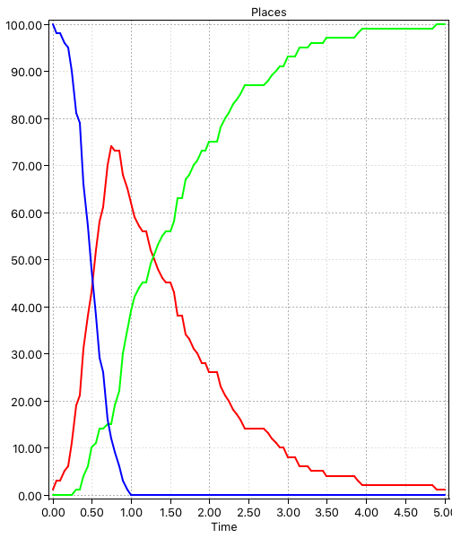
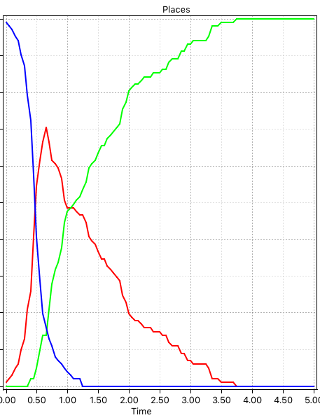
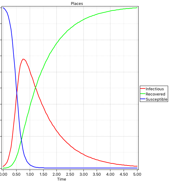
Figure 1: SIR model. (Top) A Petri Net describing the SIR model where Petri net places (circles) represent the Susceptible (S), Infectious (I) and Recovered (R) compartments. Petri net transitions (squares) represent the actions (events) of becoming infectious and recovering, and arcs connect places with transitions enabling events to occur and describing the effect of the occurrence. At the Infect transition, an infection will only occur when a susceptible and infectious person meet reducing the number in both compartments by 1. This results in two people being added to the Infectious place which is represented by an arc weight of 2 (shorthand notation for two arcs). Note that the default arc weight of 1 is not given. Also the number of infectious people can be reduced by 1 via the Recover transition, increasing Recovered by 1. Each transition preserves the number of persons (the number of incoming arcs equals the number of outgoing arcs), thus the net is conservative and the total population size is constant. (Bottom) From left to right: Two single stochastic runs and the deterministic run, with $S0=100$, $I0=1$, $k_{infect}=0.1$, $k_{recover}=1$. Note, in the second stochastic run, Infectious dies out much earlier than in the deterministic simulation.

We make some observations about the behaviour of the system. There is a trivial, i.e. disease free steady state for $I_{0}=0$ so that no infections or recovery occur, otherwise the steady state is reached when $I_{t}=0$. We note some interesting $\mathcal{SPN}$ behaviour of single runs – there is a probability that the infection dies out early, whatever the balance between the rates of infection and recovery, due to the underlying Markov chain. In contrast, the ODE behaviour can be thought of as the average over many stochastic runs, and thus ignores the variability inherent in a stochastic model. Besides exploring time series of model variables, we can also define derived measures as observers, such as the reproduction number $\mathcal{R}$ [HSW05, vdD17]; see Methods section for details.

All our models can be equally read as $\mathcal{SPN}$ or $\mathcal{CPN}$.

2.2 Extended epidemic models

The SIR model can be extended by extra compartments such as deaths (D), maternally-derived immunity (M), exposed/incubation period (E) etc., and extra variables such as total number of infectious, total deaths, yielding variations of the basic SIR model including SIS, SIRS, SIRD, MSIR, SEIR, SEIS, MSEIR, MSEIRS [Het00]. Their representation as a Petri net model is straightforward, and Petri net animation supports the modeller in getting the model structure right. Some illustrative models from this paper can be animated in a web browser at https://www-dssz.informatik.tu-cottbus.de/DSSZ/Research/ModellingEpidemics.

Here we consider two examples which are relevant to the current COVID19 epidemic (Figure 2):

• SIQR model which describes, as an additional route to recovery, the possibility of infectious people being subject to quarantine before recovery [ASGS20].

• SIAR model which differentiates infectious people into symptomatic and asymptomatic compartments [SIAQN17].

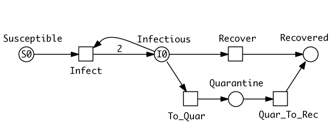
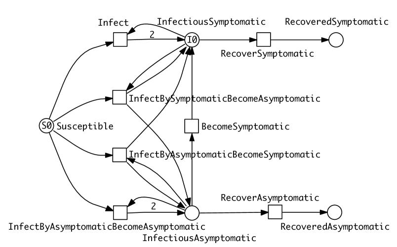
Figure 2: Two extended epidemic models. (Top) SIQR - an SIR model extended by quarantine. (Bottom) SIAR - an SIR model with symptomatic/asymptomatic compartments. There are four different cases of infection reflected by the four transitions connected with the Susceptible place. The two which involve only one infectious compartment – InfectiousSymptomatic or InfectiousAsymptomatic – follow the standard SIR pattern, reflected in the outgoing arc weights of 2. In the cases of the two dual outcome infections – Susceptible and InfectiousSymtomatic to InfectiousAsymptomatic or vice versa, there are two outgoing arcs to the two infectious places each of which has an arc weight of 1 (not shown by default). The total rate of infection in the whole population is the sum of the rates of the four infection transitions. The ODEs of these two models are given in the Supplementary Material.

2.3 Stratified epidemic models

In general, modelling the stratification of a population in terms of epidemics means that the overall population is partitioned into a number of strata and a suitable model is defined for each stratum and their appropriate interconnections. The compartments are equally divided into disjunctive sets, such that each partition is internally homogeneous and distinctively differs from all the other partitions, and there are corresponding partitions in all compartments.

In the following we assume that the same epidemic model is equally applied to each stratum. As an example we consider SIR-$\textrm{S}^{\textrm{age}}_{\textrm{2}}$, an SIR model with two age strata (Figure 3 (Top)). See Methods section for an explanation of our naming convention for models.

Clearly the stratification in this model is very minimal; the standard practice when collecting statistics of infections is to use more than two age groups - often in 10 deciles from 0 to 100 years old. A model should describe all the possible combinations of cross infections, in this case we obtain $10\cdot 10=100$ infect transitions. The modelling effort invites modelling errors; this will be further compounded if gender is added to age in the stratification. To cope with this modelling challenge, we use coloured Petri nets.

Coloured Petri nets

provide an elegant solution to the given combinatorial problem by pattern compression of the repeated parts of a Petri net, while maintaining the connections between those parts. Each repeated component is associated with a unique integer (‘colour’); see Methods section for details. This colouring principle can be equally applied to $\mathcal{SPN}$ or $\mathcal{CPN}$, yielding coloured $\mathcal{SPN}$ ($\mathcal{SPN^{C}}$) and coloured $\mathcal{CPN}$ ($\mathcal{CPN^{C}}$).

In summary, Figure 3 gives the same model in two different but equivalent representations, uncoloured (Top) and coloured (Bottom), which also means that both generate the same ODEs. Obtaining the coloured model from the uncoloured one is called folding, and the reverse operation is called unfolding. Folding is typically performed manually because the degree of folding is subjective, while unfolding can be done automatically as long as all colour sets are discrete and finite.

Increasing the number of strata while ensuring that all needed connectivities are present just requires extending the colour set Strata; nothing else in the structure of the coloured model needs to be touched, apart from adjusting the initial marking. In this way, our modelling approach supports scalability in an easy to use manner. In general the unfolded SIR model for $s$ strata comprises $3s$ places, $s^{2}+s$ transitions and $4s^{2}+2s$ arcs, and the ODEs generated consist of $3s$ equations.

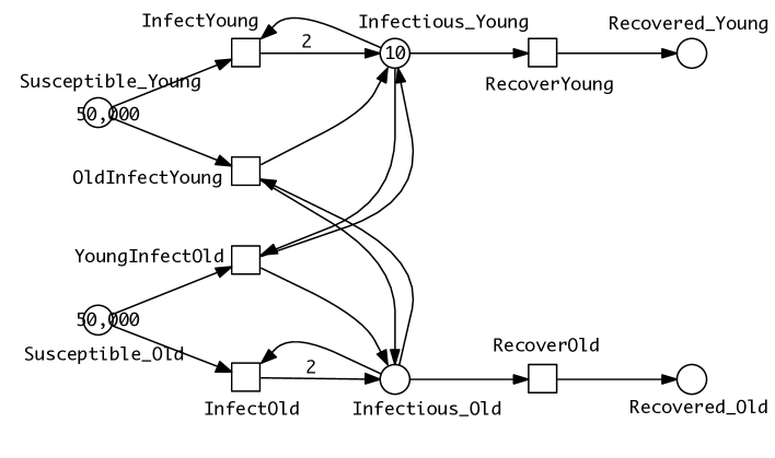
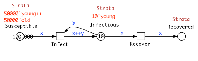
Figure 3: SIR-$\textrm{S}^{\textrm{age}}_{\textrm{2;20}}$ models. Two variations of the SIR model describing stratification of a population into two age groups (young and old) or 20 age groups, and the cross infections between the groups. Transmission of infection does not change the age group of the infectious person. At the start there are no old infectious people, and only very few young infectious people. (Top) $\mathcal{CPN}$ for two age strata, each of which is associated with a separate, but structurally identical SIR model, and linked by cross infections. (Middle) The same model represented as a coloured $\mathcal{CPN}$. The markings of coloured places always show the sum of the markings of the corresponding uncoloured places. The colour definitions are given in the Methods section, and the ODEs in the Supplementary Material. (Bottom) Unfolded $\mathcal{CPN}$ of a 20-strata SIR model, with coloured graphics.

2.4 Pandemic models

The distinguishing characteristic of a pandemic model is the concept of multiple intercommunicating epidemic models in a spatial (geographic) context. In the following we prefix standard epidemic model names by ‘P’ for pandemic, thus obtaining PSIR, PSIQR, etc.

Two countries, linked by travel.

Figure 4 (Top) shows a PSIR model comprising epidemic SIR models in each of two countries, with population movement permitted between the countries for all compartments. As for the age strata model, we can fold it into a coloured version (Figure 4 (Bottom)). The process of colouring is very similar to that described for SIR-$\textrm{S}^{\textrm{age}}_{\textrm{2}}$ (see Methods section).

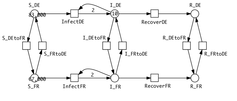
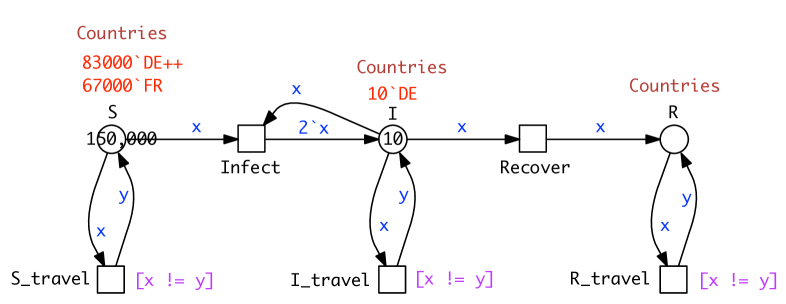
Figure 4: P₂SIR model. (Top) $\mathcal{CPN}$ for two countries, each of which is associated with a separate, but structurally identical SIR model, and linked by travel. (Bottom) The same model represented as a coloured $\mathcal{CPN}$. Eeach travel transition is associated with a guard [x != y] (x and y are unequal) to ensure that travellers do not immediately return to their country of origin. The uncoloured and coloured model are equivalent, thus generate the same ODEs, which are given in the Supplementary Material.

N countries, linked by travel.

Generalising this idea to more than two countries, the travel connectivities between countries need to be defined. For example when considering surface travel, not all countries are directly connected to each other. We assume that the connectivity is described by a graph (Figure 5 (Top left)); this could be directly encoded as a standard Petri net (Figure 5 (Top middle)), which we fold for convenience into a coloured Petri net (Figure 5 (Top right)), see Methods section for details. Equally the graph could include air and/or sea connections; even then, connectivity could still be less than fully connected.

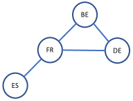
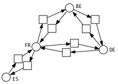
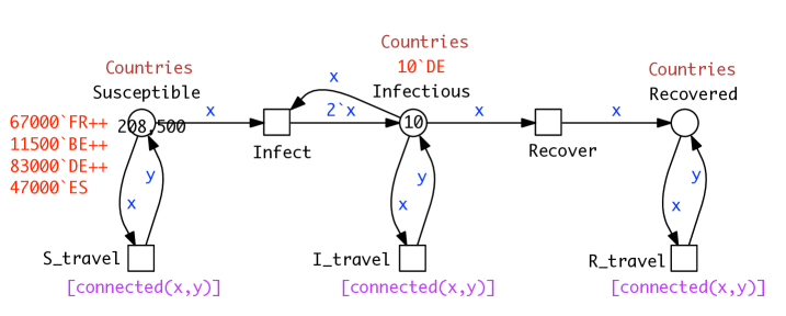
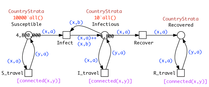
Figure 5: P_nSIR models. (Top left) Connectivity graph for four countries. (Top middle) Petri net representation of the connectivity graph. (Top right) Coloured Petri net representation of the connectivity graph; see Methods section for details. (Middle) Coloured Petri net representation of the pandemic P₄SIR; structural identical with P₂SIR in Figure 4 (Bottom); both $\mathcal{CPN^{C}}$ differ by their colour definitions encoding different connectivity graphs. The unfolded Petri net of P₄SIR is give in Figure C.2. (Bottom) P${}_{\textrm{48}}$SIR-$\textrm{S}^{\textrm{age}}_{\textrm{10}}$ coloured Petri net for 48 countries in Europe, each with 10 age strata, see Figure 6 for its unfolded version.

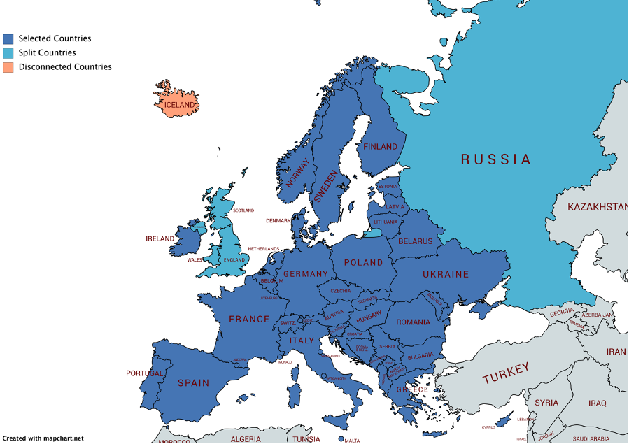
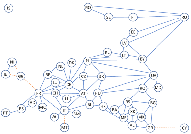
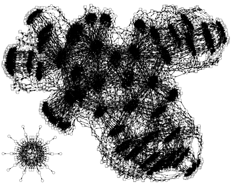
Figure 6: P${}_{\textrm{48}}$SIR-$\textrm{S}^{\textrm{age}}_{\textrm{10}}$ model. (Top left) Map of 48 European countries created with https://mapchart.net. (Top right) Undirected graph representation of the map where edges represent two-way surface connections. Blue edges stand for road connections, orange dashed edges for sea connections. (Bottom) Unfolded version of the coloured net in Figure 5 (Bottom); layout automatically generated. Iceland appears as an isolated subnet because it is not connected by surface to the rest of Europe, and is thus similar to the SIR net with 20 strata in Figure 3 (Bottom). Model size: 1,440 places; 10,380 transitions.

The coloured Petri net representation of the PSIR over four countries (Figure 5 (Middle)) is derived by adjusting the colour definitions in the SIR for two countries (Figure 4 (Bottom)) according to the connectivity graph, and getting the initial marking right.

The generalisation to connectivity graphs representing different geographical relationships is straightforward, merely requiring adjusting the two related colour definitions (Countries, Connections) and the initial marking. This example illustrates how our modelling approach supports reusability in an easy to use manner. In general the unfolded PSIR model for $n$ countries with overall $m$ mutual connections comprises $3n$ places, $2n+6m$ transitions and $6n+12m$ arcs, and the ODEs generated consist of $3n$ equations.

We provide a number of PSIR pandemic models in the Supplementary Material, including Europe (P₁₀SIR – 10 countries, 15 mutual connections, P₄₈SIR – 48 countries, 85 mutual connections), China (P${}_{\textrm{China}}$SIR – 34 provinces, 71 mutual connections) and the USA (P${}_{\textrm{USA}}$SIR – 50 states, 105 connections), and the guidelines how to obtain the corresponding ODEs using our tool platform.

2.5 Combined models

These three extensions – SIR variations, stratification and space – are orthogonal, and thus any combination is possible. For illustration we provide two examples:

• P₁₀SIQR combining space (Europe with 10 countries) with an extended epidemic model (see Figure C.3) which yields $4n=40$ ODEs, and

• P₄₈SIR-S${}^{\textrm{age}}_{10}$ combining space (Europe with 48 countries) and stratification (10 age strata per country; coloured version in Figure 5 (Bottom), unfolded version in Figure 6) which yields 1440 ODEs.

  In general the unfolding of a P_nSIR-S_s model with $s$ strata and $n$ countries with $m$ mutual connections comprises $3sn$ places, $n(s^{2}+s)+6ms$ transitions and $2n(2s^{2}+s)+12ms$ arcs.

2.6 Parameter fitting

Apart from defining the structure of a model, it is also important to find suitable rate constants. This can be naively achieved by scanning over parameter values, or in a more sophisticated manner heuristically by target driven parameter optimisation.

Even without fitted values derived from real world data, a great deal of useful analysis can be achieved using comparative rate constant values. Examples include scanning by

• varying the ratio between infection rate and recovery rate while maintaining the recovery rate constant resulting in changes in the $\mathcal{R}$_t value (SIR), and comparison between geographic regions (PSIR),

• varying the ratio between direct and quarantine recovery (SIQR), and varying quarantine regimes (Figures C.4, C.5, both referring to the model P₁₀SIQR in Figure C.3 (Top)).

• varying the initial state of the infectious compartments in the different countries of a pandemic model (PSIR),

• varying the strength of the connectivities between countries - road, train, sea and air - in a pandemic model (PSIR).

Refining a model automatically involves increasing the number of required kinetic rate constants. Specifically in the SIR-$\textrm{S}^{\textrm{age}}_{\textrm{2}}$ model, the kinetic constants can be different for both intra-stratum and inter-strata transitions. This can be achieved in the coloured version using colour-dependent rates, see Methods section.

More generally, we can establish equivalence classes for rate constants, for example in a PSIR travel model, there can be different rate constants between classes of movements such as road versus air and/or frequent versus rare, while the rate constants within classes are the same.

When real world data are available, then we can attempt to fit models to them. We did this for the pandemic model for ten European countries (P₁₀SIR, see Figure C.6), based on source data for daily new infections obtained from WorldOmeters (https://www.worldometers.info/coronavirus/) during the period 19th January to 16th August 2020. The rate constants fitted were for infection, and the inter-country movement for all three compartments. The values for the Susceptible, Infectious and Recovered compartments for movement in one direction between a pair of countries were kept the same, thus reflecting the assumption that the rate constant for travel does not depend on the compartment, but only on the journey. Initial markings for Infectious were set at 1% of the total population for each country according to Wikipedia, divided by 1000. Daily new cases were standardised and smoothed using a 7-day rolling average (Figure C.7) and the magnitude and timing of the peaks were detected computationally (Table C.1).

The goals of the fitting were (Objective 1) to reproduce the order of the time taken from the first 5 deaths to a peak for daily new cases, (Objective 2) to reproduce the order of the height of the peaks for daily new cases, and (Objective 3) combining Objective 1 and Objective 2. Fitting was performed in all three cases using target driven optimisation employing Random Restart Hill Climbing (see Methods section for details, and Tables C.2 – C.5).

2.7 Analysis

For an initial validation of (unfitted) pandemic model behaviour we performed correlation analyses between real world variables and model variables for P₁₀SIR and P₄₈SIR; for details see Table C.6 and Figures C.10, C.12. These results support our assumption that even the unfitted pandemic models behave well, and that the geography incorporated into the model appropriately influences behaviour. Thus, an analysis of the unfitted pandemic PSIR model can give useful insights even in the absence of detailed real data; specifically given the geographical connections between regions and their populations, we can predict to some extend the expected peak height of infections and thus inform planners how to cope with the impact on health services etc.; some examples are given below.

An initial analysis can be performed by inspection of the visualised time series plots. Properties of interest include the values of Susceptible and Recovered over time (e.g. for herd immunity), and the existence, order and height of peaks for Infectious, see e.g. Figure C.8. This can be extended to derived measures such as the $\mathcal{R}$ value, computed over time and plotted for the different geographic regions.

Going beyond visual inspection, the order and height of peaks can be ascertained computationally from the traces. More generally, many behavioural properties of interest can be expressed using linear temporal logic and analysed in practice via simulative model checking [DG08, GHGC19], which is specifically useful for exploring larger models by the use of property libraries, see Methods section and Figure C.9.

In addition, the general relationships between the behaviour of related compartments or derived measures in different geographical regions can be determined via cluster analysis. The results for hierarchical clustering can be represented for example via dendrograms, see Figures C.13, C.14.

Furthermore, the results of such comparative analyses above could be related to the genomic data of the causative infectious agent, for example a virus which exhibits high mutation rates. Thus the variants or strains of the virus which evolve over the time of an epidemic can be related to the behaviour of pandemic models.

Finally, pandemic models can be used to predict the effects of various control measures. These include travel restrictions in terms of inter-country connections, and quarantine restrictions on international travellers. In addition, the effects of the imposition and lifting of lockdowns in different regions and at different times can be investigated, but requires the dynamic variation of rate constants during simulation. In order to facilitate this, we have recently extended the Spike simulator to include event-driven triggers, which enables the modelling of these control measures, see for example Figure C.16.

Given a pandemic PSIR model with fitted parameters, as developed in the previous section, we can perform a detailed comparative analysis over the geographic regions, going beyond the analysis based on comparative values;

3 Methods

Related work.

In order to put our work in context, we give a brief overview of related work. A general review paper on epidemic modelling including metapopulation models can be found in [Bra17]. Early basic pandemic approaches include mathematical models based on ODEs for the global spread diseases, where travel connectivity is described by adjacency matrices [RLJ85, LJ88], and by graphs [SP93, SD95].

The GLEaMviz computational tool [VdBGG⁺11] has been developed to model multiscale mobility networks and the spatial spreading of infectious diseases building on a series of papers including [CV08, BCG⁺09, BGH⁺10] and has been used to model the 2009 H1N1 pandemic [BPR⁺11]. Some more recent work by other groups includes [CYX14] considering dynamics of a two-city SIR epidemic model and [ABCC⁺20, GS20] for the current COVID19 pandemic.

The Spatiotemporal Epidemiologic Modeler (STEM) is an Eclipse based monolithic framework to support the development and simulation of geographic disease models [EDK10]. It builds on a component-based architecture (plugins); models can be simulatated deterministically or stochastically. Models are encoded in Java, and it is not obvious how to export a model if one wants to apply any analysis technique not supported by the framework.

Age-based stratification has been addressed in, for example, [DVHC13, BM20], and the effects of intervention strategies for COVID19 in [BM20, PLR⁺20, GBB⁺20].

Other approaches besides ODE modelling include stochastic models [NA19, OWZ20], agent based models [MAS⁺20] and coloured Petri nets [CPG⁺20].

In the following we describe the methods underlying our technology.

3.1 Modelling

SIR modelling assumptions.

The population in the SIR model population is divided into three compartments – Susceptible (S), Infectious (I) and Recovered (R). These three compartments are considered to be homogeneous, thus there is an equal probability of any event occurring to any member of each compartment. In general, this assumption of homogeneity applies to any compartment in our models.

A susceptible person is infected by an infectious person so that they are both infectious; thus getting infected and becoming infectious coincide. A susceptible person can become recovered. Recovered people are resistant and cannot become susceptible or infectious. This simple model does not consider births, or natural deaths so that the total population size is constant, as can be seen from the structure of the SIR model in Figure 1, which shows a conservative Petri net covered by a single minimal P-invariant (compare paragraph below on Petri net analysis techniques). It is also generally assumed that $S_{0}\gg I_{0}$, and (for obvious reasons) $I_{0}>0$ and $R_{0}=0$.

Petri nets

are a family of formal languages which come with a graphical representation as bipartite directed multi-graphs, enjoying an operational (execution) semantics. They can be either untimed and qualitative, or timed and quantitive; for details see [HGD08]. All these net classes share the following graph properties.

• Bipartite: There are two types of nodes, called places and transitions, which form disjunctive node sets. Places, graphically represented as circles, typically model passive objects (here compartments and derived measures, possibly in different locations), while transitions, graphically represented as squares, model active events (such as infect, recover, travel), changing the state of the passive nodes.

• Directed: Directed arcs, represented as arrows, connect places with transitions and vice versa, thereby specifying the relationship between the passive and active nodes. The bipartite property precludes arcs between nodes of the same type.

• Multigraph: Two given nodes may be connected by multiple arcs, typically abbreviated to one weighted arc. The weight is shown as a natural number next to the arc. The default value is 1, and usually not explicitly given.

The execution semantics builds on movable objects, represented as tokens residing on places. The number zero is the default value, and usually not explicitly given. The current state (marking $m$) of a model is defined by the token situation on all places, usually given by a place vector, which is a vector with as many entries as we have places, and the entries are indexed by the places. The initial state is denoted by $m_{0}$.

The specific details of the execution semantics slightly differ for qualitative and quantitative Petri nets, and if the Petri net class belongs to the discrete or continuous modelling paradigm.

We start off with standard Petri nets, which are inherently untimed and discrete. Their (non-negative integer) token numbers are given by black dots or natural numbers. The current state is given by the number of tokens on all places, forming a place vector of natural numbers. The (integer) arc weights specify how many of these tokens on a certain place are consumed or produced by a transition, causing the movement of tokens through the net, which happens according to the following rules (see [BHM15]):

• Enabledness: A transition is enabled, if its pre-places host sufficient amounts of tokens according to the weights of the transition’s ingoing arcs. An enabled transition may fire (occur), but is not forced to do so.

• Firing: Upon firing, a transition consumes tokens from its pre-places according to the arc weight of the ingoing arcs, and produces new tokens on its post-places according to the arc weights of the outgoing arcs. The firing happens atomically (i.e., there are no states in between) and does note consume any time. Firing generally changes the current distribution of tokens; thus the system reaches a new state.

• Behaviour: We obtain the dynamic behaviour of a Petri net by repeating these steps of looking for enabled transitions and randomly choosing one single transition among the enabled ones to let it fire.

Rate functions.

These standard untimed Petri nets, which are entirely qualitative, can be extended by enriching transitions with firing rate functions. We obtain timed and thus quantitive Petri nets, out of which we use in this paper stochastic Petri nets ($\mathcal{SPN}$) generating continuous time Markov chains, and continuous Petri nets ($\mathcal{CPN}$) generating Ordinary Differential Equations (ODEs). Both net classes merely differ by the interpretation of the rate functions; thus $\mathcal{SPN}$ and $\mathcal{CPN}$, sharing the same net structure, can be easily converted into each other.

Rate functions are, technically speaking, arbitrary mathematical functions, typically depend on the given state, and are often governed by popular kinetics, such as mass action kinetics [WW45].

Stochastic rate functions specify how often a transition occurs per time unit, technically achieved by stochastic waiting times before an enabled transition actually fires. $\mathcal{SPN}$ with exponentially distributed waiting times for all transitions fulfil the Markov property; thus their semantics are described by continuous time Markov chains (CTMC), and the current state of an SPN is still defined by a place vector of natural numbers. The CTMC for a given $\mathcal{SPN}$ is basically isomorphic to the state transition system of its corresponding untimed Petri net. Thus, all Petri net analysis techniques see paragraph on Petri net analysis below) can still be applied, and all behavioural properties that hold for the untimed Petri net are still valid for the corresponding $\mathcal{SPN}$.

In contrast, deterministic rate functions define the strength of a continuous flow, turning the traditionally discrete modelling paradigm of Petri nets into a continuous one: the discrete number of tokens on each place is replaced by a (non-negative) real number, called token value. Thus, the current state of a $\mathcal{CPN}$ is defined by a place vector of real numbers. A $\mathcal{CPN}$ transition is enabled if the token value of all its pre-places is larger than zero. This coincides for mass action kinetics with transition rates larger than zero. Due to the influence of time, a continuous transition is forced to fire as soon as possible. Altogether, the semantics of a $\mathcal{CPN}$ is defined by ODEs.

How to transform a $\mathcal{CPN}$ into ODEs.

Each place subject to changes gets its own equation, describing the continuous change over time of its token value by the continuous increase of its pre-transitions’ flow and the continuous decrease by its post-transitions’ flow. Thus, in the generated ODEs, places are interpreted as (nonnegative) real variables. A transition that is pre- and post-transition for a given place yields two terms, which can be reduced by algebraically transforming the right-hand side of the equation. Thus, each equation corresponds basically to a line in the incidence matrix [HGD08].

To formalise the transformation of $\mathcal{CPN}$ into ODEs, we need to introduce a few technical notations. Let ${{}^{\bullet}}p$ denote the set of pre-transitions of the place $p$, and $p\,{{}^{\bullet}}$ the set of post-transitions, $v\left(t\right)$ gives the rate function for transition $t$, $f\left(t,p\right)$ the weight of the arc going from $t$ to $p$, and $f\left(p,t\right)$ the weight of the arc going from $p$ to $t$. Then the ODE generated for the place $p$ is given by Equation 2.

$$\frac{d\left(p\right)}{dt}=\sum_{t\in{{}^{\bullet}}p}f\left(t,p\right)v\left(t\right)-\sum_{t\in p\,{{}^{\bullet}}}f\left(p,t\right)v\left(t\right)$$ (2)

In words: the pre-transitions $t\in{{}^{\bullet}}p$ increase the token value of $p$, thus their weighted rate functions occur as plus terms, while the post-transitions $t\in p\,{{}^{\bullet}}$ decrease the token value of $p$, thus their weighted rate functions occur as minus terms of the ODE’s right hand side.

The models presented in this paper always generate as many ODEs of this style as we have places. This is automatically triggered when simulating a $\mathcal{CPN}$, which can be done in our platform either with Snoopy or Spike. In summary, $\mathcal{CPN}$ can be seen as a structured approach to write ODEs [BGHO08]; they uniquely define ODEs, but generally not vice versa, compare [SH10, HG11].

Coloured Petri nets

combine Petri nets with the powerful concept of data types as known from programming languages [GL81, JK09]. Tokens are distinguished via colours; there are no limits for their interpretation. For example, colour allows for the discrimination of compartments by, e.g., age strata or gender, or to distinguish compartments in different geographical locations. In short, colours permit us to describe similar network structures in a compressed, but still readable way. A group of similar model components (subnets) is represented by one component coloured with an appropriate colour set, and the individual components become distinguishable by a specific colour in this colour set. See [LHG19] for a review of the widespread use of coloured Petri nets for multilevel, multiscale, and multidimensional modelling of biological systems.

Coloured Petri nets consist, as uncoloured Petri nets, of places, transitions, and arcs. Additionally, a coloured Petri net is characterised by a set of discrete data types, called colour sets, and related net inscriptions.

• Places get assigned a colour set and may contain a multiset of distinguishable tokens coloured with colours of this colour set. Our PetriNuts platform supports a rich choice of data types for colour set definitions, including simple types (dot, integer, string, boolean, enumeration) and product types.

• Transitions get assigned a guard, which is a Boolean expression over variables, constants and colour functions. The guard must be evaluated to true for the enabling of the transition. The trivial guard true is usually not explicitly given.

• Arcs get assigned an expression; the result type of this expression is a multiset over the colour set of the connected place.

• Rate functions may incorporate predicates, which are again Boolean expressions. They permit us to assign different rate functions for different colours (colour-dependent rates). Otherwise, the trivial predicate true is used; for examples see Supplementary Material.

Elaborating the behaviour of a coloured Petri net involves the following notions (see [BHM15]).

• Transition instance: The variables associated with a transition consist of the variables in the guard of the transition and in the expressions of adjacent arcs. For the evaluations of guards and expressions, values of the associated colour sets have to be assigned to all transition variables, which is called binding. A specific binding of the transition variables corresponds to a transition instance. Transition instances may have individual rate functions.

• Enabling: Enabling and firing of a transition instance are based on the evaluation of its guard and arc expressions. If the guard is evaluated to true and the pre-places have sufficient and appropriately coloured tokens, the transition instance is enabled and may fire. In the case of quantitative nets, the rate function belonging to the transition instance is determined by evaluating the predicates in the rate function definition.

• Firing: When a transition instance fires, it consumes coloured tokens from its pre-places and produces coloured tokens on its post-places, both according to the arc expressions. which generally results into a new state.

Colouring example.

Let us illustrate the use of colour by means of the stratified age SIR example (SIR-$\textrm{S}^{\textrm{age}}_{\textrm{2}}$), see Figure 3. The common pattern is a single basic SIR model. In order to design the coloured model, shown in Figure 3 (Bottom), we introduce an enumerated colour set Strata = {young, old} (where each element is internally mapped onto an integer) and two variables of this colour set x and y, each of which can hold either young or old. Arcs in this model are now labelled with expressions over these variables. The bindings to the variables are considered only in the local environment (incoming and outgoing arcs) of each transition. The incoming and outgoing arcs of the coloured transition Recover are both labelled with the same variable x because that transition only operates within one stratum. However the coloured transition Infect has connections both within one stratum and between strata; this is accomplished by using the two variables x and y on the two incoming arcs from Susceptible and Infectious, each of which independently hold as bindings either young or old, giving in total four combinations, two of which standing for the inter-strata cross infections and the other two for the intra-stratum infections. The x represents the person who becomes infectious, and y the infecting person. Thus the outgoing arc from the transition to the place Infectious is labelled with the multiset {x,y} written as x++y. If x and y hold the same colour, x++y corresponds to an arc weight of 2 in the standard Petri net model.

Folding/Unfolding.

Any (standard) Petri net can be folded into a coloured Petri net comprising just a single (coloured) place and a single (coloured) transition. Then, the entire structure is hidden in the colour definitions, which can always be revealed by automatic unfolding. Generally, the decision regarding how much structure to fold into colours is a matter of taste. We follow the rule that a model should be still completely comprehensible by reading the structure and its colour annotations. In general, folding of epidemic models should preserve the pattern of the SIR (or related) model. For illustration, we provide a coloured version of the SIAR symptomatic/asymptomatic model in the Supplementary Material.

In principle, coloured Petri nets could be simulated directly on the coloured level, thus avoiding blowing up the model structure which often comes with unfolding. However, the corresponding algorithms are much more complicated, often involve an implicit partial unfolding, and only a few of them are actually available in practice [BFF⁺15].

In contrast, unfolding to the corresponding uncoloured Petri net can be efficiently achieved [SRL⁺20] and permits to re-use the rich choice of analysis and simulation techniques, which have been developed over the years for uncoloured Petri nets, including $\mathcal{SPN}$ and $\mathcal{CPN}$, many of them are now supported by highly efficient libraries and reliable software tools.

This is why we exclusively adopt the second approach. All our coloured models are automatically unfolded when it comes to analysing and/or simulating them.

Encoding space and locality.

The use of colour enables us to encode matrices, where colours (natural numbers) represent indices; multidimensional matrices can be represented by appropriate colour tuples. Previously we have used this approach to encode one, two and three dimensional Cartesian space where coordinates were represented as tuples over the entire matrix [GHLS13], for example modelling diffusion and cell movement in biological systems: planar cell polarity in the Drosophila wing [GGH⁺13], phase variation in bacterial colonies [PGH⁺15], bacterial quorum sensing [GHGC19] and intra-cellular calcium dynamics [IHAH20].

In this research we use tuples to index sub-matrices, permitting us to represent graphs as adjacency matrices and hence to encode geographical spatial relationships. This overcomes the limitations of the previous Cartesian coordinate approach for representing pandemics, because whole matrices represent travel diffusion-wise in a regular grid, rather than specific travel connections.

For illustration we consider the encoding of the connectivity graph for four European countries, see Figure 5 (Top). In order to achieve this we define a colour set of enumeration type comprising all countries and next a matrix as a product over this colour set.

colorsets:
  enum Countries = {BE,DE,ES,FR};
  Matrix = PROD(Countries,Countries);

A subset of the matrix is defined by a Boolean expression (given in square brackets) comprising all required connections.

colorsets:
  Connections = Matrix[  // subset defined by Boolean expression
    (x=ES & (y=FR)) |
    (x=FR & (y=ES | y=BE | y=DE)) |
    (x=BE & (y=DE | y=FR)) |
    (x=DE & (y=FR | y=BE ))];

Finally we define a colour function connected to be used as guard for the Travel transitions, which constrains travel according to the connectivity graph.

colorfunctions:
bool connected(Countries p, Countries q) { (p,q) elemOf Connections };

This acts in the same way as the more simple constraint [x != y] used in Figure 4. Now, colour-dependent rates may model different disease control policies in different subpopulations or in different locations.

Besides this, we need two variables of the colour set Countries to be used in the arc inscriptions and thus occurring as parameters in the transition guard.

variables:
  Countries : x;
  Countries : y;

Framework.

These colouring principles can be equally applied to qualitative and quantitative Petri nets, yielding, among others, coloured $\mathcal{SPN}$ ($\mathcal{SPN^{C}}$) and coloured $\mathcal{CPN}$ ($\mathcal{CPN^{C}}$): Our PetriNuts platform supports the handling of all of them, which includes the reading of a quantitative Petri net as either $\mathcal{SPN}$ or $\mathcal{CPN}$ (supported by Snoopy and Spike) and the automatic unfolding of $\mathcal{SPN^{C}}$ and $\mathcal{CPN^{C}}$ to their uncoloured counterparts (supported by Snoopy, Marcie and Spike).

See Figure A.1 for an overview of the modelling paradigms integrated in the unifying framework of the PetriNuts platform and the relations among the supported net classes [HHL⁺12].

Petri net analysis techniques.

Petri net theory comes with a wealth of analysis techniques [Mur89], some of them are particularly useful in the given context due to the specificity of the net structures of our $\mathcal{SPN}$/$\mathcal{CPN}$ models, which we obtain by design.

• Conservative: A Petri net is called conservative, if the number of tokens is preserved by any transition firing. This is the case if it holds for all transitions that the sum of the weights of incoming arcs equals the sum of the weights of outgoing arcs. In our models, most of the transitions have exactly one incoming and one outgoing arc, with the exception of Infect transitions which have two incoming and two outgoing arcs (the latter combined to one arc with a weight of 2).

• P-invariant: A P-invariant (as it occurs in the models considered here) corresponds to a set of places, holding in total the same amount of tokens in any reachable state. Generally, P-invariants induce token-preserving subnets. A P-invariant is minimal, if (roughly speaking) it does not contain a smaller P-invariant; see [Hei09] for details. The models discussed in this paper have the remarkable property that the are covered by non-overlapping minimal P-invariants, and each minimal P-invariant comprises the places (compartments) of one stratum.

  Extending a model by cumulative counters, such as the total number of infectious over time, destroys the conservative net structure and induces additional overlapping P-invariants; thus the model is still covered with P-invariants (CPI); see Figure C.3 for an example.

  More generally speaking, any epidemic/pandemic model without birth (transition without pre-place) and/or death (transition without post-place) is covered with P-invariants.

We use both criteria for model validation to avoid modelling mistakes. They are independent of the initial marking and can be decided by exploring the net structure only. This is done in our PetriNuts platform by the tool Charlie. Both criteria prove independently the boundedness of a model (the number of tokens on each place is limited by a constant), which ensures in turn a finite state space.

The finite state space could possibly open the door to analyse $\mathcal{SPN}$ models by numerical methods to determine popular Markov properties [SH09], such as the probability to reach a (transient) state where, e.g., half of the population is effected. A closer look on the typical size of the generated CTMC however soon questions this endeavour, as numerical methods rely on a real-numbered square matrix in the size of the state space [HRSS10]. So we basically have to confine ourselves to simulation and analysis techniques working over simulation traces, such as simulative model checking; see Methods subsection on Analytical methods.

It is obvious from exploring the model behaviours that they reach a dead state (there is no enabled transition), as soon as the infectious compartment becomes empty, because there is no way to add something to the infectious compartment as soon as it got empty. In Petri net terms this corresponds to a bad siphon (a siphon not containing a trap); all these are further popular notions of Petri net theory, requiring structural analysis only, while permitting conclusions on behavioural properties; see [HGD08] for details.

Often, epidemic/pandemic models are by design irreversible, reflecting the (optimistic) assumption that a once gained immunity is never lost, and a model will reach a dead state at the very latest when the entire population is recovered. Loosening this assumption by adding a transition from either Infectious or Recovered to Susceptible and refilling Infectious in each epidemic model component will introduce cycles to a model which now becomes a chance to be reversible and live (which in turn precludes dead states), if it is covered with T-invariants (see [Hei09] for details). This obviously requires that the geographical connectivity graph is strongly connected.

Petri net simulation.

Besides structural analysis for model validation, we apply simulation techniques generating traces of model behaviour. Simulation traces are time series reporting the current variable values at the $n+1$ time points $t_{i}$ of a specified output grid $i=0,\dots n$, typically splitting the simulation time into $n$ equally sized time intervals. We consider here two basic types of traces:

• traces of place markings, i.e., time series of the current marking (state) of the compartments at the specified time points of the simulation run:

  $s(t_{i}):P\rightarrow{\mathbb{N}}$, with $s(t_{0})=m_{0}$,

  i.e., $s(t_{i})$ are (non-negative) integer place vectors over all place markings, indexed by the set of places $P$.

• traces of transition rates, i.e., time series of the number of occurrences which each individual event had in total in the latest time interval,

  $v(t_{i}):T\rightarrow{\mathbb{N}}$, with $v(t_{0})=0$,

  i.e., $v(t_{i})$ are (non-negative) integer transition vectors over all transition rates, indexed by the set of transitions $T$.

Reading a transition rate vector as Parikh vector immediately leads us to the state equation specifying the relation between both traces:

$s(t_{i})=s(t_{i-1})+{\mathbb{C}}\cdot v(t_{i}),i=1\dots n$,

where ${\mathbb{C}}$ is the incidence matrix of a Petri net (see [HGD08]). Thus, the place trace can be derived from the transition trace, but generally not vice versa. In the stochastic setting, the transition trace cannot be uniquely deduced from the place trace due to alternative and parallel transitions, which specifically holds for individual traces. Therefore, we directly record the transition traces during simulation.

Often we consider averaged traces, and the deterministic simulation of $\mathcal{CPN}$/$\mathcal{CPN^{C}}$ is bound to do so, such that the individual values at each time point are non-negative real numbers (${\mathbb{R^{+}}}$) instead of natural numbers (${\mathbb{N}}$):

$s(t_{i}):P\rightarrow{\mathbb{R^{+}}}$, with $s(t_{0})=m_{0}$ (traces of place markings),

$v(t_{i}):T\rightarrow{\mathbb{R^{+}}}$, with $v(t_{0})=0\;\;\;$ (traces of transition rates).

Simulation traces may include coloured places/transitions, where a coloured node always gives the sum of the values of the corresponding unfolded nodes. For example, in the SIR-S₂ model given in Figure 3, the coloured place Susceptible always shows the sum of its two unfolded nodes Susceptible_Young and Susceptible_Old; likewise for transitions and their rates.

Derived measures.

A measure often used in the daily news is the daily or weekly number of new infections, given at time point $t$ by

$$\Delta^{I1}_{t}=S_{t}-S_{t-1}\;\;or\;\;\Delta^{I7}_{t}=S_{t}-S_{t-7}\;.$$

These can also be defined by:

$$\Delta^{I1}_{t}=(I_{t}-I_{t-1})+(R_{t}-R_{t-1})\;\;or\;\;\Delta^{I7}_{t}=(I_{t}-I_{t-7})+(R_{t}-R_{t-7})\;.$$

These numbers are typically normalised to a specific population size, e.g., 100,000, thus permitting the comparison of the local incidence numbers among regions.

A more scientific measure for characterising the progress of an epidemic is the reproduction number $\mathcal{R}$ [HSW05, vdD17] which is the average number of secondary cases produced by one infectious individual introduced into a population of susceptible individuals. It allows modellers to work out the extent of the spread, but not the rate at which the infection grows [Ada20]. This measure has several interpretations. $\mathcal{R}$₀ assumes that everybody in a population is susceptible to infection; this is only true when a new virus is introduced into a population which has never experienced it before and is a measure of the potential virulence of the disease. $\mathcal{R}$_t (sometimes called $\mathcal{R}$_e, or ‘effective $\mathcal{R}$’), is calculated over time as an epidemic progresses, and is a measure of the potential virulence of the disease. The value of $\mathcal{R}$_t varies during the course of an epidemic, as people gain immunity after an infection or a vaccination, or have adjusted their social interactions. Thus generally it holds that $\mathcal{R}$_t $\leq$ $\mathcal{R}$₀.

In our SIR model, we calculate $\mathcal{R}$_t for a time window of 1 by Equation 3; the generalisation to wider time windows is straightforward.

$$\mathcal{R}_{t}=\Delta^{I1}_{t}/\Delta^{I1}_{t-1}$$ (3)

$$\mathcal{R}_{t}=(S_{t}-S_{t-1})/(S_{t-1}-S_{t-2})$$

$$\mathcal{R}_{t}=((I_{t}-I_{t-1})+(R_{t}-R_{t-1}))/((I_{t-1}-I_{t-2})+(R_{t-1}-R_{t-2}))$$

Naming convention.

The naming convention of our models basically follows this Extended BNF. For a summary of the models provided see Table 1.

ModelName ::= [PandemicComponent] EpidemicComponent [‘-’ StratifiedComponent]
PandemicComponent ::= ‘P’ [Parameter] [PandemicRest]
PandemicRest ::= ‘Q’
Parameter ::= Number | Country
Country ::= ‘USA’ | ‘China’
EpidemicComponent ::= ‘S’ ‘I’ [EpidemicOption] ‘R’
EpidemicOption ::= ‘A’ | ‘V’ | ‘Q’
StratifiedComponent ::= ‘S’ {StratificationParameter}⁺
StratificationParameter ::= Type Number
Types ::= age | gender | $\epsilon$

Table 1: Summary table of models. I Basic and extended epidemic models. II Stratified models. III Pandemic models. IV Combined models; CANDL files provided as separate files in Supplementary Material.

Type	Id	Long name	Reference
I	SIR	standard SIR model	Figure 1
	SIVR	SIR with disease variant	Figure C.1
	SIQR	SIR with local quarantine	Figure 2 (Top)
	SIAR	SIR with asymptomatic infectious	Figure 2 (Bottom)
II	SIR-S	Stratified SIR
	SIR-$\textrm{S}^{\textrm{age}}_{\textrm{2}}$	Stratified SIR, 2 age strata	Figure 3 (Top/Middle)
	SIR-S10	Stratified SIR, 10 age strata
	SIR-$\textrm{S}^{\textrm{age}}_{\textrm{20}}$	Stratified SIR, 20 age strata	Figure 3 (Bottom)
	SIR-$\textrm{S}^{\textrm{age,gender}}_{\textrm{10x2}}$	Stratified SIR, 10 age and 2 gender strata
III	PSIR	Pandemic SIR
	PnSIR	Pandemic SIR, $n$ locations	Figure 4:(n=2), Figure 5:(n=4)
	P10SIR	Pandemic SIR with CummulativeInfectious, Western Europe (10 countries, 15 mutual connections)	Figure C.6, P10SIR.candl
	P48SIR	Pandemic SIR for Europe (48 countries, 85 mutual connections)	P48SIR.candl
	P${}_{\textrm{China}}$SIR	Pandemic SIR for China (34 provinces, 71 mutual connections)	PchinaSIR.candl
	P${}_{\textrm{USA}}$SIR	Pandemic SIR for USA (50 states, 105 connections)	PusaSIR.candl
IV	P48SIR-S${}_{10}^{age}$	Pandemic SIR, Europe, 10 age strata	Figure 5 (Bottom), Figure 6
	P10Q${}_{\textrm{I}}$SIR	Pandemic SIR with may-quarantine on arrival for Infectious, Western Europe	Figure C.3 (Top)
	P10QSIR	Pandemic SIR with must-quarantine on arrival for all compartments, Western Europe	Figure C.3 (Bottom)

3.2 Parameter fitting

Random Restart Hill Climbing (RRHC).

There are two types of optimisation which are systematic and local search [RN13]. Systematic approaches store information about the path to the target, whereas local searches do not retain such information. Local searches have two key advantages: (1) they use very little memory due to not storing the path, and (2): they can often find reasonable solutions in large state spaces [RN13].

One type of local search algorithm is the Hill-Climbing algorithm (HCA). This algorithm generates a random solution and makes small changes to the solution to increase the fit to target data. The HCA is greedy as it only accepts a solution better than its current state. As a result, the HCA can get stuck firstly, in a local maximum, which is a peak higher than each of its neighbours but lower than the global maximum; secondly, in a flat local maximum, which is a local maximum that has many solutions and is difficult for the algorithm to navigate; and finally, at a shoulder, which is a flat region of space that is neither a local or global maximum [RN13]. To overcome such sticking points the HCA can be modified into a stochastic Random-Restart Hill-Climbing algorithm (RRHCA) by defining a number of times to re-run the whole program. The final solution is the best of all runs.

The goals of the fitting were (Objective 1) to reproduce the order of the time taken from the first 5 deaths to a peak for daily new cases, (Objective 2) to reproduce the order of the height of the peaks for daily new cases, and (Objective 3) combining Objective 1 and Objective 2. Fitting was performed in all three cases using target driven optimisation employing Random Restart Hill Climbing. RRHC was used for parameter optimisation with code developed in Python which called Spike. This Python program automatically optimises input parameters to better represent the target data. Using this approach, the three objectives were investigated for West Europe10.

First, optimisation was performed for the order of peak new daily infections (PNDI). Each country was given a unique letter and a string produced to represent the order of peaks, for example: France=A, Spain=B, if Spain peaked first the string was “BA”, else it was “AB”. The fitness function for Objective 1 was achieved by encoding the required country order for peak time as a ten character string, and minimising the Levenshtein distance between the target string and the corresponding string representing the order of peaks obtained from the model. Results are given in Table C.2. A smaller distance symbolises model predictions to be closer to the observed data, and the RRHC algorithm searched for country specific and inter-country infection parameters that reduced the distance measure for this objective and the two below.

Secondly, optimisation was performed for the magnitude of PNDI by minimising the result of Equation 4. The measure produces a normalised value between 0 and 1, where 0 represented a perfect fit between target and modelled data, and 1 the worst possible fit, see Table C.3. Finally, for Objective 3, optimisation was performed for both the order and magnitude of PNDI. The distance measure used was a combination of the LD, and the measure in Objective 2, see Equation 5. The distance measure produces a normalised value between 0 and 1, where 0 represented a perfect fit between modelled and predicted data, and 1 the worst fit. Order and magnitude were given equal weight; see infection rates in Table C.4, and travel rates in Table C.5.

$$\small{\textrm{\small distance}_{\textrm{\small M}}=\frac{|\frac{\textrm{Target}_{1}-\textrm{Model}_{1}}{\textrm{Max}(\textrm{Target}_{1},\textrm{Model}_{1})}|+|\frac{\textrm{Target}_{2}-\textrm{Model}_{2}}{\textrm{Max}(\textrm{Target}_{2},\textrm{Model}_{2})}|+\ldots+|\frac{\textrm{Target}_{n}-\textrm{Model}_{n}}{\textrm{Max}(\textrm{Target}_{n},\textrm{Model}_{n})}|}{\small n}}$$ (4)

$$\textrm{\small distance}_{\textrm{\small M+O}}=\frac{\textrm{\small distance}_{\textrm{\small M}}+\frac{LD}{n}}{2}$$ (5)

Pseudo code for RRHCA:

Input: Randomly generated solution
Output: Best solution of all random starting solutions

1  for x = 1 to STARTS do:
2    S(R) = Randomly generated solution
3    F(R) = Fitness of S(R)
4    for i = 1 to ITERATIONS do:
5       S(C) = Small change to S(R)
6       F(C) = Fitness of S(C)
7       if F(C) better than F(R) then:
8           S(R) = S(C)
9       end if
10   end for
11   return S(R)
12  end for

Levenshtein distance.

The Levenshtein distance [Lev66] between two strings a,b (of length $\mid a\mid$ and $\mid b\mid$ respectively) is given by $lev_{a,b}(\mid a\mid,\mid b\mid)$, where

$$lev_{a,b}(i,j)=\begin{cases}max(i,j)&\text{\hskip 139.50023ptIf min$(i,j)$=0}\\ min&\begin{cases}lev_{a,b}=(i-1,j)+1\\ lev_{a,b}=(i,j-1)+1,\hskip 17.09996pt&\text{otherwise}\\ lev_{a,b}=(i-1,j-1)+1_{(a_{i}\neq b_{j})}\end{cases}\end{cases}$$

where $1_{(a_{i}\neq b_{j})}$ is the indicator function equal to 0 when $a_{i}=b_{j}$ and equal to 1 otherwise. A normalised edit distance between two strings can be computed by

$$lev\_norm_{a,b}=\dfrac{lev_{a,b}}{max(\mid a\mid,\mid b\mid)}$$

3.3 Analytical methods

Linear Temporal Logic and Simulative Model checking.

Model checking permits us to determine if a model fulfils given properties specified in temporal logics, e.g. probabilistic linear-time temporal logic PLTL [DG08]. Here we employ the simulative model checker MC2 [DG08] over time series traces of behaviours generated by simulation of epidemic and pandemic models. Our simulation platforms (Snoopy, Marcie, Spike) not only support the checking of time series behaviours of (uncoloured/coloured) places/compartments but also of (uncoloured/coloured) transitions/events, for example Infect, Recover and Travel, or derived measures over both (observers). All of these can be subsumed under the general term observables.

The basic element of any temporal logic is the Atomic Proposition (AP) which is part of a property without temporal operators. The syntax of PLTL is:

$\phi::=X\phi\;|\;G\phi\;|\;F\phi\;|\;\phi U\phi\;|\;\phi R\phi\;|\;\phi\lor\phi\;|\;\phi\land\phi\;|\;\neg\phi\;|\;\phi\rightarrow\phi\;|\;AP$

$AP::=AP\lor AP\;|\;AP\land AP\;|\;\neg AP\;|\;AP\rightarrow AP\;|\;$

$z=z\;|\;z\neq z\;|\;z>z\;|\;z\geq z\;|\;z<z\;|\;z\leq z\;|\;true\;|\;false$

$z::=z+z\;|\;z-z\;|\;z*z\;|\;z/z\;|\;\text{<<}x\text{>>}\;|\;d(\text{<<}x\text{>>})\;|\;max(\text{<<}x\text{>>})\;|\;Int\;|\;Real$

where $\text{<<}x\text{>>}$ is the name of any observable in the simulation output, Int is any integer number, Real is any real number, and $d$ is the differential operator.

The temporal operators are:

• Next (X) - The property must hold true in the next time point.

• Globally (G) - The property must hold true always in the future.

• Finally (F) - The property must hold true sometime in the future.

• Until (U) - The first property must hold true until the second property holds true.

• Release (R) - The second property can only ever not hold true if the first property becomes true.

When checking small models with few variables, it is possible to check the properties of specific observables, for example that of infectious in a simple SIR model. However, when checking larger models with many observables, for example P₄₈SIR-S₁₀, we run model checking for a set of observables against a library of PLTL properties, and employ meta-variables indicated by double angle brackets in our queries, to be substituted one by one by all observables in the set:

$P_{\geq 1}[\,G(\text{<<}x\text{>>}>10)\,]$

which “Holds for any observable whose value is always greater than 10”, which in turn could be generalised to a general pattern “$x$ is always greater than some threshold”.

A library of appropriate property patterns, provided in the Supplementary Material, allows us to categorise all model observables into (not necessarily disjunctive) sets fulfilling the individual property patterns. Example patterns include

(1) Always zero. When applied to places, this indicates that a place has never been initialised to a value greater than zero, and that it never participates in the progress of the model. For transitions it indicates those which are never active, indicating that they are part of the network that is always dead.

$P_{\geq 1}[\,G(\text{<<}x\text{>>}=0\,)\,]$, which is equivalent to $P_{\geq 1}[\,\neg F(\text{<<}x\text{>>}\neq 0\,)\,]$

(2) At some point greater than zero, and eventually zero. Places which have some marking, and then hold a zero value at then end of the simulation; transitions with changing activity and finally a steady state of zero activity.

$P_{\geq 1}[\,F(d(\text{<<}x\text{>>})\neq 0)\wedge F(G(\text{<<}x\text{>>}=0\,\wedge\,d(\text{<<}x\text{>>})=0))\,]$

(3) Activity peaks and falls:

$P_{\geq 1}[\,F(d(\text{<<}x\text{>>})>0)\,\wedge\,(d(\text{<<}x\text{>>})>0\;U\;G(d(\text{<<}x\text{>>})<0))\,]$

(4) Activity peaks and falls then steady state:

$P_{\geq 1}[\,F(d(\text{<<}x\text{>>})>0)\,\wedge\,(d(\text{<<}x\text{>>})>0\;U\;$
          $(F(d(\text{<<}x\text{>>})<0\;\wedge\;G(d(\text{<<}x\text{>>})<0\;U\;G(d(\text{<<}x\text{>>}))=0)))\,]$

(5) At least one peak:

$P_{\geq 1}[\,F((d(\text{<<}x\text{>>})>0)\,\wedge\,F((d(\text{<<}x\text{>>})<0)))\,]$

(6) At least two peaks:

$P_{\geq 1}[\,F((d(\text{<<}x\text{>>})>0)\,\wedge\,F((d\text{<<}x\text{>>})<0)\,\wedge\,F((d(\text{<<}x\text{>>})>0)\,\wedge\,F((d\text{<<}x\text{>>})<0)))))\,]$

We have applied this to P${}_{\textrm{China}}$SIR, and discovered some provinces with multiple peaks in Infectious when the infection was initiated in Hubei province (the capital of which is Wuhan), due to their geographical placement, see Figure C.9.

Cluster analysis

is a method of creating groups where objects in one group are very similar and distinct from other groups [GMW20]. In particular, agglomerative hierarchical cluster analysis was performed, which sequentially combines individual elements into larger clusters until all elements are in the same cluster. Time-series cluster analysis was performed on the Infectious compartment in non-fitted Europe10 (Figure C.13) and non-fitted Europe48 (Figure C.14), where the infection was started in all locations. The distance between time-series traces of Infectious compartments for each country was computed using Euclidean distance and a distance matrix was constructed. Clustering was performed using the complete link method, which takes the largest distance between clusters to construct a dendrogram.

Bar charts.

Exploratory data analysis involves using graphs and summary statistics to explore data; this was exploited largely by plotting model outputs for visualisation to ascertain whether or not the models were behaving as expected. The bar chart in Figure C.5 was produced using simulation data exported as CSV files, and generated in Excel.

Correlation matrices

were computed to assess model behaviour in more depth and was used to validate both unfitted and fitted models. Non-fitted models were simulated several times with the infection starting in a different location, and then with all locations infected. The magnitude and timing of peak infections were detected for all simulations and combined into a single data frame. For the P₁₀SIR fitted model, the best result from the RRHCA optimisation was taken, and peak and timing of peaks were detected. Data were loaded into R and real-world data on country population density, country size, and the number of borders a country had were joined. Correlations between variables were computed to determine the parameters that were closely linked to higher numbers of infections. The correlation matrix was then plotted to visualise and statistical significance determined at $p<0.05$. Non-significant correlations were displayed with a black cross. For details see Table C.6 and Figures C.10 –C.12.

3.4 Hardware and software requirements

Hardware.

A standard computer with a Windows, Mac or Linux operating system (preferably 64-bit). The minimum RAM required is 8GB; depending on the size of the constructed model, more memory may be needed. More heavy simulation experiments take advantage of multiple cores.

Software.

The research reported in this paper has been achieved by help of the PetriNuts platform, which is also required to reproduce the results. The platform comprises several tools, which can be downloaded from http://www-dssz.informatik.tu-cottbus.de/DSSZ/Software. All these tools can be installed separately, are free for non-commercial use, and run on Windows, Linux, and Mac OS.

• Snoopy [HHL⁺12] is Petri net editor and simulator supporting various types of hierarchical (coloured) Petri nets, including all Petri net classes used in this paper, with an automatic conversion between them. Snoopy supports several data exchange formats, among them the Systems Biology Markup Language (SBML, level 1 and 2). For communication within the PetriNuts platform, Snoopy reads and writes ANDL (Abstract Net Description Language) and CANDL (Coloured ANDL) files, and writes simulation traces (places, transitions, observers) as CSV files. The ODEs induced by a $\mathcal{CPN}$ or $\mathcal{CPN^{C}}$ can be exported to LaTeX, as plain text, or be written to be read by Octave, Matlab, or ERODE [CTTV17]. Snoopy’s proprietary file format uses XML technology; default file extensions indicate the net class (i.e., pn, spn, cpn, colpn, colspn, colcpn). A Snoopy2LATEX generator supports documentation.

• Patty is a JavaScript to support Petri net animation (token flow) in a web browser; it does not require any installation on the user’s site. Patty reads (uncoloured) Petri nets in Snoopy’s proprietary format. All uncoloured Petri nets given in this paper can be animated in a purely qualitative manner at https://www-dssz.informatik.tu-cottbus.de/DSSZ/Research/ModellingEpidemics.

• Charlie [HSW15] is an analysis tool of (uncoloured) Petri net models applying standard techniques of Petri net theory (including structural analysis, such as conservativeness, and invariant analysis), complemented by explicit CTL and LTL model checking. Charlie reads ANDL files, and writes some analysis results (invariants, siphons, traps) into files, to be read by Snoopy for visualisation; for details see [BHM15].

• Marcie [HRS13] is Model checker for qualitative Petri nets and $\mathcal{SPN}$, and their coloured counterparts; it combines exact analysis techniques gaining their efficiency by symbolic data structures (IDD) [HRST16] with approximative analysis techniques building on fast adaptive uniformization (FAU) and parallelized stochastic simulation (Gillespie, tau leaping, delta leaping). It supports CTL, CSL and PLTLc model checking. Marcie reads ANDL and CANDL files, and writes stochastic simulation traces (places, transitions, observers) as CSV files.

• Spike [CH19] is a command line tool for reproducible stochastic, continuous and hybrid simulation experiments of large-scale (coloured) Petri nets. Spike reads a couple of file formats, among them are SBML, ANDL and CANDL, and writes simulation traces (places, transitions, observers) as CSV files.

  Snoopy, Marcie and Spike share a library of simulation algorithms, comprising four stochastic simulation algorithms (besides Gillespie’s exact SSA, three approximative algorithms) and a couple of stiff/unstiff solvers for continuous simulation (some of them use the external library SUNDIAL CVODE [HBG⁺05]); see [CH19] for a quick reference.

• MC2 [DG08] is a Monte Carlo Model Checker for LTLc and PLTLc, operating on stochastic, deterministic, and hybrid simulation traces or even wetlab data, given as CSV files. We use MC2 to analyse deterministic and stochastic traces generated by Snoopy or Spike.

Additionally, we recommend the use of several third-party tools for post-processing of simulation traces.

• R - 3.6.2 and R Studio - Version 1.1.463, with packages dplyr 0.8.5, ggplot2 3.3.0, openxlsx 4.1.4, corrplot 0.84, RColorBrewer 1.1-2, dtwclust 5.5.6, reshape2 1.4.3.

• Python - Version 3.6.5 and Visual Studio Code - 1.42.1, used for

  • RRHCA (Random Restart Hill Climbing) using packages pandas 1.1.0, Levenshtein 0.12.0, and packages pre-installed with Python: os, time, random, datetime.

  • Python Web Scraper, used to to collect COVID19 Data, using packages urllib3 1.25.10, requests 2.24.0, lxml 4.5.2, bs4 0.0.1.

• Excel 16.40

4 Discussion

Model engineering

is in general the science of designing, constructing and analysing computational models. We have previously discussed this concept in the context of biological models [HG13, BHM15], and the principles are equally applicable to epidemic and pandemic models. Major objectives of this approach are the sound reusability of models, and the reproducibility of their simulation and analysis results, both being facilitated by the use of colour in Petri nets. In terms of the models presented in this paper, we employ an approach based on orthogonal extensions of the basic SIR model, enabling robust step-wise model development. Examples include the extension of epidemic SIR models to pandemic models in a reusable manner, where models can be scaled by modifying stratification colour sets, or adjusted to different geographies by merely replacing the related colour definitions. More specifically, model engineering in this context comprises three aspects: engineering model structure, spatial aspects, and rates.

Engineering model structure.

We exploit the concept of colour as supported in coloured Petri nets, which facilitates parameterised repetition of model components, as for example required to encode stratified populations. This enables modelling at a higher level of abstraction akin to principles in high level programming languages. Abstraction generally reduces design errors in large and complex models, but can introduce some implementation errors due to misunderstanding of the coloured annotations.

This calls for robust model validation before entering the simulation phase. With increasing model size, this can hardly be accomplished by visual inspection only. Petri nets offer structural analysis techniques for this purpose. For example, all the models presented in this paper are by construction covered by P-invariants, and most models are also conservative. Both properties can be easily checked using our Petri net analysis tool Charlie (see Methods section for details). Besides this, animation of discrete Petri nets offers the option to play with a net in order to follow the token flow, suggested as an early check to reveal design faults.

Our use of colour enables us to construct multilevel models in a sound manner. Specifically they encode two levels, the lower one being based on an SIR or its extensions, and the upper level comprising a network of geographical connections, resulting in a metapopulation model [Bra17]. The models are multiscale in terms of distances at the upper level; regarding time, we assume that geographical connections, i.e. travel, occur at much lower rates than infections in the lower level SIR components.

Engineering spatial aspects.

The crucial difference between epidemic and pandemic models is the notion of space and connectivities permitting population movement and hence the geographic transmission of disease. Our approach which is based on colour and associated functions enables the encoding, for example, of set operators. This in turn facilitates model design based directly on abstract representations of spatial relationships as graphs. Modification of geographical relationships then merely involves modifying the corresponding graph at the coloured high level, rather than attempting to change the expanded and more complex unfolded low level. This all occurs within one smooth coherent framework of coloured Petri nets, implemented seamlessly in our PetriNuts platform.

Petri nets can be designed in a graphical or textual way, depending on personal preferences. A combination of both is also possible; for example, designing the Petri net structure graphically and writing all colour-related definitions using CANDL; see Supplementary Material for details.

Engineering rates

The increase in model size results in an increase both in the number of kinetic parameters that need to be fitted, as well as an increase in the complexity of their interdependencies. Our paper is a methodology paper, and parameter fitting has been included as an illustration of what can be done with our approach.

In this paper we have discussed models where the rate constants are fixed for the entirety of a simulation. Modelling lockdown situations, however, requires that rate constants are changed dynamically during a simulation run. The imposition of lockdown measures which are driven by social disease control policies effectively diminishes the infection rate constant, and likewise lifting of the measures increases this value. These changes are typically event driven, in response to changing $\mathcal{R}$_t values for example. We have recently extended the Spike simulator to include event-driven triggers, which enables the modelling of these control measures, see for example Figure C.16. The methodology enables the imposition of changes in an some incremental manner, in order to better represent the transitional nature of the uptake of lockdown measures in practice. In more general terms modelling features such as the dynamic modification of rate constants is a step towards self-adaptable models.

Acknowledgments

We would like to thank George Assaf, Jacek Chodak, Robin Donaldson, Mostafa Herajy, Ronny Richter, Christian Rohr, Martin Schwarick and many students at the Brandenburg Technical University, Cottbus, Germany for developing the PetriNuts platform.

Authors

Shannon Connolly is a Masters graduate in Data Science and Analytics from Brunel University London, UK. She currently works as an analyst helping to model data for healthcare, pharmaceutical and financial clients, as well as working on tools to automate parts of the systematic review process.

David Gilbert is a Professor of Computing in the Department of Computer Science, Brunel University London, UK. His research interests include systems biology: modelling and analysis of biological systems; synthetic biology: computational design of novel biological systems.

Monika Heiner is a Professor of Computing Science in the Department of Computer Science, Brandenburg Technical University, Cottbus, Germany. Her research interests include modelling and analysis of technical as well as biological systems using qualitative and quantitative Petri nets, model checking and simulation techniques.

Appendix

Appendix A PetriNuts Platform – Quick Reference

For newcomers to the PetriNuts platform we provide guidelines for some basic use cases.

A.1 The Framework

Figure A.1: Paradigms of the unifying framework. Paradigms integrated in the unifying framework of the PetriNuts platform (adapted from [HHL⁺12]). The arrows describe the relations supported by automatic file transformation (export, unfolding); except folding, which in most cases has to be done manually.

Net classes given in Figure A.1:

• $\mathcal{QPN}$, $\mathcal{QPN^{C}}$- (coloured) qualitative Petri nets (standard Petri nets)

• $\mathcal{SPN}$, $\mathcal{SPN^{C}}$- (coloured) stochastic Petri nets

• $\mathcal{CPN}$, $\mathcal{CPN^{C}}$- (coloured) continuous Petri nets

• $\mathcal{HPN}$, $\mathcal{HPN^{C}}$- (coloured) hybrid Petri nets

Remark: There are also fuzzy extensions of all six quantitative Petri nets [AHL19].

Annotation index for Figure A.1:

• interpretation of marking

• reaction rates

• semantics

• execution type: animation/simulation type

• temporal logic type corresponding to the given semantics to describe expected properties

A.2 How to use Snoopy

Snoopy [HHL⁺12] is written in C++, using the Standard Template Library and the cross-platform toolkit wxWidgets [WxW21]. The installation files, together with many other resources, are available at https://www-dssz.informatik.tu-cottbus.de/DSSZ/Software/Snoopy. Snoopy comes with a graphical user interface; thus all the following use cases start with Open Snoopy.

(1) How to obtain the graphical representation for a CANDL file:

• $File\rightarrow Import$ x.candl

• $Edit\rightarrow Layout\rightarrow$ chose layout algorithm

• $View\rightarrow Show\;attributes\rightarrow$ for all net elements, select the attributes you want to see

• $File\rightarrow Save$ x (as colspn or colcpn)

(2) How to obtain the unfolded net:

• $File\rightarrow Open$ x (colspn or colcpn)

• $File\rightarrow Export\;as$ andl file using dssd_util // involves unfolding

• $File\rightarrow Import$ x.andl $\rightarrow$ select new model

• $Edit\rightarrow Layout\rightarrow$ chose layout algorithm

• $File\rightarrow Save$ x (as spn or cpn)

Remarks:

• export of colspn (colcpn) to spn (cpn) also involves unfolding;

• alternatively, unfolding can be done via the command line tool Spike:

  spike load -f=x.candl unfold save -f=x.andl

(3) How to convert $\mathcal{SPN}$ $\Leftrightarrow$ $\mathcal{CPN}$ or $\mathcal{SPN^{C}}$ $\Leftrightarrow$ $\mathcal{CPN^{C}}$:

• $File\rightarrow Open$ x.spn

• $File\rightarrow Export\;as$ x.cpn

• $File\rightarrow Open$ x.cpn

Remarks: or vice versa; likewise for $\mathcal{SPN^{C}}$, $\mathcal{CPN^{C}}$;

(4) How to obtain (C)ANDL files:

• $File\rightarrow Open$ x (spn/cpn)

• $File\rightarrow Export$ to ANDL
  or

• $File\rightarrow Open$ x (colspn/colcpn)

• $File\rightarrow Export$ to CANDL

(5) How to obtain the ODEs of a given $\mathcal{CPN}$/$\mathcal{CPN^{C}}$:

• $File\rightarrow Open$ x (cpn/colcpn)

• $File\rightarrow Export\rightarrow$ ODEs to LaTeX or Text, Octave, Matlab

Remarks:

• ODEs can also be exported as plain text by the simulation window’s export options;

• $\mathcal{CPN^{C}}$ have to be unfolded to $\mathcal{CPN}$, before generating the ODEs;

(6) How to reuse colour definitions:

• construct your (epidemic) model as $\mathcal{SPN^{C}}$/$\mathcal{CPN^{C}}$;

  alternatively, if you already have an uncoloured version x, do

  • $File\rightarrow Open$ x

  • $File\rightarrow export$ to corresponding coloured net class; i.e.,
    $\mathcal{SPN}$ can be exported to $\mathcal{SPN^{C}}$, and $\mathcal{CPN}$ to $\mathcal{CPN^{C}}$.

  • $File\rightarrow Open$ the coloured version of x

• $File\rightarrow Import$ y.candl // the file providing the required colour definitions

  • chose Selective import

  • chose Select all or individually select the subset of required definitions

  • press OK

• check if the colour definitions were imported as expected;

Remark: Advanced users may alternatively edit CANDL files with their favourite text editor.

(7) How to simulate with Snoopy:

• $File\rightarrow Open$ x (spn/colspn/cpn/colcpn)

• $View\rightarrow Start\;Simulation\;Mode$

• chose Model Configuration

• chose Simulator Configuration

• open some Views by double click

• click Start Simulation

Remark: For more details see Snoopy’s Manuals [LHR12, HLRH17] and related textbook chapters [MRH12, BHM15].

A.3 How to use Patty

Patty is a JavaScript to support Petri net animation (token flow) in a web browser; it does not require any installation on the user’s site. Patty reads (uncoloured) Petri nets in Snoopy’s proprietary format.

All uncoloured Petri nets given in this paper can be animated in a purely qualitative manner at https://www-dssz.informatik.tu-cottbus.de/DSSZ/Research/ModellingEpidemics.

• A click on the picture opens a new window with a Petri net, directly executable in your web brower by help of Patty; nothing needs to be installed.

• Then, the PN can be animated by either clicking on individual transitions (boxes) or one of the smallish triangles in the control panel.

• Clicking on a place adds a token.

A.4 How to use Charlie

Charlie [HSW15] is written in Java; thus it requires a Java runtime environment. The jar file is available at https://www-dssz.informatik.tu-cottbus.de/DSSZ/Software/Charlie. Charlie comes with a graphical user interface; thus all the following use cases start with Open Charlie.

• $file\rightarrow open$ x (andl)

• net properties – summary vector of the results achieved so far; acronyms are explained by a tool tip feature.

• IM-based analysis – computation of P-/T-invariants, which can be written to a text file (see options) and are read by Snoopy $\rightarrow Extras\rightarrow Load\;node\;set\;file$.

• siphon/trap computation – among others, bad siphons can be identified and written to a text file (click export siphons) and are read by Snoopy $\rightarrow Extras\rightarrow Load\;node\;set\;file$.

• protocol – a more verbose summary of the analysis results achieved so far.

• $file\rightarrow exit$ – all analysis results can be found in a log file, written to the folder from where the ANDL file had been loaded.

Remark: For more details see [Fra09, HSW15] and Charlie’s webpage.

A.5 How to use Spike

Spike [CH19] is a command line tool written in C++, available at https://www-dssz.informatik.tu-cottbus.de/DSSZ/Software/Spike. Thus all commands have to be entered in a terminal.

(1) How to unfold:

Enter

spike load -f=x.candl unfold save -f=x.andl

(2) How to simulate:

For reproducible simulation experiments, Spike builds on a configuration file (to be written in its own configuration language), where all details of how to configure the model and the simulator(s) to be used need to be specified. Assuming the configuration file has the name config.spc, enter

spike exe -f=config.spc

Remarks:

• We provide configuration files to simulated P₁₀SIR with optimised kinetic rate constants and to produce Figure C.16 illustrating dynamic rate constants.

• For more details see [CH19] and Spike’s webpage.

A.6 How to use MC2

MC2 [DG08] is written in Java; thus it requires a Java runtime environment. The jar file is available at https://www-dssz.informatik.tu-cottbus.de/DSSZ/Software/MC2. MC2 is a command line tool and performs offline simulative model checking of Probabilistic Linear-time Temporal Logic (PLTL). It requires as input a file of time series traces in CSV format, and a file of the PLTL properties to be checked. The property file contains one property per line, in the form $P_{\geq 1}[\,G([x]=0\,)\,]$ where $x$ is an entity named (coloured/uncoloured place/transition/observer) in the traces file. The call is:

java -jar MC2v2.0beta2.jar det TracesFile PropertiesFile

and the output comprises, for each property checked, the property formula and on the next line the result (true or false).

We have compiled a library of useful properties which can be used directly or adapted as required. These library properties employ meta variables indicated by $x in the properties, to be substituted one by one by all observables in the input time series csv file of behaviour traces, e.g.

P>=1 [ G([$x]>=0) ]

We have developed a Unix script to automatically expand these meta variables to the observables in a given csv file so that there is a version of the properties for each observable, and then to run the model checker on the csv file and the expanded property file. The property library and Unix script are provided.

Appendix B Exchange formats

B.1 ANDL – Abstract Net Description Language

ANDL has been designed as a concise, but human-readable exchange format for (uncoloured) Petri nets, written as plain ASCII text. For illustration of the ANDL syntax, we give a couple of examples; for formal definitions see [SRH16].

The very first keyword (spn/cpn) determines the net class – $\mathcal{SPN}$ or $\mathcal{CPN}$. An ANDL specification consists basically of three lists: the constants, the places and the transitions. Constants can hold several value sets and can be organised in groups (here: marking and parameter, which are pre-defined groups, extended by the user-defined groups par_ratio, standard-incidence). Models can be configured by choosing for each constant group a specific value set. For example, to apply the standard incidence, choose the Main value set ($N$ will be set to $I0+S0$), to apply Mass-action kinetics, choose V_Set_0 ($N$ will be set to 1).

Example 1: SIR.spn - Figure 1 in ANDL notation.

spn [SIR]
{
constants:
  valuesets[Main:V_Set_0:V_Set_1:V_Set_2:V_Set_3:V_Set_4:V_Set_5:V_Set_6]
marking:
  int S0 = [100:1e3:1e4:1e5:1e6:1e7:1e8:];
  int I0 = [1:S0/100::::::];
standardIncidence:
  int N = [I0+S0:1::::::];
par_ratio:
  double ratio = [1:0.1:0.01:1.0e-3:2:3:4:5];
parameter:
  double k_infect = [1:0.1:0.01:1.0e-3:1.0e-4:1.0e-5:1.0e-6:];
  double k_recover = [k_infect*ratio:::::::];

places:
  Susceptible = S0;
  Infectious = I0;
  Recovered = 0;

transitions:
  Infect
    :
    : [Infectious + 2] & [Susceptible - 1] & [Infectious - 1]
    : MassAction(k_infect/N)
    ;
  Recover
    :
    : [Recovered + 1] & [Infectious - 1]
    : MassAction(k_recover)
    ;

}

Example 2: SIR.cpn - Figure 1 in ANDL notation.

In terms of ANDL syntax, the only difference between $\mathcal{SPN}$ and $\mathcal{CPN}$ (besides the very first keyword) is the keyword continuous (occurring after places and transitions) which reminds us that places and transitions of a $\mathcal{CPN}$ are treated as continuous nodes.

cpn [SIR]
{
constants:
  valuesets[Main:V_Set_0:V_Set_1:V_Set_2:V_Set_3:V_Set_4:V_Set_5:V_Set_6]
marking:
  int S0 = [100:1e3:1e4:1e5:1e6:1e7:1e8:];
  int I0 = [1:S0/100::::::];
standardIncidence:
  int N = [I0+S0:1::::::];
par_ratio:
  double ratio = [1:0.1:0.01:1.0e-3:2:3:4:5];
parameter:
  double k_infect = [1:0.1:0.01:1.0e-3:1.0e-4:1.0e-5:1.0e-6:];
  double k_recover = [k_infect*ratio:::::::];

places:
continuous:
  Susceptible = S0;
  Infectious = I0;
  Recovered = 0;

transitions:
continuous:
  Infect
    :
    : [Infectious + 2] & [Susceptible - 1] & [Infectious - 1]
    : MassAction(k_infect/N)
    ;
  Recover
    :
    : [Recovered + 1] & [Infectious - 1]
    : MassAction(k_recover)
    ;

}

Example 3: SIR-S2.spn - Figure 3 (Top) in ANDL notation.

spn  [SIR-S2]
{
constants:
  valuesets[Main:V_Set_0:V_Set_1:V_Set_2:V_Set_3:V_Set_4:V_Set_5:V_Set_6]
marking:
  int SY0 = [50000:::::::];
  int SO0 = [50000:::::::];
  int IY0 = [1:::::::];
  int IO0 = [0:::::::];
standardIncidence:
  int N = [SY0+SO0+IY0+IO0:1::::::];
par_ratio:
  double ratio = [1:0.1:0.01:1.0e-3:2:3:4:5];
parameter:
  double k_infect = [1:0.1:0.01:1.0e-3:1.0e-4:1.0e-5:1.0e-6:];
  double k_recover = [k_infect*ratio:::::::];
  double k_crossInfect = [k_infect/0.1:::::::];

places:
  Susceptible_Young = SY0;
  Susceptible_Old = SO0;
  Infectious_Young = IY0;
  Infectious_Old = IO0;
  Recovered_Young = 0;
  Recovered_Old = 0;

transitions:
  InfectYoung
    :
    : [Infectious_Young + 2] & [Susceptible_Young - 1] & [Infectious_Young - 1]
    : MassAction(k_infect/N)
    ;
  RecoverYoung
    :
    : [Recovered_Young + 1] & [Infectious_Young - 1]
    : MassAction(k_recover)
    ;
  RecoverOld
    :
    : [Recovered_Old + 1] & [Infectious_Old - 1]
    : MassAction(k_recover)
    ;
  InfectOld
    :
    : [Infectious_Old + 2] & [Infectious_Old - 1] & [Susceptible_Old - 1]
    : MassAction(k_infect/N)
    ;
  OldInfectYoung
    :
    : [Infectious_Young + 1] & [Infectious_Old + 1] &
      [Susceptible_Young - 1] & [Infectious_Old - 1]
    : MassAction(k_crossInfect/N)
    ;
  YoungInfectOld
    :
    : [Infectious_Young + 1] & [Infectious_Old + 1] &
      [Susceptible_Old - 1] & [Infectious_Young - 1]
    : MassAction(k_crossInfect/N)
    ;

}

B.2 CANDL – Coloured ANDL

CANDL is an extension of ANDL; it has been designed as a concise, but human-readable exchange format for coloured Petri nets, written as plain ASCII text. For illustration of the CANDL syntax, we give two examples; for formal definitions see [ACR⁺21].

Example 4 shows the coloured version of Example 3, i.e., unfolding the CANDL code in Example 4 gives the ANDL code in Example 3. The naming convention for unfolded places is exactly as shown here (name of the coloured place followed by one of its colours, separated by an underscore), the naming of unfolded transitions slightly differs.

The rates of the transition Infect are colour-dependent; the appropriate colours are determined by a Boolean expression, forming a guard, which in turn is given in square brackets.

Example 4 - SIR-S_enum.colspn - Figure 3 (Middle) in CANDL notation.

colspn  [SIR-S2_enum]
{
constants:
    valuesets[Main:V_Set_0:V_Set_1:V_Set_2:V_Set_3:V_Set_4:V_Set_5:V_Set_6]
marking:
  int SY0 = [50000:::::::];
  int SO0 = [50000:::::::];
  int IY0 = [1:::::::];
  int IO0 = [0:::::::];
standardIncidence:
  int N = [SY0+SO0+IY0+IO0:1::::::];
par_ratio:
  double ratio = [1:0.1:0.01:1.0e-3:2:3:4:5];
parameter:
  double k_infect = [1:0.1:0.01:1.0e-3:1.0e-4:1.0e-5:1.0e-6:];
  double k_crossInfect = [k_infect/0.1:::::::];
  double k_recover = [k_infect*ratio:::::::];

colorsets:
  Dot = {dot};
  enum Strata = {Young,Old};

variables:
  Strata : x;
  Strata : y;

places:
discrete:
  Strata Infectious = IY0‘Young++IO0‘Old;
  Strata Recovered = 0‘Young++0‘Old;
  Strata Susceptible = SY0‘Young++SO0‘Old;

transitions:
  Infect
    :
    : [Infectious + {x++y}] & [Susceptible - {x}] & [Infectious - {y}]
    : [(x=Young&y=Young)|(x=Old&y=Old)] MassAction(k_infect/N) ++
      [(x=Young&y=Old)|(x=Old&y=Young)] MassAction(k_crossInfect/N)
    ;
  Recover
    :
    : [Recovered + {x}] & [Infectious - {x}]
    : MassAction(k_recover)
    ;

}

Example 5 is structurally equivalent to Example 4, but uses a different colour set to encode stratification. Example 4 defines an enumeration set, which can be extended by adding further keywords. In contrast, Example 5 defines an integer subset, ranging from 1 to an upper bound given by the constant StrataNum, which simplifies scaling to an arbitrary number of strata. In terms of implementation, there isn’t much of a difference as enumeration types are internally mapped to integer types. Thus the keywords of an enumeration type (here: Young, Old) are merely syntactic sugar, which may improve readability. For further details of the supported colour sets and related colouring principles, see [LHR12].

Example 5 - SIR-S_int.colspn - Figure 3 (Middle) in CANDL notation.

colspn  [SIR-S2_int]
{
constants:
  valuesets[Main:V_Set_0:V_Set_1:V_Set_2:V_Set_3:V_Set_4:V_Set_5:V_Set_6]
coloring:
  int StrataNum = [2:::::::];
marking:
  int SY0 = [50000:::::::];
  int SO0 = [50000:::::::];
  int IY0 = [1:::::::];
  int IO0 = [0:::::::];
standardIncidence:
  int N = [SY0+SO0+IY0+IO0:1::::::];
par_ratio:
  double ratio = [1:0.1:0.01:1.0e-3:2:3:4:5];
parameter:
  double k_infect = [1:0.1:0.01:1.0e-3:1.0e-4:1.0e-5:1.0e-6:];
  double k_crossInfect = [k_infect/0.1:::::::];
  double k_recover = [k_infect*ratio:::::::];

colorsets:
  Dot = {dot};
  Strata = {1..StrataNum};

variables:
  Strata : x;
  Strata : y;

places:
discrete:
  Strata Infectious = IY0‘1++IO0‘2;
  Strata Recovered = 0‘1++0‘2;
  Strata Susceptible = SY0‘1++SO0‘2;

transitions:
  Infect
    :
    : [Infectious + {x++y}] & [Susceptible - {x}] & [Infectious - {y}]
    : [(x=1&y=1)|(x=2&y=2)] MassAction(k_infect/N) ++
      [(x=1&y=2)|(x=2&y=1)] MassAction(k_crossInfect/N)
    ;
  Recover
    :
    : [Recovered + {x}] & [Infectious - {x}]
    : MassAction(k_recover)
    ;

}

B.3 ODEs generated

For illustration we provide here for selected $\mathcal{CPN}$/$\mathcal{CPN^{C}}$ the ODEs which are automatically generated when it comes to simulating a model; for $\mathcal{CPN^{C}}$ this involves unfolding. To feed the ODEs to another simulator tool, consider the option to export to Matlab, Octave, or ERODE [CTTV17]; otherwise you may start from the plain text representation to obtain your required representation style; all of these exports are supported by Snoopy.

(1) ODEs - SIQR - Figure 2 (Top).

$$\begin{array}[]{rll}\frac{d\mathrm{Susceptible}}{d\mathrm{t}}&=&\mathrm{-(k\_\mathrm{infect/N*Susceptible*Infectious)}}\\ \\ \frac{d\mathrm{Recovered}}{d\mathrm{t}}&=&\mathrm{+(k\_\mathrm{recover*Infectious)+(k\_\mathrm{recover*Quarantine)}}}\\ \\ \frac{d\mathrm{Infectious}}{d\mathrm{t}}&=&+(k\_\mathrm{infect*Susceptible*Infectious)}\\ &&-(k\_\mathrm{recover*Infectious)-(k\_\mathrm{quar*Infectious)}}\\ \\ \frac{d\mathrm{Quarantine}}{d\mathrm{t}}&=&\mathrm{+(k\_\mathrm{quar*Infectious)-(k\_\mathrm{recover*Quarantine)}}}\\ \\ \end{array}$$

(2) ODEs - SIAR - Figure 2 (Bottom).

$$\begin{array}[]{rll}\frac{d\mathrm{InfectiousSymptomatic}}{d\mathrm{t}}&=&+(k\_\mathrm{infect/N*Susceptible*InfectiousSymptomatic)}\\ &&+(k\_\mathrm{infect/N*Susceptible*InfectiousAsymptomatic)}\\ &&+(k\_\mathrm{symptoms*InfectiousAsymptomatic)}\\ &&-(k\_\mathrm{recover*InfectiousSymptomatic)}\\ \\ \frac{d\mathrm{RecoveredSymptomatic}}{d\mathrm{t}}&=&\mathrm{(k\_\mathrm{recover*InfectiousSymptomatic)}}\\ \\ \frac{d\mathrm{Susceptible}}{d\mathrm{t}}&=&\mathrm{-2(k\_\mathrm{infect/N*Susceptible*InfectiousSymptomatic)}}\\ &&+(k\_\mathrm{infect/N*Susceptible*InfectiousAsymptomatic)}\\ \\ \frac{d\mathrm{InfectiousAsymptomatic}}{d\mathrm{t}}&=&\mathrm{+(k\_\mathrm{infect/N*Susceptible*InfectiousSymptomatic)}}\\ &&+(k\_\mathrm{infect/N*Susceptible*InfectiousAsymptomatic)}\\ &&-(k\_\mathrm{symptoms*InfectiousAsymptomatic)}\\ &&-(k\_\mathrm{recover*InfectiousAsymptomatic)}\\ \\ \frac{d\mathrm{RecoveredAsymptomatic}}{d\mathrm{t}}&=&\mathrm{(k\_\mathrm{recover*InfectiousAsymptomatic)}}\\ \\ \end{array}$$

(3) ODEs - SIR-S2 - Figure 3.

$$\begin{array}[]{rll}\frac{d\mathrm{Infectious_{\mathrm{Young}}}}{d\mathrm{t}}&=&+(k\_\mathrm{crossInfect/N*Susceptible\_\mathrm{Young*Infectious\_\mathrm{Old)}}}\\ &&+(k\_\mathrm{infect/N*Susceptible\_\mathrm{Young*Infectious\_\mathrm{Young)}}}\\ &&-(k\_\mathrm{recover*Infectious\_\mathrm{Young)}}\\ \\ \frac{d\mathrm{Recovered_{\mathrm{Young}}}}{d\mathrm{t}}&=&\mathrm{+(k\_\mathrm{recover*Infectious\_\mathrm{Young)}}}\\ \\ \frac{d\mathrm{Susceptible_{\mathrm{Young}}}}{d\mathrm{t}}&=&\mathrm{-(k\_\mathrm{infect/N*Susceptible\_\mathrm{Young*Infectious\_\mathrm{Young)}}}}\\ &&-(k\_\mathrm{crossInfect/N*Susceptible\_\mathrm{Young*Infectious\_\mathrm{Old)}}}\\ \\ \frac{d\mathrm{Susceptible_{\mathrm{Old}}}}{d\mathrm{t}}&=&\mathrm{-(k\_\mathrm{infect/N*Infectious\_\mathrm{Old*Susceptible\_\mathrm{Old)}}}}\\ &&-(k\_\mathrm{crossInfect/N*Susceptible\_\mathrm{Old*Infectious\_\mathrm{Young)}}}\\ \\ \frac{d\mathrm{Recovered_{\mathrm{Old}}}}{d\mathrm{t}}&=&\mathrm{(k\_\mathrm{recover*Infectious\_\mathrm{Old)}}}\\ \\ \frac{d\mathrm{Infectious_{\mathrm{Old}}}}{d\mathrm{t}}&=&\mathrm{+(k\_\mathrm{crossInfect/N*Susceptible\_\mathrm{Old*Infectious\_\mathrm{Young)}}}}\\ &&+(k\_\mathrm{infect/N*Infectious\_\mathrm{Old*Susceptible\_\mathrm{Old)}}}\\ &&-(k\_\mathrm{recover*Infectious\_\mathrm{Old)}}\\ \\ \end{array}$$

(4) ODEs - P₂SIR - Figure 4.

$$\begin{array}[]{rll}\frac{d\mathrm{S_{\mathrm{DE}}}}{d\mathrm{t}}&=&-(k\_\mathrm{infect/N*I\_\mathrm{DE*S\_\mathrm{DE)+\mathrm{(k\_\mathrm{travel*S\_\mathrm{FR)-(k\_\mathrm{travel*S\_\mathrm{DE)}}}}}}}}\\ \\ \frac{d\mathrm{R_{\mathrm{DE}}}}{d\mathrm{t}}&=&\mathrm{+(k\_\mathrm{recover*I\_\mathrm{DE)+(k\_\mathrm{travel*R\_\mathrm{FR)-(k\_\mathrm{travel*R\_\mathrm{DE)}}}}}}}\\ \\ \frac{d\mathrm{I_{\mathrm{DE}}}}{d\mathrm{t}}&=&+(k\_\mathrm{infect/N*I\_\mathrm{DE*S\_\mathrm{DE)}}}\\ &&\mathrm{+(k\_\mathrm{travel*I\_\mathrm{FR)}}}\\ &&-(k\_\mathrm{recover*I\_\mathrm{DE)}}\\ &&-(k\_\mathrm{travel*I\_\mathrm{DE)}}\\ \\ \frac{d\mathrm{S_{\mathrm{FR}}}}{d\mathrm{t}}&=&-(k\_\mathrm{infect/N*I\_\mathrm{FR*S\_\mathrm{FR)+\mathrm{(k\_\mathrm{travel*S\_\mathrm{DE)-(k\_\mathrm{travel*S\_\mathrm{FR)}}}}}}}}\\ \\ \frac{d\mathrm{R_{\mathrm{FR}}}}{d\mathrm{t}}&=&\mathrm{+(k\_\mathrm{recover*I\_\mathrm{FR)+(k\_\mathrm{travel*R\_\mathrm{DE)-(k\_\mathrm{travel*R\_\mathrm{FR)}}}}}}}\\ \\ \frac{d\mathrm{I_{\mathrm{FR}}}}{d\mathrm{t}}&=&\mathrm{+(k\_\mathrm{infect/N*I\_\mathrm{FR*S\_\mathrm{FR)}}}}\\ &&+(k\_\mathrm{travel*I\_\mathrm{DE)}}\\ &&-(k\_\mathrm{recover*I\_\mathrm{FR)}}\\ &&-(k\_\mathrm{travel*I\_\mathrm{FR)}}\\ \\ \end{array}$$

Appendix C Additional Figures and Tables

The following subsection titles correspond to the ones in the main paper.

C.1 Extended epidemic models

Figure C.1 shows SIVR – an SIR model extended by a virus variant represented as $\mathcal{HPN}$, and a hybrid simulation trace.

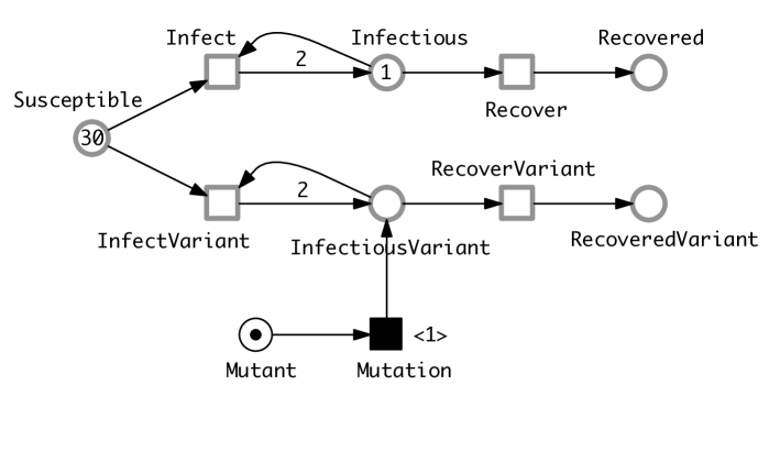
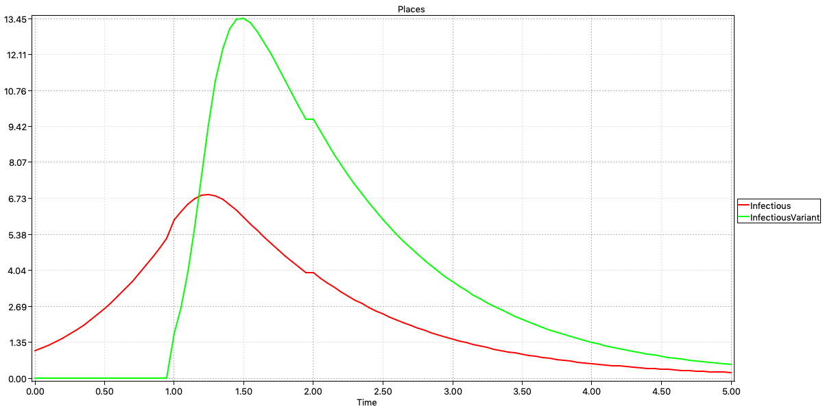
Figure C.1: SIVR model. (Top) $\mathcal{HPN}$ describing the introduction of a virus variant, using a deterministic transition Mutation which fires with a delay of 1 time unit after simulation start. Kinetic parameters: ratio between Infect and Recover, RecoverVariant is 1:10; ratio between Infect and InfectVariant is 1:5. (Bottom) Hybrid simulation trace for Infectious and InfectiousVariant.

C.2 Pandemic models

P₄SIR model, unfolded is given in Figure C.2.

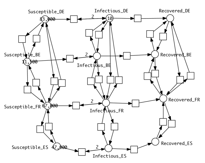
Figure C.2: P₄SIR model, unfolded obtained by unfolding P₄SIR, shown in Figure 5 (Middle), layout automatically generated.

C.3 Combined models

P₁₀SIQR model in two versions – see Figure C.3.

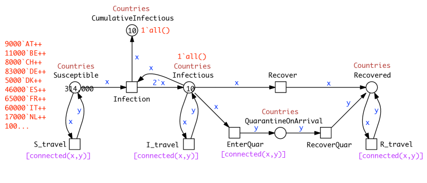
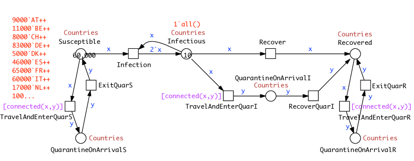
Figure C.3: P${}_{\textrm{10}}$QSIR model in two versions for West Europe (10 countries). (Top) P₁₀Q${}_{\textrm{I}}$SIR. Arrival by Infectious may possibly involve quarantine. There is an additional place CumulativeInfectious to keep a record of total infections over time. Note: this additional place destroys the conservativeness and induces a second P-invariant, comprising (all uncoloured places of) Susceptible and CumulativeInfectious. A related analysis is given in Figure C.5. (Bottom) P${}_{\textrm{10}}$QSIR. All arrivals will involve quarantine.

C.4 Parameter fitting

Parameter scanning.

Examples for varying rate parameters, see Figure C.4 for SIQR, and Figure C.5 for P₁₀Q${}_{\textrm{I}}$SIR.

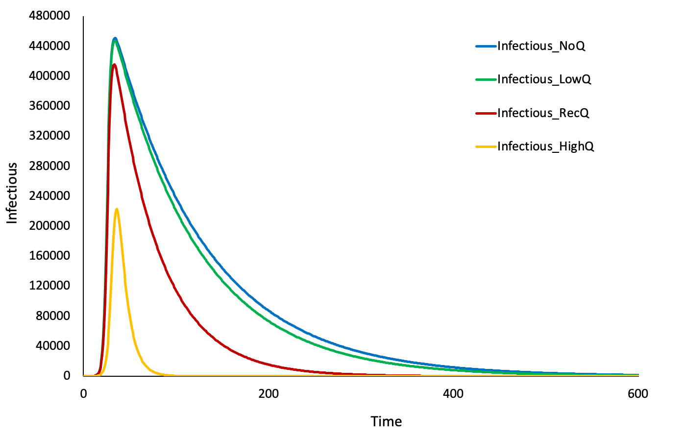
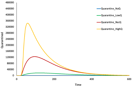
Figure C.4: SIQR model with variable quarantine rates. Four simulations of model SIQR (Figure 2 (Top)) with different Quarantine rates. NoQ = 0, LowQ = 10x less than Recover, RecQ = Recover, HighQ = 10x greater than Recover. (Top) Infectious compartment, (Bottom) Quarantined compartment.

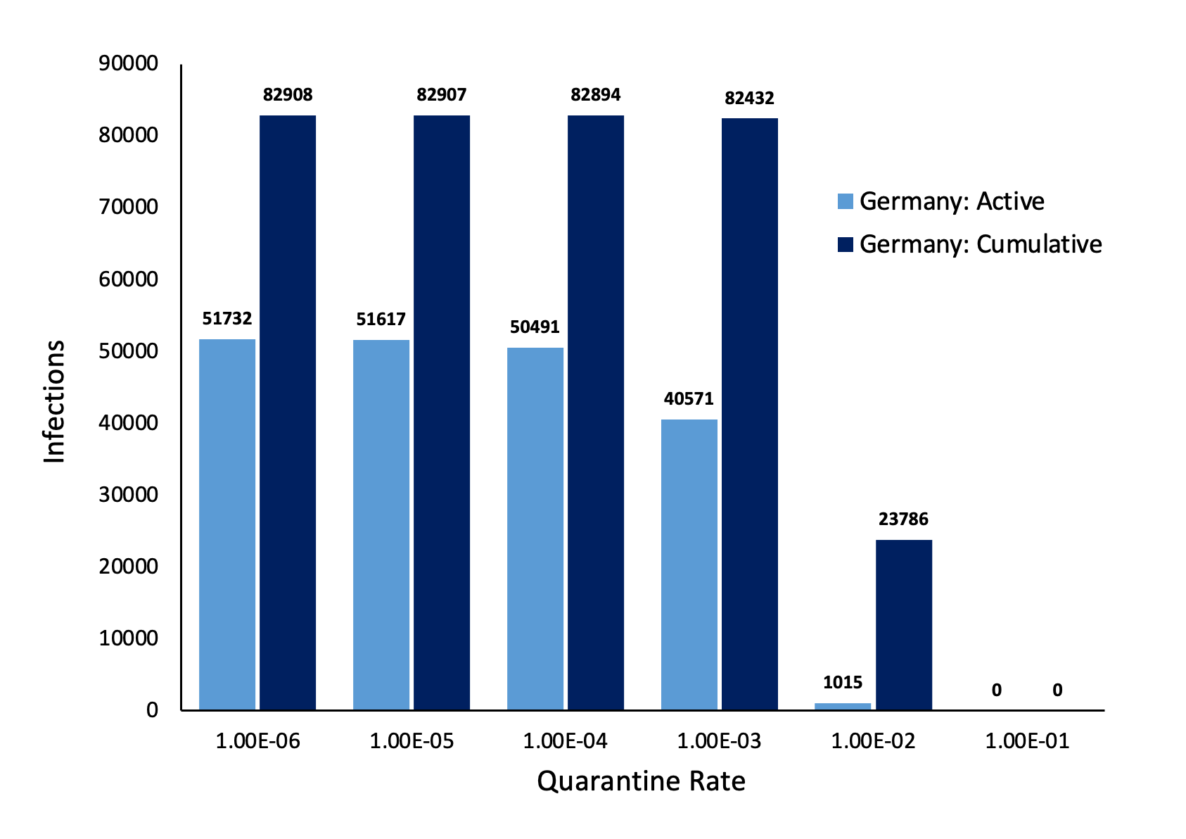
Figure C.5: P₁₀Q${}_{\textrm{I}}$SIR model – effect of modifying quarantine rates. Active and CumulativeInfectious for Germany with varying rates of Quarantine. Output from model in Figure C.3 (Top). X axis: rates for how many people go into quarantine. Y axis: Data for the peaks (active infectious at peak, cumulative at peak). Interpretation: up to a certain point quarantine only suppresses the active cases but not cumulative, lengthening out the curve, until quarantine is high.

Parameter optimisation.

The model fitted was P₁₀SIR in the unfolded version (see Figure C.6, and supplementary files P10SIR.candl, P10SIR_Separate_Rates.andl and P10SIR_Separate_Rates.cpn) employing a Random Restart Hill Climbing Algorithm (RRHCA) using real world data given in Table C.1, with results for Infection rates given in Table C.2 (Objective 1), Table C.3 (Objective 2), and Table C.4 (Objective 3). The Connection rates for Objective 3 are given in Table C.5.

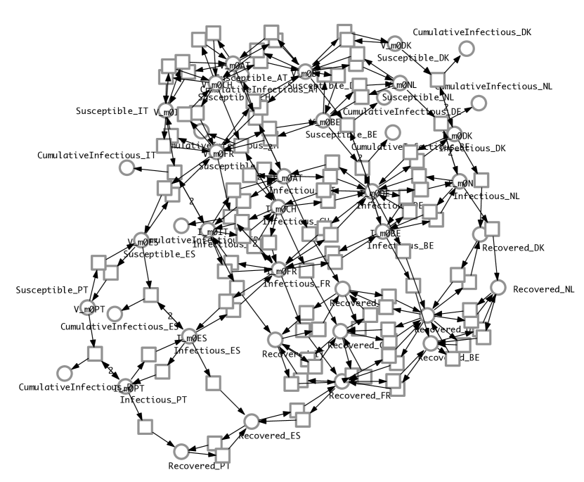
Figure C.6: P₁₀SIR model. $\mathcal{CPN}$ for SIR, West Europe, with a CumulativeInfectious place to keep a record of total infections over time; obtained by unfolding and automatic layout.

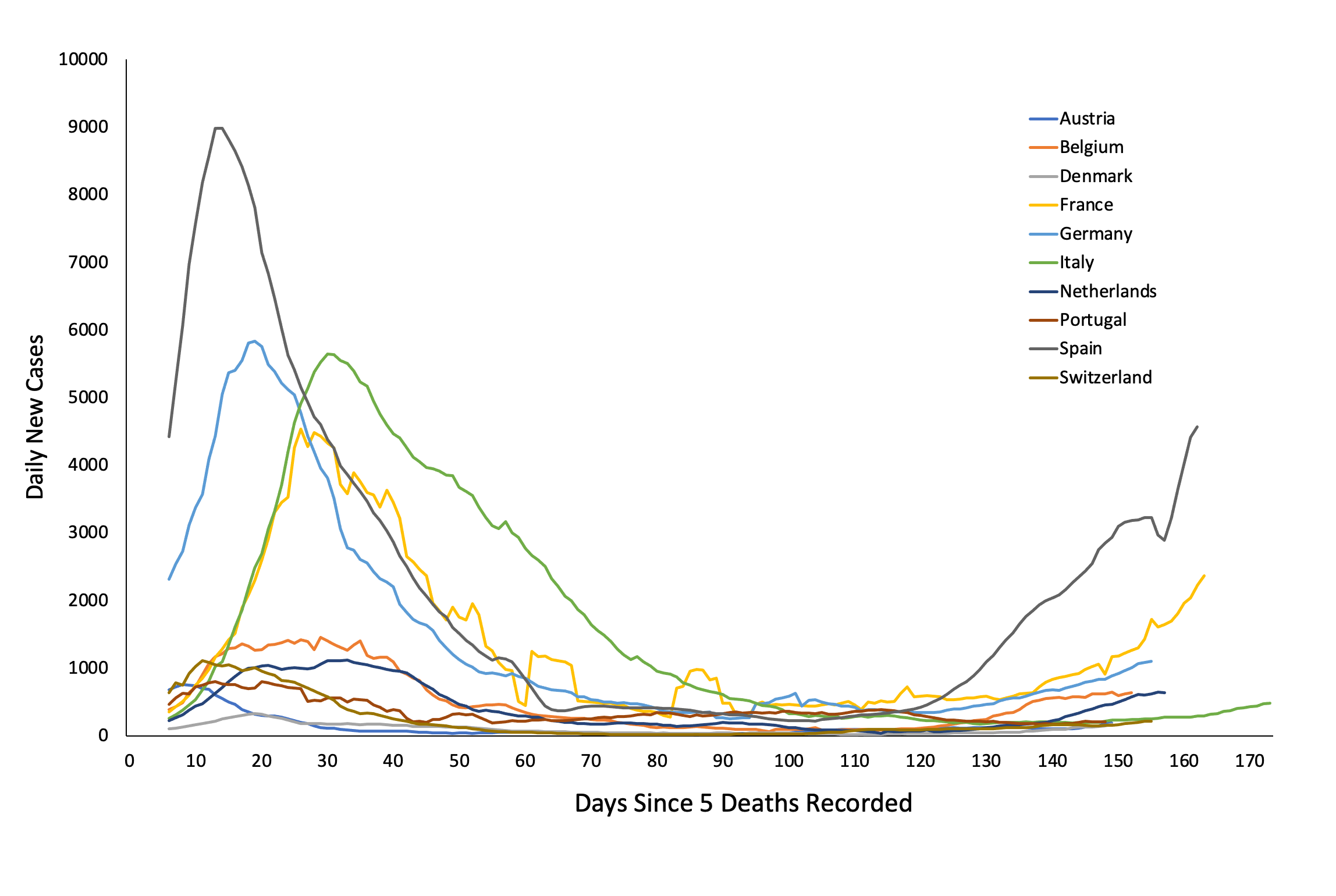
Figure C.7: Data used to fit P₁₀SIR . Real world data: daily new cases for 10 Western Europe countries, source data from WorldOmeters (https://www.worldometers.info/coronavirus/) for 19th January to 16th August 2020. Data smoothed by using a 7-day rolling average. Time: day 0 is after 5 or more cumulative deaths. Peak is the raw number. The figure shows clearer peaks for countries which reported a higher number of cases. Data used to fit the model given in Figure C.6.

Table C.1: Real world data: peak magnitude and timing of daily new cases for 10 Western Europe countries, source data from WorldOmeters (https://www.worldometers.info/coronavirus/) for 19th January to 16th August 2020.

Country	Time	Peak
Austria	8	754
Switzerland	11	1112
Portugal	13	803
Spain	14	8987
Denmark	19	328
Germany	19	5837
France	26	4537
Belgium	29	1453
Italy	30	5646
Netherlands	33	1120

Table C.2: Objective 1: Summary statistics for Random Restarts achieving the best Levenshtein Distance of 2 for model given in Figure C.6. RR = Random Restart and n refers to the number of solutions producing the summary statistics.

	Infection Rates RR0 (n=202)			Infection Rates RR5 (n=186)			Infection Rates RR9 (n=315)
Country	Mean	Min	Max	Mean	Min	Max	Mean	Min	Max
Austria	8.34e-8	3.24e-8	1.69e-7	4.05e-8	2.33e-8	6.72e-8	5.92e-7	1.69e-7	1.03e-6
Belgium	2.82e-6	2.07e-6	4.72e-6	1.98e-6	1.24e-6	3.41e-6	5.40e-7	6.68e-8	1.06e-6
Switzerland	6.72e-6	4.09e-6	1.20e-5	5.16e-7	2.64e-7	1.10e-6	1.41e-7	3.86e-9	6.89e-7
Germany	5.55e-7	3.92e-7	7.41e-7	1.98e-5	5.38e-6	3.59e-5	1.61e-6	4.88e-7	4.58e-6
Denmark	6.19e-7	1.45e-7	1.54e-6	2.93e-6	4.90e-7	9.79e-6	1.05e-7	3.51e-8	2.46e-7
Spain	2.53e-6	9.18e-7	1.00e-5	1.49e-6	8.47e-7	2.52e-6	3.83e-6	1.01e-6	9.52e-6
France	6.11e-7	4.80e-7	8.72e-7	4.83e-7	2.46e-7	7.26e-7	7.47e-7	3.44e-7	1.49e-6
Italy	4.72e-7	2.98e-7	7.00e-7	2.99e-7	2.23e-7	6.02e-7	3.45e-7	1.83e-7	5.68e-7
Netherlands	5.71e-7	3.11e-7	1.28e-6	8.31e-7	6.16e-7	1.40e-6	7.81e-7	6.10e-7	1.14e-6
Portugal	1.51e-7	5.13e-8	4.50e-7	3.35e-5	5.24e-6	8.36e-5	8.82e-5	2.63e-5	2.21e-4

Table C.3: Objective 2: Infection rates output from the best solution from the RRHCA for model given in Figure C.6. (left) Sorted alphabetically, (right) sorted by rate.

Country	Infection Rate
Austria	3.64e-5
Belgium	4.31e-5
Switzerland	3.46e-6
Germany	3.48e-6
Denmark	6.94e-6
Spain	1.80e-5
France	4.44e-6
Italy	6.57e-6
Netherlands	2.36e-6
Portugal	3.22e-5

Country	Infection Rate
Netherlands	2.36e-6
Switzerland	3.46e-6
Germany	3.48e-6
France	4.44e-6
Italy	6.57e-6
Denmark	6.94e-6
Spain	1.80e-5
Portugal	3.22e-5
Austria	3.64e-5
Belgium	4.31e-5

Table C.4: Objective 3: Infection rates output from the best solution from the RRHCA for model given in Figure C.6.(left) Sorted alphabetically, (right) sorted by rate.

Country	Infection Rate
Austria	4.05e-5
Belgium	8.03e-6
Switzerland	3.49e-5
Germany	2.89e-6
Denmark	8.69e-6
Spain	7.58e-6
France	3.75e-6
Italy	6.20e-6
Netherlands	1.11e-6
Portugal	3.49e-5

Country	Infection Rate
Netherlands	1.11e-6
Germany	2.89e-6
France	3.75e-6
Italy	6.20e-6
Spain	7.58e-6
Belgium	8.03e-6
Denmark	8.69e-6
Portugal	3.49e-5
Switzerland	3.49e-5
Austria	4.05e-5

Table C.5: Objective 3: Travel rates output from the best solution from the RRHCA for model given in Figure C.6 (Infection rates in Table C.4). Columns: Connection from; Rows: Connection to.

	AT	BE	CH	DE	DK	ES	FR	IT	NL	PT
AT			3.553e-6	1.471e-6				1.086e-5
BE				1.115e-6			5.525e-6		5.408e-7
CH	3.786e-6			1.56e-6			3.389e-7	6.361e-6
DE	3.390e-6	7.833e-6	3.443e-6		2.125e-6		4.267e-6		3.187e-6
DK				1.960e-6
ES							1.462e-6			1.565e-6
FR		1.291e-6	1.425e-6	1.082e-5		2.630e-6		7.151e-6
IT	2.535e-6		2.529e-6				1.75e-6
NL		9.549e-6		2.342e-6
PT						2.071e-5

C.5 Analysis

Visual analysis.

For an example see Figure C.8.

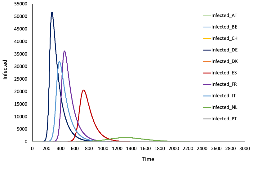
Figure C.8: P₁₀SIR behaviour. Modelled infections for 10 Western European countries connected by road. AT = Austria, BE = Belgium, CH = Switzerland, DE = Germany, DK = Denmark, ES = Spain, FR = France, IT = Italy, NL = Netherlands and PT = Portugal. Plots for countries under 100 Infected are not visible due to the scale of the graph.

Model checking

For illustration we include one experiment involving model checking, see Figure C.9.

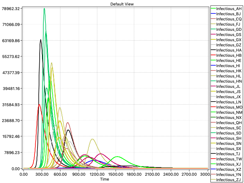
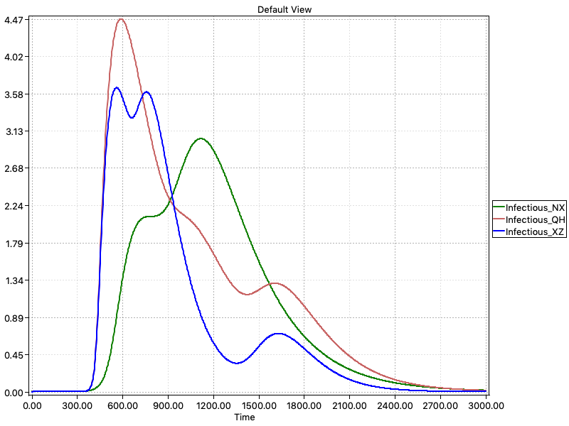
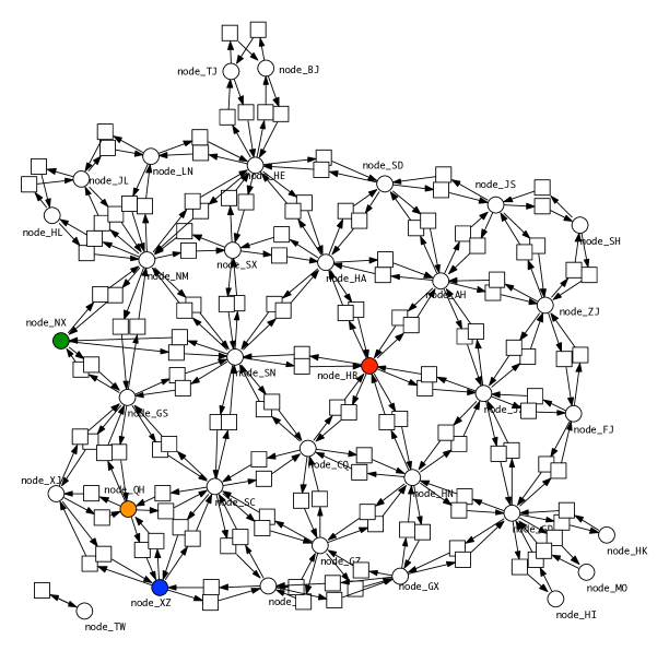
Figure C.9: P${}_{\textrm{China}}$SIR model checking. (Top, left) Time series traces of Infectious for the 34 provinces, with infection starting in Hubei. The ratio between rate constants for Infect and Recover is $1:10^{4}$ ($k_{infect}=1.0e^{-6}$, $k_{recover}=1.0e^{-2}$.) (Top, right) Model checking reveals three provinces with more than one peak. (Bottom) Network of China highlighted to indicate the geographical context of the three provinces: HB - red, NX - green, QH - brown, XZ - blue.

Correlation analysis.

Table C.6 records the variables, correlation matrices are given in Figure C.10, C.11, C.12. The correlation matrices for the unfitted models indicate that the percent of population infected at peak is related to the population size for P₄₈SIR, but not for the smaller model P₁₀SIR, perhaps because there are more smaller countries in the smaller model. The number of connections is related to the peak and peak pecentage in the larger model, but only to the peak in the smaller model. Area is a partial proxy for the whole population and is strongly related to peak and time (negatively - i.e. earlier) but not to peak percentage in P₁₀SIR. However in P₄₈SIR area is related to peak and peak percentage but not to time.

However, the correlation over the fitted data indicates that the percentage of the population at the peak is less related to the population size, compared with the unfitted model. Also the size of the peak was less related to length of time from the start of infections in the fitted model compared to the unfitted model. Finally, the time of the peak of infections was not correlated with the number of inter-country connections in the fitted model, as opposed to being negatively correlated in the unfitted model (more connections implying earlier peaks), indicating that the intervention policies that governments have taken to control the epidemic in their countries have overriden the effect of geographical connections (i.e. closing down inter-country travel).

Table C.6: Variables used to investigate road connected models further. Categories: (1) real world data external to model, (2) derived measure connecting external (black) to blue, (3) real world data incorporated in model, (4) data generated by model.

Category	Variable	Description
1	Area.Km2	Area in km2 of a given country.
2	Density	Population density of a given country (population/km2).
3	Connections	Number of connections a country has in land borders.
	initSusc	Susceptible + Infected at time 0.
	Population	The real-world country populations.
	MapPop	The population used in the model (real world population / 1000).
4	peak	The peak of Infected, this represents active cases.
	peakPerc	The percentage of initSusc that were infected at the peak.
	time	The number of steps into the simulation the peak occurred.

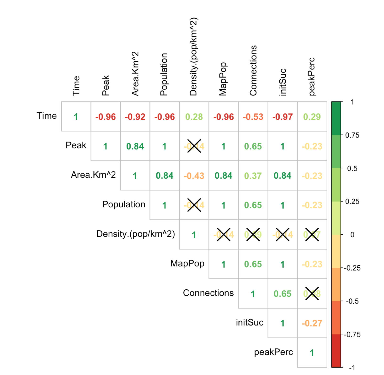
Figure C.10: Correlation matrix for P₁₀SIR, not fitted. Green indicates a strong positive correlation and red indicates a strong negative correlation. Black crosses represent a non-significant correlation. Infection rates and travel rates all identical at 1.0e^-6; recovery rates 1.0e^-2.

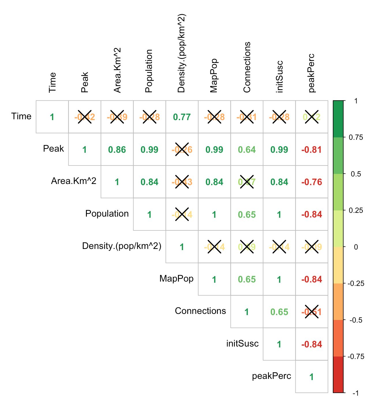
Figure C.11: Correlation matrix for P₁₀SIR, fitted. Green indicates a strong positive correlation and red indicates a strong negative correlation. Black crosses represent a non-significant correlation.

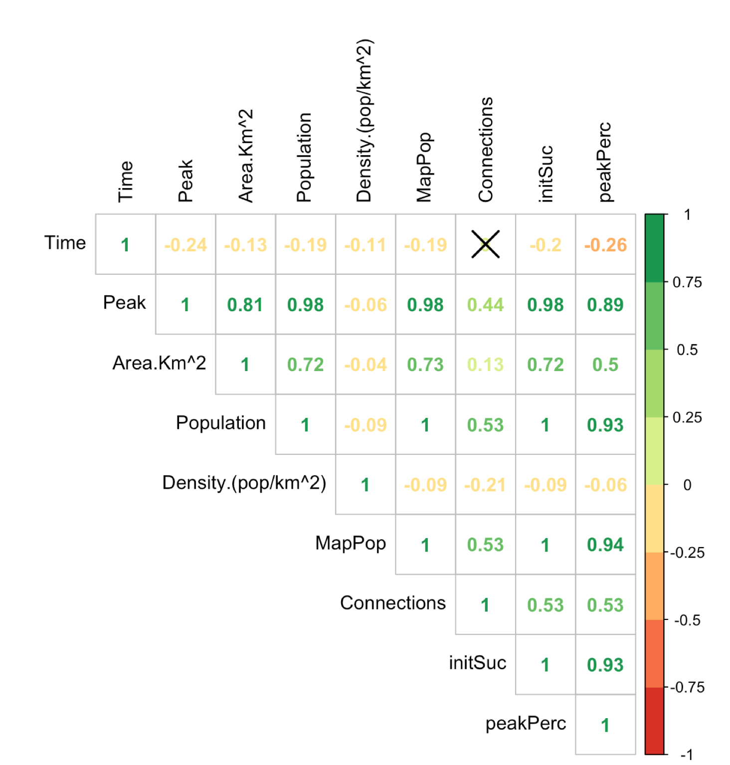
Figure C.12: Correlation matrix for P₄₈SIR, not fitted. Green indicates a strong positive correlation and red indicates a strong negative correlation. Black crosses represent a non-significant correlation.

Dendrograms.

Examples are given in Figures C.13, C.14.

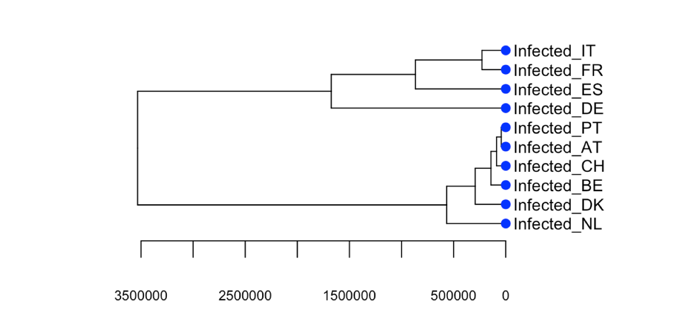
Figure C.13: Dendrogram of P₁₀SIR for West Europe, hierarchical clustering. Height is on the x-axis. Data not normalised

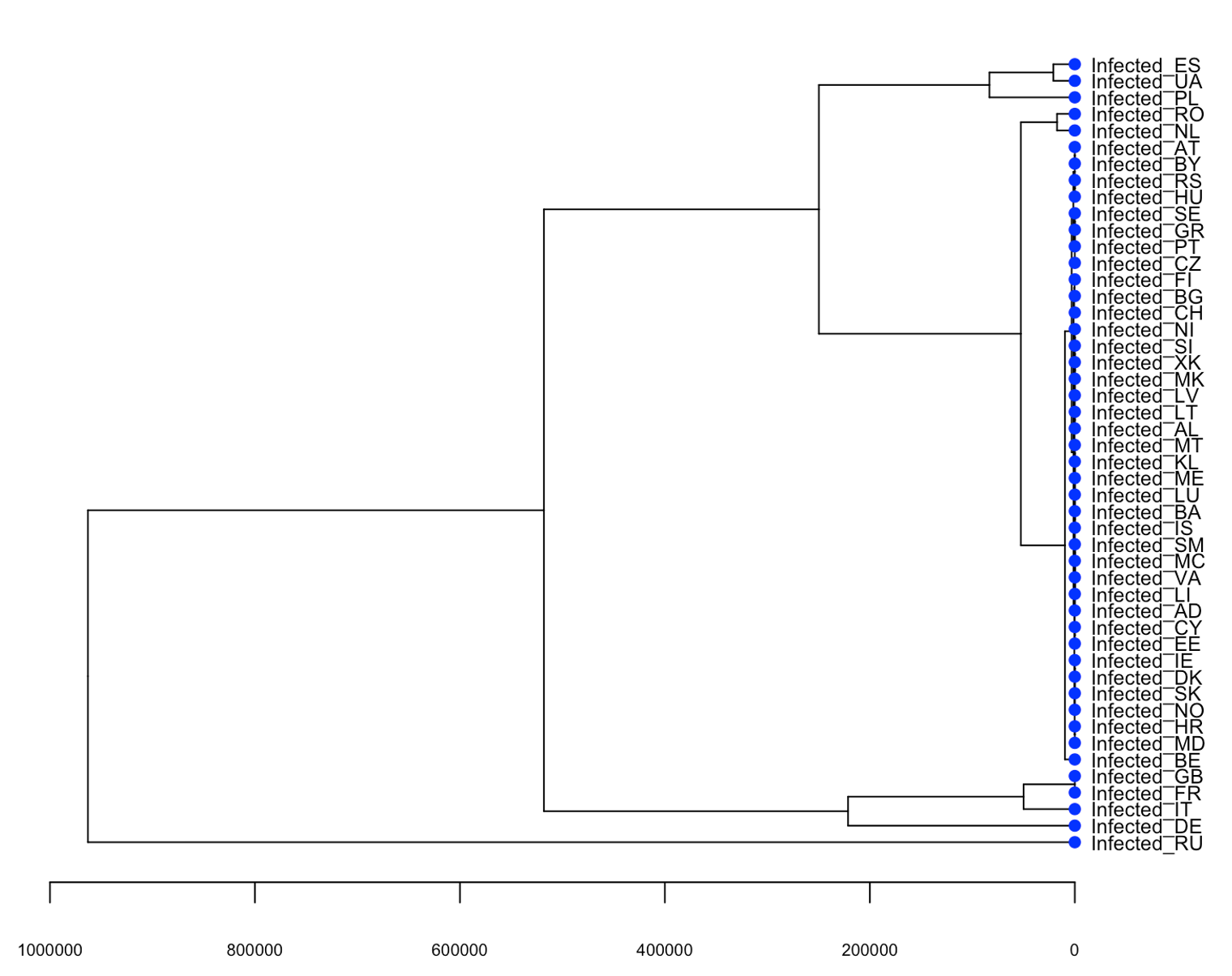
Figure C.14: Dendrogram of P₄₈SIR for Europe, hierarchical clustering. Height is on the x-axis. Data not normalised.

C.6 Discussion.

Results of simulating lockdown and unlock by dynamic change of infection rates in the SIR model; Figure C.15 - lockdown only, Figure C.16 - lockdown followed by unlock.

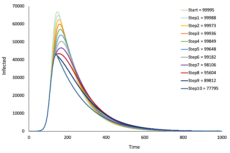
Figure C.15: SIR model - Dynamic change of infection rates: lockdown. Output from the SIR model in Figure 1 where infection rates were stepwise decremented during simulation. Figure legend shows cumulative infections for different number of decrements.

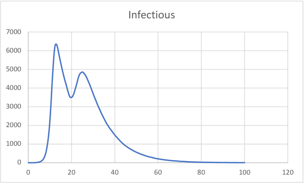
Figure C.16: SIR model, dynamic change of infection rate increased back to pre-intervention level at time step 20.

Appendix D List of Files Provided

All models given in figures (provided as Snoopy files):

• SIR.spn - standard SIR, see Figure 1

• SIQR.spn - SIR extended by quarantine, see Figure 2 (Top)

• SIAR.spn - SIR extend by symptomatic/asymptomatic compartments, see Figure 2 (Bottom)

• SIR-S2.spn - SIR-S${}_{2}^{age}$, uncoloured, see Figure 3 (Top)

• SIR-S2_enum.colspn, SIR-S2_int.colspn - SIR-S${}_{2}^{age}$, coloured, see Figure 3 (Middle)

• SIR-S20.spn - SIR-S₂₀, see Figure 3 (Bottom)

• P2-SIR.spn - P₂SIR, uncoloured, see Figure 4 (Top)

• P2-SIR.colspn - P₂SIR, coloured, see Figure 4 (Bottom)

• network-Europe4.spn - connectivity graph for Europe, 4 countries, uncoloured, see Figure 5 (Top middle)

• network-Europe4.colspn - connectivity graph for Europe, 4 countries, coloured, see Figure 5 (Top right)

• P4-SIR.colspn - P₄SIR, coloured, see Figure 5 (Middle)

• P4-SIR.spn - P₄SIR, uncoloured, see Figure C.2

• P48-SIR-S10.colspn - P₄₈SIR-S₁₀, see Figure 5 (Bottom)

• P48-SIR-S10.andl.spn - P₄₈SIR-S₁₀ unfolded, see Figure 6 (Bottom)

• SIVR.hpn - SIR with variant virus, see FigureC.1

• P10-QI-SIR.colspn - P₁₀Q$\_\textrm{I}$SIR, see Figure C.3 (Top)

• P10-QSIR.colspn - P₁₀QSIR, see Figure C.3 (Bottom)

• P10-SIR_Separate_Rates.cpn - $\mathcal{CPN}$ used for parameter optimisation - unfolded version of P₁₀SIR, given in Figure C.6.

Connectivity networks (provided as CANDL files):

• network-Europe04.candl
  - unfolding: |P|=4, |T|=8, |A|=16

• network-Europe05.candl
  - unfolding: |P|=5, |T|=16, |A|=32

• network-Europe10.candl
  - unfolding: |P|=10, |T|=30, |A|=60

• network-Europe48.candl
  - unfolding: |P|=47, |T|=170, |A|=340
  - note: IS isolated, https://countrycode.org
  - unfolding time: 1.302sec

• network-China.candl
  - unfolding: P|=33, |T|=142, |A|=286
  - note: 34 states; TW isolated
  - unfolding time: 0.283sec

• network-USA.candl
  - unfolding: |P|=48, |T|=210, |A|=420
  - note: 50 states; AK, HI isolated
  - unfolding time: 1.643sec

P_nSIR models (provided as CANDL files):

• P-Europe02-SIR - Europe fragment, 2 countries

• P-Europe04-SIR - Europe fragment, 4 countries

• P-Europe10-SIR - Western Europe, 10 countries

• P-Europe48-SIR - All Europe, 48 countries

• P-China-SIR - China, 34 provinces

• P-USA-SIR - USA, 50 states

Python programs:

• RRHCA (Random Restart Hill Climbing)

• Python Web Scraper, used to to collect COVID19 Data.

R code:

• Europe.Rmd, Western_Europe.Rmd: Both these files take in csv outputs from Snoopy, Spike to produce correlation matrices and regression analysis. The Time and Infectious traces are extracted from the csv files and joined to real world data (e.g. population, density, country size). Correlation matrices are then produced. Regression analysis is also conducted along with checking the assumptions of regression.

• Clustering.Rmd: This code takes in one csv file (output from Snoopy, Spike) and performs agglomerative hierarchical clustering using Euclidean distance and complete-linkage. This code selects Time and Infected traces to perform the clustering. The code plots a dendrogram of the clustering results for visualisation.

Spike:

• config file + andl/candl file

• all source files to produce Figure C.16.

MC2:

• property library and Unix script to produce Figure C.9.

References

- [ABCC+20] Francesc Aràndiga, Antonio Baeza, Isabel Cordero-Carrión, Rosa Donat, M Carmen Martí, Pep Mulet, and Dionisio F Yáñez. A Spatial-Temporal Model for the Evolution of the COVID-19 Pandemic in Spain Including Mobility. Mathematics, 8(10):1677, 2020.
- [ACR+21] George Assaf, Jacek Chodak, Christian Rohr, Martin Schwarick, and Monika Heiner. CANDL Report. Technical report, Brandenburg University of Technology Cottbus, Department of Computer Science, 2021. to appear.
- [Ada20] David Adam. A guide to R — the pandemic’s misunderstood metric. Nature, 583(7816):346–348, 2020.
- [AHL19] George Assaf, Monika Heiner, and Fei Liu. Biochemical reaction networks with fuzzy kinetic parameters in Snoopy. In L Bortolussi and G Sanguinetti, editors, Proc. CMSB 2019, volume 11773 of LNCS/LNBI, pages 302–307. Springer, September 2019. First Online: 17 September 2019.
- [ASGS20] Nikhil Anand, A Sabarinath, S Geetha, and S Somanath. Predicting the spread of covid-19 using sir model augmented to incorporate quarantine and testing. Transactions of the Indian National Academy of Engineering, 5(2):141–148, 2020.
- [BCG+09] Duygu Balcan, Vittoria Colizza, Bruno Gonçalves, Hao Hu, José J Ramasco, and Alessandro Vespignani. Multiscale mobility networks and the spatial spreading of infectious diseases. Proceedings of the National Academy of Sciences, 106(51):21484–21489, 2009.
- [BFF+15] Marco Beccuti, Chiara Fornari, Giuliana Franceschinis, Sami M Halawani, Omar Ba-Rukab, Ab Rahman Ahmad, and Gianfranco Balbo. From symmetric nets to differential equations exploiting model symmetries. The Computer Journal, 58(1):23–39, 2015.
- [BGH+10] Duygu Balcan, Bruno Gonçalves, Hao Hu, José J Ramasco, Vittoria Colizza, and Alessandro Vespignani. Modeling the spatial spread of infectious diseases: The GLobal Epidemic and Mobility computational model. Journal of computational science, 1(3):132–145, 2010.
- [BGHO08] Rainer Breitling, David Gilbert, Monika Heiner, and Richard Orton. A structured approach for the engineering of biochemical network models, illustrated for signalling pathways. Briefings in Bioinformatics, 9(5):404–421, September 2008.
- [BHM15] Mary-Ann Blätke, Monika Heiner, and Wolfgang Marwan. BioModel Engineering with Petri Nets, chapter 7, pages 141–193. Elsevier Inc., March 2015.
- [BM20] Fadoua Balabdaoui and Dirk Mohr. Age-stratified model of the COVID-19 epidemic to analyze the impact of relaxing lockdown measures: nowcasting and forecasting for Switzerland. medRxiv, 2020.
- [BPR+11] Paolo Bajardi, Chiara Poletto, Jose J Ramasco, Michele Tizzoni, Vittoria Colizza, and Alessandro Vespignani. Human mobility networks, travel restrictions, and the global spread of 2009 H1N1 pandemic. PloS one, 6(1):e16591, 2011.
- [Bra17] Fred Brauer. Mathematical epidemiology: Past, present, and future. Infectious Disease Modelling, 2(2):113–127, 2017.
- [CH19] Jacek Chodak and Monika Heiner. Spike – reproducible simulation experiments with configuration file branching. In L Bortolussi and G Sanguinetti, editors, Proc. CMSB 2019, volume 11773 of LNCS/LNBI, pages 315–321. Springer, September 2019.
- [CPG+20] Paolo Castagno, Simone Pernice, Gianni Ghetti, Massimiliano Povero, Lorenzo Pradelli, Daniela Paolotti, Gianfranco Balbo, Matteo Sereno, and Marco Beccuti. A computational framework for modeling and studying pertussis epidemiology and vaccination. BMC bioinformatics, 21(8):1–32, 2020.
- [CTTV17] Luca Cardelli, Mirco Tribastone, Max Tschaikowski, and Andrea Vandin. ERODE: A Tool for the Evaluation and Reduction of Ordinary Differential Equations. In TACAS 2017, pages 310–328. Springer, LNCS 10206, 2017.
- [CV08] Vittoria Colizza and Alessandro Vespignani. Epidemic modeling in metapopulation systems with heterogeneous coupling pattern: Theory and simulations. Journal of theoretical biology, 251(3):450–467, 2008.
- [CYX14] Yao Chen, Mei Yan, and Zhongyi Xiang. Transmission dynamics of a two-city SIR epidemic model with transport-related infections. Journal of Applied Mathematics, 2014, 2014.
- [DG08] Ronald Donaldson and David Gilbert. A model checking approach to the parameter estimation of biochemical pathways. In Proc. CMSB, pages 269–287. LNCS 5307, Springer, 2008.
- [DVHC13] Sara Y Del Valle, James M Hyman, and Nakul Chitnis. Mathematical models of mixing patterns between age groups for predicting the spread of infectious diseases. Math. Biosci. Eng, 20:1–20, 2013.
- [EDK10] Stefan B Edlund, Matthew A Davis, and James H Kaufman. The spatiotemporal epidemiological modeler. In Proceedings of the 1st ACM International Health Informatics Symposium, pages 817–820, 2010.
- [Fra09] Andreas Franzke. Charlie 2.0 – a multi-threaded Petri net analyzer. Diploma thesis, Brandenburg University of Technology Cottbus, Department of Computer Science, December 2009.
- [GBB+20] Giulia Giordano, Franco Blanchini, Raffaele Bruno, Patrizio Colaneri, Alessandro Di Filippo, Angela Di Matteo, and Marta Colaneri. Modelling the COVID-19 epidemic and implementation of population-wide interventions in Italy. Nature Medicine, pages 1–6, 2020.
- [GGH+13] Qian Gao, David Gilbert, Monika Heiner, Fei Liu, Daniele Maccagnola, and David Tree. Multiscale Modelling and Analysis of Planar Cell Polarity in the Drosophila Wing. IEEE/ACM Transactions on Computational Biology and Bioinformatics, 10(2):337–351, 2013.
- [GHGC19] David Gilbert, Monika Heiner, Leila Ghanbar, and Jacek Chodak. Spatial quorum sensing modelling using coloured hybrid Petri nets and simulative model checking. BMC Bioinformatics, 20(supplement 4), 2019.
- [GHLS13] David Gilbert, Monika Heiner, Fei Liu, and Nigel Saunders. Colouring Space - A Coloured Framework for Spatial Modelling in Systems Biology. In JM Colom and J Desel, editors, Proc. PETRI NETS 2013, volume 7927 of LNCS, pages 230–249. Springer, June 2013.
- [Gil76] Daniel T Gillespie. A General Method for Numerically Simulating the Stochastic Time Evolution of Coupled Chemical Species. J. of Computational Physics, 22:403–434, 1976.
- [GL81] Hartmann J Genrich and Kurt Lautenbach. System modelling with high-level Petri nets. Theoretical computer science, 13(1):109–135, 1981.
- [GMW20] Guojun Gan, Chaoqun Ma, and Jianhong Wu. Data clustering: theory, algorithms, and applications. SIAM, 2020.
- [GS20] Rahul Goel and Rajesh Sharma. Mobility Based SIR Model For Pandemics–With Case Study Of COVID-19. arXiv preprint arXiv:2004.13015, 2020.
- [HBG+05] Alan C Hindmarsh, Peter N Brown, Keith E Grant, Steven L Lee, Radu Serban, Dan E Shumaker, and Carol S Woodward. Sundials: Suite of nonlinear and differential/algebraic equation solvers. ACM Trans. Math. Softw., 31:363–396, 2005.
- [Hei09] Monika Heiner. Understanding Network Behaviour by Structured Representations of Transition Invariants – A Petri Net Perspective on Systems and Synthetic Biology, pages 367–389. Natural Computing Series. Springer, 2009.
- [Het00] Herbert W Hethcote. The mathematics of infectious diseases. SIAM review, 42(4):599–653, 2000.
- [HG11] Monika Heiner and David Gilbert. How Might Petri Nets Enhance Your Systems Biology Toolkit, volume 6709 of Lecture Notes in Computer Science, pages 17–37. Springer, 2011.
- [HG13] Monika Heiner and David Gilbert. Biomodel engineering for multiscale systems biology. Progress in Biophysics and Molecular Biology, 111(2-3):119–128, April 2013. online available 12-OCT-2012.
- [HGD08] Monika Heiner, David Gilbert, and Ronald Donaldson. Petri Nets for Systems and Synthetic Biology, volume 5016 of LNCS, pages 215–264. Springer, 2008.
- [HHL+12] Monika Heiner, Mostafa Herajy, Fei Liu, Christian Rohr, and Martin Schwarick. Snoopy - a unifying Petri net tool. In Proc. PETRI NETS 2012, volume 7347 of LNCS, pages 398–407. Springer, June 2012.
- [HLRH17] Mostafa Herajy, Fei Liu, Christian Rohr, and Monika Heiner. Coloured Hybrid Petri Nets in Snoopy - User Manual. Technical Report 01-17, Brandenburg University of Technology Cottbus, Department of Computer Science, March 2017.
- [HRS13] Monika Heiner, Christian Rohr, and Martin Schwarick. MARCIE - Model checking And Reachability analysis done effiCIEntly. In JM Colom and J Desel, editors, Proc. PETRI NETS 2013, volume 7927 of LNCS, pages 389–399. Springer, June 2013.
- [HRSS10] Monika Heiner, Christian Rohr, Martin Schwarick, and Stefan Streif. A comparative study of stochastic analysis techniques. In Proc. 8th International Conference on Computational Methods in Systems Biology (CMSB 2010), pages 96–106. ACM digital library, September 2010.
- [HRST16] M Heiner, C Rohr, M Schwarick, and A Tovchigrechko. MARCIE’s secrets of efficient model checking. Transactions on Petri Nets and Other Models of Concurrency (ToPNoC) XI, LNCS 9930, pages 286–296, 2016.
- [HSW05] Jane M Heffernan, Robert J Smith, and Lindi M Wahl. Perspectives on the basic reproductive ratio. Journal of the Royal Society Interface, 2(4):281–293, 2005.
- [HSW15] Monika Heiner, Martin Schwarick, and Jahn Wegener. Charlie - an extensible Petri net analysis tool. In R Devillers and A Valmari, editors, Proc. PETRI NETS 2015, volume 9115 of LNCS, pages 200–211. Springer, June 2015.
- [IHAH20] Amr Ismail, Mostafa Herajy, Elsayed Atlam, and Monika Heiner. A Graphical Approach for Hybrid Simulation of 3D Diffusion Bio-models via Coloured Hybrid Petri Nets. Modelling and Simulation in Engineering, 2020. Article ID 4715172, 14 pages.
- [JK09] Kurt Jensen and Lars M Kristensen. Coloured Petri nets: modelling and validation of concurrent systems. Springer, 2009.
- [Lev66] Vladimir I Levenshtein. Binary codes capable of correcting deletions, insertions, and reversals. In Soviet physics doklady, volume 10, pages 707–710, 1966.
- [LHG19] Fei Liu, Monika Heiner, and David Gilbert. Coloured Petri nets for multilevel, multiscale, and multidimensional modelling of biological systems. Briefings in Bioinformatics, 20(3):877–886, 2019. Published: 03 November 2017.
- [LHR12] Fei Liu, Monika Heiner, and Christian Rohr. The Manual for Colored Petri Nets in Snoopy – ///. Technical Report 02-12, BTU Cottbus, Dep. of CS, 2012.
- [LJ88] Ira M Longini Jr. A mathematical model for predicting the geographic spread of new infectious agents. Mathematical Biosciences, 90(1-2):367–383, 1988.
- [MAS+20] Imran Mahmood, Hamid Arabnejad, Diana Suleimenova, Isabel Sassoon, Alaa Marshan, Alan Serrano-Rico, Panos Louvieris, Anastasia Anagnostou, Simon J E Taylor, David Bell, and Derek Groen. FACS: a geospatial agent-based simulator for analysing COVID-19 spread and public health measures on local regions. Journal of Simulation, 0(0):1–19, 2020.
- [MRH12] Wolfgang Marwan, Christian Rohr, and Monika Heiner. Petri nets in Snoopy: A unifying framework for the graphical display, computational modelling, and simulation of bacterial regulatory networks, volume 804 of Methods in Molecular Biology, chapter 21, pages 409–437. Humana Press, 2012.
- [Mur89] Tadao Murata. Petri nets: Properties, analysis and applications. Proceedings of the IEEE, 77(4):541–580, 1989.
- [NA19] Aadrita Nandi and Linda JS Allen. Stochastic two-group models with transmission dependent on host infectivity or susceptibility. Journal of Biological Dynamics, 13(sup1):201–224, 2019.
- [OWZ20] Tatsushi Oka, Wei Wei, and Dan Zhu. A Spatial Stochastic SIR Model for Transmission Networks with Application to COVID-19 Epidemic in China. SSRN, 2020.
- [PGH+15] Ovidiu Pârvu, David Gilbert, Monika Heiner, Fei Liu, Nigel Saunders, and Simon Shaw. Spatial-temporal modelling and analysis of bacterial colonies with phase variable genes. ACM Transactions on Modeling and Computer Simulation (TOMACS), 25(2):25p., May 2015.
- [PLR+20] Kiesha Prem, Yang Liu, Timothy W Russell, Adam J Kucharski, Rosalind M Eggo, Nicholas Davies, Stefan Flasche, Samuel Clifford, Carl AB Pearson, James D Munday, et al. The effect of control strategies to reduce social mixing on outcomes of the COVID-19 epidemic in Wuhan, China: a modelling study. The Lancet Public Health, 2020.
- [RLJ85] Leonid A Rvachev and Ira M Longini Jr. A mathematical model for the global spread of influenza. Mathematical biosciences, 75(1):3–22, 1985.
- [RN13] Stuart Russell and Peter Norvig. Artificial intelligence: Pearson new international edition: A modern approach. Pearson Higher Ed, 2013.
- [SD95] Lisa Sattenspiel and Klaus Dietz. A structured epidemic model incorporating geographic mobility among regions. Mathematical Biosciences, 128(1):71–92, 1995.
- [SH09] Martin Schwarick and Monika Heiner. CSL model checking of biochemical networks with interval decision diagrams. In Proc. 7th International Conference on Computational Methods in Systems Biology (CMSB 2009), volume 5688 of LNCS/LNBI, pages 296–312. Springer, September 2009.
- [SH10] Sylvain Soliman and Monika Heiner. A unique transformation from ordinary differential equations to reaction networks. PLoS ONE, 5(12):e14284, 2010.
- [SIAQN17] De la Manuel Sen, Asier Ibeas, Santiago Alonso-Quesada, and Raul Nistal. On a new epidemic model with asymptomatic and dead-infective subpopulations with feedback controls useful for Ebola disease. Discrete dynamics in Nature and society, 2017.
- [SP93] Lisa Sattenspiel and Christopher Powell. Geographic spread of measles on the island of Dominica, West Indies. Human biology, pages 107–129, 1993.
- [SRH16] M Schwarick, C Rohr, and M Heiner. MARCIE Manual. Technical Report 02-16, Brandenburg University of Technology Cottbus, Department of Computer Science, December 2016.
- [SRL+20] Martin Schwarick, Christian Rohr, Fei Liu, Georgea Assaf, Jacek Chodak, and Monika Heiner. Efficient Unfolding of Coloured Petri Nets using Interval Decision Diagrams. In T Chatain R Janicki, N Sidorova, editor, Proc. PETRI NETS 2020, volume 12152 of LNCS, pages 324–344. Springer, Cham, June 2020.
- [VdBGG+11] Wouter Van den Broeck, Corrado Gioannini, Bruno Gonçalves, Marco Quaggiotto, Vittoria Colizza, and Alessandro Vespignani. The GLEaMviz computational tool, a publicly available software to explore realistic epidemic spreading scenarios at the global scale. BMC infectious diseases, 11(1):1–14, 2011.
- [vdD17] Pauline van den Driessche. Reproduction numbers of infectious disease models. Infectious Disease Modelling, 2(3):288–303, 2017.
- [WW45] Edwin B Wilson and Jane Worcester. The law of mass action in epidemiology. Proceedings of the National Academy of Sciences of the United States of America, 31(1):24, 1945.
- [WxW21] Wxwidgets website. http://www.wxwidgets.org, 2021. Accessed: 20/3/2021.