Quantifying Availability and Discovery in Recommender Systems via Stochastic Reachability

Abstract

In this work, we consider how preference models in interactive recommendation systems determine the availability of content and users’ opportunities for discovery. We propose an evaluation procedure based on stochastic reachability to quantify the maximum probability of recommending a target piece of content to an user for a set of allowable strategic modifications. This framework allows us to compute an upper bound on the likelihood of recommendation with minimal assumptions about user behavior. Stochastic reachability can be used to detect biases in the availability of content and diagnose limitations in the opportunities for discovery granted to users. We show that this metric can be computed efficiently as a convex program for a variety of practical settings, and further argue that reachability is not inherently at odds with accuracy. We demonstrate evaluations of recommendation algorithms trained on large datasets of explicit and implicit ratings. Our results illustrate how preference models, selection rules, and user interventions impact reachability and how these effects can be distributed unevenly.

1 Introduction

Through recommendation systems, personalized preference models mediate access to many types of information on the internet. Aiming to surface content that will be consumed, enjoyed, and highly rated, these models are primarily designed to accurately predict individuals’ preferences. However, it is important to look beyond measures of accuracy towards notions of access. The focus on improving recommender model accuracy favors systems in which human behavior becomes as predictable as possible—effects which have been implicated in unintended consequences like polarization or radicalization.

We focus on questions of access and agency by adopting an interventional lens, which considers arbitrary and strategic user actions. We expand upon the notion of reachability first proposed by Dean et al. (2020), which measures the ability of an individual to influence a recommender model to select a certain piece of content. We define a notion of stochastic reachability which quantifies the maximum achievable likelihood of a given recommendation in the presence of strategic interventions. This metric provides an upper bound on the ability of individuals to discover specific content, thus isolating unavoidable biases within preference models from those due to user behavior.

Our primary contribution is the definition of metrics based on stochastic reachability which capture the possible outcomes of a round of system interactions, including the availability of content and discovery possibilities for individuals. In Section 3, we show that they can be computed by solving a convex optimization problem for a class of relevant recommenders. In Section 4, we draw connections between the stochastic and deterministic settings. This perspective allows us to describe the relationship between agency and stochasticity and further to argue that there is not an inherent trade-off between reachability and model accuracy. Finally, we present an audit of recommendation systems using a variety of datasets and preference models. We explore how design decisions influence reachability and the extent to which biases in the training datasets are propagated.

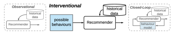
Figure 1: Conceptual framings of recommendation systems consider user behaviors to varying degrees. In this work we focus on evaluating interventional properties.

1.1 Related Work

The recommender systems literature has long proposed a variety of other metrics for evaluation, including notions of novelty, serendipity, diversity, and coverage Herlocker et al. (2004); Castells et al. (2011). There is a long history of measuring and mitigating bias in recommendation systems Chen et al. (2020). Empirical investigations have found evidence of popularity and demographic bias in domains including movies, music, books, and hotels Abdollahpouri et al. (2019); Ekstrand et al. (2018a, b); Jannach et al. (2015). Alternative metrics are useful both for diagnosing biases and as objectives for post-hoc mitigating techniques such as calibration Steck (2018) and re-ranking Singh and Joachims (2018). A inherent limitation of these approaches is that they focus on observational bias induced by preference models, i.e. examining the result of a single round of recommendations without considering individuals’ behaviors. While certainly useful, they fall short of providing further understanding into the interactive nature of recommendation systems.

The behavior of recommendation systems over time and in closed-loop is still an open area of study. It is difficult to definitively link observational evidence of radicalization Ribeiro et al. (2020); Faddoul et al. (2020) to proprietary recommendation algorithms. Empirical studies of human behavior find mixed results on the relationship between recommendation and content diversity Nguyen et al. (2014); Flaxman et al. (2016). Simulation studies Chaney et al. (2018); Yao et al. (2021); Krauth et al. (2020) and theoretical investigations Dandekar et al. (2013) shed light on phenomena in simplified settings, showing how homogenization, popularity bias, performance, and polarization depend on assumed user behavior models. Even ensuring accuracy in sequential dynamic settings requires contending with closed-loop behaviors. Recommendation algorithms must mitigate biased sampling in order to learn underlying user preference models, using causal inference based techniques Schnabel et al. (2016); Yang et al. (2018) or by balancing exploitation and exploration Kawale et al. (2015); Mary et al. (2015). Reinforcement Learning algorithms contend with these challenges while considering a longer time horizon Chen et al. (2019); Ie et al. (2019), implicitly using data to exploit user behavior.

Our work eschews behavior models in favor of an interventional framing which considers a variety of possible user actions. Giving users control over their recommendations has been found to have positive effects, while reducing agency has negative effects Harper et al. (2015); Lukoff et al. (2021). The formal perspective we take on agency and access in recommender systems was first introduced by Dean et al. (2020), and is closely related to a body on work on recourse in consequential decision making Ustun et al. (2019); Karimi et al. (2020). We build on this work to consider stochastic recommendation policies.

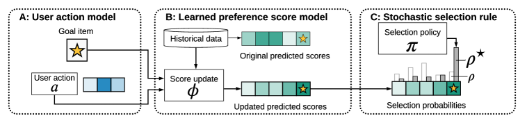
Figure 2: We audit recommender systems under a user action model (A), learned preference model (B), and stochastic selection rule (C).

2 Metrics Based on Reachability

2.1 Stochastic Recommender Setting

We consider systems composed of $n$ individuals as well as a collection of $m$ pieces of content. For consistency with the recommender systems literature, we refer to individuals as users, pieces of content as items, and expressed preferences as ratings. We will denote a rating by user $u$ of item $i$ as $r_{ui}\in\mathcal{R}$, where $\mathcal{R}\subseteq\mathbb{R}$ denotes the space of values which ratings can take. For example, ratings corresponding to the percentage of a video watched would have $\mathcal{R}=[0,1]$ while discrete star ratings would have $\mathcal{R}=\{1,2,3,4,5\}$. The number of observed ratings will generally be much smaller than the total number of possible ratings, and we denote by $\Omega_{u}\subseteq\{1,\dots,m\}$ the set of items seen by the user $u$. The goal of a recommendation system is to understand the preferences of users and recommend relevant content.

In this work, we focus on the common setting in which recommenders are the composition of a scoring function $\phi$ with selection rule $\pi$ (Figure 2). The scoring function models the preferences of users. It is constructed based on historical data (e.g. observed ratings, user/item features) and returns a score for each user and item pair. For a given user $u$ and item $i$, we denote $s_{ui}\in\mathbb{R}$ to be the associated score, and for user $u$ we will denote by $\mathbf{s}_{u}\in\mathbb{R}^{m}$ the vector of scores for all items. A common example of a scoring function is a machine learning model which predicts future ratings based on historical data.

We will focus on the way that scores are updated after a round of user interaction. For example, if a user consumes and rates several new items, the recommender system should update the scores in response. Therefore, we parameterize the score function by an update rule, so that the new score vector is $\mathbf{s}_{u}^{+}=\phi_{u}(\mathbf{a})$, where $\mathbf{a}\in\mathcal{A}_{u}$ represents actions taken by user $u$ and $\mathcal{A}_{u}$ represents the set of all possible actions. Thus $\phi_{u}$ encodes the historical data, the preference model class, and the update algorithm. The action space $\mathcal{A}_{u}$ represents possibilities for system interaction, encoding for example limitations due to user interface design. We define the form of the score update function and discuss the action space in more detail in Section 3.

The selection rule $\pi$ is a policy which, for given user $u$ and scores $\mathbf{s}_{u}$, selects one or more items from a set of specified target items $\Omega_{u}^{t}\subseteq\{1,\dots,m\}$ as the next recommendation. The simplest selection rule is a top-1 policy, which is a deterministic rule that selects the item with the highest score for each user. A simple stochastic rule is the $\epsilon$-greedy policy which with probability $1-\epsilon$ selects the top scoring item and with probability $\epsilon$ chooses uniformly from the remaining items. Many additional approaches to recommendation can be viewed as the composition of a score function with a selection policy. This setting also encompasses implicit feedback scenarios, where clicks or other behaviors are defined as or aggregated into “ratings.” Many recommendation algorithms, even those not specifically motivated by regression, include an intermediate score prediction step, e.g. point-wise approaches to ranking. Further assumptions in Section 3 will not capture the full complexity of other techniques such as pairwise ranking and slate-based recommendations. We leave such extensions to future work.

In this work, we are primarily interested in stochastic policies which select items according to a probability distribution on the scores $\mathbf{s}_{u}$ parametrized by a exploration parameter. Policies of this form are often used to balance exploration and exploration in online or sequential learning settings. A stochastic selection rule recommends an item $i$ according to $\mathbb{P}\left(\pi(\mathbf{s}_{u},\Omega^{t}_{u})=i\right)$, which is 0 for all non-target items $i\notin\Omega_{u}^{t}$. For example, to select among items that have not yet been seen by the user, the target items are set as $\Omega_{u}^{t}=\Omega_{u}^{\mathsf{c}}$ (recalling that $\Omega_{u}$ denotes the set of items seen by the user $u$). Deterministic policies are a special case of stochastic policies, with a degenerate distribution.

Stochastic policies have been proposed in the recommender system literature to improve diversity Christoffel et al. (2015) or efficiently explore in a sequential setting Kawale et al. (2015). By balancing exploitation of items with high predicted ratings against explorations of items with lower predictions, preferences can be estimated so that future predicted ratings are more accurate. However, our work decidedly does not take a perspective based on accuracy. Rather than supposing that users’ reactions are predictable, we consider a perspective centered on agency and access.

2.2 Reachability

First defined in the context of recommendations by Dean et al. (2020), an item $i$ is deterministically reachable by a user $u$ if there is some allowable modification to the user’s ratings $\mathbf{r}_{u}$ that causes item to be recommended. Allowable modifications can include history edits, such as removing or changing ratings of previously rated items. They can also include future looking modifications which assign ratings to a subset of unseen items.

In the setting where recommendations are made stochastically, we define an item $i$ to be $\rho$ reachable by a user $u$ if there is some allowable action $\mathbf{a}$ such that the updated probability that item $i$ is recommended after applying action $\mathbf{a}$ ; $\mathbb{P}(\pi(\phi_{u}(\mathbf{a}),\Omega_{u}^{t})=i)$ is larger than $\rho$. The maximum $\rho$ reachability for a user-item pair is defined as the solution to the following optimization problem:

$$\begin{split}\rho^{\star}(u,i)=\max_{\mathbf{a}\in\mathcal{A}_{u}}~{}~{}&P(\pi(\phi_{u}(\mathbf{a}),\Omega_{u}^{t})=i).\end{split}$$ (1)

We will also refer to $\rho^{\star}(u,i)$ as “max reachability.”

For example, in the case of $\varepsilon$-greedy policy, $\rho^{\star}(u,i)=1-\varepsilon$ if item $i$ is deterministically reachable by user $u$, and is $\varepsilon/(|\Omega_{u}^{t}|-1)$ otherwise.

By measuring the maximum achievable probability of recommending an item to a user, we are characterizing a granular metric of access within the recommender system. It can also be viewed as an upper bound on the likelihood of recommendation with minimal assumptions about user behavior. It may be illuminating to contrast this measure with a notion of expected reachability. Computing expected reachability would require specifying the distribution over user actions, which would amount to modelling human behavior. In contrast, max reachability requires specifying only the constraints arising from system design choices to define $\mathcal{A}_{u}$ (e.g. the user interface). By computing max reachability, we focus our analysis on the design of the recommender system, and avoid conclusions which are dependent on behavioral modelling choices.

Two related notions of user agency with respect to a target item $i$ are lift and rank gain. The lift measures the ratio between the maximum achievable probability of recommendation and the baseline:

$$\lambda^{\star}(u,i)=\frac{\rho^{\star}(u,i)}{\rho_{0}(u,i)}$$ (2)

where the baseline $\rho_{0}(u,i)$ is defined to capture the default probability of recommendation in the absence of strategic behavior, e.g. $P\left(\pi\left(\mathbf{s}_{u},\Omega_{u}^{t}\right)=i\right)$.

The rank gain for an item $i$ is the difference in the ranked position of the item within the original list of scores $\mathbf{s}_{u}$ and its rank within the updated list of scores $\mathbf{s}_{u}^{+}$.

Lift and rank gain are related concepts, but ranked position is combinatorial in nature and thus difficult to optimize for directly. They both measure agency because they compare the default behavior of a system to its behavior under a strategic intervention by the user. Given that recommenders are designed with personalization in mind, we view the ability of users to influence the model in a positive light. This is in contrast to much recent work in robust machine literature where strategic manipulation is undesirable.

2.3 Diagnosing System Limitations

The analysis of stochastic reachability can be used to audit recommender systems and diagnose systemic biases from an interventional perspective (Figure 1). Unlike studies of observational bias, these analyses take into account system interactivity. Unlike studies of closed-loop bias, there is no dependence on a behavior model. Because max reachability considers the best case over possible actions, it isolates structural biases from those caused in part by user behavior.

Max reachability is a metric defined for each user-item pair, and disparities across users and items can be detected through aggregations. Aggregating over target items gives insight into a user’s ability to discover content, thus detecting users who have been “pigeonholed” by the algorithm. Aggregations over users can be used to compare how the system makes items available for recommendation.

We define the following user- and item-based aggregations:

$$\begin{split}D_{u}=\sum_{i\in\Omega_{u}^{t}}\frac{\mathbf{1}\{\rho_{ui}>\rho_{t}\}}{|\Omega_{u}^{t}|},~{}~{}A_{i}=\frac{\sum_{u}\rho_{ui}\mathbf{1}\{i\in\Omega_{u}^{t}\}}{\sum_{u}\mathbf{1}\{i\in\Omega_{u}^{t}\}}\end{split}$$ (3)

The discovery $D_{u}$ is the proportion of target items that have a high chance of being recommended, as determined by the threshold $\rho_{t}$. A natural threshold is the better-than-uniform threshold, $\rho_{t}=1/|\Omega_{u}^{t}|$, recalling that $\Omega_{u}^{t}$ is the set of target items. When $\rho_{ui}=\rho_{0}(u,i)$, baseline discovery counts the number of items that will be recommended with better-than-uniform probability and is determined by the spread of the recommendation distribution. When $\rho_{ui}=\rho^{\star}(u,i)$, discovery counts the number of items that a user could be recommended with better-than-uniform probability in the best case. Low best-case discovery means that the recommender system inherently limits user access to content.

The item availability $A_{i}$ is the average likelihood of recommendation over all users who have item $i$ as a target. It can be thought of as the chance that a uniformly selected user will be recommended item $i$. When $\rho_{ui}=\rho_{0}(u,i)$, the baseline availability measures the prevalence of the item in the recommendations. When $\rho_{ui}=\rho^{\star}(u,i)$, availability measures the prevalence of an item in the best case. Low best-case availability means that the recommender system inherently limits the distribution of a given item.

3 Computing Reachability

3.1 Affine Recommendation

In this section, we consider a restricted class of recommender systems for which the max reachability problem can be efficiently solved via convex optimization.

User action model

We suppose that users interact with the system through expressed preferences, and thus actions are updates to the vector $\mathbf{r}_{u}\in\mathcal{R}^{m}$, a sparse vector of observed ratings. For each user, the action model is based on distinguishing between action and immutable items.

Let $\Omega^{\mathcal{A}}_{u}$ denote the set of action items for which the ratings can be strategically modified by the user $u$. Then the action set $\mathcal{A}_{u}=\mathcal{R}^{|\Omega^{\mathcal{A}}_{u}|}$ corresponds to changing or setting the value of these ratings. Figure 3 provides an illustration. The action set should be defined to correspond to the interface through which a user interacts with the recommender system. For example, it could correspond to a display panel of “previously viewed” or “up next” items.

Figure 3: User action space: The shade represents the magnitude of historical (purple) or predicted (green) rating. The action items are marked with diagonal lines; they can be strategically modified to maximize the recommendation probability of the goal item (star). The value of the user action is shaded in blue.

The updated rating vector $\mathbf{r}_{u}^{+}\in\mathcal{R}^{m}$ is equal to $\mathbf{r}_{u}$ at the indices corresponding to immutable items and equal to the action $\mathbf{a}$ at the action items. Note the partition into action and immutable is distinct from earlier partition of items into observed and unobserved; action items can be both seen (history edits) and unseen (future reactions), as illustrated in Figure 2 (A). For the reachability problem, we will consider a set of target items $\Omega_{u}^{t}$ that does not intersect with the action items $\Omega_{u}^{\mathcal{A}}$. Depending on the specifics of the recommendation setting, we may also require that it does not intersect with the previously rated items $\Omega_{u}$.

We remark that additional user or item features used for scoring and thus recommendations could be incorporated into this framework as either mutable or immutable features. The only computational difficulty arises when mutable features are discrete or categorical.

Recommender model

The recommender model is composed of a scoring function $\phi$ and a selection function $\pi$, which we now specify. We consider affine score update functions where for each user, scores are determined by an affine function of the action: $\mathbf{s}_{u}^{+}=\phi_{u}(\mathbf{a})=B_{u}\mathbf{a}+{\mathbf{c}}_{u}$ where $B_{u}\in\mathbb{R}^{m\times|\Omega_{u}^{\mathcal{A}}|}$ and $\mathbf{c}_{u}\in\mathbb{R}^{m}$ are model parameters determined in part by historical data. Such a scoring model arises from a variety of preference models, as shown in the examples in Section 3.3.

We now turn to the selection component of the recommender, which translates the score $\mathbf{s}_{u}$ into a probability distribution over target items. The stochastic policy we consider is:

Definition 1.

Soft-max selection
For $i\in\Omega_{u}^{t}$, the probability of item selection is given by

$$P(\pi_{\beta}(\mathbf{s}_{u},\Omega_{u}^{t})=i)=\frac{e^{\beta s_{ui}}}{\sum_{j\in\Omega_{u}^{t}}e^{\beta s_{uj}}}\>.$$

This form of stochastic policy samples an item according to a Boltzmann distribution defined by the predicted scores (Figure  2C). Distributions of this form are common in machine learning applications, and are known as Boltzmann sampling in reinforcement learning or online learning settings Wei et al. (2017); Cesa-Bianchi et al. (2017).

3.2 Convex Optimization

We now show that under affine score update models and soft-max selection rules, the maximum stochastic reachability problem can be solved by an equivalent convex problem. First notice that for a soft-max selection rule with parameter $\beta$, we have that

$$\log\left(P(\pi_{\beta}(\mathbf{s}_{u},\Omega_{u}^{t})=i)\right)=\beta s_{ui}-\operatorname*{LSE}_{\begin{subarray}{c}j\in\Omega_{u}^{t}\end{subarray}}\left(\beta s_{uj}\right)$$

where $\operatorname*{LSE}$ is the log-sum-exp function.

Maximizing stochastic reachability is equivalent to minimizing its negative log-likelihood. Letting $\mathbf{b}_{ui}$ denote the $i$th row of the action matrix $B_{u}$ and substituting the form of the score update rule, we have the equivalent optimization problem:

$$\begin{split}\min_{\mathbf{a}\in\mathcal{A}_{u}}&\operatorname*{LSE}_{\begin{subarray}{c}j\in\Omega_{u}^{t}\end{subarray}}\left(\beta(\mathbf{b}_{uj}^{\top}\mathbf{a}+c_{uj})\right)-\beta(\mathbf{b}_{ui}^{\top}\mathbf{a}+c_{ui})\end{split}$$ (4)

If the optimal value to (4) is $\gamma^{\star}(u,i)$, then the optimal value for (1) is given by $\rho^{\star}(u,i)=e^{-\gamma^{\star}(u,i)}$.

The objective in (4) is convex because log-sum-exp is a convex function, affine functions are convex, and the composition of a convex and an affine function is convex. Therefore, whenever the action space $\mathcal{A}_{u}$ is convex, so is the optimization problem. The size of the decision variable scales with the dimension of the action, while the objective function relies on a matrix-vector product of size $|\Omega_{u}^{t}|\times|\mathcal{A}_{u}|$. Being able to solve the maximum reachability problem quickly is of interest, since auditing an entire system requires computing $\rho^{\star}$ for many user and item pairs.

3.3 Examples

In this section we review examples of common preference models and show how the score updates have an affine form.

Example 1.

Matrix factorization models compute scores as rating predictions so that $S=PQ^{\top}$, where $P\in\mathbb{R}^{n\times d}$ and $Q\in\mathbb{R}^{m\times d}$ are respectively user and item factors for some latent dimension $d$. They are learned via the optimization

$$\min_{P,Q}\sum_{u}\sum_{i\in\Omega_{u}}\|\mathbf{p}_{u}^{\top}\mathbf{q}_{i}-r_{ui}\|_{2}^{2}\>.$$

Under a stochastic gradient descent minimization scheme with step size $\alpha$, the one-step update rule for a user factor is

$$\mathbf{p}^{+}_{u}=\mathbf{p}_{u}-\alpha\sum_{i\in\Omega_{u}^{\mathcal{A}}}(\mathbf{q}_{i}\mathbf{q}_{i}^{\top}\mathbf{p}_{u}-\mathbf{q}_{i}r_{ui})\>,$$

Notice that this expression is affine in the action items. Therefore, we have an affine score function:

$$\phi_{u}(\mathbf{a})=Q\mathbf{p}_{u}^{+}=Q\left(\mathbf{p}_{u}-\alpha Q_{\mathcal{A}}^{\top}Q_{\mathcal{A}}\mathbf{p}_{u}-\alpha Q_{\mathcal{A}}^{\top}\mathbf{a}\right)$$

where we define $Q_{\mathcal{A}}=Q_{\Omega_{u}^{\mathcal{A}}}\in\mathbb{R}^{|\Omega_{u}^{\mathcal{A}}|\times d}$. Therefore,

$$B_{u}=-\alpha QQ_{\mathcal{A}}^{\top},\quad\mathbf{c}_{u}=Q\left(\mathbf{p}_{u}-\alpha Q_{\mathcal{A}}^{\top}Q_{\mathcal{A}}\mathbf{p}_{u}\right)\>.$$

Example 2.

Neighborhood models compute scores as rating predictions by a weighted average, with:

$$s_{ui}=\frac{\sum_{j\in\mathcal{N}_{i}}w_{ij}r_{uj}}{\sum_{j\in\mathcal{N}_{i}}|w_{ij}|}$$

where $w_{ij}$ are weights representing similarities between items and $\mathcal{N}_{i}$ is a set of indices of previously rated items in the neighborhood of item $i$. Regardless of the details of how these parameters are computed, the predicted scores are a linear function of observed scores: $\mathbf{s}_{u}=W\mathbf{r}_{u}$.

Therefore, the score updates take the form

$$\phi_{u}(\mathbf{a})=W\mathbf{r}_{u}^{+}=\underbrace{W\mathbf{r}_{u}}_{\mathbf{c}_{u}}+\underbrace{WE_{\Omega_{u}^{\mathcal{A}}}}_{B_{u}}\mathbf{a}$$

where $E_{\Omega_{u}^{\mathcal{A}}}$ selects rows of $W$ corresponding to action items.

In both examples, the action matrices can be decomposed into two terms. The first is a term that depends only on the preference model (e.g. item factors $Q$ or weights $W$), while the second is dependent on the user action model (e.g. action item factors $Q_{\mathcal{A}}$ or action selector $E_{\Omega_{u}^{\mathcal{A}}}$).

For simplicity of presentation, the examples above leave out model bias terms, which are common in practice. Incorporating these model biases changes only the definition of the affine term in the score update expression. We include the full action model derivation with biases in Appendix A, along with additional examples.

4 Geometry of Reachability

In this section, we explore the connection between stochastic and deterministic reachability to illustrate how both randomness and agency contribute to discovery as defined by the max reachability metric. We then argue by example that it is possible to design preference models that guarantee deterministic reachability, and that doing so does not induce accuracy trade-offs.

4.1 Connection to Deterministic Recommendation

We now explore how the softmax style selection rule is a relaxation of top-$1$ recommendation. For larger values of $\beta$, the selection rule distribution becomes closer to the deterministic top-1 rule. This also means that the stochastic reachability problem can be viewed as a relaxation of the top-1 reachability problem.

In stochastic settings it is relevant to inquire the extent to which randomness impacts discovery and availability. In the deterministic setting, the reachability of an item to a user is closely tied to agency—the ability of a user to influence their outcomes. The addition of randomness induces exploration, but not in a way that is controllable by users. In the following result, we show how this trade-off manifests in the max reachability metric itself.

Proposition 1.

Consider the stochastic reachability problem for a $\beta$-softmax selection rule as $\beta\to\infty$. Then if an item $i$ is top-1 reachable by user $u$, $\rho^{\star}(u,i)\to 1$. In the opposite case that item $i$ is not top-1 reachable, we have that $\rho^{\star}(u,i)\to 0$.

Proof.

Define

$$\gamma_{\beta}(\mathbf{a})=\operatorname*{LSE}_{\begin{subarray}{c}j\in\Omega_{u}^{t}\end{subarray}}\left(\beta\phi_{uj}(\mathbf{a})\right)-\beta\phi_{ui}(\mathbf{a})$$

and see that $\rho_{ui}(\mathbf{a})=e^{-\gamma_{\beta}(\mathbf{a})}$. Then we see that

$$\lim_{\beta\to\infty}\frac{1}{\beta}\gamma_{\beta}(\mathbf{a})=\max_{\begin{subarray}{c}j\notin\Omega_{u}\end{subarray}}\left(\phi_{uj}(\mathbf{a})\right)-\phi_{ui}(\mathbf{a})$$

yields a top-$1$ expression. If an item $i$ is top-1 reachable for user $u$, then there is some $\mathbf{a}$ such that the above expression is equal to zero. Therefore, as $\beta\to\infty$, $\gamma^{\star}\to 0$, hence $\rho^{\star}\to 1$. In the opposite case when an item is not top-1 reachable we have that $\gamma^{\star}\to\infty$, hence $\rho^{\star}\to 0$. ∎

This connection yields insight into the relationship between max reachability, randomness, and agency in stochastic recommender systems. For items which are top-$1$ reachable, larger values of $\beta$ result in larger $\rho^{\star}$, and in fact the largest possible max reachability is attained as $\beta\to\infty$, i.e. there is no randomness. On the other hand, if $\beta$ is too large, then items which are not top-$1$ reachable will have small $\rho^{\star}$. There is some optimal finite $\beta\geq 0$ that maximizes $\rho^{\star}$ for top-1 unreachable items. Therefore, we see a delicate balance when it comes to ensuring access with randomness.

Viewed in another light, this result says that for a fixed $\beta\gg 1$, deterministic top-$1$ reachability ensures that $\rho^{\star}$ will be close to $1$. We explore this perspective in the next section.

4.2 Reachability Without Sacrificing Accuracy

Specializing to affine score update models, we now highlight how parameters of the preference and action models play a role in determining max reachability. Building on the connection to deterministic reachability, we make use of results about model and action space geometry from Dean et al. (2020). We recall the definition of the convex hull.

Definition 2 (Convex hull).

The convex hull of a set of vectors $\mathcal{V}=\{\mathbf{v}_{i}\}_{i=1}^{n}$ is defined as

$$\mathrm{conv}\left(\mathcal{V}\right)=\left\{\sum_{i=1}^{n}w_{i}\mathbf{v}_{i}\mid\mathbf{w}\in\mathbb{R}^{n}_{+},~{}~{}\sum_{i=1}^{n}w_{i}=1\right\}\>.$$

A point $\mathbf{v}_{j}\in\mathcal{V}$ is a vertex of the convex hull if

$$\mathbf{v}_{j}\notin\mathrm{conv}\left(\mathcal{V}\setminus\{\mathbf{v}_{j}\}\right)\>.$$

Proposition 2.

If $\mathbf{b}_{ui}$ is a vertex on the convex hull of $\{\mathbf{b}_{uj}\}_{j\in\Omega_{u}^{t}}$ and actions are real-valued, then $\rho_{ui}^{\star}\to 1$ as $\beta\to\infty$.

Proof.

We begin by showing that if $\mathbf{b}_{ui}$ is a vertex on the convex hull of $\mathcal{B}=\{\mathbf{b}_{uj}\}_{j\in\Omega_{u}^{t}}$, then item $i$ is top-1 reachable. This argument is similar to the proof of Results 1 and 2 in Dean et al. (2020).

Item $i$ is top-1 reachable if there exists some $\mathbf{a}\in\mathbb{R}^{|\Omega_{u}^{\mathcal{A}}|}$ such that $\mathbf{b}_{ui}^{\top}\mathbf{a}+c_{ui}\geq\mathbf{b}_{uj}^{\top}\mathbf{a}+c_{uj}$ for all $j\neq i$. Therefore, top-1 reachability is equivalent to the feasibility of the following linear program

$$\min ~{}0^{\top}\mathbf{a}$$

s.t. $$~{}D_{ui}\mathbf{a}\geq\mathbf{f}_{ui}$$

where $D_{ui}$ has rows given by $\mathbf{b}_{ui}-\mathbf{b}_{uj}$ and $\mathbf{f}_{ui}$ has entries given by $c_{uj}-c_{ui}$ for all $j\in\Omega_{u}^{t}$ with $j\neq i$. Feasibility of this linear program is equivalent to boundedness of its dual:

$$\max ~{}\mathbf{f}_{ui}^{\top}\mathbf{\lambda}$$

s.t. $$~{}D_{ui}^{\top}\mathbf{\lambda}=0,~{}~{}\mathbf{\lambda}\geq 0.$$

We now show that if $\mathbf{b}_{ui}$ is a vertex on the convex hull of $\mathcal{B}$, then the dual is bounded because the only feasible solution is $\mathbf{\lambda}=0$. To see why, notice that

$$D_{ui}^{\top}\mathbf{\lambda}=0\iff\mathbf{b}_{ui}\sum_{\begin{subarray}{c}j\in\Omega_{u}^{t}\\ j\neq i\end{subarray}}\lambda_{j}=\sum_{\begin{subarray}{c}j\in\Omega_{u}^{t}\\ j\neq i\end{subarray}}\lambda_{j}\mathbf{b}_{uj}$$

If this expression is true for some $\mathbf{\lambda}\neq 0$, then we can write

$$\mathbf{b}_{ui}=\sum_{\begin{subarray}{c}j\in\Omega_{u}^{t}\\ j\neq i\end{subarray}}w_{j}\mathbf{b}_{uj},\quad w_{j}=\frac{\lambda_{j}}{\sum_{\begin{subarray}{c}j\in\Omega_{u}^{t}\\ j\neq i\end{subarray}}\lambda_{j}}\implies\mathbf{b}_{ui}\in\mathrm{conv}\left(\mathcal{B}\setminus\{\mathbf{b}_{ui}\}\right)\>.$$

This is a contradiction, and therefore it must be that $\mathbf{\lambda}=0$ and therefore the dual is bounded and item $i$ is top-1 reachable.

To finish the proof, we appeal to Proposition 1 to argue that since item $i$ is top-1 reachable, then $\rho_{ui}^{\star}\to 1$ as $\beta\to\infty$. ∎

This result highlights how the geometry of the score model determines when it is preferable for the system to have minimal exploration, from the perspective of reachability.

We now consider whether relevant geometric properties of the model are predetermined by the goal of accurate prediction. Is there a tension between ensuring reachability and accuracy? We answer in the negative by presenting a construction for the case of matrix factorization models. Our result shows that the item and user factors ($P$ and $Q$) can be slightly altered such that all items become top-1 reachable at no loss of predictive accuracy. The construction expands the latent dimension of the user and item factors by one and relies on a notion of sufficient richness for action items.

Definition 3 (Rich actions).

For a set of item factors $\{\mathbf{q}_{j}\}_{j=1}^{m}$, let $C=\max_{j}\|\mathbf{q}_{j}\|_{2}$. Then a set of action items $\Omega_{u}^{\mathcal{A}}\subseteq\{1,\dots,m\}$ is sufficiently rich if the vertical concatenation of their item factors and norms is full rank:

$$\mathrm{rank}{\left(\begin{bmatrix}\mathbf{q}_{i}^{\top}&\sqrt{C^{2}-\|\mathbf{q}_{i}\|_{2}^{2}}\end{bmatrix}_{i\in\Omega_{u}^{\mathcal{A}}}\right)}=d+1\>.$$

Notice that this can only be true if $|\Omega_{u}^{\mathcal{A}}|\geq d+1$.

Proposition 3.

Consider the MF model with user factors $P\in\mathbb{R}^{n\times d}$ and item factors $Q\in\mathbb{R}^{m\times d}$. Further consider any user $u$ with a sufficiently rich set of at least $d+1$ action items and real-valued actions. Then there exist $\tilde{P}\in\mathbb{R}^{n\times d+1}$ and $\tilde{Q}\in\mathbb{R}^{m\times d+1}$ such that $PQ^{\top}=\tilde{P}\tilde{Q}^{\top}$ and under this model, $\rho^{\star}(u,i)\to 1$ as $\beta\to\infty$ for all target items $i\in\Omega_{u}^{t}$.

Proof.

Let $C$ be the maximum row norm of $Q$ and define $\mathbf{v}\in\mathbb{R}^{m}$ satisfying $v_{i}^{2}=C^{2}-\|\mathbf{q}_{i}\|_{2}^{2}$. Then we construct modified item and user factors as

$$\tilde{Q}=\begin{bmatrix}Q&\mathbf{v}\end{bmatrix},\quad\tilde{P}=\begin{bmatrix}P&\mathbf{0}\end{bmatrix}\>.$$

Therefore, we have that $\tilde{P}\tilde{Q}^{\top}=PQ^{\top}$.

Then notice that by construction, each row of $\tilde{Q}$ has norm $C$, so each $\tilde{\mathbf{q}}_{i}$ is on the boundary of the $\ell_{2}$ ball in $\mathbb{R}^{d+1}$. As a result, each $\tilde{\mathbf{q}}_{i}$ is a vertex on the convex hull of $\{\tilde{\mathbf{q}}_{j}\}_{j=1}^{n}$ as long as all $\mathbf{q}_{j}$ are unique.

For an arbitrary user $u$, the score model parameters are given by $\tilde{\mathbf{b}}_{ui}=\tilde{Q}_{\mathcal{A}}\tilde{\mathbf{q}_{i}}$. We show by contradiction that as long as the action items are sufficiently rich, each $\tilde{\mathbf{b}}_{ui}$ is a vertex on the convex hull of $\{\tilde{\mathbf{b}}_{uj}\}_{j=1}^{n}$. Supposing this is not the case for an arbitrary $i$,

$$\tilde{\mathbf{b}}_{ui}=\sum_{\begin{subarray}{c}j=1\\ j\neq i\end{subarray}}^{n}w_{j}\tilde{\mathbf{b}}_{uj}\iff\tilde{Q}_{\mathcal{A}}\tilde{\mathbf{q}_{i}}=\sum_{\begin{subarray}{c}j=1\\ j\neq i\end{subarray}}^{n}w_{j}\tilde{Q}_{\mathcal{A}}\tilde{\mathbf{q}_{i}}\implies\tilde{\mathbf{q}_{i}}=\sum_{\begin{subarray}{c}j=1\\ j\neq i\end{subarray}}^{n}w_{j}\tilde{\mathbf{q}_{i}}$$

where the final implication follows because the fact that $\tilde{Q}_{\mathcal{A}}$ is full rank (due to richness) implies that $\tilde{Q}_{\mathcal{A}}^{\top}\tilde{Q}_{\mathcal{A}}$ is invertible. This is a contradiction, and therefore we have that each $\tilde{\mathbf{b}}_{ui}$ must be a vertex on the convex hull of $\{\tilde{\mathbf{b}}_{uj}\}_{j=1}^{n}$.

Finally, we appeal to Proposition 2 to argue that $\rho^{\star}(u,i)\to 1$ as $\beta\to\infty$ for all target items $i\in\Omega_{u}^{t}$. ∎

The existence of such a construction demonstrates that there is not an unavoidable trade-off between accuracy and reachability in recommender systems.

5 Audit Demonstration

5.1 Experimental Setup

Datasets

We evaluate max $\rho$ reachability in settings based on three popular recommendation datasets: MovieLens 1M (ML-1M) Harper and Konstan (2015), LastFM 360K Celma (2010) and MIcrosoft News Dataset (MIND) Wu et al. (2020). ML-1M is a dataset of 1 through 5 explicit ratings of movies, containing over one million recorded ratings; we do not perform any additional pre-processing. LastFM is an implicit rating dataset containing the number of times a user has listened to songs of an artist. We used the version of the LastFM dataset preprocessed by Shakespeare et al. (2020). For computational tractability, we select a random subset of $10\%$ of users and $10\%$ artists and define ratings as $r_{ui}=\log(\#\mathrm{listens}(u,i)+1)$ to ensure that rating matrices are well conditioned. MIND is an implicit rating dataset containing clicks and impressions data. We use a subset of 50K users and 40K news articles spanning 17 categories and 247 subcategories. We transform news level click data into subcategory level aggregation and define the rating associated with a user-subcategory pair as a function of the number of times that the user clicked on news from that subcategory: $r_{ui}=\log(\#\mathrm{clicks}(u,i)+1)$. Table 1 provides summary statistics and Appendix B.1 contains further details about the datasets and preprocessing steps.

Table 1: Audit datasets

Data set	ML 1M	LastFM 360K	MIND
Users	6040	13698	50000
Items	3706	20109	247
Ratings	1000209	178388	670773
Density (%)	4.47%	0.065%	5.54%
LibFM rmse	0.716	1.122	0.318
KNN rmse	0.756	1.868	-

Preference models

We consider two preference models: one based on matrix factorization (MF) as well as a neighborhood based model (KNN). We use the LibFM SGD implementation Rendle (2012) for the MF model and use the item-based k-nearest neighbors model implemented by Krauth et al. (2020). For each dataset and recommender model we perform hyper-parameter tuning using a 10%-90% test-train split. We report test performance in Table 1. See Appendix B.2 for details about tuning. Prior to performing the audit, we retrain the recommender models with the full dataset.

Reachability experiments

To compute reachability, it is further necessary to specify additional elements of the recommendation pipeline: the user action model, the set of target items, and the soft-max selection parameter.

We consider three types of user action spaces: History Edits, Future Edits, and Next K in which users can strategically modify the ratings associated to $K$ randomly chosen items from their history, $K$ randomly chosen unobserved items, or the top-$K$ items according to the baseline scores of the preference model. For each of the action spaces we consider a range of $K$ values. We further constrain actions to lie in an interval corresponding to the rating range, using $[1,5]$ for movies and $[0,10]$ for music and news.

In the case of movies (ML-1M) we consider target items to be all items that are neither seen nor action items. In the case of music and news recommendations (LastFM & MIND), the target items are all the items with the exception of action items. This reflects an assumption that music created by a given artist or news within a particular subcategory can be consumed repeatedly, while movies are viewed once.

For each dataset and recommendation pipeline, we compute max reachability for soft-max selection rules parametrized by a range of $\beta$ values. Due to the computational burden of large dense matrices, we compute metrics for a subset of users and target items sampled uniformly at random. For details about runtime, see Appendix B.3.

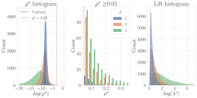
Figure 4: Left: Histogram of log max reachability values for $\beta=[1,2,4]$. Black dotted line denotes $\rho^{\star}$ for uniformly random recommender. Center: Histogram of $\rho^{\star}>0.05$ (red dotted line). Right: Histogram of log-lifts. Reachability evaluated on ML-1M for $K=5$ Random Future action space and a LibFM model.

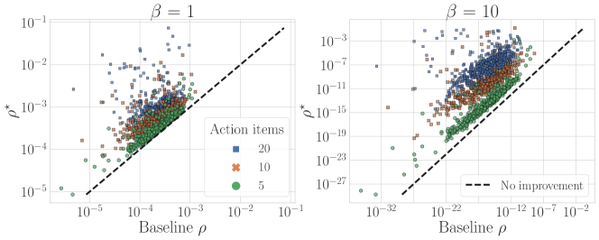
Figure 5: Log scale scatterplot of $\rho^{\star}$ values against baseline $\rho$ for $K\in[5,10,20]$. Colors indicate action space size $K$. We compare low (left) and high (right) stochasticity. Reachability evaluated on ML-1M for Random Future action space and a LibFM model.

5.2 Impact of Recommender Pipeline

We begin by examining the role of recommender pipeline components: stochasticity of item selection, user action models, and choice of preference model. All presented experiments in this section use the ML-1M dataset.

These experiments show that more stochastic recommendations correspond to higher average max reachability values, whereas more deterministic recommenders have a more disparate impact, with a small number of items achieving higher $\rho^{\star}$. We also see that the impact of the user action space differs depending on the preference model. For neighborhood based preference models, strategic manipulations to the history are most effective at maximizing reachability, whereas manipulations of the items most likely to be recommended next are ineffective.

Role of stochasticity

We investigate the role of the $\beta$ parameter in the item selection policy. Figure 4 illustrates the relationship between the stochasticity of the selection policy and max reachability. There are significantly more target items with better than random reachability for low values of $\beta$. However, higher values of $\beta$ yield more items with high reachability potential ($>5\%$ likelihood of recommendation). These items are typically items that are top-1 or close to top-1 reachable. While lower $\beta$ values provide better reachability on average and higher $\beta$ values provide better reachability at the “top”, higher $\beta$ uniformly out-performs lower $\beta$ values in terms of the lift metric. This suggests that larger $\beta$ corresponds to more user agency, since the relative effect of strategic behavior is larger. However, note that for very large values of $\beta$, high lift values are not so much the effect of improved reachability as they are due to very low baseline recommendation probabilities.

Role of user action model

We now consider different action space sizes. In Figure 5 we plot max reachability for target items of a particular user over varying levels of selection rule stochasticity and varying action space sizes. Larger action spaces correspond to improved item reachability for all values of $\beta$. However, increases in the number of action items have a more pronounced effect for larger $\beta$ values.

While increasing the size of the action space uniformly improves reachability, the same cannot be said about the type of action space. For each user, we compute the average lift over target items as a metric for user agency in a recommender (Figure 6). For LibFM, the choice of action space does not strongly impact the average user lift, though Next K displays more variance across users than the other two. However, for Item KNN, there is a stark difference between Next K and and random action spaces.

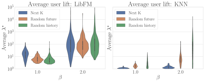
Figure 6: The distribution of average lifts (a notion of agency) over users. Colors indicate different user action spaces for LibFM (left) and KNN (right) on ML-1M.

Role of preference model

As Figure 6 illustrates, a system using LibFM provides more agency on average than one using KNN. We now consider how this relates to properties of the preference models. First, consider the fact that for LibFM, there is higher variance among user-level average lifts observed for Next K action space compared with random action spaces. This can be understood as resulting from the user-specific nature of Next K recommended items. On the other hand, random action spaces are user independent, so it is not surprising that there is less variation across users.

In a neighborhood-based model users have leverage to increase the $\rho$ reachability only for target items in the neighborhood of action items. In the case of KNN, the next items up for recommendation are in close geometrical proximity to each other. This limits the opportunity for discovery of more distant items for Next K action space. On the other hand, the action items are more uniformly over space of item ratings in random action models, thus contributing to much higher opportunities for discovery. Additionally, we see that History Edits displays higher average lift values than Future Edits. We posit that this is due to the fact that editing $K$ items from the history leads to a larger ratio of strategic to non-strategic items.

5.3 Bias in Movie, Music, and News Recommendation

We futher compare aggregated stochastic reachability against properties of user and items to investigate bias. We aggregate baseline and max reachability to compute user-level metrics of discovery and item-level metrics of availability. The audit demonstrates popularity bias for items with respect to baseline availability. This bias persists in the best case for neighborhood based recommenders and is thus unavoidable, whereas it could be mitigated for MF recommenders. User discovery aggregation reveals inconclusive results with weak correlations between the length of users’ experience and their ability to access content.

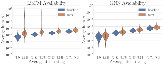
Figure 7: Comparison of baseline and best case availability of content, across four popularity categories for LibFM (left) and KNN (right) preference models. Reachability evaluated on ML-1M for Next 10 action space with $\beta=2$.

Popularity bias

In Figure 7, we plot the baseline and best case item availability (as in (3)) to investigate popularity bias. We consider popularity defined by the average rating of an item in a dataset. Another possible definition of popularity is rating frequency, but for this definition we did not observe any discernable bias. For both LibFM and KNN models, the baseline availability displays a correlation with item popularity, with Spearman’s rank-order correlations of $r_{s}=0.87$ and $r_{s}=0.95$. This suggests that as recommendations are made and consumed, more popular items will be recommended at disproportionate rates.

Furthermore, the best case availability for KNN displays a similar trend ($r_{s}=0.94$), indicating that the propagation of popularity bias can occur independent of user behavior. This does not hold for LibFM, where the best case availability is less clearly correlated with popularity ($r_{s}=0.57$). The lack of correlation for best case availability holds in the additional settings of music artist and news recommendation with the LibFM model (Figure 8). Our audit does not reveal an unavoidable systemic bias for LibFM recommender, meaning that any biases observed in deployment are due in part to user behaviour. In contrast, we see a systematic bias for the KNN recommender, meaning that regardless of user actions, the popularity bias will propagate.

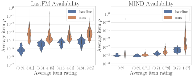
Figure 8: Comparison of baseline and best case availability of content for four popularity categories for LastFM (left) and MIND (right) with Next 10 actions, LibFM model, and $\beta=2$.

Experience bias

To consider the opportunities for discovery provided to users, we perform user level aggregations of max reachability values as in (3). We investigate experience bias by considering how the discovery metric changes as a function of the number of different items a user has consumed so far, i.e. their experience. Figure 9 illustrates that experience is weakly correlated with baseline discovery for movie recommendation ($r_{s}=0.48$), but not so much for news recommendation ($r_{s}=0.05$). The best case discovery is much higher, meaning that users have the opportunity to discover many of their target items. However, the weak correlation with experience remains for best case discovery of movies ($r_{s}=0.53$).

6 Discussion

In this paper, we generalize reachability as first defined by Dean et al. (2020) to incorporate stochastic recommendation policies. We show that for linear preference models and soft-max item selection rules, max reachability can be computed via a convex program for a range of user action models. Due to this computational efficiency, reachability analysis can be used to audit recommendation algorithms. Our experiments illustrate the impact of system design choices and historical data on the availability of content and users’ opportunities for discovery, highlighting instances in which popularity bias is inevitable regardless of user behavior.

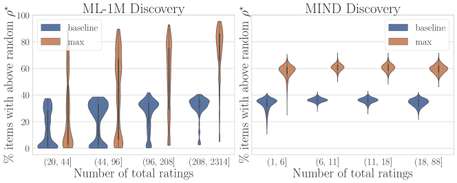
Figure 9: Comparison of baseline and best case fraction of items with better than random $\rho^{\star}$, grouped across four levels of user history length. Reachability evaluated on ML-1M (left) and MIND (right) for Next 10 action space, $\beta=2$, and LibFM model.

The reachability metric provides an upper bound for discovery and availability within a recommendation system. While it has the benefit of making minimal assumptions about user behavior, the drawback is that it allows for perfectly strategic behaviors that would require users to have full knowledge of the internal structure of the model. The results of a reachability audit may not be reflective of probable user experience, and thus reachability acts as a necessary but not sufficient condition. Nonetheless, reachability audit can lead to actionable insights by identifying inherent limits in system design. They allow system designers to assess potential biases before releasing algorithmic updates into production. Moreover, as reachability depends on the choice of action space, such system-level insights might motivate user interface design: for example, a sidebar encouraging users to re-rate $K$ items from their history.

We point to a few directions of interest for future work. Our result on the lack of trade-off between accuracy and reachability is encouraging. Minimum one-step reachability conditions could be efficiently incorporated into learning algorithms for preference models. It would also be interesting to extend reachability analysis to multiple interactions and longer time horizons.

Lastly, we highlight that the reachability lens presents a contrasting view to the popular line of work on robustness in machine learning. When human behaviors are the subject of classification and prediction, building “robustness” into a system may be at odds with ensuring agency. Because the goal of recommendation is personalization more than generalization, it would be appropriate to consider robust access over robust accuracy. This calls for questioning the current normative stance and critically examining system desiderata in light of usage context.

Appendix A Further Examples

Example 3 (Biased MF-SGD).

Biased matrix factorization models Koren and Bell [2015] compute scores as rating predictions with

$$s_{ui}=\mathbf{p}_{u}^{\top}\mathbf{q}_{i}+f_{u}+g_{i}+\mu$$

$P\in\mathbb{R}^{n\times d}$ and $Q\in\mathbb{R}^{m\times d}$ are respectively user and item factors for some latent dimension $d$, $\mathbf{f}\in\mathbb{R}^{n}$ and $\mathbf{g}\in\mathbb{R}^{m}$ are respectively user and item biases, and $\mu\in\mathbb{R}$ is a global bias.

The parameters are learned via the regularized optimization

$$\min_{P,Q,\mathbf{f},\mathbf{g},\mu}\frac{1}{2}\sum_{u}\sum_{i\in\Omega_{u}}\|\mathbf{p}_{u}^{\top}\mathbf{q}_{i}+f_{u}+g_{i}+\mu-r_{ui}\|_{2}^{2}+\frac{\lambda}{2}\|P\|_{F}^{2}+\frac{\lambda}{2}\|Q\|_{F}^{2}\>.$$

Under a stochastic gradient descent minimization scheme Koren [2008] with step size $\alpha$, the one-step update rule for a user factor is

$$\mathbf{p}^{+}_{u}=\mathbf{p}_{u}-\alpha\sum_{i\in\Omega_{u}^{\mathcal{A}}}(\mathbf{q}_{i}\mathbf{q}_{i}^{\top}\mathbf{p}_{u}+\mathbf{q}_{i}(f_{u}+g_{i}+\mu)-\mathbf{q}_{i}r_{ui})-\alpha\lambda\mathbf{p}_{u}\>.$$

User bias terms can be updated in a similar manner, but because the user bias is equal across items, it does not impact the selection of items.

Notice that this expression is affine in the mutable ratings. Therefore, we have an affine score function:

$$\phi_{u}(\mathbf{a})=Q\mathbf{p}_{u}^{+}=Q\left((1-\alpha\lambda)\mathbf{p}_{u}-\alpha Q_{\mathcal{A}}^{\top}(Q_{\mathcal{A}}\mathbf{p}_{u}+\mathbf{g}_{\cal A}+(\mu+f_{u})\mathbf{1})+\alpha Q_{\mathcal{A}}^{\top}\mathbf{a}\right)$$

where we define $Q_{\mathcal{A}}=Q_{\Omega_{u}^{\mathcal{A}}}\in\mathbb{R}^{|\Omega_{u}^{\mathcal{A}}|\times d}$ and $\mathbf{g}_{\mathcal{A}}=\mathbf{g}_{\Omega_{u}^{\mathcal{A}}}\in\mathbb{R}^{|\Omega_{u}^{\mathcal{A}}|}$. Therefore,

$$B_{u}=\alpha QQ_{\mathcal{A}}^{\top},\quad\mathbf{c}_{u}=Q\left((1+\lambda)\mathbf{p}_{u}-\alpha Q_{\mathcal{A}}^{\top}(Q_{\mathcal{A}}\mathbf{p}_{u}+\mathbf{g}_{\cal A}+(\mu+f_{u})\mathbf{1})\right)\>.$$

Example 4 (Biased MF-ALS).

Rather than a stochastic gradient descent minimization scheme, we may instead update the model with an alternating least-squares strategy Zhou et al. [2008]. In this case, the update rule is

$$\mathbf{p}^{+}_{u} =\arg\min_{\mathbf{p}}\sum_{i\in\Omega_{u}^{\mathcal{A}}\cap\Omega_{u}}\|\mathbf{p}^{\top}\mathbf{q}_{i}+f_{u}+g_{i}+\mu-r_{ui}\|_{2}^{2}+\lambda\|\mathbf{p}\|_{2}^{2}$$

$$=(Q_{u}^{\top}Q_{u}+\lambda I)^{-1}(Q^{\top}\mathbf{r}_{u}+Q_{\mathcal{A}}^{\top}(\mathbf{g}_{\mathcal{A}}+(\mu+f_{u})\mathbf{1})+Q_{\mathcal{A}}^{\top}\mathbf{a})$$

where we define $Q_{u}=Q_{\Omega_{u}^{\mathcal{A}}\cap\Omega_{u}}$. Similar to in the SGD setting, this is an affine expression, and therefore we end up with the affine score parameters

$$B_{u}=Q(Q_{u}^{\top}Q_{u}+\lambda I)^{-1}Q_{\mathcal{A}}^{\top},\quad\mathbf{c}_{u}=Q(Q_{u}^{\top}Q_{u}+\lambda I)^{-1}(Q^{\top}\mathbf{r}_{u}+Q_{\mathcal{A}}^{\top}(\mathbf{g}_{\mathcal{A}}+(\mu+f_{u})\mathbf{1}))\>.$$

Example 5 (Biased Item-KNN).

Biased neighborhood models Desrosiers and Karypis [2011] compute scores as rating predictions by a weighted average, with

$$s_{ui}=\mu+f_{u}+g_{i}+\frac{\sum_{j\in\mathcal{N}_{i}}w_{ij}(r_{uj}-\mu-f_{u}-g_{i})}{\sum_{j\in\mathcal{N}_{i}}|w_{ij}|}$$

where $w_{ij}$ are weights representing similarities between items, $\mathcal{N}_{i}$ is a set of indices which are in the neighborhood of item $i$, and $\mathbf{f},\mathbf{g},\mu$ are bias terms. Regardless of the details of how these parameters are computed, the predicted scores are an affine function of observed scores:

$$\mathbf{s}_{u}=W\mathbf{r}_{u}-W(\mathbf{g}+(\mu+f_{u})\mathbf{1})+\mathbf{g}+(\mu+f_{u})\mathbf{1}$$

where we can define

$$W_{ij}=\begin{cases}\frac{w_{ij}}{\sum_{j\in\mathcal{N}_{i}}|w_{ij}|}&j\in\mathcal{N}_{i}\\ 0&\text{otherwise}\end{cases}$$

Therefore, the score updates take the form

$$\phi_{u}(\mathbf{a})=\underbrace{W(\mathbf{r}_{u}-\mathbf{g}+(\mu+f_{u})\mathbf{1})+\mathbf{g}+(\mu+f_{u})\mathbf{1})}_{\mathbf{c}_{u}}+\underbrace{WE_{\Omega_{u}^{\mathcal{A}}}}_{B_{u}}\mathbf{a}$$

where $E_{\Omega_{u}^{\mathcal{A}}}$ selects rows of $W$ corresponding to action items.

Example 6 (SLIM and EASE).

For both SLIM Ning and Karypis [2011] and EASE Steck [2019], scores are computed as

$$s_{ui}=\mathbf{w}_{i}^{\top}\mathbf{r}_{u}$$

for $\mathbf{w}_{i}$ the row vectors of a weight matrix $W$. For SLIM, the sparse weights are computed as

$$\min_{W}~{} \frac{1}{2}\|R-RW\|_{F}^{2}+\frac{\beta}{2}\|W\|_{F}^{2}+\lambda\|W\|_{1}$$

s.t. $$W\geq 0,\mathrm{diag}(W)=0$$

For EASE, the weights are computed as

$$\min_{W}~{} \frac{1}{2}\|R-RW\|_{F}^{2}+\lambda\|W\|_{F}^{2}$$

s.t. $$\mathrm{diag}(W)=0$$

In both cases, the score updates take the form

$$\phi_{u}(\mathbf{a})=\underbrace{W\mathbf{r}_{u}}_{\mathbf{c}_{u}}+\underbrace{WE_{\Omega_{u}^{\mathcal{A}}}}_{B_{u}}\mathbf{a}\>.$$

Appendix B Datasets, Model Training and Computing Infrastructure

B.1 Detailed data description

MovieLens 1 Million

ML-1M dataset was downloaded from Group Lens via the RecLab Krauth et al. [2020] interface. It contains 1 through 5 rating data of 6040 users for 3706 movies. There are a total of 1000209 ratings (4.47% rating density). The original data is accompanied by additional user attributes such as age, gender, occupation and zip code. Our experiments didn’t indicate observable biases across these attributes. In Section D we show user discovery results split by gender.

Figure 10 illustrates descriptive statistics for the ML-1M dataset.

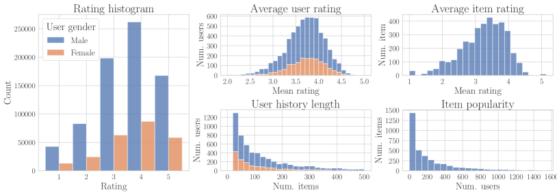
Figure 10: Descriptive statistics for the MovieLens 1M dataset split by user gender (28.3% female). The mean ratings of both users and items are roughly normally distributed while user’s history length and item popularity display power law distributions.

LastFM 360K

The LastFM 360K dataset preprocessed by Shakespeare et al. [2020] was loaded via the RecLab interface. It contains data on the number of times users have listened to various artists. We select a random subset of 10% users and a random subset of 10% items yielding 13698 users, 20109 items and 178388 ratings (0.056% rating density). The item ratings are not explicitly expressed by users as in the MovieLens case. For a user $u$ and an artist $i$ we define implicit ratings $r_{ui}=\log(\#\mathrm{listens}(u,i)+1)$. This data is accompanied by artist gender, an item attribute.

Figure 11 illustrates descriptive statistics for the LastFM dataset.

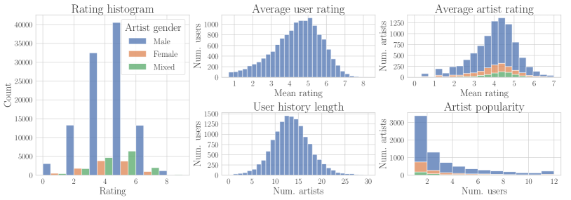
Figure 11: Descriptive statistics for the LastFM dataset split by artist gender (over 54% of artists have unknown gender, 36% are male, 6.5% are female and 3.5% are mixed gender). Unlike ML 1M, for the LastFM dataset the user history lengths are normally distributed around a mean of around 12 artists.

MIcrosoft News Dataset (MIND)

MIND is a recently published impression dataset collected from logs of the Microsoft News website . We downloaded the MIND-small dataset, which contains behaviour log data for 50000 randomly sampled users. There are 42416 unique news articles, spanning 17 categories and 247 subcategories. We aggregate user interactions at the subcategory level and consider the problem of news subcategory recommendation. The implicit rating of a user $u$ for subcategory $i$ is defined as: $r_{ui}=\log(\#\mathrm{clicks}(u,i)+1)$. The resulting aggregated dataset contains 670773 ratings (5.54% rating density).

Figure 12 illustrates descriptive statistics for the MIND dataset.

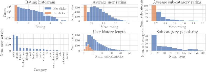
Figure 12: Descriptive statistics for the MIND dataset: The orange bars correspond to either user or items that have been displayed but have not clicked/ have not been clicked on. Unlike ML 1M and LastFM, the MIND ratings have strongly skewed distribution, with most user-subcategory ratings corresponding to users clicking on a small number of articles from the sub-category. There is a long tail of higher ratings that corresponds to most popular subcategories. The leftmost plot illustrates the unequal distribution of news articles across categories. The same qualitative behaviour holds for sub-categories.

B.2 Model Tuning

For each dataset and recommender model we perform grid search for progressively finer meshes over the tunable hyper-parameters of the recommender. We use recommenders implemented by the RecLab library. For each dataset and recommender we evaluate hyperparameters on a 10% split of test data. The best hyper-parameters for each setting are presented in Table 2.

LibFM

We performed hyper-parameter tuning to find suitable learning rate and regularization parameter for each dataset. Following Dacrema et al. [2021] we consider $\texttt{lr}\in(0.001,0.5)$ as the range of hyper-parameters for the learning rate and $\texttt{reg}\in(10^{-5},10^{0})$ for the regularization parameter. In all experimental settings we follow the setup of Rendle et al. [2019] and use 64 latent dimensions and train with SGD for 128 iterations.

KNN

We perform hyperparameter tuning with respect to neighborhood size and shrinkage parameter. Following Dacrema et al. [2021] we consider the range $(5,1000)$ for the neighborhood size and $(0,1000)$ for the shrinkage parameter. We tune KNN only for the ML-1M dataset.

Table 2: Tuning results

	LibFM
Dataset	LR	Reg.	Test RMSE	Run time (s)
ML 1M	0.0112	0.0681	0.716	2.76 $\pm$ 0.32
LastFM	0.0478	0.2278	1.122	0.78 $\pm$ 0.13
MIND	0.09	0.0373	0.318	3.23 $\pm$ 0.37
	KNN
Dataset	Neigh. size	Shrinkage	Test RMSE	Run time (s)
ML 1M	100	22.22	0.756	0.34 $\pm$ 0.07

B.3 Experimental Infrastructure and Computational Complexity

All experiments were performed on a 64 bit desktop machine equipped with 20 CPUs (Intel(R) Core(TM) i9-7900X CPU @ 3.30GHz) and a 62 GiB RAM. Average run times for training an instance of each recommender can be found in Table 2.

Appendix C Computing Reachability

C.1 Conic Program Implementation

The optimization problem in (4) is convex, and we solve it as a conic optimization problem using the MOSEK Python API under an academic license ApS [2019]. We reformulate (4) as an optimization over the exponential cone:

$$\begin{split}\min_{\begin{subarray}{c}t,\mathbf{a},\mathbf{u}\end{subarray}}~{}~{}&t-\beta(\mathbf{b}_{ui}^{\top}\mathbf{a}+c_{ui})\\ \text{s.t.}~{}~{}&\mathbf{a}\in\mathcal{A}_{u},\quad\sum_{j\in\Omega_{u}^{t}}u_{j}\leq 1,\\ &\left(u_{j},1,\beta(\mathbf{b}_{uj}^{\top}\mathbf{a}+c_{uj})-t\right)\in\mathcal{K}_{exp}~{}~{}\forall~{}~{}j\in\Omega_{u}^{t}\end{split}$$ (5)

The parameters $B_{u}$ and $\mathbf{c}_{u}$ are computed for each user based on the recommender model as described in Section A. For the LibFM model, we consider user updates with $\alpha=0.1$ and $\lambda=0$. Average run times for computing reachability of a user-item pair in various settings can be found in Table 3.

C.2 Experimental Setup for Computing Reachability

ML 1M

We compute max stochastic reachability for the LibFM and KNN preference model. We consider three types of user action spaces: History Edits, Future Edits, and Next K in which users can strategically modify the ratings associated to $K$ randomly chosen items from their history, $K$ randomly chosen items from that they have not yet seen, or the top-$K$ unseen items according to the baseline scores of the preference model. For each of the action spaces we consider $K\in\{5,10,20\}$.

We perform reachability experiments on a random 3% subset of users (176). For each choice of preference model, action space type and action space size we sample for each user 500 random items that have not been previously rated and are not action items. For each user-item pair we compute reachability for a range of stochasticity parameters $\beta\in\{1,2,4,10\}$. Note that across all experimental settings we compute reachability for the same subset of users, but different subsets of randomly selected target items.

We use the ML 1M dataset to primarily gain insights in the role that preference models, item selection stochasticity and strategic action spaces play in determining the maximum achievable degree of stochastic reachability in a recommender system.

LastFM

We run reachability experiment for LibFM recommender with Next K = 10 action model and stochasticity parameter $\beta=2$. We compute $\rho^{\star}$ values for 100 randomly sampled users and 500 randomly sampled items from the set of non-action items (target items can include previously seen items). Unlike the ML 1M dataset, the set of target items is shared among all users.

MIND

We run reachability experiments for LibFM recommender with Next K = 10 action model and stochasticity parameter $\beta=2$. We compute reachability for all items and users.

Reachability Run Times

In Table 3 we present the average clock time for computing reachability for a user-item pair in the settings described above. Due to internal representation of action spaces as matrices the runtime dependence on the dimension of the action space is fairly modest. We do not observe significant run time differences between different types of action spaces. We further add multiprocessing functionality to parallelize reachability computations over multiple target items.

Table 3: Reachability run times (in seconds).

Num. actions	ML 1M (LibFM)	ML 1M (KNN)	LastFM	MIND
K = 5	0.82 $\pm$ 0.04	9.8 $\pm$ 3.4	-	-
K = 10	0.87 $\pm$ 0.04	10.2 $\pm$ 6.1	4.91 $\pm$ 0.32	0.44 $\pm$ 0.01
K= 20	0.91 $\pm$ 0.05	11.4 $\pm$ 6.8	-	-

Appendix D Detailed Experimental Results

D.1 Impact of recommender design

We present further insights in the experimental settings studied in Section 5.2. For ML-1M, we replicate the log scale scatterplots of $\rho^{\star}$ against baseline $\rho$ for all the action spaces (Next K, Random Future, Random History), the full range of $\beta\in\{1,2,4,10\}$ and the two preference models: LibFM (Figure 13) and KNN (Figure 14). We observe that for both KNN and LibFM, random history edits can lead to higher $\rho^{\star}$ values. We posit that this increased agency is partly due to the fact that when editing $K$ items from the history a user edits a larger fraction of total ratings compared to editing $K$ future items.

The most striking feature of KNN reachability results is the strong correlation between baseline $\rho$ and $\rho^{\star}$. The correlations between baseline and max probability of recommendation is less strong in the case of LibFM. These insights are corroborated by Figure 15 which compares the average LibFM and KNN user lifts for different choices of action space, action size K, stochasticity parameter $\beta$.

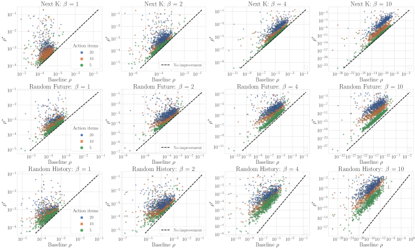
Figure 13: Log scale scatterplots of $\rho^{\star}$ against baseline $\rho$ evaluated for the LibFM preference model.

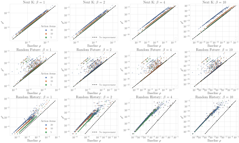
Figure 14: Log scale scatterplots of $\rho^{\star}$ against baseline $\rho$ evaluated for the KNN preference model.

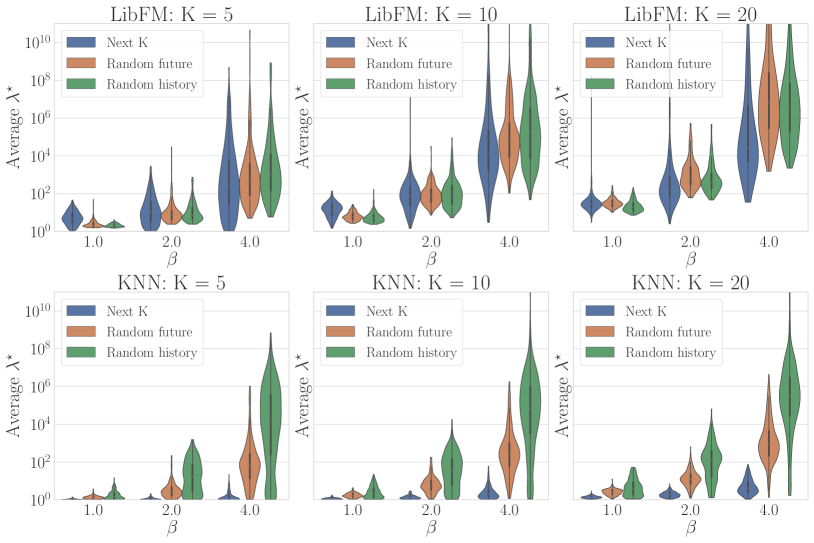
Figure 15: Side by side comparison of average user lifts for LibFM (top row)and KNN(bottom row).

D.2 Bias in movie, music, and news recommendation

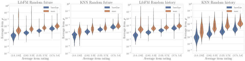
Figure 16: Side by side comparison of baseline and best-case availability of content, across four popularity categories. From left to right: LibFM preference model with Random Future, KNN preference model with Random Future, LibFM preference model with Random History, KNN preference model with Random History. Reachability evaluated on ML-1M for with $K=10$ and $\beta=2$.

We present further results on the settings studied in Section 5.3. We replicate the popularity bias results on ML-1M for different action spaces and plot the results in Figure 16. We see that the availability bias for KNN is dependent on the action space, with Random History displaying no or little correlation between popularity and max availability. This is not surprising given the results in Figure 6.

To systematically study the popularity bias, we compute the Spearman rank-order correlation coefficient to measure the presence of a monotonic relationship between popularity (as measured by average rating) and availability (either in the baseline or max case). We also compute the correlation between the popularity and the prevalence in the dataset, as measured by number of ratings.

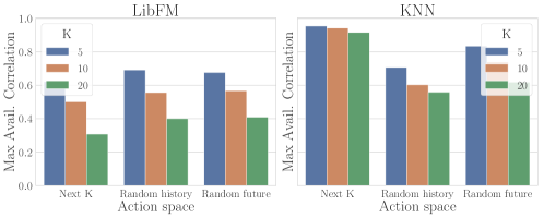
Figure 17: Comparison of Spearman’s correlation between item popularity and max availability for different action spaces and models. Reachability evaluated on ML-1M with $\beta=2$.

The impact of user action spaces is displayed in Figure 17, which plots the correlation between popularity and max availability for different action spaces. For comparison, the correlation between popularity and baseline availability is just over 0.8 for all of these settings, while the correlation with dataset prevalence is 0.346. Table 4 shows these correlation values across datasets for a fixed action model. In all cases with the LibFM model, the pattern that popularity is less correlated with max availability than baseline availability holds; however, the correlation with dataset prevalence varies.

To investigate experience bias, we similarly compute the Spearman rank-order correlation coefficient to measure the presence of a monotonic relationship between user experience (as measured by number of items rated) and discovery (either in the baseline or max case). We observe correlation values of varying sign across datasets and models, and none are particularly strong (Table 5).

Table 4: Spearman’s correlation with popularity for Next K with $K=10$ and $\beta=2$.

		corr. with	corr. with	corr. with
dataset	model	dataset prevalence	baseline availability	max availability
ml-1m	libfm	0.346280	0.827492	0.501316
ml-1m	knn	0.346280	0.949581	0.942986
mind	libfm	0.863992	0.825251	0.435212
lastfm	libfm	0.133318	0.671101	0.145949

Table 5: Spearman’s correlation with experience for Next K with $K=10$ and $\beta=2$.

		corr. with	corr. with
dataset	model	baseline discovery	max discovery
ml-1m	libfm	0.475777	0.530359
ml-1m	knn	0.206556	-0.031929
mind	libfm	0.050961	0.112558
lastfm	libfm	-0.084130	-0.089226

Finally, we investigate gender bias. We compare discovery across user gender for ML-1M and availability across artist gender for LastFM (Figure 18). We do not observe any trends in either baseline or max values.

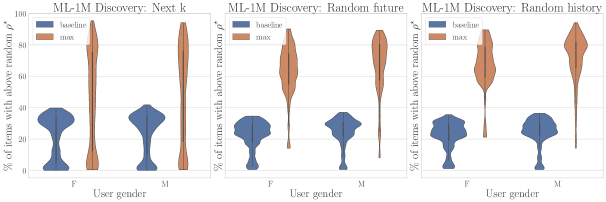
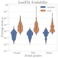
Figure 18: Side by side comparison of baseline and maximum discovery across user gender (left 3 panels) and availability across artist gender (rightmost panel). Reachability evaluated on ML-1M and LastFM with LibFM model, $K=10$, different action spaces, and $\beta=2$.

References

- Abdollahpouri et al. [2019] Himan Abdollahpouri, Masoud Mansoury, Robin Burke, and Bamshad Mobasher. The impact of popularity bias on fairness and calibration in recommendation. arXiv preprint arXiv:1910.05755, 2019.
- ApS [2019] MOSEK ApS. MOSEK Optimizer API for Python Release 9.0.88, 2019. URL https://docs.mosek.com/9.0/pythonapi.pdf.
- Castells et al. [2011] Pablo Castells, Saúl Vargas, and Jun Wang. Novelty and diversity metrics for recommender systems: choice, discovery and relevance. 2011.
- Celma [2010] Oscar Celma. Music recommendation. In Music recommendation and discovery, pages 43–85. Springer, 2010.
- Cesa-Bianchi et al. [2017] Nicolò Cesa-Bianchi, Claudio Gentile, Gábor Lugosi, and Gergely Neu. Boltzmann exploration done right. arXiv preprint arXiv:1705.10257, 2017.
- Chaney et al. [2018] Allison JB Chaney, Brandon M Stewart, and Barbara E Engelhardt. How algorithmic confounding in recommendation systems increases homogeneity and decreases utility. In Proceedings of the 12th ACM Conference on Recommender Systems, pages 224–232, 2018.
- Chen et al. [2020] Jiawei Chen, Hande Dong, Xiang Wang, Fuli Feng, Meng Wang, and Xiangnan He. Bias and debias in recommender system: A survey and future directions. arXiv preprint arXiv:2010.03240, 2020.
- Chen et al. [2019] Minmin Chen, Alex Beutel, Paul Covington, Sagar Jain, Francois Belletti, and Ed H Chi. Top-k off-policy correction for a reinforce recommender system. In Proceedings of the Twelfth ACM International Conference on Web Search and Data Mining, pages 456–464, 2019.
- Christoffel et al. [2015] Fabian Christoffel, Bibek Paudel, Chris Newell, and Abraham Bernstein. Blockbusters and wallflowers: Accurate, diverse, and scalable recommendations with random walks. In Proceedings of the 9th ACM Conference on Recommender Systems, pages 163–170, 2015.
- Dacrema et al. [2021] Maurizio Ferrari Dacrema, Simone Boglio, Paolo Cremonesi, and Dietmar Jannach. A troubling analysis of reproducibility and progress in recommender systems research. ACM Transactions on Information Systems (TOIS), 39(2):1–49, 2021.
- Dandekar et al. [2013] Pranav Dandekar, Ashish Goel, and David Lee. Biased assimilation, homophily, and the dynamics of polarization. In Proceedings of the National Academy of Sciences, pages 5791–5796, 2013.
- Dean et al. [2020] Sarah Dean, Sarah Rich, and Benjamin Recht. Recommendations and user agency: the reachability of collaboratively-filtered information. In Proceedings of the 2020 Conference on Fairness, Accountability, and Transparency, pages 436–445, 2020.
- Desrosiers and Karypis [2011] Christian Desrosiers and George Karypis. A comprehensive survey of neighborhood-based recommendation methods. Recommender systems handbook, pages 107–144, 2011.
- Ekstrand et al. [2018a] Michael D Ekstrand, Mucun Tian, Ion Madrazo Azpiazu, Jennifer D Ekstrand, Oghenemaro Anuyah, David McNeill, and Maria Soledad Pera. All the cool kids, how do they fit in?: Popularity and demographic biases in recommender evaluation and effectiveness. In Conference on Fairness, Accountability and Transparency, pages 172–186. PMLR, 2018a.
- Ekstrand et al. [2018b] Michael D Ekstrand, Mucun Tian, Mohammed R Imran Kazi, Hoda Mehrpouyan, and Daniel Kluver. Exploring author gender in book rating and recommendation. In Proceedings of the 12th ACM conference on recommender systems, pages 242–250, 2018b.
- Faddoul et al. [2020] Marc Faddoul, Guillaume Chaslot, and Hany Farid. A longitudinal analysis of youtube’s promotion of conspiracy videos. arXiv preprint arXiv:2003.03318, 2020.
- Flaxman et al. [2016] Seth Flaxman, Sharad Goel, and Justin M Rao. Filter bubbles, echo chambers, and online news consumption. Public opinion quarterly, 80(S1):298–320, 2016.
- Harper and Konstan [2015] F Maxwell Harper and Joseph A Konstan. The movielens datasets: History and context. Acm transactions on interactive intelligent systems (tiis), 5(4):1–19, 2015.
- Harper et al. [2015] F Maxwell Harper, Funing Xu, Harmanpreet Kaur, Kyle Condiff, Shuo Chang, and Loren Terveen. Putting users in control of their recommendations. In Proceedings of the 9th ACM Conference on Recommender Systems, pages 3–10, 2015.
- Herlocker et al. [2004] Jonathan Herlocker, Joseph Konstan, Loren Terveen, and John Riedl. Evaluating collaborative filtering recommender systems. ACM transactions on information systems, 22(1):5–53, 2004.
- Ie et al. [2019] Eugene Ie, Vihan Jain, Jing Wang, Sanmit Narvekar, Ritesh Agarwal, Rui Wu, Heng-Tze Cheng, Tushar Chandra, and Craig Boutilier. Slateq: A tractable decomposition for reinforcement learning with recommendation sets. 2019.
- Jannach et al. [2015] Dietmar Jannach, Lukas Lerche, Iman Kamehkhosh, and Michael Jugovac. What recommenders recommend: an analysis of recommendation biases and possible countermeasures. User Modeling and User-Adapted Interaction, 25(5):427–491, 2015.
- Karimi et al. [2020] Amir-Hossein Karimi, Gilles Barthe, Bernhard Schölkopf, and Isabel Valera. A survey of algorithmic recourse: definitions, formulations, solutions, and prospects. arXiv preprint arXiv:2010.04050, 2020.
- Kawale et al. [2015] Jaya Kawale, Hung H Bui, Branislav Kveton, Long Tran-Thanh, and Sanjay Chawla. Efficient thompson sampling for online matrix-factorization recommendation. In Advances in neural information processing systems, pages 1297–1305, 2015.
- Koren [2008] Yehuda Koren. Factorization meets the neighborhood: a multifaceted collaborative filtering model. In Proceedings of the 14th ACM SIGKDD international conference on Knowledge discovery and data mining, pages 426–434, 2008.
- Koren and Bell [2015] Yehuda Koren and Robert Bell. Advances in collaborative filtering. Recommender systems handbook, pages 77–118, 2015.
- Krauth et al. [2020] Karl Krauth, Sarah Dean, Alex Zhao, Wenshuo Guo, Mihaela Curmei, Benjamin Recht, and Michael I Jordan. Do offline metrics predict online performance in recommender systems? arXiv preprint arXiv:2011.07931, 2020.
- Lukoff et al. [2021] Kai Lukoff, Ulrik Lyngs, Himanshu Zade, J Vera Liao, James Choi, Kaiyue Fan, Sean A Munson, and Alexis Hiniker. How the design of youtube influences user sense of agency. arXiv preprint arXiv:2101.11778, 2021.
- Mary et al. [2015] Jérémie Mary, Romaric Gaudel, and Philippe Preux. Bandits and recommender systems. In International Workshop on Machine Learning, Optimization and Big Data, pages 325–336. Springer, 2015.
- Nguyen et al. [2014] Tien T Nguyen, Pik-Mai Hui, F Maxwell Harper, Loren Terveen, and Joseph A Konstan. Exploring the filter bubble: the effect of using recommender systems on content diversity. In Proceedings of the 23rd international conference on World wide web, pages 677–686, 2014.
- Ning and Karypis [2011] Xia Ning and George Karypis. Slim: Sparse linear methods for top-n recommender systems. In 2011 IEEE 11th International Conference on Data Mining, pages 497–506. IEEE, 2011.
- Rendle [2012] Steffen Rendle. Factorization machines with libFM. ACM Trans. Intell. Syst. Technol., 3(3):57:1–57:22, May 2012. ISSN 2157-6904.
- Rendle et al. [2019] Steffen Rendle, Li Zhang, and Yehuda Koren. On the difficulty of evaluating baselines: A study on recommender systems. arXiv preprint arXiv:1905.01395, 2019.
- Ribeiro et al. [2020] Manoel Horta Ribeiro, Raphael Ottoni, Robert West, Virgílio AF Almeida, and Wagner Meira Jr. Auditing radicalization pathways on youtube. In Proceedings of the 2020 conference on fairness, accountability, and transparency, pages 131–141, 2020.
- Schnabel et al. [2016] Tobias Schnabel, Adith Swaminathan, Ashudeep Singh, Navin Chandak, and Thorsten Joachims. Recommendations as treatments: Debiasing learning and evaluation. In international conference on machine learning, pages 1670–1679. PMLR, 2016.
- Shakespeare et al. [2020] Dougal Shakespeare, Lorenzo Porcaro, Emilia Gómez, and Carlos Castillo. Exploring artist gender bias in music recommendation. arXiv preprint arXiv:2009.01715, 2020.
- Singh and Joachims [2018] Ashudeep Singh and Thorsten Joachims. Fairness of exposure in rankings. In Proceedings of the 24th ACM SIGKDD International Conference on Knowledge Discovery & Data Mining, pages 2219–2228, 2018.
- Steck [2018] Harald Steck. Calibrated recommendations. In Proceedings of the 12th ACM conference on recommender systems, pages 154–162, 2018.
- Steck [2019] Harald Steck. Embarrassingly shallow autoencoders for sparse data. In The World Wide Web Conference, pages 3251–3257, 2019.
- Ustun et al. [2019] Berk Ustun, Alexander Spangher, and Yang Liu. Actionable recourse in linear classification. In Proceedings of the Conference on Fairness, Accountability, and Transparency, pages 10–19, 2019.
- Wei et al. [2017] Zeng Wei, Jun Xu, Yanyan Lan, Jiafeng Guo, and Xueqi Cheng. Reinforcement learning to rank with markov decision process. In Proceedings of the 40th International ACM SIGIR Conference on Research and Development in Information Retrieval, pages 945–948, 2017.
- Wu et al. [2020] Fangzhao Wu, Ying Qiao, Jiun-Hung Chen, Chuhan Wu, Tao Qi, Jianxun Lian, Danyang Liu, Xing Xie, Jianfeng Gao, Winnie Wu, et al. Mind: A large-scale dataset for news recommendation. In Proceedings of the 58th Annual Meeting of the Association for Computational Linguistics, pages 3597–3606, 2020.
- Yang et al. [2018] Longqi Yang, Yin Cui, Yuan Xuan, Chenyang Wang, Serge Belongie, and Deborah Estrin. Unbiased offline recommender evaluation for missing-not-at-random implicit feedback. In Proceedings of the 12th ACM Conference on Recommender Systems, pages 279–287, 2018.
- Yao et al. [2021] Sirui Yao, Yoni Halpern, Nithum Thain, Xuezhi Wang, Kang Lee, Flavien Prost, Ed H Chi, Jilin Chen, and Alex Beutel. Measuring recommender system effects with simulated users. arXiv preprint arXiv:2101.04526, 2021.
- Zhou et al. [2008] Yunhong Zhou, Dennis Wilkinson, Robert Schreiber, and Rong Pan. Large-scale parallel collaborative filtering for the netflix prize. In International conference on algorithmic applications in management, pages 337–348. Springer, 2008.