Abstract

The double descent curve is one of the most intriguing properties of deep neural networks. It contrasts the classical bias-variance curve with the behavior of modern neural networks, occurring where the number of samples nears the number of parameters. In this work, we explore the connection between the double descent phenomena and the number of samples in the deep neural network setting. In particular, we propose a construction which augments the existing dataset by artificially increasing the number of samples. This construction empirically mitigates the double descent curve in this setting. We reproduce existing work on deep double descent, and observe a smooth descent into the overparameterized region for our construction. This occurs both with respect to the model size, and with respect to the number epochs.

1 Introduction

Underparameterization and overparameterization are at the heart of understanding modern neural networks. The traditional notion of underparameterization and overparameterization led to the classic U-shaped generalization error curve (Hastie et al., 2001; Geman et al., 1992), where generalization would worsen when the model had either too few (underparameterized) or too many parameters (overparameterized). Correspondingly, it was expected that an underparameterized model would underfit and fail to identify more complex and informative patterns, and an overparameterized model would overfit and identify non-informative patterns.

This view no longer holds for modern neural networks. It is widely accepted that neural networks are vastly overparameterized, yet generalize well. There is strong evidence that increasing the number of parameters leads to better generalization (Zagoruyko and Komodakis, 2016; Huang et al., 2017; Larsson et al., 2016), and models are often trained to achieve zero training loss (Salakhutdinov, 2017), while still improving in generalization error, whereas the traditional view would suggest overfitting.

To bridge the gap, Belkin et al. (2018) proposed the double descent curve, where the underparameterized region follows the U-shaped curve, and the overparameterized region smoothly decreases in generalization error, as the number of parameters increases further. This results in a peak in generalization error, where a fewer number of samples would counter-intuitively decrease the error. There has been extensive experimental evidence of the double descent curve in deep learning (Nakkiran et al., 2019; Yang et al., 2020), as well as in models such as random forests, and one layer neural networks (Belkin et al., 2018; Ba et al., 2020).

One recurring theme in the definition of overparameterization and underparameterization lies in the number of neural network parameters relative to the number of samples (Belkin et al., 2018; Nakkiran et al., 2019; Ba et al., 2020; Bibas et al., 2019; Muthukumar et al., 2019; Hastie et al., 2019). On a high level, a greater number of parameters than samples is generally considered overparameterization, and fewer is considered underparameterization.

However, this leads to the question “What is a sample?” In this paper, we revisit the fundamental underpinnings of overparameterization and underparameterization, and stress test when it means to be overparameterized or underparameterized, through extensive experiments of a cleverly constructed input. We artificially augment existing datasets by simply stacking every combination of inputs, and show the mitigation of the double descent curve in the deep neural network setting. We humbly hypothesize that in deep neural networks we can, perhaps, artificially increase the number of samples without increasing the information contained in the dataset, and by implicitly changing the classification pipeline mitigate the double descent curve. In particular, the narrative of our paper obeys the following:

• We propose a simple construction to artificially augment existing datasets of size $O(n)$ by stacking inputs to produce a dataset of size $O(n^{2})$.

• We demonstrate that the construction has no impact on the double descent curve in the linear regression case.

• We show experimentally that those results on double descent curve do not extend to the case of neural networks.

Concretely, we reproduce recent landmark papers, presenting the differing behavior with respect to double descent.

2 Related Works

The double descent curve was proposed recently (Belkin et al., 2018), where the authors define over/underparameterization as the proportion of parameters to samples, explained through model capacity. With more parameters in the overparameterized region, there is larger “capacity” (i.e., the model class contains more candidates), and thus may contain better, simpler models by Occam’s Razor rule. The interpolation region is suggested to exist when the model capacity is capable of fitting the data nearly perfectly by overfitting on non-informative features, resulting in higher test error.

Double descent is also observed in deep neural networks (Nakkiran et al., 2019), in addition to epoch-wise double descent. Experimentation is amplified by label noise. With the observation of unimodel variance (Neal et al., 2018), Yang et al. (2020) decomposes the risk into bias and variance, and posits that double descent arises due to the bell-shaped variance curve rising faster than the bias decreases.

There is substantial theoretical work on double descent, particularly in the least squares regression setting. Advani and Saxe (2017) analyses this linear setting and proves the existence of the interpolation region, where the number of parameters equals the number of samples in the asymptotic limit. Another work Hastie et al. (2019) proves that regularization reduces the peak in the interpolation region. Belkin et al. (2019) requires only finite samples, where the features and target be jointly Gaussian. Other papers with similar setup include (Muthukumar et al., 2019; Bibas et al., 2019; Mitra, 2019; Mei and Montanari, 2019; Ba et al., 2020; Nakkiran, 2019; Bartlett et al., 2019; Chen et al., 2020).

3 Methods

We introduce the concatenated inputs construction. This way the size of a dataset can be artificially, but non-trivially, increased. This construction can be applied both to the regression setting and the classification setting. In linear regression, for given input pairs, $(x_{1},y_{1})$, $(x_{2},y_{2})$, an augmented dataset can be constructed:

$$\Big{\{}\left([x_{1},x_{1}],\tfrac{y_{1}+y_{1}}{2}\right),\left([x_{1},x_{2}],\tfrac{y_{1}+y_{2}}{2}\right),$$

$$\left([x_{2},x_{1}],\tfrac{y_{2}+y_{1}}{2}\right),\left([x_{2},x_{2}],\tfrac{y_{2}+y_{2}}{2}\right)\Big{\}},\vspace{-0.1cm}$$

where $[\alpha,\beta]$ represents concatenation of the input $\alpha,\beta$. In the setting of classification, the process is identical, where the targets are produced by element-wise addition and then averaged to sum to 1. The averaging is not strictly necessary even in the deep neural network classification case, where the binary cross entropy loss can be used instead of cross entropy. For test data, we concatenate the same input with itself, and the target is the original target. This way a dataset of size $O(n)$ is artificially augmented to size $O(n^{2})$.

Our reasons for the concatenated inputs construction are as follows: $i)$ there is limited injection of information or semantic meaning; $ii)$ the number of samples is significantly increased. For the purposes of understanding underparameterization, overparameterization and double descent, such a construction tries to isolate the definition of a sample.

4 Results

In this section, we reproduce settings from benchmark double descent papers, add the concatenated inputs construction and analyze the findings.

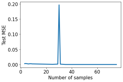
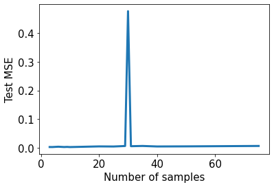
Figure 1: Left: The standard case. Right: The concatenated inputs construction. Plots of the Test MSE versus the number of samples (pre-concatenation) for min-norm ridgeless regression, where $d=30$. Following Nakkiran (2019), inputs are drawn $x\sim\mathcal{N}(0,I_{d})$, target $y=\theta x+\mathcal{N}(0,\sigma^{2})$, where $\theta$ are the parameters, $||\theta||_{2}=1$, $\sigma=0.1$. $\hat{\theta}=X^{\dagger}y$. As expected, the concatenated inputs construction does not affect the double descent curve, and the peak occurs in the exact same location.

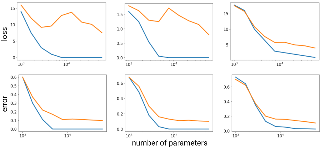
Figure 2: Top: Loss against number of parameters. Bottom: Error against number of parameters. In order from left to right: 1) Input is $32\times 32$ image, label is one-hot vector; 2) Input is $64\times 32$ image (two of the same image stacked on top of each other), label is one-hot vector; 3) Input is $64\times 32$ image (two different $32\times 32$ images stacked on top of each other), label is two-hot vector of values 0.5, 0.5. Cross Entropy loss. Orange/blue is validation/train.

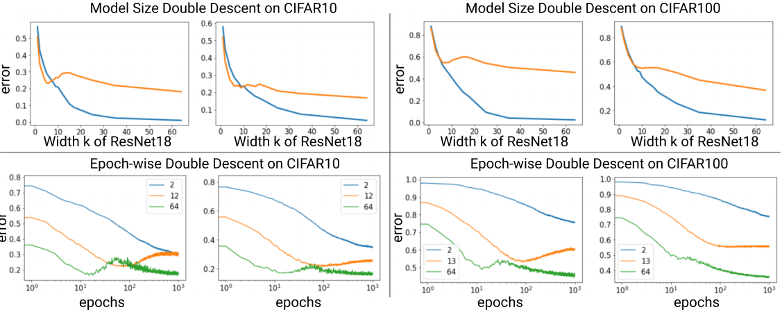
Figure 3: Top Left: Model Size Double Descent on CIFAR10. Orange line is validation error, blue line is train error. Top Right: Model Size Double Descent on CIFAR100. Orange line is validation error, blue line is train error. Bottom Left: Epoch-wise Double Descent on CIFAR10. Bottom Right: Epoch-wise Double Descent on CIFAR100. For each subplot, Left: Standard one-hot vector setup, Right: Concatenated inputs construction. Bottom plots legends’ represent the width k of the ResNet18. Models are ResNet18 architecture on CIFAR-10 and CIFAR-100 datasets.

4.1 Linear regression

The linear regression setting has been a fruitful testbed for empirical work in double descent, as well as yielding substantial theoretical understanding. The concatenated inputs construction is applied similarly here, however with different motivation. Namely, we wish to motivate that the concatenated inputs construction is not expected to add any information and is therefore not expected to impact the double descent curve.

We reproduce the linear regression setting from Nakkiran (2019), given in Figure 1. For the concatenated inputs construction, we first draw the number of samples before concatenation and construction of the augmented dataset. We observe that, by construction, the concatenated inputs construction does not affect the double descent curve, and the peak occurs in the exact same location. We also remark here that it is not surprising, and it is not complicated to understand why from a theoretical perspective.

4.2 One hidden layer feedforward neural network

We train a feedforward neural network with one hidden ReLU layer on MNIST, reproducing the setup from Belkin et al. (2018). We vary the number of parameters by changing the size of the hidden layer (see Figure 2).

We observe in the upper-right plot in Figure 2 the double descent curve is completely removed in the concatenated inputs construction relative to the other two settings. A smooth decrease in loss is observed, while there is a clear double descent in the other cases (upper-left/middle plots in Figure 2). Furthermore, when concatenating each input only by itself (upper-middle plot in Figure (2)), the double descent curve is present almost exactly.This provides evidence that the disappearance of the double descent is not due to the extra parameters, which originate from the larger sized inputs. In this setting, it appears that the behavior of under/overparameterization can be altered by artificially increasing the number of samples through concatenation.

In addition, the model trained on MNIST and one-hot vectors can be concatenated with itself, with all other parameters being zero, to produce a model with two times the number of hidden units which can be applied to the concatenated inputs construction. We consider this setting in the context of a possible explanation of the interpolation region, where the number of parameters nears that of samples. Concretely, it is possible for a neural network with double the hidden units in the concatenated inputs construction to recover the double descent curve by learning two smaller, disconnected networks, where each of the smaller networks are the ones learned in the double descent peak of the standard, one-hot case. However, in practice while the network can do so, it does not appear to, which leads to the smooth descent in Figure 2.

4.3 Deep Neural Networks

Model size double descent. We train a ResNet18 on CIFAR10 (top row in Figure 3), reproducing the setup from Nakkiran et al. (2019). We vary the number of parameters in the neural network by changing the width $k$. Immediately, we see that the double descent curve is relatively mitigated in the case of the concatenated inputs construction where we vary $k$ from $k=5$ to $20$. Here, the curve is much smoother, although not entirely smooth (see left (regular) and right (concatenated) subplots in the Top-Left cluster in Figure 3). Notably, the concatenated inputs construction retains the test error across $k$, except in the interpolation region where it achieves significantly lower test error ($>5\%$). The conclusion is identical when error is plotted against parameters, since the concatenated inputs construction typically adds a very few parameters ($<5\%$). We see this pattern repeated on CIFAR-100 (Figure 3, Top-right cluster).

Epoch-wise double descent. We use the same setting, except we train models for an additional 600 epochs, totaling 1000. In Figure 3, Bottom row, we consider the ResNet18 architecture for CIFAR10 (Left cluster of plots) and CIFAR100 (Right cluster of plots). We plot test error against epochs. In the one hot setting (let us focus on the left plot of CIFAR10 case), as expected, we observe a U shape for medium sized models and a double descent for larger models (Nakkiran et al., 2019). For concatenated inputs (Right plot of CIFAR10 case), a flat U shape and double descent is existent, but significantly mitigated. The mitigation allows a 5% improvement at the end of training for medium sized models and a 10% improvement in the middle of training for large models. We see similar results on CIFAR-100, where double descent disappears with concatenated inputs.

4.4 Bias Variance decomposition

In this section, we follow Yang et al. (2020) and decompose the loss into bias and variance. Namely, let CE denote the cross entropy loss, $T$ a random variable representing the training set, $\pi$ is the true one-hot label, $\bar{\pi}$ is the average log-probability after normalization, and $\hat{\pi}$ is the output of the neural network. Then,

$$\mathbb{E}_{T}[\texttt{CE}(\pi,\hat{\pi})]=D_{KL}(\pi||\bar{\pi})+\mathbb{E}_{T}[D_{KL}(\bar{\pi}||\hat{\pi})]$$

where the first component is the bias and the second component is the variance. On a high level, the variance can then be estimated by training separate same capacity models on different splits of the dataset, and then measuring the difference in outputs on the same test set. The bias is then computed by subtracting the empirical variance from the empirical risk. For finer details, see Yang et al. (2020)

For training, we follow Yang et al. (2020) and train a ResNet-34 (He et al., 2016) on CIFAR10, with stochastic gradient descent (learning rate $=0.1$, momentum $=0.9$). The learning rate is decayed a factor of 0.1 every 200 epochs, with a weight decay of 5e-4. The width $k$ of the network is varied suitably between 1 and 64. We also make 5 splits of 10,000 training samples for the calculation of bias/ variance.

We present results in Figure 4. The concatenated inputs construction significantly delays and smoothens the increase in variance relative to the standard case, where the unimodal variance is significantly sharper. This impacts the shape of the test error, where in this setting we see a shifted bump in test error for the concatenated inputs construction. One possible explanation is in the case of deep neural networks the concatenated inputs construction is a form of implicit regularization for small models, which controls overfitting and leads to a smoother variance curve.

5 Discussion

While the understanding of over/underparameterization and double descent is strongly tied to the number of samples, it appears that given a fixed number of unique samples it is possible to manipulate over/underparameterization by artificially boosting the number of samples by the concatenated inputs construction.

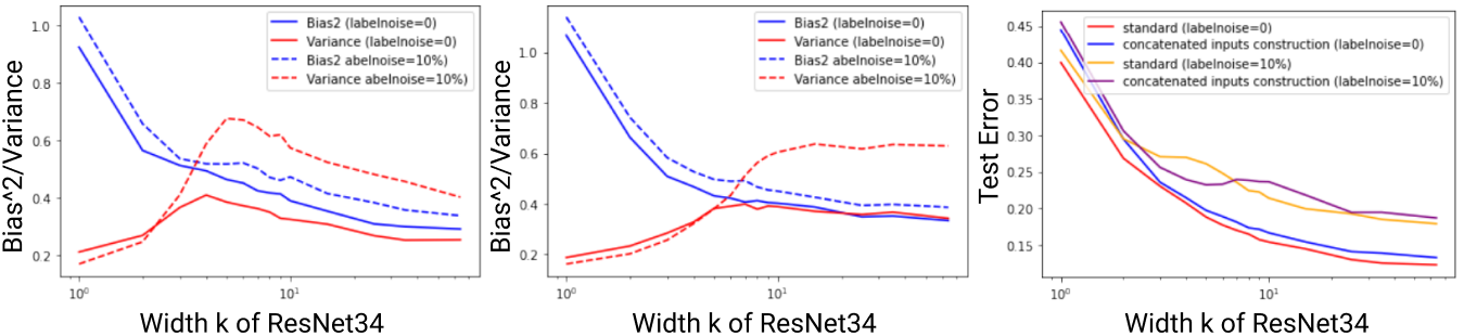
Figure 4: Left: Bias and Variance against width k of ResNet-34 in the standard case. Middle: Bias and Variance against width k of ResNet-34 in the concatenated inputs construction. Right: Test error against width k of ResNet-34 in the standard case and concatenated inputs construction.

A possible explanation in the literature for double descent is that the model is being forced to fit the training data as perfectly as possible, and at some model capacity it is possible to fit the training data perfectly by overfitting on non-existent, or weakly present, features. This results in overfitting and the double descent curve. Interestingly, the concatenated inputs construction generally mitigates double descent, even though it is possible to build models for the concatenated inputs construction from models for the standard setting. This suggests a possible route to improve the understanding of the relationship to the model capacity.

The experimental results in this work support that neural network behavior can change with respect to the number of samples, even if the majority of samples add limited information, via the concatenated inputs construction. In this view, the concatenated inputs construction creates possibly a huge dataset, e.g. $50,000^{2}$ samples for the originally $50,000$ samples CIFAR10 where $50,000^{2}$ = 2,500,000,000 is far larger than any neural network for CIFAR10. Yet, there is no noticeable underfitting. Namely, the concatenated inputs construction quickly achieves comparable performance to the standard one-hot vector deep learning setting. This suggests we may need to rethink the relationship between underfitting, the number of parameters, samples, and model capacity.

References

- (1)
- Advani and Saxe (2017) Madhu S Advani and Andrew M Saxe. 2017. High-dimensional dynamics of generalization error in neural networks. arXiv preprint arXiv:1710.03667 (2017).
- Ba et al. (2020) Jimmy Ba, Murat Erdogdu, Taiji Suzuki, Denny Wu, and Tianzong Zhang. 2020. Generalization of Two-layer Neural Networks: An Asymptotic Viewpoint. In ICLR.
- Bartlett et al. (2019) Peter L Bartlett, Philip M Long, Gabor Lugosi, and Alexander Tsigler. 2019. Benign overfitting in linear regression. arXiv preprint arXiv:1906.11300 (2019).
- Belkin et al. (2018) Mikhail Belkin, Daniel Hsu, Siyuan Ma, and Soumik Mandal. 2018. Reconciling modern machine learning practice and the bias-variance trade-off. arXiv preprint arXiv:1812.11118 (2018).
- Belkin et al. (2019) Mikhail Belkin, Daniel Hsu, and Ji Xu. 2019. Two models of double descent for weak features. arXiv preprint arXiv:1903.07571 (2019).
- Bibas et al. (2019) Koby Bibas, Yaniv Fogel, and Meir Feder. 2019. A new look at an old problem: A universal learning approach to linear regression. arXiv preprint arXiv:1905.04708 (2019).
- Chen et al. (2020) Lin Chen, Yifei Min, Mikhail Belkin, and Amin Karbasi. 2020. Multiple Descent: Design Your Own Generalization Curve. arXiv:2008.01036 [cs.LG]
- Geman et al. (1992) Stuart Geman, Elie Bienenstock, and Ren Doursat. 1992. Neural networks and the bias/variance dilemma. Neural Computation (1992).
- Hastie et al. (2019) Trevor Hastie, Andrea Montanari, Saharon Rosset, and Ryan J Tibshirani. 2019. Surprises in high dimensional ridgeless least squares interpolation. arXiv preprint arXiv:1903.08560 (2019).
- Hastie et al. (2001) Trevor Hastie, Robert Tibshirani, and Jerome Friedman. 2001. The Elements of Statistical Learning, volume 1. Springer (2001).
- He et al. (2016) Kaiming He, Xiangyu Zhang, Shaoqing Ren, and Jian Sun. 2016. Deep residual learning for image recognition. In Proceedings of the IEEE conference on computer vision and pattern recognition. 770–778.
- Huang et al. (2017) Gao Huang, Zhuang Liu, Laurens Van Der Maaten, and Kilian Q. Weinberger. 2017. Densely connected convolutional networks. In CVPR.
- Larsson et al. (2016) Gustav Larsson, Michael Maire, and Gregory Shakhnarovich. 2016. Ultra-deep neural networks without residuals. arXiv preprint arXiv:1605.07648 (2016).
- Mei and Montanari (2019) Song Mei and Andrea Montanari. 2019. The generalization error of random features regression: Precise asymptotics and double descent curve. arXiv preprint arXiv:1908.05355 (2019).
- Mitra (2019) Partha P. Mitra. 2019. Understanding overfitting peaks in generalization error: Analytical risk curves for l2 and l1 penalized interpolation. arXiv preprint arXiv:1906.03667 (2019).
- Muthukumar et al. (2019) Vidya Muthukumar, Kailas Vodrahalli, and Anant Sahai. 2019. Harmless interpolation of noisy data in regression. arXiv preprint arXiv:1903.09139 (2019).
- Nakkiran (2019) Preetum Nakkiran. 2019. More Data Can Hurt for Linear Regression: Sample-wise Double Descent. arXiv:1912.07242 [stat.ML]
- Nakkiran et al. (2019) Preetum Nakkiran, Gal Kaplun, Yamini Bansal, Tristan Yang, Boaz Barak, and Ilya Sutskever. 2019. Deep double descent: Where bigger models and more data hurt. arXiv preprint arXiv:1912.02292 (2019).
- Neal et al. (2018) Brady Neal, Sarthak Mittal, Aristide Baratin, Vinayak Tantia, Matthew Scicluna, Simon Lacoste-Julien, and Ioannis Mitliagkas. 2018. A Modern Take on the Bias-Variance Tradeoff in Neural Networks. arXiv:1810.08591 [cs.LG]
- Salakhutdinov (2017) Ruslan Salakhutdinov. 2017. Deep learning tutorial at the Simons Institute, Berkeley. https://simons.berkeley.edu/talks/ruslan-salakhutdinov-01-26-2017-1 (2017).
- Yang et al. (2020) Zitong Yang, Yaodong Yu, Chong You, Jacob Steinhardt, and Yi Ma. 2020. Rethinking Bias-Variance Trade-off for Generalization of Neural Networks. arXiv preprint arXiv:2002.11328 (2020).
- Zagoruyko and Komodakis (2016) Sergey Zagoruyko and Nikos Komodakis. 2016. Wide residual networks. arXiv preprint arXiv:1605.07146 (2016).