Flow-based sampling for multimodal distributions in lattice field theory

Abstract

Recent results have demonstrated that samplers constructed with flow-based generative models are a promising new approach for configuration generation in lattice field theory. In this paper, we present a set of methods to construct flow models for targets with multiple separated modes (i.e. theories with multiple vacua). We demonstrate the application of these methods to modeling two-dimensional real scalar field theory in its symmetry-broken phase. In this context we investigate the performance of different flow-based sampling algorithms, including a composite sampling algorithm where flow-based proposals are occasionally augmented by applying updates using traditional algorithms like HMC.

I Introduction

Quantum field theories (QFTs) are the mathematical and conceptual frameworks through which we describe particle-based theories of Nature. For example, the Standard Model of particle physics encapsulates our current best understanding of fundamental particles and their interactions in terms of a QFT. Deriving physical results from QFTs such as the Standard Model in many cases requires calculations in strong-coupling regimes of the theories, for which perturbative methods cannot be applied. Lattice quantum field theory Morningstar (2007) provides a non-perturbative approach to computing physical quantities in this regime based on numerically evaluating path integrals, rendered finite and regularized by discretizing the quantum fields onto a Euclidean spacetime lattice. This method is commonly applied to determine strong force phenomena described by Quantum Chromodynamics (QCD) within the Standard Model Lehner et al. (2019); Kronfeld et al. (2019); Cirigliano et al. (2019); Detmold et al. (2019); Bazavov et al. (2019); Joó et al. (2019), and also is used in studies of beyond–Standard-Model theories Brower et al. (2019); DeGrand (2016); Svetitsky (2018); Kribs and Neil (2016). Lattice methods are also widely applied in condensed matter physics to determine quantum and classical collective phenomena of many degrees of freedom Mathur and Sreeraj (2016).

In both particle physics and condensed matter applications it is important to extrapolate lattice field theory calculations to a large number of degrees of freedom (lattice sites) and a long correlation length, giving access to continuum/infinite-volume physics and physics near critical points. Calculations approaching these limits, however, have diverging computational cost due to the phenomenon of “critical slowing down” in typical Markov Chain Monte Carlo (MCMC) approaches to sampling the path integral in these theories Wolff (1990); Del Debbio et al. (2004); Meyer et al. (2007); Schaefer et al. (2009, 2011). Intuitively, this slowing down occurs for algorithms that draw successive samples by applying close-to-local stochastic perturbations to previous samples; when correlation lengths are large and there are many degrees of freedom, many stochastic steps are required before arriving at a new independent sample. In some cases, carefully designed algorithms have been shown to alleviate this growing computational cost Hoshen and Kopelman (1976); Wolff (1988); Swendsen and Wang (1987); Edwards and Sokal (1988); Wolff (1989); Brower and Tamayo (1989); Hasenbusch (1990); Sinclair (1992); Bietenholz et al. (1995); Evertz (2003); Prokof’ev and Svistunov (2001); Kawashima and Harada (2004); Azcoiti et al. (2009); Gattringer et al. (2015); Bernard et al. (2009); Michel et al. (2015); Nishikawa et al. (2015); Hasenbusch and Schaefer (2018); Lei and Krauth (2018), typically by applying more non-local stochastic updates, but such methods have not been found for key theories including QCD.

There are growing efforts to apply machine learning techniques to accelerate sampling for lattice field theories with the goal of enabling calculations which are currently computationally intractable Wang (2017); Huang and Wang (2017); Song et al. (2017); Levy et al. (2018); Li and Wang (2018); Wu et al. (2019); Albergo et al. (2019); Kanwar et al. (2020); Boyda et al. (2021); Pawlowski and Urban (2020); Nicoli et al. (2020a, b); Albergo et al. (2021). One such approach uses flow-based models to independently sample field configurations. In this framework, the flow model defines a variational proposal distribution that can be optimized to approximate the physical distribution of interest. The flow-based MCMC algorithm developed in Refs. Albergo et al. (2019); Kanwar et al. (2020); Boyda et al. (2021) uses proposals generated by flow models with a corrective Metropolis-Hastings accept/reject step, which grants theoretical guarantees of asymptotic exactness in the same way that more traditional sampling methods such as hybrid/Hamiltonian Monte Carlo (HMC) Duane et al. (1987) do.

For both traditional methods and flow-based MCMC these guarantees of exactness are asymptotic, and in practice a finite ensemble of samples may not be sufficient to achieve a representative sampling and unbiased results. However, as we discuss and demonstrate in this work, traditional methods and flow-based MCMC can exhibit poor sampling behavior in different ways, and can be combined to produce efficient samplers where either method would fail individually. Multimodal distributions provide a clear example where this is the case, and are the focus of this work.

In particular, finite-sample pathologies have been demonstrated for traditional methods in cases where the sampling algorithm remains trapped in one or several of many modes of a multimodal distribution, such as when “topological freezing” occurs Del Debbio et al. (2004); Schaefer et al. (2009, 2011); Hasenbusch (2018). Meanwhile, the efficiency of flow-based MCMC depends on how well the model approximates the target distribution: models that undersample particular regions of the target distribution result in inefficient samplers due to long runs of rejected proposals, requiring many proposal steps before asymptotic convergence. When used in combination, the two methods may correct each other’s respective deficiencies, with flow proposals providing rapid mixing between modes while updates with traditional methods populate regions undersampled by the flow model. However, this complementarity requires flow models that sample from all modes of the target.

In this work, we first explore and demonstrate the capacity of flow-based methods to model multimodal distributions. As a testbed, we study the particular example of two-dimensional real scalar field theory. With quadratic and quartic interactions, this theory has a $Z_{2}$ global symmetry (negation of the field) and a corresponding broken-symmetry phase for which the distribution of fields is bimodal. Adding a linear interaction breaks the symmetry explicitly, providing a model for the more general case of multiple modes with different shapes and relative weights. In either the exactly symmetric or explicitly broken case, we have a mean-field description of the mode structure and a known operation (negation) which moves fields between modes. As a test of generic approaches to modeling multimodal distributions without such a priori knowledge, we use flow model architectures which do not explicitly encode this mode structure. In this context, we find that training using stochastic gradient descent with default hyperparameters using the “reverse KL” self-training procedure employed in e.g. Refs. Albergo et al. (2019); Kanwar et al. (2020); Boyda et al. (2021); Albergo et al. (2021) often results in “mode-collapsed” models that sample only single modes of the distribution. We demonstrate how these mode-collapsed models can be used to construct multimodal mixture models, as well as several alternate training schemes that can train multimodal models without mode collapse where, in some cases, reverse KL self-training cannot.

We then investigate the performance of the resulting models when used with both flow-based MCMC as well as a composite sampling algorithm where flow-based proposals are occasionally augmented by applying updates with HMC. While the models are good approximations of the bulk of the bimodal target distribution, they typically exhibit underweighting of the “inner tails” (regions of low density between modes). For the models trained here, we find that this underweighting can be severe enough to compromise the pure flow-based MCMC approach, with rare samples from the inner tails triggering catastrophically long runs of rejections. However, we further demonstrate that augmenting the pure flow-based proposals with HMC regulates this issue to provide an efficient sampler that outperforms HMC and gives more reliable sampling than flow-based MCMC alone.

The rest of the paper is structured as follows. In Sec. II we review traditional and flow-based MCMC methods, highlighting the different sampling challenges for each with an emphasis on how these challenges arise when sampling from multimodal distributions. In Sec. III we discuss composite MCMC updates and augmented MCMC in a general framework. Sections IV and V present a general suite of methods for constructing multimodal models. Specifically, Sec. IV discusses how generative mixtures may be constructed from mode-collapsed flow models, while Sec. V discusses different ways of training flow models that circumvent the issues of the reverse KL self-training approach employed in previous works. In Sec. VI, we apply these methods to construct flow models for the example of real scalar field theory in two dimensions. In Sec. VII, we examine the performance of the resulting models when used with flow-based MCMC and the composite algorithm, including an asymptotic analysis of the problems that arise in flow-based MCMC and how the composite algorithm resolves them. In Sec. VIII, we discuss possible extensions and alternative approaches to the methods presented in this work. In Sec. IX we present our conclusions.

II Challenges in sampling multimodal distributions

In field theory, expectation values of physical observables are obtained by evaluating path integrals over configuration space. By discretizing quantum field theories on a lattice in Euclidean spacetime, one can evaluate path integrals nonperturbatively. The expectation value of an observable $\mathcal{O}$ can be expressed as:

$$\langle\mathcal{O}\rangle=\frac{1}{Z}\int{d\phi~{}\mathcal{O}(\phi)~{}e^{-S_{E}(\phi)}},\;\,\,Z=\int{\mathcal{D}\phi~{}e^{-S_{E}(\phi)}},$$ (1)

where $\int d\phi$ denotes the path integral over the space of field configurations $\phi$ and $S_{E}$ is the Euclidean action. With the field degrees of freedom discretized on a lattice, this integral is finite but very high-dimensional, and can be recast as an expectation value $\langle\mathcal{O}\rangle_{p}$ with respect to the distribution $p(\phi)=e^{-S_{E}(\phi)}/Z$, as long as $S_{E}$ is real. The path integral of Eqn. (1) can then be approximated in a systematically improvable way by computing stochastic estimators of observable expectation values

$$\langle\mathcal{O}\rangle_{p}\approx\frac{1}{N}\sum_{i=1}^{N}{\mathcal{O}(\phi_{i})}$$ (2)

over $N$ samples of field configurations $\phi_{i}\sim p$ (i.e. drawn from the distribution $p$).

In the following, we distinguish between two general approaches to sampling high-dimensional distributions relevant for lattice field theories:

1. Update-based sampling — sampling using MCMC, producing each new field configuration by stochastically perturbing the previous configuration in the Markov chain. This class of samplers includes the Metropolis-Hastings accept/reject step applied with a proposal based on local updates Metropolis et al. (1953); Hastings (1970), heat bath updates to subsets of variables Creutz (1979); Cabibbo and Marinari (1982); Kennedy and Pendleton (1985), and HMC Duane et al. (1987).

2. Flow-based sampling — using flow-based models to generate independent configurations distributed according to an approximation of the desired probability density. Asymptotically unbiased estimates of expectation values can be computed using e.g. reweighting or independence Metropolis Tierney (1994). Though the latter is an MCMC sampler, we distinguish this approach from updated-based sampling based on the independence of the proposed updates.

High-dimensional multimodal distributions present challenges to both update-based samplers and flow-based samplers for different reasons. We explore these difficulties in the following sections, and find that the distinct challenges faced in flow-based sampling for multimodal distributions suggest new approaches to mitigate these challenges.

II.1 MCMC and the Metropolis algorithm

For many high-dimensional distributions, exact sampling schemes are not known. In these cases, MCMC provides a very general approach to drawing samples with asymptotically correct statistics Brooks et al. (2011). MCMC methods implement importance sampling by constructing a Markov chain of consecutive configurations $\phi_{0},\phi_{1},\ldots,\phi_{N}$ generated by a Markov process which satisfies balance with respect to the target distribution. The balance condition guarantees that the target distribution is fixed under the stochastic updates that define the Markov process and, assuming ergodicity, results in samples distributed according to the target distribution in the limit of a large number of updates Meyn and Tweedie (2012).

Appropriate Markov processes can be conveniently constructed using the Metropolis algorithm Metropolis et al. (1953); Hastings (1970): given the current configuration $\phi_{i}$, one determines the next configuration $\phi_{i+1}$ by proposing an update $\phi^{\prime}$ with (conditional) probability $T(\phi_{i}\rightarrow\phi^{\prime})$ and then accepting or rejecting the proposal with probability

$$p_{\text{acc.}}(\phi_{i}\rightarrow\phi^{\prime})=\min\left[1,~{}\frac{T(\phi^{\prime}\rightarrow\phi_{i})}{T(\phi_{i}\rightarrow\phi^{\prime})}\frac{p(\phi^{\prime})}{p(\phi_{i})}\right].$$ (3)

If the proposal is accepted, the next configuration is $\phi_{i+1}=\phi^{\prime}$; if rejected, then the previous configuration is repeated, $\phi_{i+1}=\phi_{i}$. The resulting Markov process satisfies a stronger form of balance, known as “detailed balance”, guaranteeing the correct stationary distribution. Any method of generating proposals is acceptable as long as it is ergodic and $T(\phi_{i}\rightarrow\phi^{\prime})/T(\phi^{\prime}\rightarrow\phi_{i})$ is computable.

As familiar in the lattice field theory context, MCMC algorithms require an initial thermalization or “burn-in” period before they begin generating target-distributed samples. In addition, a Markov chain must be sufficiently long to reach the regime where expectation values evaluated over the chain converge smoothly in $1/\sqrt{N}$ to their asymptotic values, i.e. that the true sampling distributions of means over chains of length $N$ are approximately Gaussian. Away from this regime, finite-sample error estimates can severely underestimate the true sampling variance, leading to unreliable results. As discussed below, a slow approach to this smoothly converging regime can be a practical issue for either update-based or flow-based methods, especially when sampling multimodal distributions.

II.2 Sampling challenges for update-based methods

In update-based sampling methods, each Markov chain step produces a new configuration that is a perturbation of the previous configuration. To satisfy detailed balance, these steps preferentially move towards directions of higher probability density. When the target distribution is multimodal with widely separated modes, this approach encounters severe difficulties: regions between modes must be traversed by the sampler to successfully sample from all modes, but by detailed balance this can happen only rarely when updates are local perturbations. As modes become increasingly separated, the characteristic “tunneling time” for the sampler to move from one mode to another grows rapidly, sometimes referred to as “freezing”. The Markov chain generated by the sampler will not yield smoothly converging results until many such tunneling events have occurred. This effect thus rapidly increases the sample sizes required to obtain unbiased results, presenting an obstacle for traditional MCMC methods.

II.3 Flow models and reverse KL self-training

Flow-based models are variational ansatzë for probability distributions constructed using normalizing flows Rezende and Mohamed (2016); Dinh et al. (2016); Papamakarios et al. (2019). Each model is a generative parametrization (i.e. exact/direct sampler) for a “model distribution” $\tilde{p}$ and comprises a simple, tractably sampleable prior distribution $r(z)$ and an invertible function or “flow”, $f(z)$, which maps from the latent-space variables $z$ of the prior distribution to the target-space variables $\phi$ of the model distribution. Sampling proceeds simply by drawing independent samples from the prior distribution $z\sim r$ and applying the flow to obtain independent samples from the model, $f(z)=\phi\sim\tilde{p}$. Conservation of probability gives the model density in terms of the prior density as

$$\tilde{p}(\phi)=\tilde{p}(f(z))=\left\lvert\det\frac{\partial f(z)}{\partial z}\right\rvert^{-1}r(z)$$ (4)

so we can evaluate $\tilde{p}(\phi)$ if $r(z)$ is known and the Jacobian determinant is practically computable. When applying $f$ to flow “forwards” from the prior space to the target this expression can be used to compute the model density for each sample as it is generated, and when applying $f^{-1}$ to flow “backwards” it allows evaluation of the model density for any given configuration, including those generated using other samplers. Flows are often built from a sequence of simple “coupling layers” parametrized by neural networks which each partition the variables and transform one subset conditioned on the other; this guarantees invertibility and yields a simple triangular Jacobian whose determinant can be computed efficiently Dinh et al. (2016).

Given a flow model sampler for a density $\tilde{p}(\phi)$, we can obtain asymptotically correct results for observables under the target density $p(\phi)$ in several ways. One approach to statistical correction is to apply reweighting with weights

$$w(\phi)\equiv\frac{p(\phi)}{\tilde{p}(\phi)}$$ (5)

such that expectation values are computed as

$$\langle\mathcal{O}\rangle_{p}=\langle w\mathcal{O}\rangle_{\tilde{p}}\approx\frac{1}{N}\sum_{i}w(\phi_{i})~{}\mathcal{O}(\phi_{i})$$ (6)

using model samples $\phi_{i}\sim\tilde{p}$. Alternately, one may use the flow to generate proposals for the Metropolis algorithm (flow-based MCMC). Because the samples drawn from the flow are independent, the conditional proposal density simplifies as ${T(\phi_{i}\rightarrow\phi^{\prime})=\tilde{p}(\phi^{\prime})}$ and the acceptance rate is

$$p_{\text{acc.}}(\phi_{i}\rightarrow\phi^{\prime}) =\min\left(1,\frac{\tilde{p}(\phi_{i})}{\tilde{p}(\phi^{\prime})}\frac{p(\phi^{\prime})}{p(\phi_{i})}\right)$$ (7)

$$=\min\left(1,\frac{w(\phi^{\prime})}{w(\phi_{i})}\right).$$

This special case is known as “independence Metropolis” Tierney (1994). Unlike update-based methods where proposals are perturbations of previous samples, each accepted sample is a global update of the field and the only autocorrelations in the Markov chain arise from rejections. Thus, given that flow-based samplers can be constructed with sufficiently well-behaved distributions of reweighting factors, they can circumvent problems in sampling like critical slowing down Albergo et al. (2019) and topological freezing Kanwar et al. (2020).

Many previous works using flow models Albergo et al. (2019); Kanwar et al. (2020); Boyda et al. (2021); Nicoli et al. (2020b); Gabrié et al. (2021); Del Debbio et al. (2021); Albergo et al. (2021) have optimized models by minimizing a stochastic estimate of a modified reverse Kullback-Leibler (KL) divergence,

$$\begin{split}L(\tilde{p},p)&=D_{\mathrm{KL}}(\tilde{p}||p)-\log Z\\ &=\int{\mathcal{D}\phi~{}\tilde{p}(\phi)(\log\tilde{p}(\phi)-\log p(\phi)-\log Z)}\\ &=\int{\mathcal{D}\phi~{}\tilde{p}(\phi)(\log\tilde{p}(\phi)+S(\phi))}\\ &\approx\frac{1}{N}\sum_{i=1}^{N}{\log\tilde{p}(\phi_{i})+S(\phi_{i})},\quad(\phi_{i}\sim\tilde{p}).\end{split}$$ (8)

In each step of “reverse KL self-training” the loss $L$ is estimated by drawing a batch of configurations $\phi_{i}$ with accompanying densities $\tilde{p}(\phi_{i})$ from the model, computing the action of each resulting configuration to obtain $\exp[-S(\phi_{i})]\propto p(\phi_{i})$, then varying the model parameters to minimize the reverse KL divergence using standard stochastic gradient descent methods. This self-training procedure does not require pre-generation of training data with another sampling method, and because a new batch is drawn for each training step, the training dataset is effectively infinite in size. However, as discussed in the next section, self-training procedures, and especially those using the reverse KL loss, have inherent difficulties in the context of multimodal distributions.

II.4 Sampling challenges for flow-based MCMC

If the prior distribution of a flow model has support over all field space and its flow is invertible, then the model distribution also has support over all field space. Flow-based MCMC therefore provides an ergodic Markov chain step, and estimates of expectations under the target are asymptotically unbiased. However, while nonzero, the support may be arbitrarily small in some region so that the model yields configurations from that part of field space only rarely. This admits a pathology where, when these regions are also severely underweighted in the model relative to the target, estimates computed using the flow-based sampler will converge extremely slowly: the sampler must eventually propose some configuration $\phi$ in this region for which $p(\phi)/\tilde{p}(\phi)\gg 1$, which is always accepted because this factor saturates the acceptance probability Eqn. (3); subsequent proposals to move from $\phi\rightarrow\phi^{\prime}$ are almost certainly rejected because this factor appears in inverse in the acceptance probability, causing a long chain of rejections. Asymptotically, this yields long autocorrelation times and poor statistical efficiency. At finite sample sizes, as with update-based approaches failing to tunnel between modes, such rejection streaks can individually change observable and error estimates significantly; if such an event can occur, the chain has not entered the smoothly converging regime and any estimate from it is untrustworthy. Although this problem can occur generically, it can be especially pronounced in the context of multimodal distributions, wherein flow models can severely underweight entire modes of multimodal distributions. Using such “mode-collapsed” models with flow-based MCMC, samples from missed modes will be proposed only rarely, with each proposal triggering a long rejection streak.

This is not an abstract worry: training with reverse KL is known to experience “mode seeking” behavior Minka et al. (2005). The reverse KL loss consists of an entropy term $\tilde{p}\log{\tilde{p}}$ and cross-entropy $\tilde{p}\log{p}$. The dynamics of reverse KL training cause initial overconcentration on peaks from the cross-entropy term, until later in training when the entropy term begins to dominate. When training a model onto multimodal distributions, we have observed this to manifest as a tendency for the sampler to initially collapse onto a subset of modes; the later dominance of the entropy term corresponds to the increasing relative cost of mismodeling the inner tails between modes, which can eventually lead to the discovery of the missed modes. The multimodal distribution is the true minimum of the loss, but training the system into this minimum can be difficult (requiring intractably long training times) or impossible (if the training dynamics are incapable of finding the global minimum from a local one). This is potentially an issue for any self-training procedure: if the model never samples from a given mode, it is not penalized for badly mismodeling that excluded mode. Further, because $\log Z$ and thus the exact minimum of Eqn. (8) is unknown, we cannot detect whether a model has missed modes using model samples alone.

This tendency to overconcentrate can be counteracted by training using data with the mode structure incorporated by hand (Sec. V.1), by varying the target from unimodal to multimodal over the course of training (Sec. V.2), or by using additional regularization terms in the loss (Sec. V.3), as we explore below.

III Composite & augmented MCMC

Any Markov process that satisfies balance with respect to a target distribution is an exact sampler for that distribution, and provides asymptotically correct results when used to produce a Markov chain. The same holds for a Markov chain generated using multiple different types of update intermixed. This presents an opportunity: composing Markov chain updates with complementary properties avoids pathologies of single update types. This general principle is exploited ubiquitously to produce more efficient MCMC samplers, most frequently when one update type (an “augmentation”) is mixed in specifically to improve the performance of the primary update type. Throughout this work we refer to this general class of algorithms as “augmented MCMC”. In practice, these schemes typically take advantage of another benefit afforded by composition, that not all types of updates in the composition need to be ergodic individually; for example, this is the case for methods like overrelaxation Adler (1988); Creutz (1987), “overrelaxed HMC” as in Ref. Nicoli et al. (2020b), post-hoc symmetrization of target samples, and even HMC itself, all of which may be thought of as different special cases of augmented MCMC.

For example, considering HMC as a sampler for the joint distribution of fields and their conjugate momenta, we can think of the momentum refresh between HMC trajectories as an augmentation step which improves the properties of the update defined by the integration and accept/reject step. Without momentum refreshing, HMC is deterministic except for the accept/reject step, so identical configurations are proposed repeatedly until accepted; this can trigger extremely long sequences of rejections if the acceptance probability is small. Mixing in updates of the momenta results in vastly improved performance, truncating these long rejection runs and moreover often allowing HMC to move quickly out of regions of phase space where the symplectic integrator used suffers from significant integration error.

Augmented MCMC is particularly useful in the context of multimodal distributions, where update-based MCMC algorithms face difficulties. For example, for some theories we have sufficient knowledge of the mode structure of the theory to implement “mode-hopping” transformations that move the field between modes. Such knowledge could arise from a mean-field description or a spontaneously broken global symmetry. In these cases, we can augment the usual updates with occasional applications of a randomly chosen mode-hopping transformation followed by an accept-reject step.

To define a general augmented MCMC approach, suppose we have some set of volume-preserving transformations $\{t_{a}\}$ and a corresponding set of probabilities of applying each transformation $\rho(t_{a};\phi)$ with $\sum_{a}\rho(t_{a};\phi)=1$. Every $n$th configuration, we propose an update to the current configuration $\phi$ by randomly selecting a transformation $t$ from the set $\{t_{a}\}$ with probability $\rho(t;\phi)$, then accepting the proposed $\phi^{\prime}=t\circ\phi$ with probability

$$p_{\text{acc.}} =\min\left(1,\frac{T(\phi^{\prime}\rightarrow\phi)}{T(\phi\rightarrow\phi^{\prime})}\frac{p(\phi^{\prime})}{p(\phi)}\right)$$ (9)

$$=\min\left(1,\frac{\rho(t^{-1};\phi^{\prime})}{\rho(t;\phi)}\frac{p(\phi^{\prime})}{p(\phi)}\right).$$

The set $\{t_{a}\}$ need not include the identity and may represent a continuous set of transformations. However, for the acceptance probability to be well-defined, the set must include the inverse of every transformation present and $\rho(t^{-1};t\circ\phi)$ must be nonzero whenever $\rho(t;\phi)$ is.

The augmentation approach can be applied straightforwardly to systems with spontaneous symmetry breaking by selecting $\{t_{a}\}$ to be the relevant group of symmetry transformations, in which case $p(\phi)=p(t\circ\phi)$ and $p_{\text{acc.}}$ simplifies. If, in addition, $\rho(t_{a};\phi)=\rho(t_{a}^{-1};\phi)$, e.g. when all transformations are applied with equal probability, then the proposed update is always accepted. Overrelaxation is a specific case of this kind of update Gattringer and Lang (2010), and this limiting-case algorithm used with mode-hopping transformations was referred to as overrelaxed HMC in Ref. Nicoli et al. (2020b). In some cases this allows augmentation (symmetrization) to be applied as a postprocessing step, in which cases the algorithm is functionally equivalent to simple post-hoc symmetrization. If the symmetry is also broken explicitly, these simplifications do not apply, but the more general algorithm is still valid.

This algorithm can also be useful in cases where we lack a symmetry description of the mode structure, but have some other means of deriving a set of transformations relating the modes. For example, we may expect a mean-field description, where the distribution concentrates about local minima of the action, to provide an approximation of the dynamics of the theory. In this case, the relevant transformations would be (schematically) a set of offsets $\Delta$ relating the mean-field minima, $\phi\rightarrow\phi+\Delta$. The field dependence of the probabilities $\rho(\Delta;\phi)$ can be set to ensure that only transformations that move the system between modes are selected. Ref. Sminchisescu et al. (2003) proposes a version of this approach.

While most of the discussion of this section has focused on the case where one update type is supplemented by another, non-ergodic one, there are also advantages to composing updaters which are individually ergodic. In Sec. VII we discuss and investigate an algorithm defined by the composition of HMC and flow-based MCMC. In different limits, this may be considered as HMC augmented by flow-based MCMC to speed mixing between modes, or as flow-based MCMC augmented by HMC to regulate slow convergence issues. Ref. Gabrié et al. (2021) presented a version of this approach using Metropolis-adjusted Langevin dynamics in place of HMC, dubbing it “adaptive MCMC”.

As discussed in Sec. VI, results computed using HMC augmented with mode-hopping transformations serve as a benchmark for the other methods presented in the rest of this paper. Augmented HMC is also used to generate training data for the HMC training procedure described in Sec. V.1.1.

IV Mixture models

One approach to modeling multimodal targets is to build mixture models using other (potentially mode-collapsed) flow models as components. Generically, additive mixture models are defined by a sampling procedure which yields a sample drawn from one randomly selected component model, with different probabilities of selecting each component which may be sample-dependent. The density of the mixture is a weighted average over the densities of the component models, where the mixture weights of each component are implicitly defined by the sampling procedure.

We first discuss how mixtures can be built out of multiple mode-collapsed flow models with sample-independent mixture weights to obtain coverage over all modes, which requires only that a flow model can be trained to sample each mode. As discussed in the previous section, sometimes sufficient knowledge of the theory is available to implement mode-hopping transformations. Explicitly incorporating this knowledge, we present two “single-model mixture” extensions of this standard construction where the component models only differ by composition with different mode-hopping transformations, including one which uses sample-dependent mixture weights to set the relative mode weights adaptively.

IV.1 Mixtures of multiple models

Suppose that we have a set of samplers for several different distributions $\{\tilde{p}_{a}\}_{a\in\{1\ldots M\}}$; we may use these to construct and sample from an additive mixture model. To sample from the mixture, we choose one of the models from the set at random according to a corresponding set of probabilities $\rho_{a}$ normalized as $\sum_{a}\rho_{a}=1$ and use it to generate a sample $\phi$. The probability of drawing $\phi$ from the mixture is given by

$$\tilde{p}_{\text{mix}}(\phi)=\sum_{a=1}^{M}\rho_{a}\tilde{p}_{a}(\phi)\,.$$ (10)

Given a sample $\phi$, computing the density $\tilde{p}_{\text{mix}}(\phi)$ requires evaluating the density of $\phi$ under all $M$ components. For flow models, this is as expensive as generating a sample, resulting in an $M$-fold increase in cost relative to sampling from just one model. Samples drawn from a mixture of models may be reweighted or used for independence Metropolis proposals just as with samples drawn from a single flow model.

For mixture models to effectively sample a multimodal distribution, the models in the mixture must together provide coverage of all modes of the target distribution. The mixture weights are free parameters that can be chosen to optimize statistical efficiency. This approach can be more economical than training a single model which samples all modes of the target. Similarly, in cases where the modes of the target distribution are widely separated with little density between them, a mixture of unimodal models can provide a good approximation of the highest-density regions. However, while a mixture of flows trained onto single modes of a multimodal distribution will provide a good approximation of the distribution near the modes, they may underestimate the density between modes and compromise the quality of the model. In theories with many modes, this problem can be alleviated by building the mixture out of models with overlap on subsets of the modes, with appropriate support between the captured modes. However, if the theory considered has a large number of local minima, e.g. $\theta$-vacua in QCD, it might be difficult to train separate models for each mode. Obtaining a full set of models may require specialized training procedures to train models targeting specific modes, especially low-weight modes that are unlikely to be found by unguided training.

IV.2 Single-model symmetrized mixtures

Ref. Boyda et al. (2021) introduced a procedure to explicitly restore a discrete symmetry that is not respected by a given flow model by constructing a mixture. In this construction, each mixture component is the same flow model $\tilde{p}$, composed with an application of a symmetry transformation $t$ which acts as $\phi\rightarrow\phi^{\prime}=t\circ\phi$. If $\{t_{a}\}$ is the group of transformations associated with the symmetry (including the identity), the probability of drawing some sample $\phi$ from the mixture is

$$\tilde{p}_{\text{mix}}(\phi)=\frac{1}{|\{t_{a}\}|}\sum_{a}\tilde{p}(t_{a}^{-1}\circ\phi)$$ (11)

where the components are combined with equal weights $\rho_{a}=1/|\{t_{a}\}|$ to explicitly encode the symmetry. By leaving these weights free to be tuned instead, this procedure can naturally be extended to distributions described by weakly broken symmetries, although this approach will eventually break down when the symmetry is strongly broken and the shapes of the modes become increasingly dissimilar.

This construction may be applied as a postprocessing step to flow model samples, requiring only that when we generate each sample $\phi$ we also compute and record $\tilde{p}(t\circ\phi)$ and $p(t\circ\phi)$ for all $t$ as needed to compute $\tilde{p}_{\text{mix}}(\phi)$, as well as all $\mathcal{O}(t\circ\phi)$ for any observable of interest that does not transform trivially.

IV.3 Single-model adaptive mixtures

Applying the construction of the previous section to cases where the mode weights are not guaranteed to be equal by symmetry requires tuning the mixture weights to match the target. We can instead define a parameter-free construction which adaptively sets the mixture weights based on the target density.

In general, suppose we have a flow model and some finite set of invertible transformations $\{t_{a}\}$ which act on the fields as $\phi^{\prime}_{a}=t_{a}\circ\phi$. The adaptive mixture sampler is defined by drawing a sample $\varphi$ from the flow model, computing $\varphi^{\prime}_{a}=t_{a}\circ\varphi$ and the corresponding $p(\varphi^{\prime}_{a})$ for each $t_{a}$, then selecting the final sample $\phi$ to be one of the $\varphi^{\prime}_{a}$ with probability $p(\varphi^{\prime}_{a})/\sum_{b}p(\varphi^{\prime}_{b})$, i.e. preferentially choosing transitions to higher-density regions of configuration space. This procedure defines a mixture with density

$$\tilde{p}_{\text{mix}}(\phi)=p(\phi)\sum_{b}\frac{\tilde{p}(t_{b}^{-1}\circ\phi)}{\sum_{a}p(t_{a}\circ t_{b}^{-1}\circ\phi)}\left|\det\frac{\partial(t_{b}^{-1}\circ\phi)}{\partial\phi}\right|.$$ (12)

This sample-dependent choice yields a tractable mixture density only because the output sample is selected from a deterministically related set of options, from which it follows that for each $\phi$ we can reconstruct all possible untransformed samples that might have led to $\phi$ as $(\varphi)_{b}=t_{b}^{-1}\circ\phi$ and all options in the ensuing selections as $(\varphi^{\prime}_{a})_{b}=t_{a}\circ t_{b}^{-1}\circ\phi$. In contrast, making a sample-dependent choice among samples drawn independently from each component defines a mixture whose density involves an intractable marginalization over all possible draws and choices. As in the previous section, this construction can be applied as a postprocessing step.

Specializing to the case where $\{t_{a}\}$ are a finite group, Eqn. (12) simplifies to

$$\tilde{p}_{\text{mix}}(\phi)=\frac{p(\phi)}{\sum_{c}p(t_{c}\circ\phi)}\sum_{b}\tilde{p}(t_{b}^{-1}\circ\phi)$$ (13)

after using group closure to relabel ${t_{a}\circ t_{b}^{-1}=t_{c}}$, allowing the sum in the denominator to be factorized out. The resulting mixture model explicitly encodes the correct relative weights between states in an orbit of $\{t_{a}\}$ of the target distribution, i.e.

$$\frac{\tilde{p}_{\text{mix}}(t\circ\phi)}{\tilde{p}_{\text{mix}}(\phi)}=\frac{p(t\circ\phi)}{p(\phi)}$$ (14)

for all $t\in\{t_{a}\}$. In the limiting case where $\{t_{a}\}$ are a symmetry group of the action, $p(t_{c}\circ\phi)$ is equal for all $t_{c}$ and we recover the symmetrized mixture model of Eqn. (11). Far from this limit, using this construction with a multimodal target where the modes are too dissimilarly shaped can distort the shapes of the component distributions in the mixture in a way that reduces overlap with the target. However, for a weakly broken symmetry where the modes of the target are similarly shaped, adaptive mixtures can be applied successfully; we explore this usage in Sec. VI.3.2.

Generally, the transformations $\{t_{a}\}$ can be any invertible transformations including additional flows, allowing for adaptively weighted selection of flow models in a mixture if each flow is applied to the same draw from a shared prior distribution. This connection can be made more clear by rewriting the Jacobian factor in Eqn. (12) as

$$\left|\det\frac{\partial(t_{b}^{-1}\circ\phi)}{\partial\phi}\right|=\left|\det\frac{\partial\phi}{\partial(t_{b}^{-1}\circ\phi)}\right|^{-1}=\left|\det\frac{\partial(t_{b}\circ z_{b})}{\partial z_{b}}\right|^{-1}$$ (15)

defining $z_{b}=t_{b}^{-1}\circ\phi$, the draw from the shared prior that yields $\phi$ after applying $t_{b}$. This construction resembles the many-to-one flows of Ref. Papamakarios et al. (2019), except each flow is applied to the full latent space rather than non-overlapping subsets. Note also that although we describe $p$ as the target density, the derivation does not depend on this identification and more generally $p$ can be any function.

V Training multimodal flow distributions

As discussed in Sec. II.3, flow-based MCMC produces asymptotically unbiased results. This guarantee is a consequence of the invertibility of the models, which holds by construction regardless of the values of the model parameters. Thus, there is no incorrect way to train a flow model and any optimization procedure is acceptable. This section describes a set of approaches which exploit this freedom to more efficiently train flow models to target multimodal distributions. All of these training methods constitute different ways to avoid the model distribution collapsing onto a single mode (or a subset of the modes) of the target distribution during training.

V.1 Forwards KL

This section describes a set of methods which use the forwards KL divergence for the loss, rather than the reverse KL described in Sec. II.3. The forwards KL divergence is defined as an expectation value under the target distribution, rather than the model distribution as in the case of the reverse KL. This makes it more natural to optimize the forwards KL divergence when given target-distributed samples generated using some other sampling method, whereas reverse KL is most naturally suited for self-training. However, as we introduce below, the forwards KL divergence can also be employed in a self-training scheme using reweighted samples drawn from the model distribution. Unlike reverse KL self-training, forwards KL self-training permits data augmentation, allowing the mode structure to be incorporated into the training data by hand, which can be done in a statistically exact way using the mixture model constructions discussed in Sec. IV.

V.1.1 Training with target data

Using a target-distributed dataset generated using another sampling scheme, we can train the model using a stochastic estimate of the forwards KL divergence:

$$D_{\mathrm{KL}}(p||\tilde{p}) =\int d\phi~{}p(\phi)\log\frac{p(\phi)}{\tilde{p}(\phi)}$$ (16)

$$\approx\frac{1}{N}\sum_{i=1}^{N}\log\frac{p(\phi_{i})}{\tilde{p}(\phi_{i})},\quad(\phi_{i}\sim p).$$

Minimizing this stochastic estimator on a batch of $N$ samples corresponds to maximizing the model likelihood for the batch. A perfect forwards KL training dataset consists of independent and identically distributed samples drawn from the target distribution, with no reuse of configurations. In lattice field theory, large datasets of independent samples from the target distribution are typically not available for training. However, for the simple theories considered later in this paper, it is numerically tractable to generate comprehensive datasets of the target distribution using HMC augmented with mode-hopping transformations as detailed in Sec. III. Thus, we are able to use this training scheme as a benchmark for the others described below.

Although an ideal forwards KL training dataset is unattainable in any realistic scenario, it may be useful to use a small dataset drawn from the target distribution for training, if this dataset has good coverage of the various modes of the distribution. Although we do not explore this possibility here, even with a small dataset it may be beneficial to combine steps of forwards KL training (recycling the training data) with steps of reverse KL self-training. During training, the forwards KL steps provide a loss penalty that encourages the model to keep support on all modes. Such a dataset can be generated in practice using schemes such as HMC with Markov chains initialized from starting configurations near different modes.

V.1.2 Forwards KL self-training

An alternative to forwards KL training with a dataset sampled from the target distribution $p$ is to use samples from some other distribution $p^{\prime}\neq p$, reweighting by the factor $p(\phi)/p^{\prime}(\phi)$ to estimate

$$D_{\mathrm{KL}}^{\text{fwd,rw}}(p||\tilde{p}) =\int d\phi~{}p^{\prime}(\phi)\frac{p(\phi)}{p^{\prime}(\phi)}\log\frac{p(\phi)}{\tilde{p}(\phi)}$$ (17)

$$\approx\frac{1}{N}\sum_{i}\frac{p(\phi_{i})}{p^{\prime}(\phi_{i})}\log\frac{p(\phi_{i})}{\tilde{p}(\phi_{i})},\quad(\phi_{i}\sim p^{\prime}).$$

Because there is no $p^{\prime}$ dependence on the LHS, this estimator asymptotically computes the same divergence as Eqn. (16). Note that the reweighting factors $p(\phi_{i})/p^{\prime}(\phi_{i})$ are not functions of the model parameters. We can use the reweighted forwards KL divergence to define a self-training scheme by drawing the training dataset from the model, i.e. $\phi\sim p^{\prime}=\tilde{p}$. In this scheme, as far as training is concerned it is a coincidence that $\tilde{p}(\phi)=\tilde{p}^{\prime}(\phi)$, and $p^{\prime}(\phi)$ is taken to be independent of the model parameters.

Training using reweighted model samples to compute the forwards KL divergence as described above still encounters the difficulties associated with self-training detailed in Sec. II.4. However, because $p^{\prime}$ is arbitrary and the reweighting factors are not functions of the model parameters, we can modify this procedure to train with an augmented dataset with all modes represented. We can accomplish this simply by generating our training dataset using a mixture of the model that samples from all modes, as described in Sec. IV. Using the mixture model construction to generate the training dataset requires additional applications of the flow to compute $\tilde{p}_{\text{mix}}$. While forwards-pass evaluation is typically a relatively small cost during training, it can become significant if the number of mixture components grows large.

In practice, one can instead try a naive data augmentation scheme, i.e. simply applying a random transformation to each configuration, while using the naive model density in the reweighting factors rather than the true mixture density. This can be thought of as an approximation of sampling from a mixture where the mixture density is (falsely) reported as $\tilde{p}_{\text{mix}}(\phi)\approx\tilde{p}(\phi)$ (which is cheaper to compute). This approximation holds if either: (1) $\tilde{p}(1\circ\phi)\gg\tilde{p}(t_{a}\circ\phi)$ for all $t_{a}$ that aren’t the identity, i.e. the model is very asymmetric with respect to the mode-hopping transformations and unlikely to draw the transformed samples; or, (2) $\tilde{p}(t_{a}\circ\phi)\approx\tilde{p}(t_{b}\circ\phi)$ for all $a\neq b$, i.e. the model is approximately symmetric. Early in training (1) is likely to hold for any model, and if the target distribution is approximately symmetric, (2) is likely to hold later in training as the model distribution begins to resemble the target. We compare the performance of this naive augmentation scheme versus training with mixture samples in Sec. VI.3.3 below.

V.2 Adiabatic retraining

Distributions over field configurations in lattice QFT generically have tunable parameters that can be used to adjust their complexity, such as the lattice volume (i.e. the number of degrees of freedom in the discretized field) and the lattice action parameters. Previous works Boyda et al. (2021); Del Debbio et al. (2021) have exploited this dependence to more easily and efficiently train models using transfer learning or “retraining”, wherein a model trained targeting some easier-to-approximate set of parameters is used to initialize the training for harder ones, rather than training a model for the more difficult target from a random initialization. The obvious generalization is to vary the parameters epoch-by-epoch over some trajectory through parameter space over the course of training. In an adiabatic retraining scheme, we attempt to vary the target action parameters sufficiently slowly that the model being trained remains a good approximation of the target distribution throughout training, even as the target distribution changes. This is possible as long as the target distribution changes smoothly with the parameters, the model is sufficiently expressive for all parameters along the trajectory, and the model parameters can change smoothly to track the changing target (or at least that any abrupt reconfiguration is not too violent). Applied to multimodal distributions, this method requires choosing a trajectory through action parameter space which changes the model sufficiently close to adiabatically to train from a unimodal phase into a multimodal one.

V.3 Flow-distance regularization

In this section we discuss “flow-distance regularization”, a procedure that can train models to multimodal distributions with minimal information about the mode structure. This is in contrast to forwards KL self-training and adiabatic retraining, which both rely on a priori knowledge of the mode structure: forwards KL self-training requires a known set of transformations that move the system between modes, and adiabatic retraining requires tunable action parameters that smoothly change the mode structure. These methods are inapplicable absent this information.

The flow-distance regularizer is a term that can be added to the loss to penalize flow functions $f$ that transform prior samples $z$ to significantly different output samples $\phi$. This penalty favors a flow function closer to the identity and thus a model probability density $\tilde{p}$ that is close to the prior density $r$. The explicit form we consider in this work takes the form $\lVert\phi-z\rVert_{2}$ so that a configuration $\phi$ contributes to the loss as

$$L(\phi,p)=\log\tilde{p}(\phi)+S(\phi)+\kappa g(t)\lVert\phi-z\rVert_{2}$$ (18)

where the L2 norm implies a sum over all degrees of freedom on the lattice, $\kappa$ is the coupling strength of this “locality constraint”, and the schedule $g(t)$ is a function of the time in training $t$. The schedule may be used to slowly remove the regulator over the course of training. If the prior distribution is sufficiently broad, i.e. has nontrivial support where the modes of the target do, this counters mode collapse by additionally penalizing training for moving density off a mode. Thus if the training schedule is sufficiently slow, the model will smoothly change from a distribution similar to the prior to an approximation of the target.

Similar expressions have been defined in other studies of normalizing flow models, e.g. regularized neural ODEs Finlay et al. (2020), based on the idea of optimal transport as defined using the Kantorovich/Wasserstein distance Benamou and Brenier (2000). Note also that flow-distance regularization resembles adiabatic retraining in a way that can be made precise: the regulator may be thought of as amounting to additional terms in the action, induced by the (very complicated) function of the fields defined by the identification $z=f^{-1}(\phi)$. These additional terms involve the parameters of the model, and the regulator follows the schedule $g(t)$, so the regulated action changes from epoch to epoch over training. In a loose sense, this may be thought of as an all-purpose mode-regulating operator, applicable to any theory without a priori knowledge of the mode structure and whose efficacy relies only on the broadness of the prior.

VI Multimodal models for scalar field theory

This section describes a numerical study of the methods described above in the context of real scalar field theory in two dimensions in its bimodal phase. After discussing the lattice theory, we present the specifics of our model architecture. We then present the details and results of applying each of the methods presented above. The discussion of model quality in this section is deliberately agnostic about how these multimodal models can be used to sample from or otherwise estimate properties of the target distribution, discussion of which is deferred to Sec. VII.

VI.1 Lattice scalar field theory

We consider the lattice discretization of real scalar $\phi^{4}$ theory in $d=2$ (Euclidean spacetime) dimensions on a lattice consisting of sites $x_{\mu}=an_{\mu}$, where $n_{\mu}\in\mathbb{Z}^{d}$ and $a$ is the lattice spacing. Working in lattice units where $a=1$, one particular choice of discretization gives the Euclidean lattice action

$$\begin{split}S_{E}(\phi)=&\sum_{x}\left(\sum_{\mu=1}^{d}\frac{1}{2}(\phi(x+\hat{\mu})-\phi(x))^{2}\right.\\ &\left.+\frac{1}{2}m^{2}\phi(x)^{2}+\lambda\phi(x)^{4}+\alpha\phi(x)\right)\end{split}$$ (19)

where periodic boundary conditions are implied (i.e. $\phi(x+L)=\phi(x)$), and $m^{2}$ can be negative. When $\alpha=0$, the action is invariant under a global $Z_{2}$ symmetry corresponding to the transformation $\phi\rightarrow-\phi$. The $\alpha=0$ theory has two phases: one symmetric, corresponding to a unimodal distribution, and one where the global $Z_{2}$ symmetry is spontaneously broken, corresponding to a bimodal distribution. The symmetry guarantees that the two modes have equal weights and are the same shape. The two phases are differentiated by an order parameter, the average magnetization

$$\overline{\phi}\equiv\frac{1}{L^{2}}\sum_{x}\phi(x)\,.$$ (20)

When $\alpha\neq 0$, the global $Z_{2}$ is explicitly broken. For values of $\alpha$ where the explicit breaking is weak, both phases are still present, however in the bimodal phase the modes have uneven relative weights and are no longer identically shaped.

For this exploratory study, we fix the lattice geometry to $10\times 10$ and the coupling $\lambda$ to 1, and vary the mode structure by adjusting $m^{2}$ and $\alpha$. Figure 1 shows the dependence of the distribution of the order parameter $\phi$ for the set of action parameters we consider in this work (estimated using augmented HMC, as discussed below).

VI.2 Augmented HMC (AHMC)

The two modes of the broken phase of $\phi^{4}$ theory are related by the transformation $\phi\rightarrow-\phi$. Even when $\alpha\neq 0$ and the global $Z_{2}$ symmetry is explicitly broken, this transformation suffices to move the system between modes as long as the reflected modes overlap with each other. In this case, the augmented MCMC algorithm discussed in Sec. III consists of standard HMC transitions mixed with proposed sign flips from the current state $\phi_{i}$ to $\phi^{\prime}=-\phi_{i}$, which is accepted or rejected with probability $\min(1,p(-\phi_{i})/p(\phi_{i}))$. When the global $Z_{2}$ symmetry is unbroken, this flip is always accepted; when explicitly broken, rejections will occur as necessary to give the correct relative mode weights.

We use AHMC as a benchmark method to establish ground truth results to compare with results derived from flow-based samplers. We fix the HMC trajectory length to 1 and the number of leapfrog steps to 10; the acceptance rate is $90-100\%$ at all parameters we consider. The saved configurations are separated by 10 trajectories and a single proposed sign flip, with the frequency chosen to avoid deterministically applying an even number of signs between each retained sample in the symmetric $\alpha=0$ case. All chains are thermalized for 1000 trajectories from a hot start. For convenience and efficiency on GPUs, we generate independent chains of 10000 (saved) configurations in parallel rather than running one long chain. We find the integrated autocorrelation time in the action is $0.5\lesssim\tau\lesssim 1$ (depending on the parameters) in units of saved configurations, indicating that residual autocorrelations in each chain are small.

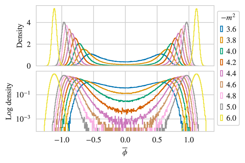
(a)

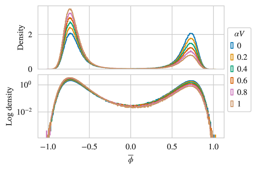
(b)

​

Figure 1: Distribution of $\overline{\phi}$ for LABEL:sub@fig:hmc-hists-M2 fixed $\alpha=0$ varying $m^{2}$ and LABEL:sub@fig:hmc-hists-alpha fixed $m^{2}=-4$ varying $\alpha$, with each histogram estimated using $1.28\times 10^{6}$ samples generated with AHMC.

VI.3 Flow models

For this exploratory study, we study the performance of our training methods applied with a fixed model architecture. We use real NVP flows Albergo et al. (2019); Dinh et al. (2016) constructed from affine coupling layers. Each coupling layer partitions the variables by checkerboarding the sites, and updates one parity of site conditioned on the frozen values of the other parity; successive coupling layers update opposite-parity sites such that all variables are updated once after two layers. As described in Refs. Albergo et al. (2019); Dinh et al. (2016), this partitioned updating scheme is invertible by construction and gives a triangular Jacobian, allowing efficient computation of the Jacobian determinant. In each coupling layer, we use a convolutional neural network to parametrize the affine transformation; compared with fully connected networks, this reduces model size and encodes translational symmetry (up to breaking by the checkerboarding).

The prior distribution used in all cases is an uncorrelated unit-width Gaussian distribution for each component of the scalar field. Each model is constructed from 24 affine coupling layers. The networks parametrizing each affine transformation are made of 4 convolutions with kernel size 5, with leaky ReLU activations (with negative slope = 0.01) after each except the last one, which is followed by a $\tanh$. Each network takes 1 channel as input, gives 2 channels as output, and works with 12 channels at all intermediate stages. Because we are interested in the dynamics of different training schemes, we train each model from scratch, i.e. starting from randomly initialized weights (per PyTorch 1.7 defaults).

We train our models using gradient-based updates with the Adam optimizer Kingma and Ba (2014). Any additional training methods used are noted below where relevant. In some cases, we use gradient norm clipping to stabilize training: after backpropagation, we measure the norm of the gradients before passing them to the optimizer and, if the norm exceeds some threshold value, scale all gradients down by a constant to clip the norm to the threshold. We also employ a step-scheduler in some cases which drops the learning rate by a factor $\gamma=0.5$ every $n$ epochs (typically $n=20$k). Throughout, by one epoch we mean one gradient computation and optimizer step. We train in 32-bit precision, but sample in 64-bit precision to avoid introducing bias due to round-off error compromising invertibility. The average magnetization under the model $\langle\overline{\phi}\rangle_{\tilde{p}}$ computed over each batch of training data serves as a diagnostic of mode collapse. When $\langle\overline{\phi}\rangle_{\tilde{p}}$ and the loss are shown in training histories in the following subsections, they are smoothed by averaging blocks of 25 epochs.

We use a stochastic estimate of the forwards KL divergence to evaluate the quality of approximation of the targets by models trained and constructed by all approaches. This metric quantifies model overlap with the target in a way that is independent of how one uses the models to generate target-distributed samples or otherwise compute expectation values under the target. Using a batch of target-distributed samples generated with augmented HMC, we compute for each model

$$D_{\mathrm{KL}}(p||\tilde{p}) =\int d\phi~{}p(\phi)\log\frac{p(\phi)}{\tilde{p}(\phi)}$$ (21)

$$\approx\frac{1}{N}\sum_{i}\log\frac{p(\phi_{i})}{\tilde{p}(\phi_{i})},\quad(\phi_{i}\sim p)$$

using $\log p=\exp[-S]/Z$ normalized using the stochastic estimator Nicoli et al. (2020b)

$$Z^{-1}\approx\frac{1}{N}\sum_{i}\frac{\tilde{p}(\phi_{i})}{e^{-S(\phi_{i})}},\quad(\phi_{i}\sim p)$$ (22)

so that $D_{\mathrm{KL}}=0$ when $p=\tilde{p}$. For each set of action parameters (i.e. each target distribution), we evaluate $D_{\mathrm{KL}}$ using a single shared ensemble of AHMC validation data consisting of $N=10^{6}$ samples, enabling direct comparisons with perfectly correlated sampling noise between different models of the same target. We use a shared value of $Z$ to normalize $p$ for each set of parameters, computed using models trained with AHMC data and not accounting for the error in this estimate.

During training we assess whether model quality has converged using a finite-sample estimator of the effective sample size (ESS) per configuration Kish (1965); Martino et al. (2017),

$$\text{ESS}/N\approx\frac{1}{N}\frac{(\sum_{i}w_{i})^{2}}{\sum_{i}w_{i}^{2}},\quad(\phi_{i}\sim\tilde{p})$$ (23)

where $w_{i}\equiv p(\phi_{i})/\tilde{p}(\phi_{i})$. The estimator is constructed such that the normalization of $w_{i}$ cancels in the ratio, allowing evaluation using $\exp[-S(\phi)]$ in place of $p(\phi)$. Throughout this section, the ESS presented in plots of training histories is measured every 25 epochs on a batch of 16000 samples unless noted otherwise. We diagnose convergence of training based on when the envelope of this (noisy) estimator has approximately plateaued. In the discussion below we occasionally use this finite-sample metric as a rough measure of the quality of overlap of a model on to a target. However, this measure should be interpreted cautiously given the discussion in Sec. VII, where we find the asymptotic ESS is near zero for many of these models. We defer further discussion of how different metrics of model quality relate to (problems with) the asymptotic performance of flow-based MCMC until Sec. VII.

In this proof of principle study, we do not perform any systematic study of the dependence of results on the model architecture, the random seed (which determines both initial model parameters and the generated training datasets), or repeatability in training. These factors represent a possibly large source of unquantified systematic error in all presented metrics of model quality. Despite these sources of systematic error, we are able to determine qualitative and certain quantitative features of the results that are expected to be robust.

VI.3.1 Reverse KL self-training

We first examine the behavior of reverse KL self-training when applied to targets in the broken symmetry phase, both to provide concrete demonstrations of the problem of mode collapse and to establish a baseline for the difficulty of training a model which correctly captures the bimodal distribution of the theory of interest.

Figure 2 shows a training history for a model targeting $m^{2}=-3.6$ and $\alpha=0$. Figure 1a shows that the target distribution for these parameters is bimodal but the modes still overlap substantially. We see in the running estimate of $\langle\overline{\phi}\rangle_{\tilde{p}}$ shown in Fig. 2 over the course of training (computed on raw model outputs, without applying reweighting or Metropolis accept/reject steps) that the model is initially heavily biased towards one mode, but slowly and gradually learns to evenly weight the two modes.

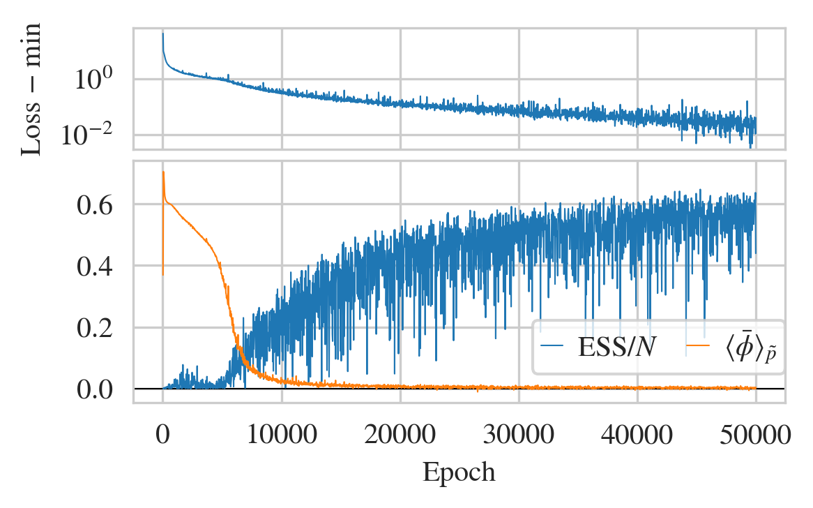
Figure 2: Reverse KL training history exhibiting smooth approach from unimodal to bimodal, for a flow model targeting $m^{2}=-3.6$ and $\alpha=0$, trained with batch size 16000.

In the opposing regime, Fig. 3 shows a training history for the case where $m^{2}=-5$, where the two modes are well-separated. The model quickly trains into a unimodal distribution. The apparently high finite-sample ESS for the mode-collapsed model suggests that it is a good fit to the collapsed-upon mode. Given sufficient training, the model may eventually have converged towards a bimodal distribution, but it was not found to do so in the long (though finite) training time used here.

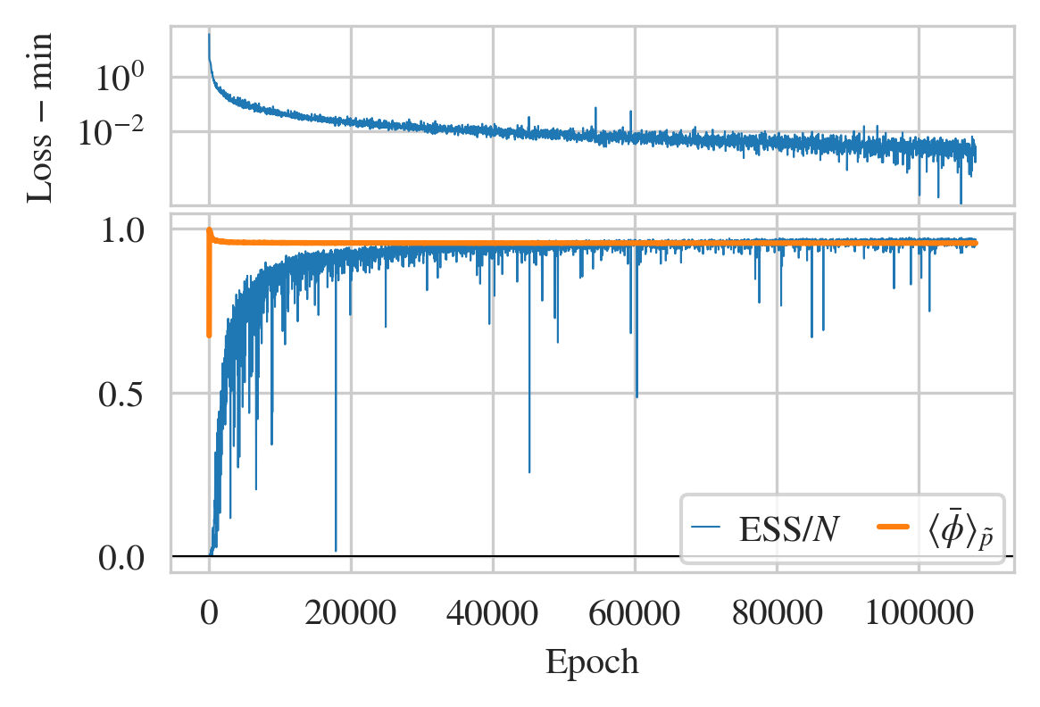
Figure 3: Reverse KL training history exhibiting mode collapse, for a flow model targeting $m^{2}=-5$ and $\alpha=0$, trained with batch size 16000. The similar values of $\text{ESS}/N$ and $\langle\overline{\phi}\rangle_{\tilde{p}}$ are coincidental.

Figure 4 presents a training history for a model targeting $m^{2}=-4$ and $\alpha=0$, demonstrating interesting behavior in the borderline regime between the two extremes discussed above. The model initially learns to sample from a unimodal distribution, which can be seen in Fig. 4 in that $\langle\overline{\phi}\rangle_{\tilde{p}}\neq 0$ at early times. However, around epoch 15k the model begins to become sensitive to the other mode and at epoch $\approx 22000$, the model tunnels suddenly to a bimodal distribution with $\langle\overline{\phi}\rangle_{\tilde{p}}\approx 0$. The loss drops as this occurs, consistent with the bimodal distribution being the true minimum of the reverse KL divergence. Note that, unlike the previous cases, this training used (aggressive) gradient norm clipping; without it, the model stochastically tunnels between unimodal and bimodal before eventually settling into the bimodal distribution after $\approx(100-150)\times 10^{3}$ epochs.

Figure 4: Reverse KL training history exhibiting tunneling from unimodal to bimodal, for a flow model targeting ${m^{2}=-4}$ and $\alpha=0$, training with batch size 16000 and using gradient norm clipping.

For these simple systems, we find that for $\alpha=0$ and $-m^{2}\leq 4$, reverse KL self-training produces a bimodal distribution in a tractable amount of time with behavior like that of either Fig. 2 or 4. Similarly, reverse KL training produces a bimodal distribution for all of the values of $\alpha$ we consider at fixed $m^{2}=-4$, likely because models could be trained for $m^{2}=-4$ and $\alpha=0$, and the other choices of $\alpha$ used here do not significantly perturb the modal structure. We have seen that we can (slightly) extend the reach of reverse KL self-training using tools like gradient norm clipping and decaying learning rates, so it may be possible to push further into the broken regime with improved training.

It is interesting to note that for $\alpha\neq 0$ we observe that the models collapse onto the lower-weight mode of the target distribution at positive $\overline{\phi}$ in early training more frequently than physical reasoning would suggest, in ${\gtrsim 50\%}$ of training runs. This suggests that our architecture biases the model towards the positive-$\overline{\phi}$ peak.

VI.3.2 Mixture models

In order to construct a mixture model which is a good approximation to some target distribution, we need a set of component models which together provide good coverage of the target: at least one model should have nontrivial density everywhere the target has significant support. In the previous section we saw that reverse KL self-training is not effective at training samplers for bimodal distributions when the modes of the target are well-separated. However, the apparently high finite-sample ESS for mode-collapsed models indicate that they are good fits to the collapsed-upon modes. They are thus good candidates for mixture components in single-model mixtures as described in Sec. IV.

In the symmetric $\alpha=0$ case, the two modes of the target distribution are identically shaped, so a model for one mode can serve equally well as a model for the other. Thus, rather than training separate models for each mode, we use a single model to construct a symmetrized mixture as discussed in Sec. IV.2. The relevant set of transformations are the global $Z_{2}$ under which $\phi\rightarrow\phi^{\prime}=t\phi$ with $t\in\{1,-1\}$. Specializing Eqn. (11) to this case, the density of the mixture is

$$\tilde{p}^{(\text{symm})}_{\text{mix}}(\phi)=\frac{1}{2}\left[\tilde{p}(\phi)+\tilde{p}(-\phi)\right].$$ (24)

Figure 5 compares the distribution of $\overline{\phi}$ from a mode-collapsed model to the distribution for a symmetrized mixture constructed from it; as expected, the mixture distribution fits the peaks very well, but is undersupported in the region between the modes.

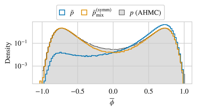
Figure 5: Distribution of $\overline{\phi}$ for samples drawn from a unimodal model ($\tilde{p}$) and from a symmetrized mixture model constructed from it ($\tilde{p}_{\text{mix}}^{(\text{symm})}$), both for $m^{2}=-4$ and $\alpha=0$. The mixture samples are generated by postprocessing the samples shown for the unimodal model. Note: these histograms are computed using raw model samples, and no statistical corrections have been applied. The target distribution ($p$), as measured using AHMC, is shown for comparison.

For the explicitly broken $\alpha\neq 0$ case, we may use a symmetrized mixture model without any formal issues; this will simply result in poor overlap with the target when the relative weights of the modes of the target are too dissimilar. For the range of $\alpha$ we consider here, we observe (cf. Fig. 1b) that while the relative weights of the modes become increasingly tilted, the shapes of the modes remain similar. This can be treated with a straightforward generalization of the symmetrized mixtures, wherein we randomly apply a sign with probability $p_{\text{flip}}\neq 0.5$. The mixture is thus over the original flow model with weight $1-p_{\text{flip}}$, and the flow model composed with a sign flip with weight $p_{\text{flip}}$; the mixture density is

$$\tilde{p}^{(\text{tune})}_{\text{mix}}(\phi)=(1-p_{\text{flip}})\tilde{p}(\phi)+p_{\text{flip}}\tilde{p}(-\phi).$$ (25)

We emphasize that $\phi$ in the above equation should be read as the $\phi$ obtained after applying the random sign. Here, $p_{\text{flip}}$ is a parameter which can be tuned to maximize some measure of quality of the model. We optimize $p_{\text{flip}}$ by minimizing the reverse KL divergence on a fixed sample of $10^{6}$ configurations drawn from the component model, fixing the draw used to determine whether a sign flip is applied to each configuration.

In Sec. IV.3 we present a construction where the mixture weights are adaptively set using information from the target distribution rather than left as tunable parameters. Applied to the $Z_{2}$ transformations relevant to the scalar lattice theory, we can sample from an adaptive mixture by first drawing a sample $\varphi$ from our flow model, then randomly applying a minus sign with probability $p(-\varphi)/[p(\varphi)+p(-\varphi)]$ to produce $\phi=\pm\varphi$. In the symmetric $\alpha=0$ case where $p(\varphi)=p(-\varphi)$ this reduces to a symmetrized mixture. Away from this limit, we can specialize Eqn. (13) to obtain the density of the final sample,

$$\tilde{p}^{(\text{adapt})}_{\text{mix}}(\phi)=\frac{p(\phi)}{p(\phi)+p(-\phi)}\left[\tilde{p}(\phi)+\tilde{p}(-\phi)\right].$$ (26)

Figure 6 compares the forwards KL divergence of these different constructions at fixed $m^{2}=-4$ varying $\alpha$ (all three mixture constructions coincide when $\alpha=0$). At lower values of $\alpha$ where the distribution is more symmetric, all three methods perform roughly equivalently. As $\alpha$ grows and the distribution becomes more asymmetric, the adaptive mixtures and mixtures with tuned $p_{\text{flip}}$ remain approximately the same, while the symmetrized mixture becomes an increasingly poor approximation of the target. Adaptive mixtures perform nearly identically with mixtures with tuned $p_{\text{flip}}$, without the need to optimize any mixture parameters. The slight peak at $\alpha V=0.2$ is most likely a training effect. As mentioned above, for all $\alpha$ we consider, reverse training eventually finds the bimodal distribution. In fact, the models begin to move towards bimodal early on, compromising the available quality of unimodal models (cf. the drop in ESS in Fig. 4 around epoch 10k). Further study at parameters deeper in the bimodal phase could provide cleaner results, but the relative performance of the different approaches is clear. Figure 7 compares the distributions of $\overline{\phi}$ resulting from applying the three different methods at $\alpha=0.8/V$; the symmetric mixture overweights the lower peak, while adaptive mixtures and mixtures with tuned $p_{\text{flip}}$ produce similar distributions with the correct relative mode weights.

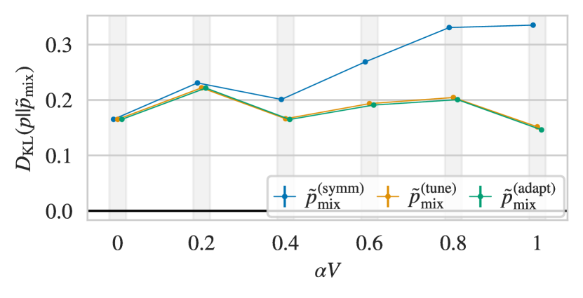
Figure 6: Forwards KL divergence (lower indicates better agreement) for the three different mixture model constructions described in the text, estimated using shared ensembles of $10^{6}$ target samples, for fixed $m^{2}=-4$ and varying $\alpha$. At each $\alpha$, all three mixtures are constructed from the same unimodal component model, obtained using reverse KL self-training. Errors are computed by bootstrapping, and are smaller than the markers for all points. Additional variance due to seed dependence is not quantified.

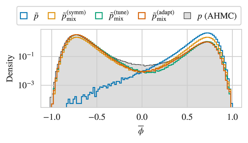
Figure 7: Distribution of $\overline{\phi}$ for samples drawn from a unimodal model ($\tilde{p}$), as well as various different mixtures constructed from it ($\tilde{p}_{\text{mix}}^{(\ldots)})$ as described in the text, all for $m^{2}=-4$ and $\alpha V=0.8$. The mixture samples are generated by postprocessing the samples shown for the unimodal model. Note: these histograms are computed using raw model samples, and no statistical corrections have been applied. The target distribution ($p$), as measured using AHMC, is shown for comparison.

VI.3.3 Forwards KL training

As discussed in Sec. V.1, we can implement a self-training scheme using the forwards KL divergence by generating a training dataset using the model itself, then reweighting to correct for the mismodeling of the target distribution. This approach allows us to augment the training data in a way is not structurally possible when using reverse KL self-training.

We first examine the behavior of reweighted forwards KL self-training without any augmentation of the training data. Figure 8 shows a typical training history for this approach, applied to the parameters $m^{2}=-5$ and $\alpha=0$ where the modes are well-separated. As with reverse KL self-training, the model collapses onto one of the modes, indicating that mode collapse is a problem of self-training schemes in general and not a specific feature of reverse KL self-training.

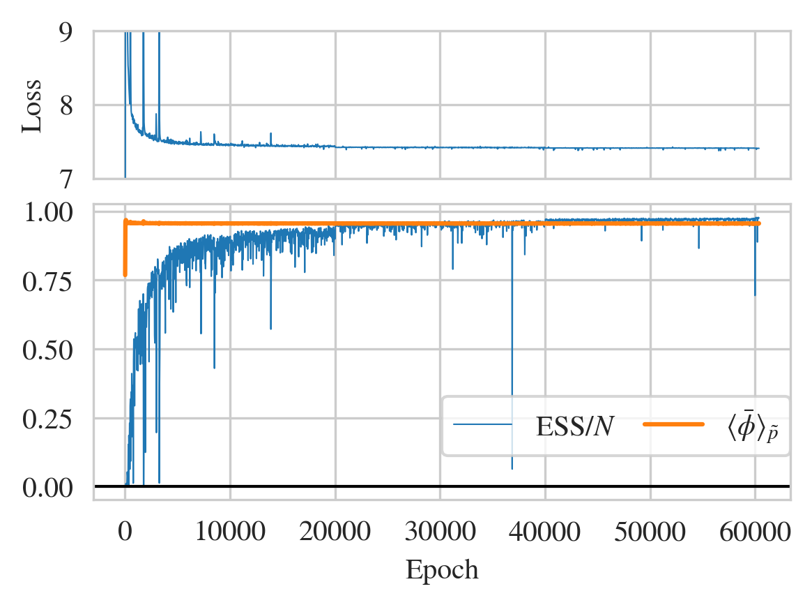
Figure 8: Reweighted forward KL self-training history exhibiting mode collapse, for a flow model targeting $m^{2}=-5$ and $\alpha=0$, training with batch size 16000, using gradient norm clipping, and with the learning rate dropping by a factor of $\gamma=0.5$ every 20000 epochs. The similar values of $\text{ESS}/N$ and $\langle\overline{\phi}\rangle_{\tilde{p}}$ are coincidental.

To improve over reverse KL self-training we must take advantage of the ability to augment the training dataset, which we do by generating each batch of training data by constructing and sampling from a single-model mixture using the flow model being trained. We first examine the symmetric $\alpha=0$ case where all of the mixture constructions we consider in this work are equivalent. Figure 9 shows a training history for a model trained using this scheme, targeting $m^{2}=-4$ and $\alpha=0$. Over the course of training, $\langle\overline{\phi}\rangle_{\tilde{p}}\approx 0$ up to per-epoch fluctuations, indicating that the model trains directly into a bimodal distribution. This is dissimilar to the training dynamics observed in e.g. Fig. 4 with reverse KL self-training at these parameters, where the model initially collapses onto a single mode then eventually finds the bimodal distribution.

We generically observe similar training dynamics with this scheme as with reverse KL self-training for unimodal models, except for an extra instability that must be regulated with gradient norm clipping. The large gradients that destabilize training and necessitate clipping likely arise in part from batches where a single high-weight configuration (like those discussed in Sec. VII) dominates the reweighted loss estimate. We also observe that the value of $\langle\overline{\phi}\rangle_{\tilde{p}}$ for the model distributions can fluctuate at late times, but we find that step-scheduling the learning rate (i.e. reducing the learning rate by a factor $\gamma=0.5$ every 20000 epochs) regulates this effect and allows $\langle\overline{\phi}\rangle_{\tilde{p}}$ to settle to zero (or the appropriate nonzero value, in the asymmetric $\alpha\neq 0$ case).

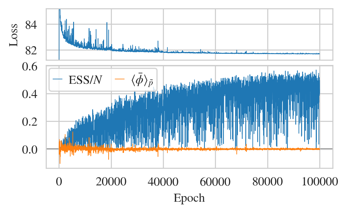
Figure 9: Reweighted forward KL self-training history (with training data sampled from a mixture) exhibiting direct training to bimodal, for a flow model targeting $m^{2}=-4$ and $\alpha=0$, training with batch size 16000, using gradient norm clipping, and with the learning rate dropping by a factor of $\gamma=0.5$ every 20000 epochs.

We also test the training scheme using the naive data augmentation described in Sec. V.1, where rather than sampling from a mixture we simply apply a random sign flip to each configuration. In this case, the reweighting factors use $p^{\prime}=\tilde{p}$ for the configurations before negation, while $\log\tilde{p}$ in the loss is computed after negation. We observe similar training dynamics for this scheme as when using training data sampled from a mixture. We compare models with those obtained using other forwards KL approaches below.

To set a baseline for the self-training approaches, we train models using data generated on-the-fly using augmented HMC, providing a theoretically infinite training dataset as in self-training schemes. This training dataset amounts to a limiting-case perfect dataset for reweighted forwards KL self-training: all reweighting factors are equal so no statistical power is lost, and due to the augmentation the training data is guaranteed to encode the appropriate relative mode weights. Specifically, for a given batch size $B$, we generate our training dataset by running $B$ completely independent AHMC chains (taking advantage of GPU parallelism), initially equilibrating each for 1000 trajectories. For every epoch of training, we advance all $B$ chains by 10 trajectories to produce a new training dataset for each epoch. We use identical AHMC settings as those discussed in Sec. VI.2. Autocorrelations within each chain are minimal for these settings, so each batch of training data is approximately independent from the last.

Figure 10 compares the forwards KL divergences for models obtained using self-training schemes and training with AHMC data in the $\alpha=0$ case as a function of $m^{2}$. For most parameters, including those deep in the bimodal phase, all methods perform comparably, with self-training producing only marginally poorer models than training with AHMC data. The approximate self-training scheme with naive data augmentation performs comparably to drawing training data from a mixture.

As shown in Fig. 11, we observe that the final quality of self-trained models depends significantly on the batch size used for training, even when training to convergence. The dependence is weak, if present at all, for models trained with AHMC data. It is unclear whether self-trained model quality will converge to AHMC-trained model quality in the limit of infinite training batch sizes. For sufficiently large batch sizes, the naive data augmentation scheme appears to produce equivalently good models as the mixture scheme. This batch size dependence is stronger than what we have observed using reverse KL self-training on unimodal distributions.

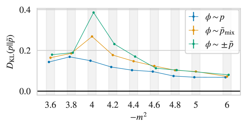
Figure 10: Forwards KL divergence (lower indicates better agreement) for models trained using different versions of forwards KL training, estimated using shared ensembles of $10^{6}$ target samples, for fixed $\alpha=0$ and varying $m^{2}$. The label $\phi\sim p$ denotes models trained using data generated by AHMC, $\phi\sim\tilde{p}_{\mathrm{mix}}^{(\text{symm})}$ denotes models self-trained using samples from a symmetrized mixture, and $\phi\sim\pm\tilde{p}$ denotes models self-trained using samples naively augmented by applying a random sign. All models are trained with batch size 16000 and using gradient norm clipping. Errors are computed by bootstrapping, and are smaller than the markers for all points. Additional variance due to seed dependence is not quantified.

Figure 11: Forwards KL divergence as a function of batch size for models trained using different versions of forwards KL training for $\alpha=0$ and $m^{2}=-4$, estimated using shared ensembles of $10^{6}$ target samples. Errors are computed by bootstrapping, and are smaller than the markers for all points. Additional variance due to seed dependence is not quantified.

As discussed above, when $\alpha\neq 0$ we can consider several in-principle different mixture model constructions. To augment the data for forwards KL self-training, we only investigate the performance of symmetrized mixtures (where we apply a sign to each sample with ${p_{\text{flip}}=0.5}$, regardless of the relative weights of the modes of the target) and adaptive mixtures. The mixture construction with tunable $p_{\text{flip}}$ is difficult to apply in this context: during training the flow models will in general be bimodal, so $p_{\text{flip}}$ is not directly related to the relative mode weights as it is with mixtures of unimodal models, and the relative mode weights change quickly, meaning the optimal choice of $p_{\text{flip}}$ depends on the current state of the model. Exploring these complications is beyond the scope of the present study. We also test the naive data augmentation scheme for $\alpha\neq 0$, fixing the probability of negating each configuration to $p_{\text{sign}}=0.5$ to avoid the same complications as in the tuned $p_{\text{flip}}$ mixture.

Figure 12 compares models self-trained using symmetrized and adaptive mixtures, along with models trained with AHMC samples and the naive data augmentation scheme, for $\alpha\neq 0$. The discrepancy between AHMC-trained results and self-trained results extends to non-zero $\alpha$. The two different mixture approaches perform comparably, although the results of using adaptive mixtures have more variance, suggesting less stable training or stronger seed dependence. The success of the symmetrized mixture scheme implies that the loss of statistical power from reweighting to correct the mode weights is not a large effect. The naive data augmentation scheme performs generically worse than the mixtures (although comparing with Fig. 12, $m^{2}=-4$ is a particularly poor set of parameters for this scheme), and predictably produces models of increasingly poor quality as $\alpha$ increases and $p_{\text{sign}}=0.5$ becomes a poor approximation.

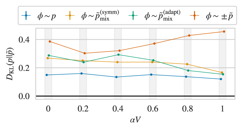
Figure 12: Similar to Fig. 10, but with fixed $m^{2}=-4$ and varying $\alpha V$. Additional variance due to seed dependence is not quantified, but training using data from symmetrized ($\phi\sim\tilde{p}^{(\text{symm})}_{\text{mix}}$) and adaptive ($\phi\sim\tilde{p}^{(\text{adapt})}_{\text{mix}}$) mixtures are identical procedures at $\alpha=0$, so the discrepancy reflects seed dependence in that case.

VI.3.4 Adiabatic retraining & flow-distance regularization

As introduced in Secs. V.2 and V.3, both adiabatic retraining and flow-distance regularization can be thought of as reverse KL self-training with an adiabatically changing the loss function, so we discuss them together.

For adiabatic retraining, we tune the action parameter $m^{2}$ over the course of training via a schedule function $g(t)\in[0,1]$ so that the effective instantaneous $\phi^{4}$ action can be explicitly written as

$$S_{\text{inst}}(\phi;t)=S_{E}(\phi)+g(t)\frac{1}{2}(m_{0}^{2}-m^{2})\sum_{x}\phi(x)^{2}$$ (27)

where $S_{E}$ is given by Eqn. (19). When targeting the symmetric potentials where $\alpha=0$, the initial parameter $m_{0}^{2}=-3$ is chosen to correspond to a unimodal distribution to serve as the starting point of the adiabatic training. For flow-distance regularization, each configuration $\phi$ contributes to the loss as

$$L(\phi,p)=\log\tilde{p}+S_{E}(\phi)+\kappa g^{\prime}(t)\sum_{x}(\phi(x)-z(x))^{2}$$ (28)

where $L(\tilde{p},p)=\frac{1}{N}\sum_{i}L(\phi_{i},p)$ and $g^{\prime}(t)\in[0,1]$ is a schedule function. The hyperparameter $\kappa$ sets the initial relative contributions of the regularizer term and the action. In practice, we find that both training processes are more stable if we take the schedule functions $g(t),g^{\prime}(t)$ to be concave functions of $t$ rather than linear interpolations. We use the schedules

$$g(t)=g^{\prime}(t)=\frac{e^{-k\frac{t-t_{1}}{t_{2}-t_{1}}}-e^{-k}}{1-e^{-k}},\quad t_{1}<t\leq t_{2}$$ (29)

choosing $t_{1},t_{2},k$ appropriate to each problem. The schedule is defined to be flat before $t_{1}$ so that initially, adiabatic retraining trains a model appropriate to the initial parameters before beginning to interpolate, and flow-distance regularization trains a model close to the identity before the regulator begins to be removed.

In the symmetric case where $\alpha=0$, for $m^{2}=-4$ both approaches successfully train bimodal flow models using the schedule parameters in Table 1. When the schedule moves too quickly, the models tend to suddenly collapse into a unimodal distribution during training, so increasingly slow tuning is required as $m^{2}$ becomes more negative. We were able to increase the reach of these training schemes without using impractically slow schedules by “rewinding” when mode collapse occurs by reloading a recent checkpoint and, if necessary, lowering the learning rate. We have had mixed success either reloading the optimizer state or resetting the optimizer parameters when rewinding. Gradient norm clipping can help make training more robust against collapse but does not prevent it entirely.

Method	Coupling strength	$t_{1}$	$t_{2}$	$k$
Adiabatic retraining	$m_{0}^{2}=-3.0$	40000	120000	1
Flow-distance	$\kappa\approx 0.1$	20000	120000	1

Table 1: Example schedule parameters for adiabatic retraining and flow-distance regularization, for parameters $m^{2}=-4$ and $\alpha=0$.

With the caveat that any interpretation based on the finite-sample ESS estimator may be unreliable given the slow convergence problems discussed in Sec. VII below, we proceed with an analysis of the training dynamics of these methods.

Figure 13 shows the training history of a model for $m^{2}=-4$ trained using flow distance regularization with the parameters in Table 1 and a decaying learning rate. During the initial regulator-dominated part of training when $t<t_{1}$, the loss converges and the magnetization $\langle\overline{\phi}\rangle_{\tilde{p}}$ goes to zero. The finite-sample ESS is near zero, indicating poor overlap with the target, as expected for a model which has converged to a prior-like distribution. As the regulator is slowly removed, the loss changes smoothly, the ESS increases slowly, and the magnetization remains near zero, indicating that the model is not mode collapsed. After the regulator is removed, the envelope of the ESS is nearly flat (possibly increasing slowly), indicating that the training schedule finds a nearly converged model without additional unregulated training. Fluctuations in $\langle\overline{\phi}\rangle_{\tilde{p}}$ under additional training are damped by the decaying learning rate.

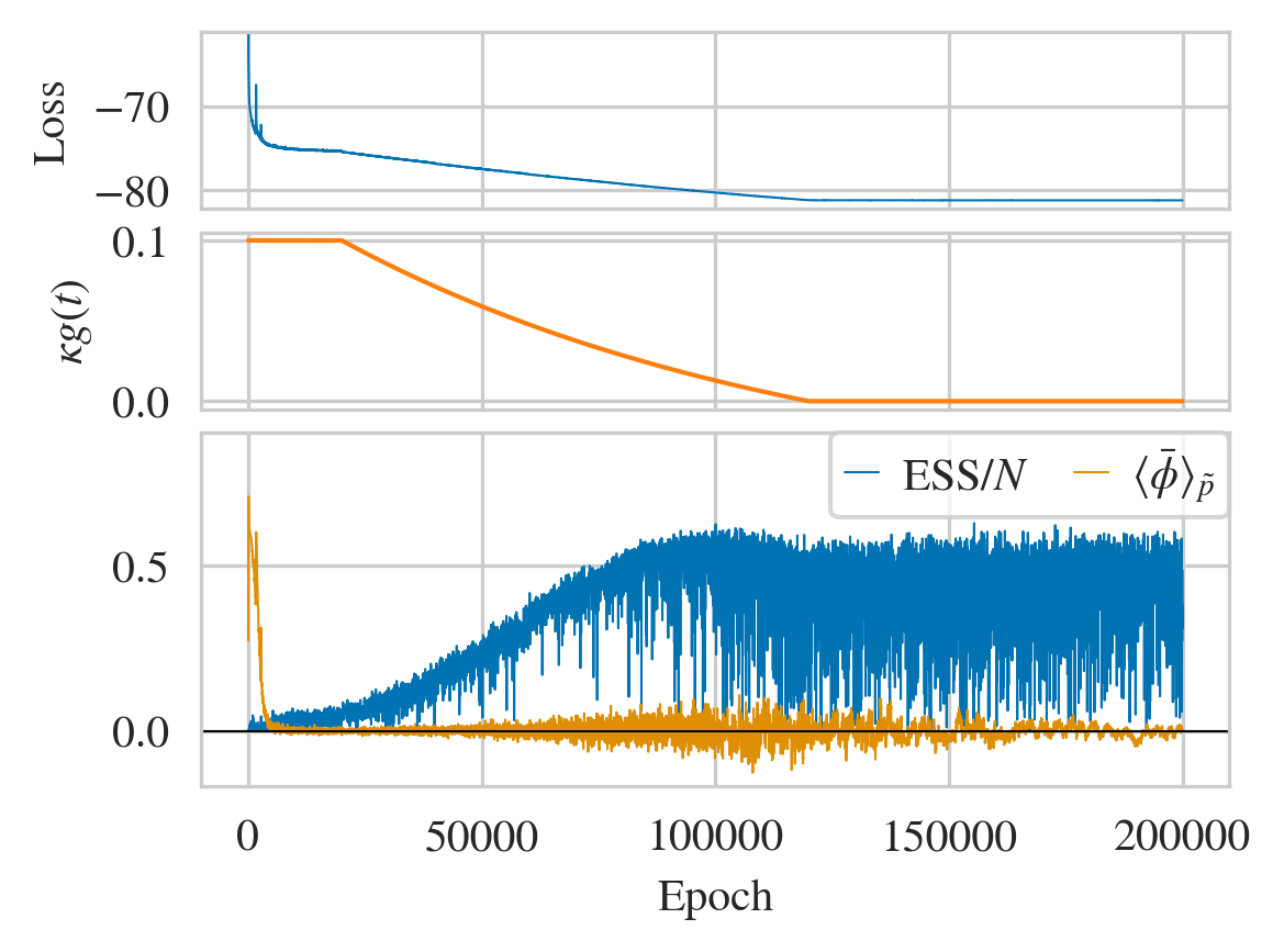
Figure 13: Training history for flow-distance regularization, for a flow model targeting $m^{2}=-4$ and $\alpha=0$, training with batch size 1000. The learning rate starts from $10^{-3}$ and drops by a factor of $\gamma=0.5$ every 20000 epochs.

Figure 14 shows the training history of a model for $m^{2}=-4$ trained using adiabatic retraining with the schedule parameters in Table 1. During the initial phase of training before $t_{1}$, the model learns a nontrivial approximation of the instantaneous target with $m^{2}=-3$ as indicated by the loss and by the ESS onto the instantaneous target (orange), although it has not yet asymptotically converged before the schedule begins to be tuned. The ESS onto the final target $m^{2}=-4$ (blue) is near zero, as expected given the different initial and final target distributions. As the action is tuned towards $m^{2}=-4$, the loss changes smoothly and $\langle\overline{\phi}\rangle_{\tilde{p}}$ remains near zero up to per-epoch fluctuations, indicating that the model does not collapse onto a single mode. Similar to Fig. 13, the ESS onto the final target $m^{2}=-4$ increases slowly as the model becomes an increasingly good approximation of the target. The increasing variance in the magnetization $\langle\overline{\phi}\rangle_{\tilde{p}}$ and the change in ESS after the schedule reaches $m^{2}=-4$ reflect that the interpolation is not fully adiabatic, although this interpretation is confounded by the interpolation beginning with a model which is not asymptotically converged (i.e. stable under further training). The apparent drop in the ESS under additional training after the schedule reaches $m^{2}=-4$ may suggest that the scheme produces transiently better models than can be achieved by direct training.

On the other hand, the finite-sample ESS onto the instantaneous target in Fig. 14 changes smoothly over the course of adiabatic retraining; the decrease reflects the fixed architecture’s decreasing ability to represent the increasingly complicated target. The nontrivial overlap with all instantaneous targets throughout training suggests that the initial expense of training a model from a random initialization could be amortized over different action parameters, which could help circumvent possible issues with the scaling of the costs of training flow models Del Debbio et al. (2021).

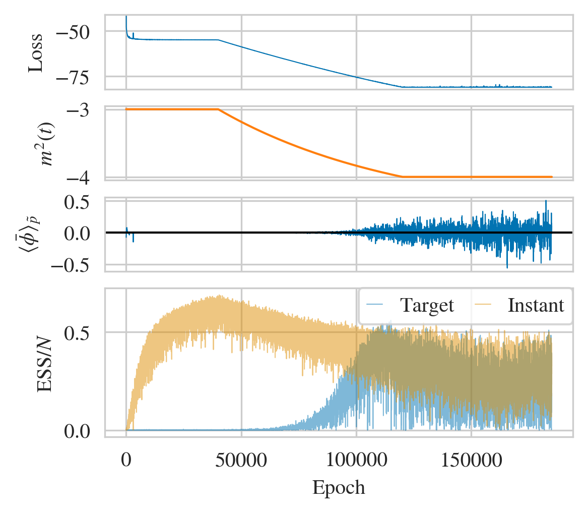
Figure 14: Training history for adiabatic retraining, for $\alpha=0$ and interpolating from the initial $m_{0}^{2}=-3$ to the final target $m^{2}=-4$ as described in the text, training with batch size 4000. In the bottom panel, “Target” indicates ESS$/N$ for reweighting to the final action with $m^{2}=-4$, while “Instant” is for reweighting to the current instantaneous action with $m^{2}(t)$ as shown in the second panel. The target ESS is evaluated on 16000 configurations every 25 epochs. The instantaneous ESS is evaluated every epoch, and smoothed by averaging over blocks of 4 epochs so that it incorporates the same number of samples as the target ESS; the resulting metrics are nevertheless inequivalent and the instantaneous ESS is expected to be more positively biased due to the smaller sample size.

Both schemes are applicable to explicitly broken potentials with $\alpha\neq 0$. Flow-distance regularization can be used to train directly into the bimodal target just as in the $\alpha=0$ case, although we find that for potentials with larger tilts, the model is more likely to collapse to unimodal and usually needs a slower schedule. For adiabatic retraining, we observe that the particular trajectory through action parameter space is important, specifically that avoiding mode collapse requires training into a bimodal distribution before training towards a target with explicitly broken symmetry.

VI.4 Comparison

Figures 15 and 16 show the distributions of $\overline{\phi}$ for $\alpha=0$ and $\alpha=0.8/V$, respectively, for models constructed using the different approaches of Secs. IV and V. As advertised above, all methods produce models that sample from both peaks of the bimodal distribution for these two sets of parameters. Reverse KL self-training produces a model that severely underweights the region between the modes in Fig. 15, but not in Fig. 16, indicating that this is not a generic effect. Flow distance regularization uniquely produces models that do not underweight the inner region, suggesting that it reduces the initial overconcentration on peaks described in Sec. II.4. All other models only mildly underweight the inner region.

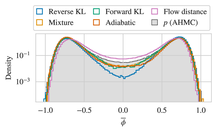
Figure 15: Distribution of $\overline{\phi}$ for models constructed using the different approaches, for $m^{2}=-4$ and $\alpha=0$. Note: these histograms are computed using raw samples from the model distribution, and no statistical corrections have been applied. The distribution of $\overline{\phi}$ for the target distribution $p$, estimated using AHMC, is underlaid in gray for ease of comparison.

Figure 16: As for Fig. 15, but for $m^{2}=-4$ and $\alpha=0.8/V$.

Figure 17 shows the forwards KL divergences of models constructed using the various different approaches described here. Without accounting for systematic uncertainties due to differences in training details and initialization dependence, we cannot robustly evaluate the relative capabilities of the different methods presented, and being fully conservative can only state that all methods produce bimodal models with nontrivial, roughly comparable overlap with the targets. However, with this caveat understood, we can attempt a more detailed analysis.

Although bimodal models can be obtained using reverse KL self-training if the modes of the target distribution are not too separated, Fig. 17a suggests that overlap with the target suffers as the distribution becomes more bimodal. We can attribute the high variance in the quality of reverse KL self-trained models in Fig. 17b to training details and seed dependence; comparing Figs. 15 and 16, we see that different reverse KL self-training runs yield (after training to convergence) models with different support relative to the target in the inner tails.

Conversely, the quality of mixture models, as well as models trained using them in the reweighted forwards KL self-training scheme, appears to improve as the target becomes increasingly bimodal. Mixtures generally yield the lowest divergence for highly bimodal symmetric targets with $m^{2}<-4$ in Fig. 17a, and comparable performance to the forwards KL trained models for $m^{2}=-4$ and $\alpha\neq 0$ in Fig. 17b. The reduced performance of mixtures at $m^{2}=-4$ compared with that for more bimodal targets is due to the lack of availability of high-overlap unimodal models, as the models quickly begin to move towards the bimodal distribution under reverse KL self-training at these parameters (as seen in Fig. 4). Similarly, the counterintuitive underperformance of some of the mixtures at larger $\alpha$ in Fig. 17b versus reverse KL self-trained bimodal models is due to what amounts to differences in stopping criteria: unimodal models in the presented mixtures are necessarily taken from earlier in reverse KL self-training runs that eventually produce bimodal models, and comparing Figs. 5 and 7 we see that some “unimodal” models have more support on the missed peak than others, indicating that some mixture components have been trained further towards finding the bimodal distribution.

As discussed above, for forwards KL training, we observe worse overlap with the target for self-trained models than with models trained with AHMC data. However, forwards KL self-training with mixture samples typically produces models at least as good as reverse KL self-trained ones, and does so while training directly into the bimodal distribution without needing to wait for the model to stochastically tunnel to bimodal as with reverse KL. Forwards KL self-training thus provides a reliable means of more efficiently training bimodal distributions, especially for highly bimodal targets where it is unclear that reverse KL will find the bimodal distribution in any tractable amount of time, given that we have sufficient knowledge of the target’s mode structure to augment the training data.

Adiabatically retrained and flow-distance regulated models appear to have worse overlap than those produced by the other methods; however, this may be due purely to differences in training details necessitated by the less-robust adiabatic training schemes, such as differences in stopping criteria as well as the rewinding procedure described above. In Fig. 17a we observe that flow-distance regularization appears to produce models with worse overlap as the target becomes more bimodal, but the same is not true for adiabatic retraining. Further investigation is required to disambiguate whether the declining quality for flow-distance regularization is due purely to training details, or if the initial training targeting a (unimodal) prior-like distribution produces a model inflexible to further training into the (bimodal) target. Nonetheless, the practical difficulties of tuning these methods to effectively produce bimodal distributions for this theory suggest that it may be easier to work with other methods of producing bimodal flow models, when they are available.

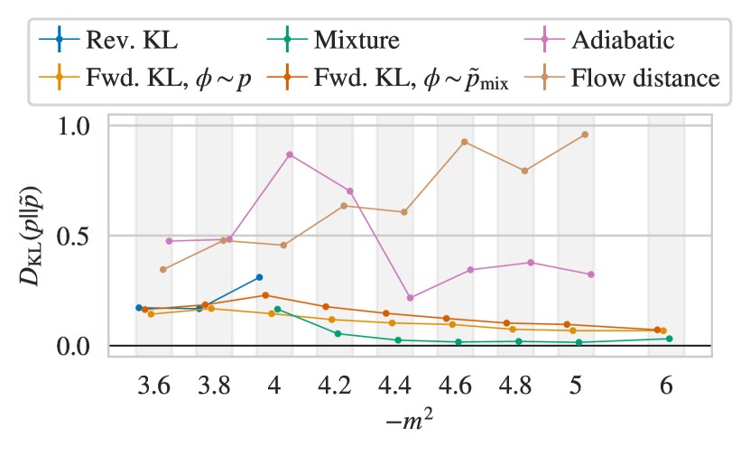
(a)

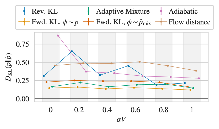
(b)

​

Figure 17: Forwards KL divergence (lower indicates better agreement) for models constructed using the different approaches described in the text, for LABEL:sub@fig:cf_fkl_M2 fixed $\alpha=0$ and varying $m^{2}$ and LABEL:sub@fig:cf_fkl_alpha fixed $m^{2}=-4$ and varying $\alpha$, estimated using shared ensembles of $10^{6}$ target-distributed samples. Errors are computed by bootstrapping, and are smaller than the markers for all points. Additional variance due to seed dependence is not quantified. Missing points indicate that we were unable to obtain models for those parameters using the corresponding method.

VII Sampling using multimodal models in scalar field theory

In this section, we examine the utility of the models described above in generating target-distributed samples using both flow-based MCMC and a composite algorithm which mixes updates using HMC and flow-based MCMC. We find that, when used with flow-based MCMC, these models generically produce pathologically inefficient samplers due to undersampling in the inner tails. The way this issue arises is subtle, so we note its effects in various direct checks of sample quality and discuss how it can be better diagnosed using target-distributed validation data. To demonstrate its severity, we perform a case study of the asymptotic performance of flow-based MCMC using an example model. Finally, we demonstrate that the problems of flow-based MCMC can be regulated by augmenting with HMC to produce an efficient composite MCMC sampler.

VII.1 Flow-based MCMC

Figure 18 shows the flow-based MCMC acceptance rate for models constructed using the different approaches presented in this work, modeling the variance in acceptance rate for different model-generated datasets by applying Independence Metropolis (as described in Sec. II.3) to different bootstrap draws from a fixed sample of $10^{6}$ configurations. The resulting estimates have little error, and all models yield samplers with acceptance rates $\sim 30\%-90\%$, with the acceptance rate ordering models similarly to the forwards KL divergence in the previous section.

(a)

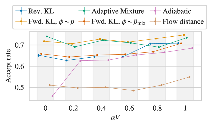
(b)

​

Figure 18: MCMC acceptance rate for models constructed using the different approaches described in the text, for LABEL:sub@fig:cf_ar_M2 fixed $\alpha=0$ and varying $m^{2}$ and LABEL:sub@fig:cf_ar_alpha fixed $m^{2}=-4$ and varying $\alpha$. All estimates are made on $10^{6}$ model-distributed samples, with errors computed by taking bootstrap draws from fixed datasets and applying independence Metropolis within each. Error bars are smaller than the markers for all points. Additional variance due to seed dependence is not quantified.

Figures 19 and 20 show histograms of $\overline{\phi}$ for $m^{2}=-4$ and $\alpha=0$ and $0.8/V$, respectively, with each constructed from $10^{6}$ target-distributed samples generated using flow-based MCMC with each model. All samplers correctly reproduce the distribution under the target, especially around the peaks. However, we generically observe large fluctuations around the target density in the inner tails; these fluctuations are not due to statistical limitations in estimating histogram bin counts (compare with the smooth outer tails at lower densities), but rather due to large numbers of replicated samples near $\overline{\phi}\approx 0$ arising from long rejection runs triggered by high-weight configurations. This reflects a large uncertainty in the estimated density near $\overline{\phi}\approx 0$ and is a symptom of the problems with these samplers.

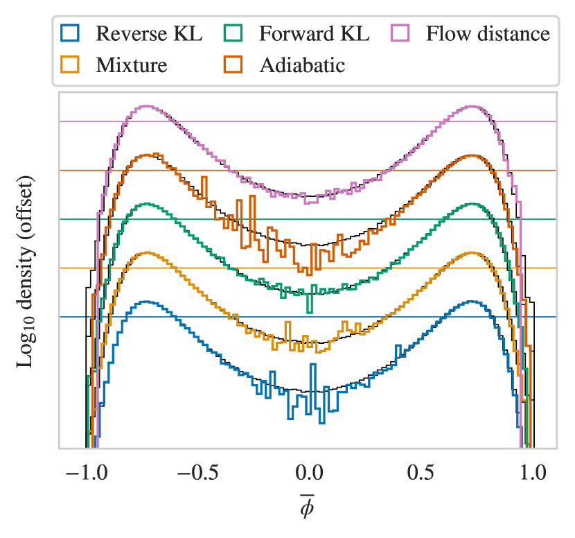
Figure 19: Distribution of $\overline{\phi}$ for ensembles generated using flow-based MCMC with models constructed using the different approaches described in the text, all for $m^{2}=-4$ and $\alpha=0$. The log distributions are offset for clarity; the horizontal line of the same color indicates density 1 for the corresponding distribution, and lines are separated by factors of 10. The true distribution of $\overline{\phi}$, estimated using AHMC, is shown in black behind each curve.

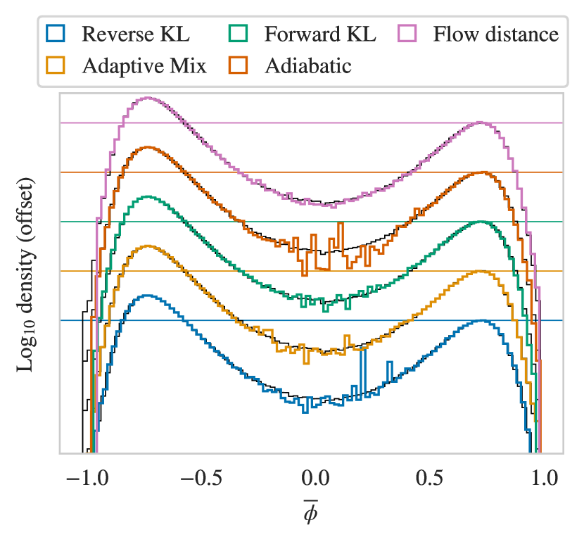
Figure 20: As in Fig. 19, but for $m^{2}=-4$ and $\alpha=0.8/V$.

Figure 21 shows the results of using the various different models with flow-based MCMC to compute the observables $\langle\overline{\phi}\rangle_{p}$ and $\langle\overline{\phi^{2}}\rangle_{p}$, compared against “ground truth” computed using AHMC. We apply Independence Metropolis to a sample of $10^{6}$ configurations drawn from each model to generate an ensemble of target-distributed configurations. For both HMC samples and flow samples, we first bin the data to remove autocorrelations then bootstrap to estimate uncertainties. Most observables computed using flow-based MCMC agree within errors with the AHMC results (or the analytic value $\langle\overline{\phi}\rangle=0$ when $\alpha=0$) and no systematic bias is apparent.

However, a few points in Fig. 21 lie many standard deviations away from the true values, indicating their errors are severely underestimated. Additionally, we observe a larger-than-expected range of estimated errors given the apparently comparable quality of these models as measured by the forwards KL divergence and acceptance rate. We also obtain significantly different error estimates when analyzing different samples of $10^{6}$ configurations drawn from the same model, indicating non-convergence of variance estimates even for these large sample sizes. We trace these effects to the presence or absence in each sample set of high-weight configurations which trigger long rejection streaks. This implies that the Markov chains have not entered the smoothly converging regime even at length $10^{6}$, and thus that flow-based MCMC converges pathologically slowly when used with these models.

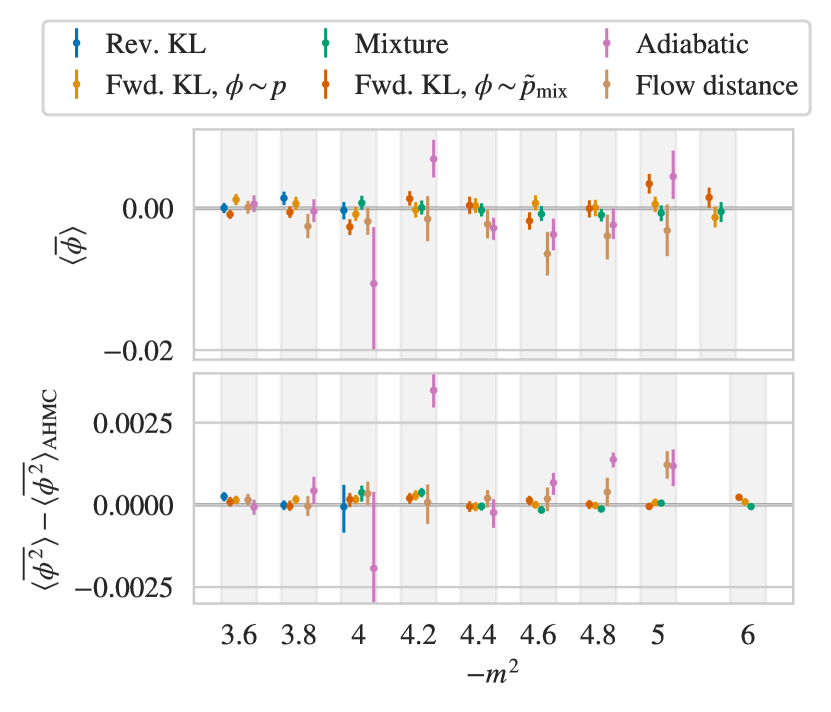
(a)

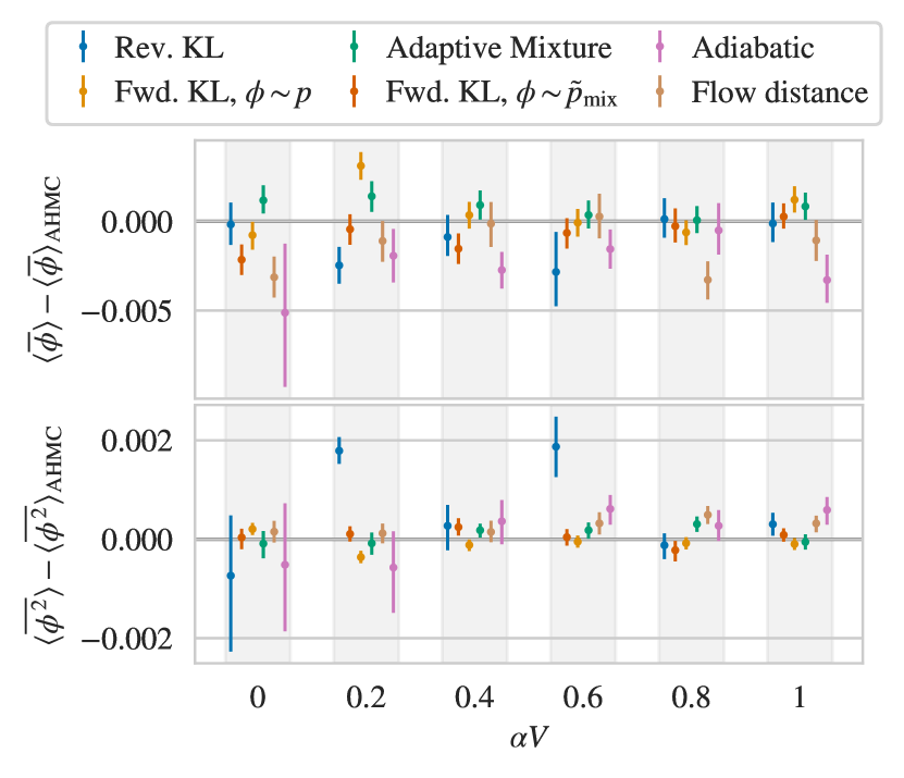
(b)

​

Figure 21: Estimates of $\langle\overline{\phi}\rangle$ and $\langle\overline{\phi^{2}}\rangle$, computed with flow-based MCMC using models obtained using the different approaches described in the text, for LABEL:sub@fig:cf_obs_M2 fixed $\alpha=0$ varying $m^{2}$ and LABEL:sub@fig:cf_obs_alpha fixed $m^{2}=-4$ varying $\alpha$. Observables are computed by drawing $10^{6}$ configs from each model, applying independence Metropolis to construct a Markov chain, binning by $10^{4}$, and bootstrapping to estimate the error. Markers denote the median over bootstraps, and error bars extend to the 15.9th ($-1\sigma$) and 89.1th ($+1\sigma$) percentiles. Except for $\langle\overline{\phi}\rangle$ when $\alpha=0$, which is zero by symmetry, ground-truth values computed on ensembles of $10^{6}$ samples generated with AHMC have been subtracted from each observable, without accounting for the error in the AHMC estimate. Estimates that are consistent with zero within error indicate agreement with ground truth. Additional variance due to seed dependence in training and sampling is not quantified.

We also consider the reweighting-motivated effective sample size (ESS) per configuration, defined as

$$\text{ESS}/N\equiv\frac{1}{\int d\phi~{}\tilde{p}(\phi)w(\phi)^{2}}\approx\frac{1}{N}\frac{\left(\sum_{i}w_{i}\right)^{2}}{\sum_{i}w_{i}^{2}}$$ (30)

where the integral is the asymptotic value, in which sample dependence necessarily disappears and the metric reflects a property of the model, and the finite-sample estimator is evaluated for a sample of $N$ model-distributed configurations ${\phi_{i}\sim\tilde{p}}$ where $w_{i}=w(\phi_{i})=p(\phi_{i})/\tilde{p}(\phi_{i})$ as defined in Eqn. (23). The ESS per configuration falls between 0 and 1, achieving the maximum value of 1 for a perfect model $\tilde{p}=p$ where all $w_{i}=1$. The ESS is known to be (positively) biased for small sample sizes Elvira et al. (2018) so, in principle, it is important to sample until the estimator converges to obtain a meaningful metric of model quality. However, we observe large variances of ESS estimates even when computed from samples of $10^{6}$ configurations and, drawing different samples from the same models, we observe significantly different estimates, again indicating non-convergence. We trace this effect to the same high-weight configurations that break convergence of error estimations; we observe individual configurations that change the ESS by $O(1)$ factors, as discussed further in the next subsection.

To circumvent finite-sample limitations, we use a target-sample estimator of the asymptotic ESS per configuration,

$$\text{(ESS)}/N =\frac{1}{\int d\phi~{}p(\phi)\frac{\tilde{p}(\phi)}{p(\phi)}w(\phi)^{2}}$$ (31)

$$=\frac{1}{\int d\phi~{}p(\phi)w(\phi)}\approx\frac{N^{2}}{\left(\sum_{i}w_{i}\right)\left(\sum_{i}\frac{1}{w_{i}}\right)}\;,$$

where $\phi_{i}\sim p$ and the estimator incorporates the stochastic estimator of Eqn. (22) to allow use with unnormalized reweighting factors. The resulting ESS estimates for the different models are shown in Fig. 22, measured using the same shared ensembles of $10^{6}$ configurations of target-distributed samples used for the forwards KL divergence estimates in the previous section. We observe that $\text{ESS}/N\approx 0$ for most of the models. This should not be read as a deficiency of the ESS as a metric, but rather as a direct indication that these models will give poor-quality results when used with reweighting or direct resampling; as motivated further below, this also diagnoses the unsuitability of these models for use with flow-based MCMC.

The high variance in some of these target-sample ESS estimates, as well as the analysis in the next subsection, suggests that some or all of these estimates may still be poorly converged. However, some features of Fig. 22 merit discussion. We see $\text{ESS}/N\approx 0$ for all models with $m^{2}<-4.4$; the large errors on some models reflect cases where only a few high-weight samples cause the ESS to be small, similar to what is observed using the model-sample estimator. In many cases, forwards KL training with AHMC data is able to produce models with nonzero ESS where the other schemes cannot. A few models trained using other procedures have nontrivial ESS, but there is no pattern to this apparent success, and this could be due to the particular target samples used for these estimates. In a few spot checks, we observe strong seed dependence; for example, in Fig. 22a the model trained with AHMC data for $m^{2}=-4.2$ has nontrivial ESS but, as discussed further below, the model studied in the next section (trained similarly, for the same parameters) has $\text{ESS}\approx 0$.

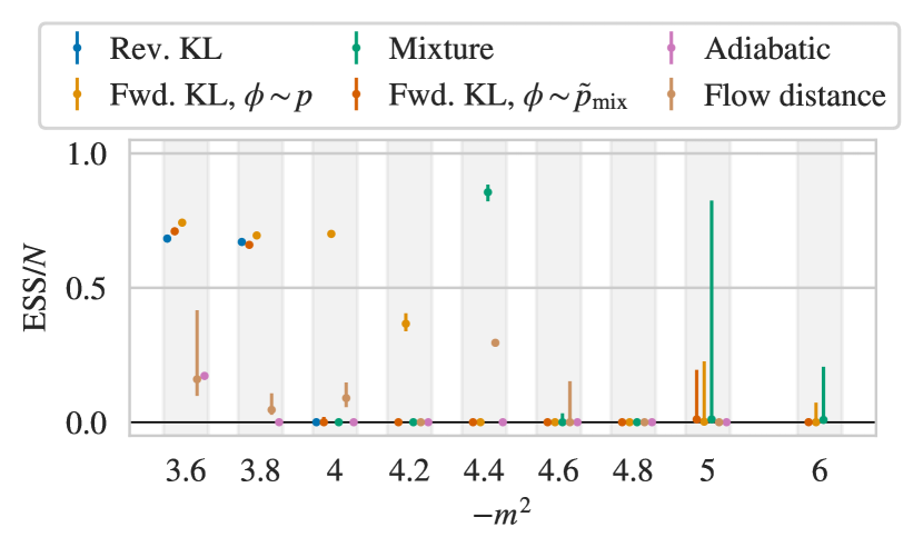
(a)

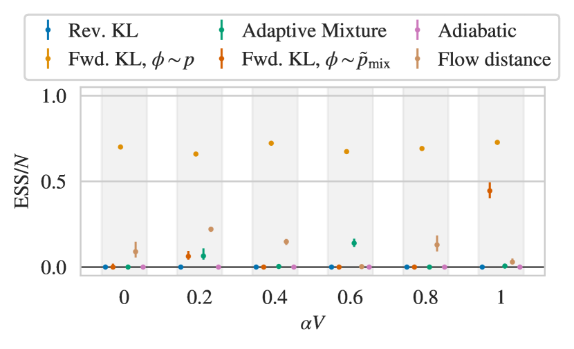
(b)

​

Figure 22: ESS per configuration estimated using target-distributed samples for models constructed using the different approaches described in the text, for LABEL:sub@fig:cf_ess_M2 fixed $\alpha=0$ and varying $m^{2}$ and LABEL:sub@fig:cf_ess_alpha fixed $m^{2}=-4$ and varying $\alpha$. All estimates are made on shared ensembles of $10^{6}$ samples, and errors are computed by bootstrapping. Markers denote the median over bootstraps, and error bars extend to the 15.9th ($-1\sigma$) and 89.1th ($+1\sigma$) percentiles. Additional variance due to seed dependence in training and sampling is not quantified.

VII.2 Case study: flow-based MCMC

To better understand the apparent convergence problems observed in the previous section, we perform a careful study of one particular model. We find that it exhibits exactly the issue discussed in Sec. II, where a rarely sampled-from region of configuration space is also highly underweighted in the model relative to the target, leading to pathologically slow convergence.

The model in question was trained targeting ${m^{2}=-4.2}$ and $\alpha=0$ with forwards KL training using AHMC samples; we chose a model trained with this scheme as it produces the best bimodal models, so any issues observed apply for best-case training. The model discussed here is different than the one presented in Fig. 22a, but trained identically up to the random seed. Unlike for that model, we measure $\text{ESS}\approx 0$ using the target-sample estimator; meanwhile, the forwards KL divergence and MCMC acceptance rate are lower outside error for the present model, but closely comparable in magnitude. This indicates that different initial weights and different sets of training data can yield models with drastically reduced ESS without qualitatively affecting the forwards KL divergence or MCMC acceptance rate. As explored below, this low observed value of the ESS signals severe problems with flow-based MCMC using this model which are not diagnosed by the other two metrics.

For all numerics in this section, we use a single dataset of $10^{6}$ model-distributed samples drawn from the flow model and another set of $1.28\times 10^{6}$ target-distributed samples generated with AHMC. We normalize all reweighting factors $w(\phi)=p(\phi)/\tilde{p}(\phi)$ such that $\langle w\rangle_{\tilde{p}}=1$ using the stochastic $Z$ estimator of Eqn. (22) evaluated on the target samples. Most of the ensuing discussion is phrased in terms of the distribution of reweighting factors under the model,

$$\tilde{\rho}(w) \equiv\left\langle\delta\left(w-\frac{p(\phi)}{\tilde{p}(\phi)}\right)\right\rangle_{\tilde{p}}=\int d\phi~{}\tilde{p}(\phi)\delta\left(w-\frac{p(\phi)}{\tilde{p}(\phi)}\right)\,.$$ (32)

which contains all observable-independent information about model quality. Although correlations between reweighting factors and observables can further affect the quality of specific measurements, we are interested in model quality generically.

Figure 23 demonstrates that the large variation in the ESS estimates derived from different model sample datasets, as well as the low values of the ESS estimated using target samples, are due to configurations from the high-weight tail of the distribution of reweighting factors. The two sets of points in the figure correspond to the estimate of the ESS (corresponding to reweighting from model to target) including all samples with $w\leq w_{\text{max}}$, varying $w_{\text{max}}$. Considering the model-sample estimator in isolation, as the cut $w_{\text{max}}$ is increased, the ESS appears to be converging to a value $\sim 0.7$ until two high-weight “outlier” configurations significantly reduce it; the highest-weight configuration reduces the ESS by a factor $\sim 2$. Comparison with the target-sample estimator indicates that these apparent outlier configurations correspond to an unsampled high-weight tail of configurations. The discrepancy between the highest-weight model-estimator point and the target-sample curve can be attributed simply to coarse sampling in the tail. The target-sample estimator smoothly approaches a near-zero value, although undersampling in the tail suggests the exact value estimated is unreliable, with $\sim 5$ samples accounting for the difference between $0.15$ and $\approx 0$.

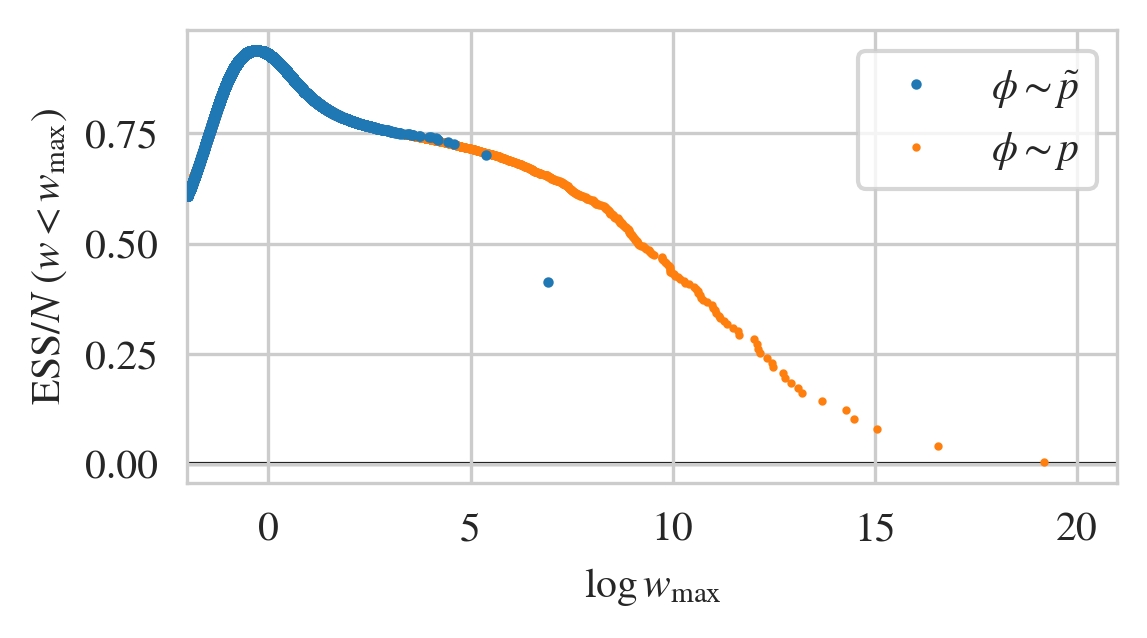
Figure 23: Running value of the ESS per configuration (for reweighting from the model to target) computed including the subset of configurations with $w<w_{\mathrm{max}}$, using either model (blue) or target (orange) samples and the corresponding estimators as described in the text.

Figure 24 confirms directly the existence of an undersampled high-weight tail in the distribution of reweighting factors. The histogram in blue corresponds to the distribution of reweighting factors estimated directly using model-distributed samples. The distribution of reweighting factors under the model can also be obtained by reweighting the distribution of reweighting factors under the target ${\rho(w)=\langle\delta(w-p/\tilde{p})\rangle_{p}}$,

$$\tilde{\rho}(w) =\int d\phi~{}p(\phi)\frac{\tilde{p}(\phi)}{p(\phi)}\delta\left(w-\frac{p(\phi)}{\tilde{p}(\phi)}\right)=\rho(w)/w$$ (33)

which we apply to a histogram estimate of $\rho(w)$ made with target-distributed samples to produce the histogram in orange. In Fig. 24, the reweighted histogram satisfies $\int dw~{}\rho(w)\approx 1$, and matches well with the direct estimate where the two both have support; however, it also reveals a long tail of high-weight configurations which are not sampled in $10^{6}$ draws from the model.

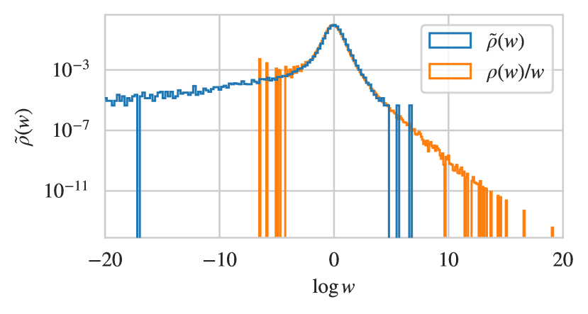
Figure 24: The distribution of reweighting factors under the model, $\tilde{\rho}=\langle\delta(w-p/\tilde{p})\rangle_{\tilde{p}}$, with the blue histogram made using $10^{6}$ model-distributed samples and orange histogram made using $1.28\times 10^{6}$ target-distributed samples generated with AHMC then reweighted. The two isolated “outlier” points from Fig. 23 are visible at large $w$ in the blue histogram.

Identifying the tail as all samples with $w>5$ (corresponding roughly to the first outlier in Fig. 23 and Fig. 24), Figure 25 examines where these high-weight configurations lie with respect to the distributions of other observables under the target. The high-weight tail comes from regions of very low density in the model, accounting for their infrequent sampling. As suggested by the rejection-induced finite-sample fluctuations near $\overline{\phi}\approx 0$ in Figs. 19 and 20, the high-weight configurations come from the inner tails of the bimodal distribution. This corresponds to samples from the lower-valued tail of the distribution of $\overline{\phi^{2}}$, explaining the more severe effect on the variance of this observable in Fig. 21, and between different model-generated samples as discussed above, compared with $\overline{\phi}$ where duplications due to rejections enter near the midpoint of a symmetric distribution.

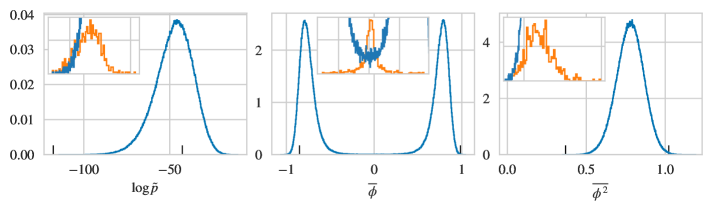
Figure 25: Distributions of $\log\tilde{p}$, $\overline{\phi}$, and $\overline{\phi^{2}}$ under the target $p$. The blue lines include all data, while the orange lines show the undersampled tail and include only configurations with $w>5$, corresponding roughly to where the model distribution (with $10^{6}$ samples) cuts off in Fig. 24 and where the two “outlier” points sit in Fig. 23. The additional spines on the x axes indicate the extent of the insets.

Due to its undersampling, we cannot tractably study the effect of the high-weight tail by directly sampling using flow-based MCMC. Instead, we can use target-distributed samples to estimate the asymptotic properties of flow-based MCMC by considering the asymptotic behavior of the Markov process that defines it. After equilibration, the current configuration of any Markov chain generated using flow-based MCMC is target-distributed, and proposed updates are independent model-distributed configurations. Proposals are accepted with probability

$$A(\phi\rightarrow\phi^{\prime})\equiv\min\left(1,\frac{w(\phi^{\prime})}{w(\phi)}\right)\equiv A(w\rightarrow w^{\prime})$$ (34)

so the asymptotic acceptance rate is

$$A\equiv A(p\rightarrow\tilde{p}) =\int d\phi d\phi^{\prime}~{}p(\phi)A(\phi\rightarrow\phi^{\prime})\tilde{p}(\phi^{\prime})$$ (35)

$$=\int dwdw^{\prime}~{}\rho(w)A(w\rightarrow w^{\prime})\tilde{\rho}(w^{\prime})$$

where in the second line we use that the acceptance rate is a function of $w$ and $w^{\prime}$ only to rewrite the expression in terms of the distributions of reweighting factors. Evaluating this expression using target samples for the expectation over $p$, and model samples for the expectation over $\tilde{p}$, we find estimates consistent with the acceptance rates obtained by directly sampling using flow-based MCMC, as expected given that the high-weight tails comprise a small fraction of the mass of $p$.

We can extend this reasoning to estimate the asymptotic distribution of rejection runs and thus the autocorrelation time. We relegate the derivation to Appendix A, and summarize the results here: in terms of the “acceptance rate out of a configuration” with weight $w$,

$$A(w\rightarrow\tilde{p})=\int dw^{\prime}A(w\rightarrow w^{\prime})\tilde{\rho}(w^{\prime})$$ (36)

the asymptotic acceptance rate is

$$A(p\rightarrow\tilde{p})=\int dw\rho(w)A(w\rightarrow\tilde{p})$$ (37)

and the length $r$ of the rejection run following the initial acceptance of a configuration with weight $w$ is (geometrically) distributed as

$$p(r|w)=A(w\rightarrow\tilde{p})\left[1-A(w\rightarrow\tilde{p})\right]^{r}$$ (38)

from which we can derive the expected rejection length under the target

$$\langle R\rangle_{p}=\int dw~{}\rho(w)\frac{1-A(w\rightarrow\tilde{p})}{A(w\rightarrow\tilde{p})}$$ (39)

which is directly and trivially related to the rejection-run estimator Albergo et al. (2019) for the integrated autocorrelation time as

$$\tau_{\mathrm{int}}=\frac{1}{2}+\langle R\rangle_{p}.$$ (40)

Applying these expressions in Fig. 26, we find immediately that the asymptotic autocorrelation time either diverges or is too long to estimate even using target samples. Using model samples to estimate $A(w\rightarrow\tilde{p})$ as a function of $w$ and applying them to a histogram estimate of $\rho(w)$, we see that the integrand of the asymptotic acceptance rate has little mass present in the tail beyond $w\sim 5$, as expected given the consistent direct and asymptotic estimates of the acceptance rate. However, the integrand of the integrated autocorrelation time grows as $w$ increases, and because the variables of the theory are not compact, there is in principle no upper bound on the maximum $w$. Due to this lack of an upper bound we cannot conclude that the autocorrelation time diverges, as it is possible that the integrand turns over at even higher $w$; however, even if this is the case, the sampler is clearly pathological. By comparison, the autocorrelation time measured on ensembles generated using flow-based MCMC with this model is only $O(1)$, even on datasets of $O(10^{6})$ samples.

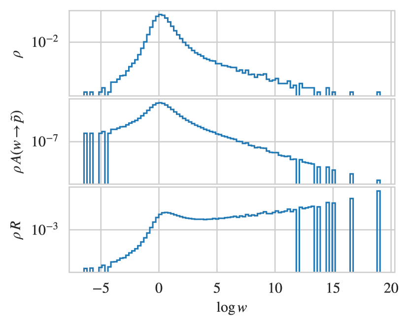
Figure 26: Top panel: distribution of reweighting factors under the target, $\rho(w)=\langle\delta(w-p/q)\rangle_{p}$, estimated using $1.28\times 10^{6}$ samples generated using AHMC. Bottom panels: integrands constructed from the distribution of reweighting factors as described in the text. Integrating over the second panel will yield the asymptotic acceptance rate, while integrating over the third panel gives the integrated autocorrelation time up to an offset of $+1/2$ as described in the text.

VII.3 Discussion: performance metrics for flow-based MCMC

The failure of the forwards KL divergence and MCMC acceptance rate to diagnose the pathology explored in the previous subsection indicates that they are unsuitable metrics of the quality of models for use with flow-based MCMC. These metrics fail because the problems with flow-based MCMC are caused by poor modeling in low-density regions. The forwards KL divergence, $\int d\phi~{}p(\phi)\log w(\phi)$, is insensitive to these regions: the weight $p$ is small therein, and the logarithm damps the effect of large $w$. The acceptance rate provides only a lower bound on the autocorrelation time Albergo et al. (2019), and this bound is particularly weak when the sampler may undergo long runs of rejections, as observed here. To illustrate: a Markov chain in which every other proposal is accepted has a much shorter autocorrelation time than one where half of the samples are replicates due to a single long rejection run, even though both chains have a 50% acceptance rate. The acceptance rate also fails to qualitatively penalize mode-collapsed models: for a symmetric bimodal system, the finite-sample acceptance rate will tend to be overestimated only by a factor of 2 versus the asymptotic one, as the rejections that populate the missed mode can only make up half of the total samples. A low divergence and high acceptance rate are necessary, but insufficient.

The ESS is more useful for this purpose, but must be interpreted carefully when evaluated using model-distributed samples in direct studies. Unlike the other metrics, the ESS penalizes models with broad distributions of reweighting factors that, as discussed above, lead to long MCMC autocorrelation times: high-weight configurations contribute more to the sum in the denominator of Eqn. (30) than the one in the numerator, while low-weight configurations contribute little to either but decrease the ESS via the $1/N$ factor. Similar arguments apply for Eqn. (31). The ESS also distinguishes mode-collapsed models from non-pathological ones, as the denominator clearly becomes large when $w(\phi)\gg 1$ over some mode of the target. In practice, the ESS is a more useful metric, especially when measured with target-distributed validation data; we found that high variance in the ESS estimated with model samples indicated low asymptotic ESS as estimated with target samples, and that this indicated problems with the models for use with flow-based MCMC. Low observed values of the ESS should be taken seriously, even if the MCMC acceptance rate is high.

VII.4 Case study: mixing flow-based MCMC and HMC

As motivated in Sec. III, composing different MCMC updates can produce samplers with better properties than either type of update alone. Specifically, we consider a Markov chain constructed by alternating $n_{F}$ flow-based MCMC updates with $n_{H}$ trajectories of HMC. Each type of update is applied completely independently and ends in its own Metropolis test, so neither algorithm needs any modification to use the two in combination.

In this scheme, the limit $n_{H}\gg n_{F}$ corresponds to augmented HMC as discussed in Sec. VI.2, except the augmentation step is a learned flow-based MCMC proposal rather than some mode-hopping transformation constructed by hand. As long as the flow model samples from all modes and has a nontrivial acceptance rate, this augmentation solves the problem of freezing in HMC. While this is not useful when simpler mode-hopping transformations are known, it may be possible to train multimodal flow models in the more general case (using e.g. flow-distance regularization) to provide machine-learned augmentation steps. However, in this case mixing of the Markov chain is primarily driven by HMC, and any critical slowing down beyond freezing will not be alleviated.

More interestingly, we can consider the regime where ${n_{F}>n_{H}=1}$, i.e. flow-based MCMC augmented with occasional applications of HMC. In the last section we saw that the asymptotic performance of purely flow-based updating with these models is compromised by long rejection runs triggered when high-weight configurations are accepted. Mixing in occasional HMC updates must solve this problem, as long rejection streaks will be terminated after enough HMC steps occur to move the chain to a better-modeled part of configuration space. The practical question to answer is thus how many HMC updates must be applied with what frequency to regulate the long rejection runs. Figure 27 demonstrates that (for the HMC parameters we consider in this paper) even a single HMC step moves the bulk of the tail samples with $w\gtrsim 5$ to smaller reweighting factors.

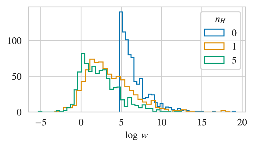
Figure 27: Effect of different numbers of HMC steps $n_{H}$ on a distribution of 800 samples from the underweighted tail with $w\gtrsim 5$. Histograms for $n_{H}\neq 0$ include a marginalization over 100 different HMC chains out of each configuration.

Asymptotic analysis of the behavior of the composite algorithm is complicated by the need to marginalize over all possible momentum draws as well as HMC’s dependence on the previous configuration, which means that the distribution of reweighting factors no longer captures all information about overall sampling performance. However, we can make estimates by considering the asymptotics of flow proposals made on top of fixed HMC evolutions. Between HMC steps, proposals are made completely independently to update a fixed configuration. We can model the distribution of rejection run lengths under the composite algorithm, starting from some initial configuration $\phi_{0}$, as a generalization of the geometric distribution

$$p(r|\phi_{0},\bm{\Pi})=\frac{\prod_{t\leq r}(1-A(t))}{\sum_{r^{\prime}}\prod_{t\leq r^{\prime}}(1-A(t))}$$ (41)

where $A(t)$ is a time-dependent acceptance rate out of the configuration. Before the first HMC step, ${A(t)=A(\phi_{0}\rightarrow\tilde{p})}$ as in the pure-flow case; after the first HMC step, $A(t)=A(\phi_{1}\rightarrow\tilde{p})$ where $\phi_{1}$ is the evolved configuration. We have made explicit the dependence on the (infinite) set of momentum fields $\bm{\Pi}$ drawn for use in all ensuing HMC steps, which must be marginalized over to quantify asymptotic sampling performance. In practice we compute this distribution for a fixed HMC chain beginning with $\phi_{0}$, and marginalize by including estimates made using 100 different chains with different seeds. After 100 trajectories the unnormalized geometric distributions are zero within numerical precision, even for $n_{F}=1$, indicating that expectations computed using the truncated distributions are converged and accurate.

The results, shown in Fig. 28, demonstrate that even infrequent HMC steps will truncate long rejection runs. In the purely flow-based MCMC limit $n_{F}=\infty$, the typical run length following the tail samples is $\sim 10^{3}$, but the longest is $\sim 10^{8}$. A single HMC step per thousand flow steps, $n_{F}=1000$, does not change the typical run length appreciably, but does truncate the maximum run length to $\sim 10^{4}$, indicating that the neighborhoods of high-weight configurations are not extensive (as would be the case with a mode-collapsed model). As the frequency of HMC steps increases, the maximum escape time out of the tail configurations decreases progressively, and the shape of the distribution changes more substantially.

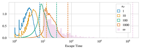
Figure 28: Distribution of expected number of rejections following configurations from the undersampled tail with $w\gtrsim 5$, for a Markov chain evolved by alternating $n_{F}$ flow-based MCMC proposals with single HMC trajectories. The escape time metric counts either a flow proposal or an HMC trajectory as one step. The distribution corresponds to $\sum_{r}rp(r|\phi)$, where $p(r|\phi)$ is as in Eqn. 41, computed as described in the text for 800 different tail samples $\phi$, and marginalized over 100 different HMC chains run out of each sample and over all different delays before the first HMC step occurs (i.e. after $0\ldots n_{F}$ flow proposals, with even weight). Each dashed vertical line indicates the largest value for the distribution shown in the same color.

The HMC updates must move configurations into the undersampled regions of configuration space to compensate for the truncation of the rejection runs that would have otherwise populated them. However, as shown in Fig. 29, while the HMC augmentation introduces high-weight configurations more frequently in a relative sense, this happens only infrequently in an absolute sense. Using our target-distributed ensemble of $1.28\times 10^{6}$ configurations, we estimate that only $\sim 0.05\%$ of the mass of $p$ is in the high-weight tail where $w>5$. We apply 1000 HMC updates to each of these configurations, generating an ensemble of Markov chains. Updating one target-distributed ensemble with HMC yields another, but will move some fraction of the original ensemble into the tail and some fraction out. We find that each HMC update moves $\sim.03\%$ of $p$ into the tail, which corresponds roughly to the probability that an HMC augmentation step will introduce a high-weight configuration. Subsequent updates rapidly move these configurations back out of the tail, as shown in Fig. 29 and similarly demonstrated in Fig. 28.

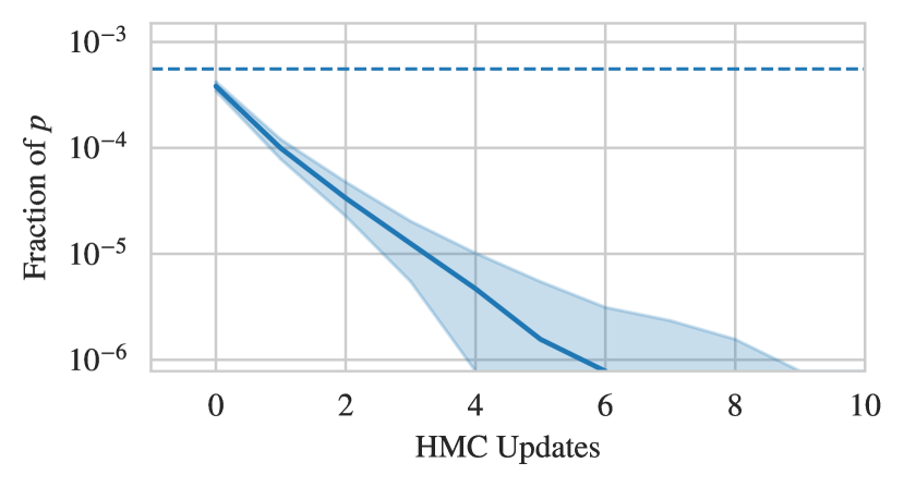
Figure 29: Time for HMC updates to move out of the high-weight tail (where $w>5$) after first entering it, computed as described in the text. The dashed line indicates the fraction of $p$ in the high-weight tail, $\sim 0.05\%$. At zero HMC steps, the value indicates the fraction of $p$ which one HMC update newly moves into the high weight tail, $\sim.03\%$, which decays as HMC moves these configurations back out of the tail. The solid line denotes the median fraction, while the band spans the 1st to 99th percentiles.

These results demonstrate that augmenting flow-based MCMC with occasional HMC updates regulate the issues arising in flow-based MCMC, providing a sampler with all the advantages of independence Metropolis without the risk of slow convergence. This yields a qualitative advantage over traditional algorithms in cases where freezing occurs. A more quantitative comparison of the relative performance of HMC and the composite algorithm is application-dependent and beyond the scope of this exploratory study. The performance of the composite algorithm depends not only on the model, but also on the tuning of the HMC augmentation step, whose optimal parameters depend on the structure of the lattice theory as well as the model being augmented.

VIII Extensions & other approaches

VIII.1 Constructing multimodal models

In this work we demonstrate basic applications of the methods described in Secs. IV and V to training bimodal models for real scalar $\phi^{4}$ theory in two dimensions. The results of this study suggest some obvious extensions, listed below.

Adiabatic retraining and flow-distance regularization may each be used in combination with forwards KL self-training, rather than with reverse KL self-training. More generally, each of these procedures may be considered as a deformation of the target, and so may be used with any training procedure.

Flow-distance regularization and (to a lesser extent) adiabatic retraining require careful design of a schedule to avoid mode collapse. Schedulers designed to detect and prevent mode-collapse can make these methods more practical to apply, but require an investigation of metrics to anticipate mode collapse during training.

As demonstrated in Sec. VI.3.3, forwards KL self-training can be made to work with a naive data augmentation scheme instead of the more-principled approach of generating training data using a mixture model. Naive data augmentation could allow application of forwards KL self-training to learning distributions with extended modes that arise due to spontaneous breaking of a continuous symmetry, as symmetrized mixture model densities are intractable to evaluate in this case. The alternative, training with mixtures symmetrized over discrete approximations of the group, does not encode the full symmetry in the data and scales poorly with the group dimension.

Self-training with the reweighted forwards KL divergence is generically more expensive than reverse KL self-training, and especially so when training samples are drawn from a mixture. However, we observed that bimodal models are typically stable against mode collapse under reverse KL self-training. This suggests using forwards KL self-training only early in training, switching to reverse KL after circumventing the regime where mode collapse may occur.

The forwards KL self-training scheme presented in this paper allows for data augmentation in combination with self-training generically, which may have useful applications other than putting in mode structures by hand.

This study considered only the reverse KL and forwards KL divergences (and simple generalizations thereof) as losses. As noted in Ref. Wu et al. (2021), the reverse KL divergence is an integral over $\tilde{p}\log\tilde{p}/p$, so the loss is only sensitive to large discrepancies between $\tilde{p}$ and $p$ when $\tilde{p}$ is not small. A similar argument with $\tilde{p}\rightarrow p$ applies for using the forwards KL divergence as a loss. At finite sample sizes, this problem manifests as poorly resolved contributions to the gradients from rarely sampled regions, making it difficult for any training scheme using KL divergences as losses to achieve accurate modeling of those regions. As discussed in Sec. VII.2 (see Fig. 25), problematic high-weight configurations arise from mismodeling in exactly these low-density regions. Further, as noted by Ref. Del Debbio et al. (2021), the mode-seeking effect of reverse KL self-training tends to produce models which undersample from the tails of distributions. Training with different losses may be able to produce models with better-behaved distributions of reweighting factors. Similarly, it may be possible to use self-training schemes which produce additional samples from underweighted regions (as data augmentation with the forwards KL self-training procedure does for the different modes in this work).

Mixtures are a common prescription for smoothing out pathological reweighting factor distributions Owen (2013). In this work we constructed symmetrized mixtures over the global $Z_{2}$ symmetry of the target, which is not a symmetry of our model architecture. We considered only mixtures constructed with mode-collapsed unimodal flow models, but the resulting models compared well with truly bimodal flow models, and our results suggested some of these mixtures had nontrivial ESS where bimodal flow models failed. Applying the symmetrized mixture construction to bimodal flow models trained using the other methods may help regulate the distribution of reweighting factors and provide models that can be used with flow-based MCMC. There are additional symmetries that could be exploited in this manner, like the $Z_{2}$ subgroup of translational symmetries broken by the checkerboard masking used in our coupling layers.

The methods described here are based on training a general flow model, but one can also consider using architectures specialized to learning a particular mode structure. Although not possible for general multimodal distributions, in the special case where a spontaneously broken global symmetry gives rise to the multimodal structure, symmetry-invariant models constructed using equivariant flows identically model all modes and thus are not susceptible to mode collapse. To this end, Ref. Nicoli et al. (2020b) used $Z_{2}$-equivariant flows and Ref. Del Debbio et al. (2021) used nearly-invariant flows to successfully model the multimodal phase of the same theory considered here. Further investigation is warranted, especially for the case of targets with extended modes.

Affine architectures have been shown to produce poor representations of bimodal distributions when used with unimodal priors Wu et al. (2020), an effect related to the flow’s inability to change the topology of the prior distribution Cornish et al. (2020). Thus, flow models built upon multimodal priors may provide better performance.

VIII.2 Flow-based sampling & inference

In this work we considered the performance of flow-based MCMC, reweighting, and the composite flow/HMC sampling algorithm. However, these are only a few means of inferring properties of the target distribution using flow models, and the broader class of flow-based approaches to sampling and inference remains yet to be explored. We list some interesting options below.

Ref. Wu et al. (2021) encountered similar problems with high-weight configurations as seen in this study. Rather than augmenting flow-based MCMC steps with HMC, that work regulated the effect of high-weight configurations using augmented MCMC (as described in Sec. III) to propose updates by transformations which are symmetries of the target, but not the model, with the reasoning that all configurations in the symmetry orbit are unlikely to be high-weight. This method can be used in combination with or instead of the HMC augmentation used here, although it is unclear whether this approach would be as helpful for the translationally symmetric architectures considered in this work. This provides a less expensive alternative to constructing mixtures over the same symmetry groups, which require evaluation of the model for all configurations in the symmetry orbit, rather than possibly only a randomly chosen subset.

Defensive mixtures Hesterberg (1995) provide another means of incorporating target samples, wherein samples are drawn stochastically from either the model distribution or from the target (necessitating a separate reservoir of target-distributed samples generated with e.g. HMC). This approach directly clips the distribution of reweighting factors, imposing a maximum $w$ even for non-compact variables. Unfortunately, this construction requires evaluating the normalized normalized target density ${p=\exp[-S]/Z}$, which is not generally possible in the lattice field theory context. However, it may be possible to use flow-based stochastic estimators of $Z$ Nicoli et al. (2020b) to estimate $w$ for use with reweighting; further work is required to determine the conditions for exactness of this approach. It is unclear whether an approach based on stochastic $Z$ estimation can be reconciled with MCMC sampling algorithms like the pseudo-marginal method Andrieu et al. (2009).

Stochastic normalizing flows Wu et al. (2020) generalize fully deterministic coupling layers to stochastically sampled conditional distributions, while still admitting exact and tractable computation of importance weights. It may be possible to use this framework to incorporate updates with (or inspired by) traditional MCMC algorithms directly into the models, rather than using them to augment deterministic flow proposals as done in this work.

Validated variational inference Huggins et al. (2020) may provide an alternative to MCMC or reweighting, where error estimates from sampling statistics are augmented with systematic errors provided by formal bounds on discrepancies between expectations under different distributions. In this framework, these explicit error bounds may be directly related to distances between distributions and can be formally incorporated into the variational inference workflow. This can be achieved by using a distance measure that incorporates an underlying metric in the space of probability measures, e.g. integral probability metrics Müller (1997), or by bounding such a distance with a linear combination of scale invariant $\alpha$-divergences. The latter is achievable without considerable computational overhead beyond what is normally necessary in variational inference contexts.

It may be possible to improve upon reweighting using recent developments in stabilizing importance ratios, e.g. by fitting tails with generalized Pareto distributions Vehtari et al. (2021). Such approaches may also provide new diagnostics of model quality based on the reliability of the importance weight.

IX Conclusion

In this work, we present a set of methods for constructing and training flow models for multimodal distributions in lattice field theory, and demonstrated their application to the bimodal distributions that arise in the $Z_{2}$-broken phase of real scalar field theory. The different approaches each solve the problem of mode collapse; however, which method is most suitable necessarily depends on the particular target.

For example, mixture models and data-augmented forwards KL self-training are simple to use, but require significant a priori knowledge about the mode structure of the distribution of interest. Without a complete set of mode-hopping transformations, mixtures constructed out of a single flow model and forwards KL self-training as described here are inapplicable. Further, if the mode-mixing transformations are not approximate symmetries as they are in the numerical study of this work, these methods may not perform as well as observed here. Mixtures constructed out of multiple different flow models are applicable, but still require knowledge of the mode structure to guarantee coverage of all modes. These methods are useful for constructing samplers, but not useful for investigating unknown distributions.

In contrast, the adiabatic retraining and flow-distance regularization methods are more difficult to apply, involving devising and testing different training schedules. Unlike in the example considered here, mode structures cannot always be easily controlled by adjusting action parameters, so employing adiabatic retraining may require devising regulating operators to add to the action. However, in principle, these methods require no a priori knowledge of the mode structure, and it may be possible to use them to investigate unknown mode structures.

We find that the flow models obtained using our various methods can be used to construct efficient samplers when employed with a composite algorithm which interleaves occasional HMC updates into flow-based MCMC, although they are unsuitable for use as samplers with flow-based MCMC alone. The problems with flow-based MCMC caused by undersampled high-weight tails in these models are not obvious when directly sampling and required target-distributed validation data generated with augmented HMC to diagnose and an asymptotic analysis to understand. These problems are not identified by either the forwards KL divergence or the flow-based MCMC acceptance rate, which are insensitive to small undersampled regions. The ESS is sensitive to these regions, but their effect manifests indirectly in model-sample estimators. Further work on diagnostics and metrics of model quality for flow-based MCMC is necessary, especially ones that do not require target samples. Similarly, although we demonstrate that the composite sampling algorithm can solve the problems of flow-based MCMC with high-weight configurations, it is unclear how to (tractably) quantify the asymptotic performance of the resulting samplers. Further analysis of this algorithm, and ideally metrics of model quality specifically for this application of flow models, will be necessary.

It should be noted that the high-weight tails which exist in our models are not necessarily a generic feature of flow-based models. We identify two features of our study as likely exacerbators of this problem: non-compactness and affine architectures. Real scalar field theory has non-compact variables, and so the reweighting factors are unbounded; by contrast, theories with compact variables are guaranteed to have a maximum $w$, so high-weight tails are naturally regulated, and the possible divergence of the flow-based MCMC integrated autocorrelation time observed in Sec. VII.2 cannot occur. Since we observe undersampled high-weight tails nearly ubiquitously, for all the methods considered, it may also be the case that the (fixed) affine architecture we consider here may be insufficiently expressive to capture the bimodal distribution. The problem could be a consequence of the non-universality of individual affine coupling layers, which cannot produce multimodal conditional distributions in isolation Wehenkel and Louppe (2020).

In summary, the results presented in this work show that multimodal lattice field theory distributions are not an obstacle to flow-based methods. Simultaneously, this study demonstrates that not all flow-based approaches to inference are equivalent, and problems with one approach do not mean all others must fail. There is a broad class of methods to be explored, each with their own advantages, disadvantages, and scaling properties; it remains an open question which will be most useful for lattice field theory.

Appendix A Asymptotic analysis of flow-based MCMC autocorrelations

Because each proposal in a flow-based MCMC chain is completely independent of any previous proposal and of the current state of the chain, the acceptance rate given that the current configuration is $\phi_{i}$ (the “acceptance rate out of $\phi_{i}$”) is always

$$a_{i} \equiv a(\phi_{i})=A(\phi_{i}\rightarrow\tilde{p}) =\int d\phi^{\prime}~{}A(\phi_{i}\rightarrow\phi^{\prime})\tilde{p}(\phi^{\prime})$$ (42)

$$=a(w_{i})=A(w_{i}\rightarrow\tilde{p}) =\int dw^{\prime}~{}A(w_{i}\rightarrow w^{\prime})\tilde{\rho}(w^{\prime}).$$

This value is independent of how many updates have been proposed and can be thought of as a property of a configuration or, as emphasized in the second line, as a function of the weight of the current configuration $w_{i}$. In terms of this quantity, the global asymptotic acceptance rate is

$$A\equiv\int d\phi_{i}~{}p(\phi_{i})a(\phi_{i})=\int dw_{i}~{}\rho(w_{i})a(w_{i}).$$ (43)

Because each proposal is independent, the number of rejections following the initial acceptance of $\phi_{i}$ is geometrically distributed, i.e.

$$p_{i}(r)\equiv p(r|\phi_{i})=p(r|w_{i})=a_{i}\left[1-a_{i}\right]^{r}$$ (44)

where $r$ is the number of rejections before a new configuration is accepted (such that $r=0$ means the next proposal is accepted). The expected number of rejections following the initial acceptance of $\phi_{i}$ is thus

$$\begin{gathered}R_{i}\equiv R(\phi_{i})=R(w_{i})=\sum_{r}r~{}p_{i}(r)=\frac{1-a_{i}}{a_{i}}\\ \Leftrightarrow\frac{1}{1+R_{i}}=a_{i}\end{gathered}$$ (45)

such that the expected rejection run length under the target is

$$\langle R\rangle_{p} =\int d\phi~{}p(\phi)R(\phi)=\int dw~{}\rho(w)R(w)$$ (46)

$$\approx\frac{1}{N}\sum_{i}R_{i},\quad(\phi_{i}\sim p)\,.$$

Using the distributions of rejection runs following individual configurations $p(r|\phi)$, we can write an expression for the overall distribution of rejection runs $p(r)$ produced by flow-based MCMC:

$$p(r) =\int d\phi~{}\frac{p(\phi)}{1+R(\phi)}p(r|\phi)~{}\bigg{/}\int d\phi~{}\frac{p(\phi)}{1+R(\phi)}$$ (47)

$$=\frac{1}{A}\int d\phi~{}p(\phi)a(\phi)p(r|\phi)$$

$$=\frac{1}{A}\int dw~{}\rho(w)a(w)p(r|w)$$

$$\approx\frac{1}{A}\frac{1}{N}\sum_{i}a_{i}~{}p_{i}(r)\;,\quad(\phi_{i}\sim p)\,.$$

In the first line, the factor $1/(1+R(\phi))$ compensates for the difference in counting between $p(\phi)$, which encodes every appearance of $\phi$ including duplications due to rejections, versus the counting of rejection runs following each initial acceptance of $\phi$. The integral in the denominator of the first line normalizes $p(r)$ such that $\sum_{r}p(r)=1$, and in the second line we recognize using Eqn. (45) that this integral is simply the asymptotic acceptance rate $A$. Note that $\langle R\rangle_{p}$ is different from the average rejection run length, which can be computed straightforwardly from Eqn. (47) as $\sum_{r}rp(r)=(1-A)/A$.

We can write an asymptotic estimator for the rejection-run autocorrelation function $p_{t\text{rej}}=\rho(t)/\rho(0)=\mathrm{AC}(t)$ (defined in Ref. Albergo et al. (2019)) in terms of the above expression for $p(r)$,

$$\mathrm{AC}(t) =A\sum_{r\geq t}\sum_{r^{\prime}\geq r}p(r^{\prime})=A\sum_{r\geq t}(r-t+1)p(r)$$ (48)

$$=\frac{1}{N}\sum_{i}a_{i}\frac{(1-a_{i})^{t}}{a_{i}}=\frac{1}{N}\sum_{i}p_{i}(t)(1+R_{i})$$

where the factor of the acceptance rate $A$ fixes overcounting of rejection runs (for a sample of $N$ there are $AN$ newly accepted configurations, each of which is followed by $r\geq 0$ rejections), and we see in the second line that we recover the intuitive expression ${\mathrm{AC}(t)=\langle\left[1-A(\phi\rightarrow\tilde{p})\right]^{t}\rangle_{\phi\sim p}}$. From this we can compute the integrated autocorrelation time for the rejection-run estimator,

$$\tau_{\mathrm{int}} =\frac{1}{2}+\sum_{t=1}\mathrm{AC}(t)=-\frac{1}{2}+\sum_{t=0}\mathrm{AC}(t)$$ (49)

$$=-\frac{1}{2}+\frac{1}{N}\sum_{i}(1+R_{i})=\frac{1}{2}+\langle R\rangle_{p}$$

where we have used that $\sum_{t}p(t|\phi_{i})=1$. We see from Eqn. (49) that the integrated autocorrelation time is directly and trivially related to $\langle R\rangle_{p}$.