Modeling the Variable Polarization of $\epsilon$ Aurigae In and Out of Eclipse

Abstract

The eclipsing binary $\epsilon$ Aur is unique in being a very long-period binary involving an evolved, variable F star and a suspected B main-sequence star enshrouded in an opaque circumstellar disk. The geometrical arrangement is that the disk is viewed almost perfectly edge-on, with alignment leading to a partial eclipse of the F star. Despite a global observing campaign for the 2009-11 eclipse, there remain outstanding questions about the nature of the binary, its components, the disk, and the evolutionary state of the system. We analyze optical-band polarimetry in conjunction with broad-band color variations to interpret brightness variations across the surface of the F star. We model this both during and after the 1982-84 eclipse for which an extensive and dense data set exists. We develop a model in terms of surface temperature variations characterized by a small global variation overlaid with a temperature variation described with low-order spherical harmonics. While not providing a detailed fit to the dataset, our modeling captures the overall characterization of the color and polarimetric variability. In particular, we are able to recover the gross behavior of the polarimetric excursion in the Q-U plane as observed during eclipse of the F star when compared to post-eclipse behavior.

1 Introduction

The bright eclipsing binary system $\epsilon$ Aur (HD 31964) has the longest known orbital period (27.1 years) and longest duration primary eclipse ($\sim 2$ years) of all eclipsing binary stars. It is comprised of a large F0 star and a huge dark disk, most likely enshrouding an early B-type star, as the companion to the F star. Efforts to determine the nature of the nearly invisible disk-like companion have dominated observations of the system. However, information about the disk is obtained only by observations of its effects on light from the F star during the infrequent primary eclipses. The most recent 2009-2011 eclipse yielded a wealth of new results (Stencel, 2015, and references therein). In addition to increased photometric, spectroscopic, and spectropolarimetric monitoring, optical interferometric observations have led to synthetic images of the disk eclipsing the large F star on the sky (Kloppenborg et al., 2015).

There still remains a substantial uncertainty in the distance to the system though most recent works argue for a distance less than 1 kpc (Gibson et al., 2018). These latest observational constraints confirm $\epsilon$ Aur to be an interacting binary system. However, application of the latest stellar evolution codes for binary stars generates models that allow for the F star to range from a post-RGB type to a pre- or post-AGB type star (Gibson et al., 2018). The precise nature of the binary components of this system is still under debate.

As complex as the eclipsing disk surrounding a B-type star appears to be, interpretation of the eclipse observations remains a challenge as the F star is known to undergo semi-regular pulsations (Arellano Ferro, 1985; Kim, 2008; Ikonnikova et al., 2018). Spectro-interferometric observations of H$\alpha$ have also shown it to have an extensive P-Cygni like wind region (Mourard et al., 2012). The pre- and post-eclipse interferometric data of Kloppenborg et al. (2015) indicate the F star has a more-or-less constant diameter. However, they note some non-zero closure phases for their baseline models, coupled with variations in radius and limb darkening during eclipse, suggesting the possible presence of convective cells or thermal features (e.g., “spots”) on the surface. Such thermal variations may be expected to arise from non-radial pulsations (NRPs) and to produce a small linear polarization signature from a simple free electron scattering model (Stamford & Watson, 1980). Alternatively, the thermal variations could be represented by considering the stellar surface as radiating anisotropically with Thomson or Rayleigh single scattering in a spherical circumstellar envelope producing a polarization signature from components of the spherical harmonics of such anisotropy (Al-Malki et al., 1999).

Broadband polarization observations were made during the 1982-1984 eclipse (Kemp et al., 1986) and the 2009-2011 eclipse (Cole, 2012; Henson et al., 2012). A significant polarization signature is produced by the extreme asymmetry of the eclipse geometry. However, Henson (1989) proposed that NRPs of the F star create variable polarization with an amplitude similar to the effect of the eclipse and with a typical timescale on the order of 100 days. His work focused on the variability outside eclipse beyond the 1982-1984 event. Neither the Cole (2012) nor the Henson et al. (2012) observations were of the quality or density of those made by (Kemp et al., 1986) and Henson (1989). Cole (2012) did report variable polarization outside the eclipse similar in scale to that of Henson (1989), but his observations spanned only $\sim$150 days. Although Henson et al. (2012) observed several months pre-eclipse, the limited precision of the observations did not allow the detection of any significant variations outside of eclipse. As each of the above authors chose to analyze the eclipse behavior using $q$ and $u$ Stokes parameters with different coordinate reference frames (i.e., rotating the normalized parameters by different angles), a direct comparison of the eclipse polarization cannot be easily made (for an overview of Stokes parameters and polarimetry see e.g., Clarke, 2010). However, a simple qualitative comparison near the stages of egress (the only phase common to all observers) does show the polarization in both parameters changing significantly as the geometry of the system experiences its most dramatic change.

Broadband photometric variability is also present outside the eclipse. Persistent $\sim$0.1 magnitude variations exist on a timescale of $\sim$2 months, but both the amplitude and period vary unpredictably. This behavior, along with the elongated disk geometry, complicates the establishment of the contact points for the eclipse (Karlsson, 2012). In addition, Karlsson (2012) points out that ingress and egress have different lengths and slope variations. Thus, although the amplitude of the photometric variability outside eclipse is much smaller than the eclipse depth, its irregularity makes it harder to clearly define the features of the eclipse itself. For the polarization, it was noted earlier that the amplitude of the polarized light variations outside eclipse is significant when compared to the overall eclipse effect. Since they also vary unpredictably in amplitude and period, it is extremely difficult to separate eclipse effects from the behavior of the variable F star.

We construct here a simple model for a polarized atmosphere for the F0 star. A phenomenological model of surface brightness variations is introduced in an effort to characterize the aggregate properties observed in the variable polarization both in and out of eclipse for the star. In § 2, a review of the dataset used for comparison with the modeling is described. The description for our model of variable polarization is given in § 3. Results from the modeling are presented in § 4, with a summary of this study and concluding remarks given in § 5.

2 Observations

The $V$ band linear polarization measurements of $\epsilon$ Aur modeled here were obtained during and after the 1982-84 eclipse by Henson (1989). These comprise an extensive and precise set of measurements consisting of 969 nightly data points spanning from 1982 August to 1988 May (representing approximately 20 cycles of a generic pulsation period on the order of 100 days). The measurements were obtained using the photoelastic-modulator polarimeter attached to the 61 cm telescope at the University of Oregon’s Pine Mountain Observatory described in detail by Kemp & Barbour (1981). The dataset consists of instrumental $q$ and $u$ Stokes parameters given in percentage polarization with typical measurement errors of only 0.010% in the $q$ parameter and 0.015% in the $u$ parameter, with an instrumental polarization for the telescope/polarimeter system of less than 0.005%. Thus, these errors are an order of magnitude smaller than the typical 0.10% fluctuation from the mean $q$ and $u$ polarization values outside of eclipse.

In order to facilitate comparison to the model, the instrumental Stokes parameters were adjusted in two ways. First, a sizeable but constant interstellar component of $\sim 2\%$ is present for the measured polarization (Geise, 2015). Since the model would produce zero polarization for a symmetric geometry, the mean value established outside the eclipse was subtracted from each parameter. The remaining variability would thus be intrinsic to the pulsations of the F star. Second, as the binary system is seen edge-on to the orbital plane, the eclipse aspects of the model comparison can best be facilitated if the measured Stokes parameters are oriented relative to the orbital plane rather than presented as the standardized equatorial parameters which would align the $q$ parameter with north and south on the sky. We benefit from the interferometry results for the 2009-2011 eclipse (Kloppenborg et al., 2015) which establish a position angle of $297^{\circ}\pm 7^{\circ}$ on the sky for the disk-orbit plane. Thus, the original instrumental parameters were rotated with a Mueller matrix (which preserves the total polarization) by an angle of $-27^{\circ}$ to align the $q$ parameter perpendicular to the orbit plane. Figure 1 shows V band photometry from the AAVSO, the $q$ (red) and $u$ (blue) parameters, the percent polarization (black; $p=\sqrt{q^{2}+u^{2}}$), and the polarization position angle $\psi_{P}$ versus time for the rotated, normalized polarization measurements that we compare to the model results.

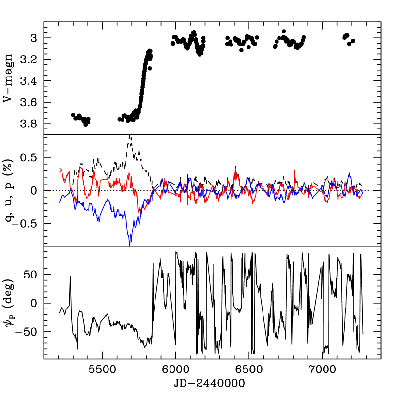
Figure 1: Shown are data from the 1980’s eclipse, with V magnitude at top, polarization amplitude at middle, and polarization position angle at bottom. The light curves are plotted against modified Julian date (JD) as indicated. For the middle panel, the dashed line is the total polarization $p$, red is $q$, and blue is $u$. All polarizations are indicated as percent.

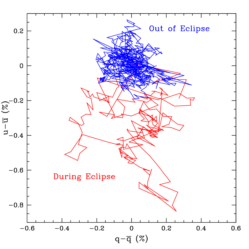
Figure 2: Here the $q$ and $u$ data from Fig. 1 are plotted in the $q-u$ plane. As labeled, the red portion is during eclipse, showing an excursion from the blue portion which is post-eclipse. The polarization is plotted relative to centroid values $\bar{q}$ and $\bar{u}$ associated with the post-eclipse data, assuming those average values represent the interstellar polarization and any stable intrinsic polarization to the binary system.

3 Model for Stellar Polarimetric Variability

3.1 Description of the Model

The intrinsic and variable polarization of the F star in $\epsilon$ Aur offers a number of challenges to modeling efforts. Owing to its low gravity, one needs to calculate polarized radiative transfer for a model atmosphere in spherical coordinates to account for extended atmosphere effects (Cassinelli & Hummer, 1971; Doherty, 1986; Kostogryz & Berdyugina, 2015; Kostogryz et al., 2016). Plus, the atmosphere must be time-dependent and 3-dimensional to capture fully and accurately the variable and asymmetric behavior required to model the observations. Prior to investing effort in such a challenging undertaking, it is prudent first to employ phenomenological models to anticipate trends that may be expected from detailed atmosphere calculations (Al-Malki et al., 1999; Ignace et al., 2009, e.g., ). Such an approach affords a more rapid exploration of a large parameter space to obtain a basic interpretation of observations.

We have constructed a simple model for a polarized atmosphere. At early F spectral type, the star is hot enough that dust and molecular opacities are negligible. The primary polarigenic opacity will be electron and Rayleigh scattering (Osmer, 1972), both of which are dipole scattering mechanisms. In summary, our model adopts the following assumptions:

• We choose a parametric center-to-limb profile for the variation of the polarization of light to represent a static and spherically symmetric atmosphere. The selection involves two considerations: a shape function with impact parameter for a distant observer, and an amplitude value at the stellar limb.

• The star is assumed spherical in shape at all times at fixed radius; however, we allow for brightness variations across the surface of the star. We choose to parametrize the variations in terms of temperature with position across the atmosphere. The manner for achieving this involves two considerations: a pattern function across the stellar surface, and an amplitude for the temperature variation. A variation of temperature that maintains spherical symmetry (e.g., radial pulsations) has no effect on the net polarization for an unresolved source, although it does alter the color (i.e., $B-V$) of the star. Consequently, some “patchy” description for brightness variations is needed to break spherical symmetry, as might arise from a distribution of convective cells of varying brightness’s. Based on the interferometric studies along with the semi-regular nature of the F star component, such a patchy description seems reasonable. For a surface pattern function, we will consider low-order modes of spherical harmonics to represent the temperature variations that determine the brightness variations.

• The hydrogen absorption lines strengthen through the F and into the A spectral type. Consequently, with temperature variations are associated variations in the opacity with depth in the atmosphere, including ionization of hydrogen, which affects the electron number density in the atmosphere. To include this influence, the Saha equation is used as a simple means of modulating the polarigenic opacity as a function of the position-dependent temperature through changes in the ionization.

• All stars rotate. Adopting a fixed pattern of temperature variations, stellar rotation leads to a phase drift for how the temperature variations appear in the light curve, including the polarization properties. A $v\sin i=38$ km s^-1 has been measured for the F star (Potravnov, 2012). Ambiguity in the distance leads to an uncertain stellar radius and rotation period. However, a rotation period of order $10^{2}$ d is reasonably expected. Here we treat the period as a free parameter of the model, assuming solid-body rotation of the atmosphere.

Figure 3: Relationship between the observer and stellar coordinates, as described in the text.

3.2 Specification of the Model

Figure 3 defines the geometry adopted for our model in terms of a spherical triangle. The center of the sphere is the center of the star. The unit vector $\hat{z}_{\ast}$ specifies the spin axis of the star. The unit vector $\hat{z}$ specifies the direction of the observer from the star. The spin axis is viewed at an inclination angle, $i$, given by $\cos i=\hat{z}\cdot\hat{z}_{\ast}$.

The unit vector $\hat{r}$ signifies a radial from the star to a point in the stellar atmosphere. The spherical angular coordinates for the star system are $(\vartheta,\varphi)$, as indicated, where $\vartheta$ is a co-latitude. The spherical angular coordinates for the observer system are $(\chi,\psi)$.

Model fluxes can be computed for known intensities as follows. We use Stokes parameters $I,Q,U,V$ for our representation of the partially polarized radiation. However, the $V$-intensity will not be considered further, as that parameter encapsulates information about circular polarization, whereas our model involves linear polarization only.

Model fluxes, $f_{I},f_{Q},f_{U}$ are computed via integral relations, with

$$f_{I} = \frac{R_{\ast}^{2}}{d^{2}}\,\int I_{\nu}(\chi,\psi)\,\sin\chi\,d\chi\,d\psi,$$ (1)

$$f_{Q} = \frac{R_{\ast}^{2}}{d^{2}}\,\int Q_{\nu}(\chi,\psi)\,\sin\chi\,d\chi\,d\psi,$$ (2)

$$f_{U} = \frac{R_{\ast}^{2}}{d^{2}}\,\int U_{\nu}(\chi,\psi)\,\sin\chi\,d\chi\,d\psi.$$ (3)

As noted in the previous section, instead of obtaining the intensities from a detailed atmosphere calculation, a parametric approach is adopted. For a spherically symmetric star, the intensity with angular radius $\chi$ is prescribed as a linear limb-darkening law:

$$I_{\nu}=(a_{\nu}+b_{\nu}\cos\chi)\,B_{\nu}(T).$$ (4)

where $B_{\nu}$ is the Planck function, $T$ is the effective temperature at location $(\chi,\psi)$, and the parenthetical accounts for the limb darkening. We adopt coefficients of $a_{\nu}=0.4$ and $b_{\nu}=0.6$ from the plane-parallel grey atmosphere solution with the Eddington 2-stream approximation as being adequate for our phenomenological approach. There are numerous papers that discuss detailed calculations and parametric formulae for wavelength-dependent limb darkening (Neilson & Lester, 2013a, b, e.g., ), and while we recognize that sphericity effects are likely important for limb darkening of the F star, the goal here is to include only basic ingredients of the atmospheric physics to achieve qualitative trends, and linear limb darkening is adequate to this purpose.

Next we approximate the emergent monochromatic polarized intensities with:

$$Q_{\nu}=(a+b\cos\chi)\,B_{\nu}(T)\,p_{\cal L}(T)\,(1-\cos^{2}\chi)\,\cos 2\psi,$$ (5)

and

$$U_{\nu}=(a+b\cos\chi)\,B_{\nu}(T)\,p_{\cal L}(T)\,(1-\cos^{2}\chi)\,\sin 2\psi.$$ (6)

Note that we drop the frequency subscript from the limb darkening coefficients as these are assumed constant. In equations (5) and (6), the second parenthetical of $(1-\cos^{2}\chi)$ is the shape function we choose to represent how the polarized intensity varies with angular radius from the center of the star as seen by the observer. It is a parabolic function, with zero polarization from the direction of star center, and maximum polarization at the star’s limb. Harrington (1970) has calculated the center-to-limb emergent intensity polarization profiles for grey atmospheres. That paper also presents approximation formulae for the results, and while having a profile shape that is more complicated than our simple parabola, the leading term for the approximation is a parabola, which we consider adequate for our purposes.

The amount of limb polarization for this function is specified by the amplitude $p_{\cal L}(T)$ at the star limb, which we take as a function of temperature, with:

$$p_{\cal L}=p_{0}\,\left(\frac{T}{7400~{}{\rm K}}\right)^{10}.$$ (7)

A scaling for the limb polarization with temperature was guided from use of the Saha equation. The latter is adopted for how the relative ionization of H in the atmosphere depends on temperature. Our use of the Saha equation is basic, but it does provide a convenient estimate for how the scattering opacity responds to changes in local temperature. Assuming an atmosphere of pure H, let the number density of hydrogen be $n_{H}=n_{+}+n_{0}$, where $n_{0}$ is the number density of neutral hydrogen, and $n_{+}$ is for ionized hydrogen. We introduce $\epsilon_{+}=n_{+}/n_{H}$ and $\epsilon_{0}=n_{0}/n_{H}$ as fractions, such that $\epsilon_{+}+\epsilon_{0}=1$. Finally, the number density of electrons is given by $n_{\rm e}=n_{+}$. The Saha equation yields a well-known expression of the form,

$$\epsilon_{+}^{2}+\Gamma\,\epsilon_{+}-\Gamma=0,$$ (8)

where

$$\Gamma(T,P_{H})=\left(\frac{2\pi\,m_{\rm e}}{h^{2}}\right)^{3/2}\,\frac{(kT)^{5/2}}{P_{H}}\,e^{-E_{0}/kT},$$ (9)

in which $E_{0}$ is the ionization potential of hydrogen, $k$ is the Boltzmann constant, $h$ is the Planck constant, $m_{\rm e}$ is the electron mass, and $P_{H}$ is the hydrogen gas pressure.

At around 7,000 K, and $\log g\approx 1.5$, we estimate $\kappa\approx 0.4$ cm² g^-1 and derive a gas pressure at $\tau=2/3$ of $P_{H}\approx 70$. We estimate this based on opacities for an atmosphere model by Osmer (1972) combined with the pressure distribution for a gray atmosphere. Curves for $\epsilon_{+}$ can be computed as functions of $T$. In the range of 6,800–8,300 K, a power-law fit to the curve can be obtained, which is given approximately by

$$\epsilon_{+}\propto T^{10}.$$ (10)

The temperature range of applicability for the preceding relation is roughly the maximum variation expected from our models. The steep power-law represents the fact that the solution for ionization of H is sensitive to the exponential in the Saha equation in this temperature range.

For the variation of temperature across the star, we employ the following expression:

$$T^{4}=T^{4}_{0}\,\left[1+\gamma_{0}\,\cos(\Omega_{0}t)\right]+\Delta T^{4}\,G(t,\vartheta,\varphi).$$ (11)

Here the function $G$ represents the pattern of temperature variations across the stellar surface. It is defined in such a way that integration of $G$ across the surface is zero, hence $T_{0}$ is the time-averaged temperature. Then $\Delta T$ is treated as a free parameter for the amplitude of temperature variations.

The average surface temperature at any given time is allowed to vary sinusoidally. The parameter $\gamma_{0}$ is an amplitude for this global variation. The angular frequency $\Omega_{0}=2\pi/P_{0}$, for a period of temperature variation $P_{0}$. As will be seen, some variation in average temperature is needed to match color variations observed in $\epsilon$ Aur. A reminder that $\gamma_{0}$ and $\Omega_{0}$ make no contribution to polarization of the star, variable or otherwise, since these relate to the average spherical star; polarimetric variability arising only from the second term of equation (11).

For $G$ to describe the brightness variations, we use a prescription based on spherical harmonic functions with

$$G=\sum w_{l,{\rm m}}\,\tilde{Y}_{l}^{\rm m}(t,\vartheta,\varphi)\,\sin(\Omega_{l}t)/\sum w_{l,{\rm m}}.$$ (12)

Here, $\tilde{Y}_{l}^{\rm m}$ are the standard spherical harmonic functions with the leading constants omitted. For example, $Y_{1}^{0}=\sqrt{3/4\pi}\,\cos\vartheta$, for which $\tilde{Y}_{1}^{0}=\cos\vartheta$. The coefficients $w_{l,{\rm m}}$ are weights for the summation of terms, and are treated as free parameters. Time dependence enters the function through rotation of the pattern about the star’s spin axis, modulating the temperature variations in an oscillatory manner. We also allow for the possibility of “mode switching” (to be discussed later). The modulation is made explicit via the sinusoidal time dependence in terms of $\Omega_{l}=2\pi/P_{l}$, where $P_{l}$ represents a characteristic timescale for the pattern of temperature variations associated with order $l$.

The function $G$ for temperature variations across the star is expressed in terms of the stellar coordinates, $(\vartheta,\varphi)$. However, the $\epsilon$ Aur system is eclipsing and thus seen near edge-on to the orbital plane. For a general viewing inclination, the relations between stellar and observer coordinates can be determined from spherical trigonometry, to yield:

$$\cos\chi = \cos i\,\cos\vartheta+\sin i\,\sin\vartheta\,\cos\varphi,$$ (13)

$$\tan\psi = \frac{\sin i\,\cos\vartheta-\cos i\,\sin\vartheta cos\varphi}{\sin\vartheta\,\sin\varphi},$$ (14)

$$\cos\vartheta = \cos i\,\cos\chi+\sin i\,\sin\chi\,\sin\psi,$$ (15)

$$\tan\varphi = \frac{\sin\chi\,\cos\psi}{\cos\chi\,\sin i-\sin\chi\,\sin\psi}.$$ (16)

In the special case of $i=90^{\circ}$, the relations reduce to:

$$\cos\chi = \sin\vartheta\,\cos\varphi,$$ (17)

$$\tan\psi = \left(\sin\varphi\,\tan\vartheta\right)^{-1},$$ (18)

$$\cos\vartheta = \sin\chi\,\sin\psi,$$ (19)

$$\tan\varphi = \tan\chi\,\cos\psi.$$ (20)

Once a structure function $G$ has been chosen (i.e., values of $l$, $m$, and the weights), along with the other free parameters (e.g., $\gamma_{0}$, $\Delta T^{4}$, $T_{0}$, and $\Omega_{0}$), the integral relations for the Stokes fluxes can be numerically evaluated for each time step to produce simulated light curves. Those fluxes can be combined to yield normalized $q$ and $u$ parameters, as well as total polarization $p$ and net polarization position angle $\psi_{P}$, for the system as functions of time. The relations are

$$q(t) = f_{Q}/f_{I},$$ (21)

$$u(t) = f_{U}/f_{I},$$ (22)

$$p(t) = \sqrt{q^{2}+u^{2}},~{}{\rm and}$$ (23)

$$\tan 2\psi_{P}(t) = u/q.$$ (24)

In addition monochromatic magnitude variations are computed as

$$\Delta m(t,\lambda)=-2.5\log\left[\frac{f_{I}(\lambda)}{f_{0}(\lambda)}\right],$$ (26)

where

$$f_{0}(\lambda)=\int(a+b\cos\chi)\,B_{\nu}(T_{0})\,\sin\chi\,d\chi\,d\psi.\\$$ (27)

Here $f_{0}$ is the stellar flux evaluated at the time-averaged temperature $T_{0}$. Note that the coefficients $\{w_{\rm l,m}\}=0$ except when $l$ and $m$ are specified modes for a simulation.

Figure 4: Polarization: top to bottom is $(l,m)=(2,1),(2,2),(3,1),(3,2)$. Left is slow rotation; right is fast rotation.

Figure 5: Polarization as in the previous figure, but now with a beat frequency for a phase shift (see text for further description).

3.3 Illustrative Examples

This section presents a few example calculations to illustrate the output of the model. Two versions are presented. In the first a single $(l,m)$ mode is considered for the pattern of temperature variations in conjunction with stellar rotation. Figure (4) shows model results in plots of $q$ versus $u$. We adopt $P_{2}$ as the “generic” timescale of variations in the F star, and set $P_{2}=0.3$ years. Other periods are referenced to this value. The simulations in this figure run for $12\times P_{2}=3.6$ years. The left column panels are for a relatively slow rotation with $P_{\ast}=3.3P_{2}$; the right column is for a relatively fast rotation with $P_{\ast}=0.3P_{2}$. For $l=3$, we use $P_{3}=2/3\times P_{2}$. The modes from top to bottom are: (2,1), (2,2), (3,1), and (3,2).

In each case the viewing inclination is $i=90^{\circ}$, and the temperature amplitude is $\Delta T^{4}=0.25T_{0}^{4}$. All of the examples adopt $\gamma_{0}=0$, hence there is no time-dependence of $T_{0}$, which is fixed at $T_{0}=7,400$ K, the nominal temperature of the F star. The variation in $T$ across the star ranges from roughly 6900 K up to 7800 K, as characterizing the brightness variations. The time-dependence of these temperatures is modulated according to $\sin(\Omega_{\rm l}\,t)$, where $\Omega_{\rm l}=2\pi/P_{\rm l}$. At the same time, the pattern of brightness variations rotates according to $\sin\Omega_{\ast}t$. The examples of Figure 4 all use the same value of $P_{2}$. The $l=2$ modes tend to be oval in shape. For $l=3$, the amplitude of the variation in the polarization pattern tends to be smaller, overall. This is reasonable as higher modes imply more complex patterns, leading to greater polarimetric cancellation.

Figure 5 displays results for the same cases of Figure 4, in the same manner, but now with inclusion of mode switching. For a fixed value of $l$, the value of $m$ drifts between $+1$ and $-1$ at the angular beat frequency of $\omega_{\rm B,l}=\|\Omega_{\rm l}-\Omega_{\ast}\|$. This drift is treated as a variation in the phase for the azimuthal dependence of the function $G$, arising through the parameter $\phi_{l}(t)$. We adopt a triangular wave function in which $\phi_{l}$ varies linearly in time from 0 to $\pi/2$, returning to 0, as given by:

$$\phi_{l}(t)=\frac{\pi}{4}\,\left\{1+\frac{2}{\pi}\,\sin^{-1}\left[\sin(\omega_{B}t)\right]\right\}.$$ (28)

The appearance of this expression may seem odd; however, computationally, the inverse sine function conveniently returns values in the interval of $[-\pi/2,+\pi/2]$.

The cases in Figures 4 and 5 demonstrate that complex $q-u$ behavior can be obtained from our model atmosphere with brightness variations governed by spherical harmonics. However, a single mode, even with rotation as well as mode switching, clearly leads to orderly patterns that are not observed in the data. The next section presents a model that contains more than one mode and can account for the broad features of the observations both during and out of eclipse.

4 Results

The goal of our study is to determine, in principle, if the gross properties of the variable polarization observed in the F star component can be reproduced with a model of characteristic and time-varying brightness variations across the stellar surface. It is not our intention to fit the data, but rather to match the characteristic behavior displayed in the data. To that end, we first review the observed variations.

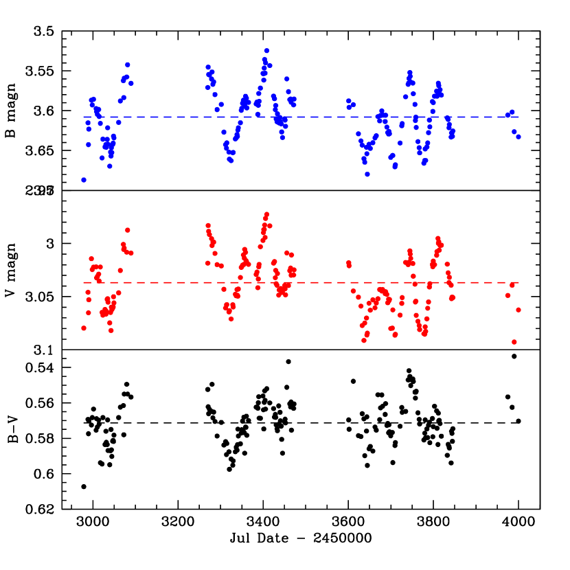
Figure 6: Model constraints for the primary of $\epsilon$ Aur involve both characteristics of the polarization variability as well as color variations. Shown here are $B$ and $V$ magnitudes at top and middle, with the $B-V$ color at bottom, used to characterize the color variations.

4.1 The Intrinsic Stellar Variability

The F star is a large and luminous star that is observed to vary outside of eclipse. As previously noted, it is a semi-regular variable with a characteristic period of about 100 days. In the V-band, the variations are of order a tenth of a magnitude relative to the mean. Those variations are accompanied by changes in $B-V$ color as well. Using data taken from the AAVSO, Figure 6 shows B and V band light curves, along with the variations in $B-V$, out of eclipse, and over about a 3-year span of time. The variations in $B-V$ have a standard deviation of $\sigma(B-V)=0.12$.

From Figure 1, the polarization out of eclipse is variable, with a time average of $\langle p\rangle=0.10\%$ over a span of about 4 years. During eclipse, the polarization is variable in a way that consists of the effect of the eclipse of the F star by the disk of the secondary along with the intrinsic variability of the F star. In addition, the $u$ light curve remains negative throughout the eclipse event, whereas the $q$ light curve tends to be positive, although it can change sign. In particular, the $q$ light curve is seen to become negative and remain negative during egress. The observed variations in $q$ and $u$ are reflected in the variation of the polarization position angle in the lowermost panel of Figure 1. There, $\psi_{P}$ is negative, hovering around $-50^{\circ}$, throughout the eclipse, and then becomes more randomized, with occasional rapid position angle changes, outside of eclipse.

The dispersion in the color of the F star, the average level of polarization outside of eclipse, and the distinctly different character of the variable polarization during eclipse as opposed to outside of eclipse are all features that we seek to reproduce with our model involving surface brightness variations. Note that our assumption is that neither the edge-on disk nor the secondary star contribute to the polarimetric variability. If either or both are sources of polarization, our modeling implicitly assumes those contributions are constant over the timespan of interest, and thus subsumed in the terms $\bar{q}$ and $\bar{u}$ as constant offsets for the variable component of the polarization.

4.2 Modeling Trends Outside of Eclipse

Recalling the illustrative examples, it is clear that a function $G$ involving only a single mode will not reproduce the observations for polarimetric variability outside of eclipse. A single mode yields a pattern that is too organized in a $q-u$ plot, whereas the observations lack such organization. The observations even lack a clear favored axis for the jumbled $q-u$ variations. As a result, we attempted to reproduce the observations using a combination of two modes. A good qualitative result was achieved with an equal combination of the (2,2) and (3,1) modes, with $G=0.5\,[G(2,2)+G(3,1)]$. This combination produces a pattern of $q-u$ variations that, although not a fit to the data, are similar in character.

Given those two modes, the next task was to simultaneously satisfy both the observed color variations and the observed average level of polarization. Figure 7 shows a grid of models use in determining the temperature parameters that satisfy the constraints. The figure is a plot of $T_{0}$ against $\Delta T^{4}/T_{0}^{4}$. The red contours are for $\sigma(B-V)$ with levels indicated next to each curve. The relevant contour for $\epsilon$ Aur is the one marked 0.012. The blue contours are for $\langle p\rangle$, again with levels indicated. The one relevant to $\epsilon$ Aur is 0.1%. The green circle indicates the intersection of the two relevant curves.

That solution has $\Delta T^{4}/T_{0}^{4}=0.33$ at $T_{0}\approx 7450$ K, the latter being close to the effective temperature of $7,395\pm 70$ K found by Strassmeier et al. (2014). Our result is specifically for a viewing inclination that is edge-on to the equator of the F star with $i=90^{\circ}$. The model adopts a limb polarization value of $p_{\cal L}=3\%$ at a temperature of 7400 K. A plot of the $q-u$ variations out of eclipse, that will be shown in conjunction with the variations during eclipse (see next section, and Fig. 8), were found to mimic the overall character of the observations.

For the variations in $B-V$, absolute magnitude $M_{B}$ and $M_{V}$ were used as functions of temperature from (Cox, 2000). A tabulation of $M_{V}$ and $B-V$ as functions of temperature for supergiant stars were used to construct intensities $I_{B}(T)$ and $I_{V}(T)$. At each time step in the model, the position-dependent intensities were integrated to form net fluxes $f_{B}(t)$ and $f_{V}(t)$, that were then combined to obtain colors $B-V$. Then $\sigma(B-V)$ was found from the simulated color curve. The set of contours shown in Figure 7 are for $\gamma_{0}=0.08$.

Note that the solution indicated in Figure 7 is not unique. For a given pattern function $G$, the contours for $\sigma(B-V)$ can be changed by altering the choice of $\gamma_{0}$. It is true that the effective temperature is constrained by observations at around 7,400 K; however, the dispersion in $B-V$ can be increased by increasing $\gamma_{0}$. Similarly, the contours for $\langle p\rangle$ can be shifted by altering the choice of $p_{\cal L}$. At a fixed value of $\Delta T^{4}/T_{0}^{4}$, the value of $\langle p\rangle$ will increase as $p_{\cal L}$ is increased. Naturally a unique solution is preferred. At this stage we may need to be satisfied with a plausible solution. That plausibility can be strengthened by considering whether the chosen parameters of the model can also explain the polarimetric behavior during the eclipse by the secondary’s disk, the topic of the next section.

4.3 Modeling The Eclipse Event

Kloppenborg et al. (2015) have conducted an extensive study of the occulting disk properties based on optical and infrared interferometric studies of $\epsilon$ Aur. Their disk model involves vertical and radial scale heights for the disk structure, along with opacities to compute absorbing optical depths as the eclipse evolves. Our study for the polarimetric variability during eclipse is less detailed and more proof-of-concept.

Table 1: Properties of $\epsilon$ Aur

Property	Value
Primarya	F0
Secondarya	BV(?)
$R_{1}/d^{a}$	$1.11\pm 0.05$ mas
$a/d^{a}$	$31.3\pm 3$ mas
$h_{D}/d^{a}$	$1.04\pm 0.14$ mas
$r_{D}/d^{a}$	$7.42\pm 0.28$ mas
$e^{b}$	$0.23\pm 0.01$
$P_{\rm orb}^{b}$	$9896\pm 1.6$ days
$i^{a}$	$89^{\circ}\pm 1^{\circ}$

^a from Kloppenborg et al. (2015)
^b from Stefanik et al. (2010)

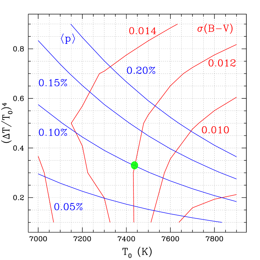
Figure 7: The model space of average temperature $T_{0}$ and amplitude for temperature perturbation $\Delta T$ with contours for the time variations in color $\sigma(B-V)$ (shown as red) and for the time-averaged polarization amplitude $\langle p\rangle$ (shown as blue). The green dot marks the location consistent with observations of $\epsilon$ Aur.

We adopt a simplified disk model for the eclipse consisting of a rectangular shape in projection. The disk has a long length in the orbital plane of $16R_{1}$, where $R_{1}$ is the radius of the F primary star. The full height of the rectangle can be treated as a free parameter of the model, but is reasonably constrained from the interferometric data during eclipse at about $1R_{1}$ (Kloppenborg et al., 2015). All rays that intercept the disk are taken to be completely occulted, so $\tau\rightarrow\infty$. The other free parameter for the eclipse event is the trajectory of the disk. The trajectory is actually comprised of two factors: (1) the impact parameter of the disk center relative to the star center in the plane of the sky, and (2) the orientation of the star’s spin axis relative to that trajectory. It is the latter that relates to the fact that the eclipse leads to a significant excursion of the polarization in the direction of negative Stokes-$u$.

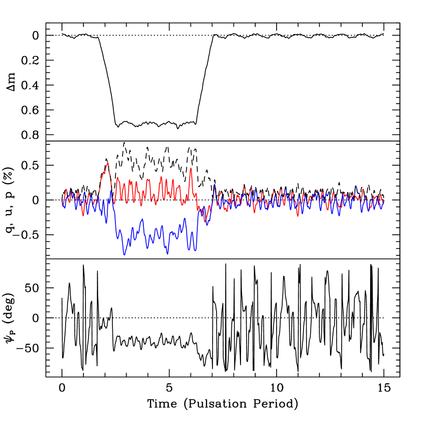
Figure 8: Model for the primary star and an eclipse by a disk about the secondary star using (2,2) and (3,1) modes of equal strength. Parameters for temperature and temperature variation are adopted from the solution (green dot) indicated in Fig. 7. The figure for the model replicates the style for the data displayed in Fig. 1.

Observations indicate that the disk runs across the lower half of the star during the eclipse event. This results in a drop of brightness of about 0.7 magnitudes in $V$. When running the disk parallel to the equator of the star, an excursion of the polarization, relative to outside of eclipse, does occur, but primarily in the direction of $q$. In order to obtain the observed excursion primarily in the direction of $u$, the star’s spin axis must be inclined significantly. While we take the F star as seen edge-on by observer, and we introduce an obliquity angle on the plane of the sky, $\psi_{\ast}$ between the spin axis and the normal to the disk. A value of $\psi_{\ast}=65^{\circ}$.

In the spirit of proof-of-concept, Figures 8 and 9 display model results that mimic the styles of Figures 1 and 2 for the observations reported by Henson (1989). The model results are for a disk that is $16R_{1}$ in diameter, with a height that is $0.75R_{1}$ as seen edge-on. The top of the disk, as projected against the F star, is $0.1R_{1}$ above the star center; the bottom of the disk stretches to $0.65R_{1}$ below star center. The periods involved are listed in Table 2. Mode switching (i.e., phase drift) occurs at the two relevant angular beat frequencies for $l=2$ and $l=3$, as previously discussed.

Table 2: Model Parameters for $\epsilon$ Aur

Property	Value
$T_{0}$	7,450 K
$\Delta T^{4}/T_{0}^{4}$	0.33
$\gamma_{0}$	0.08
$\psi_{\ast}$	$65^{\circ}$
$P_{\ast}$	1.0 years
$P_{0}$	0.30 years
$P_{2}$	0.17 years
$P_{3}$	0.094 years

Notable points for Figure 8 include the amount of eclipse in the light curve at approximate correct depth, along with variations in brightness at the level of a tenth of a magnitude (uppermost panel). From the middle panel, the $q$ and $u$ polarizations show complex behavior outside of eclipse. During eclipse, the $u$ polarization is notably shifted toward negative values. The $q$ polarization tends to be net positive, but can dip to small negative values as observed, and shows an excursion to the negative during egress. The polarization position angle (lowest panel) displays rapid position angle rotations outside eclipse, but hovers around $-50^{\circ}$ throughout the eclipse. These are all properties very like the observations.

Figure 9 shows the model results in a $q-u$ plot. The blue portion is for variations out of eclipse; the red is during the eclipse, with magenta corresponding to the ingress portion of the eclipse. The blue portion shows smoothly varying changes that are mostly randomly oriented. During eclipse, the polarization becomes larger, with a net excursion from the blue toward negative values of $u$. At the same time, there continue to be smoothly varying changes that are essentially centered on an offset position from the blue portion. This too is fairly similar to the observations. We note that the magenta portion is not represented in the data acquired by Henson (1989), as those observations began during the 1980’s eclipse, but after the ingress had passed. However, the observations obtained during the 2009-2011 eclipse by Henson et al. (2012) do indicate an excursion predominantly in $q$ during ingress. This gives additional support to the model reproducing the overall characteristics of the eclipse polarization.

One important note should be made about the modeling. The excursion to negative values of $u$ during eclipse requires that the spin axis of the star (from which the function $G$ for the temperature variations are defined) is inclined to the axis for the orbital plane of the binary. However, our modeling approach is meant to identify a size, amplitude, and pattern of brightness variations across the F star that can match the observed polarimetric data. The “spin axis” and mode switching serves merely to allow the brightness pattern to evolve. It is perhaps better to focus on the size scale of the surface variations and the timescale for how the pattern evolves. These are properties that could be tested against future interferometric observations.

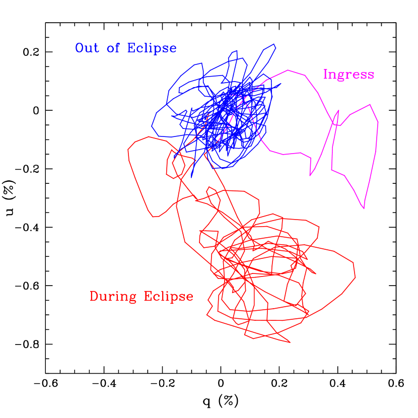
Figure 9: The is the $q-u$ plane for the model shown in Fig. 8. It uses the same style as for the data displayed in Fig. 2. The only difference is that $\bar{q}=\bar{u}=0$ for the model. The different colors are as labeled. Specifically, ingress is identified in magenta since that portion of the eclipse was part of the model but does not have a counterpart in the observational dataset obtained by Henson (1989), which began after ingress.

5 Summary

The match between the data and the model is by no means exact. It was not our intention to produce an actual fit to the data. What has been accomplished is that the characteristic observed variations (in shape and in amplitude) are broadly reproducible with our phenomenological model that is motivated by plausible expectations for the stellar atmosphere. Our model does have some degeneracies, such as the choice of limb polarization, and the amplitude for the time-dependence of the average surface temperature. More physically motivated, and therefore more numerically intensive, stellar atmosphere calculations are needed to obtain superior models in order to understand the variable nature of the F star. Those models will have consequences for better interpreting the eclipse event, with ramifications for understanding the disk and perhaps the history of this unusual system.

We point to one particular assumption that might be relaxed. Our model for brightness variations makes use of a temperature amplitude. The value needed to match the observations was $\Delta T^{4}/T_{0}^{4}=0.33$. At $T_{0}=7,450$ K, the implied range of temperatures across the star is rather large at 6,740–8,000 K. However, one assumption of the model is a fixed radius. Detailed atmosphere models reveal that late-type supergiants can deviate from spherical owing to convection. If such effects exist in the F star of $\epsilon$ Aur, then the distorted shape of the star alone would itself produce a net polarization. Combined with stellar rotation, the F star would display variable polarization even without temperature variations. Allowing for a variable shape of the star could reduce the amplitude of brightness variations (and in our model, temperature variations) across the atmosphere.

What does seem clear from our simplified approach is that (a) complex surface brightness variations are likely needed to explain the observed variable polarization data, (b) some modulation of the stellar temperature is likely needed to explain the observed color variations, and (c) and the distribution of brightness variations must evolve over time. These are features could be tested against new interferometric observations for better understanding the F star component of the $\epsilon$ Aurigae system.

References

- Al-Malki et al. (1999) Al-Malki, M. B., Simmons, J. F. L., Ignace, R., Brown, J. C., & Clarke, D. 1999, A&A, 347, 919
- Arellano Ferro (1985) Arellano Ferro, A. 1985, MNRAS, 216, 571
- Cassinelli & Hummer (1971) Cassinelli, J. P., & Hummer, D. G. 1971, MNRAS, 154, 9
- Clarke (2010) Clarke, D. 2010, Stellar Polarimetry
- Cole (2012) Cole, G. M. 2012, Journal of the American Association of Variable Star Observers (JAAVSO), 40, 787
- Cox (2000) Cox, A. N. 2000, Allen’s astrophysical quantities
- Doherty (1986) Doherty, L. R. 1986, ApJ, 307, 261
- Geise (2015) Geise, K. M. 2015, PhD thesis, University of Denver, Denver
- Gibson et al. (2018) Gibson, J. L., Stencel, R. E., Ketzeback, W., et al. 2018, MNRAS, 479, 2161
- Harrington (1970) Harrington, J. P. 1970, Ap&SS, 8, 227
- Henson (1989) Henson, G. D. 1989, PhD thesis, Oregon Univ., Eugene.
- Henson et al. (2012) Henson, G. D., Burdette, J., & Gray, S. 2012, in American Institute of Physics Conference Series, Vol. 1429, Stellar Polarimetry: from Birth to Death, ed. J. L. Hoffman, J. Bjorkman, & B. Whitney, 140–143
- Ignace et al. (2009) Ignace, R., Al-Malki, M. B., Simmons, J. F. L., et al. 2009, A&A, 496, 503
- Ikonnikova et al. (2018) Ikonnikova, N. P., Taranova, O. G., Arkhipova, V. P., et al. 2018, Astronomy Letters, 44, 457
- Karlsson (2012) Karlsson, T. 2012, Journal of the American Association of Variable Star Observers (JAAVSO), 40, 668
- Kemp & Barbour (1981) Kemp, J. C., & Barbour, M. S. 1981, PASP, 93, 521
- Kemp et al. (1986) Kemp, J. C., Henson, G. D., Kraus, D. J., et al. 1986, ApJ, 300, L11
- Kim (2008) Kim, H. 2008, Journal of Astronomy and Space Sciences, 25, 1
- Kloppenborg et al. (2015) Kloppenborg, B. K., Stencel, R. E., Monnier, J. D., et al. 2015, ApJS, 220, 14
- Kostogryz & Berdyugina (2015) Kostogryz, N. M., & Berdyugina, S. V. 2015, A&A, 575, A89
- Kostogryz et al. (2016) Kostogryz, N. M., Milic, I., Berdyugina, S. V., & Hauschildt, P. H. 2016, A&A, 586, A87
- Mourard et al. (2012) Mourard, D., Harmanec, P., Stencel, R., et al. 2012, A&A, 544, A91
- Neilson & Lester (2013a) Neilson, H. R., & Lester, J. B. 2013a, A&A, 554, A98
- Neilson & Lester (2013b) —. 2013b, A&A, 556, A86
- Osmer (1972) Osmer, P. S. 1972, ApJS, 24, 255
- Potravnov (2012) Potravnov, I. S. 2012, Astrophysics, 55, 528
- Stamford & Watson (1980) Stamford, P. A., & Watson, R. D. 1980, Acta Astron., 30, 193
- Stefanik et al. (2010) Stefanik, R. P., Torres, G., Lovegrove, J., et al. 2010, AJ, 139, 1254
- Stencel (2015) Stencel, R. E. 2015, ε Aurigae: A Two Century Long Dilemma Persists, ed. T. B. Ake & E. Griffin, Vol. 408, 107
- Strassmeier et al. (2014) Strassmeier, K. G., Weber, M., Granzer, T., et al. 2014, Astronomische Nachrichten, 335, 904