A Discrete-time Reputation-based Resilient Consensus Algorithm for Synchronous or Asynchronous Communications

Abstract

We tackle the problem of a set of agents achieving resilient consensus in the presence of attacked agents. We present a discrete-time reputation-based consensus algorithm for synchronous and asynchronous networks by developing a local strategy where, at each time, each agent assigns a reputation (between zero and one) to each neighbor. The reputation is then used to weigh the neighbors’ values in the update of its state. Under mild assumptions, we show that: (i) the proposed method converges exponentially to the consensus of the regular agents; (ii) if a regular agent identifies a neighbor as an attacked node, then it is indeed an attacked node; (iii) if the consensus value of the normal nodes differs from that of any of the attacked nodes’ values, then the reputation that a regular agent assigns to the attacked neighbors goes to zero. Further, we extend our method to achieve resilience in the scenarios where there are noisy nodes, dynamic networks and stochastic node selection. Finally, we illustrate our algorithm with several examples, and we delineate some attacking scenarios that can be dealt by the current proposal but not by the state-of-the-art approaches.

1 Introduction

In the last decades, much work has been devoted to networked control systems with a focus on cybersecurity aspects. Communications over shared mediums potentiates the exploitation of vulnerabilities that may result in consequences, sometimes, catastrophic.

A central problem in networked multi-agent systems is the so-called consensus problem, where a set of agents interacting locally through a communication network attempt to reach a common value. In other words, the final value is the outcome of running a distributed algorithm among nodes which can communicate according to the network topology. Therefore, the problem of consensus is the basilar stone of a multitude of applications, ranging areas such as: optimization [TBA86, JKJJ08]; motion coordination tasks – flocking and leader following [JLM03]; rendezvous problems [CMB06]; computer networks resource allocation [CLCD07]; and the computation of the relative importance of web pages, by PageRank like algorithm [SHS18a].

Notwithstanding, the consensus problem further appears as a critical subproblem of major applications. A distributed Kalman Filter based on two consensus systems was proposed in [OS07] to estimate the 2D motion of a target. The work was experimentally assessed in [AR07] to estimate the motion of a real robot. Due to the relevance of consensus methods and the cybersecurity aspects, a crucial property to ensure in any consensus algorithm is its ability to overcome abnormal situations, i.e., achieve resilient consensus.

Resilient consensus. Each agent in a network that works as expected must be able to filter erroneous information and be capable of reaching the consensus value that results from legit network information. A new fault-tolerant algorithm to accomplish approximate Byzantine consensus in asynchronous networks is introduced in [HA15a]. The method also applies to synchronous networks, to networks with communication paths with delay, and the authors extend the results to time-varying networks. Subsequently, authors performed the convergence rate analysis of the fault-tolerant consensus algorithm of [HA15a] in [HA15b].

The work in [SRC⁺13] introduced a system to tackle worst-case and stochastic faults in the particular scenario of gossip consensus. The developed method may be integrated into the consensus algorithm to achieve resilient consensus, making the nodes converge to a steady state belonging to the set resulting from the intersection of the estimates that each agent perceives for the remaining nodes [SRHS14]. The technique was extended to a wider family of gossip algorithms in [SRHS17]. These methods converge, and they offer a theoretical bound on the attacker signal, that can be computed a priori. However, their computational complexity for the worst-case undetectable attack makes the approach inviable. For detecting attacks, their computational complexity is, in general, worse than that of the new algorithm proposed in this work. For detecting attacks, their computational complexity is, in general, worse than that of the new algorithm proposed in this work. For attackers’ isolation, the computational complexity in [SRHS17, RSS20a, RSS20b] is exponential, contrasting with the proposed polynomial-time approach.

In [ÖA18], two fault-tolerant and parameter-independent consensus algorithms are introduced to deal with misbehaving agents. One of the approaches adaptively estimates, using a fault-detection scheme, how many faulty agents are in the network. Whenever there are $f$ faulty agents the authors’ method converges if the network of non-faulty nodes is $(f+1)$-robust. The other approach consists of a non-parametric Mean-Subsequence-Reduced algorithm, converging when both the network of non-faulty agents is $(f+1)$-robust and the non-faulty agents possess the same amount of in-neighbors.

In [SG18], the authors characterize the limitations on the performance of any distributed optimization algorithm in the presence of adversaries. Additionally, they investigated the vulnerabilities of consensus-based distributed optimization protocols to identify agents that are not following the consensus update rule. The authors suggest a resilient distributed optimization method, and they provide lower bounds on the distance-to-optimality of attainable solutions under any algorithm, resorting to the notion of maximal $f$-local sets of graphs for cases where each agent has at most $f$ adversaries neighbors.

In [DI15], the authors explore the scenario where each regular agent in a network refreshes its state based on local information, using a deliberated feedback law, and that malicious nodes update their state arbitrarily. The authors present an algorithm for the consensus of second-order sampled-data multi-agent systems. Assuming that the network has sufficient connectivity, the authors proposed a resilient consensus method, in which each node ignores the information of neighbors having large/small position values, considering that although the global topology of the network is unknown to regular agents, they know a priory the maximum number of malicious neighbor nodes. Next, using similar reasoning, the authors in [KDI18] extend the previous work, presenting a consensus algorithm for clock synchronization in wireless sensor networks.

Subsequently, in [Sun16], each agent may have a particular threshold for the number of extreme neighbors it ignores. Under such a setup, the author draws network conditions that ensure reaching a consensus. Further, the author presented conditions under which the consensus is asymptotically almost surely (with probability 1) achieved in random networks and with random node’s thresholds. In [UP18], it is proposed a resilient leader-follower consensus to arbitrary reference values, where each agent ignores a portion of extreme neighbors. This consensus method guarantees a steady state value lying in the convex hull of initial agent states. In a similar approach, the authors of [SPS⁺17] presented a resilient consensus algorithm for time-varying networks of dynamic agents. In [DIT17], the case of quantized transmissions, with communication delays and asynchronous update schemes is studied for update times selected in either a deterministic or random fashion.

In [CKM18], the authors present a consensus+innovations estimator. In the proposed method, each node in the network thresholds the gain to its innovations term. The authors ensure that if less than half of the agents’ sensors fall under attack, then all of the agents’ estimates converge with polynomial rate to the parameter of interest. In [DSI19], the authors present a resilient fully distributed averaging algorithm that uses a resilient retrieval procedure, where all non-Byzantine nodes send their initial values and retrieve those of other agents. The convergence is ensured under a more restrictive than the conventional node connectivities assumption.

Classes of consensus problems. We may classify the problems of consensus based on the domain of the time update as: discrete-time (discrete), as in [ZM10, CI12]; or as continuous-time (continuous), as in [RB05, CI12]. Also, it can be classified based on the network communication: synchronous, see for instance [ZM10]; or asynchronous, see for example [TBA86, HA15a, YAM⁺17]. Moreover, the communication between agents may be: deterministic, see [CI12] for example; or stochastic, as in [BGPS06, ASS11, SHS18b] for instance. Lastly, the agents’ network of communication can be categorized as: static, see [CI12, ÖA18, SHS18b]; or dynamic, changing in time, see in [OSM04, ZM10, SPS⁺17].

Here, we propose a resilient consensus algorithm that can be used for discrete-time, synchronous or asynchronous communication and static or dynamic network of communication. By synchronous we mean algorithms in which updates occur at the same time for all the nodes, whereas in an asynchronous setting, at each time, any non-empty subset of nodes may update their state.

Reputation systems. The concept of reputation of an entity is an opinion about that entity that usually results from an evaluation of the entity based on a set of criteria. Everyday, we implicitly assign a reputation to persons, companies, services, and many other entities. We do so by evaluating the entity behavior and comparing to what we would expect, and, further, by assessing other important (with large reputation) entities opinion. In fact, reputation is an ubiquitous, spontaneous and highly efficient utensil of social control in natural societies, emerging in business, education and online communities.

Hence, this ubiquitous concept has been ported to several important application with relative success, such as in ranking systems [LXYHC12, SRCK17b, SRCK17a, RB20], where reputation-based ranking systems are proposed and shown to cope better with attacks and to the effect of bribing. It is also an important measure to assess in the field of Social Networks as in [JIB07, ZNLY15]. In [PSD02], the authors propose a method to address the problem of calculating a degree of reputation for agents acting as assistants to the members of an electronic community.

For more related work on reputation systems, we refer the reader to the surveys in [JIB07, HBC15] and references therein.

Main contributions: (i) we propose a (fully distributed) discrete-time, reputation-based consensus algorithm resilient to attacks that works for both synchronous and asynchronous networks; with this algorithm, each agent only needs to have a low computational power to do calculations with the neighbors’ values; (ii) we show that the proposed algorithm converges with exponential rate; (iii) for attacks with some properties, we show, theoretically, that our method does not produce false positives and holds polynomial time complexity, although we observe the same behavior for other types of attacks.

1.1 Preliminaries and Terminology

First, we recall some concepts of graph theory, and we set the notation that we will adopt in this manuscript. A directed graph, or simply a digraph, is an ordered pair $\mathcal{G}=(\mathcal{V},\mathcal{E})$, where $\mathcal{V}$ is a set of $n>1$ nodes, and $\mathcal{E}\subseteq\mathcal{V}\times\mathcal{V}$ is a set of edges. Edges are ordered pairs which represent a relationship of accessibility between nodes. If $u,v\in\mathcal{V}$ and $(u,v)\in\mathcal{E}$ then the node $v$ directly accesses information of node $u$. In the scope of consensus algorithms, we also refer to a digraph as a network, and we further say that nodes are agents of the network. A complete digraph or complete network is a digraph such that all nodes can directly access information of every other node. Given an agent $v\in\mathcal{V}$, we denote the set of nodes that $v$ can directly access information in the network $\mathcal{G}=(\mathcal{V},\mathcal{E})$ by $\mathcal{N}_{v}=\{v\}\cup\{u\,:\,(u,v)\in\mathcal{E}\}$, and they are the neighbors of $v$. The proper neighbors of $v$ are $\bar{\mathcal{N}_{v}}=\mathcal{N}_{v}\setminus\{v\}$. The in-degree of a node $v\in\mathcal{V}$, denoted by $d_{v}$ is the number of neighbors of $v$, i.e., $d_{v}=|\mathcal{N}_{v}|$. Likewise, the out-degree of a node $v\in\mathcal{V}$, $o_{v}$, is the number of nodes that have $v$ has neighbor, i.e., $o_{v}=|\{u\,:\,v\in\mathcal{N}_{u}\}|$. A path in $\mathcal{G}=(\mathcal{V},\mathcal{E})$ is a sequence of nodes $(v_{1},v_{2},\ldots v_{k})$ such that $(v_{i},v_{i+1})\in\mathcal{E}$ for every $i=1,\ldots,k-1$. A convenient way of representing a digraph is by means of its adjacency matrix $A\in\mathbb{R}^{n\times n}$, where $A_{u,v}=1$ if $(u,v)\in\mathcal{E}$, and $A_{u,v}=0$, otherwise. A subgraph or a subnetwork $\mathcal{H}=(\mathcal{V}^{\prime},\mathcal{E}^{\prime})$ of a digraph $\mathcal{G}=(\mathcal{V},\mathcal{E})$ is a digraph such that $\mathcal{V}^{\prime}\subset\mathcal{V}$, $\mathcal{E}^{\prime}\subset\mathcal{E}$. If $\mathcal{A}$ denotes a set of nodes $\mathcal{A}\subset\mathcal{V}$, we denote by $\mathcal{G}\setminus\mathcal{A}$ the subgraph $\mathcal{H}$ of $\mathcal{G}$ that consists in $\mathcal{H}=(\mathcal{V}\setminus\mathcal{A},\mathcal{E}^{\prime})$, where $\mathcal{E}^{\prime}=\{e\in\mathcal{E}\,:\,e=(u,v)\text{ and }u,v\notin\mathcal{A}\}$.

Given a finite and non-empty array of possibly repeated elements sorted by increasing order $\mathcal{C}=\{x_{1},\ldots,x_{n}\}$, with $x_{i}\in\mathbb{R}$, with at least one $j\neq i$ and $x_{i}\neq x_{j}$, we define the following element: $\displaystyle\operatorname*{{min^{f}}}_{x\in\mathcal{C}}x=y_{f},$ where, inductively defined as

$$y_{f}={\small\begin{cases}x_{1},&\text{if }f=1\\[5.69046pt] \min\left\{x\in\mathcal{C}\,:\,y_{f-1}<x<x_{n}\right\},&\text{if }\displaystyle\mathop{\exists}_{x\in\mathcal{C}}y_{f-1}<x<x_{n}\\ y_{f-1},&\text{otherwise.}\end{cases}}$$

In other words, we are computing the $f$th smallest element of the set obtained from the array $\mathcal{C}$ by discarding repeated elements, but ensuring that it is not the maximum element. This definition will be very important to the reputation-based consensus method we propose, because we need to normalize a set of values, dividing them by the difference between the maximum and the $\operatorname*{{min^{f}}}$ element. For instance, consider the sets of sorted elements $\mathcal{C}=\{1,2,2,2,3\}$. If $f=1$ then $\displaystyle\operatorname*{{min^{f}}}_{x\in\mathcal{C}}x=1$, and if $f\geq 2$ then $\displaystyle\operatorname*{{min^{f}}}_{x\in\mathcal{C}}x=2$.

2 Reputation-Based Consensus

Consider a network of agents $\mathcal{G}=(\mathcal{V},\mathcal{E}^{(k)})$, with initial states $x_{v}^{(0)}\in\mathbb{R}$, for $v\in\mathcal{V}$. In the non-attacked scenario, agents can reach consensus through the use of a distributed linear iterative algorithm with dynamics given by:

$$x^{(k+1)}=W^{(k)}x^{(k)},$$ (1)

where $x^{(k)}$ is the vector collecting the $n$ agents states at time step $k>0$, and the matrix $W^{(k)}\in\mathbb{R}^{n\times n}$ is such that: (i) $W_{u,v}=0$ if the agents $u$ and $v$ do not communicate, and (ii) the agents converge to the same quantity, i.e., $\displaystyle\lim_{k\to\infty}x^{(k)}=x^{\infty}$.

Additionally, we consider a set of attacked agents $\mathcal{A}\subset\mathcal{V}$. If the agents $a\in\mathcal{A}$ do not follow the update rule of the consensus procedure, then each regular agent, $v\in\mathcal{V}\setminus\mathcal{A}$, should be able to identify and discard the attacked agents’ values in the computation of the consensus value. In order to solve the problem stated, we make the following assumption:

$\,\,\bullet\,\,$ For each regular agent, $v\in\mathcal{V}\setminus\mathcal{A}$, more than half of the neighbors are regular agents, i.e., $|\mathcal{N}_{v}\cap\mathcal{A}|<|\mathcal{N}_{v}|/2$ and the network of normal nodes is connected.

The assumption we made is a typical assumption in the state-of-the-art methods to achieve resilient consensus. We remark that the assumption we do make is equivalent to the $r$-robustness ($(r,1)$-robust) defined in [KDI18].

Further, observe that the previous assumption is reasonable, because each regular agent needs to be able to divide his neighbors into the set of normal nodes and the set of attacked ones, by comparing the information that it receives. Hence, if the majority of the information is not legitimate there is no redundancy to allow to identify the attacked neighbors.

2.1 Attacker model

In what follows, we consider an attacker that may corrupt the state of the nodes in the subset $\mathcal{A}$ by adding an unbounded signal. The attacked dynamics are a corrupted version of (1) as follows:

$$x^{(k+1)}=W^{(k)}x^{(k)}+\Delta^{(k)},$$ (2)

where $\Delta^{(k)}\in\mathbb{R}^{n}$, which entails the assumption that the attacker cannot corrupt the communication between nodes to send different messages to distinct neighbors. Observe that this assumption allows the attacker to change the state of a subset of agents to (possibly) different values. For example, in a network with 10 agents, an attacker may change the state of agents 3 and 5 using different values, but it cannot change the network communication scheme.

Furthermore, the attacker cannot create artificial nodes nor change the network topology, i.e., the structure of $W^{(k)}$ and the dimension $n$ are fixed in (2). Notice that if a malicious entity could create nodes in the network, it would be impossible to deter, as the attacked nodes would be the majority regardless of $n$.

Additionally, the attack cannot target the initial state, i.e., $\Delta^{(0)}=0$, since this scenario would be undetectable. The sequences of state values for the attacked version would be the same as a normal execution of the algorithm with the attack value as initial state.

2.2 Reputation-based consensus (RepC)

Next, we propose a reputation-based consensus algorithm (RepC). The idea behind the algorithm is that, each time an agent obtains information (states) from its neighbors, the agent measures how discrepant is, in average, the state from one neighbor regarding the states of the remaining ones and its own state. The RepC is composed by two phases: (i) identification of the attacked nodes; (ii) computation of the consensus.

Notice that the proposed algorithm is a fully distributed discrete-time consensus algorithm that works for both synchronous and asynchronous networks. Also, each agent only needs to have a low computational power to do calculations with the neighbors’ values.

2.2.1 Synchronous communication RepC

Given the maximum number of allowed attacked nodes $f$, the identification of the attacked nodes is performed by the following iterative scheme:

Reputation update:

$$\tilde{c}_{ij}^{(k+1)} =\begin{cases}1-\displaystyle\displaystyle\sum_{v\in\bar{\mathcal{N}_{i}}}\frac{|x_{j}^{(k)}-x_{v}^{(k)}|}{|\mathcal{N}_{i}|},&j\in\mathcal{N}_{i}\\ 0,&\text{otherwise}\end{cases}$$

Normalized Reputation update:

$$\tilde{\tilde{c}}_{ij}^{(k+1)} =\begin{cases}\displaystyle\frac{\tilde{c}_{ij}^{(k+1)}-\displaystyle\operatorname*{{min^{f}}}_{v\in\bar{\mathcal{N}_{i}}}\tilde{c}_{iv}^{(k+1)}}{\displaystyle\max_{v\in\bar{\mathcal{N}_{i}}}\tilde{c}_{iv}^{(k+1)}-\displaystyle\operatorname*{{min^{f}}}_{v\in\bar{\mathcal{N}_{i}}}\tilde{c}_{iv}^{(k+1)}},&i\neq j\\ 1,&\text{otherwise}\end{cases}$$

Normalized Reputation update with confidence $$\varepsilon$$:

$$c_{ij}^{(k+1)} =\begin{cases}\,\tilde{\tilde{c}}_{ij}^{(k+1)},&\text{if }\,\tilde{\tilde{c}}_{ij}^{(k+1)}>0,\\ \varepsilon^{k+1},&\text{otherwise}\\ \end{cases}$$

Consensus state update:

$$x_{i}^{(k+1)} =\displaystyle\sum_{j\in\bar{\mathcal{N}_{i}}}c_{ij}^{(k)}x_{j}^{(k)}\bigg{/}\displaystyle\sum_{j\in\bar{\mathcal{N}_{i}}}c_{ij}^{(k)},$$

$c_{ij}^{(k+1)}=0$ if $j\notin\mathcal{N}_{i}$, and $c_{ii}^{(k+1)}=1$, and where $c_{ij}^{(0)}=1$ for $j\in\bar{\mathcal{N}_{i}}$ and $c_{ij}^{(0)}=0$ otherwise, and $x_{i}^{(0)}$ is the initial value of each agent $i$. Further, $\varepsilon\in]0,1[$ is a confidence factor which guarantees that each agent does not discard immediately values that are discrepant from its neighbors’ average.

Notice that the selected value for $\varepsilon$ must be small to have a negligible impact on the agents’ consensus states. Also, a large $\varepsilon$ may cause an agent to do not detect an attacked neighbor. This, in turn, makes the asymptotic consensus to deviate from the consensus without attacked agents towards a combinations of the attacked agents asymptotic states. We illustrate this property in Section 3.

Further, notice that the proposed method computes a weighted average of the agents’ values. Therefore, we can ensure that the final consensus state is a convex combination of the agents’ initial states.

2.2.2 Asynchronous communication RepC

The asynchronous version of algorithm RepC consists of, at each instance of time, the agents that communicate, $\mathcal{A}^{\prime}\subset\mathcal{A}$, follow Equation (2.2.1), where $\bar{\mathcal{N}}_{i}$ is replaced by $\bar{\mathcal{N}}_{i}\cap\mathcal{A}^{\prime}$.

Another interesting fact is that the iterative scheme (2.2.1) may also be used in the scenario where the network of agents evolves with time. The results in Section 2.2 can be restated for this scenario by considering that the set of neighbors of a node is dynamic, and by verifying, at each time, that each agent has more than two neighbors and more than half of them are regular agents. In Section 3.4 and 3.5, we illustrate the dynamic network of agents and dynamic network with noisy agents scenarios.

The first important property to prove about RepC is that it converges. To simplify the proof, we assume that we are in the scenario of synchronous communication. The general proof follows the same steps, but it is more complex and it needs more complex notation to denote the set of neighbors with which a node communicates at each time. Additionally, we assume that $x_{i}^{(k)}\in[0,1]$. Notice that this corresponds to do a bijection of each $x_{i}^{(0)}$ as $\tilde{x}_{i}^{(0)}=(x_{i}^{(0)}-x_{\min}^{(0)})\big{/}(x_{\max}^{(0)}-x_{\min}^{(0)})$. Further, in the following proofs and for technical reasons, we assume that each attacked agent shares a state that is converging to some value. This simplification is needed in order to derive theoretical guarantees of the proposed method. Although, in practice, the algorithm is still effective under other circumstances, as we illustrate in Section 3.

Lemma 1.

If for any $i\in\mathcal{V}$ we have that $|\mathcal{N}_{i}|>2$, then each agent that follows the iterative scheme in (2.2.1) converges.

Proof.

$\left\|x^{(k+1)}-x^{(k)}\right\|_{\infty}=\displaystyle\max_{i}\left|x_{i}^{(k+1)}-x_{i}^{(k)}\right|$ and, hence, assuming without loss of generality that $\|c_{i}^{(k)}\|_{1}\leq\|c_{i}^{(k+1)}\|_{1}$

$$\left|x_{i}^{(k+1)}-x_{i}^{(k)}\right|=\left|\frac{c_{i}^{(k+1)}\cdot x^{(k)}}{\|c_{i}^{(k+1)}\|_{1}}-\frac{c_{i}^{(k)}\cdot x^{(k-1)}}{\|c_{i}^{(k)}\|_{1}}\right|$$

$$=\left|\frac{c_{i}^{(k+1)}\cdot x^{(k)}}{\|c_{i}^{(k+1)}\|_{1}}-\frac{c_{i}^{(k)}\cdot x^{(k)}}{\|c_{i}^{(k+1)}\|_{1}}+\frac{c_{i}^{(k)}\cdot x^{(k)}}{\|c_{i}^{(k+1)}\|_{1}}-\frac{c_{i}^{(k)}\cdot x^{(k-1)}}{\|c_{i}^{(k)}\|_{1}}\right|$$

$$\leq\left|\frac{c_{i}^{(k+1)}\cdot x^{(k)}}{\|c_{i}^{(k+1)}\|_{1}}-\frac{c_{i}^{(k)}\cdot x^{(k)}}{\|c_{i}^{(k+1)}\|_{1}}+\frac{c_{i}^{(k)}\cdot x^{(k)}}{\|c_{i}^{(k)}\|_{1}}-\frac{c_{i}^{(k)}\cdot x^{(k-1)}}{\|c_{i}^{(k)}\|_{1}}\right|$$

$$=\left|\frac{c_{i}^{(k+1)}-c_{i}^{(k)}}{\|c_{i}^{(k+1)}\|_{1}}\cdot x^{(k)}+c_{i}^{(k)}\cdot\frac{x^{(k)}-x^{(k-1)}}{\|c_{i}^{(k)}\|_{1}}\right|$$

$$\leq\frac{\max_{j\in\mathcal{N}_{i}}|c_{ij}^{(k+1)}-c_{ij}^{(k)}|}{\|c_{i}^{(k+1)}\|_{1}}+\frac{\max_{j\in\mathcal{N}_{i}}|x_{j}^{(k)}-x_{j}^{(k-1)}|}{\|c_{i}^{(k)}\|_{1}}$$

$$\leq\frac{\max_{j\in\mathcal{N}_{i}}|c_{ij}^{(k+1)}-c_{ij}^{(k)}|}{\|c_{i}^{(k)}\|_{1}}+\frac{\max_{j\in\mathcal{N}_{i}}|x_{j}^{(k)}-x_{j}^{(k-1)}|}{\|c_{i}^{(k)}\|_{1}},$$

because we are assuming that $x_{v}^{(m)},c_{ij}^{(m)}\in]0,1[$. Now we need to compute $\max_{j\in\mathcal{N}_{i}}|c_{ij}^{(k+1)}-c_{ij}^{(k)}|$. First, we notice that we cannot have that $\max_{j\in\mathcal{N}_{i}}|c_{ij}^{(k+1)}-c_{ij}^{(k)}|=|\varepsilon^{k+1}-\varepsilon^{k}|$, because there is always a $j\in\mathcal{N}_{i}$ such that $c_{ij}^{(k+1)}>\varepsilon^{k+1}$ and all the other $k\neq j\in\mathcal{N}_{i}$ are such that $c_{ij}^{(k+1)}\geq\varepsilon^{k+1}$. Therefore, we need to consider only three cases:

1. $c_{ij}^{(k+1)}=\varepsilon^{k+1}$ and $c_{ij}^{(k)}=\tilde{\tilde{c}}_{ij}^{(k)}$;

2. $c_{ij}^{(k+1)}=\tilde{\tilde{c}}_{ij}^{(k+1)}$ and $c_{ij}^{(k)}=\varepsilon^{k}$;

3. $c_{ij}^{(k+1)}=\tilde{\tilde{c}}_{ij}^{(k+1)}$ and $c_{ij}^{(k)}=\tilde{\tilde{c}}_{ij}^{(k)}$.

For case $1)$ we have that $\left|c_{ij}^{(k+1)}-c_{ij}^{(k)}\right|=\left|\varepsilon^{k+1}-\tilde{\tilde{c}}_{ij}^{(k)}\right|<\left|\,\tilde{\tilde{c}}_{ij}^{(k+1)}-\tilde{\tilde{c}}_{ij}^{(k)}\right|,$ since $c_{ij}^{(k+1)}=\varepsilon^{k+1}$ implies that $\tilde{\tilde{c}}_{ij}^{(k+1)}\leq 0$. Using the same reasoning, for case $2)$, we have that $\left|c_{ij}^{(k+1)}-c_{ij}^{(k)}\right|=\left|\,\tilde{\tilde{c}}_{ij}^{(k+1)}-\varepsilon^{k}\right|<\left|\,\tilde{\tilde{c}}_{ij}^{(k+1)}-\tilde{\tilde{c}}_{ij}^{(k)}\right|.$ We only need to compute $3)$

$$\begin{split}\left|\,\tilde{\tilde{c}}_{ij}^{(k+1)}-\tilde{\tilde{c}}_{ij}^{(k)}\right|=\frac{\left|\tilde{c}_{ij}^{(k+1)}-\tilde{c}_{ij}^{(k)}\right|}{\max_{v\in\bar{\mathcal{N}_{i}}}\tilde{c}_{iv}^{(k+1)}-\operatorname*{{min^{f}}}_{v\in\bar{\mathcal{N}_{i}}}\tilde{c}_{iv}^{(k+1)}}\\ \leq|\tilde{c}_{ij}^{(k+1)}-\tilde{c}_{ij}^{(k)}|\\ =\frac{1}{|\bar{\mathcal{N}_{i}}|}\sum_{v\in\bar{\mathcal{N}_{i}}}\left(|x_{j}^{(k)}-x_{v}^{(k)}|-|x_{j}^{(k-1)}-x_{v}^{(k-1)}|\right)\\ \leq\frac{1}{|\mathcal{N}_{i}|}|\mathcal{N}_{i}|\left(|x_{j}^{(k)}-x_{\alpha}^{(k)}|-|x_{j}^{(k-1)}-x_{\alpha}^{(k-1)}|\right)\\ =\left(|x_{j}^{(k)}-x_{\alpha}^{(k)}|-|x_{\alpha}^{(k-1)}-x_{j}^{(k-1)}|\right.\\ +\left.|x_{\alpha}^{(k-1)}-x_{j}^{(k-1)}|-|x_{j}^{(k-1)}-x_{\alpha}^{(k-1)}|\right)\\ \leq\left(|x_{j}^{(k)}-x_{j}^{(k-1)}|+|x_{\alpha}^{(k)}-x_{\alpha}^{(k-1)}|\right)\leq 2\displaystyle\max_{j\in\bar{\mathcal{N}_{i}}}|x_{j}^{(k)}-x_{j}^{(k-1)}|,\end{split}$$ (3)

where $\alpha=\displaystyle\underset{v\in\bar{\mathcal{N}_{i}}}{\arg\max}\left(|x_{j}^{(k)}-x_{v}^{(k)}|-|x_{j}^{(k-1)}-x_{v}^{(k-1)}|\right)$. Now, plugging (3) in (2.2.2), we have that

$${\small\begin{split}\|x^{(k+1)}-x^{(k)}\|_{\infty}\leq\frac{3}{\|c_{i}^{(k))}\|_{1}}\max_{j\in\bar{\mathcal{N}_{i}}}|x_{j}^{(k)}-x_{j}^{(k-1)}|\\ \leq\frac{3}{\|c_{i}^{(k)}\|_{1}}\|x^{(k)}-x^{(k-1)}\|_{\infty}\leq\frac{3}{|\bar{\mathcal{N}_{i}}|}\|x^{(k)}-x^{(k-1)}\|_{\infty}\end{split}}$$

Therefore, the iterative scheme converges whenever $\frac{3}{|\mathcal{N}_{i}|+1}<1$, which is equivalent to $|\mathcal{N}_{i}|>2$. ∎

In fact, the requirement about the number of neighbors, i.e., each agent having more than 2 neighbors, agrees with the intuition. A regular agent should assess to, at least, 3 states to distinguish whether nodes are following the consensus update rule or not. Otherwise, if there are only 2 neighbors then their reputation can be, for instance, alternating between iterations.

The previous result states that RepC converges (i.e. each agent converges to a state) but it is still missing to show that each regular agent converges to the same value, i.e., all regular agents agree. The next lemma assesses that: (i) either an agent $v$ converges to a unique value; (ii) or for any other agent, the reputation of agent $v$ is zero, i.e. $c_{uv}^{\infty}=0$.

Lemma 2.

Consider the iterative scheme 2.2.1. For any agent $j\in\mathcal{V}$ one of the following holds:

1. $\displaystyle\lim_{k\to\infty}x_{j}^{(k)}=x^{\infty}$;

2. $\displaystyle\forall_{i\in\mathcal{N}_{j}}\lim_{k\to\infty}c_{ij}^{(k)}=0$ (neighbors of $j$ assign it reputation zero).

Proof.

By Lemma 1, we have that (2.2.1) converges for each agent $i\in\mathcal{V}\setminus\mathcal{A}$. We just need to show that for a given node $u\in\mathcal{V}\setminus\mathcal{A}$ and for each of its neighbors $v\in\mathcal{N}_{u}$ either $(i)$ or $(ii)$ happens. Let $u\in\mathcal{V}\setminus\mathcal{A}$ and $v\in\mathcal{N}_{u}$, we show by induction on the number of neighbors of $u$, $|\mathcal{N}_{u}|$, that for each neighbor either its reputation is zero or it converges to the same value as $u$. The basis is when $|\mathcal{N}_{u}|=1$, and we have that $x^{\infty}_{u}=\frac{x^{\infty}_{u}+c^{\infty}_{uv}x_{v}^{\infty}}{1+c^{\infty}_{uv}}$. Thus, either $c^{\infty}_{uv}=0$, or $c^{\infty}_{uv}>0$ and $x_{v}^{\infty}=x_{u}^{\infty}$. When $|\mathcal{N}_{u}|=N+1$, we have that $x^{\infty}_{u}=\sum_{j\in\bar{\mathcal{N}}_{u}}c_{uj}^{\infty}x_{j}^{\infty}\bigg{/}\sum_{j\in\bar{\mathcal{N}}_{u}}c_{uj}^{\infty}.$ Since the reputation that $u$ assigns to itselft is $c^{\infty}_{uu}=1$, we can rewrite the previous expression as

$$x^{\infty}_{u}=\frac{x_{u}^{\infty}+\sum_{j\in\mathcal{N}_{u}\setminus\{v\}}c_{uj}^{\infty}x_{j}^{\infty}+c_{uv}^{\infty}x_{v}^{\infty}}{1+\sum_{j\in\mathcal{N}_{u}\setminus\{v\}}c_{uj}^{\infty}+c_{uv}^{\infty}}$$ (4)

Further, using the induction hypothesis, either $(i)$ or $(ii)$ is true for any set of $N$ neighbors of $u$. Hence, for $j\in\mathcal{N}_{u}\setminus\{v\}$ either $x_{j}^{\infty}=x^{\infty}$ or $c_{uj}^{\infty}=0$. In any of the cases, we have that

$$x_{u}^{\infty}+\sum_{j\in\mathcal{N}_{u}\setminus\{v\}}c_{uj}^{\infty}x_{j}^{\infty}=x^{\infty}\left(1+\sum_{j\in\mathcal{N}_{u}\setminus\{v\}}c_{uj}^{\infty}\right)$$ (5)

By replacing (5) in (4), it follows that

$${\small\begin{split}x^{\infty}_{u}=x^{\infty}&=\frac{x^{\infty}\left(1+\sum_{j\in\mathcal{N}_{u}\setminus\{v\}}c_{uj}^{\infty}\right)+c_{uv}^{\infty}x_{v}^{\infty}}{\left(1+\sum_{j\in\mathcal{N}_{u}\setminus\{v\}}c_{uj}^{\infty}\right)+c_{uv}^{\infty}},\\ \end{split}}$$

implying that either $c_{uv}^{\infty}=0$ or $c_{uv}^{\infty}>0$ and $x_{v}^{\infty}=x_{u}^{\infty}=x^{\infty}$. By transitivity, we can apply the same to each neighbor of all neighbors of $u$, and so forth. Thus, the result yields for all $i\in\mathcal{V}\setminus\mathcal{A}$. ∎

As a corollary, we have that if a regular agent using RepC detects a neighbor as a faulty node, then it is a faulty node. In other words, there are no false positives.

Corollary 1.

Let $v\in\mathcal{V}\setminus\mathcal{A}$ and $u\in\mathcal{V}$. By using the iterative scheme (2.2.1), if $c_{uv}^{\infty}=0$ then $u\in\mathcal{A}$.

The proof of Lemma 1 also hints that half of each agent’s neighbors should not be under attack, so that each normal node identifies the attacked agents correctly. This is expressed in the following.

Lemma 3.

Suppose that the iterative scheme (2.2.1) converges to a value different from that broadcasted by the attacked agents. If for each agent $i\in\mathcal{V}\setminus\mathcal{A}$, less than half of its neighbors are not attacked agents, i.e. $|\bar{\mathcal{N}_{i}}\cap\mathcal{A}|<|\bar{\mathcal{N}_{i}}\setminus\mathcal{A}|$, then $\displaystyle\lim_{k\to\infty}c_{ia}^{(k)}=0$, for $a\in\mathcal{A}$ and $\displaystyle\lim_{k\to\infty}c_{iv}^{(k)}=1$ for $v\in\bar{\mathcal{N}_{i}}\setminus\mathcal{A}$.

Proof.

By Lemma 1, we have that the each regular agent using the iterative scheme in (2.2.1) converges to $x^{\infty}$. Let $y$ denote the value that all the attacked agents in $\mathcal{A}$ share with the neighbors. Thus, for a regular agent $i\notin\mathcal{A}$, an attacked agent’s reputation, $a\in\mathcal{A}$, satisfies

$${\small\begin{split}\tilde{c}_{ia}^{\infty}=&\lim_{k\to\infty}\tilde{c}_{ia}^{(k)}=1-\frac{1}{|\mathcal{N}_{i}|}\sum_{v\in\mathcal{N}_{i}}\left|y-\lim_{k\to\infty}x_{v}^{(k)}\right|\\ =&1-\frac{|\mathcal{N}_{i}\setminus\mathcal{A}|}{|\mathcal{N}_{i}|}\left|y-x^{\infty}\right|,\end{split}}$$

and the limit of the reputation of a regular user, $j\notin\mathcal{A}$, is given as

$$\tilde{c}_{ij}^{\infty}=\lim_{k\to\infty}\tilde{c}_{ij}^{(k)}=1-\frac{|\mathcal{N}_{i}\cap\mathcal{A}|}{|\mathcal{N}_{i}|}\left|x^{\infty}-y\right|.$$

Since $|\mathcal{N}_{i}\cap\mathcal{A}|<|\mathcal{N}_{i}\setminus\mathcal{A}|$ and $y\neq x^{\infty}$, then $\tilde{c}_{ij}^{\infty}>\tilde{c}_{ia}^{\infty}$, and because reputations values are normalized to be between $0$ and $1$, we have that, for all $i$, $1=c_{ij}^{\infty}>c_{ia}^{\infty}=0$. ∎

Now, we need to show that a regular agent using RepC identifies the neighbors which are attacked nodes, and to study the convergence rate of method.

Lemma 4.

Let $v\in\mathcal{V}\setminus\mathcal{A}$ and $u\in\mathcal{V}$. By using the iterative scheme (2.2.1), if $u\in\mathcal{A}$ and $|\mathcal{A}|\leq f$ then $c_{uv}^{\infty}=0$.

Proof.

Let $a\in\mathcal{A}$ be an attacked node. We want to show that for a regular agent, $v\in\mathcal{V}\setminus\mathcal{A}$, the reputation of agent $a$ strictly decreases with time. Let $v\in\mathcal{V}\setminus\mathcal{A}$, we have that $|x_{a}-x_{v}^{(k+1)}|-|x_{a}-x_{v}^{(k)}|\leq|x_{v}^{(k+1)}-x_{v}^{(k)}|.$ ∎

Proposition 1.

Consider the iterative scheme in (2.2.1) and let $N=\displaystyle\min_{i\in\mathcal{V}}|\mathcal{N}_{i}|$ and $\lambda=\frac{3}{N+1}$. If $N>3$, then (2.2.1) converges with exponential rate and we have that $\|x^{(k+1)}-x^{(k)}\|_{\infty}\leq\lambda^{k}$. Further, to achieve an error of at most $\delta>0$ between the last two iterations, we need to run the iterative scheme at most $k=\lceil\log_{\lambda}(\delta)\rceil$ times.

Proof.

Let $N=\displaystyle\min_{i\in\mathcal{V}}|\mathcal{N}_{i}|$ and $\lambda=\frac{3}{N+1}$. Using the proof of Lemma 1, we have that $\|x^{(k+1)}-x^{(k)}\|_{\infty}\leq\frac{3}{|\bar{\mathcal{N}_{i}}|}\|x^{(k)}-x^{(k-1)}\|_{\infty}\leq\lambda^{k}\|x^{(1)}-x^{(0)}\|_{\infty}\leq\lambda^{k}.$ Hence, the iterative scheme converges with exponential rate of $\lambda^{k}$. To achieve an error between iterations of at most $\varepsilon$, we need to have that $\lambda^{k}\leq\delta,$ which is equivalent to have that $k\leq\log_{\lambda}(\delta)\leq\lceil\log_{\lambda}(\delta)\rceil.$ Therefore, if we run the iterative scheme at most $\lceil\log_{\lambda}(\delta)\rceil$ times, we obtain an error between the last two iterations of at most $\varepsilon$. ∎

2.3 Complexity Analysis

Next, we investigate the complexity analysis of the proposed algorithm RepC, when the network communication is synchronous.

Proposition 2.

Let $\mathcal{G}=(\mathcal{V},\mathcal{E})$ be a network of agents, $l=\displaystyle\max_{v\in\mathcal{V}}|\mathcal{N}_{v}|$, then, for $i$ iterations and for each agent, the iterative scheme (2.2.1) has time complexity of $\mathcal{O}(l^{2}i)$.

Proof.

Given a network of agents $\mathcal{G}=(\mathcal{V},\mathcal{E})$, for time step $k$ and for an agent $v$, the time complexity of (2.2.1) is the sum of the time complexities of computing $\tilde{c}_{vu}^{(k)}$, $\tilde{\tilde{c}}_{vu}^{(k)}$, $c_{vu}^{(k)}$, for each $u\in\mathcal{N}_{i}$, and $x_{v}^{(k)}$. Computing $\tilde{c}_{vu}^{(k)}$ has computation complexity of $\mathcal{O}(|\mathcal{N}_{v}|^{2})$, because there are $\mathcal{O}(|\mathcal{N}_{v}|^{2})$ pairs of neighbors values to compute the absolute difference. Each of the remaining steps has time complexity of $\mathcal{O}(|\mathcal{N}_{v}|)$. Hence, the sum of each step time complexity is $O(|\mathcal{N}_{v}|^{2})+4\times\mathcal{O}(|\mathcal{N}_{v}|)=O(|\mathcal{N}_{v}|^{2})$. Thus, if $l=\displaystyle\max_{v\in\mathcal{V}}|\mathcal{N}_{v}|$, then $\mathcal{O}(l^{2})$ is a bound for the time complexity that each incurs. Therefore, for $i$ iterations of the iterative scheme (2.2.1), each agent incurs in $\mathcal{O}(l^{2}i)$ time complexity. ∎

3 Illustrative Examples

Subsequently, we illustrate the use of RepC for different kinds of attacks. Further, in the examples, we use $\varepsilon=0.1$.

3.1 Same value for attacked nodes

In the following examples, we consider the network of agents depicted in Fig. 1 (a).

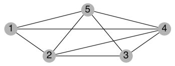
(a) Network of agents $\mathcal{G}_{A}$.

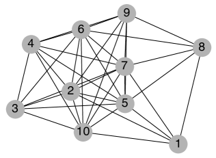
(b) Network of agents $\mathcal{G}_{B}$.

Figure 1:

First, we illustrate algorithm RepC in the scenario of a network of agents without attacked nodes. The set of agents is $\mathcal{V}_{1}=\{1,\ldots,5\}$ and, thus, the set of attacked agents is $\mathcal{A}=\emptyset$. We set the parameter $f=1$. Figure 2 depicts the state evolution of each agent.

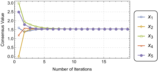
Figure 2: Consensus of network $\mathcal{G}_{A}$ with agents $\mathcal{V}_{1}$ and set of attacked agents $\emptyset$.

Here, we explore the scenario where an attacker targets one agent to share a value close to the consensus of the network of regular agents, depicted in Fig. 1.

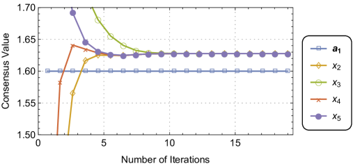
Figure 3: Consensus of network $\mathcal{G}_{A}$ with agents $\mathcal{V}_{1}$ and set of attacked agents $\mathcal{A}_{1}$ (zoomed around the attacker’s value.)

The set of agents is $\mathcal{V}=\{1,\ldots,5\}$ and the set of attacked agents is $\mathcal{A}=\{1\}$. Figure 3 depicts each agent consensus value. We can see that although the attacker value is very close to the consensus value, the neighbors of the attacked node assign zero to its reputation, by using (2.2.1). Hence the value that the attacked node shares is discarded.

Next, in Figure 4 – Fig. 5, we depict the evolution of the reputations that agents $2$ and $3$ assign to their neighbors.

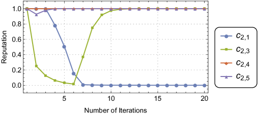
Figure 4: Evolution of the reputations that agent $2$ assigns to each of its neighbors.

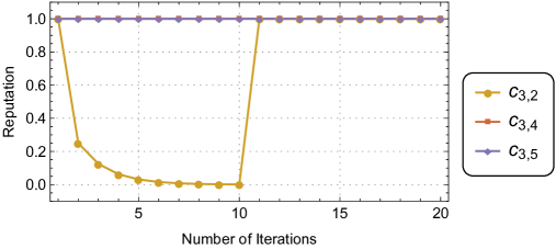
Figure 5: Evolution of the reputations that agent $3$ assigns to each of its neighbors.

3.2 Different values for attacked nodes

Next, we illustrate the scenario where attacked nodes share different values. For that end, we consider the set of agents $\mathcal{V}=\{1,\ldots,10\}$, with $\mathcal{A}=\{1,8\}$, and the network of agents depicted in Fig. 1 (b). We explore two scenarios with two attacked agents: (i) both attacked nodes share values (distinct) smaller than the consensus, see Fig. 6; (ii) one attacked node shares a value larger than the consensus while the other uses a smaller value than the consensus, see Fig. 7.

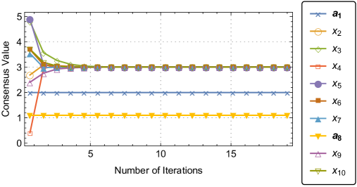
Figure 6: Consensus of network $\mathcal{G}_{B}$ with agents $\mathcal{V}_{3}$ and set of attacked agents $\mathcal{A}_{3}$

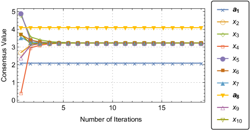
Figure 7: Consensus of network $\mathcal{G}_{B}$ with agents $\mathcal{V}_{2}$ and set of attacked agents $\mathcal{A}_{2}$

3.3 Asynchronous Communication

We, now, illustrate the use of algorithm RepC in the case where the communication between nodes occur asynchronously. To simulate this scenario, at each time instance, a random subset of agents communicates. The set of agents is $\mathcal{V}=\{1,\ldots,5\}$, the network of agents is $\mathcal{G}_{A}$, and the set of attacked agents is $\mathcal{A}=\{1\}$. Figure 8 depicts the state evolution of each agent when using the asynchronous version of algorithm RepC. Each normal node identifies and discards the information of the attacked agent.

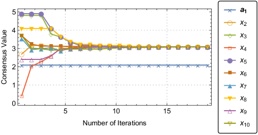
Figure 8: Consensus of network $\mathcal{G}_{A}$ with agents $\mathcal{V}_{1}$, asynchronous communication, and set of attacked agents $\mathcal{A}=\{1\}$.

3.4 Dynamic network

Next, we test the scenario where the network of agents evolves with time and the attacked agents share the same value. We consider two networks composed by 10 agents, as depicted in Fig. 9, with set of agents $\mathcal{V}=\{1,\ldots,10\}$ and set of attacked agents $\mathcal{A}=\{1\}$.

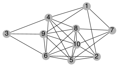
(a) Network of agents $\mathcal{G}_{D}$.

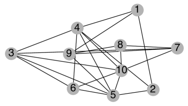
(b) Network of agents $\mathcal{G}_{C}$.

Figure 9:

In the example, we consider that the dynamic network of agents for time instance $k>0$ is given by $\mathcal{G}_{1}^{(k)}=\begin{cases}\mathcal{G}_{C}&\text{if }k\leq 10\\ \mathcal{G}_{D}&\text{otherwise}\end{cases}.$ The consensus value of each agent, utilizing the iterative scheme (2.2.1), is depicted in Fig. 10.

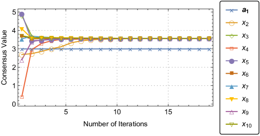
Figure 10: Consensus of dynamic network $\mathcal{G}_{1}^{(k)}$ with agents $\mathcal{V}_{1}$, and set of attacked agents $\mathcal{A}=\{1\}$.

3.5 Dynamic network with noisy agents

Finally, we illustrate the scenario where not only the network of agents evolves with time, but also the attacked agents share different values, which are uniform random variables with a fixed mean value. These is captured in the example depicted in Fig. 11.

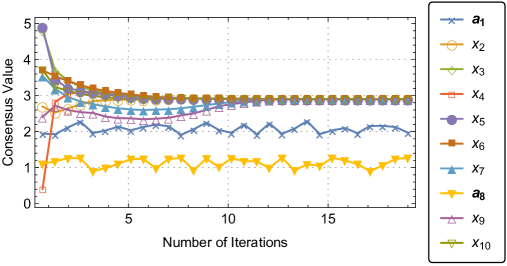
Figure 11: Consensus of dynamic network $\mathcal{G}_{1}^{(k)}$ with agents $\mathcal{V}_{1}$, and set of attacked (noisy) agents $\mathcal{A}=\{1,8\}$.

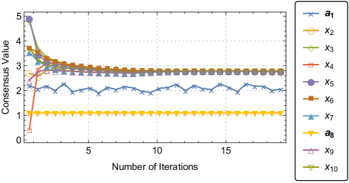
Figure 12: Consensus of dynamic network $\mathcal{G}_{1}^{(k)}$ with agents $\mathcal{V}_{1}$, and set of attacked agents $\mathcal{A}=\{1,8\}$, where agent $1$ behaves as a noisy node and agent $8$ as an attacked node.

3.6 Stochastic communication

When the communication between agents has a stochastic nature, we may still successfully apply RepC. This is illustrated in the next example. We consider the network $\mathcal{G}_{E}$ in Fig. 13, with $\mathcal{V}_{1}$, and the set of attacked agents $\mathcal{A}=\{1\}$. Further, at each time step, only a random subset of agents communicate between them. The described situation is depicted in Fig. 14, where the regular agents could effectively detect the attacked node and achieve the true consensus of the network.

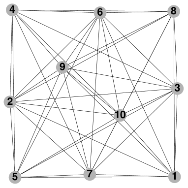
Figure 13: Network of agents $\mathcal{G}_{E}$.

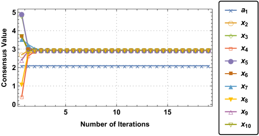
Figure 14: Consensus using a RepC method, with network $\mathcal{G}_{E}$, set of agents $\mathcal{V}_{1}$, set of attacked agents $\mathcal{A}=\{1\}$ and stochastic communication.

3.7 RepC vs. state-of-the-art

Here, we illustrate how the proposed algorithm competes with the state-of-the-art approaches, based on the idea that each agent discards a set of maximum and minimum neighbor values.

In the next examples, we use the two networks depicted in Fig. 15.

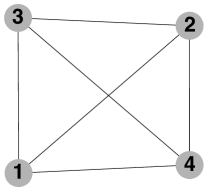
(a) Network of agents $\mathcal{G}_{F}$.

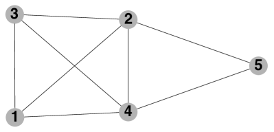
(b) Network of agents $\mathcal{G}_{G}$.

Figure 15:

In the first example, consider the set of agents $\mathcal{V}_{2}=\{1,2,3,4\}$, with the complete network (Fig. 15 (a)) and attacked agents $\mathcal{A}=\{1\}$.

Using the state-of-the-art, i.e., when each agent discards the maximum and minimum neighbors’ values, we obtain the result depicted in Fig. 16. The method is not able to deter the attack and the regular agents converge to the attacker value.

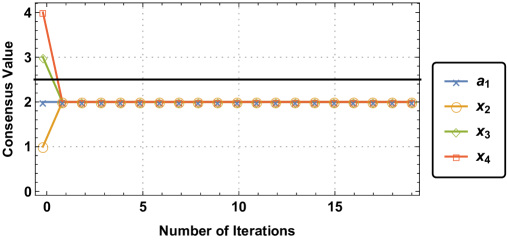
Figure 16: Consensus using a state-of-the-art method, with network $\mathcal{G}_{F}$, set of agents $\mathcal{V}_{2}$, and set of attacked agents $\mathcal{A}=\{1\}$. The black line is the true consensus value.

Using RepC, as illustrated in Fig. 17, the regular agents converge to a value close to the true value, with a small deviation caused by the influence of the $\varepsilon$ parameter.

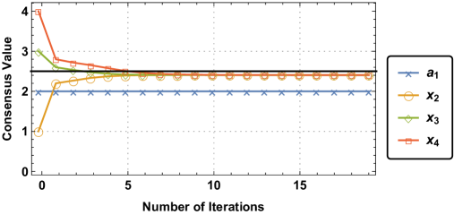
Figure 17: Consensus using RepC, with network $\mathcal{G}_{F}$, set of agents $\mathcal{V}_{2}$, and set of attacked agents $\mathcal{A}=\{1\}$. The black line is the true consensus.

In the second example, we consider the network of agents depicted in Fig. 15 (b), the set of agents $\mathcal{V}_{3}=\{1,2,3,4,5\}$ and attacked agents set $\mathcal{A}=\{1\}$. The example portraits the scenario where an attacker stubbornly sends to the neighbors the true consensus value.

In Fig. 18, we present the consensus states of the agents when using the state-of-the-art approach. We can see that the agents are not able to converge to the true consensus value.

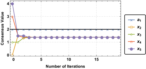
Figure 18: Consensus using a state-of-the-art method, with network $\mathcal{G}_{G}$, set of agents $\mathcal{V}_{3}$, and set of attacked agents $\mathcal{A}=\{1\}$. The black line is the true consensus value.

Subsequently, we present the consensus state of the agents when using RepC. In this case, the agents are able to converge to the true consensus of the network.

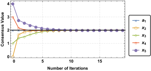
Figure 19: Consensus using RepC, with network $\mathcal{G}_{F}$, set of agents $\mathcal{V}_{3}$, and set of attacked agents $\mathcal{A}=\{1\}$. The black line is the true consensus.

3.8 Consensus final error

To explore how different is the final consensus value produced by RepC and the consensus value without attacked nodes, we use the complete network of $5$ agents depicted in Fig. 1 (a), with agents’ initial states $x^{(0)}=\left[\begin{smallmatrix}1&0&3&1.2&2.5\end{smallmatrix}\right]^{\intercal}$, where agent $1$ is under attack and shares values from a Gaussian noise with mean $\mu$ and standard deviation $\sigma$. The consensus value, without attacked nodes, is $1.489$. We compute the absolute difference between the consensus value found with RepC in the non-attacked case and the consensus value obtained with RepC when the attacker follows the mentioned strategy. Moreover, we ranged $\mu$ from $0$ to $1$ in steps of $0.005$ and ranged $\sigma$ from $0.1$ to $1$ in steps of $0.005$, repeating each attacking scenario $20$ times to compute the absolute average error. The results of the experiment are depicted in Fig. 20.

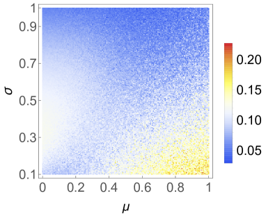
Figure 20: Absolute difference between the consensus resulting from Algorithm RepC when node one $1$ is under attack to share the a Gaussian noise with mean $\mu$ and standard deviation $\sigma$.

We can see from Fig. 20 that, in average, we obtain a small final consensus error. When $\mu$ is close to $1$ and $\sigma$ is close to $0.1$, the attacked node state value is close to what would be when in the non-attacked scenario ($x_{1}^{(0)}=1$) and it takes more time to be classified as an attacker by its neighbors, yielding a slightly larger final consensus error.

4 Conclusions

In this work, we presented a reputation-based consensus algorithm (RepC) for discrete-time synchronous and asynchronous communications in a possibly dynamic networks of agents. By assigning a reputation value to each neighbor, an agent may discard information from neighbors presenting an abnormal behavior.

Algorithm RepC converges with exponential rate and it has polynomial time complexity. More specifically, for a network of agents, if we run $i\in\mathbb{N}$ iterations of RepC, we incur in $\mathcal{O}(l^{2}i)$ time complexity, where $l$ is the greatest number of neighbors a node has in that network. For attacks with certain properties, we proved that the algorithm does not produce false positives. For other types of attacks, we illustrate the behavior of the proposed algorithm, which also worked as envisaged.

Future work directions include extending the algorithm for continuous-time consensus and to introduce the reputation idea for other types of consensus algorithms. Furthermore, an important additional theoretical property to prove (even if only for some sorts of attacks) is whether or not RepC may cause an agent to wrongly classify a neighbor as attacked, i.e., if there are false negatives.

References

- [AR07] P. Alriksson and A. Rantzer. Experimental evaluation of a distributed kalman filter algorithm. In 46th IEEE Conference on Decision and Control (CDC), pages 5499–5504, Dec 2007.
- [ASS11] D. Antunes, D. Silvestre, and C. Silvestre. Average consensus and gossip algorithms in networks with stochastic asymmetric communications. In 50th IEEE Conference on Decision and Control and European Control Conference, pages 2088–2093, Dec 2011.
- [BGPS06] Stephen Boyd, Arpita Ghosh, Balaji Prabhakar, and Devavrat Shah. Randomized gossip algorithms. IEEE transactions on information theory, 52(6):2508–2530, 2006.
- [CI12] Kai Cai and Hideaki Ishii. Average consensus on general strongly connected digraphs. Automatica, 48(11):2750–2761, 2012.
- [CKM18] Y. Chen, S. Kar, and J. M. F. Moura. Attack resilient distributed estimation: A consensus+innovations approach. In American Control Conference (ACC), pages 1015–1020, June 2018.
- [CLCD07] Mung Chiang, Steven H Low, A Robert Calderbank, and John C Doyle. Layering as optimization decomposition: A mathematical theory of network architectures. Proceedings of the IEEE, 95(1):255–312, 2007.
- [CMB06] Jorge Cortés, Sonia Martínez, and Francesco Bullo. Robust rendezvous for mobile autonomous agents via proximity graphs in arbitrary dimensions. IEEE Transactions on Automatic Control, 51(8):1289–1298, 2006.
- [DI15] Seyed Mehran Dibaji and Hideaki Ishii. Consensus of second-order multi-agent systems in the presence of locally bounded faults. Systems & Control Letters, 79:23–29, 2015.
- [DIT17] Seyed Mehran Dibaji, Hideaki Ishii, and Roberto Tempo. Resilient randomized quantized consensus. IEEE Transactions on Automatic Control, 2017.
- [DSI19] Seyed Mehran Dibaji, Mostafa Safi, and Hideaki Ishii. Resilient distributed averaging. In 2019 American Control Conference (ACC), pages 96–101. IEEE, 2019.
- [HA15a] A. Haseltalab and M. Akar. Approximate byzantine consensus in faulty asynchronous networks. In American Control Conference (ACC), pages 1591–1596, July 2015.
- [HA15b] A. Haseltalab and M. Akar. Convergence rate analysis of a fault-tolerant distributed consensus algorithm. In 54th IEEE Conference on Decision and Control (CDC), pages 5111–5116, Dec 2015.
- [HBC15] Ferry Hendrikx, Kris Bubendorfer, and Ryan Chard. Reputation systems: A survey and taxonomy. Journal of Parallel and Distributed Computing, 75:184–197, 2015.
- [JIB07] Audun Jøsang, Roslan Ismail, and Colin Boyd. A survey of trust and reputation systems for online service provision. Decision support systems, 43(2):618–644, 2007.
- [JKJJ08] B. Johansson, T. Keviczky, M. Johansson, and K. H. Johansson. Subgradient methods and consensus algorithms for solving convex optimization problems. In 47th IEEE Conference on Decision and Control (CDC), pages 4185–4190, Dec 2008.
- [JLM03] Ali Jadbabaie, Jie Lin, and A Stephen Morse. Coordination of groups of mobile autonomous agents using nearest neighbor rules. IEEE Transactions on automatic control, 48(6):988–1001, 2003.
- [KDI18] Y. Kikuya, S. M. Dibaji, and H. Ishii. Fault tolerant clock synchronization over unreliable channels in wireless sensor networks. IEEE Transactions on Control of Network Systems, pages 1–1, 2018.
- [LXYHC12] Rong-Hua Li, Jeffery Xu Yu, Xin Huang, and Hong Cheng. Robust reputation-based ranking on bipartite rating networks. In Proceedings of the 2012 SIAM international conference on data mining, pages 612–623. SIAM, 2012.
- [ÖA18] Halil Yiğit Öksüz and Mehmet Akar. Distributed resilient consensus: a non-parametric approach. Transactions of the Institute of Measurement and Control, page 0142331218785673, 2018.
- [OS07] R. Olfati-Saber. Distributed kalman filtering for sensor networks. In 46th IEEE Conference on Decision and Control (CDC), pages 5492–5498, Dec 2007.
- [OSM04] Reza Olfati-Saber and Richard M Murray. Consensus problems in networks of agents with switching topology and time-delays. IEEE Transactions on automatic control, 49(9):1520–1533, 2004.
- [PSD02] Josep M Pujol, Ramon Sangüesa, and Jordi Delgado. Extracting reputation in multi agent systems by means of social network topology. In Proceedings of the first international joint conference on Autonomous agents and multiagent systems: part 1, pages 467–474. ACM, 2002.
- [RB05] Wei Ren and Randal W Beard. Consensus seeking in multiagent systems under dynamically changing interaction topologies. IEEE Transactions on automatic control, 50(5):655–661, 2005.
- [RB20] Guilherme Ramos and Ludovico Boratto. Reputation (in)dependence in ranking systems: Demographics influence over output disparities. In Proceedings of the 43rd International ACM SIGIR Conference on Research and Development in Information Retrieval, SIGIR ’20, page 2061–2064, 2020.
- [RSS20a] Guilherme Ramos, Daniel Silvestre, and Carlos Silvestre. A general discrete-time method to achieve resilience in consensus algorithms. In 2020 59th IEEE Conference on Decision and Control (CDC), pages 2702–2707, 2020.
- [RSS20b] Guilherme Ramos, Daniel Silvestre, and Carlos Silvestre. General resilient consensus algorithms. International Journal of Control, 0(0):1–15, 2020.
- [SG18] S. Sundaram and B. Gharesifard. Distributed optimization under adversarial nodes. IEEE Transactions on Automatic Control, pages 1–1, 2018.
- [SHS18a] D. Silvestre, J. Hespanha, and C. Silvestre. A pagerank algorithm based on asynchronous gauss-seidel iterations. In American Control Conference (ACC), pages 484–489, June 2018.
- [SHS18b] D. Silvestre, J. P. Hespanha, and C. Silvestre. Broadcast and gossip stochastic average consensus algorithms in directed topologies. IEEE Transactions on Control of Network Systems, pages 1–1, 2018.
- [SPS+17] D. Saldana, A. Prorok, S. Sundaram, M. F. M. Campos, and V. Kumar. Resilient consensus for time-varying networks of dynamic agents. In American Control Conference (ACC), pages 252–258, May 2017.
- [SRC+13] D. Silvestre, P. Rosa, R. Cunha, J. P. Hespanha, and C. Silvestre. Gossip average consensus in a byzantine environment using stochastic set-valued observers. In 52nd IEEE Conference on Decision and Control, pages 4373–4378, Dec 2013.
- [SRCK17a] João Saúde, Guilherme Ramos, Carlos Caleiro, and Soummya Kar. Reputation-based ranking systems and their resistance to bribery. In 2017 IEEE International Conference on Data Mining (ICDM), pages 1063–1068. IEEE, 2017.
- [SRCK17b] João Saúde, Guilherme Ramos, Carlos Caleiro, and Soummya Kar. Robust reputation-based ranking on multipartite rating networks. arXiv preprint arXiv:1705.00947, 2017.
- [SRHS14] D. Silvestre, P. Rosa, J. P. Hespanha, and C. Silvestre. Finite-time average consensus in a byzantine environment using set-valued observers. In American Control Conference, pages 3023–3028, June 2014.
- [SRHS17] Daniel Silvestre, Paulo Rosa, João P. Hespanha, and Carlos Silvestre. Stochastic and deterministic fault detection for randomized gossip algorithms. Automatica, 78:46 – 60, 2017.
- [Sun16] S. Sundaram. Ignoring extreme opinions in complex networks: The impact of heterogeneous thresholds. In 55th IEEE Conference on Decision and Control (CDC), pages 979–984, Dec 2016.
- [TBA86] J. Tsitsiklis, D. Bertsekas, and M. Athans. Distributed asynchronous deterministic and stochastic gradient optimization algorithms. IEEE Transactions on Automatic Control, 31(9):803–812, September 1986.
- [UP18] James Usevitch and Dimitra Panagou. Resilient leader-follower consensus to arbitrary reference values. In American Control Conference (ACC). IEEE, 2018.
- [YAM+17] C. Yu, B. D. O. Anderson, S. Mou, J. Liu, F. He, and A. S. Morse. Distributed averaging using periodic gossiping. IEEE Transactions on Automatic Control, 62(8):4282–4289, Aug 2017.
- [ZM10] Minghui Zhu and Sonia Martínez. Discrete-time dynamic average consensus. Automatica, 46(2):322–329, 2010.
- [ZNLY15] Chunsheng Zhu, Hasen Nicanfar, Victor CM Leung, and Laurence T Yang. An authenticated trust and reputation calculation and management system for cloud and sensor networks integration. IEEE Transactions on Information Forensics and Security, 10(1):118–131, 2015.