Tuning Gap in Corrugated Graphene with Spin Dependence

Jaouad El-hassouny^a, Ahmed Jellal^b,c and El Houssine Atmani^a

^aLaboratory of Condensed Matter Physics and Renewed Energy, FST Mohammedia
Hassan II University, Casablanca, Morocco

^bLaboratory of Theoretical Physics, Faculty of Sciences, Chouaïb Doukkali University,

PO Box 20, 24000 El Jadida, Morocco

^cCanadian Quantum Research Center, 204-3002 32 Ave Vernon,
BC V1T 2L7, Canada

We study transmission in a system consisting of a curved graphene surface as an arc (ripple) of circle connected to two flat graphene sheets on the left and right sides. We introduce a mass term in the curved part and study the effect of a generated band gap in spectrum on transport properties for spin-up/-down. The tunneling analysis allows us to find all transmission and reflections channels in terms of the band gap. This later acts by decreasing the transmissions with spin-up/-down but increasing those with spin opposite, which exhibit different behaviors. We find resonances appearing in reflection with the same spin, thus backscattering with a spin-up/-down is not null in ripple. ome spatial shifts for the total conduction are observed in our model and the magnitudes of these shifts can be efficiently controlled by adjusting the band gap. This high order tunability of the tunneling effect can be used to design highly accurate devices based on graphene.

PACS numbers: 72.25.-b, 71.70.Ej, 73.23.Ad

Keywords: Graphene, ripple, mass term, spin transmission and reflection, conductance

1 Introduction

Graphene is an hexagonal rearrangement of carbon atoms [1, 2] and actually remains among the amazing two-dimensional systems discovered recently in material science. This because it exhibits interesting properties ranging from a linear dispersion relation to Klein tunneling paradox [3, 4]. In addition, the band structures in graphene are described by a low energy effective theory similar to the massless Dirac-Weyl fermions [5, 6]. Graphene possesses an exceptionally high mobility of the charge carriers. On the other hand, graphene stimulated the researchers to look for other two-dimensional materials. As a consequence, a great number with intriguing properties have been reported, covering metals, semiconductors, and insulators [7, 8, 9, 10, 11].

However, the inability to control such mobility is of paramount concern in nanoelectronics. This is due to the lack of band gap in its energy spectrum, which means that electric current in graphene cannot be completely shut off. Such characteristic makes graphene unsuitable for the development of many electronic devices and essentially reduces its applicability industrial and technological. Then, it is necessary to open a finite gap in the energy dispersions at $K$ point, which can be achieved by various experimental mechanisms. Indeed, an energy gap can be opened by deposing graphene sheet on a substrate. Indeed, a gap of 0.26 eV is induced in graphene by using silicon carbide (SiC) as substrate [12]. Also a gap of the order of 30 meV is produced by considering the hexagonal boron nitride (hBN) [13, 14]. The doping with boron [15, 16] or nitrogen [17] atoms can allow for opening and controlling an energy gap as well. As another alternative method one may use the strain engineering to realize an opened gap in graphene [18, 19, 20].

In recent years it has become evident that the physical properties of graphene can be changed by manipulating it in an external way to control its conductivity. Among the various mechanisms that may affect the carrier mobility, the diffusion that could be induced by ripple [21] appears to be the most natural since graphene sheets are naturally corrugated due to stress. It was shown that the amplitude and orientation of the unidirectional ripples can be controlled by a change in the components of an applied strain [22]. Several works discussed how to introduce ripples in graphene sheets in a controlled manner, and how to use such ripples [23, 24, 25, 26, 27, 28, 29]. Additionally, ripples can be created and controlled in suspended graphene, including heat treatment [28] and placing graphene in a specially prepared substrate. This is because the curvature of the surface affects the $\pi$ orbitals which determine the electronic properties of graphene. Ripples are distortions of the planar structure of the graphene, leading to measured charge mobilities much lower than theoretically predicted [30, 31].

The fundamental objective of this article is to extend the analysis in [32, 33] to a case when the corrugated graphene is subjected to an external delta deviation in mass term, which generates a band gap in the energy spectrum. We will attempt to answer how the added offset could be used to create a high efficiency polarized spin current in a corrugated graphene system. Then in the first stage, we derive the energy spectrum and use the transfer matrix to analytically obtain the full transmission and reflection channels. We show that the creation of band energy acts by decreasing the transmissions with spin-up/-down but increasing with spin opposite, which exhibit different behaviors. We find resonances appearing in reflection with the same spin, thus backscattering with a spin-up/-down is not null in ripple. Consequently, starting from some critical values of the band gap it appears that the spin filter get affected, which is resulted in reduction of the channels. Furthermore, we show that the total conductance get affected by the band gap in contrary to the case of null gap [32, 33]. Generally, we show that the presence of a band gap can be used as a key tool to control the transport properties of our system.

The present paper is organized as follow. In section 2, we formulate our problem and determine the solutions of energy spectrum in curved and flat regions of graphene. In section 3, we apply the boundary conditions at two interfaces to generate a transfer matrix allowing us to derive the transmission and reflection channels. Subsequently, we obtain the total conductance using four transmission channels indexed by spin-up/-down. We numerically study our results and provide different discussions as well as analysis in section 4. Finally, we conclude our work.

2 Model setting

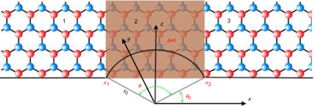
We study the scattering problem through a graphene involving in the central region a curved surface as arc of circle with radius $r_{0}$, or a ripple, and mass term $\Delta$. In fact, we consider corrugated graphene as depicted in Figure 1 with region 1: $x\in]-\infty,x_{1}]$, region 3: $x\in[x_{2},\infty[$ and region 2: $x\in[x_{1},x_{2}]$, such that $x_{1}=-x_{2}=-r_{0}\cos\theta_{0}$. In neglecting edge effects we assume that ${W}\gg{L},$ (${W}$ and ${L}$ being the width along $y$- and length along $x$-directions of graphene, respectively) and the ballistic electrons are injected to ripple in the perpendicular direction, i.e. $k_{y}=0$.

Figure 1: Graphene system composed of there regions such that the medium one is an arc (ripple) of radius $r_{0}$ involving a mass term $\Delta$.

The present system can be described in the basis $(F_{A\uparrow},F_{A\downarrow},F_{B\uparrow},F_{B\downarrow})$ of two sub-lattices $(A,B)$ by the Hamiltonian spin dependent

$$H=\begin{pmatrix}0&{D}\\ {D}^{\dagger}&0\end{pmatrix}$$ (1)

such that the operators are given by

$${D}=\gamma\left({p}_{x}-i{p}_{y}\right)\mathbb{I}+i\frac{\delta\gamma^{\prime}}{4r_{0}}{\sigma_{r}}-\frac{2\delta\gamma p}{r_{0}}{\sigma_{y}}+\Delta{\sigma_{\theta}}$$ (2)

$${D}^{\dagger}=\gamma\left({p}_{x}+i{p}_{y}\right)\mathbb{I}-i\frac{\delta\gamma^{\prime}}{4r_{0}}{\sigma_{r}}-\frac{2\delta\gamma p}{r_{0}}{\sigma_{y}}+\Delta{\sigma_{\theta}}$$ (3)

where ${p}_{x}=-\frac{i\hbar}{r_{0}}{\partial}_{\theta},{p}_{y}=-i\hbar{\partial}_{y}$, ${\sigma_{r}}={\sigma_{x}}\cos\theta-{\sigma_{z}}\sin\theta$, ${\sigma_{\theta}}=-{\sigma_{x}}\sin\theta-{\sigma_{z}}\cos\theta$ and ${\sigma}_{x,y,z}$ are Pauli matrices. The set of involved parameters is given by [34]

$$\gamma=-\frac{\sqrt{3}}{2}V_{pp}^{\pi}a=\gamma_{0}a,\qquad\gamma^{\prime}=\frac{\sqrt{3}}{2}\left(V_{pp}^{\sigma}-V_{pp}^{\pi}\right)a=\gamma_{1}a,\qquad p=\frac{1-3\gamma^{\prime}}{8\gamma}$$ (4)

with $V_{pp}^{\alpha}$ and $V_{pp}^{\pi}$ are the transfer integrals for $\sigma$ and $\pi$ orbitals, respectively. In the flat graphene, $a=$ $\sqrt{3}d\simeq 2.46\AA$ is the length of the primitive translation vector, with $d$ is the distance between atoms in the unit cell. As for the intrinsic source of the spin-orbit coupling $\delta$ we have

$$\delta=i\frac{\hbar}{4m_{e}^{2}c^{2}\epsilon_{\pi\sigma}}\left\langle x\left|\frac{\partial V}{\partial x}{p}_{y}-\frac{\partial V}{\partial y}{p}_{x}\right|y\right\rangle$$ (5)

with the atomic potential $V$ and $\epsilon_{\pi\sigma}=\epsilon_{2p}^{\pi}-\epsilon_{2p}^{\sigma}$, such that $\epsilon_{2p}^{\sigma}$ is the energy of $\sigma$ orbitals (localized between carbon atoms) and $\epsilon_{2p}^{\pi}$ is the energy of $\pi$ orbitals (directed perpendicular to the curved surface). In the next, for our numerical purpose it is convenient to choose $\gamma=6.39\ \mathrm{\SIUnitSymbolAngstrom}\ \mathrm{eV},\gamma^{\prime}=17.04\ \mathrm{\SIUnitSymbolAngstrom}\ \mathrm{eV},\delta=0.01$, $p=0.1$.

To simply diagonalize the Hamiltonian $H$ (1) we get rid of the $\theta$-dependence by making use of the unitarty transformation in terms of $\sigma_{y}$, which is

$${U}=\begin{pmatrix}e^{i\frac{\theta}{2}{\sigma}_{y}}&0\\ 0&e^{i\frac{\theta}{2}{\sigma}_{y}}\end{pmatrix}$$ (6)

and then it transforms (1) into the following

$$\mathcal{H}={U}{H}{U}^{-1}$$ (7)

giving rise to the Hamiltonian

$$\mathcal{H}=\begin{pmatrix}0&0&-\gamma\partial_{y}-\Delta-\mathrm{i}\frac{\gamma}{r_{0}}\partial_{\theta}&\mathrm{i}\left(\lambda_{y}+\lambda_{x}\right)\\ 0&0&\mathrm{i}\left(\lambda_{y}-\lambda_{x}\right)&-\gamma\partial_{y}+\Delta-\mathrm{i}\frac{\gamma}{r_{0}}\partial_{\theta}\\ \gamma\partial_{y}-\Delta-\mathrm{i}\frac{\gamma}{r_{0}}\partial_{\theta}&-\mathrm{i}\left(\lambda_{y}-\lambda_{x}\right)&0&0\\ -\mathrm{i}\left(\lambda_{y}+\lambda_{x}\right)&\gamma\partial_{y}+\Delta-\mathrm{i}\frac{\gamma}{r_{0}}\partial_{\theta}&0&0\end{pmatrix}$$ (8)

where we have set $\hbar=1$. One can define the total angular momentum by

$${J}_{y}=\begin{pmatrix}-\mathrm{i}\partial_{\theta}&\frac{-\mathrm{i}}{2}&0&0\\ \frac{\mathrm{i}}{2}&-\mathrm{i}\partial_{\theta}&0&0\\ 0&0&-\mathrm{i}\partial_{\theta}&\frac{-\mathrm{i}}{2}\\ 0&0&\frac{\mathrm{i}}{2}&-\mathrm{i}\partial_{\theta}\end{pmatrix}$$ (9)

which transforms as $\mathcal{J}_{y}={U}{J}_{y}{U}^{-1}$ and

$$\mathcal{J}_{y}=\begin{pmatrix}-\mathrm{i}\partial_{\theta}&0&0&0\\ 0&-\mathrm{i}\partial_{\theta}&0&0\\ 0&0&-\mathrm{i}\partial_{\theta}&0\\ 0&0&0&-\mathrm{i}\partial_{\theta}\end{pmatrix}.$$ (10)

Now based on the fact that $\left[\mathcal{H},\mathcal{J}_{y}\right]=0$ holds, we can use the separability of eigenspinors and then write $\mathcal{F}(\theta,y)$ as

$$\mathcal{F}(\theta,y)=e^{\mathrm{i}m\theta}e^{\mathrm{i}k_{y}y}\begin{pmatrix}A\\ B\\ C\\ D\end{pmatrix}$$ (11)

where $e^{\mathrm{i}m\theta}$ are eigensates of $\mathcal{J}_{y}$ associated to the eigenvalues $m=\pm\frac{1}{2},\pm\frac{3}{2},\cdots$. By injecting (8) and (11) into the eigenvalue equation $\mathcal{H}\mathcal{F}(\theta,y)=E\mathcal{F}(\theta,y)$ we find

$$\begin{pmatrix}0&0&t_{m}-\Delta-\mathrm{i}t_{y}&\mathrm{i}\left(\lambda_{y}+\lambda_{x}\right)\\ 0&0&\mathrm{i}\left(\lambda_{y}-\lambda_{x}\right)&t_{m}+\Delta-\mathrm{i}t_{y}\\ t_{m}-\Delta+\mathrm{i}t_{y}&-\mathrm{i}\left(\lambda_{y}-\lambda_{x}\right)&0&0\\ -\mathrm{i}\left(\lambda_{y}+\lambda_{x}\right)&t_{m}+\Delta+\mathrm{i}t_{y}&0&0\end{pmatrix}\begin{pmatrix}A\\ B\\ C\\ D\end{pmatrix}=E\begin{pmatrix}A\\ B\\ C\\ D\end{pmatrix}$$ (12)

which allows to end up with four bands $E_{s}^{s^{\prime}}$ for the Hamiltonian $H$

$$E_{s}^{s^{\prime}}=s^{\prime}\sqrt{\Delta^{2}+t_{m}^{2}+t_{y}^{2}+\lambda_{x}^{2}+\lambda_{y}^{2}+2s\sqrt{t_{m}^{2}\left(\Delta^{2}+\lambda_{x}^{2}\right)+\left(\Delta^{2}+t_{y}^{2}+\lambda_{x}^{2}\right)\lambda_{y}^{2}}}$$ (13)

where $s,s^{\prime}=\pm$ and we have set $t_{m}=\frac{\gamma}{r_{0}}m$, $t_{y}=\gamma k_{y}$, $\lambda_{x}=\frac{\gamma}{2r_{0}}(1+4\delta p)$, $\lambda_{y}=\frac{\delta\gamma^{\prime}}{4r_{0}}$. Note that for normal incidence, i.e. $k_{y}=0,$ (13) reduces to

$$E_{s}^{s^{\prime}}=s^{\prime}\sqrt{t_{m}^{2}+\lambda_{y}^{2}}+s\sqrt{\Delta^{2}+\lambda_{x}^{2}}$$ (14)

which can be used to index the eigenvalues of $\mathcal{J}_{y}$ as

$$m_{s}^{s^{\prime}}=s^{\prime}\frac{r_{0}}{\gamma}\sqrt{\left(E_{s}^{s^{\prime}}-s\sqrt{\Delta^{2}+\lambda_{x}^{2}}\right)^{2}-\lambda_{y}^{2}}$$ (15)

a result that will be employed in the boundary conditions to determine the transmission and reflections coefficients.

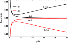
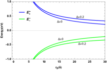
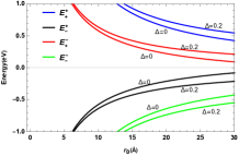
To show the effect of the mass term $\Delta$, we plot the four bands (14) as a function of the radius of the curvature $r_{0}$ in Figure 2 for $\delta=0.01,p=0.1$. For $m=\frac{1}{2}$ in left panel, we observe that at $r_{0}=0$, the energies $E_{+}^{-}$ and $E_{-}^{+}$ have an infinite value. At $r_{0}\neq 0$, the difference between $E_{+}^{-}$ and $E_{-}^{+}$ is very small for $\Delta=0$ but this difference increases with $\Delta=0.2$. In the middle panel, at $\Delta=0$, the difference between the energy $E_{+}^{+}$ and $E_{-}^{-}$ is greater than that of the left panel. On the other hand, at $\Delta=0.2$, this difference increases. For $m=\frac{3}{2}$ in right panel, the shape of the curve of the four energies changes in the neighborhood of the interval $[0,5]$ for the radius $r_{0}$. At $\Delta=0.2$, the difference between $E_{+}^{-}$ and $E_{-}^{+}$ is greater than at $\Delta=0$, as well as for $E_{+}^{+}$ and $E_{-}^{-}$. This shows that the introduction of the gap $\Delta$ is very necessary to control the differences between energies.

Figure 2: (color online) The four bands as a function of the radius $r_{0}$ for $\delta=0.01,p=0.1$ with $m=\frac{1}{2}$ (left and middle panels), $m=\frac{3}{2}$ (right panel). $E_{+}^{+}$ (blue), $E_{-}^{+}$ (black), $E_{+}^{-}$ (red), $E_{-}^{-}$ (green).

To completely determine the solutions of energy spectrum, we solve (12) to end up with the quantities

$$A_{s,s^{\prime}}(m)=s^{\prime}\frac{\lambda_{x}\sqrt{t_{m}^{2}+\lambda_{y}^{2}}+s\lambda_{y}\sqrt{\Delta^{2}+\lambda_{x}^{2}}}{\lambda_{x}t_{m}-\lambda_{y}\Delta}$$ (16)

$$B_{s,s^{\prime}}(m)=-is^{\prime}\frac{\Delta\sqrt{t_{m}^{2}+\lambda_{y}^{2}}+st_{m}\sqrt{\Delta^{2}+\lambda_{x}^{2}}}{\lambda_{x}t_{m}-\lambda_{y}\Delta}$$ (17)

$$C=1$$ (18)

$$D_{s}(m)=-i\frac{t_{m}\Delta+\lambda_{y}\lambda_{x}+s\sqrt{(t_{m}^{2}+\lambda_{y}^{2})(\Delta^{2}+\lambda_{x}^{2})}}{\lambda_{x}t_{m}-\lambda_{y}\Delta}$$ (19)

and according to (15) we have $m=m_{s}^{s^{\prime}}$. Consequently the eigenspinors associated to four bands (14) take the form

$$\Psi_{2}^{s,s^{\prime}}(\theta,m)=\begin{pmatrix}\cos\frac{\theta}{2}A_{s,s^{\prime}}(m)-\sin\frac{\theta}{2}B_{s,s^{\prime}}(m)\\ \sin\frac{\theta}{2}A_{s,s^{\prime}}(m)+\cos\frac{\theta}{2}B_{s,s^{\prime}}(m)\\ \cos\frac{\theta}{2}-\sin\frac{\theta}{2}D_{s}(m)\\ \sin\frac{\theta}{2}+\cos\frac{\theta}{2}D_{s}(m)\end{pmatrix}e^{im\theta}.$$ (20)

As a result, in region 2 the wave function can be written as a superposition of all solutions for a curved surface in the form

$$\Psi_{2}(\theta)=a_{+}\Psi_{2}^{+}\left(\theta,m_{+}^{+}\right)+b_{+}\Psi_{2}^{+}\left(\theta,m_{+}^{-}\right)+a_{-}\Psi_{2}^{-}\left(\theta,m_{-}^{+}\right)+b_{-}\Psi_{2}^{-}\left(\theta,m_{-}^{-}\right)$$ (21)

$a_{\pm}$ and $b_{\pm},$ denote the coefficients of the linear combination.

As for flat graphene (refers to regions 1 and 3), one can solve the eigenvalue equation to derive the two band energy at $k_{y}=0$

$$E=\pm\gamma|k|$$ (22)

and due to the energy conservation we have the relation $E=E^{s^{\prime}}_{s}$. The associated eigenspinors are given by

$$\Psi_{1(3)}^{\tau}(x,k)=\frac{1}{2}\begin{pmatrix}\text{sign}(k)\\ \text{sign}(k)\ i\tau\\ 1\\ i\tau\end{pmatrix}e^{ikx}$$ (23)

where $\tau=\pm$, $k=k_{x}$ and $\text{sign}(k)=\pm$ refers to conductance and valence bands, respectively. As a result the eigenspinors can be written a superposition of all possible solutions for flat graphene, such as in region 1

$$\Psi_{1}(x,k)=\alpha\Psi_{1}^{+}(x,k)+\beta\Psi_{1}^{-}(x,k)+r_{\uparrow}^{\xi}\Psi_{1}^{+}(x,-k)+r_{\downarrow}^{\xi}\Psi_{1}^{-}(x,-k)$$ (24)

and in region 3

$$\Psi_{3}(x,k)=t_{\uparrow}^{\xi}\Psi_{3}^{+}(x,k)+t_{\downarrow}^{\xi}\Psi_{3}^{-}(x,k)$$ (25)

with $\alpha=0,\beta=1$ for spin-down (${\xi}={\downarrow}$) and $\alpha=1,\beta=0$ for spin-up (${\xi}={\uparrow}$) polarizations. The coefficients $r_{\uparrow}^{\xi},r_{\downarrow}^{\xi},t_{\uparrow}^{\xi},t_{\downarrow}^{\xi}$ denote eight channels of reflection and transmission. In the next, we will implement the above results to study some features of the present system. More precisely, we analyze the tunneling effect and discuss the influence of energy gap on transmission and reflection channels.

3 Transport properties

To determine the transmission and reflection amplitudes, we consider the continuity of eigenspinors at the two interfaces $(x_{1}=-r_{0}\cos\theta_{0},\theta_{1}=\pi+\theta_{0})$ and $(x_{2}=r_{0}\cos\theta_{0},\theta_{2}=2\pi-\theta_{0})$. This process yields the set of equations

$$\alpha\Psi_{1}^{+}(x_{1},k)+\beta\Psi_{1}^{-}(x_{1},k)+r_{\uparrow}^{\xi}\Psi_{1}^{+}(x_{1},-k)+r_{\downarrow}^{\xi}\Psi_{1}^{-}(x_{1},-k)=$$

$$a_{+}\Psi_{2}^{+}\left(\theta_{1},m_{+}^{+}\right)+b_{+}\Psi_{2}^{+}\left(\theta_{1},m_{+}^{-}\right)+a_{-}\Psi_{2}^{-}\left(\theta_{1},m_{-}^{+}\right)+b_{-}\Psi_{2}^{-}\left(\theta_{1},m_{-}^{-}\right)$$ (26)

$$a_{+}\Psi_{2}^{+}\left(\theta_{2},m_{+}^{+}\right)+b_{+}\Psi_{2}^{+}\left(\theta_{2},m_{+}^{-}\right)+a_{-}\Psi_{2}^{-}\left(\theta_{2},m_{-}^{+}\right)+b_{-}\Psi_{2}^{-}\left(\theta_{2},m_{-}^{-}\right)=$$

$$t_{\uparrow}^{\xi}\Psi_{1}^{+}(x_{2},k)+t_{\downarrow}^{\xi}\Psi_{1}^{-}(x_{2},k)$$ (27)

where $\xi=\downarrow,\uparrow$ refers to spin-up/-down. Now by eliminating the parameters $a_{\pm}$ and $b_{\pm},$ we derive the relation

$$\begin{pmatrix}\alpha\\ \beta\\ r_{\uparrow}^{\xi}\\ r_{\downarrow}^{\xi}\end{pmatrix}=M_{0}^{-1}M\left(\frac{3\pi-\phi}{2}\right){D}(-\phi)M^{-1}\left(\frac{3\pi+\phi}{2}\right)M_{0}\begin{pmatrix}t_{\uparrow}^{\xi}\\ t_{\downarrow}^{\xi}\\ 0\\ 0\end{pmatrix}$$ (28)

and we have introduced the angle $\phi=\pi-2\theta_{0}.$ Note that for moving electrons in (28) the configuration $\alpha=0,\beta=1$ is spin down polarization (${\xi}={\downarrow}$), while $\alpha=1,\beta=0$ for spin up one (${\xi}={\uparrow}$). The involved matrix are given by

$$M_{0}=\begin{pmatrix}1&1&-1&-1\\ i&-i&-i&i\\ 1&1&1&1\\ i&-i&i&-i\end{pmatrix},\qquad{D}(\phi)=\begin{pmatrix}e^{im_{+}\phi}&0&0&0\\ 0&e^{im_{-}\phi}&0&0\\ 0&0&e^{-im_{+}\phi}&0\\ 0&0&0&e^{-im_{-}\phi}\end{pmatrix}$$ (29)

and we have

$$M\left(\frac{3\pi+\phi}{2}\right)=\Lambda M_{A}$$ (30)

such that $\Lambda$ is

$$\Lambda=\begin{pmatrix}\cos\frac{3\pi+\phi}{4}&-\sin\frac{3\pi+\phi}{4}&0&0\\ \sin\frac{3\pi+\phi}{4}&\cos\frac{3\pi+\phi}{4}&0&0\\ 0&0&\cos\frac{3\pi+\phi}{4}&-\sin\frac{3\pi+\phi}{4}\\ 0&0&\sin\frac{3\pi+\phi}{4}&\cos\frac{3\pi+\phi}{4}\end{pmatrix}$$ (31)

as well as $M_{A}$ reads as

$$M_{A}=\begin{pmatrix}A_{+,s^{\prime}}(m_{+})&A_{-,s^{\prime}}(m_{-})&A_{+,s^{\prime}}(-m_{+})&A_{-s^{\prime}}(-m_{-})\\ B_{+,s^{\prime}}(m_{+})&B_{-,s^{\prime}}(m_{-})&B_{+,s^{\prime}}(-m_{+})&B_{-,s^{\prime}}(-m_{-})\\ 1&1&1&1\\ D_{+}(m_{+})&D_{-}(m_{-})&D_{+}(-m_{+})&D_{-}(-m_{-})\\ \end{pmatrix}.$$ (32)

where $s^{\prime}=+1$ for $|E|\geq\sqrt{\lambda_{x}^{2}+\Delta^{2}}$ and $s^{\prime}=-1$ for $|E|<\sqrt{\lambda_{x}^{2}+\Delta^{2}}$. Then from the above analysis we deduce the transfer matrix

$$\mathcal{M}=M_{0}^{-1}\left(\Lambda M_{A}\right){D}(-\phi)\left(\Lambda M_{A}\right)^{-1}M_{0}=\left(\mathcal{M}_{ij}\right)$$ (33)

with $i,j=1,2,3,4$. After a lengthy and straightforward algebra, we end up with the transmission and reflection amplitudes for spin-up

$$t_{\uparrow}^{\uparrow}=\frac{\mathcal{M}_{22}}{\mathcal{M}_{22}\mathcal{M}_{11}-\mathcal{M}_{21}\mathcal{M}_{12}},\qquad t_{\downarrow}^{\uparrow}=-\frac{\mathcal{M}_{21}}{\mathcal{M}_{22}\mathcal{M}_{11}-\mathcal{M}_{21}\mathcal{M}_{12}}$$ (34)

$$r_{\uparrow}^{\uparrow}=\mathcal{M}_{31}t_{\uparrow}^{\uparrow}+\mathcal{M}_{32}t_{\downarrow}^{\uparrow},\qquad\qquad\ \ r_{\downarrow}^{\uparrow}=\mathcal{M}_{41}t_{\uparrow}^{\uparrow}+\mathcal{M}_{42}t_{\downarrow}^{\uparrow}$$ (35)

as well as for spin-down

$$t_{\downarrow}^{\downarrow}=\frac{\mathcal{M}_{11}}{\mathcal{M}_{22}\mathcal{M}_{11}-\mathcal{M}_{21}\mathcal{M}_{12}},\qquad t_{\uparrow}^{\downarrow}=-\frac{\mathcal{M}_{12}}{\mathcal{M}_{22}\mathcal{M}_{11}-\mathcal{M}_{21}\mathcal{M}_{12}}$$ (36)

$$r_{\uparrow}^{\downarrow}=\mathcal{M}_{31}t_{\uparrow}^{\downarrow}+\mathcal{M}_{32}t_{\downarrow}^{\downarrow},\qquad\qquad\ \ r_{\downarrow}^{\downarrow}=\mathcal{M}_{41}t_{\uparrow}^{\downarrow}+\mathcal{M}_{42}t_{\downarrow}^{\downarrow}.$$ (37)

From (34) and (36) we can derive the relation

$$t_{\uparrow}^{\uparrow}=\frac{\mathcal{M}_{22}}{\mathcal{M}_{21}}t_{\downarrow}^{\uparrow}=\frac{\mathcal{M}_{22}}{\mathcal{M}_{11}}t_{\downarrow}^{\downarrow}=\frac{\mathcal{M}_{22}}{\mathcal{M}_{12}}t^{\downarrow}_{\uparrow}.$$ (38)

Since the wave vector of input is the same as of output, then the associated transmission and reflection probabilities take the forms

$$T_{\uparrow}^{\uparrow}=|t_{\uparrow}^{\uparrow}|^{2},\qquad\ T_{\downarrow}^{\downarrow}=|t_{\downarrow}^{\downarrow}|^{2},\qquad T_{\uparrow}^{\downarrow}=|t_{\uparrow}^{\downarrow}|^{2},\qquad T_{\downarrow}^{\uparrow}=|t_{\downarrow}^{\uparrow}|^{2}$$ (39)

$$R_{\uparrow}^{\uparrow}=|r_{\uparrow}^{\uparrow}|^{2},\qquad R_{\downarrow}^{\downarrow}=|r_{\downarrow}^{\downarrow}|^{2},\qquad R_{\uparrow}^{\downarrow}=|r_{\uparrow}^{\downarrow}|^{2},\qquad R_{\downarrow}^{\uparrow}=|r_{\downarrow}^{\uparrow}|^{2}.$$ (40)

The conductance associated to our system can be obtained via the Landauer-Büttiker formula [35, 36, 37] at zero temperature. It was shown that the conductance of one propagating channel can easily be generalized to any number of incoming and outgoing channels [38, 39, 40]. There are different conductances resulted from the transmittances between states of definite momentum and spin projection at the contacts [41]. Consequently, the total conductance in the linear response regime is given by summing over all the transmission channels

$$G=\frac{e^{2}}{h}\left(T_{\uparrow}^{\uparrow}+T_{\downarrow}^{\downarrow}+T_{\uparrow}^{\downarrow}+T_{\downarrow}^{\uparrow}\right)=\frac{e^{2}}{h}\sum_{p,q=\xi}T_{p}^{q}.$$ (41)

These results will numerically be analyzed under suitable choices of the physics parameters involved in our system. This study will allow us to show the role that could play the energy gap to modify the electronic properties of our system.

4 Numerical results

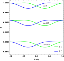
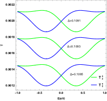
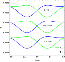
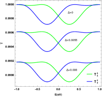
We study the tunneling properties of our system under suitable choices of the involved parameters ($r_{0},\Delta,\phi$) at normal incidence, i.e. $k_{y}=0$. Indeed, Figure 3 shows the transmissions $T_{\uparrow}^{\uparrow}$ (blue) and $T_{\downarrow}^{\downarrow}$ (green) with same spin as a function of the incident energy $E$ for different values of the band gap with the angle $\phi=\frac{4\pi}{5}$. As a first result we notice that the transmission preserves the symmetry because we have $T_{\uparrow}^{\uparrow}(E)=T_{\downarrow}^{\downarrow}(-E)$ for all $E$. Now in the upper panels we choose the radius of curvature $r_{0}=10$ $\mathrm{\SIUnitSymbolAngstrom}$, then for $\Delta=0$ one observes that the transmission behavior varies slowly closed to the unit. As for $\Delta\neq 0$, according to Figures 3a,3b,3c we notice that the transmission decreases as long as $\Delta$ increases and starts to move away from the unit. Furthermore, the increase of $\Delta$ causes a delay in the energy interval where the transmission of the spin down becomes minimal at $E=\sqrt{\lambda_{x}^{2}+\Delta^{2}}$. The bottom panels are as before except that $r_{0}=12$ $\mathrm{\SIUnitSymbolAngstrom}$ and then Figures 3d,3e,3f tell us that the transmission decreases by increasing $\Delta$ while its symmetrical shape still the same.

(a)

(b)

(c)

(d)

(e)

(f)

Figure 3: (color online) The transmission probabilities $T_{\uparrow}^{\uparrow}$ (blue) and $T_{\downarrow}^{\downarrow}$ (green) at normal incidence as a function of the incident energy $E$ for different values of the band gap $\Delta$ with $\phi=\frac{4\pi}{5}$. The radius $r_{0}=10$ $\mathrm{\SIUnitSymbolAngstrom}$ for top panels and $r_{0}=12$ $\mathrm{\SIUnitSymbolAngstrom}$ for bottom panels.

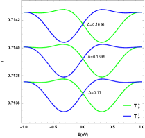
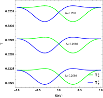
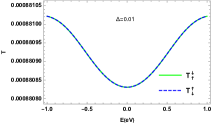
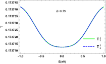
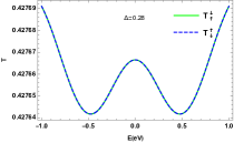
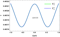
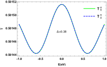
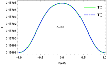
In Figure 4 we present the transmissions of the opposite spin $T^{\uparrow}_{\downarrow}$ (dashed blue) and $T^{\downarrow}_{\uparrow}$ (green) as a function of the incident energy $E$ for different values of the band gap $\Delta$ with the angle $\phi=\frac{4\pi}{5}$ and radius $r_{0}=10\ \mathrm{\SIUnitSymbolAngstrom}$. We emphasis that both transmissions always keep a symmetrical behavior such as the relation $T_{\uparrow}^{\downarrow}=T_{\downarrow}^{\uparrow}$ is satisfied. We start by noting that for $\Delta=0$ in Figure 4a both transmissions are almost null as obtained in [32]. However, for $\Delta\neq 0$ it is clear that the transmission increases progressively by oscillating under the increase of $\Delta$ as in particular for $\Delta=0.15$ eV in Figure 4b and $\Delta=0.28$ eV in 4c. Interestingly, for $\Delta=0.33$ eV one sees that the transmission can be approached by a sinusoidal function as depicted in Figure 4d but for $\Delta=0.38$ eV it oscillates differently according to Figure 4e with a remarkably change in its amplitudes and such manifestation is due of course to the presence of $\Delta$. Finally for $\Delta=0.6$ eV in Figure 4f, we notice that the transmission takes a characteristic form that has a Gaussian shape. As a result, we observe that the increase of $\Delta$ changes dramatically the transmission behavior. It is clearly seen that $\Delta$ affects all transmission channels and then can be used a controllable toy to adjust the tunneling properties toward a technological application.

(a)

(b)

(c)

(d)

(e)

(f)

Figure 4: (color online) The transmission probabilities $T^{\uparrow}_{\downarrow}$ (dashed blue) and $T^{\downarrow}_{\uparrow}$ (green) at normal incidence as a function of the incident energy $E$ for different values of band gap $\Delta$ with $\phi=\frac{4\pi}{5}$ and $r_{0}=10$ $\mathrm{\SIUnitSymbolAngstrom}.$

(a)

(b)

(c)

(d)

(e)

(f)

Figure 5: (color online) The reflection probabilities in the logarithmic scale ($R_{\uparrow}^{\uparrow}=R_{\downarrow}^{\downarrow}$, $R_{\downarrow}^{\uparrow}$, $R_{\uparrow}^{\downarrow}$) at normal incidence as a function of the incident energy $E$ for three values of the band gap $\Delta$ with $\phi=\frac{4\pi}{5}$ and $r_{0}=20\ \mathrm{\SIUnitSymbolAngstrom}$.

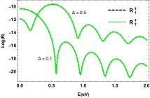
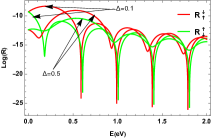
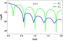
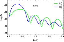
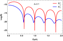
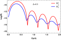
In Figure 5, we show the reflection probabilities in the logarithmic scale at normal incidence as a function of the incident energy $E$ for three values of the band gap $\Delta=(0.1,0.3,0.5)$ eV with the ripple angle $\phi=\frac{4\pi}{5}$ and radius $r_{0}=20$ $\mathrm{\SIUnitSymbolAngstrom}$. As an interesting consequence resulted from $\Delta\neq 0$ is the emergence of reflections with the same spin, namely $R_{\uparrow}^{\uparrow}=R_{\downarrow}^{\downarrow}\neq 0$, contrary to what obtained in [32] for gapless case ($\Delta=0$), see Figure 5a. This means that the Klein tunneling is not always satisfied with the presence of band gap. Figure 5b tells us that the reflections with opposite spin do not show the same behavior and consequently we have $R_{\uparrow}^{\downarrow}\neq R_{\downarrow}^{\uparrow}$. By comparing $R_{\uparrow}^{\uparrow}$ and $R_{\downarrow}^{\uparrow}$ we observe that the sharp peaks appearing in Figure 5c for $\Delta=0.1$ eV disappear in Figure 5d for $\Delta=0.3$ eV and then oscillations modes take place. We have the same conclusion for $R_{\uparrow}^{\uparrow}$ and $R^{\downarrow}_{\uparrow}$ in Figure 5e for $\Delta=0.1$ eV disappear in Figure 5f for $\Delta=0.3$ eV. Indeed, we observe that there are resonances in reflection with different amplitudes, which become important for $R_{\downarrow}^{\uparrow}$ and $R_{\uparrow}^{\downarrow}$ in particular for $\Delta=0.1$ eV as presented in Figure 5e. This behavior changes for $\Delta=0.3$ in Figure 5f where all reflection channels oscillate with large amplitudes and less resonances.

(a)

(b)

(c)

(d)

(e)

(f)

Figure 6: (color online) The transmission probabilities $T_{\uparrow}^{\uparrow}$ (blue dashed lines) and $T_{\downarrow}^{\downarrow}$ (green solid lines) at normal incidence as a function of the angle $\phi$ of ripple for different values of the band gap $\Delta$ with $E=0.6$ eV and $r_{0}=16$ $\mathrm{\SIUnitSymbolAngstrom}$.

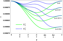
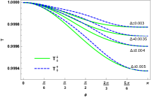
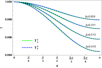
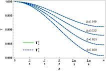
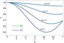
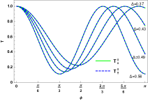
In Figure 6, we show the transmission probabilities with the same spin as a function of the ripple angle $\phi$ for different values of the band gap $\Delta$ with incident energy $E=0.6$ eV and radius $r_{0}=16\ \mathrm{\SIUnitSymbolAngstrom}$. Our results show a degradation of the capacity of spin filtering in our system due to $\Delta$. Consequently, in Figure 6a we observe that $T_{\uparrow}^{\uparrow}$ and $T_{\downarrow}^{\downarrow}$ have maximum values at $\phi=\pi$ for the case $\Delta=0$ as found in [32]. Now with the inclusion of mass term, we notice that both of transmissions decrease as long as $\phi$ increases but they approach to each others see Figures 6b,6c. By increasing $\Delta$, the transmissions coincide and show different behaviors in Figures 6d,6e. In particular, they show periodically oscillations as in Figure 6f and then one can theoretically approach them by sinusoidal functions. Consequently, we notice from a critical value of $\Delta$ the spin splitting is not longer maintained as clearly seen starting from Figure 6c, which reduces the spin degree of freedom by giving rise only to one transmission channel instead of two. Then, one can use $\Delta$ as a key ingredient to control the spin splitting in our system.

(a)

(b)

(c)

(d)

(e)

(f)

Figure 7: (color online) The transmission probabilities $T_{\uparrow}^{\uparrow}$ (blue dashed lines) and $T_{\downarrow}^{\downarrow}$ (green solid lines) at normal incidence as a function of the radius $r_{0}$ of ripple for different values of the band gap $\Delta$ with $E=0.6$ eV and $\phi=\frac{4\pi}{5}$.

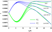
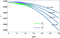
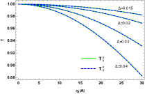
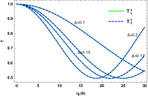
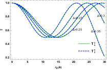
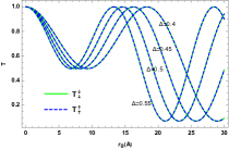
Figure 7 presents the transmission probabilities with the same spin versus the ripple radius for different values of the band gap $\Delta$ with incident energy $E=0.6$ eV and angle $\phi=\frac{4\pi}{5}$. Our results also show a degradation of the capacity of the spin filter due to $\Delta$. In Figure 7a with $\Delta$ in the range $[0,2\ 10^{-3}]$, we observe that $T_{\uparrow}^{\uparrow}$ (blue dashed lines) behaves differently compared to $T_{\downarrow}^{\downarrow}$ (green solid lines) when $r_{0}\in[0,16]$, but they approach to each other beyond. In Figure 7b, $T_{\uparrow}^{\uparrow}$ and $T_{\downarrow}^{\downarrow}$ mostly coincide and then after a critical value of $r_{0}$ they present the same behavior. In Figure 7c there is a perfect coincidence between $T_{\uparrow}^{\uparrow}$ and $T_{\downarrow}^{\downarrow}$. We observe some oscillations stared to appear from Figure 7d and become clear in Figure 7e. From $\Delta=0.55$, the behavior stabilizes and keeps the same minimum and maximum for any value of $\Delta$ as depicted in Figure 7f. Note that, in all case presented here we notice that both of transmissions decrease as long as $\Delta$ increases.

(a)

(b)

Figure 8: (color online) The conductance as a function of the incident energies $E$ for different values of the band gap $\Delta$ with $\phi=\frac{4\pi}{5}$ and $r_{0}=10\ \mathrm{\SIUnitSymbolAngstrom}$.

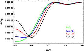
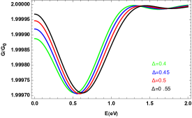
We show the conductance as a function of the incident energy in Figure 8 for different values of the band gap $\Delta$ with $r_{0}=10\ \mathrm{\SIUnitSymbolAngstrom}$ and $\phi=4\pi/5$. Our results show that the conductance changes its behavior on three different zones. According to Figure 8a, we can analyze the conductance behavior by considering three zones. Indeed, for the first zone $E\in[0,\sqrt{0.1+\Delta^{2}}]$ the conductance increases for $\Delta=0$, but it starts to decrease by increasing $\Delta$. Note that at $E=0$, there is a large spacing for each value of $\Delta$. For the second zone $E\in[\sqrt{0.1+\Delta^{2}},1.2]$ there are rapid increases in conductance but $\Delta$ acts by accelerating. In the third zone where $E$ is beyond the value $1.2$, the conductance becomes insensitive to any increase in energy $E$ and $\Delta$. This behavior is mainly changed in Figure 8b under the increase of $\Delta$ because in the zone $E\in[0,\sqrt{0.1+\Delta^{2}}]$ there is a rapid decrease in conductance for any $\Delta$ and reaches its maximum. In the second zone $E\in[\sqrt{0.1+\Delta^{2}},1.4]$ the conductance increases rapidly in order to stabilize beyond the value $E=1.4$. Finally, we notice that the increase in $\Delta$ causes some oscillations in the first and third zones.

(a)

(b)

Figure 9: (color online) The conductance as a function of the radius of ripple $r_{0}$ for different values of the band gap $\Delta$ with $\phi=\frac{4\pi}{5}$ and $E=0.6$ eV.

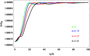
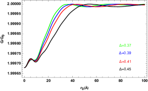
We show the conductance as a function of the ripple radius in Figure 9 for different values of the band gap $\Delta$ with $\phi=\frac{4\pi}{5}$ and $E=0.6$ eV. Our results show that the conductance changes its behavior by increasing $\Delta$. According to Figure 9a, one can analyze the conductance behavior by considering three different zones. Indeed, for the first zone $r_{0}\in[0,6]$ we have mostly the same increase of conductance what ever the value taken by $\Delta$. For the second zone $r_{0}\in[6,30]$ there are rapid increases in conductance but $\Delta$ acts on by speeding down. In the third zone where $r_{0}$ beyond the value 30, the conductance becomes insensible to any increase of radius and band gap. This behavior mostly changed in Figure 9b under the increase of $\Delta$ because in the first zone [0,9] we have a small oscillation with an amplitude and increases in the second zone where $r_{0}$ is in [9, 50] afterword it becomes constant in third zone.

(a)

(b)

Figure 10: (color online) The conductance as a function of the ripple angle $\phi$ for different values of the band gap $\Delta$ $r_{0}=16$ $\mathrm{\SIUnitSymbolAngstrom}$ and $E=0.6$ eV.

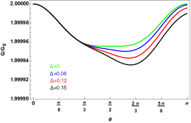
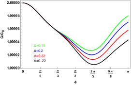
We show the conductance as a function of ripple angle $\phi$ in Figure 10 for different values of the band gap $\Delta$ with $r_{0}=16$ $\mathrm{\SIUnitSymbolAngstrom}$ and $E=0.6$ eV. Our results show that conductance completely changes its behavior. From Figure 10a, the behavior of conductance can be analyzed by considering three different areas. Indeed, for the first zone $\phi\in[0,\pi/3]$ the conductance coincides and decreases whatever the value taken by $\Delta$. For the second zone $\phi\in[\pi/3,2\pi/3]$ there are still decreases in conductance but there is a strong widening and reaching the minimum. In the third zone where $\phi$ is beyond the value 2$\pi/3$ the conductance becomes narrow and increases toward a maximum. In Figure 10b we observe that the only interesting change is the minimum become deeper compared to those seen in Figure 10a in addition to a reduction of the maximum amplitude.

5 Conclusion

We have studied the transport properties of electrons through the structure of corrugated graphene in the presence of mass term at normal incidence ($k_{y}=0$). By solving the Dirac equation and using the transfer matrix method, the four energy bands are obtained as a function of the opening band gap $\Delta$. Next, we have analyzed the transmissions and reflection channels together with the corresponding conductance. Indeed, we have shown that the presence of band gap $\Delta$ has a visible impact on electron scattering with different initial polarization.

Furthermore, our numerical results showed that there is a reflection of electrons with the same spin polarization of the incoming ones as a manifestation of $\Delta$. This situation does not exist in the absence of $\Delta$ as reported in [32, 33] and [42]. In the case under consideration, there is also the transmission for electrons with the opposite spin polarization, which gradually increase with the deviation of $\Delta$. We have also observed the decrease in transmission with same spin polarization. On the other hand, backscattering with the same polarization spin takes place because of the nonzero electron reflection.

Finally, we mention that the experiment realized by Kuemmeth et al. [43] demonstrated that in clean nanotubes the spin and orbital motion of electrons are coupled. We think that the technique employed in [43] can serve as a guide to experimentally reproduce our work. Our results could offer a way to engineer systems towards technological application. Indeed, may be our findings can find important implications for spin-based applications in carbon-based systems, providing a mechanism for all-electrical control of spins [44] and band gap.

References

- [1] K. S. Novoselov, A. K. Geim, S. V. Morozov, D. Jiang, M. I. Katsnelson, I. V. Grigorieva, S. V. Dubonos, and A. A. Firsov, Nature 438, 197 (2005).
- [2] Y. B. Zhang, Y. W. Tan, H. L. Störmer, and P. Kim, Nature 438, 201 (2005).
- [3] M. I. Katsnelson, Graphene: Carbon in Two Dimensions (Cambridge University Press, Cambridge, 2012).
- [4] L. E. F. Foa Torres, S. Roche, and J.-C. Charlier, Introduction to Graphene-Based Nanomaterials (Cambridge University Press, New York, 2014).
- [5] R. Saito, G. Dresselhaus, M. S. Dresselhaus, Physical Properties of Carbon Nanotubes (Imperial College Press, London, 1998).
- [6] A. H. Castro Neto, F. Guinea, N. M. R. Peres, K. S. Novoselov, A. K. Geim, Rev. Mod. Phys. 81, 109 (2009).
- [7] C. Tan, X. Cao, X.-J. Wu, Q. He, J. Yang, X. Zhang, J. Chen, W. Zhao, S. Han, G.-H. Nam, M. Sindoro, and H. Zhang, Chem. Rev. 117, 6225 (2017).
- [8] Jiajie Pei, Jiong Yang, Tanju Yildirim, Han Zhang, and Yuerui Lu, Adv. Mater. 31, 1706945 (2019).
- [9] Bo Guo, Quan-lan Xiao, Shi-hao Wang, and Han Zhang, Laser Photonics Rev. 13, 1800327 (2019).
- [10] abcd b Karim Khan, Ayesha Khan Tareen, Muhammad Aslam, Renheng Wang, Yupeng Zhang, Asif Mahmood, Zhengbiao Ouyang, Han Zhang, and Zhongyi Guo, J. Mater. Chem. C 8, 387 (2020).
- [11] Deepika Tyagi, Huide Wang, Weichun Huang, Lanping Hu, Yanfeng Tang, Zhinan Guo, Zhengbiao Ouyang, and Han Zhang, Nanoscale 12, 3535 (2020).
- [12] S. Y. Zhou, G.-H. Gweon, A. V. Fedorov, P. N. First, W. A. de Heer, D.-H. Lee, F. Guinea, A. H. Castro Neto, A. Lanzara, Nat. Matter 6 770 (2007).
- [13] P. San-Jose, A. Guti´errez-Rubio, M. Sturla, F. Guinea, Phys. Rev. B 90, 075428 (2014).
- [14] P. San-Jose, A. Gutiérrez-Rubio, M. Sturla, and F. Guinea, Phys. Rev. B 90, 115152 (2014).
- [15] J. Gebhardt, R. J. Koch, W. Zhao, O. Höfert, K. Gotterbarm, S. Mammadov, C. Papp, A. Görling, H.-P. Steinrück, and T. Seyller, Phys. Rev. B 87, 155437 (2013).
- [16] T. B. Martins, R. H. Miwa, A. J. R. da Silva, and A. Fazzio, Phys. Rev. Lett. 98, 196803 (2007).
- [17] H. Wang, T. Maiyalagan, and X. Wang, ACS Catalysis 2, 781 (2012).
- [18] V. M. Pereira and A. H. Castro Neto, Phys. Rev. Lett. 103, 046801 (2009).
- [19] T. Low, F. Guinea, and M. I. Katsnelson, Phys. Rev. B 83, 195436 (2011).
- [20] F. Guinea, Solid State Communications 152, 1437 (2012).
- [21] M. I. Katsnelson and A. K. Geim, Phil. Trans. R. Soc. A 366, 195 (2008).
- [22] J. A. Baimova, S. V. Dmitriev, K. Zhou, and A. V. Savin, Phys. Rev. B 86, 035427 (2012).
- [23] W. H. Duan, K. Gong, and Q. Wang, Carbon 49, 3107 (2011).
- [24] M. Neek-Amal and F. M. Peeters, Phys. Rev. B 82, 085432 (2010).
- [25] Z. F. Wang, Y. Zhang, and F. Liu, Phys. Rev. B 83, 041403(R) (2011).
- [26] F. Guinea, B. Horovitz, and P. Le Doussal, Solid State Commun. 149, 1140 (2009).
- [27] R. Miranda and A. L. Vazquez de Parga, Nat. Nanotechnol. 4, 549 (2009).
- [28] W. Bao, F. Miao, Z. Chen, H. Zhang, W. Jang, C. Dames, and C. N. Lau, Nat. Nanotechnol. 4, 562 (2009).
- [29] A. Fasolino, J. H. Los, and M. I. Katsnelson, Nat. Mater. 6, 858 (2007).
- [30] G. G. Naumis, S. Barraza-Lopez, M. Oliva-Leyva, and H. Terrones, Rep. Prog. Phys. 80, 096501 (2017).
- [31] P. Bøggild, D .M. Mackenzie, P. R. Whelan, D. H. Petersen, J. D. Buron, A. Zurutuza, J. Gallop, L. Hao, and P. U. Jepsen, 2D Mater. 4, 042003 (2017).
- [32] M. Pudlak, K. N. Pichugin, and R. G. Nazmitdinov, Phys. Rev. B 92, 205432 (2015).
- [33] M. Pudlak and R. Nazmitdinov, Physica E 118, 113846 (2020).
- [34] T. Ando, J. Phys. Soc. Jpn. 69, 1757 (2000).
- [35] M. Büttiker, Y. Imry, R. Landauer, and S. Pinhas, Phy. Rev. B 31, 6207 (1985).
- [36] R. Landauer, IBM J. Res. Dev. 1, 223 (1957).
- [37] J. Bundesmann, M.-H. Liu, I. Adagideli, and K. Richter, Phys. Rev. B 88, 195406 (2013).
- [38] Horacio M. Pastawski1 and Ernesto Medina, Revista Mexicana de Fisica 47S1, 1 (2001), cond-mat/0103219.
- [39] Horacio M. Pastawski, L. E. F. Foa Torres, and Ernesto Medina, Chemical Physics 281, 257 (2002).
- [40] Lucas Jonatan Fernández and Horacio Miguel Pastawski, Europhysics Letters 105, 17005 (2014).
- [41] Y. Imry and R. Landauer, Rev. Mod. Phys. 71, S306 (1999).
- [42] J. Smotlacha, M. Pudlak, and R. G. Nazmitdinov, J. Phys.: Conf. Ser. 1416, 012035 (2019).
- [43] F. Kuemmeth, S. Ilani, D. C. Ralph, and P. L. McEuen, Nature 452, 448 (2008).
- [44] K. C. Nowack, F. H. L. Koppens, Yu V. Nazarov, and L. M. K. Vandersypen, Science 318, 1430 (2007).