Collective Progress: Dynamics of Exit Waves

Abstract

We study a model of collective search by teams. Discoveries beget discoveries and correlated search results are governed by a Brownian path. Search results’ variation at any point—the search scope—is jointly controlled. Agents individually choose when to cease search and implement their best discovery. We characterize equilibrium and optimal policies. Search scope is constant and independent of search outcomes as long as no member leaves. It declines after departures. A simple drawdown stopping boundary governs each agent’s search termination. We show the emergence of endogenous exit waves, whereby possibly heterogeneous agents cease search all at once.

Keywords: Retrospective Search, Optimal Stopping, Collective Action, Exit Waves

JEL codes: C73, D81, D83, O35

1 Introduction

Discoveries are often made by teams. Advances in motor vehicles, communication devices, and pharmaceuticals frequently take place as joint ventures. Understanding collective progress is therefore vital for the analysis of innovation. Much of the literature on teamwork has focused on experimentation models, starting from the canonical work of Bolton and Harris (1999) and Keller et al. (2005). Those models center on teams’ efforts to ascertain whether one direction or project is superior to another. Nonetheless, many discovery processes follow a path of search. Building on past discoveries, teams come up with new ones. Furthermore, there is a richness of dynamics in collective efforts not captured in prior models—alliances tend to dissolve over time, with exiting members exploiting knowledge accrued during their collaborations.

This paper offers a new framework for studying collective progress based on a process of search. We identify how the breadth of search and decisions to terminate search vary with members’ characteristics, the synergies in place. We also show that exit waves, where multiple members halt search simultaneously, are an inherent feature of such processes.

Technological developments rarely occur in a vacuum and discoveries build on one another. We therefore consider environments in which search results are correlated over time and follow a Brownian path, as first modeled by Callander (2011). The scope of search, captured by the Brownian path’s instantaneous variance, is chosen at each moment by the searching alliance. Specifically, each member of a searching alliance incurs a strictly positive cost that depends on that member’s own search scope. While jointly searching, the Brownian path’s instantaneous variance corresponds to the sum of members’ search scopes. Any member can terminate her search at any point. A member ceasing her search receives a lump sum payoff corresponding to the maximal value the search has produced till her departure. Certainly, some alliance members may choose to continue their search even after other members have exited. These remaining members experience prolonged search costs, but benefit from any further breakthroughs, as reflected by search results that exceed the previously-observed maxima. As search progresses, members gradually terminate their search until it halts altogether.

We characterize equilibrium search in Markov strategies, where state variables correspond to the current search results, the attained maximum, and the active alliance. We show that, in any active alliance, search scope is constant and independent of search results as long as no member leaves. Individual search scopes increase when members depart, reflecting the more limited free-riding opportunities present. The optimal time at which members depart and alliances shrink is governed by a simple stopping boundary, often referred to as a drawdown stopping boundary. Such boundaries are defined by one number, the drawdown size. Whenever search results fall by more than the drawdown size relative to the maximal observation achieved, a subset of members ceases search.

The ratio of marginal to fixed costs governs both equilibrium search scopes and drawdown sizes and serves as a proxy for the synergies present in an alliance. In particular, agents may prefer to team up with others exhibiting both higher marginal and fixed costs, provided the ratio guarantees they are more willing to contribute to the collective search.

Relative to an individual searching on her own, standard free-riding motives drive search scopes down in an alliance. This is a form of a discouragement effect, whereby members do not search as intensely when they expect others to bear some of the search costs. Nonetheless, externalities make search more valuable in a team: a member can reap the benefits of her peers’ efforts. There is therefore also an encouragement effect, reminiscent of that present in experimentation settings, that leads team members to search for longer than they would have on their own.

Our equilibrium characterization allows us to identify members’ patterns of exits. In general, those exhibiting high ratios of marginal to fixed costs leave earlier than those exhibiting low such ratios. We show that, even when individual costs are fully heterogenous, clustered exits, or exit waves, may occur in equilibrium. Importantly, while the precise timing of exit waves may depend on the realized path of discoveries, their sequencing—who leaves first, second, etc., and with whom—does not.

Beyond its substantive implications, our equilibrium characterization offers a technical contribution. As we detail in our literature review below, extant analyses of single-agent search processes often resort to modeling short-lived agents, absent any controls. In contrast, we analyze the evolution of collective search by forward-looking and sophisticated agents who can utilize a costly control.

In the last part of the paper, we characterize the socially optimal search scope and stopping policies. The socially optimal search scope is also constant and independent of search results within any active alliance. Naturally, the positive externalities induced by each member’s investment in search scope imply that the socially optimal level is higher than that chosen in equilibrium. Furthermore, in contrast to equilibrium search scopes, as alliance members terminate their search, the optimal scope of those remaining declines. Optimal exits are governed by drawdown stopping boundaries, although the drawdown sizes corresponding to each active alliance differ from those determined in equilibrium—optimal drawdown sizes are larger, corresponding to longer search durations. In terms of exit waves, clustered exits may be optimal even when individuals incur fully heterogeneous costs. As in equilibrium, the sequence of optimal exit waves is deterministic and independent of the realized search path. However, optimal exit waves may differ substantially from those induced in equilibrium.

Finding the optimal sequence of exit waves is a challenging combinatorial problem. A social planner needs to consider all possible ordered partitions of the original searching team and assess search outcomes from the corresponding exit wave sequences. We show a simple method for identifying the optimal sequencing for one class of settings, when individual search costs are proportional to one another. Similar to equilibrium, the social planner terminates the search of those with the highest search costs first. This limits the exit wave sequences to consider. We illustrate a simple procedure, akin to a greedy algorithm (see, e.g., Papadimitriou and Steiglitz, 1998) that yields the optimal exit wave sequence. In rough terms, the social planner can use a recursive procedure, first identifying the optimal last alliance to search—the alliance that would generate the highest welfare when all members are constrained to stop jointly. Once that alliance is identified, the social planner can find the optimal penultimate alliance. And so on. The procedure allows us to highlight settings in which equilibrium exit waves differ substantially from those set optimally.

2 Literature Review

Since Weitzman (1979), much of the search with recall literature has focused on individual agents’ discovery process, where the set of options is independent of one another. Our consideration of a Brownian path of discoveries, capturing intertemporal correlations, is inspired by the setting studied by Callander (2011). He studies short-lived agents who decide whether to choose an optimal, previously explored, result or experiment on their own. Most of the work that ensued considers behavior of short-lived agents as well. Urgun and Yariv (2021) analyze an individual-search setting similar to the one analyzed here.

In recent years, substantial attention has been dedicated to the study of collective experimentation. Much of this literature focuses on learning spillovers between team members. For instance, the classic papers of Bolton and Harris (1999), Keller et al. (2005) extend the two-armed bandit problem to a team setting, where agents learn from others. Information is a public good. Thus, there is a free-rider problem that discourages experimentation. Nonetheless, there may also be an encouragement effect through the prospect of others’ future experimentation. See Hörner and Skrzypacz (2016) for a survey.

Another strand of literature inspects settings in which stopping is determined collectively. Albrecht et al. (2010) and Strulovici (2010) consider sequential search and experimentation, respectively, where a committee votes on when to stop. They illustrate when collective dynamics may impede search or experimentation. Bonatti and Rantakari (2016) offer a model in which agents exert effort on different projects but stop experimentation jointly. Optimally, one agent advances her preferred project quickly. Her opponent agrees to early advanced projects in order to limit effort. Deb et al. (2020) take a design perspective—for a given deadline at which a project has to be chosen, the principal commits to a selection rule. Titova (2019) studies a public-good setting in which a team decides whether to implement a public good. Payoffs are revealed through a Pandora’s box problem à la Weitzman (1979). Optimal information and projects are selected, but free-riding may generate inefficient delays.

There are also several papers illustrating patterns reminiscent of the clustered exits we characterize, mostly in settings in which agents have private information. Bulow and Klemperer (1994) consider a seller who dynamically reduces the price of identical goods until demand meets supply. Agents have independent valuations and decide if and when to buy. In equilibrium, frenzies, where multiple agents buy at the same price, may occur. Caplin and Leahy (1994) study a three-period irreversible-investment game in which each firm receives private information on the aggregate state of the economy as well as observes others’ prior decisions. Firms’ actions reveal information and can generate a wave. Gul and Lundholm (1995) analyze a two-agent model in which both try to predict the value of a project using their private information. Each decides when to issue a prediction, where delay entails a flow cost. The timing of decisions is then informative and clustered predictions occur in equilibrium. Rosenberg et al. (2007) study a multi-agent version of the standard real-options problem (see Dixit and Pindyck, 1994). Agents observe private signals about common returns to a risky project, as well as the actions of others. If one agent switches to a safe project—namely, exercises an option—this can lead the other agent to immediately switch to the safe project as well. See also Murto and Välimäki (2011) and Anderson et al. (2017). In a static information-collection setting, Bardhi and Bobkova (2021) characterize optimal subsets, or mini-publics, to be activated.

The techniques we develop relate to the applied mathematics literature on optimal stopping, see Peskir and Shiryaev (2006) and Azéma and Yor (1979) for particularly relevant sources.

3 A Model of Collective Search

Consider a team of $N$ agents—product developers, academic researchers, etc.—searching through a terrain of ideas in continuous time. Time is indexed by $t$ and runs through $[0,\infty)$. Each seeks good outcomes and ultimately benefits from the maximal value they have found when they stop their search. Formally, we assume all agents are risk neutral. At each time $t$, agent $i=1,2,...,N$ decides on the scope of her search $\sigma_{i,t}^{A}\in[\underline{\sigma},\overline{\sigma}]$, where $\overline{\sigma}\geq\underline{\sigma}>0$ and $A\subseteq\{1,...,N\}$ is the alliance of agents still searching at time $t$. Agents’ scope choices are observed within their alliance. As we soon describe, the search scope naturally feeds into the breadth of search conducted by the alliance of active agents. For $i=1,2,\ldots N$, any search scope $\sigma$ comes at a cost of $c_{i}(\sigma)$, where $c_{i}$ is twice continuously differentiable, increasing, and convex, with a second derivative bounded above zero over $[\underline{\sigma},\overline{\sigma}]$. The special case of $\underline{\sigma}=\overline{\sigma}$ corresponds to settings in which search scope is not controlled and agents’ only choose when to stop search.

We model the progress of discoveries using a Weiner process, which allows us to capture the correlation of new developments over time, and the impact of search scope of those who engage in search. Formally, for any time $t$, denote by $B_{t}$ the standard Brownian motion with $B_{0}=0$, and let $\sigma_{t}^{A}$ denote the controlled breadth of search, which will depend on the search scopes of all members of the active alliance $A$ as we soon describe. The observed value at $t$—which can be thought of as the expected value of the discovery—is denoted by $X_{t}$, where $X_{0}=0$ and the law of motion is given by:

$$dX_{t}=\sigma_{t}^{A}dB_{t}\text{.}$$

Whenever the alliance $A$ of agents is searching, we assume $\sigma_{t}^{A}=\sum_{i\in A}\sigma_{i,t}^{A}$.

The search scope can be interpreted in two ways. First, it can capture search breadth. Investment in development, through acquisition of instruments or expert time, often entails an increase in risk: it either leads to substantial leaps, or to more pronounced losses. Second, given our modeling of search values, the search scope can also be thought of as capturing search speed. Changing the search scope from $1$ to $\sigma$ at any small interval of time is tantamount to “speeding up” the process by a factor of $\sigma^{2}$. As we soon show, search returns depend linearly on search scope.

We assume the discovery process exhibits no drift: in applications, the mere passage of time rarely improves or worsens search outcomes over standard horizons of research and development. Naturally, one could consider a team that controls drift rather than search scopes, which would also translate to the returns of search with recall. The analysis would follow similar lines to those we describe, although with an important loss in tractability. We view endogenous search scopes as natural for most applications, where investments in innovation either affect the speed at which progress is made, or entail non-trivial risks.

3.1 Payoffs

Each agent is rewarded according to the maximal project value observed up to her stopping time. Let $M_{t}$ denote the maximum value observed by time $t:$

$$M_{t}=\left(\max_{0\leq r\leq t}X_{r}\vee M_{0}\right),$$

where we assume that $M_{0}=0$.

For any aggregate fixed search scope $\sigma$, at time $t$, $\mathbb{E}(M_{t})=\sigma\sqrt{2t/\pi}$. Thus, the choice of search scope translates directly to the expected returns from search.

When any agent $i$ stops at time $\tau$, her resulting payoff is given by

$$M_{\tau}-\int_{0}^{\tau}c_{i}(\sigma_{i,t})dt\text{,}$$

where $\sigma_{i,t}$ is the timed search scope of individual $i$, which may depend on the alliances she is active in. Any progress made after an agent stops searching does not impact her payoffs.

Agents observe one another’s search. In particular, whenever agents stop searching, other agents realize their search will continue within a smaller alliance.

3.2 Strategies and Equilibrium

At any time $t$, the state of the environment is summarized by $X_{t},M_{t}$, and $A_{t}$, where $A_{t}$ is the active alliance of agents still searching.

A strategy for agent $i$ dictates her chosen search scope over time and her stopping policy. Formally, it is a pair of functions $(\sigma_{i}^{A},\tau_{i}^{A})$, where $A\subseteq\{1,...,N\}$ and $i\in A$. In principle, $(\sigma_{i}^{A},\tau_{i}^{A})$ may depend on time, as well as the entire path of observed search values and corresponding maxima. Let $\{\mathcal{F}_{t}\}$ denote the natural filtration induced by the governing Brownian motion. Agents’ strategies are adapted to this filtration.

We restrict attention to Markov strategies. That is, we assume agents use strategies of the form $(\sigma_{i}^{A},\tau_{i}^{A})$ that depend only on the state variables $X_{t}$, $M_{t}$, and $A_{t}$. Formally, $\sigma_{i}^{A}:\mathbb{R}^{2}\rightarrow[\underline{\sigma},\bar{\sigma}]$, and $\tau_{i}^{A}$ is a random variable over $\mathbb{R}_{+}$ such that $\Pr(\tau_{i}^{A}=t|\mathcal{F}_{t})=\Pr(\tau_{i}^{A}=t|X_{t},M_{t})$ for all $i$.

We further assume that a continuous stopping boundary determines when each agent halts her search. Formally, for all $i$ and all alliances $A$ such that $i\in A$, the stopping policy takes the following form:

$$\tau_{i}^{A}=\inf\{t\geq 0:X_{t}=g_{i}^{A}(M_{t})\},$$

where $g_{i}^{A}(\cdot)$ is a continuous function. This formulation implicitly implies that, upon indifference, agents exit the search. Our assumption that stopping boundaries are continuous is without loss of generality as long as any agent is willing to search on her own, which we show in the Online Appendix. As we soon show, in our setting, departing agents would never benefit from continuing the search in a smaller alliance: the externalities offered by a larger alliance are always beneficial.

Given $\left\{(\sigma_{j}^{A},\tau_{j}^{A})\right\}_{j\neq i}$, agent $i$’s best-response strategy simply maximizes her expected payoff given this profile. Formally, it is determined by solving the following problem for each alliance $A$ such that $i\in A$:

$$\sup_{\tau^{A},\left\{\sigma_{i,t}^{A}\right\}_{t=0}^{\tau_{i}}}\mathbb{E}_{\left\{(\sigma_{j}^{A},\tau_{j}^{A})\right\}_{j\in A\setminus\{i\}}}\left[M_{\tau^{A}}-\int_{0}^{\tau^{A}}c_{i}\left(\sigma_{i,t}^{A}\right)dt\right].$$

An equilibrium is a profile of Markov strategies satisfying the assumptions above and constituting best responses for all agents.

4 Equilibrium Team Search

In this section, we characterize the outcomes of team search. We describe the equilibrium search scopes and stopping boundaries. We also identify the sequencing of agents’ search termination, and the patterns of equilibrium exit waves.

4.1 Equilibrium Characterization

Given our restriction on agents’ strategies, it follows that any alliance $A$ gets smaller at the minimal stopping time of its members. That is, the time $\tau^{A}$ at which the first members of $A$ stop search is given by $\tau^{A}=\min_{i\in A}\tau_{i}^{A}$. Equivalently,

$$\tau^{A}=\inf\{t\geq 0:X_{t}=\max_{i\in A}g_{i}^{A}(M_{t})\}\text{.}$$

Since agents use continuous stopping boundaries, we can write

$$\tau^{A}=\inf\{t\geq 0:X_{t}=g^{A}(M_{t})\},$$

where $g^{A}(M_{t})\equiv\max_{i\in A}g_{i}^{A}(M_{t})$ is continuous.

We start by identifying equilibrium search scopes. Individual search scopes depend only on the active alliance and are constant as long as no member departs.

Proposition 1 (Team Search Scope).

For any agent $i$ in an active alliance $A$, equilibrium search scopes are constant, $\sigma_{i}^{A}(M_{t},X_{t})=\sigma_{i}^{A}$. Whenever interior, search scopes satisfy the system:

$$\frac{2c_{i}(\sigma_{i}^{A})}{c_{i}^{\prime}(\sigma_{i}^{A})}=\sigma^{A}=\sum_{i\in A}\sigma_{i}^{A}\text{ \ \ \ \ }\forall i\in A\text{.}$$

Why are search scopes constant as long as a certain alliance of agents is active? The rough intuition is the following. Consider an agent $i$ in an active alliance $A$. Suppose $i$ believes that all other agents $j$ in the alliance search with scope $\sigma_{j}^{A}$. When away from agent $i$’s stopping boundary, agent $i$ can contemplate a small interval of time in which she is unlikely to hit her stopping boundary. For that small interval, agent $i$ considers the induced speed of the process: $\left(\sum_{k\in A}\sigma_{k}^{A}\right)^{2}$ and the cost she incurs, $c_{i}(\sigma_{i}^{A})$. Ultimately, the agent aims at minimizing the cost per speed, or the overall cost to traverse any distance on the path, $\frac{c_{i}(\sigma_{i}^{A})}{\left(\sum_{k\in A}\sigma_{k}^{A}\right)^{2}}=\frac{c_{i}(\sigma_{i}^{A})}{(\sigma^{A})^{2}}\text{.}$ The identity in the proposition reflects the corresponding first-order condition.

In general, there might be multiple solutions to the system in Proposition 1, some possibly corresponding to less efficient equilibria. Nonetheless, Fleming and Rishel (2012) (Theorem 6.4) guarantees that any equilibrium features continuous search scopes within any alliance. Hence, within an active alliance, agents can utilize only one of the solutions. Importantly, it is the ratio of costs to marginal costs that govern equilibrium search scopes. In particular, in our setting, teaming up with agents who have both higher costs and marginal costs can be beneficial in terms of externalities.

Whenever interior solutions to the system in Proposition 1 are unique, comparisons of search scopes within various alliances are well defined. Uniqueness of interior solutions is guaranteed when, e.g., all scope costs are log-convex. A direct corollary of Proposition 1 is then the following.

Corollary 1 (Search Scope and Alliance Size).

Suppose costs are log-convex and an interior solution exists for the systems specified in Proposition 1. As an alliance shrinks, individual members’ search scopes increase, while total search scope decreases. That is, for any $i,j\in A$, we have $\sigma_{i}^{A\backslash\{j\}}\geq\sigma_{i}^{A}$ while $\sigma^{A}>\sigma^{A\backslash\{j\}}$.

The corollary highlights a form of free-riding. Search scope is substitutable across individuals. The more agents searching, the less each one searches. Since individual search scopes decrease within an alliance, the total search scope in any active alliance is smaller than that which would be generated by the alliance’s members searching independently.

The corollary indicates that agents departing would never benefit from continuing search on their own, nor from switching to search in a smaller alliance than the one they have left. In particular, our assumption that agents who cease search in an alliance reap the benefits from past discoveries rather than pursue further discoveries with other newly-departed agents is without loss of generality.

We now turn to the characterization of equilibrium stopping boundaries. Agents cease their search whenever search results fall by more than a set amount relative to the observed maximum. Consequently, the order in which agents terminate their search is fixed and does not depend on the realized path of search values.

Proposition 2 (Alliance Stopping Boundary).

There exists an equilibrium such that, for any agent $i$ in any active alliance $A$,

$$g_{i}^{A}(M)=M-\frac{(\sigma^{A})^{2}}{2c_{i}(\sigma_{i}^{A})}.$$

In particular, agent $i\in\arg\min_{j}\frac{(\sigma^{A})^{2}}{2c_{j}(\sigma_{j}^{A})}$ is the first to stop in any alliance $A$. Furthermore, given equilibrium search scopes, there is a unique equilibrium in which stopping boundaries are weakly undominated.

Stopping boundaries of the form $g(M)=M-d$ are often termed drawdown stopping boundaries with drawdown size of $d$. In equilibrium, agents stop whenever the gap between the observed maximum and the current observation exceeds their drawdown size, as identified in the proposition.

To glean some intuition for the structure of the equilibrium stopping boundary, consider some alliance $A$ and suppose all agents believe that other members of the alliance will continue searching indefinitely with search scopes given by Proposition 1. Each individual agent $i$’s optimization problem then boils down to a solo searcher’s optimization, with others’ search simply affecting the experienced search costs. Namely, the induced cost of implementing search scope $\sigma$ is $c_{i}(\sigma-\sum_{j\in A,j\neq i}\sigma_{j}^{A})$. Since agent $i$’s optimization problem is identical when observing $X$ and $M$, or $X+k$ and $M+k$ for any arbitrary constant $k$, her stopping boundary must coincide as well and hence takes the form of a drawdown stopping boundary, see Urgun and Yariv (2021) for further details. Denote the corresponding drawdown size by $d_{i}^{A}$. Suppose $d_{i}^{A}=\min_{j\in A}d_{j}^{A}$. Consider then another iteration of best responses, where all agents use the drawdown stopping boundary calculated as above. Agent $i$ would still be best responding since, from her perspective, others in the alliance would continue searching for as long as she does. Furthermore, while other agents may want to alter their stopping boundary, intuitively, none would want to cease search before agent $i$ since that would contradict their desire to continue searching for at least as long as agent $i$ in the first place.

This line of argument suggests that, given equilibrium search scopes, the stopping boundary of the first agent $i$ to terminate search in any alliance $A$ is determined uniquely when focusing on equilibria in which stopping boundaries are weakly undominated. Multiplicity of equilibria arises from the stopping boundaries of other agents $j\in A$. Indeed, any agent $j$ who stops strictly after agent $i$ is indifferent across all stopping boundaries $g_{j}^{A}(\cdot)$ that satisfy $g_{j}^{A}(M)>g_{i}^{A}(M)$ for all $M$. Naturally, all such choices of stopping boundaries by agents other than $i$ do not impact when the alliance first loses some of its members, nor the search scope while it is fully active. Consequently, equilibrium outcomes are unique.

4.2 Equilibrium Exit Waves

When all agents have the same costs and solutions are interior, equilibrium takes a simple form. Team members choose identical search scopes, as determined by Proposition 1. They also leave in unison—there is only one exit wave. Proposition 2 suggests that joint departures may occur even when individual costs differ.

To see how those happen, consider any active alliance $A$. Suppose agent $i$ is first to exit: $d_{i}^{A}=\min_{j\in A}d_{j}^{A}$. Let $Z^{1}=\{i\}$. Now consider the alliance $A\smallsetminus Z^{1}$ resulting from $i$’s departure. For all remaining agents, there is then a new drawdown that governs their decision to stop search. These new drawdowns are $\{d_{j}^{A\smallsetminus Z^{1}}\}_{j\in A\smallsetminus Z^{1}}$. The discrete drop in overall search scope induced by $i$’s departure may imply that $d_{j}^{A\smallsetminus Z^{1}}\leq d_{i}^{A}$ for some $j\in A\smallsetminus Z^{1}$. Let $Z^{2}$ correspond to all these agents together with agent $i$. It follows that, as soon as agent $i$ terminates her search, so will all other agents in $Z^{2}$. We can continue this process recursively to identify the clustered exits that occur in equilibrium. Their characterization depends only on the magnitudes of the drawdown sizes identified in Proposition 2. In particular, they are identified deterministically. Thus,

Corollary 2 (Equilibrium Exit Waves).

The order of exists is deterministic, while exit times are stochastic.

Our description above suggests that one agent leaving may trigger the departure of multiple agents—a form of snow-balling effect. This implies that targeted interventions, subsidizing the search of only particular agents, may impact the entire path of exit waves.

4.3 Well-ordered Costs

We now consider a particular setting, where the identification of exit waves and their comparative statics is particularly simple.

Suppose agents’ cost functions are proportional to one another: $c=c_{1}\beta_{1}=c_{2}\beta_{2}\dots=c_{N}\beta_{N}$, where $\beta_{1}=1<\beta_{2}<...<\beta_{N}$. That is, agent $1$ has the highest search costs, while agent $N$ has the lowest search costs.

Proposition 1 implies that all agents in an active alliance choose the same search scope, assuming an interior solution exists. Suppose $\sigma$ denotes the search scope all agents utilize in the full alliance. It follows that $\frac{2c(\sigma)}{c^{\prime}(\sigma)}=N\sigma\text{.}$

As $N$ increases, individual search scopes decrease. Let $\hat{N}$ be the maximal integer such that $\frac{2c(\underline{\sigma})}{c^{\prime}(\underline{\sigma})}<\hat{N}\underline{\sigma}\text{.}$ For any $N>\hat{N}$, there is no interior equilibrium. Furthermore, when there are $\hat{N}$ agents in the team, individual search scopes are initially roughly at their minimum $\underline{\sigma}$, while overall search scope is $\hat{N}\underline{\sigma}$.

Agents’ search scope changes only when their alliance shrinks. In this special case, we can pin down the weak order by which agents stop their search without calculating their corresponding drawdown sizes, which greatly simplifies the analysis. Specifically, Proposition 2 implies that agent $N$ exits no sooner than agent $N-1,$ who exits no sooner than agent $N-2$, and so on. In equilibrium, agents with higher costs terminate search earlier. Can non-trivial exit waves occur when agents’ costs are strictly ordered?

Consider any active alliance $\{j,\ldots,N\}$. If

$$d_{j}^{\{j,...,N\}}\geq d_{j+1}^{\{j+1,\ldots,N\}},d_{j+2}^{\{j+2,\ldots,N\}},d_{j+k}^{\{j+k,\ldots,N\}},$$

then agents $j,j+1,j+2,...,j+k$ will all terminate their search at the same time. Figure 1 depicts an example for $N=10$ individuals. In the figure, once agent $1$ leaves, agents $2$ and $3$ leave as well. Similarly, once agent $4$ leaves, agent $5$ leaves. And so on. Ultimately, the drawdowns that govern agents’ departures correspond to the “upper envelope” of the graph depicting $d_{j}^{\{j,\ldots,N\}}$ as a function of $j$.

Figure 1: Equilibrium exit waves with well-ordered costs

Despite agents’ costs being strictly ordered, clustered exits are possible. In fact, when costs are close to one another, all agents might exit at once. Indeed, from Proposition 2, $d_{j}^{\{j\ldots N\}}=\frac{(\sigma^{\{j,\ldots,N\}})^{2}\beta_{j}}{2c(\sigma_{j}^{\{j,\ldots,N\}})}$. From Corollary 1, $\sigma^{\{j,\ldots,N\}}$ decreases in $j$, while $\sigma_{j}^{\{j,\ldots,N\}}$ increases in $j$. Therefore, for $\{\beta_{j}\}$ sufficiently close to one another, $d_{1}^{\{1,...,N\}}>d_{2}^{\{2,...,N\}}>...>d_{N}^{N}$ and all agents exit at once. Naturally, when costs are sufficiently far from one another, agents exit at different points.

A decrease in $\beta_{1}$, keeping $c_{1}\beta_{1}$ and all other parameters fixed, increases the agent $1$’s search costs and leads to her earlier search termination, potentially too soon for other agents to exit. Consequently, the number of exit waves weakly increases. In contrast, a decrease in $\beta_{N}$, keeping $c_{N}\beta_{N}$ and all other parameters fixed, increase agent $N$’s search costs, making her more inclined to exit when agent $N-1$ does. Consequently, the number of exit waves weakly decreases.

5 The Social Planner’s Problem

We now consider a social planner who dictates agents’ search scopes and exit policies to maximize overall utilitarian efficiency of the team. This analysis highlights the type of inefficiencies that strategic forces in our joint search process imply.

5.1 The Social Objective

The social planner aims to maximize the agents’ expected utilitarian welfare. The instruments at her disposal are the times at which various agents exit—the sequence of active alliances—and the search scopes within each active alliance.

Standard arguments allow us to restrict attention to Markovian policies for the social planner, see Puterman (2014). Formally, we consider a Markov decision problem in which the state at each date $t$ is three-dimensional and comprising (i) the set of active agents $A_{t}$, (ii) the current maximum $M_{t}$, and (iii) the current observed project value $X_{t}$. The social planner chooses a continuation alliance of agents—a subset of the current alliance $A_{t}$—and the search scope of each member in that alliance.

The social planner has two Markovian controls. The first pertains to the selection of a continuation alliance, and denoted by $G(M,X,A):\mathbb{R}^{2}\times 2^{N}\mapsto 2^{A}$. The mapping $G$ determines the subset of agents continuing the search as a function of the current state. In particular, if $G(M,X,A)=A$, the current alliance continues the search. If $\emptyset\neq G(M,X,A)\varsubsetneq A$, the alliance reduces in size. Whenever $G(M,X,A)=\emptyset$, no agent is left searching and the search terminates.

The social planner’s second control is the profile of search scopes within any alliance $A$, which can be written as $\sigma_{i}^{A}(M,X):\mathbb{R}^{2}\mapsto[\underline{\sigma},\bar{\sigma}]$ for each $i\in A$. As before, agents that already exited cannot be induced to choose positive search scope and do not participate in any future search: exit is irreversible. We therefore write $\sigma_{i}^{A}(M,X)=0$ for each $i\notin A$. For any active alliance $A$, we write:

$$\sigma^{A}(M,X)=\sum_{i\in A}\sigma_{i}^{A}(M,X)$$

and, as a shorthand, we drop the arguments when there is no risk of confusion.

Given these controls, we can now associate a stopping time for each active alliance $A$. This is the first time at which the alliance shrinks in size. That is:

$$\tau^{A}=\inf\{t\geq 0:G(M_{t},X_{t},A)\neq A\}.$$ (1)

If an alliance $A$ is never reached, we set $\tau^{A}=0$.

Let $\tilde{A}_{t}$ denote the induced process of active alliances. For any active agent $i$, the time at which her search stops is given by

$$\tau_{i}=\inf\{t\geq 0:i\notin G(M_{t},X_{t},\tilde{A}_{t})\}.$$

This is the first time at which agent $i$ is not included in an active alliance.

At any time $t$, the welfare of individual $i\in\tilde{A}_{t}$, given the controls $\{G,\sigma_{i}\}$, is

$$W_{i}(M_{t},X_{t},\tilde{A}_{t}|\sigma_{i},G)=\mathbb{E}\left[M_{\tau_{i}}-\int_{t}^{\tau_{i}}c_{i}(\sigma_{i,s}^{\tilde{A}_{s}})ds\right].$$

For any $i\notin\tilde{A}_{t}$, we set $W_{i}(M_{t},X_{t},\tilde{A}_{t}|\sigma_{i},G)=0$. The social planner’s problem is then:

$$W(M_{t},X_{t},\tilde{A}_{t}) =\sup_{\{G,\sigma_{i}\}}\sum_{i}W_{i}(M_{t},X_{t},\tilde{A}_{t}|\sigma_{i},G)=\sup_{\{G,\sigma_{i}\}}\sum_{i}\mathbb{E}\left[M_{\tau_{i}}-\int_{t}^{\tau_{i}}c_{i}(\sigma_{i,s}^{\tilde{A}_{s}})ds\right].$$

We assume that whenever the social planner is indifferent between maintaining a certain set of agents searching or having them exit, she chooses the latter.

Given a pair of controls ($G,\sigma$), with slight abuse of notation, let $A_{1}=\{1,...,N\}$ denote the first active alliance, containing all agents. Using (1), let $A_{2}=\tilde{A}_{\tau^{A_{1}}}$ be the alliance that succeeds the initial alliance, the alliance resulting from the first agents halting their search. In principle, $A_{2}$ could entail some randomness—depending on the path observed, different agents may be induced to stop their search. We then use (1) to define $\tau^{A_{2}}$, the (random) time at which the second set of agents stops search and define $A_{3}=\tilde{A}_{\tau^{A_{2}}}$ as the (potentially random) resulting alliance. We continue recursively to establish the (random) time $\tau^{A_{k}}$ at which the $k$’th set of agents stops search and define $A_{k+1}=\tilde{A}_{\tau^{A_{k}}}$ as the (potentially random) resulting alliance. Let $K$ denote the (potentially random) number of different active alliances the social planner utilizes till search terminates for all. For any controls $\{G,\sigma_{i}\}$, we then have a sequence of active alliances $A_{1},A_{2},...,A_{K}$ with associated stopping times $\tau^{A_{1}},\tau^{A_{2}},...,\tau^{A_{K}}$.

Suppose our team-search problem starts at the state $(M,X,A)$. We set $\tau^{A_{0}}=0$ and $A_{K+1}=\emptyset$ so that the social planner’s problem can now be written as:

$$W(M,X,A_{1})=\sup_{\{G,\sigma_{i}\}}\mathbb{E}\left[\sum_{k=1}^{K}\left(|A_{k}\setminus A_{k+1}|M_{\tau^{A_{k}}}-\int_{\tau^{A_{k-1}}}^{\tau^{A_{k}}}\sum_{i\in A_{k}}c_{i}(\sigma_{i,t}^{A_{k}})dt\right)\right].$$

Equivalently, we can write the problem recursively starting from any state $(M,X,A_{k})$:

$$W(M,X,A_{k})=\sup_{\{G,\sigma_{i}\}}\mathbb{E}\left[|A_{k}\setminus A_{k+1}|M_{\tau^{A_{k}}}-\int_{0}^{\tau^{A_{k}}}\sum_{i\in A_{k}}c_{i}(\sigma_{i,t}^{A_{k}})dt+W(M_{\tau^{A_{k}}},X_{\tau^{A_{k}}},A_{k+1})\right].$$

Suppose the social planner finds it optimal to halt the search of agent $i$ in an active alliance $A$ when observing $X$ and $M$. It would then also be optimal to halt the search of this agent when observing $X^{\prime}$ and $M$ with any $X^{\prime}<X$. Intuitively, the social planner’s solution would be the same were the process shifted by a constant. Therefore, her choice when observing value $X^{\prime}$ and a maximum $M$ is the same as when observing $X$ and maximum value $M^{\prime}\equiv M+X-X^{\prime}>M$. As we soon show, search scopes do not explicitly depend on the achieved maximum. Hence, when observing $X$ and $M^{\prime}$, were the social planner to continue agent $i$’s search for a small time interval, the optimal search scopes in the active alliance would coincide with those she would pick for the same alliance were search continued when observing $X$ and $M$. However, the likelihood of surpassing $M^{\prime}$ at this small time interval is lower than the likelihood of surpassing $M$. Furthermore, the social planner could gain $M^{\prime}$ from releasing agent $i$ with the current observed maximum relative to the lower $M$ she would get from releasing that agent when observing $X$ and $M$. Thus, if it is optimal to halt agent $i$’s search when observing $X$ and $M$, it is also optimal to halt that agent’s search when observing $X$ and $M^{\prime}$.

We can therefore write

$$\tau^{A}=\inf\{t\geq 0:X_{t}=g^{A}(M_{t})\},$$

where $g^{A}(M)=\sup\{X:G(M,X,A)\neq A\}$. This kind of stopping time $\tau^{A}$ is commonly known as an Azéma-Yor stopping time (Azéma and Yor, 1979), with the function $g^{A}$ defining the corresponding stopping boundary.

For any active alliance $A$, we note that $g^{A}(M)<M$ for all $M$. In other words, it is never optimal to stop that alliance at any $t$ such that $M_{t}=X_{t}$. If an alliance searches for a non-trivial amount of time at its inception, say at time $t_{0}$, it must be that $M_{t_{0}}>X_{t_{0}}$. The alliance would then continue searching jointly even were the planner to observe, at some time $t$, the value $X_{t}$ and recorded maximum of $M_{t}$ with $X_{t}=M_{t}=M_{t_{0}}$. But then the same should hold when $M_{t}=X_{t}=y,$ with arbitrary $y$; this corresponds to a shifted problem and does not alter welfare considerations.

5.2 Optimal Team Search

Our first result illustrates that the social planner chooses constant search scopes for each active alliance. However, the specification of these search scopes differs from that dictated by equilibrium.

Proposition 3 (Optimal Search Scope).

Search scopes within an alliance are constant and depend only on the alliance’s composition. Furthermore, whenever interior, search scopes satisfy the system:

$$\frac{2\sum_{i\in A}c_{i}(\sigma_{i}^{A})}{c_{i}^{\prime}(\sigma_{i}^{A})}=\sum_{i\in A}\sigma_{i}^{A}\;\;\;\forall i\in A\text{.}$$

The intuition for this result resembles that provided for equilibrium choices. For any active alliance $A$, the social planner considers the induced speed of the process, given by $\left(\sum_{k\in A}\sigma_{k}^{A}\right)^{2}$ and the cost she incurs, $\sum_{k\in A}c_{k}(\sigma_{k}^{A})$. The social planner then aims at minimizing the cost per speed, or the overall cost to traverse any distance on the path,

$$\frac{\sum_{k\in A}c_{k}(\sigma_{k}^{A})}{\left(\sum_{k\in A}\sigma_{k}^{A}\right)^{2}}=\frac{\sum_{k\in A}c_{k}(\sigma_{k}^{A})}{(\sigma^{A})^{2}}\text{.}$$

The identity in the proposition reflects the corresponding first-order condition.

When costs are log-convex, the proposition implies that socially optimal search scopes are higher than those prescribed in equilibrium. Furthermore, when alliance $A$ is active, each alliance as a whole searches weakly more under the social planner’s solution. Intuitively, the social planner internalizes the positive externalities entailed by agents’ contributions to the scope of search and thus specifies greater overall search investments. Comparative statics of the socially optimal search scopes resemble those described for equilibrium choices in Section 4.

In equilibrium, Corollary 1 indicated that, as alliances shrink, remaining agents increase their search scope. The impacts of agents departing are quite different in the social planner’s solution. As members depart, the externalities of each remaining agent decline: there are fewer others their search scope helps. Consequently, the socially optimal search scope of each individual agent declines. That is,

Corollary 3 (Optimal Scope and Alliance Size).

Suppose costs are log-convex and the equilibrium and social planner’s search scopes are interior. Then, in any alliance, an agent’s equilibrium search scope is lower than that agent’s search scope in the social planner’s solution. Furthermore, in the social planner’s solution, each agent’s search scope decreases as her alliance shrinks in size.

The sequencing of alliances and their search duration also differ between the social planner’s solution and the corresponding equilibrium:

Proposition 4 (Optimal Alliance Sequencing).

The socially optimal sequence of alliances is deterministic. For any deterministic sequence of alliances $A_{1},...,A_{k}$ exerting optimal search scopes, the socially optimal stopping boundaries are drawdown stopping boundaries. That is, for each alliance $A_{k}$, $g^{A_{k}}(M)=M-d_{A_{k}}$with $d_{A_{k}}\in R_{+}$. Furthermore, the drawdown sizes $\{d_{A_{k}}\}$ exhibit a recursive structure: for any $k$,

$$d_{A_{k}}=\frac{|A_{k}\setminus A_{k+1}|}{2\left(\frac{\sum_{i\in A_{k}}c_{i}(\sigma_{i}^{A_{k}})}{(\sigma^{A_{k}})^{2}}-\frac{\sum_{i\in A_{k+1}}c_{i}(\sigma_{i}^{A_{k+1}})}{(\sigma^{A_{k+1}})^{2}}\right)}.$$

Why does the social planner use drawdown stopping boundaries for various alliances? Intuitively, for any active alliance $A_{k}$, the social planner considers the marginal group of agents $A_{k}\setminus A_{k+1}$ whose search will be terminated next. The relevant marginal added cost per speed for that group is then

$$\frac{\sum_{i\in A_{k}}c_{i}(\sigma_{i}^{A_{k}})}{(\sigma^{A_{k}})^{2}}-\frac{\sum_{i\in A_{k+1}}c_{i}(\sigma_{i}^{A_{k+1}})}{(\sigma^{A_{k+1}})^{2}}.$$

Each of these agents would receive the established maximum once they depart, thereby generating a multiplier of $|A_{k}\setminus A_{k+1}|$ of the maximum in the social planner’s objective. The resulting stopping boundary then emulates that of a single decision maker, a special case of Proposition 2, with scaled up returns to each maximum established when the alliance shrinks, and adjusted costs as above.

To glean some intuition into the deterministic nature of the sequence of alliances, suppose that the social planner, starting with some active alliance $A$, proceeds to either alliance $A^{\prime}$ or alliance $A^{\prime\prime}$, depending on the realized path, with $A^{\prime},A^{\prime\prime}\subset A$. Following our discussion above, both transitions—from $A$ to $A^{\prime}$ and from $A$ to $A^{\prime\prime}$—are associated with a drawdown stopping boundary, with drawdown sizes of $d^{\prime}$ and $d^{\prime\prime}$, respectively. If $d^{\prime}<d^{\prime\prime}$, starting from alliance $A$, the social planner would always shrink the alliance to $A^{\prime}$ as the relevant stopping boundary would always be reached first. Similarly, if $d^{\prime\prime}<d^{\prime}$, the social planner would always reduce the alliance to $A^{\prime\prime}$. In other words, different drawdown stopping boundaries never cross one another, and so the path of alliances is deterministic.

Propositions 3 and 4 suggest that the general structure of efficient search is similar to that conducted in equilibrium. Agents depart the search process in a pre-specified order and do so using drawdown stopping boundaries. Furthermore, within each active alliance, search scopes are constant over time. Nonetheless, the optimal sequence of active alliances, their corresponding drawdown sizes, and the search scopes do not generally coincide with those prescribed by equilibrium.

Certainly, agents who search exert positive externalities on others searching. Naturally, then, the social planner exploits these externalities by extending the time individuals spend searching. In fact, the expressions derived for the optimal and equilibrium alliance drawdown sizes imply directly the following.

Corollary 4 (Longer Optimal Search).

Suppose costs are log-convex and the equilibrium and social planner’s search scopes are interior. Consider any alliance that is active on path in both the social planner’s solution and in equilibrium. Then, the drawdown chosen by the social planner for that alliance is weakly larger than the equilibrium drawdown of the same alliance.

The results of this section provide some features of the optimal solution. However, they do not offer a general characterization of the optimal sequence of alliances, which is the result of a challenging combinatorial optimization problem—in principle, the planner needs to consider all possible exit patterns, corresponding to ordered partitions of the team. A sharper characterization requires more structure on the environment’s fundamentals. In the next subsection, we impose such a structure and solve the social planner’s problem completely, illustrating the optimal sequence of alliances and contrasting it with that emerging in equilibrium.

5.3 Optimal Team Search with Well-ordered Costs

Suppose, as in Section 4.3, that agents’ cost functions are proportional to one another and point-wise ordered: $c_{1}\beta_{1}=c_{2}\beta_{2}=\dots=c_{N}\beta_{N}$, where $\beta_{1}=1<\beta_{2}<...<\beta_{N}$.

We start by showing that the social planner uses a similar sequencing of active alliances to that used in equilibrium.

Lemma 1 (Optimal and Equilibrium Alliance Sequence).

In the social planner’s solution, agent $i$ never terminates search before agent $j$ if $i>j$. In particular, whenever agent $i$ terminates search before agent $j$ in equilibrium, the social planner terminates agent $i$’s search either with, or before, agent $j$’s.

Intuitively, the social planner optimally terminates the search of agents with the highest search costs first, so agent $1$’s search is terminated no later than agent $2$’s search, which is terminated no later than agent $3$’s, etc. This mimics, “weakly,” the order governed by equilibrium. Nonetheless, the social planner’s sequencing need not echo that prescribed by equilibrium since clustered exits can differ dramatically, as we soon show.

It will be useful to introduce the following notation for our characterization of the socially optimal sequence of alliances. Let $B_{k}=\{k,k+1,...,N\}\text{ \ \ for all }k=1,...,N$. Lemma 1 and our equilibrium characterization imply that the optimal sequence of active alliances has to correspond to a subset of $\{B_{k}\}_{k=1}^{N}$. This already suggests the computational simplicity well-ordered costs allow. For instance, instead of considering $2^{N}-1$ alliances that could conceivably be the last ones active, we need to consider only $N$.

For $B^{\prime}\varsubsetneq B$, we denote by $d_{B\rightarrow B^{\prime}}$ the socially optimal drawdown size associated with alliance $B$, when it is followed by alliance $B^{\prime}$, as described in Proposition 4. In particular, $d_{B\rightarrow\emptyset}$ denotes the optimal drawdown of an alliance $B$ when it is the last active alliance. We now characterize the optimal sequence of alliances.

Proposition 5 (Optimal Alliance Sequence with Well-Ordered Costs).

The optimal sequence of alliances is identified as follows:

• There is a unique maximizer of $\{d_{B_{k}\rightarrow\emptyset}\}_{k=1}^{N}$. Let $L_{1}=\underset{k=1,...,N}{\arg\max}d_{B_{k}\rightarrow\emptyset}$. The last active alliance is $B_{L_{1}}$, with $L_{1}\leq N$. If $L_{1}=1$, all agents optimally terminate their search at the same time. Otherwise,

• There is a unique maximizer of $\{d_{B_{k}\rightarrow B_{L_{1}}}\}_{k=1}^{L_{1}-1}$. Let $L_{2}=\underset{k=1,...,L_{1}-1}{\arg\max}d_{B_{k}\rightarrow B_{L_{1}}}$. The penultimate active alliance is $B_{L_{2}}$, with $L_{2}<L_{1}$. If $L_{2}=1$, there are optimally only two active alliances: $B_{1}$ followed by $B_{L_{1}}$. Otherwise,

• Proceed iteratively until reach $L_{n}$, where $L_{n}=1$. The socially optimal order of alliances is given by $B_{1},B_{L_{1}},\ldots,B_{L_{n-1}}$.

Figure 2: Socially optimal exit waves

The optimal sequence of alliances is constructed recursively. Consider first the case in which an alliance’s search is terminated jointly. That is, once search terminates for one of the alliance’s members, it is terminated for all others. Our analysis in the previous section suggests that, restricted in this way, the social planner would optimally determine the stopping time using a drawdown stopping boundary. Naturally, any possible alliance would be associated with a different optimal drawdown size. Higher drawdown sizes correspond to alliances the planner would prefer to have searching for longer periods. It is therefore natural to suspect that the alliance corresponding to the highest such drawdown size is the last active alliance. Since we already determined that optimal search exits occur in “weak” order, with agent $i$ never exiting after agent $i+1$, it suffices to consider drawdown sizes corresponding to each alliance $B_{k}$. This allows us to determine the last active alliance chosen by the social planner, $B_{L_{1}}$, as in panel (a) of Figure 2.

Once $B_{L_{1}}$ is identified, we proceed to the penultimate active alliance. Namely, we consider all plausible super-sets of $B_{L_{1}}$ and assess drawdown sizes when the social planner is constrained to transition directly to $B_{L_{1}}$, see panel (b) of Figure 2. The alliance generating the maximal such drawdown size is the one the planner would want to keep searching the longest, foreseeing her optimal utilization of the next alliance $B_{L_{1}}$. That is the penultimate alliance. We continue recursively until reaching the maximal active alliance $B_{1}$, see panel (c) of Figure 2.

5.4 Comparing Exit Waves in an Exponential World

In order to contrast the structure of equilibrium and socially optimal exit waves, we now consider a particular example. Suppose the team comprises three agents, $N=3$, and assume cost functions are exponential and well ordered: $c(\sigma)=c_{1}(\sigma)=e^{b\sigma}=\beta_{2}c_{2}(\sigma)=\beta_{3}c_{3}(\sigma)$, where $1<\beta_{2}<\beta_{3}$. There are four possible exit wave structures: all agents can leave at once; agent $1$ might leave first, followed by the clustered exit of the lower-cost agents $2$ and $3$; agents $1$ and $2$ might leave together, followed by agent $3$; or agents may exit at different points.

Figure 3 focuses on the case in which the social planner would cluster all agents’ exits (each tick on the axes corresponds to one unit of the corresponding multiplier, so that both $\beta_{2}$ and $\beta_{3}$ range from $0$ to $24$). The figure depicts the different regions of $\beta_{2}$ and $\beta_{3}$ combinations that generate the four possible structures of equilibrium exit waves. Since $\beta_{3}>\beta_{2}$, all regions are above the gray $45$-degree diagonal line. We use $\{1,2,3\}$ to denote one clustered exit wave including all agents; $\{1,2\},\{3\}$ to denote an exit wave consisting of agents $1$ and $2$, followed by the exit of agent $3$; and so on.

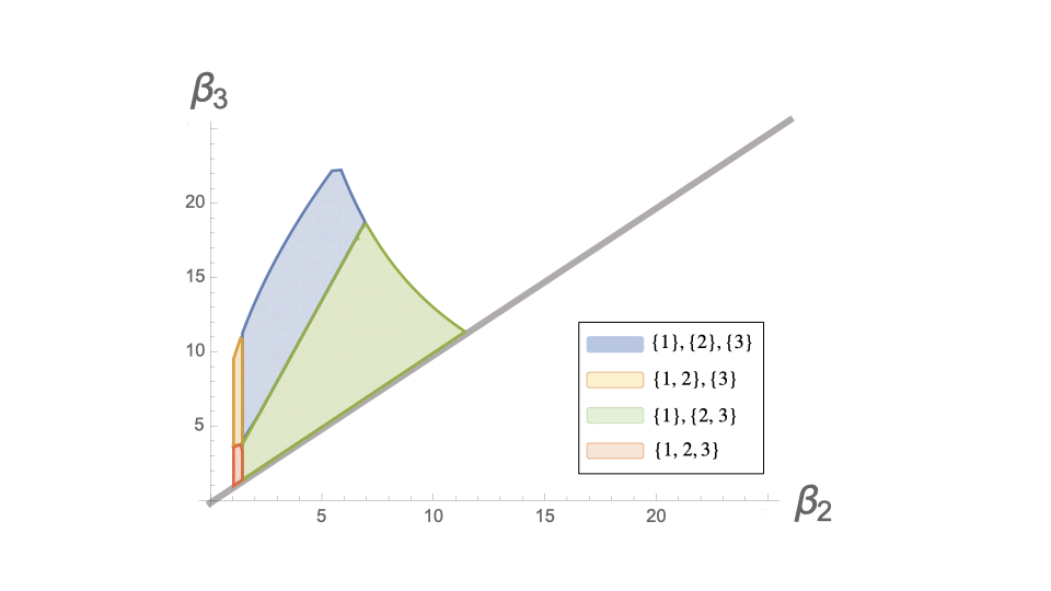
Figure 3: Equilibrium exit wave patterns when the optimal policy entails one exit wave including all three agents

When the cost multipliers are sufficiently close to one another, agents exit in unison even in equilibrium. When $\beta_{2}$ is sufficiently close to $1$, but $\beta_{3}$ is sufficiently higher, agent $3$ has substantially lower search costs. Since agents $1$ and $2$ do not internalize their externalities on agent $3$, they prefer to leave early on, generating two exit waves. Similarly, when $\beta_{2}$ and $\beta_{3}$ are sufficiently high but close to one another, two exit waves occur in equilibrium. Last, when agents’ costs are sufficiently different, equilibrium dictates agents exiting at different points, resulting in three exit waves, even when externalities are sufficiently strong so that the social planner would prefer to have the agents search together till they all exit. Naturally, for sufficiently high $\beta_{2}$ and $\beta_{3}$, the wedge in costs is big and even the social planner would prefer to split agents’ exits. The Online Appendix contains detailed characterization of the equilibrium and social planner’s solutions and displays similar figures for other exit-wave structures chosen by the social planner.

6 Conclusions and Discussion

This paper analyzes team search patterns. We show that the equilibrium and socially optimal search scopes are constant within an alliance. However, as alliance members depart, individual search scopes increase in equilibrium and decrease under the optimal policy. We also characterize the deterministic path of exit waves generated in equilibrium. In particular, even when team members are fully heterogeneous, clustered exits may occur. The optimal path of exit waves shares features with the equilibrium path in terms of the structure of stopping boundaries that govern departures. However, search externalities naturally prolong optimal search in teams and alter resulting exit waves.

In what follows, we consider two extensions of our model, explicit rewards for innovating early and the utilization of non-Markovian strategies in equilibrium. In the Online Appendix, we also analyze the limitations introduced by a fixed search scope that cannot be altered, and our model’s implications for settings with independent search observations.

6.1 Equilibrium with Penalties for Later Innovations

Suppose stopping earlier grants one an advantage. For example, a firm that produces the first product of its type might capture a market segment that is later more challenging to capture. Similarly, researchers arguably get additional credit for being the first to suggest a modeling framework or a measurement technique.

For simplicity, consider a team of two agents. Assume that the first agent to stop, say at time $t$, receives $M_{t}$. The second agent to stop, say at time $s>t$, receives $\alpha M_{s}$, with $\alpha\leq 1$. If both agents stop at the same time $t$, they both receive $M_{t}$. As we show in the Online Appendix, the order of exits remains deterministic. Furthermore, as long as both agents are searching, the search scope and the initial stopping boundary are identical to those in our benchmark setting, where $\alpha=1$. Thus, if there is a unique exit wave when $\alpha=1$, that is still the case when $\alpha<1$.

Suppose there are two distinct exit waves with $\alpha=1$. Then, there is a leader—the agent who exits early—and a follower—the agent who exits later. The leader’s stopping boundary $g_{L}(\cdot)$ remains her equilibrium stopping boundary regardless of $\alpha$ and is governed by the drawdown identified in Proposition 2. The follower’s stopping boundary, however, may change.

To characterize the follower’s stopping boundary, denote the costs of the leader by $c_{L}(\cdot)$ and those of the follower by $c_{F}(\cdot)$. Let $\sigma_{L}$ denote the leader’s search scope when searching within the full team, $\sigma_{T}$ denote the total search scope in the full team, and $\sigma_{F}$ denote the follower’s optimal solo search scope. Similar calculations to those underlying Proposition 2 yield the follower’s stopping boundary $g_{F}(\cdot)$:

$$g_{F}(M)=\begin{cases}M-\frac{\alpha\sigma_{F}^{2}}{2c_{F}(\sigma_{F})}\text{ if }M<\overline{M}\text{ and }\frac{\alpha\sigma_{F}^{2}}{2c_{F}(\sigma_{F})}>\frac{\sigma_{T}^{2}}{2c_{L}(\sigma_{L})},\\ g_{L}(M)\text{ otherwise,}\end{cases}$$

where

$$\overline{M}=\frac{1}{1-\alpha}\frac{c_{F}(\sigma_{F})}{\sigma_{F}^{2}}\left(\frac{\alpha\sigma_{F}^{2}}{2c_{F}(\sigma_{F})}-\frac{\sigma_{T}^{2}}{2c_{L}(\sigma_{L})}\right)^{2}\text{.}$$

To glean some intuition, consider the follower’s problem after the leader’s departure. The follower faces a similar problem to the individual agent’s problem, with identical search costs and rewards scaled down by $\alpha$. This case falls within the analysis of Urgun and Yariv (2021). The search scope is unaffected by the attenuated rewards, but the drawdown size is scaled linearly by $\alpha$—as $\alpha$ declines, the rewards from search become less meaningful, and the follower ceases search more willingly. Naturally, for sufficiently low $\alpha$, search continuation would not be worthwhile altogether, regardless of the maximal observation achieved when the leader exits. That corresponds to the drawdown used by the follower alone, $\frac{\alpha\sigma_{F}^{2}}{2c_{F}(\sigma_{F})}$, being smaller than the full alliance’s drawdown, $\frac{\sigma_{T}^{2}}{2c_{L}(\sigma_{L})}$. In that case, the stopping boundary of the leader governs the exit of both. In addition, when the maximal observation $M$ achieved when the leader exits is high enough, the loss from leaving at a later point, $(1-\alpha)M$ is substantial for any $\alpha<1$. For sufficiently high $M$, search continuation would again not be profitable. As $\alpha$ increases, the threshold level $\overline{M}$ increases. To summarize, for the follower to continue search after the leader, $\alpha$ needs to be sufficiently high and the current maximum sufficiently small.

Importantly, when later innovations are penalized, there are no preemption motives. The main impact is on later innovators, who face weakened incentives to search. Mechanically, larger exit waves occur for a larger set of parameters. Nonetheless, the main messages of the paper extend directly to such settings.

6.2 Non-Markovian Strategies

Our equilibrium analysis restricts attention to Markovian strategies. In our setting, the use of non-Markovian strategies cannot yield the socially optimal solution in general. To see why, consider a team of two agents and suppose the optimal search scope can be implemented in equilibrium—say, when there is only one viable scope, $\underline{\sigma}=\overline{\sigma}$. Our results show that the social planner would like agents to search for a longer time than the (Markovian) equilibrium we identify would prescribe. Suppose agent 1 is the first to exit in such an equilibrium, where stopping strategies are not weakly dominated given the search scopes. As long as agent 2 is searching, agent 1 has a unique best response. She would like to use a drawdown size $d_{1}$, while the social planner would like her to use a drawdown size $d\textquoteright_{1}>d_{1}$. However, regardless of the space of strategies, there is no way to punish agent $1$ for leaving early, and no way to foretell that she will do so. A full analysis of equilibria in non-Markovian strategies is left for the future.

Appendix A Appendix

Corollary proofs are immediate and, for completeness, available in the Online Appendix. In what follows, we provide proofs for the paper’s main results.

A.1 Proofs for Equilibrium Team Search

First, we note a useful lemma, commonly known as “reflection on the diagonal”. This lemma allows us to omit the partial derivatives pertaining to $M$ in the control problem in the various Hamilton-Jacobi-Bellman (HJB) equations that we will derive. Proofs of this result can be found in various sources, including Dubins et al. (1994), Urgun and Yariv (2021) and Peskir (1998) among others and hence omitted.

Lemma 1.

The infinitesimal generator of the two dimensional process $Z=(M,X)$ satisfies the following:

1. If $M_{t}>X_{t}$, then $\mathcal{A}_{Z}^{\sigma_{t}}=\mathcal{A}_{X}^{\sigma_{t}}=\frac{1}{2}(\sigma_{t})^{2}\frac{\partial^{2}}{\partial X^{2}}$.

2. If $M_{t}=X_{t}$, then $\frac{\partial V}{\partial M}=0$.

Proof of Proposition 1.

For any agent $i$ in an alliance $A$, the value function takes the following form

$$V_{i}^{A}(M,X)=\mathbb{E}\left[\int_{0}^{\tau^{A}}c_{i}(\sigma_{i,t}|M,X)dt+\mathbb{E}\left[V_{i}^{A}(M_{\tau^{A}},g^{A}(M_{\tau^{A}})\right]\right],$$ (2)

where

$$\mathbb{E}\left[V_{i}^{A}(M_{\tau^{A}},g^{A}(M_{\tau^{A}})\right]=\begin{cases}M_{\tau^{A}}\text{ if }g_{i}^{A}(M_{\tau^{A}})=g^{A}(M_{\tau^{A}})\\ V_{i}^{A\setminus\{j\}}\text{ if }g_{j}^{A}(M_{\tau^{A}})=g^{A}(M_{\tau^{A}})>g_{i}^{A}(M_{\tau^{A}}),j\in A\end{cases}.$$

In words, with Markov strategies, agent $i$’s expected value is derived from two components: the cost accrued until her alliance shrinks, and the continuation value once that happens. If the alliance shrinks with agent $i$’s departure, her continuation value is simply the maximum value when she exits.

For a given observed maximum $M$, there are two cases to consider for an active agent $i$ in $A$: either her stopping boundary is the highest within the active alliance, or not. We discuss these in sequence.

Suppose first that $g_{i}^{A}(M)=\max_{j\in A}g_{j}^{A}(M)$. Consider any observed value $X$ such that $g_{i}^{A}(M)\leq X\leq M$. The Green function on the interval $[a,b]$ is defined as follows:

$$\begin{aligned} G_{a,b}(x,y)&=\left\{\begin{array}[]{ll}\frac{(b-x)(y-a)}{b-a}&\text{ if }a<y<x<b\\ \frac{(b-y)(x-a)}{b-a}&\text{ if }a<x<y<b\end{array}\right.\end{aligned}.$$

Following standard techniques,we can write the equilibrium value function of agent $i$ in the following recursive fashion:

$$V_{i}^{A}(M,X) =M\frac{M-X}{M-g_{i}^{A}(M)}+V_{i}^{A}(M,M)\frac{X-g_{i}^{A}(M)}{M-g_{i}(M)}$$

$$-\int_{g_{i}^{A}(M)}^{M}G_{g_{i}^{A}(M),M}(x,y)c_{i}(\sigma_{i}^{A}(M,y))\frac{2}{(\sigma^{A}(M,y))^{2}}dy.$$

Rearranging terms, we get:

$$V_{i}^{A}(M,M)-M =\frac{M-g_{i}^{A}(M)}{X-g_{i}^{A}(M)}\left[V_{i}^{A}(M,X)-M\right.$$

$$\left.+\int_{g_{i}^{A}(M)}^{M}G_{g_{i}^{A}(M),M}(x,y)c_{i}(\sigma_{i}^{A}(M,y))\frac{2}{(\sigma^{A}(M,y))^{2}}dy\right].$$

Since agent $i$ optimally terminates her search at $g_{i}^{A}(M)$, smooth pasting must hold at $g_{i}^{A}(M)$. The derivative of the continuation value as $X\rightarrow g_{i}^{A}(M)$ can be written as $\lim_{X\rightarrow g_{i}^{A}(M)}\frac{V_{i}^{A}(M,X)-M}{X-g_{i}^{A}(M)}$. By smooth pasting, this must be equal the derivative of the value from stopping, $\frac{\partial}{\partial x}M=0$.

Consider then the above equality for $V_{i}^{A}(M,M)$. Taking the limit as $X\rightarrow g_{i}^{A}(M)$,

$$V_{i}^{A}(M,M)=M+\int_{g_{i}(M)}^{M}(M-y)c_{i}(\sigma_{i}^{A}(y))\frac{2}{(\sigma^{A}(y))^{2}}dy.$$

This, in turn, implies that

$$V_{i}^{A}(M,X)=M+\int_{g_{i}^{A}(M)}^{X}(X-y)c_{i}(\sigma_{i}^{A}(y))\frac{2}{(\sigma^{A}(y))^{2}}dy.$$

Now, taking the second derivative with respect to $X$ and simplifying yields:

$$\frac{\partial^{2}V_{i}^{A}(M,X)}{\partial X^{2}}=\frac{2c_{i}(\sigma_{i}^{A}(M,X))}{(\sigma_{i}^{A}(M,X))^{2}}.$$

Plugging this back into the HJB for agent $i$ and simplifying further yields:

$$\frac{2c_{i}(\sigma_{i}^{A}(M,X))}{c^{\prime}_{i}(\sigma_{i}^{A}(M,X))}=\sigma_{i}^{A}(M,X)+\sum_{j\in A\setminus\{i\}}\sigma_{j}^{A}(M,X).$$

Suppose now that $i$ does not have the highest stopping boundary: $\max_{k\in A}g_{k}^{A}(M)>g_{i}^{A}(M)$. Let $F(M)=\{j\in N:\max_{k\in A}g_{k}^{A}(M)=g_{j}^{A}(M)\}$. Choose an arbitrary agent $j\in F(M)$. As above, we can write the continuation payoff of $i$ as follows:

$$V_{i}^{A}(M,X) =V_{i}^{A}(M,g_{i}^{A}(M))\frac{M-X}{M-g_{j}^{A}(M)}+V_{i}^{A}(M,M)\frac{X-g_{j}^{A}(M)}{M-g_{j}(M)}$$

$$-\int_{g_{j}^{A}(M)}^{M}G_{g_{j}^{A}(M),M}(X,y)c_{i}(\sigma_{i}^{A}(M,y))\frac{2}{(\sigma^{A}(M,y))^{2}}dy.$$

Rearranging terms, we get:

$$V_{i}^{A}(M,M)-V_{i}^{A}(M,g_{j}^{A}(M)) =\frac{M-g_{j}^{A}(M)}{X-g_{j}^{A}(M)}\left[V_{i}^{A}(M,X)-V_{i}^{A}(M,g_{j}^{A}(M))\right.$$

$$+\left.\int_{g_{j}^{A}(M)}^{M}G_{g_{j}^{A}(M),M}(X,y)c_{i}(\sigma_{i}^{A}(M,y))\frac{2}{(\sigma^{A}(M,y))^{2}}dy\right].$$

Again, taking the limit as $X\rightarrow g(M)$ from above, and letting $\frac{\partial_{D}V_{i}^{A}(M,g(M))}{\partial X}$ denote the upper Dini derivative of $V_{i}^{A}(M,g(M))$ at $g(M)$, we have:

$$V_{i}^{A}(M,M) =\frac{\partial_{D}V_{i}^{A}(M,g(M))}{\partial X}(M-g(M))+V_{i}^{A}(M,g_{j}^{A}(M))$$

$$+\int_{g_{j}(M)}^{M}(M-y)c_{i}(\sigma_{i}^{A}(M,y))\frac{2}{(\sigma^{A}(M,y))^{2}}dy.$$

Plugging this identity in $V_{i}^{A}(M,X)$’s expression and taking the second derivative:

$$\frac{\partial^{2}V_{i}^{A}(M,X)}{\partial X^{2}}=\frac{2c_{i}(\sigma_{i}^{A}(M,X))}{(\sigma_{i}^{A}(M,X))^{2}}.$$

Plugging this back into the HJB for agent $i$ and simplifying further generates:

$$\frac{2c_{i}(\sigma_{i}^{A}(M,X))}{c^{\prime}_{i}(\sigma_{i}^{A}(M,X))}=\sigma_{i}^{A}(M,X)+\sum_{k\in A\setminus\{i\}}\sigma_{k}^{A}(M,X).$$

Our assumption that the cost function’s second derivative is bounded above zero implies that the conditions of Theorem 6.4 of Fleming and Rishel (2012) are satisfied. Hence, any equilibrium features continuous search scopes within any alliance. In particular, within an active alliance, agents can utilize only one of the solutions for the system above. ∎

Proof of Proposition 2.

The statement of Proposition 2 is a combination of the following claims.

Claim 1.

For any given alliance $A$ with $i\in A$, if $g_{i}^{A}(M^{\ast})=\max_{j\in A}g_{j}^{A}(M^{\ast})$ for some $M^{\ast}$, then $g_{i}^{A}(M)=\max_{j\in A}g_{j}^{A}(M)$ for all $M$.

Proof of Claim.

The proof of the claim relies on the following lemma.

Lemma 2.

Suppose agent $i\in A$ has the highest stopping boundary at a given observed $M,X$. Then $g_{i}^{A}(M)$ is a drawdown stopping boundary.

Proof of Lemma 2.

Suppose $\max_{j\in A}g_{j}^{A}(M)=g_{i}^{A}(M)$. As shown in the proof of Proposition 1, we have

$$V_{i}^{A}(M,X)=M+\int_{g_{i}^{A}(M)}^{X}(X-y)c_{i}(\sigma_{i}^{A}(M,y))\frac{2}{(\sigma^{A}(M,y))^{2}}dy.$$

Furthermore using Proposition 1 we know that $\sigma^{A}(M,X)=\sigma^{A}$ for all $M,X$ and $\sigma_{i}^{A}(M,X)=\sigma_{i}^{A}$ for all $M,X$.

Now, differentiating $V_{i}^{A}(M,X)$ with respect to $M$ and evaluating the derivative at $X=M$ yields the following ordinary differential equation (ODE) for $g_{i}^{A}(M)$:

$$g_{i}^{A}(M)^{\prime}=\frac{(\sigma^{A})^{2}}{2c_{i}(\sigma_{i}^{A})\left(M-g_{i}^{A}(M)\right)},$$

which leads to the following solution:

$$g_{i}^{A}(M)=M-\frac{(\sigma^{A})^{2}}{2c_{i}(\sigma_{i}^{A})}.$$

This is a drawdown stopping boundary with drawdown size $d^{A}_{i}:=\frac{(\sigma^{A})^{2}}{2c_{i}(\sigma_{i}^{A})}$. ∎

We can now proceed with the claim’s proof. Towards a contradiction, suppose that $\max_{j\in A}g_{j}^{A}(M)=g_{i}^{A}(M)$ for some $M$. Suppose $M^{\prime}=\inf_{\hat{M}>M}\{M|i\notin\arg\max_{j\in A}g_{j}^{A}(\hat{M})\}$ and that for some $\varepsilon>0$, for any $\hat{M}\in(M^{\prime},M^{\prime}+\varepsilon),$ for some $k\neq i$, we have $\max_{j\in A}g_{j}^{A}(M^{\prime})=g_{k}^{A}(M^{\prime})>g_{i}^{A}(M^{\prime})$. From continuity of the stopping boundary and Lemma 2,

$$g_{i}^{A}(M)=M-\frac{(\sigma^{A})^{2}}{2c_{i}(\sigma_{i}^{A})}\text{ \ \ \ and \ \ \ }g_{k}^{A}(M^{\prime})=M^{\prime}-\frac{(\sigma^{A})^{2}}{2c_{k}(\sigma_{k}^{A})}.$$

Our choice of $i$ and $k$ yields $\frac{(\sigma^{A})^{2}}{2c_{i}(\sigma_{i}^{A})}\leq\frac{(\sigma^{A})^{2}}{2c_{k}(\sigma_{k}^{A})}$ and $\frac{(\sigma^{A})^{2}}{2c_{i}(\sigma_{i}^{A})}>\frac{(\sigma^{A})^{2}}{2c_{k}(\sigma_{k}^{A})}$, in contradiction. ∎

Claim 2.

Suppose that for some $i$ in an active alliance of $A$, $\frac{(\sigma^{A})^{2}}{2c_{i}(\sigma_{i}^{A})}\leq\frac{(\sigma^{A})^{2}}{2c_{j}(\sigma_{j}^{A})}$ for all $j\in A$. Then $i$ is the first to exit alliance $A$.

Proof of Claim.

Suppose $\frac{(\sigma^{A})^{2}}{2c_{i}(\sigma_{i}^{A})}\leq\frac{(\sigma^{A})^{2}}{2c_{j}(\sigma_{j}^{A})}$ for all $j\in A$ but that agent $i$ is not one of the first agents to exit from alliance $A$ for some path of observed values. For that path, agent $i$ ceases her search when active at a smaller alliance $A\setminus K$. Without loss of generality, suppose agent $j$ exits alliance $A$ first (if there are multiple such agents, pick any) when observing $M$ and $X$. From Lemma 2, agent $j$’s stopping boundary is characterized by a drawdown. However, from the Claim’s restriction,

$$M-\frac{(\sigma^{A})^{2}}{2c_{j}(\sigma_{j}^{A})}\leq M-\frac{(\sigma^{A})^{2}}{2c_{i}(\sigma_{i}^{A})}.$$

For each $k\in A$, the stopping boundary $g_{k}^{A}(M)=M-\frac{(\sigma^{A})^{2}}{2c_{k}(\sigma_{k}^{A})}$ is identified by value matching and smooth pasting. In particular, we have $V_{k}^{A}(M,g_{k}^{A}(M))=M$. If $g_{i}^{A}(M)>g_{j}^{A}(M)$, this implies that $V_{i}^{A}(M,g_{j}^{A}(M)+\epsilon)<M$ for $0<\epsilon<\frac{(\sigma^{A})^{2}}{2c_{j}(\sigma_{j}^{A})}-\frac{(\sigma^{A})^{2}}{2c_{i}(\sigma_{i}^{A})}$. Therefore, agent $i$ would prefer to stop strictly before agent $j$. ∎

The two claims and Lemma 2’s characterization yield the proposition’s proof.

∎

A.2 Proofs for the Social Planner’s Solution

Proof of Proposition 3.

Let $\left\{\sigma_{i}^{A}(M,X,A)\right\}$ and $G(M,X,A)$ correspond to a solution to the social planner’s problem. Consider any alliance $A_{k}$ at some observed values and let $A_{k+1}$ denote the potentially empty random alliance dictated by this optimal solution. Optimality implies that the induced search scopes with $A_{k}$ should solve:

$$\sup_{\{\sigma_{i,t}\}_{i\in A_{k}}}\mathbb{E}\left[|A_{k}\setminus A_{k+1}|M_{\tau^{A_{k}}}-\int_{0}^{\tau^{A_{k}}}\sum_{i\in A_{k}}c_{i}(\sigma_{i,t}^{A_{k}})dt\right].$$

Following similar steps to the proof of proposition 1 in the equilibrium analysis, the continuation HJB for the social planner can be written as:

$$\frac{\partial^{2}W(M,X,A_{k})}{\partial X^{2}}=\frac{\partial^{2}\mathbb{E}\left[\int_{0}^{\tau^{A_{k}}}\sum_{i\in A_{k}}c_{i}(\sigma_{i}^{A_{k}}(X))dt|M,X\right]}{\partial X^{2}}.$$

It follows that

$$\frac{2\sum_{i\in A_{k}}c_{i}(\sigma_{i}^{A_{k}}(X))}{\sum_{i\in A_{k}}\sigma_{i}^{A_{k}}(X)}=c_{j}^{\prime}(\sigma_{i}^{A_{k}}(X))\quad\forall j\in A_{k}.$$

Since there is no direct dependence on $X$ on either side, optimal search scopes are independent of observed values and constant over time for each active alliance.

∎

Proof of Proposition 4.

The proof follows from two lemmas:

Lemma 3.

If the set of agents exitting an alliance is independent of the observed path, each alliance has a stopping boundary identified by a drawdown size $d_{A_{k}}$.

Proof of Lemma 3.

Let $A_{K}$ be the final alliance in the social planner’s problem, with cardinality $|A_{K}|$. The social planner’s problem when left with alliance $A_{K}$, and observing maximum $M$ and current value $X$, takes the following form:

$$W_{K}(M,X)=\sup_{\tau^{K},\{\sigma_{i}\}_{\imath\in A_{K}}}\mathbb{E}\left[|A_{K}|M_{\tau^{K}}-\int_{0}^{\tau^{K}}\sum_{i\in A_{K}}c_{i}(\sigma_{i}^{A_{K}})dt\text{ \ }|\text{ \ }M,X\right].$$

This is tantamount to a single-searcher problem, where search rewards are scaled by $|A_{K}|$. From Urgun and Yariv (2021), the stopping boundary is given by:

$$g^{A_{K}}(M)=M-d_{A_{k}},$$

where $d_{A_{k}}=\frac{|A_{K}|\sigma^{A_{K}}}{2\sum_{i\in A_{K}}c_{i}(\sigma_{i}^{A_{K}})}$.

Consider the social planner’s problem when the penultimate alliance $A_{K-1}$ is active and the observed maximum and value are $M$ and $X$, respectively:

$$W_{K-1}(M,X) =\sup_{\tau^{K-1},\{\sigma_{i}\}_{\imath\in A_{K-1}}}\mathbb{E}\left[|A_{K-1}\setminus A_{K}|M_{\tau^{K-1}}+W_{K}(M_{\tau^{K-1}},g^{A_{K-1}}(M_{\tau^{K-1}}))\text{ \ }|\text{ \ }M,X\right]$$

$$-\mathbb{E}\left[\int_{0}^{\tau^{K-1}}\sum_{i\in A_{K-1}}c_{i}(\sigma_{i}^{A_{K-1}})dt\text{ \ }|\text{ \ }M,X\right].$$

By optimality of the stopping time $\tau^{K-1}$, we have smooth pasting of $W_{K-1}(M,X)$ and $W_{K}(M,X)$. Therefore,

$$W_{K-1}(M,g^{A_{K-1}}(M)) =|A_{K-1}\setminus A_{K}|M+W_{K}(M,g^{A_{K-1}}(M)),$$

$$\frac{\partial W_{K-1}(M,g^{A_{K-1}}(M))}{\partial X}{\large|_{X=g^{A_{k-1}}}} {\large=\frac{\partial(|A_{K-1}\setminus A_{K}|M+W_{K}(M,g^{A_{K-1}}(M)))}{\partial X}|_{X=g^{A_{K-1}}(M)}}.$$

Similar to our equilibrium analysis, and using the notation for the Green function introduced there, we can write the welfare maximization problem as

$$W_{K-1}(M,X)=|A_{K-1}\setminus A_{K}|M+W_{K}(M,g^{A_{K-1}}(M))\frac{M-X}{M-g^{A_{K-1}}(M)}$$

$$+W_{K-1}(M,M)\frac{X-g_{A^{K-1}}(M)}{M-g^{A_{K-1}}(M)}-\int_{g^{A_{K-1}}}^{M}G_{g^{A_{K-1}}(M),M}(X,y)\frac{2\sum_{i\in A_{K-1}}c_{i}(\sigma_{i}^{A_{K-1}})}{(\sigma^{A_{K-1}})^{2}}dy.$$

Letting $X$ approach $g^{A_{K-1}}(M)$, smooth pasting and rearranging yields:
$W_{K-1}(M,X)=|A_{K-1}\setminus A_{K}|M+W_{K}(M,g^{A_{K-1}}(M))$
$+\left(X-g^{A_{K-1}}(M)\right)\int_{g^{A_{K}}(M)}^{g^{A_{K-1}}(M)}\frac{2\sum_{i\in A_{K}}c_{i}(\sigma_{i}^{A_{K}})}{(\sigma^{A_{K}})^{2}}dx+\int_{g^{A_{K-1}}(M)}^{X}(X-y)\frac{2\sum_{i\in A_{K-1}}c_{i}(\sigma_{i}^{A_{K-1}})}{(\sigma^{A_{K-1}})^{2}}dy,$

Using the closed-form representation of $W_{K}$ leads to:

$$W_{K-1}(M,X)=|A_{K-1}|M+\frac{1}{2}(g^{A_{K-1}}(M)-g^{A_{K}}(M))^{2}\frac{2\sum_{i\in A_{K}}c_{i}(\sigma_{i}^{A_{K}})}{(\sigma^{A_{K}})^{2}}$$

$$+\left(X-g^{A_{K-1}}(M)\right)(g^{A_{K-1}}(M)-g^{A_{K}}(M))\frac{2\sum_{i\in A_{K}}c_{i}(\sigma_{i}^{A_{K}})}{(\sigma^{A_{K}})^{2}}$$

$$+\frac{1}{2}(X-g^{A_{K-1}}(M))^{2}\frac{2\sum_{i\in A_{K-1}}c_{i}(\sigma_{i}^{A_{K-1}})}{(\sigma^{A_{K-1}})^{2}}.$$

To generate an ODE that identifies $g^{A_{K-1}}(M)$, we take the derivative with respect to $M$ that, evaluated at $X=M$, should equal $0$. After some algebraic manipulations, this ODE take the form

$$\frac{dg^{A_{K-1}}(M)}{dM}=\frac{|A_{K-1}\setminus A_{K}|}{2\left(M-g^{A_{K-1}}(M)\right)\left(\frac{\sum_{i\in A_{K-1}}c_{i}(\sigma_{i}^{A_{K-1}})}{(\sigma^{A_{K-1}})^{2}}-\frac{\sum_{i\in A_{K}}c_{i}(\sigma_{i}^{A_{K}})}{(\sigma^{A_{K}})^{2}}\right)}.$$

It is straightforward to verify that the unique solution for this ODE satisfying the value-matching condition takes the form $g^{A_{K-1}}(M)=M-d_{A_{K-1}}$, where

$$d_{A_{K-1}}=\frac{|A_{K-1}\setminus A_{K}|}{2\left(\frac{\sum_{i\in A_{K-1}}c_{i}(\sigma_{i}^{A_{K-1}})}{(\sigma^{A_{K-1}})^{2}}-\frac{\sum_{i\in A_{K}}c_{i}(\sigma_{i}^{A_{K}})}{(\sigma^{A_{K}})^{2}}\right)}.$$

In particular, the optimal stopping boundary is a drawdown stopping boundary.

Proceeding inductively, for any alliance $m\leq K$, the continuation value when $M$ and $X$ are observed can be written as:

$$W_{m}(M,X)= |A_{m}\setminus A_{m+1}|M+W_{m+1}(M,g^{A_{m}}(M))$$

$$+\left(X-g^{A_{m}}(M)\right)\sum_{k=m}^{K-1}\left(\int_{g^{k+1}(M)}^{g^{k}(M)}\frac{2\sum_{i\in A_{k+1}}c_{i}(\sigma_{i}^{A_{k+1}})}{(\sigma^{A_{k+1}})^{2}}dx\right)$$

$$- \int_{g^{A_{m}}(M)}^{X}(X-y)\frac{2\sum_{i\in A_{m}}c_{i}(\sigma_{i}^{A_{m}})}{(\sigma^{A_{m}})^{2}}dy.$$

We can then repeat the steps above to generate an analogous ODE for $g^{A_{m}}(M)$ and verify that it is uniquely identified as a drawdown stopping boundary. Namely, $g^{A_{m}}(M)=M-d_{A_{m}}$, where

$$d_{A_{m}}=\frac{|A_{m}\setminus A_{m+1}|}{2\left(\frac{\sum_{i\in A_{m}}c_{i}(\sigma_{i}^{A_{m}})}{(\sigma^{A_{m}})^{2}}-\frac{\sum_{i\in A_{m+1}}c_{i}(\sigma_{i}^{A_{m+1}})}{(\sigma^{A_{m+1}})^{2}}\right)}.$$

∎

Lemma 4.

The set of agents dropping from an alliance is deterministic. That is for any alliance $A$, for all pairs $(M,X),(M^{\prime},X^{\prime})$ such that $G(M,X,A)\neq A$, we have $G(M,X,A)=G(M^{\prime},X^{\prime},A)$.

Proof of Lemma 4.

We prove this result by induction on the size of the initial team $N$, regardless of the starting values of the maximum and the current value. The claim follows immediately for $N=1$. In that case, the agent uses a drawdown stopping boundary and the only way for the singleton alliance to change is for the agent to terminate her search.

For the inductive step, assume that for any initial team of size $N-1$ or less the optimal alliance sequence is deterministic. By Lemma 3, each of these alliances is associated with a drawdown stopping boundary. Let $A_{1}$ be an alliance of size $N$. The continuation value when $M$ and $X$ are observed is:

$$W_{1}(M,X)=\mathbb{E}\left[M_{\tau^{1}}+\max_{A_{2}\subsetneq A_{1}}\{|A_{1}\setminus A_{2}|M_{\tau^{1}}+W_{A_{2}}(M_{\tau^{1}},g^{A_{1}}(M_{\tau^{1}}))\}-\int_{0}^{\tau^{1}}\sum_{i\in A_{k}}c_{i}(\sigma_{i}^{A_{1}})dt\right].$$

Suppose that, for some path, the social planner optimally transitions from alliance $A_{1}$ to a strictly smaller alliance $A_{2}\neq\emptyset$. In particular, alliance $A_{2}$ contains fewer than $N$ agents. By the inductive hypothesis, the sequence that ensues is path independent. We can therefore write the continuation value as:

$$W_{1}(M,X)= |A_{1}\setminus A_{2}|M+W_{2}(M,g^{A_{1}}(M))$$

$$+\left(X-g^{A_{1}}(M)\right)\sum_{m=2}^{K-1}\left(\int_{g^{A_{m+1}}(M)}^{g^{A_{m}}(M)}\frac{2\sum_{i\in A_{m+1}}c_{i}(\sigma_{i}^{A_{m+1}})}{(\sigma^{A_{m+1}})^{2}}dx\right)$$

$$+ \int_{g^{A_{1}}(M)}^{X}(X-y)\frac{2\sum_{i\in A_{1}}c_{i}(\sigma_{i}^{A_{1}})}{(\sigma^{A_{1}})^{2}}dy.$$

As before, this yields an ODE characterizing $g^{A_{1}}(M)$ and a unique solution of the form $g^{A_{1}}(M)=M-d_{A_{1}}$, where $d_{A_{1}}=\frac{|A_{1}\setminus A_{2}|}{2\left(\frac{\sum_{i\in A_{1}}c_{i}(\sigma_{i}^{A_{1}})}{(\sigma^{A_{1}})^{2}}-\frac{\sum_{i\in A_{2}}c_{i}(\sigma_{i}^{A_{2}})}{(\sigma^{A_{2}})^{2}}\right)}$. Towards a contradiction, suppose that at some other path a different alliance is optimally chosen to follow the full alliance $A_{1}$. Call that alliance $\hat{A}_{2}\neq A_{2}$. Similar argument would then imply that the stopping boundary for $A_{1}$ is given by $g^{A_{1}}(M)=M-\hat{d}_{A_{1}}$, where $\hat{d}_{A_{1}}=\frac{|A_{1}\setminus\hat{A}_{2}|}{2\left(\frac{\sum_{i\in A_{1}}c_{i}(\sigma_{i}^{A_{1}})}{(\sigma^{A_{1}})^{2}}-\frac{\sum_{i\in\hat{A}_{2}}c_{i}(\sigma_{i}^{\hat{A}_{2}})}{(\sigma^{\hat{A}_{2}})^{2}}\right)}$. Suppose $d_{A_{1}}=d_{\hat{A}_{1}}$. Without loss of generality, assume $\sigma^{A_{2}}\geq\sigma^{\hat{A}_{2}}$. We cannot have $\hat{A}_{2}\subseteq A_{2}$. Indeed, if that were the case, the social planner would be indifferent between keeping the agents in $A_{2}\setminus\hat{A}_{2}$ at points at which either $\hat{A}_{2}\$or $A_{2}$ are chosen to continue. However, our tie-breaking rule implies that such indifferences are broken in favor of stopping; that is, in such cases, the smaller set $\hat{A}_{2}$ would be chosen. Therefore, $\hat{A}_{2}\nsubseteqq A_{2}$ and there exists an agent $i\in\hat{A}_{2}\setminus A_{2}$. Suppose that whenever the social planner transitions from $A_{1}$ to $A_{2}$, she instead transitions to $A_{2}\cup\{i\}$, maintaining the search scopes of members of $A_{2}$ as before and having agent $i$ search with the lowest scope $\sigma$ for a sufficiently small interval of time. In that interval of time, everyone in $A_{2}$ benefits. When alliance $\hat{A}_{2}$ is picked, agent $i$ uses at least as high a search scope, while benefitting from lower overall search scope. In particular, agent $i$ benefits as well from this change.

Suppose $d_{A_{1}}\neq d_{\hat{A}_{1}}$. In this case, the two stopping boundaries identified above, $M-d_{A_{1}}$ and $M-d_{\hat{A}_{1}}$ never intersect, in contradiction. ∎

Combining the two lemmas leads to the conclusion of the proposition. ∎

A.3 Proofs for Optimal Sequencing with Well-ordered Costs

Proof of Lemma 1.

As introduced in the proof of Corollary 3, we use here the superscripts $eq$ and $sp$ to denote the equilibrium and social planner’s solution, respectively. When costs are well-ordered, in equilibrium, in any alliance, all agents utilize the same search scope. In particular, for any active alliance $A$ and any $i,j\in A$, we have $\sigma_{i}^{A,eq}=\sigma_{j}^{A,eq}$. This implies that, in equilibrium, each agent $k$ exits no later than agent $k-1$, for all $k=2,...,N$. Indeed, in any active alliance $A$, the equilibrium stopping boundary is governed by drawdown size

$$d_{A}^{eq}=\min_{i\in A}\frac{(\sigma^{A,eq})^{2}}{2c_{i}(\sigma_{i}^{A,eq})}=\max_{i\in A}\frac{(\sigma^{A,eq})^{2}}{2c_{i}(\sigma_{i}^{A,eq})}.$$

Suppose, towards a contradiction, that there exists a pair $i,j$ such that $i>j$, so that $\beta_{i}>\beta_{j}$, and the social planner has agent $i$ terminate her search strictly before agent $j$. There are then two distinct alliances in the social planner’s solution, $A_{k}$ and $A_{m},$ with $k<m$, where $i,j\in A_{k}$ but $i\notin A_{k+1}$ and $j\in A_{m}$ but $j\notin A_{m+1}$.

As we showed, the social planner’s solution associates a drawdown stopping boundary with each alliance. Denote the corresponding drawdown sizes $d_{k}^{sp}$ and $d_{m}^{sp}$ for $A_{k}$ and $A_{m}$, respectively. Suppose that, instead, the social planner swaps the exits of agents $i$ and $j$, exiting agent $j$ from $A_{k}$ whenever agent $i$ was to cease her search and exit from $A_{k}$ and exiting agent $i$ from $A_{m}$ whenever agent $j$ was to cease her search and exit from $A_{m}$. Furthermore, the social planner can have agent $i$ use the same search scope as agent $j$ had originally in the alliances that follow $A_{k}$. The overall search scope in any alliance does not change after this modification. Consequently, expected search outcomes are unaltered. However, the overall cost decreases weakly in every alliance and strictly in all alliances $A_{k+1},...,A_{m}$, contradicting the optimality of the proposed solution. ∎

Proof of Proposition 5.

Recall that our results so far imply that the social planner can restrict attention to the choice between deterministic alliance sequences. Furthermore, given a deterministic sequence of alliances, Lemma 3 identifies the optimal drawdown stopping boundaries associated with that alliance sequence. If the chosen sequence is suboptimal, some of its associated drawdown sizes might be negative or zero, implying the corresponding alliance is utilized for no length of time. This observation helps us to identify the optimal sequence. The proof of Proposition 5 follows from several lemmas. For any alliance $B_{k}$, regardless of whether it is on the social planner’s optimal alliance sequence, we denote the optimal overall search scope within the alliance by $\tilde{\sigma}^{k}$ and the consequent overall search cost within that alliance by $\tilde{c}^{k}$.

Lemma 5.

For any $m,j,k$ such that $m<j<k$, if the welfare-maximizing sequence is such that $B_{k}$ is preceded by $B_{m}$, then for any sequence where $B_{k}$ is preceded by $B_{j}$, we have $d_{B_{m}\rightarrow B_{k}}>d_{B_{j}\rightarrow B_{k}}$.

Proof of Lemma 5.

from the characterization of drawdowns in the well-ordered settings, $d_{B_{m}\rightarrow B_{k}}\neq d_{B_{j}\rightarrow B_{k}}$. Suppose that $d_{B_{m}\rightarrow B_{k}}<d_{B_{j}\rightarrow B_{k}}$. Since $B_{k}$ is preceded by $B_{m}$ in the optimal sequence, $d_{B_{m}\rightarrow B_{k}}>0$. It then follows that $d_{B_{j}\rightarrow B_{k}}>0$. This implies that it would be beneficial for the planner to have alliance $B_{m}$ first transition to alliance $B_{j}$, and only then transition to alliance $B_{k}$. ∎

Lemma 6.

If $m<k$, $d_{B_{m}\rightarrow\emptyset}>d_{B_{k}\rightarrow\emptyset}$ implies $d_{B_{m}\rightarrow B_{k}}>d_{B_{k}\rightarrow\emptyset}$.

Proof of Lemma 6.

$d_{B_{m}\rightarrow\emptyset}>d_{B_{k}\rightarrow\emptyset}$ implies

$$\frac{1}{N-m}\frac{\tilde{c}^{m}}{\tilde{\sigma}^{m}} <\frac{1}{N-k}\frac{\tilde{c}^{k}}{\tilde{\sigma}^{k}}\Longrightarrow\frac{1}{k-m}(\frac{\tilde{c}^{m}}{\tilde{\sigma}^{m}}-\frac{\tilde{c}^{k}}{\tilde{\sigma}^{k}})<\frac{1}{N-k}\frac{\tilde{c}^{k}}{\tilde{\sigma}^{k}},$$

illustrating the claim. ∎

Lemma 7.

For any $k$ such that $d_{B_{k}\rightarrow\emptyset}>d_{B_{N}\rightarrow\emptyset}>d_{B_{k+1}\rightarrow\emptyset}$, we have $d_{B_{k}\rightarrow B_{k+1}}>d_{B_{N}\rightarrow\emptyset}$.

Proof of Lemma 7.

Observe that $d_{B_{k}\rightarrow\emptyset}>d_{B_{N}\rightarrow\emptyset}>d_{B_{k+1}\rightarrow\emptyset}$ implies

$$(N-k+1)\frac{\tilde{c}^{N}}{\tilde{\sigma}^{N}}>\frac{\tilde{c}^{k+1}}{\tilde{\sigma^{k+1}}}\text{ \ \ \ and \ \ \ }\frac{\tilde{c}^{k}}{\tilde{\sigma}^{k}}>(N-k)\frac{\tilde{c}^{N}}{\tilde{\sigma}^{N}}.$$

Simply summing the inequalities and reorganizing yields the implied statement. ∎

Lemma 8.

If $d_{B_{k}\rightarrow\emptyset}>d_{B_{k-1}\rightarrow B_{k}}$, then $d_{B_{k}\rightarrow\emptyset}>d_{B_{k-1}\rightarrow\emptyset}>d_{B_{k-1}\rightarrow B_{k}}.$

Proof of Lemma 8.

From the first inequality, $d_{B_{k}\rightarrow\emptyset}>d_{B_{k-1}\rightarrow B_{k}}$, we have,

$$\frac{1}{N-k}\frac{\tilde{c}^{k}}{\tilde{\sigma}^{k}} <\frac{\tilde{c}^{k-1}}{\tilde{\sigma}^{k-1}}-\frac{\tilde{c}^{k}}{\tilde{\sigma}^{k}}\Longrightarrow\frac{N-(k-1)}{N-k}\frac{\tilde{c}^{k}}{\tilde{\sigma}^{k}}<\frac{\tilde{c}^{k-1}}{\tilde{\sigma}^{k-1}}\Longrightarrow d_{B_{k}\rightarrow\emptyset}>d_{B_{k-1}\rightarrow\emptyset}.$$

But this inequality implies that

$\frac{1}{N-k}\frac{\tilde{c}^{k}}{\tilde{\sigma}^{k}}<\frac{1}{N-(k-1)}\frac{\tilde{c}^{k-1}}{\tilde{\sigma}^{k-1}}\Longrightarrow\frac{\tilde{c}^{k-1}}{\tilde{\sigma}^{k-1}}-\frac{\tilde{c}^{k}}{\tilde{\sigma}^{k}}>\frac{1}{(N-(k-1))}\frac{\tilde{c}^{k-1}}{\tilde{\sigma}^{k-1}}\Longrightarrow d_{B_{k-1}\rightarrow\emptyset}>d_{B_{k-1}\rightarrow B_{k}}.$

∎

Lemma 9.

If $k$ satisfies $\max_{j}d_{B_{j}\rightarrow\emptyset}=d_{B_{k}\rightarrow\emptyset}$, then any alliance $B_{l}$ with $l<k$ cannot be the welfare maximizing last alliance.

Proof of Lemma 9.

Suppose not, so that, form some $l<k$, alliance $B_{l}$ is the last. Since $B_{k}$ is strictly contained in $B_{l}$, from the characterization of drawdowns in the well-ordered settings, $d_{B_{k}\rightarrow\emptyset}\neq d_{B_{l}\rightarrow\emptyset}.$ The social planner would, then, benefit from transitioning from $B_{l}$ to $B_{k}$ instead of exiting all members of $B_{l}$ since $d_{B_{k}\rightarrow\emptyset}>d_{B_{l}\rightarrow\emptyset}>0$, in contradiction. ∎

Lemma 10.

If $k$ satisfies $\max_{j}d_{B_{j}\rightarrow\emptyset}=d_{B_{k}\rightarrow\emptyset}$, then any alliance $B_{l}$ with $l>k$ cannot be the last.

Proof of Lemma 10.

We use induction on the cardinality of the set $B_{k}$. The claim certainly holds when $\left|B_{k}\right|=1$, so that $B_{k}=B_{N}=\{N\}$.

For the proof, it is useful to notice that our entire analysis does not hinge on the range of viable search scopes coinciding across agents. In fact, the analysis would go through in its entirety if each agent $i$ had an individual range of scope $[\underline{\sigma}_{i},\overline{\sigma}_{i}]$, as long as all solutions remain interior.

Assume the statement is true for sets up to cardinality $n$. We show the statement holds for $\left|B_{k}\right|=n+1$ (so that $k=N-n+1$). By Lemma 9, the last alliance cannot be $B_{j}$ with $j<k$. Towards a contradiction, suppose that a smaller set $B_{m}$, with $m>k$, is the last alliance. From the inductive hypothesis, we must have $d_{B_{m}\rightarrow\emptyset}>d_{B_{l}\rightarrow\emptyset}$ for all $l>m$, as otherwise the social planner would benefit by inducing $B_{l}$ to continue search instead of terminating it for all agents in $B_{m}$.

Suppose that $m<N$. Consider an equivalent problem, where alliance $B_{m}\$is replaced with a single individual $M$ that has cost function $\hat{c}(\cdot)$ defined so that $\hat{c}(\sigma)$ is the minimal overall cost in $B_{m}$ required for implementing an overall search scope $\sigma$. That is, if

$$\sigma_{m}^{B_{m}},...,\sigma_{N}^{B_{m}}\in\arg\min_{\hat{\sigma}_{j}^{B_{m}}\in[\underline{\sigma},\overline{\sigma}]\text{ \ }\forall j,\sum_{j=m}^{N}\hat{\sigma}_{j}^{B_{m}}=\sigma}\sum_{j=m}^{N}c(\hat{\sigma}_{j}^{B_{m}})\text{,}$$

then $\hat{c}(\sigma)=\sum_{j=m}^{N}c(\hat{\sigma}_{j}^{B_{m}})$. Under this definition, $\sigma\in[(N-m+1)\underline{\sigma},(N-m+1)\overline{\sigma}]$.

In the equivalent problem, we have $m$ agents $1,2,...,m-1,M$. From our construction, in the optimal solution, for any $j=1,...,m-1$, the corresponding drawdown size $d_{\{j,...,M\}\rightarrow\emptyset}$ coincides with the optimally-set drawdown size $d_{B_{j\rightarrow\emptyset}}$ in our original problem. Furthermore, $d_{\{M\}\rightarrow\emptyset}$ coincides with $d_{B_{m\rightarrow\emptyset}}$ in our original problem. Therefore, $\max_{j\in\{1,...,m-1,M\}}d_{\{j,...,M\}\rightarrow\emptyset}=d_{\{k,...,M\}\rightarrow\emptyset}$. By our induction hypothesis, $\{j,...,M\}$ with $j>k$ cannot optimally be the last alliance, in contradiction.

Suppose now that $m=N$ and, towards a contradiction, assume $B_{N}$ is the welfare maximizing last alliance. Now consider the sequence of welfare maximizing alliances $B_{p}$ such that $B_{p}\subset B_{k}$. There are three cases to consider.

Case 1: For all $p$ $\in\{k,...,N-1\}$, the alliance $B_{p}$ is part of the welfare-maximizing sequence. That is, agents terminate their search one by one starting from $B_{k}$ onwards. Since $B_{N}$ is the last alliance, we must have that $d_{B_{N}\rightarrow\emptyset}>d_{B_{N-1}\rightarrow B_{N}}>d_{B_{N-2}\rightarrow B_{N-1}}>\ldots>d_{B_{k}\rightarrow B_{k+1}}$. Applying Lemma 8 repeatedly implies that $d_{B_{N}\rightarrow\emptyset}>d_{B_{N-1}\rightarrow\emptyset}>d_{B_{N-2}\rightarrow\emptyset}\ldots>d_{B_{k+1}\rightarrow\emptyset}$. The assumed maximality of $d_{B_{k}\rightarrow\emptyset}$ implies, in particular, that $d_{B_{k}\rightarrow\emptyset}>d_{B_{N}\rightarrow\emptyset}$ that, combined with the above, yields $d_{B_{k}\rightarrow\emptyset}>d_{B_{N}\rightarrow\emptyset}>d_{B_{k+1}\rightarrow\emptyset}$. By Lemma 7, we then have that $d_{B_{k}\rightarrow B_{k+1}}>d_{B_{N}\rightarrow\emptyset}$. It follows that whenever agents in the active alliance $B_{k}$ optimally stop searching, the social planner would benefit from halting all agents’ search instead of proceeding with $B_{k+1},B_{k+2},...,B_{N}$, in contradiction.

Case 2: There does not exist any $p\in\{k,...,N-1\}$ such that $B_{p}$ is part of the optimal sequence. Thus, the penultimate alliance in the optimal sequence is $B_{l}$ with $l<k$. Maximality of $d_{B_{k}\rightarrow\emptyset}$ implies that $d_{B_{k}\rightarrow\emptyset}>d_{B_{N}\rightarrow\emptyset}$. By Lemma 6, $d_{B_{k}\rightarrow B_{N}}>d_{B_{N}\rightarrow\emptyset}$ and by Lemma 5, $d_{B_{l}\rightarrow B_{N}}>d_{B_{k}\rightarrow B_{N}}>d_{B_{N}\rightarrow\emptyset}$. Thus, whenever agents in active alliance $B_{l}$ optimally stop searching, the social planner would benefit from halting all agents’ search instead of proceeding with $B_{N}$, in contradiction.

Case 3: There exist $p,q\in\{k,...,N-1\}$ such that $B_{p}$ is part of the optimal sequence but $B_{q}$ is not. Here we have two subcases:

Subcase 1: $B_{N-1}$ is the penultimate alliance. We must have $d_{B_{N-1}\rightarrow\emptyset}<d_{B_{N}\rightarrow\emptyset}$; otherwise, by Lemma 6, we would have $d_{B_{N-1}\rightarrow B_{N}}>d_{B_{N}\rightarrow\emptyset}$ and it would be suboptimal to utilize alliance $B_{N}$ as the last alliance. From the maximality of $d_{B_{k}\rightarrow\emptyset}$ and Lemma 5, for any $l<k$ such that $B_{l}$ precedes $B_{N-1}$ on the optimal path, $d_{B_{l}\rightarrow B_{N-1}}>d_{B_{k}\rightarrow B_{N-1}}>d_{B_{N-1}\rightarrow\emptyset}$. Finally, $d_{B_{N}\rightarrow\emptyset}>d_{B_{N-1}\rightarrow\emptyset}$ implies that

$$\frac{1}{2}\frac{\tilde{c}^{N-1}}{\tilde{\sigma}^{N-1}}>\frac{\tilde{c}^{N}}{\tilde{\sigma}^{N}}\Longrightarrow\frac{1}{2}\frac{\tilde{c}^{N-1}}{\tilde{\sigma}^{N-1}}<\frac{\tilde{c}^{N-1}}{\tilde{\sigma}^{N-1}}-\frac{\tilde{c}^{N}}{\tilde{\sigma}^{N}}\Longrightarrow d_{B_{N-1}\rightarrow\emptyset}>d_{B_{N-1}\rightarrow B_{N}}.$$

Thus, $d_{B_{l}\rightarrow B_{N-1}}>d_{B_{k}\rightarrow B_{N-1}}>d_{B_{N-1}\rightarrow\emptyset}>d_{B_{N-1}\rightarrow B_{N}}$. Therefore, whenever agents in the active alliance $B_{l}$ optimally stop searching, the social planner would benefit from transitioning to $B_{N}$ directly, thereby terminating the search of agent $N-1$ as well, instead of transitioning to $B_{N-1}$ first, in contradiction.

Subcase 2: The penultimate alliance is $B_{p}$ with $p\in\{k,...,N-2\}$. We can now emulate the argument above pertaining to the construction of an equivalent problem in which agents $\{p,...,N-1\}$ are viewed as one agent with appropriately induced search costs. We can then consider an equivalent problem with fewer agents to achieve a contradiction through our induction hypothesis. ∎

It follows that the last alliance is given by $B_{k}$ with $\max_{j}d_{B_{j}\rightarrow\emptyset}=d_{B_{k}\rightarrow\emptyset}$.

The proofs of the following Lemmas are a consequence of identical arguments to those in of Lemmas 9 and 10 and are therefore ommitted.

Lemma 11.

Consider $B_{k}$ where $k$ is such that $d_{B_{k}\rightarrow B_{L_{1}}}>d_{B_{j}\rightarrow B_{L_{1}}}$ for all $j<L_{1}$ and $B_{L_{1}}$ as the last alliance as identified above. Then any alliance with $l<k$ cannot be the welfare maximizing second to last alliance.

Lemma 12.

Consider $B_{k}$ where $k$ is such that $d_{B_{k}\rightarrow B_{L_{1}}}>d_{B_{j}\rightarrow B_{L_{1}}}$ for all $j<L_{1}$ and $B_{L_{1}}$ as the last alliance as identified above. Then any alliance $B_{l}$ with ${L_{1}}>l>k$ cannot be the welfare maximizing second to last alliance.

The proof of Proposition 5 then follows. Using the proposition’s notation, $B_{L_{1}}$ is the last alliance on the social planner’s optimal path. Similarly, the penultimate alliance is given by $B_{k}$ where $k$ is such that $d_{B_{k}\rightarrow B_{L_{1}}}>d_{B_{j}\rightarrow B_{L_{1}}}$ for all $j<L_{1}$. We can continue recursively to establish the proposition’s claim. ∎

References

- Admati and Perry (1991) Admati, A. R. and M. Perry (1991). Joint projects without commitment. The Review of Economic Studies 58(2), 259–276.
- Albrecht et al. (2010) Albrecht, J., A. Anderson, and S. Vroman (2010). Search by committee. Journal of Economic Theory 145(4), 1386–1407.
- Anderson et al. (2017) Anderson, A., L. Smith, and A. Park (2017). Rushes in large timing games. Econometrica 85(3), 871–913.
- Azéma and Yor (1979) Azéma, J. and M. Yor (1979). Une solution simple au problème de skorokhod. Séminaire de probabilités de Strasbourg 13, 90–115.
- Bardhi and Bobkova (2021) Bardhi, A. and N. Bobkova (2021). Local evidence and diversity in minipublics. mimeo.
- Bolton and Harris (1999) Bolton, P. and C. Harris (1999). Strategic experimentation. Econometrica 67(2), 349–374.
- Bonatti and Rantakari (2016) Bonatti, A. and H. Rantakari (2016). The politics of compromise. American Economic Review 106(2), 229–59.
- Bulow and Klemperer (1994) Bulow, J. and P. Klemperer (1994). Rational frenzies and crashes. Journal of political Economy 102(1), 1–23.
- Callander (2011) Callander, S. (2011). Searching and learning by trial and error. American Economic Review 101(6), 2277–2308.
- Caplin and Leahy (1994) Caplin, A. and J. Leahy (1994). Business as usual, market crashes, and wisdom after the fact. American Economic Review, 548–565.
- Cetemen et al. (2020) Cetemen, D., I. Hwang, and A. Kaya (2020). Uncertainty-driven cooperation. Theoretical Economics 15, 1023–1058.
- Deb et al. (2020) Deb, J., A. Kuvalekar, and E. Lipnowski (2020). Fostering collaboration. mimeo.
- Dixit and Pindyck (1994) Dixit, A. K. and R. S. Pindyck (1994). Investment under uncertainty. Princeton university press.
- Dubins et al. (1994) Dubins, L. E., L. A. Shepp, and A. N. Shiryaev (1994). Optimal stopping rules and maximal inequalities for bessel processes. Theory of Probability & Its Applications 38(2), 226–261.
- Fleming and Rishel (2012) Fleming, W. H. and R. W. Rishel (2012). Deterministic and stochastic optimal control, Volume 1. Springer Science & Business Media.
- Gul and Lundholm (1995) Gul, F. and R. Lundholm (1995). Endogenous timing and the clustering of agents’ decisions. Journal of Political Economy 103(5), 1039–1066.
- Hörner et al. (2020) Hörner, J., N. Klein, and S. Rady (2020). Overcoming free-riding in bandit games. mimeo.
- Hörner and Skrzypacz (2016) Hörner, J. and A. Skrzypacz (2016). Learning, experimentation and information design. mimeo.
- Jovanovic and MacDonald (1994) Jovanovic, B. and G. M. MacDonald (1994). The life cycle of a competitive industry. Journal of Political Economy 102(2), 322–347.
- Keller et al. (2005) Keller, G., S. Rady, and M. Cripps (2005). Strategic experimentation with exponential bandits. Econometrica 73(1), 39–68.
- Marx and Matthews (2000) Marx, L. M. and S. A. Matthews (2000). Dynamic voluntary contribution to a public project. The Review of Economic Studies 67(2), 327–358.
- Murto and Välimäki (2011) Murto, P. and J. Välimäki (2011). Learning and information aggregation in an exit game. The Review of Economic Studies 78(4), 1426–1461.
- Papadimitriou and Steiglitz (1998) Papadimitriou, C. H. and K. Steiglitz (1998). Combinatorial optimization: algorithms and complexity. Courier Corporation.
- Peskir (1998) Peskir, G. (1998). Optimal stopping of the maximum process: The maximality principle. Annals of Probability, 1614–1640.
- Peskir and Shiryaev (2006) Peskir, G. and A. Shiryaev (2006). Optimal stopping and free-boundary problems. Springer.
- Puterman (2014) Puterman, M. L. (2014). Markov decision processes: discrete stochastic dynamic programming. John Wiley & Sons.
- Rosenberg et al. (2007) Rosenberg, D., E. Solan, and N. Vieille (2007). Social learning in one-arm bandit problems. Econometrica 75(6), 1591–1611.
- Strulovici (2010) Strulovici, B. (2010). Learning while voting: Determinants of collective experimentation. Econometrica 78(3), 933–971.
- Taylor et al. (1975) Taylor, H. M. et al. (1975). A stopped brownian motion formula. The Annals of Probability 3(2), 234–246.
- Titova (2019) Titova, M. (2019). Collaborative search for a public good.
- Urgun and Yariv (2021) Urgun, C. and L. Yariv (2021). Retrospective search: Exploration and ambition on uncharted terrain. mimeo.
- Weitzman (1979) Weitzman, M. L. (1979). Optimal search for the best alternative. Econometrica: Journal of the Econometric Society, 641–654.
- Yildirim (2006) Yildirim, H. (2006). Getting the ball rolling: Voluntary contributions to a large-scale public project. Journal of Public Economic Theory 8(4), 503–528.