Centrality and the KRH Invariant
1 Introduction
Remark. The body of this paper is identical with [4] published in 1998. In this document, the references have
been updated and applications to virtual knot theory have been added in Section 8. The formalism of the invariants considered here applies directly to rotational virtual knot theory
as we have formulated it in [5].
The purpose of this paper is to discuss some consequences of a method of defining invariants of links and 3-manifolds intrinsically in terms of right integrals on certain Hopf algebras. We call such an invariant of 3-manifolds a Hennings invariant [3]. The work reported in this paper has as its background [7], [8], [9].
Hennings invariants were originally defined using oriented links. It is not necessary to use invariants that are dependent on link orientation to define 3-manifold invariants via surgery and Kirby calculus. The invariants discussed in this paper are formulated for unoriented links. This results in a simplification and conceptual clarification of the relationship of Hopf algebras and the link invariants defined by Hennings.
We show in [8] that invariants defined in terms of right integrals, as considered in this paper, are distinct from the invariants of Reshetikhin and Turaev [26]. We show that the Hennings invariant is non-trivial for the quantum group when is an fourth root of unity. The Reshetikhin Turaev invariant is trivial at this quantum group and root of unity. The Hennings invariant distinguishes all the Lens spaces from one another at this root of unity. This proves that there is non-trivial topological information in the non-semisimplicity of . This non-triviality result has also been obtained by Ohtsuki [19].
The reader interested in comparing the approach of this paper with other ways to look at quantum link invariants will enjoy looking at the references [6], [11], [13], [17], [18], [20], [21], [25], [26], [29]. In particular, the method we use to write link invariants directly in relation to a Hopf algebra is an analog of the construction in [17] and it is a generalization of the formalism of [25] and [26]. The papers [11], [18], [14], [15] consider categorical frameworks that also use right integrals on Hopf algebras. More information about Hopf algebras in relation to our constructions can be found in [20] and [21]. The book [6] contains background material on link invariants from many points of view, including a sketch of the method taken in [29]. It is an open question whether there is a natural quantum field theoretic interpretation of the three-manifold invariants discussed in this paper.
The present paper is a review of the structure of these invariants and it emphasizes how the framework developed for this study of invariants can be regarded as a construction of a natural category associated with a (finite dimensional) quasitriangular Hopf algebra. The construction provides a functor from the category of tangles to this category associated with the Hopf algebra. In this context we obtain an elegant proof that the image under this functor of 1-1 tangles gives elements in the center of the Hopf algebra. This constitutes a non-trivial application of these categories to the structure of Hopf algebras.
The paper is organized as follows. Section 2 recalls Hopf algebras, quasitriangular Hopf algebras and ribbon Hopf algebras. Section 3 discusses the conceptual setting of the invariant via the different categories of tangles, immersions and morphisms associated with the Hopf algebra. In Section 4 we discuss the diagrammatic and categorical structures associated with traces and integrals on Hopf algebras. In Section 5 we show that traces of the kind discussed in Section 3 can be constructed from right integrals, and that these traces yield invariants of the 3-manifolds obtained by surgery on the links. Section 6 details the application to centrality, giving a very simple proof that the elements of the Hopf algebra that are images of tangles under our functor from tangles to Hopf algebras are in the center of the Hopf algebra. Section 7 points out that the centrality proof in Section 6 is actually constructive at the algebra level, giving specific proofs of centrality for each example. Furthermore, a direct analysis of the relationship of the combinatorics and the algebra reveals another proof of centrality based on pushing algebraic beads around the diagram. We describe and prove this result, raising the question at the end of a full characterisation of central elements in the Hopf algebra.
Acknowledgment. Louis Kauffman thanks the National Science Foundation for support of this research under grant number DMS-9205277. David Radford thanks the National Science Foundation for support under grant number DMS-870-1085. Steve Sawin thanks the National Science Foundation for support under NSF Postdoctoral Fellowship number 23068.
2 Algebra
Recall that a Hopf algebra [27] is a bialgebra over a commutative ring that has an associative multiplication and a coassociative comultiplication and is equipped with a counit, a unit and an antipode. The ring is usually taken to be a field. is an algebra with multiplication . The associative law for m is expressed by the equation where denotes the identity map on A.
The coproduct is an algebra homomorphism and is coassociative in the sense that
The unit is a mapping from to taking in to in , and thereby defining an action of on It will be convenient to just identify the units in and in , and to ignore the name of the map that gives the unit.
The counit is an algebra mapping from to denoted by The following formulas for the counit dualize the structure inherent in the unit:
It is convenient to write formally
to indicate the decomposition of the coproduct of into a sum of first and second factors in the two-fold tensor product of with itself. We shall often drop the summation sign and write
The antipode is a mapping satisfying the equations and where 1 on the right hand side of these equations denotes the unit of as identified with the unit of It is a consequence of this definition that for all and in A.
A quasitriangular Hopf algebra [1] is a Hopf algebra with an element satisfying the following equations:
1) where is the composition of with the map on that switches the two factors.
2)
Remark. The symbol denotes the placement of the first and second tensor factors of in the and places in a triple tensor product. For example, if then
These conditions imply that has an inverse, and that
It follows easily from the axioms of the quasitriangular Hopf algebra that satisfies the Yang-Baxter equation
A less obvious fact about quasitriangular Hopf algebras is that there exists an element such that is invertible and for all in In fact, we may take where As we shall see, this result, originally due to Drinfeld [1], follows from the diagrammatic categorical context of this paper.
An element in a Hopf algebra is said to be grouplike if and (from which it follows that is invertible and ). A quasitriangular Hopf algebra is said to be a ribbon Hopf algebra [24], [7] if there exists a grouplike element such that (with as in the previous paragraph) is in the center of and . We call G a special grouplike element of A.
Since is central, for all x in A. Therefore We know that Thus for all in Similarly, Thus the square of the antipode is represented as conjugation by the special grouplike element in a ribbon Hopf algebra, and the central element is invariant under the antipode.
3 Tangle Categories and Hopf Algebra Categories
We now describe the categories that are the contexts for the results of this paper. These categories span the gamut from topology to algebra. At one end we have the category of tangles. At the other end we have a natural category associated to any algebra, where the elements of the algebra become the morphisms of the category. This section will describe the categories that we need and the relevant functors between them.
3.1 The Tangle Category
We begin with the (unoriented) tangle category, which we refer to as Tang. This category is the main topological category that we use. It encompasses knots, links, braids and their generalizations, known as tangles. All of the usual objects from the point of view of a topologist become morphisms in The objects in consist of formal finite tensor products of a basic object with itself and with another object . These tensor products are all associative, and obey the following rules: = = and = . Of course is a formal analogue of a module over a ring .
While the objects in the tangle category are very simple, the morphisms are quite complex. Each morphism in the tangle category consists in a link diagram with free ends which is transverse with respect to a given direction in the plane. (This special direction will be called the vertical direction.) The transversality of the diagram to this vertical direction means that any given line perpendicular to the vertical direction intersects the diagram either tangentially at a maximum or a minimum, at non-zero angle for any other strand. We shall further assume that any given perpendicular intersects the diagram at at most one crossing. With these stipulations the free ends of the diagram occur at either its top or its bottom (top and bottom taken with respect to the designated vertical direction).We shall assume that all the top ends occur along the same perpendicular, and that all the bottom ends occur along another perpendicular to the vertical. To each of these two rows of diagram ends is assigned a tensor product of copies of , one for each end. In the tangle category, the diagram is a morphism from the lower tensor product to the upper tensor product. Thus a diagram with lower ends and upper ends is a morphism from to . If the top of a diagram has no free ends, then its range is . If the bottom of a diagram has no free ends, then its domain is . A diagram is said to be closed if it has no free ends. Thus a closed diagram is a morphism from to . If and are morphisms in the tangle category with , then the composition of and is denoted . (The reader should note that we have taken this left-right convention for the composition of morphisms in the tangle category. The left-right convention is opposite to that usually adopted for function composition. In composing functions we use the usual convention; when .
Let and be morphisms in We define their tensor product, , to be the tangle obtained from the tangles and by juxtaposing them disjointly side by side, with to the left of . In other words, the inputs to consist in the inputs to followed by the inputs to , and similarly for the outputs.) The domain of is the tensor product of the domains of and , and the range is the tensor product of the ranges. This makes into a tensor category. Note that a tangle consisting in a single upward-moving line is taken to be the identity map from to , and hence a tangle consisting in parallel lines is the identity map on the -fold tensor product of with itself.
It is not hard to see that every morphism in the tangle category is a composition of the elementary morphisms ,, and denotes a tangle with no inputs and two outputs that are connected by a single arc that forms a minimum. denotes a tangle with no outputs and two inputs that are connected by a single arc that forms a maximum. denotes a crossing of two arcs so that the overcrossing line goes upward from right to left. denotes a crossing of two arcs so that the overcrossing line goes upward from left to right. Both and are tangles with two inputs and two outputs. Thus, as morphisms in , we have
and
and are each morphisms of the form See Figure 1. In the next paragraphs, we will discuss the axioms that will be imposed on these generating morphisms.
Now we discuss the equivalence relation on the morphisms in . This equivalence corresponds directly to regular isotopy of link diagrams and tangles arranged with respect to a “vertical” direction. For this reason, we shall discuss this equivalence relation first in topological terms, and then transfer the discussion to the category.
As described above, any link diagram or tangle can be arranged to be transversal to a given direction (designated as vertical) in the plane. We shall call such diagrams vertical diagrams. Once we assume that the diagrams are so given, it is necessary to add two more moves to the classical list of Reidemeister moves [23] in order to insure that intermediate stages in an isotopy remain vertical. The resulting four vertical moves (we do not use the classical first Reidemeister move, since the intent is to model regular isotopy) are illustrated in Figure 2.
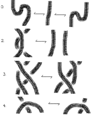 |
Move comprises the cancellation of adjacent maxima and minima. Move can be regarded as the cancellation of crossings of opposite type. Move is the basic braiding identity. Move is a “switchback” move that exchanges a crossing next to a maximum (minimum) for the maximum (minimum) next to the opposite crossing. Each of the moves can be regarded as a relation on the generating morphisms , , and . Specifically, here are the corresponding algebraic statements of these moves:
0. ,
2.
3.
4.
Each of these equations is taken in the context of the identifications and . The notation stands for the identity map on . This completes the description of the category
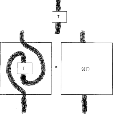
In discussing we shall continue to use the topological terminology tangle for a morphism in the category. An tangle is a tangle with inputs and outputs. Thus a tangle is any map from to in , and a tangle is any knot or link arranged with respect to the vertical to give a morphism from to . If is an tangle in we define to be the tangle obtained by replacing every strand of by two parallel copies of that strand. We leave it as an exercise for the reader to express on the generating morphisms. As we shall see, is an analog of the coproduct in a Hopf algebra. There is also an analog of the antipode in a Hopf algebra, defined in and taking an tangle to an tangle . The functor is defined by adding caps on the left and cups on the right of the tangle so that the inputs and outputs are reversed. See Figure 3 for an illustration of the tangle antipode . In we have where denotes the identity functor on tangles. This is a precursor to the special nature of the elements of the Hopf algebra category that will be the image of our functor from the tangle category to the Hopf algebra category.
 |
3.2 The Immersion Category
The Immersion Category, denoted Flat, is a quotient of the tangle category where we identify the maps and with each other. In this category, let denote the equivalence class of . The morphisms in are represented by tangle diagrams that are immersed in the plane (that is each curve in the diagram is the image of an immersion and distinct curves intersect transversely). The axioms for equivalence of morphisms in correspond to regular homotopy of flat tangles. The Whitney-Graustein Theorem [28] applies to this category. The Whitney-Graustein Theorem states that any immersed curve in the plane is regularly homotopic to a simple closed curve that is decorated with a string of curls, as indicated in Figure 4. A curl is a tangle in of the form or . The second curl is denoted by because the equations hold in as illustrated in Figure 5. These equations are the categorical analog of the so- called ”Whitney trick”. Whitney’s Theorem tells us that any flat tangle with a single strand is equivalent to an integer power of . The exponent is the Whitney degree of this curve, oriented from input to output. (The Whitney degree is the total turn of the tangent vector to the oriented curve. If the curve is a tangle then the Whitney degree of the identity tangle is zero. If the curve is a single strand tangle, then the Whitney degree depends upon the choice of orientation, with a clockwise oriented circle giving degree .
 |
 |
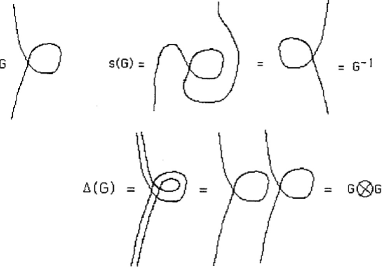
Note that in the morphism has the formal properties of a permutation of the factors of . For example . In computing the categorical antipode on the elements and , we find that and , as shown in Figure 6. This means that behaves as a formal group-like element in the category . Note also that , as shown in Figure 6.
 |
 |
3.3 The Category Arising From A Hopf Algebra
Let be an Hopf algebra. We shall define a category associated with this Hopf algebra. is a generalization of the immersion category . In the case where is quasi-triangular, we shall define a functor . The invariants described in the later sections of this paper are consequences of the existence of this functor.
The objects of are identical to the objects of , except that we take the abstract object and replace it by the ground ring of the Hopf algebra. Rather than make a separate notation for the distinction between as an abstract object and as the ground ring, we shall treat this contextually. Unless otherwise specified, a morphism from to is an abstract morphism, as in . Each element of is taken to be a morphism from to and the composition of elements and in is simply their product in . Similarly, each element of the tensor product of with itself is interpreted as a morphism from the -fold tensor product of to itself. Each element of the ground ring is interpreted as a morphism from to in the same way, except that now we can take this morphism as right multiplication by if we wish. The generating morphisms of consist in the morphisms of the tensor powers of (and ) together with the morphisms already available in . The relations on the morphisms in still hold, and we add the following interrelationships with the morphisms from the Hopf algebra:
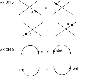
5. For and in (viewed as morphisms of to ),
6. For in , let denote the result of applying the antipode in to the element . Then
and
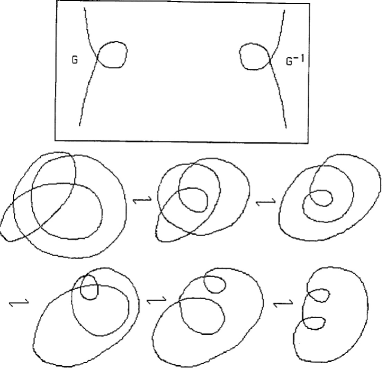
We have labeled these axioms and , since the category Cat(A) already partakes of the flat tangle axioms ,,, with the caveat that =. Note that says that does act as a permutation on morphisms coming from . See Figure 7 for an illustration of axioms 5 and 6.
There is one important addition to the structure of that is not included in the tangle categories. In we allow as morphisms formal sums of morphisms with coefficients in . Thus in extending to become a morphism in , we take the sum of the individual morphisms in this summation. A similar remark applies to the categorical interpretation of identities such as .
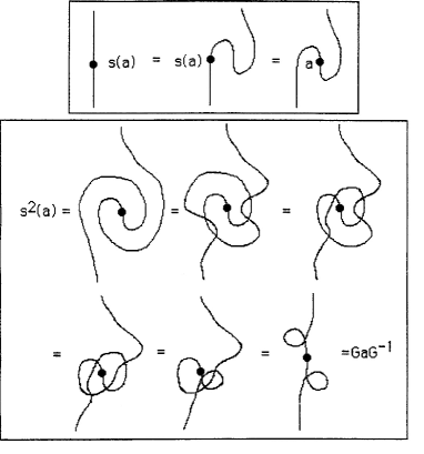
Axiom gives a direct relationship between the antipode in the Hopf algebra and the diagrammatic antipode that we described for the tangle category and flat tangle category. To see this relationship, we need to make a few remarks about the structure of the diagrams that represent morphisms in . A symbolic element of the Hopf algebra is diagrammed as a morphism in by taking a vertical line segment and labeling it with the letter next to a dot or ”bead” drawn on the line segment. We will refer to the location of the bead on a larger diagram. Thus, in axiom , corresponds to a drawing of the with a bead labeled on its right hand side (below the maximum), while corresponds to a drawing of the cap with a bead labeled on its left side. The equation gives us permission to “slide a bead counterclockwise around a maximum” while applying the antipode to it. Similarly, the other equation of says that we can slide a bead counterclockwise around a minimum and apply the antipode to that bead. Proofs by “sliding” can often replace algebraic manipulations. For example, in Figure 8 we illustrate a proof of the following lemma (standard proof given below) of the expression of the antipode in terms of cups and caps. Figure 8 also illustrates the interpretation of sliding beads across a permutation , and it gives a proof by sliding of the important formula
The square of the antipode (in ) is given by conjugation with the formal grouplike .
Lemma. Let be an element of viewed as a morphism from to . Then .
Proof.
 |
Let denote the set of all morphisms in from to that are supported on a single strand flat tangle. In other words, a morphism in consists of a single strand flat tangle that has been “decorated” with beads from at various spots that are neither maxima, minima or crossings in the strand. It is clear from our axioms that we can slide all the beads through the tangle until they are all encountered first along a straight piece of the strand. Thus, if is this morphism, then is equivalent to a product where is in and is a flat tangle free of elements of . By our work with , is equivalent to where is the flat curl and is the Whitney degree of . Thus is equivalent to . This means that, except for closed loops, the morphisms in are not much more than elements of the tensor powers of augmented by powers of the formal grouplike element .
It may not be apparent at first sight that the element in that we obtained from is uniquely determined by the equivalence class of in . (It is clear from our previous remarks that the Whitney degree of is determined by the equivalence class of .) In order to see this, we will give a definition of that is dependent only on the decomposition of as a product of cups, caps, permutations and elements of tensor products of the algebra . This is the same as saying that we will define in terms of a given diagrammatic representation of , since each diagrammatic representation is exactly a particular factorization of into elementary morphisms.
The algorithm for computing is as follows: Proceed upward along the strand of , creating two data structures. The first data structure is an element in whose initial value is . Let denote the generic form of this element of . The second data structure is a power of the antipode of whose initial value is the identity mapping. Let denote the generic form of this power of the antipode. Now, whenever you encounter a ”bead” on the strand, replace by . Whenever you move around a maximum or a minimum in a clockwise direction, replace by . Whenever you move around a maximum or a minimum in a counter-clockwise direction, replace by . The word is the word obtained by going from the bottom of the strand to the top of the strand by this process. The final value of will be , the Whitney degree of the tangle.
It is easy to see that is invariant under all the replacements generated by the axiom for the category , and it is equally easy to see that is exactly the element of that is obtained by sliding on a particular diagram. This shows that sliding is well-defined, and that the category does not lose any information that is present in the Hopf algebra . The Hopf algebra can be recovered from the morphisms of .
In the course of this discussion, we may have aroused the reader’s appetite for the the structure of the closed loop morphisms in . This will be taken up in the next section, when we discuss trace and integral. We are now ready to construct a functor from to when is quasi-triangular.
3.4 The Functor F:
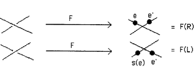
Let be a quasi-triangular Hopf algebra as described in Section 1. Let denote the Yang-Baxter element for and write symbolically in the form . We wish to define a functor from to . It suffices to define on the generating morphisms ,, and . We define
Diagrammatically, it is convenient to to picture as a flat crossing with beads above the crossing labeled and from left to right, with the summation indicated by the double appearance of the letter . Similarly, is depicted as a crossing with beads below the crossing and labeled and . See Figure 9.
 |
Recall the axioms ,, and for the tangle category.
0.
2.
3.
4.
In order for the functor to be well-defined, we must have the images of these relations satisfied in . For this, axiom follows at once since is taken to and to . Axiom follows directly since we designed as the inverse of . Axiom is exactly equivalent to the statement that satisfies the Yang-Baxter equation in . Thus we are left to verify
4.
This is verified by bead sliding in Figure 10.
 |
Knowing that is a functor on the tangle category, means that we have implicitly defined many invariants of knots and links, since regularly isotopic tangles will have equivalent images under . Before dealing with the intricacies of traces or of closed loops, we can state the following Theorem for 1-1 tangles, giving invariants with values in the Hopf algebra .
Theorem. Let be a single-stranded, 1-1 tangle. That is , is a “knot on a string”. Then is a regular isotopy invariant of . Here is the element of defined in the last section by concentrating all the algebra in in the lower part of the tangle, and is the Whitney degree of the plane curve underlying . In fact is itself a regular isotopy invariant of , as is .
Proof. This follows directly from the definition and well-definedness of the functor in conjunction with the discussion in the section on the category associated with a Hopf algebra.
Example. The curl obtained from by placing a crossing of type at its self-intersection maps, under , to the ribbon element when is a ribbon Hopf algebra. The factorization of v into the product is implicated by the slide convention for the antipode and the fact that See Figure 11.
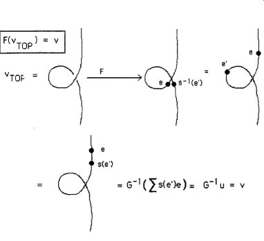 |
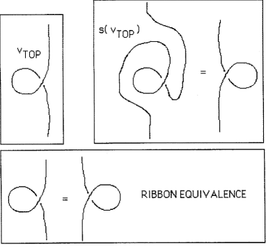
Remark. When the identification is added to regular isotopy, the twists catalog only the framing, and the equivalence relation on the link diagrams is the same as ambient isotopy of framed links. See Figure 12. We call this equivalence relation on link diagrams ribbon equivalence. Recall from Section 2 that a quasitriangular Hopf algebra is said to be a ribbon Hopf algebra if there exists a grouplike element such that is in the center of and where Note that algebraically, the condition is equivalent to the condition Thus Figures 11 and 12 show that a ribbon element is the exact counterpart of ribbon equivalence under the functor
 |
Remark. In general, if is a single strand tangle, and is the corresponding element in the quasitriangular Hopf algebra determined by our correspondence, then where the first is the diagrammatic coproduct and the second is the algebraic coproduct. This fact follows from the axioms for a quasitriangular Hopf algebra. In particular, we use axiom 2 from Section 2:
and the fact (a consequence of the axioms) that
when The naturality of the coproduct with respect to the functor is then a consequence of naturality with respect to the generating morphisms , , and as illustrated in Figure 13.
 |
4 Diagrammatic Geometry and the Trace
An augmented Hopf algebra is a Hopf algebra that contains a grouplike element such that for all in . We can adjoin such an element to any given Hopf algebra (See [10] for the details.). The result is an algebra in which the flat curl morphisms in can be identified with and . A ribbon Hopf algebra is an augmented quasi-triangular Hopf algebra with the extra properties that and is in the center of where is the Drinfeld element described in Section 2. It is useful to abstract the concept of augmented Hopf algebra when dealing with the category, , of a given Hopf algebra . We shall assume throughout this section that the Hopf algebra is augmented.
A function from the Hopf algebra to the base ring is said to be a trace if and for all and In this section we describe how a trace function on an augmented Hopf algebra yields an invariant, , of regular isotopy of knots and links.
Let denote the set of closed morphisms in from to . These morphisms are obtained from closed immersions of (collections) of circles that are decorated with elements of and arranged with respect to the vertical to form morphisms in from to . We would like to interpret such morphisms as actual mappings of the base ring to itself. In they are formal morphisms from to until further interpreted.
Define the right and left circle morphisms
and
by taking for in to the the morphism obtained from a circle (simple composition of and ) by placing on the right hand side of the circle. That is,
Similarly,
is the morphism that results from placing on the left hand side of the circle. Note that by our axioms for we have that (by sliding the bead around the circle).
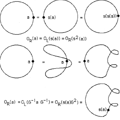
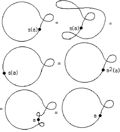
Here are some fundamental identities about these left and right circle morphisms.
These identities are proved diagrammatically in Figure 14. We will see that these identities are directly related to the formal structure of traces and integrals on a Hopf algebra.
 |
Slide Lemma. If is any single-component closed morphism in , then there is an element in such that . (Here equality denotes equality of morphisms in .)
Writing the tensor product of closed morphisms as juxtaposition, any n-component closed morphism has the form for some elements in . In this expression the summation sign denotes the possibility that there may be a summation over elements of that is shared among the components of the morphism.
Proof. By sliding, concentrate the algebra on the single-component morphism W into on a single segment of the immersion associated with . Now use the Whitney-Graustein Theorem to transform the immersion associated with W to a circle decorate with a product of curls. Translate the curls into a power of and amalgamate this with the algebra. The result is a circle decorated with an algebra element . Without loss of generality, we can assume that is on the right side of the circle. This shows that as desired. The multi-component statement follows by the same argument.
We can now point out a formal construction that has the properties of a trace. Define by the equation
Note that another way to describe is to say that the morphism is obtained by inscribing on a curve with vanishing Whitney degree (interpreting the in the definition of as a curl on the circle). This means that if is slid all the way around this curve it will return to its original position unchanged.
Lemma. With described as above,
for any and in
for any in .
Proof. by the remarks about sliding that precede the statement of this Lemma. Hence For the second part, (Alternatively, view Figure 15.) This completes the proof.
 |
Remark. Note that since , we have
and
This remark tells us that any closed single-component morphism can be expressed in terms of the formal trace . For, by the Slide Lemma above, we can write . Recall from the proof of the Slide Lemma that where is the element of that results from concentrating the algebra of to a single segment of . is the further concentration of curls at this segment that results from applying the Whitney-Graustein Theorem to the immersion for . If we then orient so that the selected segment has an upward arrow, then it is easy to see that is the Whitney degree of the immersion associated to . Thus have the
Evaluation Lemma. For any closed single-component morphism , where is the result of concentrating the algebra of on any segment of the immersion for and is the Whitney degree of this immersion, oriented so that the arrow is up at this segment. This formula for does not depend upon the choice of the segment where the concentration occurs. (The analogous result holds for a multi-component morphism. In this case, each closed loop can be dealt with separately as a formal trace, and there will usually be a summation over products of these traces.)
Proof. Most of the proof has already been given. Note that in concentrating the algebra, one may end up with on the left hand side of the circle. The relationship then shows that the same prescription works in this case. This completes the proof.
Definition. Two elements and of , are said to be slide equivalent if one can be obtained from the other by either globally applying the antipode or by rewriting the order of a product decomposition.
Thus and are slide equivalent and is slide equivalent to . (Note that is slide equivalent to but we make no assertion about the equivalence of and .) Thus, by the properties of the formal trace , we see that if is slide equivalent to , then . The next Lemma proves a converse to this statement.
Recovery Lemma. Let and be elements of . Then and are slide equivalent if and only if .
Proof. Recall that . Thus is obtained by decorating an immersion of Whitney degree zero with the algebra element . It is easy to see that slide equivalent elements in have the same image under . In fact, we have already formalized this fact by proving that and that . Since we can “forget” about the applications of the antipode to as is moved across a maximum or a minimum in any curve of total Whitney degree zero. That is, by our axioms that only way that can change in the course of equivalences to the morphism is by the application of the antipode to either all of or to some of its factors partially slid around the curve. Any time any factor is slid all the way around a curve it returns to its original value because the Whitney degree is zero. Then, since only slide equivalences are produced by regular homotopies of this immersion to itself, implies that and are slide equivalent. This completes the proof.
Remark. Suppose that is a trace function. That is, is a linear function satisfying
1. and
2.
Then it follows from the Recovery Lemma that we may define tr on single-component closed morphisms by the formula or where and the Whitney degree are obtained by concentrating the algebra on as in the Evaluation Lemma. This formula extends to products and multicomponent closed morphisms in that obvious way. The upshot is that a trace function on the Hopf algebra gives rise to an invariant of knots and links via our functor . This is discussed in the next section.
Definition and Computation of TR(K). Suppose that is a trace function. In order to define an invariant of unoriented links, concentrate the algebra for each component of the link, and define to be the sum of the products of the evaluations of the individual components of the link. It follows from our previous discussion that this will be a regular isotopy invariant of links.
Discussion. Note that invariants described according to the last definition can be regarded as computed either via the categorical decomposition of a morphism into cups, caps and crossings, or via the algebra concentration described in this section. In the categorical point of view, a diagram with no free ends is a morphism from to , where is the ground ring of the Hopf algebra. It is useful to have both points of view available both for theory and for computation.
5 Invariants of 3-manifolds
The structure we have built so far can be used to construct invariants of 3-manifolds presented in terms of surgery on framed links. We sketch here our technique that simplifies an approach to 3-manifold invariants of Mark Hennings [3].
Recall that an element of the dual algebra is said to be a right integral if for all in For a unimodular [16] ,[20] finite dimensional ribbon Hopf algebra there is a right integral satisfying the following properties for all x and y in A:
0) is unique up to scalar multiplication when is a field.
1)
2) where , the special grouplike element for the ribbon element
Given the existence of this integral , define a functional by the formula
(It follows from the fact that that )
It is then easy to prove the following theorem [8].
Trace Theorem. The function defined as above satisfies
for all in
and
for all in
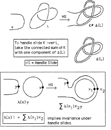
The upshot of this theorem is that for a unimodular finite dimensional Hopf algebra there is a natural trace defined via the existent right integral. Remarkably, this trace is just designed to behave well with respect to handle sliding [9] , [8]. Handle sliding is the basic transformation on framed links that leaves the corresponding 3-manifold obtained by framed surgery unchanged. See [12]. This means that a suitably normalized version of this trace on framed links gives an invariant of 3-manifolds. For a link , we let TR(K) denote the functional on links, as described in the previous section, defined via as above.
To see how the condition on handle sliding and the property of being a right integral are related in our category, we refer the reader to Figure 16 where the basic form of handle sliding is illustrated and its algebraic counterpart is shown. The algebraic counterpart arises when we concentrate all the algebra in a given link component in one place on the diagram. The component is then replaced by a circle and formally its evaluation is for a suitable in the Hopf algebra. As the diagram shows, if we let , then invariance under handle sliding is implicated by being a right integral on the Hopf algebra.
 |
A proper normalization of gives an invariant of the 3-manifold obtained by framed surgery on More precisely (assuming that and are non-zero), let
where denotes the number of components of K, and denotes the signature of the matrix of linking numbers of the components of (with framing numbers on the diagonal). Then is an invariant of the 3-manifold obtained by doing framed surgery on in the blackboard framing. This is our reconstruction of Hennings invariant [3] in an intrinsically unoriented context.
6 Centrality
In the body of this paper we have described the functor which assigns to each tangle a morphism in the category If we choose a trace for each closed component of the tangle, Section 4 tells us how to map the result of into the subcategory of in which all components are open (with a little care this second map, can be made into a functor). Finally, Section 3 describes how to map the result to an element of where is the number of open strands. This final quantity is a purely algebraic invariant of the tangle and is the primary object of interest. In particular, it assigns an element of to each 1-1 tangle. The range of this invariant is not all of (or all of in the case of 1-1 tangles) however, as we show in this section.
Notice that for the object in every element of can be thought of as the morphism from the object to itself (in particular, acts on as the morphism ). Thus the set of morphisms between two given objects and is an -bimodule, with acting on the left and right by left and right composition with the above morphism. Notice that the tensor product of morphisms is exactly the tensor product map of -bimodules. We say that a morphism is invariant if it commutes with the action, so that for all in (the adjoint action of on these morphisms can easily be defined in terms of this left and right action, and the definition of invariant says exactly that the morphism spans a trivial subrepresentation in the adjoint representation, the usual definition of an invariant element).
Action Theorem. The functor and the map from tangles to elements of which have no closed components, as described above, take tan gles to invariant elements of
Proof. To show that is invariant, since is a composition of cups, caps and morphisms of the form , –images of left and right crossings under the functor –it suffices to show that these morphisms commute with the action of . However the statement that and commute with this action is equivalent to the condition defining quasitriangularity. Finally, An identical argument applies to the , and so we conclude that
Now in general Section 3 tells us that can be written as where is a product of closed components (i.e. a morphism in ) and is an element of . Now since acts trivially on we have by the counit axiom that and and thus the invariance of implies the invariance of (if is nonzero). But will send to where is a product of one trace for each component, and thus to an invariant element. This concludes the proof.
A 1-1 tangle is a tangle with a single input strand and a single output strand. Then , and by our axioms for sliding algebra around cups and caps, is equivalent to the morphism corresponding to an algebra element of the form where is the special grouplike element that we have discussed in the previous sections. (The element is well-defined by sliding the algebra to the bottom of the tangle and evaluating the closed loops in the tangle by a given functorial trace.)
Centrality Theorem. The algebra element associated with a 1-1 tangle is in the center of the Hopf algebra .
Proof. By the Action Theorem we know that for all in Thus Hence is in the center of .
Remark. The argument that we have given to prove the centrality theorem may appear at first sight to be quite abstract. In fact, for each example one can trace through the steps in the argument and produce a corresponding algebraic derivation of the commutativity that the theorem implies. Each stage in the categorical argument (applying an identity relating couinit and antipode or counit and coproduct, commuting a coproduct with an R-matrix) corresponds to an algebraic identity on the word(s) obtained by sliding all the algebra to the bottom of the diagram (using our sliding conventions in the category). The fact that each closed component of the diagram is evaluated by a circle morphism means that the evaluations obtained after sliding the algebra on a given closed curve (to concentrate it in one segment) are independent of the location of the concentration.
A simple example (with no extra components) is illustrated in Figure 19. In this Figure the steps of the categorical proof are indicated, showing the successive locations of elements on the diagram. We can apply the functor to each of the diagrams in Figure 19, and then slide the algebra to the bottom of the diagram. Replacing the flat loops by or , we obtain an algebraic expression corresponding to each of the diagrams in the Figure. The algebraic expressions corresponding to each diagram in Figure 19 are listed below:
| (1) | |||||
| (2) | |||||
| (3) | |||||
| (4) | |||||
| (5) | |||||
| (6) |
Each line in this list is a direct translation from the corresponding diagram in Figure 19, and each successive line is algebraically equal to its predecessor. Note how the diagrams supply the right powers of the antipode and other details that empower the resulting algebraic demonstration. These same principles apply to all examples, including the case of extra components. We leave further examples as an exercise for the reader, but recommend the case of a single line encircled once by an unknotted circle. The corresponding algebraic expression is
where stands for the circle morphism that is applied to the extra component. The exercise is to prove that this element is in the center of the Hopf algebra by translating the categorical proof to an algebraic proof. In the next section we shall take up this theme of algebraic combinatorics again and show that our approach leads to other forms of algebraic proofs and to a deeper understanding of the nature of these central elements.
Remark. The reader should compare our treatment of centrality with [25]. This centrality proof is remarkable in that it uses the structure of the category, , to prove an essentially algebraic fact about . Of course it is in this category that tangles correspond to morphisms that are products of cups,caps and crossings. It is the structure of these building blocks that insures that tangles yield central elements in the algebra. To see the power of this argument, the reader should note that it proves that the ribbon element is in the center of the algebra, and that this in turn proves (via the categorical representation of the square of the antipode as conjugation by the grouplike element ) that the square of the antipode is represented by conjugation by the Drinfeld element . This proof that is quite different from the direct algebraic proof.
Remark. A natural question is whether there are elements of the center of the Hopf algebra which are not in the range of the functor applied to 1-1 tangles. In the cases of most interest, including the finite-dimensional quantum groups at roots of unity, the answer is no. These and many other cases where there is a Hennings-type invariant have the following property, referred to by Hennings as unimodularity: The morphism of corresponding to a full twist of two strands, corresponds via to an element of and therefore can be viewed as a map from to . Unimodularity means this map is nondegenerate. In particular, if is for some trace this map sends to the value of on the 1-1 tangle consisting of a single vertical strand encircled by a closed loop evaluated with By the preceding theorem, the resulting element of is in fact in the center. Thus we have a 1-1 map from traces to the image of It is shown in [22] that the space of traces on has the same dimension as the center of and thus that this map is actually onto the center. Thus we conclude that when the Hopf algebra is unimodular, maps 1-1 tangles onto the center. A subtler question is whether the image of single strand 1-1 tangles generates the center.
7 Centrality, Algebra and Combinatorics
It is puzzling that centrality is proved so smoothly using the categorical structure when it appears to be quite intricate at the level of pure algebra. The purpose of this section is to show how the computations appear at the algebra level and how this level is related to the combinatorics of link diagrams. In particular, we will finish the section with a new proof of centrality that confirms a longstanding conjecture of the first two authors of the paper. We conjectured that a certain algebraic method of moving an element across a sum of words would always result in a verification that for in the image of our functor. As we shall see, this method is directly related to the content of the categorical proof of centrality, and it has interesting combinatorial properties of its own.
Let denote the Yang-Baxter element for a quasi-triangular Hopf algebra Let denote the antipode of . In calculations below we follow the modified summation convention for indices. Thus will be simply denoted by Other examples of this usage are the formulas and
Note the following calculation:
Thus we have the identity
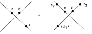 |
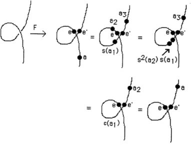
In Figure 17, we illustrate the diagram corresponding to this identity. This diagram suggests that we could “see” how a given element of the Hopf algebra is in the center by pushing beads on the diagram. For example, consider the following calculation with
This is exactly the sort of intricate algebraic argument that our categorical proof of centrality seems to avoid. Now view Figure 18. In Figure 18, we show that the above algebraic proof of centrality has an exact diagrammatic counterpart via the identity from Figure 17.
 |
Now view Figure 19. In this Figure we have illustrated the centrality of the same element as in Figure 18, but the diagrammatic proof follows the pattern of the Centrality Theorem of the last section. We see from this example that the proof of the Centrality Theorem actually does provide a sequence of algebraic steps that gives a specific proof of centrality for any given element of the Hopf algebra that is an image of a tangle under the functor . The algebraic proof that is so constructed is guided by the diagram of the tangle as it is arranged with respect to a vertical direction. The steps in the algebraic proof parallel the movement of the element across the sequence of morphisms into which is decomposed.
 |
We leave it to the reader to translate the diagrams of Figure 19 into an algebraic demonstration. The point is that once a given diagram is chosen, then the steps of moving elements across the elementary morphisms are exactly specified and each step in this process yields an algebraic step that can be verified by the usual means.
We now show that the method corresponding to Figures 17 and 18 will always work to provide proofs of centrality. In this method, we generalize the formula in Figure 17 to all the different cases of a bead at one of the legs of a crossing. It is easy to verify that the resulting patterns do not depend upon the crossing type. The exact result is given in the next Lemma, whose proof we omit. See Figure 20 for the pattern of diagrammatic bead slides. In this figure the crossings are indicated with a dark vertex that can be either an undercrossing or an overcrossing. Note that if the bead has an antipode applied to it, then the order of indices will shift from clockwise around the crossing to anticlockwise around the crossing (or vice-versa). With the help of the diagrams in Figure 20 one can experiment on link diagrams and produce proofs of centrality by direct bead pushing as we did in Figure 17. View Figures 21 for an example of this procedure.
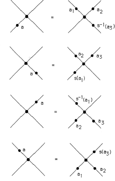 |
Bead Push Lemma. Let denote the Yang-Baxter element for a quasi-triangular Hopf algebra Let denote the antipode of . (In the following formulas will be denoted by )
1.
2.
3.
4.
5.
6.
7.
8.
Proof. Omitted.
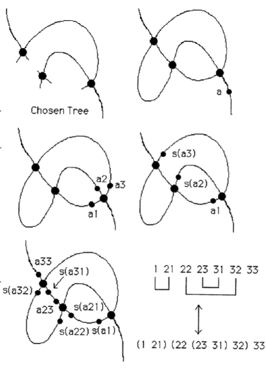 |
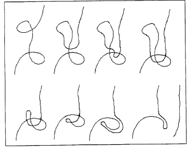
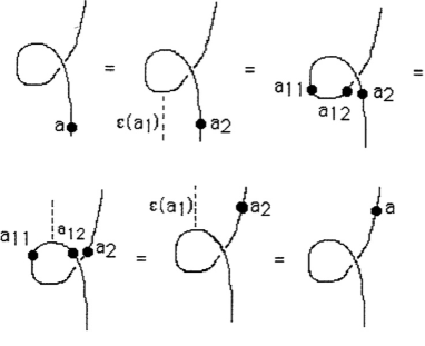
In Figure 21 we illustrate one way to verify centrality for a trefoil tangle via bead pushing (here illustrated without crossing choices since the patterns of bead pushing do not depend upon the choice of crossing). In this procedure, we choose a connected tree that is obtained from the tangle for the trefoil by cutting midpoints of an appropriate subset of the edges of the projected flat tangle. Once this tree is chosen, there is a unique way to push a bead (labeled ) from the lower leg of the tangle to all the branches of the tree including the upper tangle leg. Except for the upper and lower legs of the tangle all the twigs of the tree are paired by the cutting arcs. We see in this example that each pair of paired twigs gives rise to a “cancellation” of the form and “reconstruction” in the form . These cancellations occur in sequence via the lexicographic ordering corresponding to the particular splitting into coproducts that is dictated by the tree. Thus in the case of Figure 21 we have the ordering
The parentheses indicate the pairings. Thus and are paired; and are paired; and are paired. If and are paired then we set a left parenthesis before and a right parenthesis after in the lexicographic ordering. In the Figure 21 we have replaced the parentheses by connecting arcs. Now note that the parentheses so obtained are nested in the classical fashion of well-formed parentheses. A cancellation of then leads to a cancellation of and there is a parallel cancellation of In the end we are left with reconstructed at the top edge of the tangle and hence a proof of centrality for this particular tangle.
We now wish to show that the example in Figure 21 is quite general and that this procedure will work on any tangle. In order to accomplish this end it must be shown that
1. For any choice of tree in a tangle , each pair of paired beads will have powers of the antipode applied to them that differ by one when they are moved into the same vertical sector of a common edge (See Figure 18 for an example.).
2. The lexicographic order of coproducts combined with the pairings gives rise to a well-formed structure of parentheses (so that the cancellation and reconstruction can proceed).
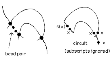
Condition 1 is proved by noting that paired beads are part of a circuit in the tangle, as illustrated in Figure 22. The (Figure 20) rules for bead pushing make it easy to see that the total exponent for going around this circuit is the same as its Whitney degree(namely plus or minus one) just as we discussed in earlier sections. The key observation (available directly from Figure 20) is that the pattern of application of the antipode in the bead push is exactly the same as if the crossing were smoothed horizontally or vertically and the bead was pushed (possibly across a maximum or a minimum) according to the rules of our category).
 |
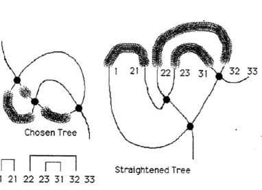 |
Condition 2 is proved by first noting (via the Bead Push Lemma) that the lexicographic ordering and pairings for a given choice of tangle diagram and tree is the same as the lexicographic ordering and pairings in the new diagram obtained by straightening the tree by a planar isotopy so that each push moves upwards (with respect to the chosen vertical direction) and there are no maxima in the arcs of the tree. In this case each vertex in the tree gives a clockwise ordering as dictated by the Bead Push Lemma and Figure 20. In Figure 23 we illustrate this isotopy and the resulting ordering. The reader should compare this ordering with the ordering in Figure 21. Once the tree is straightened, it is clear that the well-formedness of the parenthesis structure corresponds to the fact that the arcs connecting paired beads (each such arc is now a maximum with respect to the vertical) do not intersect one another. The well-formed parentheses are a direct consequence of the planarity of the graph of the flat tangle.
This completes the proof that bead pushing into the twigs of a tree will always prove centrality for tangles. The reader should note that these arguments apply to tangles with multiple components just so long as the circle morphisms for closed components take values in the ground ring (See Section 4.). We have spent the effort to relate bead pushing with centrality because the result is intriguing and because it shows quite clearly the relationship between centrality in the Hopf algebra and the combinatorics of plane graphs and trees.
It remains to be seen if these methods can be inverted to give a complete characterisation of central elements in quasi-triangular Hopf algebras (i.e. elements that correspond to the image of 1-1 tangles under our functor from tangles to the category associated with a Hopf algebra).
It is worth remarking that the result we have described is invertible at the formal level in the following sense: If we know how to thread (that is prove ) an arbitrary element of the Hopf algebra through a given sum of words where as a summation has the structure of a sum over repeated Yang-Baxter elements, and if this threading involves only applications of the bead push identities and the counit and antipode identities (as in our discussion), then the threading will, of its own accord, produce a tree with a lexicographic ordering of the branches and a legal parenthetical association of these branches. This data gives an embedding of the tree and parenthesis arcs into the plane. That planar embedding specifies a link diagram whose image is under our functor.
A Quantum Remark. One can interpret the “beads” moving on the tangle diagrams as ”particles” that scatter through a “spin network” that corresponds to the given tangle. In this interpretation, each element of the Hopf algebra (seen as a morphism in ) is a quantum particle traveling forward in time. The application of the antipode, is interpreted as “ traveling backwards in time.” The identity is interpreted as the emission or absorption by of a “virtual photon”. Note that when the virtual photon is present, then is in a mixed state connoted by the summation over and . The identity corresponds to the creation or annihilation of a particle and an antiparticle. (Note that grammatically it is not “a particle and an antiparticle” but rather a “particle/antiparticle mixed state”. Then our result on centrality is interpreted by saying that the tangle is a “self-energy diagram” in which the particle undergoes a virtual interaction that returns it to its original state.
8 Applications to Virtual Knot Theory
The categorical methods in this paper can be applied to virtual knot theory. The flat crossings of the category of a Hopf algebra have the same formal properties as the virtual crossings
in rotational virtual knot theory. See [5] for a detailed explanation of rotational virtual knot theory and the construction of the generalization of the methods of this paper for that category.
In defining a functor on the virtual tangle category one takes the virtual crossing in a tangle diagram to a flat crossing
in the Hopf algebra category. Another possible application to virtual knots for the three manifold invariants in this paper can be investigated via the virtual three manifolds, Kirby calculus and invariants of three manifolds as constructed in [2]. This application to invariants of virtual three-manifolds will be the subject of a further paper.
References
- [1] V.G. Drinfeld, Quantum groups. Proceedings of the International Congress of Mathematicians, Berkeley, California, USA(1987), 798- 820.
- [2] H. A. Dye and L. H. Kauffman, Virtual knot diagrams and the Witten-Reshetikhin-Turaev invariant. J. Knot Theory Ramifications 14 (2005), no. 8, 1045 1075.
- [3] M.A.Hennings, Invariants of links and 3-manifolds obtained from Hopf algebras. (preprint 1989)
- [4] L. H. Kauffman, D. Radford, S. Sawin, Centrality and the KRH Invariant, Journal of Knot Theory and Its Ramifications, Vol. 7, No. 5 (1998) 571-624, World Scientific Pub
- [5] L. H. Kauffman, Rotational virtual knots and quantum link invariants. J. Knot Theory Ramifications 24 (2015), no. 13, 1541008, 46 pp.
- [6] L.H. Kauffman, Knots and Physics. World Sci. Pub. (1991,1994,2012).
- [7] L.H. Kauffman and D.E. Radford, A necessary and sufficient condition for a finite- dimensional Drinfel’d double to be a ribbon Hopf algebra. Journal of Algebra, Vol. 159, No. 1, pp. 98 -114.
- [8] L.H. Kauffman and D.E. Radford, Invariants of 3- manifolds derived from finite dimensional Hopf algebras. Journal of Knot Theory and Its Ramifications, Vol. 4, No. 1 (1995), 131-162.
- [9] L. H. Kauffman, Hopf algebras and invariants of 3-manifolds. Journal of Pure and Applied Algebra, Vol. 100 (1995) 73-92.
- [10] L. H. Kauffman and D. E. Radford, Quantum algebras, quantum coalgebras, invariants of tangles and knots. Comm. Algebra 28 (2000), no. 11, 5101–5156.
- [11] T. Kerler, Mapping Class Group Actions on Quantum Doubles. Comm. Math. Phys. 168 (1995), no. 2, 353 388.
- [12] R. Kirby, A calculus for framed links in Invent. Math. Vol. 45 (1978),35-56.
- [13] R. Kirby and P. Melvin, The 3-manifold invariants of Witten and Reshetikhin- Turaev for Invent. Math. Vol. 105, 473-545 (1991).
- [14] G. Kuperberg, Involutory Hopf algebras and 3-manifold invariants, Int. J. of Math. (1991), 41-66.
- [15] G. Kuperberg, Noninvolutory Hopf algebras and 3-manifold invariants. Duke Math. J. 84 (1996), no. 1, 83 129.
- [16] R.G. Larson and M.E. Sweedler, An associative orthogonal bilinear form for Hopf algebras. Amer. J. Math.Vol. 91 (1969), 75-94.
- [17] R.J. Lawrence, A universal link invariant using quantum groups. Differential Geometric Methods in Theoretical Physics, Chester(1988), 55-63.
- [18] V. Lyubashenko, Invariants of 3-manifolds and projective representations of mapping class groups via quantum groups at roots of unity. (English summary) Comm. Math. Phys. 172 (1995), no. 3, 467 516.
- [19] T. Ohtsuki, Invariants of 3-manifolds derived from universal invariants of framed links. Math. Proc. Cambridge Philos. Soc. 117 (1995), no. 2, 259 273.
- [20] D.E. Radford, The trace function and Hopf algebras. Journal of Algebra, Vol 163, No. 3, February 1, (1994), 583 - 622.
- [21] D.E. Radford, Generalized double crossproducts associated with the quantized enveloping algebras. Comm. Algebra 26 (1998), no. 1, 241 291.
- [22] D.E. Radford, On Kauffman’s knot invariants arising from finite-dimensional Hopf algebras. Advances in Hopf algebras (Chicago, IL, 1992), 205 266, Lecture Notes in Pure and Appl. Math., 158, Dekker, New York, 1994.
- [23] K. Reidemeister, Knotentheorie. Chelsea Pub. Co., N.Y. (1948), Copyright 1932, Julius Springer, Berlin.
- [24] N. Yu. Reshetikhin and V.G. Turaev, Ribbon graphs and their invariants derived from quantum groups. Commun. Math. Phys. Vol. 127 (1990) 1-26.
- [25] N. Yu. Reshetikhin, Quasitriangular Hopf Algebras and Invariants of Tangles. Leningrad Math. J. Vol.1 No. 2, (1990),491- 513.
- [26] N. Yu. Reshetikhin and V. G. Turaev, Invariants of 3-manifolds via link polynomials and quantum groups. Invent. Math. Vol. 103 (1991), 547- 597.
- [27] M.E. Sweedler, Hopf Algebras. Mathematics Lecture Notes Series, Benjamin, New York, 1969.
- [28] H. Whitney, On regular closed curves in the plane. Comp. Math., (1937), 276-284.
- [29] E. Witten, Quantum field theory and the Jones polynomial. Commun. Math. Phys. Vol. 121 (1989), 351-399.