Bilinear Scoring Function Search
for Knowledge Graph Learning

Abstract

Learning embeddings for entities and relations in knowledge graph (KG) have benefited many downstream tasks. In recent years, scoring functions, the crux of KG learning, have been human designed to measure the plausibility of triples and capture different kinds of relations in KGs. However, as relations exhibit intricate patterns that are hard to infer before training, none of them consistently perform the best on benchmark tasks. In this paper, inspired by the recent success of automated machine learning (AutoML), we search bilinear scoring functions for different KG tasks through the AutoML techniques. However, it is non-trivial to explore domain-specific information here. We first set up a search space for AutoBLM by analyzing existing scoring functions. Then, we propose a progressive algorithm (AutoBLM) and an evolutionary algorithm (AutoBLM+), which are further accelerated by filter and predictor to deal with the domain-specific properties for KG learning. Finally, we perform extensive experiments on benchmarks in KG completion, multi-hop query, and entity classification tasks. Empirical results show that the searched scoring functions are KG dependent, new to the literature, and outperform the existing scoring functions. AutoBLM+ is better than AutoBLM as the evolutionary algorithm can flexibly explore better structures in the same budget.

1 Introduction

The knowledge graph (KG) [1, 2, 3] is a graph in which the nodes represent entities, the edges are the relations between entities, and the facts are represented by triples of the form (head entity, relation, tail entity) (or $(h,r,t)$ in short). The KG has been found useful in a lot of data mining and machine learning applications and tasks, including question answering [4], product recommendation [5], knowledge graph completion [6, 7], multi-hop query [8, 4], and entity classification [9].

In a KG, plausibility of a fact $(h,r,t)$ is given by $f(h,r,t)$, where $f$ is the scoring function. Existing $f$’s are custom-designed by human experts, and can be categorized into the following three families: (i) translational distance models (TDMs) [10, 11, 12, 13], which model the relation embeddings as translations from the head entity embedding to the tail entity embedding; (ii) bilinear model (BLMs) [6, 7, 14, 15, 16, 17, 18, 19], which model the interaction between entities and relations by a bilinear product between the entity and relation embeddings; and (iii) neural network models (NNMs) [20, 21, 22, 23, 24], which use neural networks to capture the interaction. The scoring function can significantly impact KG learning performance [2, 3, 25]. Most TDMs are less expressive and have poor empirical performance [3, 26]. NNMs are powerful but have large numbers of parameters and may overfit the training triples. In comparison, BLMs are more advantageous in that they are easily customized to be expressive, have linear complexities w.r.t. the numbers of entities/relations/dimensions, and have state-of-the-art performance [18]. While a number of BLMs have been proposed, the best BLM is often dataset-specific.

Recently, automated machine learning (AutoML) [27, 28] has demonstrated its power in many machine learning tasks such as hyperparameter optimization (HPO) [29] and neural architecture search (NAS) [30, 31, 32]. The models discovered have better performance than those designed by humans, and the amount of human effort required is significantly reduced. Inspired by its success, we propose in this paper the use of AutoML for the design of KG-dependent scoring functions. To achieve this, one has to pay careful consideration to the three main components in an AutoML algorithm: (i) search space, which identifies important properties of the learning models to search; (ii) search algorithm, which ensures that finding a good model in this space is efficient; and (iii) evaluation method, which offers feedbacks to the search algorithm.

In this paper, we make the following contributions in achieving these goals:

• We design a search space of scoring functions, which includes all the existing BLMs. We further analyze properties of this search space, and provide conditions for a candidate scoring function to be expressive, degenerate, and equivalent to another.

• To explore the above search space properties and reduce the computation cost in evaluation, we design a filter to remove degenerate and equivalent structures, and a performance predictor with specifically-designed symmetry-related features (SRF) to select promising structures.

• We customize a progressive algorithm (AutoBLM) and an evolutionary algorithm (AutoBLM+) that, together with the filter and performance predictor, allow flexible exploration of new BLMs.

Extensive experiments are performed on the tasks of KG completion, multi-hop query and entity classification. The results demonstrate that the models obtained by AutoBLM and AutoBLM+ outperform the start-of-the-art human-designed scoring functions. In addition, we show that the customized progressive and evolutionary algorithms are much less expensive than popular search algorithms (random search, Bayesian optimization and reinforcement learning) in finding a good scoring function.

Differences with the Conference Version. Compared to the preliminary version published in ICDE 2020 [33], we have made the following important extensions:

1. Theory. We add new analysis to the designed search space based on bilinear models. We theoretically prove when the candidates in the search space can be expressive (Section 3.2), degenerate (Section 3.4.1) and equivalent structures (Section 3.4.2).

2. Algorithm. We extend the search algorithm with the evolutionary algorithm (Section 4.4), i.e., AutoBLM+. The evolutionary strategy in Algorithm 4 can explore better in the search space, and can also leverage the filter and predictor to deal with the domain-specific properties.

3. Tasks. We extend AutoBLM and AutoBLM+ to two new tasks, namely, multi-hop query (Section 5.2) and entity classification in (Section 5.3). We show that the search problem can be well adopted to these new scenarios, and achieve good empirical performance.

4. Ablation Study. We conduct more experiments on the performance (Section 5.1.2 and 5.1.3) and analysis (Section 5.1.4) of the new search algorithm, analysis on the influence of $K$ (Section 5.1.7), and the problem of parameter sharing (Section 5.1.8) to analyze the design schemes in the search space and search algorithm.

Notations. In this paper, vectors are denoted by lowercase boldface, and matrix by uppercase boldface. The important notations are listed in Table I.

TABLE I: Notations used in the paper.

$\mathcal{E},\mathcal{R},\mathcal{S}$	set of entities, relations, triples
$|\mathcal{E}|,|\mathcal{R}|,|\mathcal{S}|$	number of entities, relations, triples
$(h,r,t)$	triple of head entity, relation and tail entity
$\bm{h},\bm{r},\bm{t}$	embeddings of $h$, $r$, and $t$
$f(h,r,t)$	scoring function for triple $(h,r,t)$
$\mathbb{R}^{d},\mathbb{C}^{d},\mathbb{H}^{d}$	$\!\!d$-dimensional real/complex/hypercomplex space
$\bm{R}_{(\bm{r})}\!\in\!\mathbb{R}^{d\times d}$	square matrix based on relation embedding $\bm{r}$
$\langle\bm{a},\bm{b},\bm{c}\rangle$	triple product $:=\sum_{i=1}^{d}a_{i}b_{i}c_{i}=\bm{a}^{\top}\text{diag}\!\left(\bm{b}\right)\bm{c}$
$\|\bm{v}\|_{1}$	$\ell_{1}$-norm of vector $\bm{v}$
$\text{Re}(\bm{v})$	real part of complex vector $\bm{v}\in\mathbb{C}^{d}$
$\bar{\bm{v}}$	conjugate of complex vector $\bm{v}\in\mathbb{C}^{d}$

2 Background and Related Works

2.1 Scoring Functions for Knowledge Graph (KG)

A knowledge graph (KG) can be represented by a third-order tensor $\mathbf{G}\in\mathbb{R}^{|\mathcal{E}|\times|\mathcal{R}|\times|\mathcal{E}|}$, in which $G_{hrt}=1$ if the corresponding triple $(h,r,t)$ exists in the KG, and 0 otherwise. The scoring function $f(h,r,t):\mathcal{E}\times\mathcal{R}\times\mathcal{E}\rightarrow\mathbb{R}$ measures plausibility of the triple $(h,r,t)$. As introduced in Section 1, it is desirable for a scoring function to be able to represent any of the symmetric, anti-symmetric, general asymmetric and inverse KG relations in Table II.

TABLE II: Popular properties in KG relations.

property	examples in WN18/FB15k	constraint on $f$
symmetry	isSimilarTo, spouseOf	$f(t,r,h)\!=\!f(h,r,t)$
anti-symmetry	ancestorOf, isPartOf	$f(t,r,h)\!=\!-f(h,r,t)$
general asymmetry	locatedIn, profession	$f(t,r,h)\!\neq\!f(h,r,t)$
inverse	hypernym, hyponym	$f(t,r,h)\!=\!f(h,r^{\prime},t)$

Definition 1 (Expressiveness [14, 34, 35]).

A scoring function is fully expressive if for any KG $G$ and the corresponding tensor $\mathbf{G}\in\mathbb{R}^{|\mathcal{E}|\times|\mathcal{R}|\times|\mathcal{E}|}$, one can find an instantiation $f$ of the scoring function such that $f(h,r,t)=G_{hrt}$, $\forall h,t\in\mathcal{E},r\in\mathcal{R}$.

Not all scoring functions are fully expressive. For example, consider a KG with two people A, B, and a relation “OlderThan”. Obviously, we can have either (A, OlderThan, B) or (B, OlderThan, A), but not both. The scoring function $f(h,r,t)=\langle\bm{h},\bm{r},\bm{t}\rangle=\sum_{i=1}^{d}h_{i}r_{i}t_{i}$, where $\bm{h},\bm{r},\bm{t}$ are $d$-dimensional embeddings of $h,r$ and $t$, respectively, cannot be fully expressive since $f(h,r,t)=f(t,r,h)$.

On the other hand, while expressiveness indicates the ability of $f$ to fit a given KG, it may not generalize well when inference on different KGs. As real-world KGs can be very sparse [1, 3], a scoring function with a large amount of trainable parameters may overfit the training triples. Hence, it is also desirable that the scoring function has only a manageable number of parameters.

In the following, we review the three main types of scoring functions, namely, translational distance model (TDM), neural network model (NNM), and biLinear model (BLM). As will be seen, many TDMs (such as TransE [10] and TransH [11]) cannot model the symmetric relations well [3, 36]. Neural network models, though fully expressive, have large numbers of parameters. This not only prevents the model from generalizing well on unobserved triples in a sparse KG, but also increases the training and inference costs [21, 18, 24]. In comparison, BLMs (except DistMult) can model all relation pattens in Table II and are fully expressive. Besides, these models (except RESCAL and TuckER) have moderate complexities (with the number of parameters linear in $|\mathcal{E}|,|\mathcal{R}|$ and $d$). Therefore, we consider BLM as a better choice, and it will be our focus in this paper.

TABLE III: The representative BLM scoring functions. For each scoring function we show the definitions, expressiveness in Definition 1, the ability to model all common relation patterns in Table II (“RP” for short), and the number of parameters.

scoring function	definition	expressiveness	RP	# parameters
RESCAL [6]	$\bm{h}^{\top}\bm{R}_{(\bm{r})}\bm{t}$	$\surd$	$\surd$	$O\left(|\mathcal{E}|d+|\mathcal{R}|d^{2}\right)$
DistMult [7]	$\langle\bm{h},\bm{r},\bm{t}\rangle$	$\times$	$\times$	$O(|\mathcal{E}|d+|\mathcal{R}|d)$
ComplEx [14]/HolE [15]	Re$\left({\bm{h}}\otimes{\bm{r}}\otimes\bar{{\bm{t}}}\right)$	$\surd$	$\surd$	$O\left(|\mathcal{E}|d+|\mathcal{R}|d\right)$
Analogy [16]	$\langle\hat{\bm{h}},\hat{\bm{r}},\hat{\bm{t}}\rangle$ + Re$\left(\underline{\bm{h}}\otimes\underline{\bm{r}}\otimes\bar{\underline{\bm{t}}}\right)$	$\surd$	$\surd$	$O\left(|\mathcal{E}|d+|\mathcal{R}|d\right)$
SimplE [17]/CP [18]	$\langle\hat{\bm{h}},\hat{\bm{r}},\underline{\bm{t}}\rangle$ + $\langle\underline{\bm{h}},\underline{\bm{r}},\hat{\bm{t}}\rangle$	$\surd$	$\surd$	$O\left(|\mathcal{E}|d+|\mathcal{R}|d\right)$
QuatE [19]	$\bm{h}\odot\bm{r}\odot\bm{t}$	$\surd$	$\surd$	$O\left(|\mathcal{E}|d+|\mathcal{R}|d\right)$
TuckER [35]	$\mathcal{W}\times_{1}\bm{h}\times_{2}\bm{r}\times_{3}\bm{t}$	$\surd$	$\surd$	$O\left(|\mathcal{E}|d+|\mathcal{R}|d+d^{3}\right)$

Translational Distance Model (TDM). Inspired by analogy results in word embeddings [37], scoring functions in TDM take the relation $r$ as a translation from $h$ to $t$. The most representative TDM is TransE [10], with $f(h,r,t)=-\|\bm{t}-(\bm{h}+\bm{r})\|_{1}$. In order to handle one-to-many, many-to-one and many-to-many relations, TransH [11] and TransR [12] introduce additional vectors/matrices to map the entities to a relation-specific hyperplane. The more recent RotatE [13] treats the relations as rotations in a complex-valued space: $f(h,r,t)=-\|\bm{t}-\bm{h}\otimes\bm{r}\|_{1}$, where $\bm{h},\bm{r},\bm{t}\in\mathbb{C}^{d}$ and $\otimes$ is the Hermitian product [14]. As discussed in [34], most TDMs are not fully expressive. For example, TransE and TransH cannot model symmetric relations.

Neural Network Model (NNM). NNMs take the entity and relation embeddings as input, and output a probability for the triple $(h,r,t)$ using a neural network. Earlier works are based on multilayer perceptrons [20] and neural tensor networks [38]. More recently, ConvE [21] uses the convolutional network to capture interactions among embedding dimensions. By sampling relational paths [39] from the KG, RSN [22] and Interstellar [40] use the recurrent network [41] to recurrently combine the head entity and relation with a step-wise scoring function. As the KG is a graph, R-GCN [23] and CompGCN [24] use the graph convolution network [9] to aggregate entity-relation compositions layer by layer. Representations at the final layer are then used to compute the scores. Because of the use of an additional neural network, NNM requires more parameters and has larger model complexity.

BiLinear Model (BLM). BLMs model the KG relation as a bilinear product between entity embeddings. For example, RESCAL [6] defines $f$ as: $f(h,r,t)=\bm{h}^{\top}\bm{R}_{(\bm{r})}\bm{t}$, where $\bm{h},\bm{t}\in\mathbb{R}^{d}$, and $\bm{R}_{(\bm{r})}\in\mathbb{R}^{d\times d}$. To avoid overfitting, DistMult [7] requires $\bm{R}_{(\bm{r})}$ to be diagonal, and $f(h,r,t)$ reduces to a triple product: $f(h,r,t)=\bm{h}^{\top}\text{diag}\!\left(\bm{r}\right)\bm{t}=\left\langle\bm{h},\bm{r},\bm{t}\right\rangle$. However, it can only model symmetric relations. To capture anti-symmetric relations, ComplEx [14] uses complex-valued embeddings $\bm{h},\bm{r},\bm{t}\in\mathbb{C}^{d}$ with $f(h,r,t)=\text{Re}\big{(}\bm{h}^{\top}\text{diag}\!\left(\bm{r}\right)\bar{\bm{t}}\big{)}=\text{Re}\left(\bm{h}\otimes\bm{r}\otimes\bar{\bm{t}}\right)$, where $\otimes$ is the Hermitian product in complex space [14]. HolE [15] uses the circular correlation instead of the dot product, but is shown to be equivalent to ComplEx [42].

Analogy [16] decomposes the head embedding $\bm{h}$ into a real part $\hat{\bm{h}}\in\mathbb{R}^{\hat{d}}$ and a complex part $\underline{\bm{h}}\in\mathbb{C}^{\underline{d}}$. Relation embedding $\bm{r}$ (resp. tail embedding $\bm{t}$) is similarly decomposed into a real part $\hat{\bm{r}}$ (resp. $\hat{\bm{t}}$) and a complex part $\underline{\bm{r}}$ (resp. $\underline{\bm{t}}$). $f$ is then written as: $f(h,r,t)=\langle\hat{\bm{h}},\hat{\bm{r}},\hat{\bm{t}}\rangle+\text{Re}\big{(}\underline{\bm{h}}\otimes\underline{\bm{r}}\otimes\bar{\underline{\bm{t}}}\big{)}$, which can be regarded as a combination of DistMult and ComplEx. To simultaneously model the forward triplet $(h,r,t)$ and its inverse $(t,r^{\prime},h)$, SimplE [17] / CP [18] similarly splits the embeddings to a forward part ($\hat{\bm{h}},\hat{\bm{r}},\hat{\bm{t}}\in\mathbb{R}^{d}$) and a backward part ($\underline{\bm{h}},\underline{\bm{r}},\underline{\bm{t}}\in\mathbb{R}^{d}$): $f(h,r,t)=\langle\hat{\bm{h}},\hat{\bm{r}},\underline{\bm{t}}\rangle+\langle\underline{\bm{t}},\underline{\bm{r}},\hat{\bm{h}}\rangle$. To allow more interactions among embedding dimensions, the recent QuatE [19] uses embeddings in the hypercomplex space ($\bm{h},\bm{r},\bm{t}\in\mathbb{H}^{d}$) to model $f(h,r,t)=\bm{h}\odot\bm{r}\odot\bm{t}$ where $\odot$ is the Hamilton product. By using the Tucker decomposition [43], TuckER [35] proposes a generalized bilinear model and introduces more parameters in the core tensor $\mathcal{W}\in\mathbb{R}^{d\times d\times d}$: $f(h,r,t)=\mathcal{W}\times_{1}\bm{h}\times_{2}\bm{r}\times_{3}\bm{t}$, where $\times_{i}$ is the tensor product along the $i$th mode. A summary of these BLMs is in Table III.

2.2 Common Learning Tasks in KG

2.2.1 KG Completion

KG is naturally incomplete [1], and KG completion is a representative task in KG learning [3, 6, 10, 17, 14, 7, 21]. Scores on the observed triples are maximized, while those on the non-observed triplets are minimized. After training, new triples can be added to the KG by entity prediction with either a missing head entity $(?,r,t)$ or a missing tail entity $(h,r,?)$ [3]. For each kind of query, we enumerate all the entities $e\in\mathcal{E}$ and compute the corresponding scores $f(e,r,t)$ or $f(h,r,e)$. Entities with larger scores are more likely to be true facts. Most of the models in Section 2.1 can be directly used for KG completion.

2.2.2 Multi-hop Query

In KG completion, we predict queries $(h,r,?)$ with length one, i.e., $1$-hop query. In practice, there can be multi-hop queries with lengths larger than one [39, 8, 3]. For example, one may want to predict “who is the sister of Tony’s mother”. To solve this problem, we need to solve the length-2 query problem $(?,sister\circ mother,Tony)$ with the relation composition operator $\circ$.

Given the KG $\mathcal{G}=\{\mathcal{E},\mathcal{R},\mathcal{S}\}$, let $\varphi_{r}$, corresponding to the relation $r\in\mathcal{R}$, be a binary function $\mathcal{E}\times\mathcal{E}\mapsto\{True,False\}$. The multi-hop query is defined as follows.

Definition 2 (Multi-hop query [8, 4]).

The multi-hop query $(e_{0},r_{1}\circ r_{2}\circ\dots\circ r_{L},e_{?})$ with length $L>1$ is defined as $\exists e_{1}\dots e_{L-1},e_{?}:\varphi_{\!r_{1}}(e_{0},e_{1})\!\wedge\!\varphi_{\!r_{2}}(e_{1},e_{2})\!\wedge\!\dots\!\wedge\!\varphi_{\!r_{L}}(e_{L-1},e_{?})$ where $\wedge$ is the conjunction operation, $e_{0}$ is the starting entity, $e_{?}$ is the entity to predict, and $e_{1}\dots e_{L-1}$ are intermediate entities that connect the conjunctions.

Similar to KG completion, plausibility of a query $(e_{0},r_{1}\circ r_{2}\circ\dots\circ r_{L},e_{L})$ is measured by a scoring function [39, 8]:

$$f(e_{0},r_{1}\circ r_{2}\circ\dots\circ r_{L},e_{L})=\bm{e}_{0}^{\top}\bm{R}_{(r_{1})}\cdots\bm{R}_{(r_{L})}\bm{e}_{L},$$ (1)

where $\bm{R}_{(r_{i})}$ is a relation-specific matrix of the $i$th relation. The key is on how to model the composition of relations in the embedding space. Based on TransE [10], TransE-Comp [39] models the composition operator as addition, and defines the scoring function as $f(e_{0},r_{1}\circ\cdots\circ r_{L},e_{L})=-\|\bm{e}_{L}-(\bm{e}_{0}+\bm{r}_{1}+\cdots+\bm{r}_{L})\|_{1}$. Diag-Comp [39] uses the multiplication operator in DistMult [7] to define $f(e_{0},r_{1}\circ\cdots\circ r_{L},e_{L})=\bm{e}_{0}^{\top}\bm{D}_{\bm{r}_{1}}\cdots\bm{D}_{\bm{r}_{L}}\bm{e}_{L}$, where $\bm{D}_{\bm{r}_{i}}=\text{diag}\!\left(\bm{r}_{i}\right)$. Following RESCAL [6], GQE [8] performs the composition with a product of relational matrices $\{\bm{R}_{(r_{1})},\dots,\bm{R}_{(r_{L})}\}$, as: $f(e_{0},r_{1}\circ\cdots\circ r_{L},e_{L})=\bm{e}_{0}^{\top}\bm{R}_{(r_{1})}\cdots\bm{R}_{(r_{L})}\bm{e}_{L}$. More recently, Query2box [4] models the composition of relations as a projection of box embeddings and defines an entity-to-box distance to measure the score.

2.2.3 Entity Classification

Entity classification aims at predicting the labels of the unlabeled entities. Since the labeled entities are few, a common approach is to use a graph convolutional network (GCN) [9, 44] to aggregate neighborhood information. The GCN operates on the local neighborhoods of each entity and aggregates the representations layer-by-layer as:

$$\bm{e}_{i}^{\ell+1}=\sigma\big{(}\bm{W}_{0}^{\ell}\bm{e}_{i}^{\ell}+\sum\nolimits_{j:(i,r,j)\in\mathcal{S}_{\text{tra}}}\bm{W}^{\ell}\bm{e}_{j}^{\ell}\big{)},$$

where $\mathcal{S}_{\text{tra}}$ contains all the training triples, $\sigma$ is the activation function, $\bm{e}_{i}^{\ell},\bm{e}_{j}^{\ell}$ are the layer-$\ell$ representations of $i$ and the neighboring entities $j$, respectively, and $\bm{W}_{0}^{\ell},\bm{W}^{\ell}\in\mathbb{R}^{d\times d}$ are weighting matrices sharing across different entities in the $\ell$th layer.

GCN does not encode relations in edges. To alleviate this problem, R-GCN [23] and CompGCN [24] encode relation $r$ and entity $j$ together by a composition function $\phi$:

$$\bm{e}_{i}^{\ell+1}=\sigma\big{(}\bm{W}_{0}^{\ell}\bm{e}_{i}^{\ell}+\sum\nolimits_{(r,j):(i,r,j)\in\mathcal{S}_{\text{tra}}}\bm{W}^{\ell}\phi(\bm{e}_{j}^{\ell},\bm{r}^{\ell})\big{)},$$

where $\bm{r}^{\ell}$ is the representation of relation $r$ at the $\ell$th layer. The composition function $\phi(\bm{e}_{j}^{\ell},\bm{r}^{\ell})$ can significantly impact performance [24]. R-GCN uses the composition operator in RESCAL [6], and defines $\phi(\bm{e}_{j}^{\ell},\bm{r}^{\ell})=\bm{R}_{(r)}^{\ell}\bm{e}_{j}^{\ell}$, where $\bm{R}^{\ell}_{(r)}$ is a relation-specific weighting matrix in the $\ell$th layer. CompGCN, following TransE [10], DistMult [7] and HolE [15], defines three operators: subtraction $\phi(\bm{e}_{j}^{\ell},\bm{r}^{\ell})=\bm{e}_{j}^{\ell}-\bm{r}^{\ell}$, multiplication $\phi(\bm{e}_{j}^{\ell},\bm{r}^{\ell})=\bm{e}_{j}^{\ell}\cdot\bm{r}^{\ell}$ where $\cdot$ is the element-wise product, and circular correlation $\phi(\bm{e}_{j}^{\ell},\bm{r}^{\ell})=\bm{e}_{j}^{\ell}\star\bm{r}^{\ell}$ where $[\bm{a}\star\bm{b}]_{k}=\sum_{i=1}^{d}a_{i}b_{k+i-1\text{\,mod\,}d}$.

2.3 Automated Machine Learning (AutoML)

Recently, automated machine learning (AutoML) [28, 27] has demonstrated its advantages in the design of better machine learning models. AutoML is often formulated as a bi-level optimization problem [45], in which model parameters are updated from the training data in the inner loop, while hyper-parameters are tuned from the validation data in the outer loop. There are three important components in AutoML [28, 27, 46]:

1. Search space: This identifies important properties of the learning models to search. The search space should be large enough to cover most manually-designed models, while specific enough to ensure that the search will not be too expensive.

2. Search algorithm: A search algorithm is used to search for good solutions in the designed space. Unlike convex optimization problems, there is no universally efficient optimization tool.

3. Evaluation: Since the search aims at improving performance, evaluation is needed to offer feedbacks to the search algorithm. The evaluation procedure should be fast and the signal should be accurate.

2.3.1 Neural Architecture Search (NAS)

Recently, a variety of NAS algorithms have been developed to facilitate efficient search of deep networks [32, 28, 30]. They can generally be divided into model-based approach and sample-based approach [27]. The model-based approach builds a surrogate model for all candidates in the search space, and selects candidates with promising performance using methods such as Bayesian optimization [29], reinforcement learning [30, 47], and gradient descent [31, 48]. It requires evaluating a large number of architectures for training the surrogate model or requires a differentiable objective w.r.t. the architecture. The sample-based approach is more flexible and explores new structures in the search space by using heuristics such as progressive algorithm [49] and evolutionary algorithm [50].

As for evaluation, parameter-sharing [31, 47, 48] allows faster architecture evaluation by combining architectures in the whole search space with the same set of parameters. However, the obtained results can be sensitive to initialization, which hinders reproducibility. On the other hand, stand-alone methods [30, 49, 50] train and evaluate the different models separately. They are slower but more reliable. To improve its efficiency, a predictor can be used to select promising architectures [49] before it is fully trained.

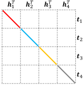
(a) DistMult.

(b) SimplE.

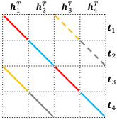
(c) ComplEx.

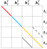
(d) Analogy.

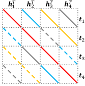
(e) QuatE.

Figure 1: The forms of $\bm{R}_{(\bm{r})}$ for representative BLMs (best viewed in color). Different colors correspond to different parts of $[\bm{r}_{1},\bm{r}_{2},\bm{r}_{3},\bm{r}_{4}]$ (red for $\bm{r}_{1}$, blue for $\bm{r}_{2}$, yellow for $\bm{r}_{3}$, gray for $\bm{r}_{4}$). Solid lines mean positive values, while dashed lines mean negative values. The empty parts have value zero.

3 Automated Bilinear Model

In the last decade, KG learning has been improving with new scoring function designs. However, as different KGs may have different properties, it is unclear how a proper scoring function can be designed for a particular KG. This raises the question: Can we automatically design a scoring function for a given KG? To address this question, we first provide a unified view of BLMs, and then formulate the design of scoring function as an AutoML problem: AutoBLM (“automated bilinear model”).

3.1 A Unified View of BLM

Recall from Section 2.1 that a BLM may operate in the real/complex/hypercomplex space. To write the different BLMs in the same form, we first unify them to the same representation space. The idea is to partition each of the embeddings $\bm{h},\bm{r},\bm{t}$ to $K=4$ equal-sized chunks, as $\bm{h}=[\bm{h}_{1},\dots,\bm{h}_{4}],\bm{r}=[\bm{r}_{1},\dots,\bm{r}_{4}]$ and $\bm{t}=[\bm{t}_{1},\dots,\bm{t}_{4}]$. The BLM is then written in terms of $\{\langle\bm{h}_{i},\bm{r}_{j},\bm{t}_{k}\rangle\}_{i,j,k\in\{1,\dots,4\}}$.

• DistMult [7], which uses $f(h,r,t)=\left\langle\bm{h},\bm{r},\bm{t}\right\rangle$. We simply split $\bm{h}\in\mathbb{R}^{d}$ (and analogously $\bm{r}$ and $\bm{t}$) into 4 parts as $\{\bm{h}_{1},\bm{h}_{2},\bm{h}_{3},\bm{h}_{4}\}$, where $\bm{h}_{i}\in\mathbb{R}^{d/4}$ for $i=1,2,3,4$. Obviously,

  $$\left\langle\bm{h},\bm{r},\bm{t}\right\rangle$$

  $$=\left\langle\bm{h}_{1},\bm{r}_{1},\bm{t}_{1}\right\rangle+\left\langle\bm{h}_{2},\bm{r}_{2},\bm{t}_{2}\right\rangle+\left\langle\bm{h}_{3},\bm{r}_{3},\bm{t}_{3}\right\rangle+\left\langle\bm{h}_{4},\bm{r}_{4},\bm{t}_{4}\right\rangle.$$

• SimplE [17] / CP [18], which uses $f(h,r,t)=\langle\hat{\bm{h}},\hat{\bm{r}},\underline{\bm{t}}\rangle+\langle\underline{\bm{t}},\underline{\bm{r}},\hat{\bm{h}}\rangle$. We split $\hat{\bm{h}}\in\mathbb{R}^{d}$ (and analogously $\hat{\bm{r}}$ and $\hat{\bm{t}}$) into 2 parts as $\{\bm{h}_{1},\bm{h}_{2}\}$ (where $\bm{h}_{1},\bm{h}_{2}\in\mathbb{R}^{d/2}$), and similarly $\underline{\bm{h}}$ as $\{\bm{h}_{3},\bm{h}_{4}\}$ (and analogously $\underline{\bm{r}}$ and $\underline{\bm{t}}$). Then,

  $$\langle\hat{\bm{h}},\hat{\bm{r}},\underline{\bm{t}}\rangle+\langle\underline{\bm{t}},\underline{\bm{r}},\hat{\bm{h}}\rangle$$

  $$=\left\langle\bm{h}_{1},\bm{r}_{1},\bm{t}_{3}\right\rangle+\left\langle\bm{h}_{2},\bm{r}_{2},\bm{t}_{4}\right\rangle+\left\langle\bm{h}_{3},\bm{r}_{3},\bm{t}_{1}\right\rangle+\left\langle\bm{h}_{4},\bm{r}_{4},\bm{t}_{2}\right\rangle.$$

• ComplEx [14] / HolE [15], which uses $f(h,r,t)=\text{Re}(\bm{h}\otimes\bm{r}\otimes\bar{\bm{t}})$, where $\bm{h},\bm{r},\bar{\bm{t}}$ are complex-valued. Recall that any complex vector $\bm{v}\in\mathbb{C}^{d}$ is of the form $\bm{v}_{r}+i\bm{v}_{i}$, where $\bm{v}_{r}\in\mathbb{R}^{d}$ is the real part and $\bm{v}_{i}\in\mathbb{R}^{d}$ is the imaginary part. Thus,

  $$\text{Re}(\bm{h}\otimes\bm{r}\otimes\bar{\bm{t}}) = \langle\bm{h}_{r},\bm{r}_{r},\bm{t}_{r}\rangle+\langle\bm{h}_{i},\bm{r}_{r},\bm{t}_{i}\rangle$$ (2)

  $$+\langle\bm{h}_{r},\bm{r}_{i},\bm{t}_{i}\rangle-\langle\bm{h}_{i},\bm{r}_{i},\bm{t}_{r}\rangle.$$

  We split $\bm{h}_{r}\in\mathbb{R}^{d}$ (and analogously $\bm{r}_{r}$ and $\bm{t}_{r}$) into 2 parts $\{\bm{h}_{1},\bm{h}_{2}\}$ (where $\bm{h}_{1},\bm{h}_{2}\in\mathbb{R}^{d/2}$), and similarly $\bm{h}_{i}=\{\bm{h}_{3},\bm{h}_{4}\}$ (and analogously $\bm{r}_{i}$ and $\bm{t}_{i}$). Then,

  $$\text{Re}(\bm{h}\otimes\bm{r}\otimes\bar{\bm{t}})$$

  $$\!\!=\!\! \!\!\big{(}\!\langle\bm{h}_{1},\!\bm{r}_{1},\!\bm{t}_{1}\rangle\!+\!\langle\bm{h}_{2},\!\bm{r}_{2},\!\bm{t}_{2}\rangle\!\big{)}\!+\!\big{(}\!\langle\bm{h}_{3},\!\bm{r}_{1},\!\bm{t}_{3}\rangle\!+\!\langle\bm{h}_{4},\!\bm{r}_{2},\!\bm{t}_{4}\rangle\!\big{)}$$

  $$\!\!+\big{(}\!\langle\bm{h}_{1},\!\bm{r}_{3},\!\bm{t}_{3}\rangle\!+\!\langle\bm{h}_{2},\!\bm{r}_{4},\!\bm{t}_{4}\rangle\!\big{)}\!-\!\big{(}\!\langle\bm{h}_{3},\!\bm{r}_{3},\!\bm{t}_{1}\rangle\!-\!\langle\bm{h}_{4},\!\bm{r}_{4},\!\bm{t}_{2}\rangle\!\big{)}.$$

• Analogy [16], which uses $f(h,r,t)=\langle\hat{\bm{h}},\hat{\bm{r}},\hat{\bm{t}}\rangle+\text{Re}\big{(}\underline{\bm{h}}\otimes\underline{\bm{r}}\otimes\bar{\underline{\bm{t}}}\big{)}$. We split $\hat{\bm{h}}\in\mathbb{R}^{d}$ (and analogously $\hat{\bm{r}}$ and $\hat{\bm{t}}$) into 2 parts $\{\bm{h}_{1},\bm{h}_{2}\}$ (where $\bm{h}_{1},\bm{h}_{2}\in\mathbb{R}^{d/2}$), and similarly $\underline{\bm{h}}\in\mathbb{C}^{d/2}$ (and analogously $\underline{\bm{r}}$ and $\underline{\bm{t}}$) into 2 parts $\{\bm{h}_{3},\bm{h}_{4}\}$ (where $\bm{h}_{3},\bm{h}_{4}\in\mathbb{R}^{d/2}$). Then,

  $$\langle\hat{\bm{h}},\hat{\bm{r}},\hat{\bm{t}}\rangle+\text{Re}\big{(}\underline{\bm{h}}\otimes\underline{\bm{r}}\otimes\bar{\underline{\bm{t}}}\big{)}$$

  $$=\left\langle\bm{h}_{1},\bm{r}_{1},\bm{t}_{1}\right\rangle+\left\langle\bm{h}_{2},\bm{r}_{2},\bm{t}_{2}\right\rangle+\left\langle\bm{h}_{3},\bm{r}_{3},\bm{t}_{3}\right\rangle+\left\langle\bm{h}_{3},\bm{r}_{4},\bm{t}_{4}\right\rangle$$

  $$\quad+\left\langle\bm{h}_{4},\bm{r}_{3},\bm{t}_{4}\right\rangle-\left\langle\bm{h}_{4},\bm{r}_{4},\bm{t}_{3}\right\rangle.$$

• QuatE [19], which uses $f(h,r,t)=\bm{h}\odot\bm{r}\odot\bm{t}$. Recall that any hypercomplex vector $\bm{v}\in\mathbb{H}^{d}$ is of the form $\bm{v}_{1}+i\bm{v}_{2}+j\bm{v}_{3}+k\bm{v}_{4}$, where $\bm{v}_{1},\bm{v}_{2},\bm{v}_{3},\bm{v}_{4}\in\mathbb{R}^{d}$. Thus,

  $$\bm{h}\odot\bm{r}\odot\bm{t}$$

  $$=\left\langle\bm{h}_{1},\bm{r}_{1},\bm{t}_{1}\right\rangle-\left\langle\bm{h}_{1},\bm{r}_{2},\bm{t}_{2}\right\rangle-\left\langle\bm{h}_{1},\bm{r}_{3},\bm{t}_{3}\right\rangle-\left\langle\bm{h}_{1},\bm{r}_{4},\bm{t}_{4}\right\rangle$$

  $$+\left\langle\bm{h}_{2},\bm{r}_{2},\bm{t}_{1}\right\rangle+\left\langle\bm{h}_{2},\bm{r}_{1},\bm{t}_{2}\right\rangle+\left\langle\bm{h}_{2},\bm{r}_{4},\bm{t}_{3}\right\rangle-\left\langle\bm{h}_{2},\bm{r}_{3},\bm{t}_{4}\right\rangle$$

  $$+\left\langle\bm{h}_{3},\bm{r}_{3},\bm{t}_{1}\right\rangle-\left\langle\bm{h}_{3},\bm{r}_{4},\bm{t}_{2}\right\rangle+\left\langle\bm{h}_{3},\bm{r}_{1},\bm{t}_{3}\right\rangle+\left\langle\bm{h}_{3},\bm{r}_{2},\bm{t}_{4}\right\rangle$$

  $$+\left\langle\bm{h}_{4},\bm{r}_{4},\bm{t}_{1}\right\rangle+\left\langle\bm{h}_{4},\bm{r}_{3},\bm{t}_{2}\right\rangle-\left\langle\bm{h}_{4},\bm{r}_{2},\bm{t}_{3}\right\rangle+\left\langle\bm{h}_{4},\bm{r}_{1},\bm{t}_{4}\right\rangle.$$

As $\langle\bm{h}_{i},\bm{r}_{k},\bm{t}_{j}\rangle=\bm{h}_{i}^{\top}\text{diag}\!\left(\bm{r}_{k}\right)\bm{t}_{j}$, all the above BLMs can be written in the form of a bilinear function

$$\bm{h}^{\top}\bm{R}_{(\bm{r})}\bm{t},$$ (3)

where $\bm{h}=[\bm{h}_{1}^{\top},\dots,\bm{h}_{4}^{\top}]^{\top},\bm{t}=[\bm{t}_{1};\dots;\bm{t}_{4}]\in\mathbb{R}^{d}$, and $\bm{R}_{(\bm{r})}\in\mathbb{R}^{d\times d}$ is a matrix with $4\times 4$ blocks, each block being either $\bm{0},\pm\text{diag}\!\left(\bm{r}_{1}\right),\dots$, or $\pm\text{diag}\!\left(\bm{r}_{4}\right)$. Figure 1 shows graphically the $\bm{R}_{(\bm{r})}$ for the BLMs considered.

3.2 Unified Bilinear Model

Using the above unified representation, the design of BLM becomes designing $\bm{R}_{(\bm{r})}$ in (3).

Definition 3 (Unified BiLinear Model).

The desired scoring function is of the form

$$f_{\bm{A}}({h},{r},{t})=\sum\nolimits_{i,j=1}^{K}\!{\emph{sign}}(A_{ij})\!\left\langle\bm{h}_{i},\bm{r}_{|A_{ij}|},\bm{t}_{j}\right\rangle,$$ (4)

where

$$\bm{A}\in\{0,\pm 1,\dots,\pm K\}^{K\times K}$$ (5)

is called the structure matrix. Here, we define $\bm{r}_{0}\equiv\bm{0}$, and $\emph{sign}(0)=0$.

It can be easily seen that this covers all the BLMs in Section 3.1 when $K=4$. Let $g_{K}(\bm{A},\bm{r})$ be a matrix with $K\times K$ blocks, with its $(i,j)$-th block:

$$[g_{K}(\bm{A},\bm{r})]_{ij}=\text{sign}(A_{ij})\cdot\text{diag}(\bm{r}_{|A_{ij}|}).$$ (6)

The form in (4) can be written more compactly as

$$f_{\bm{A}}({h},{r},{t})=\bm{h}^{\top}g_{K}(\bm{A},\bm{r})\bm{t}.$$ (7)

A graphical illustration is shown in Figure 2.

Figure 2: A graphical illustration of the proposed form of $f_{\bm{A}}({h},{r},{t})$.

The following Proposition gives a necessary and sufficient condition for the BLM with scoring function in (7) to be fully expressive. The proof is in Appendix A.1.

Proposition 1.

Let

$$\mathcal{C}\equiv\{\bm{r} \in\mathbb{R}^{K}\,|\,\bm{r}\neq\bm{0},$$

$$r[i]\in\{0,\pm 1,\dots,\pm K\},i=1,\dots,K\}.$$ (8)

Given an $\bm{A}$ in (5), the bilinear model with scoring function (7) is fully expressive if

1. $\exists\hat{\bm{r}}\in\mathcal{C}$ such that $g_{K}(\bm{A},\hat{\bm{r}})$ is symmetric (i.e., $g_{K}(\bm{A},\hat{\bm{r}})^{\top}=g_{K}(\bm{A},\hat{\bm{r}})$), and

2. $\exists\breve{\bm{r}}\in\mathcal{C}$ such that $g_{K}(\bm{A},\breve{\bm{r}})$ is skew-symmtric (i.e., $g_{K}(\bm{A},\breve{\bm{r}})^{\top}=-g_{K}(\bm{A},\breve{\bm{r}})$).

Table IV shows examples of $\hat{\bm{r}}$ and $\breve{\bm{r}}$ for the existing BLMs (ComplEx, HolE, Analogy, SimplE, CP, and QuatE), thus justifying that they are fully expressive.

TABLE IV: Example $\hat{\bm{r}}$ (resp. $\breve{\bm{r}}$) for the two conditions in Proposition 1.

model	$\hat{\bm{r}}$	$\breve{\bm{r}}$
ComplEx / HolE	$[1,2,0,0]$	$[0,0,3,4]$
Analogy	$[1,2,3,0]$	$[0,0,0,4]$
SimplE / CP	$[1,2,1,2]$	$[1,2,-1,-2]$
QuatE	$[1,0,0,0]$	$[0,2,3,4]$

3.3 Searching for BLMs

Using the family of unified BLMs in Definition 3 as the search space $\mathcal{A}$ for structure matrix $\bm{A}$, the search for a good data-specific BLM can be formulated as the following AutoML problem.

Definition 4 (Bilinear Model Search (AutoBLM)).

Let $F(\bm{P};\bm{A})$ be a KG embedding model (where $\bm{P}$ includes the entity embedding matrix $\bm{E}$ and relation embedding matrix $\bm{R}$, and $\bm{A}$ is the structure matrix) and $M(F,\mathcal{S})$ be the performance measurement of $F$ on triples $\mathcal{S}$ (the higher the better). The AutoBLM problem is formulated as:

$$\bm{A}^{*} \in\emph{Arg}\max\nolimits_{\bm{A}\in\mathcal{A}}M\left(F(\bm{P}^{*};\bm{A}),\mathcal{S}_{\text{val}}\right)$$ (9)

s.t. $$\bm{P}^{*} =\arg\max\nolimits_{\bm{P}}M\left(F(\bm{P};\bm{A}),\mathcal{S}_{\text{tra}}\right),$$ (10)

where

$$\mathcal{A}=\{\bm{A} =[A_{ij}]\in\mathbb{R}^{K\times K}$$

$$|\;A_{ij}\in\{0,\pm 1,\dots,\pm K\}\;\forall i,j=1,\dots,K\},$$ (11)

contains all the possible choices of $\bm{A}$, $\mathcal{S}_{\text{tra}}$ is the training set, and $\mathcal{S}_{\text{val}}$ is the validation set.

As a bi-level optimization problem, we first train the model to obtain $\bm{P}^{*}$ (converged model parameters) on the training set $\mathcal{S}_{\text{tra}}$ by (10), and then search for a better $\bm{A}$ (and consequently a better relation matrix $g_{K}(\bm{A},\bm{r})$) based on its performance $M$ on the validation set $\mathcal{S}_{\text{val}}$ in (9). Note that the objectives in (9) and (10) are non-convex, and the search space is large (with $(2K+1)^{K^{2}}$ candidates, as can be seen from (5)). Thus, solving (10) can be expensive and challenging.

3.4 Degenerate and Equivalent Structures

In this section, we introduce properties specific to the proposed search space $\mathcal{A}$. A careful exploitation of these would be key to an efficient search.

3.4.1 Degenerate Structures

Obviously, not all structure matrices in (5) are equally good. For example, if all the nonzero blocks in $g_{K}(\bm{A},\bm{r})$ are in the first column, $f_{\bm{A}}$ will be zero for all head embeddings with $\bm{h}_{1}=\bm{0}$. These structures should be avoided.

Definition 5 (Degenerate structure).

Matrix ${\bm{A}}$ is degenerate if (i) there exists $\bm{h}\neq{\bf 0}$ such that $\bm{h}^{\top}g_{K}(\bm{A},\bm{r})\bm{t}=0,\forall\bm{r},\bm{t}$; or (ii) there exists $\bm{r}\neq{\bf 0}$ such that $\bm{h}^{\top}g_{K}(\bm{A},\bm{r})\bm{t}=0,\forall\bm{h},\bm{t}$.

With a degenerate ${\bm{A}}$, the triple $(h,r,t)$ is always non-plausible for every nonzero head embedding $\bm{h}$ or relation embedding $\bm{r}$, which limits expressiveness of the scoring function. The following Proposition shows that it is easy to check whether $\bm{A}$ is degenerate. Its proof is in Appendix A.2.

Proposition 2.

$\bm{A}$ is not degenerate if and only if $\emph{rank}(\bm{A})=K$ and $\{1,\dots,K\}\subset\{|A_{ij}|:i,j=1,\dots,K\}$.

Since $K$ is very small (which is equal to 4 here), the above conditions are inexpensive to check. Hence, we can efficiently filter out degenerate $\bm{A}$’s and avoid wasting time in training and evaluating these structures.

3.4.2 Equivalence

In general, two different $\bm{A}$’s can have the same performance (as measured by $F$ in Definition 4). This is captured in the following notion of equivalence. If a group of $\bm{A}$’s are equivalent, we only need to evaluate one of them.

Definition 6 (Equivalence).

Let ${\bm{P}}^{*}=\arg\max\nolimits_{\bm{P}}$ $M(F(\bm{P};\bm{A}),\mathcal{S})$ and ${\bm{P}^{\prime}}^{*}=\arg\max\nolimits_{\bm{P}^{\prime}}$ $M(F(\bm{P^{\prime}};\bm{A}^{\prime}),\mathcal{S})$. If $\bm{A}\neq\bm{A}^{\prime}$ but $M\big{(}F({\bm{P}}^{*};\bm{A}),\mathcal{S}\big{)}$ $=M\big{(}F({\bm{P}^{\prime}}^{*};\bm{A}^{\prime}),\mathcal{S}\big{)}$ for all $\mathcal{S}$, then $\bm{A}$ is equivalent to $\bm{A}^{\prime}$ (denoted $\bm{A}\equiv\bm{A}^{\prime}$).

The following Proposition shows several conditions for two structures to be equivalent. Its proof is in Appendix A.3. Examples are shown in Figure 3.

(a) Analogy.

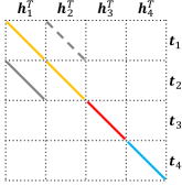
(b) Permuting rows and columns.

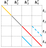
(c) Permuting values.

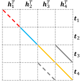
(d) Flipping signs.

Figure 3: Illustration of $\bm{R}_{(\bm{r})}$ for Analogy (Figure 3(a)) and three example equivalent structures based on the conditions in Proposition 3. Figure 3(b) permutes the index $[1,2,3,4]$ of rows and columns in $\bm{A}$ to $[3,4,1,2]$; Figure 3(c) permutes the values $[1,2,3,4]$ in $\bm{A}$ to $[3,4,1,2]$; Figure 3(d) flips the signs of values $[1,2,3,4]$ in $\bm{A}$ to $[-1,2,-3,4]$.

Proposition 3.

Given an $\bm{A}$ in (5), construct $\bm{\Phi}_{\bm{A}}\in\mathbb{R}^{K\times K^{2}}$ such that $[\bm{\Phi}_{\bm{A}}]_{|A_{ij}|,(i-1)K+j}=\emph{sign}(A_{ij})$ if $|A_{ij}|\in\{1,\dots,K\}$, and 0 otherwise. Two structure matrices $\bm{A}$ and $\bm{A}^{\prime}$ are equivalent if any one of the following conditions is satisfied.

1. Permuting rows and columns: There exists a permutation matrix $\bm{\Pi}\in\mathbb{\{}0,1\}^{K\times K}$ such that $\bm{A}^{\prime}=\bm{\Pi}^{\top}\bm{A}\bm{\Pi}$.

2. Permuting values: There exists a permutation matrix $\bm{\Pi}\in\{0,1\}^{K\times K}$ such that $\bm{\Phi}_{\bm{A}^{\prime}}=\bm{\Pi}\bm{\Phi}_{\bm{A}}$;

3. Flipping signs: There exists a sign vector $\bm{s}\in\{\pm 1\}^{K}$ such that $[\bm{\Phi}_{\bm{A}^{\prime}}]_{i,\cdot}=s_{i}\cdot[\bm{\Phi}_{\bm{A}}]_{i,\cdot},\forall i=1,\dots,K$.

There are $K!$ possible permutation matrices for conditions (i) and (ii), and $2^{K}$ possible sign vectors for condition (iii). Hence, one has to check a total of $(K!)^{2}2^{K}$ combinations.

4 Search Algorithm

In this section, we design efficient algorithms to search for the structure matrix $\bm{A}$ in (5). As discussed in Section 2.3.1, the model-based approach requires a proper surrogate model for such a complex space. Thus, we will focus on the sample-based approach, particularly on the progressive algorithm and evolutionary algorithm. To search efficiently, one needs to (i) ensure that each new $\bm{A}$ is neither degenerate nor equivalent to an already-explored structure; and (ii) the scoring function $f_{\bm{A}}({h},{r},{t})$ obtained from the new $\bm{A}$ is likely to have high performance. These can be achieved by designing an efficient filter (Section 4.1) and performance predictor (Section 4.2). Then, we introduce two search algorithms: progressive search (Section 4.3) and evolutionary algorithm (Section 4.4).

4.1 Filtering Degenerate and Equivalent Structures

Algorithm 1 shows the filtering procedure. First, step 2 removes degenerate structure matrices by using the conditions in Proposition 2. Step 3 then generates a set of $(K!)^{2}2^{K}$ structures that are equivalent to $\bm{A}$ (Proposition 3). $\bm{A}$ is filtered out if any of its equivalent structures appears in the set $\mathcal{H}$ containing structure matrices that have already been explored. As $K$ is small, this filtering cost is very low compared with the cost of model training in (10).

Algorithm 1 Filtering degenerate and equivalent structure matrices. The output is “False” if the input structure matrix $\bm{A}$ is to be filtered out.

0:  $\bm{A}$: a $K\times K$ structure matrix, $\mathcal{H}$: a set of structures.

1:  initialization: $\mathcal{Q}(\bm{A},\mathcal{H})=\text{True}$.

2:  if $\det(\bm{A})=0$ or $\{1,\dots,K\}\not\subset\{|A_{ij}|:i,j=1,\dots,K\}$, then $\mathcal{Q}(\bm{A},\mathcal{H})=\text{False}$.

3:  generate a set of equivalent structures $\{\bm{A}^{\prime}\!:\!\bm{A}^{\prime}\!\equiv\!\bm{A}\}$ by enumerating permutation matrices $\bm{P}$’s and sign vectors $\bm{s}$’s.

4:  for $\bm{A}^{\prime}$ in $\{\bm{A}^{\prime}:\bm{A}^{\prime}\equiv\bm{A}\}$ do

5:     if $\bm{A}^{\prime}\in\mathcal{H}$, then $\mathcal{Q}(\bm{A},\mathcal{H})=\text{False}$, and exit the loop.

6:  end for

7:  return  $\mathcal{Q}(\bm{A},\mathcal{H})$.

4.2 Performance Predictor

After collecting $N$ structures in $\mathcal{H}$, we construct a predictor $\mathcal{P}$ to estimate the goodness of each $\bm{A}$. As mentioned in Section 2.3, search efficiency depends heavily on how to evaluate the candidate models.

A highly efficient approach is parameter sharing, as is popularly used in one-shot neural architecture search (NAS) [47, 31]. However, parameter sharing can be problematic when used to predict the performance of scoring functions. Consider the following two $\bm{A}$’s: (i) $\bm{A}_{1}$ is a $4\times 4$ matrix of all $+1$’s, and so $f_{\bm{A}_{1}}(h,r,t)=\sum_{i,j=1}^{4}\langle\bm{h}_{i},\bm{r}_{1},\bm{t}_{j}\rangle$, and (ii) $\bm{A}_{2}$ is a $4\times 4$ matrix of all $-1$’s, and so $f_{\bm{A}_{2}}(h,r,t)=-\sum_{i,j=1}^{4}\langle\bm{h}_{i},\bm{r}_{1},\bm{t}_{j}\rangle=-f_{\bm{A}_{1}}(h,r,t)$. When parameter sharing is used, it is likely that the performance predictor will output different scores for $\bm{A}_{1}$ and $\bm{A}_{2}$. However, from Proposition 3, by setting $\bm{s}=[-1,-1,-1,-1]$ in condition (iii), we have $\bm{A}_{1}\equiv\bm{A}_{2}$ and thus they indeed have the same performance. This problem will also be empirically demonstrated in Section 5.1.8. Hence, instead, we train and evaluate the models separately as in the stand-alone NAS evaluation [30, 49].

Algorithm 2 Construction of the symmetry-related feature (SRF) vectors.

0:  structure matrix $\bm{A}$.

1:  initialization: $\bm{\alpha},\bm{\beta}:=\bm{0}$.

2:  for $\bm{r}\in\mathcal{C}$ do

3:     if $\bm{r}\neq\bm{0}$ then

4:        $x=\big{|}\{i:r_{i}\!=\!0\}\big{|}$;

5:        $y=\big{|}\{j>0:r_{i}\!=\!j\text{ or }r_{i}\!=\!-j\}\big{|}$; // for symmetric case

6:        if $g_{K}(\bm{A},\bm{r})\!-\!g_{K}(\bm{A},\bm{r})^{\top}\!\!=\!\mathbf{0}$ then $\alpha_{(x,y)}\!=\!1$; // for skew-symmetric case

7:        if $g_{K}(\bm{A},\bm{r})\!+\!g_{K}(\bm{A},\bm{r})^{\top}\!\!=\!\mathbf{0}$ then $\beta_{(x,y)}\!=\!1$;

8:     end if

9:  end for

10:  return  $[\text{vec}(\bm{\alpha});\text{vec}(\bm{\beta})]$.

Recall from Section 2.1 that it is desirable for the scoring function to be fully expressive. Proposition 1 shows that this requires looking for a $\hat{\bm{r}}\in\mathcal{C}$ such that $g_{K}(\bm{A},\hat{\bm{r}})$ is symmetric and a $\breve{\bm{r}}\in\mathcal{C}$ such that $g_{K}(\bm{A},\breve{\bm{r}})$ is skew-symmetric. This motivates us to examine each of the $(2K+1)^{K}-1$ ${\bm{r}}$’s in $\mathcal{C}$ (defined in (8)) and see whether it leads to a symmetric or skew-symmetric $g_{K}(\bm{A},{\bm{r}})$. However, directly using all these $(2K+1)^{K}-1$ choices as features to a performance predictor can be computationally expensive. Instead, empirically we find that the following two features can be used to group the scoring functions: (i) number of zeros in $\bm{r}$: $|\{i\in\{1,\dots,K\}:r_{i}=0\}|$; and (ii) number of nonzero absolute values in $\bm{r}$: $|\{j>0:r_{i}=j\text{ or }r_{i}=-j,\;i\in\{1,\dots,K\}\}|$. The possible choices is reduced to $K(K+1)/2$ (groups of scoring functions). We keep two symmetry-related feature (SRF) as $\bm{\alpha}$ and $\bm{\beta}$. If $g_{K}(\bm{A},\bm{r})$ is symmetric (resp. skew-symmetric) for any ${\bm{r}}$ in $\mathcal{C}$, the entry in $\bm{\alpha}$ (resp. $\bm{\beta}$) corresponding to ${\bm{r}}$ is set to 1. The construction process is also shown in Algorithm 2. Finally, the SRF vector is composed with $\text{vec}(\bm{\alpha})$ and $\text{vec}(\bm{\beta})$, which vectorize the values in $\bm{\alpha}$ and $\bm{\beta}$, and fed as input to a two-layer MLP for performance prediction.

Algorithm 3 Progressive search algorithm (AutoBLM).

0:  $I$: number of top structures; $N$: number of generated structures; $P$: number of structures selected by $\mathcal{P}$; $b_{0}$: number of nonzero elements in initial structures; filter $\mathcal{Q}$ and performance predictor $\mathcal{P}$.

1:  initialization: $b:=b_{0}$, create a candidate set $\mathcal{H}^{b}=\emptyset$;

2:  for each $\bm{A}^{(b)}\in\{\bm{A}^{(b)}\}$ do

3:     if $\mathcal{Q}(\bm{A}^{(b)},\mathcal{H}^{b})$ from Algorithm 1 is true then $\mathcal{H}^{b}\leftarrow\mathcal{H}^{b}\cup\{\bm{A}^{(b)}\}$;

4:     if $|\mathcal{H}^{b}|=I$, break loop;

5:  end for

6:  train and evaluate all $\bm{A}^{(b)}$’s in $\mathcal{H}^{b}$;

7:  add $\bm{A}^{(b)}$’s to $\mathcal{T}^{b}$ and record the performance in $\mathcal{Y}^{b}$;

8:  update predictor $\mathcal{P}$ with records in $(\mathcal{T}^{b},\mathcal{Y}^{b})$.

9:  repeat

10:     $b:=b+1$;

11:     $\mathcal{H}^{b}=\emptyset$;

12:     repeat

13:        randomly select a top-$I$ structure ${\bm{A}^{b-1}}\in\mathcal{T}^{b-1}$;

14:        randomly generate $i_{b},j_{b},k_{b}\in\{1,\dots,K\}$, $s_{b}\in\{\pm 1\}$, and form $\bm{A}^{(b)}$ with $f_{\bm{A}^{(b)}}\leftarrow f_{\bm{A}^{b-1}}+s_{b}\left\langle\bm{h}_{i_{b}},\bm{r}_{k_{b}},\bm{t}_{j_{b}}\right\rangle$;

15:        if $\mathcal{Q}(\bm{A}^{(b)},\mathcal{H}^{b}\cup\mathcal{T}^{b})$ from Algorithm 1 is true then $\mathcal{H}^{b}\leftarrow\mathcal{H}^{b}\cup\{\bm{A}^{(b)}\}$;

16:     until $\left|\mathcal{H}^{b}\right|=N$

17:     select top-$P$ $\bm{A}^{(b)}$’s in $\mathcal{H}^{b}$ based on the predictor $\mathcal{P}$;

18:     train embeddings and evaluate the performance of $\!\bm{A}^{(b)}$’s;

19:     add $\bm{A}^{(b)}$’s in $\mathcal{T}^{b}$ and record the performance in $\mathcal{Y}^{b}$;

20:     update the predictor (the following commented out) $\mathcal{P}$ with ($\mathcal{T}={\mathcal{T}}^{b_{0}}\cup\dots\cup{\mathcal{T}}^{b}$, ${\mathcal{Y}}={\mathcal{Y}}^{b_{0}}\cup\dots\cup{\mathcal{Y}}^{b}$);

21:  until budget is exhausted or $b=K^{2}$;

22:  select the top-$I$ structures in $\mathcal{T}$ based on performance in $\mathcal{Y}$ to form the set $\mathcal{I}$.

23:  return  $\mathcal{I}$.

4.3 Progressive Algorithm

To explore the search space $\mathcal{A}$ in (11), the simplest approach is by direct sampling. However, it can be expensive as the space is large. Note from (4) that the complexity of $f_{\bm{A}}({h},{r},{t})$ is controlled by the number of nonzero elements in $\bm{A}$. Inspired by [49], we propose in this section a progressive algorithm that starts with $\bm{A}$’s having only a few nonzero elements, and then gradually expands the search space by allowing more nonzeros.

The procedure, which is called AutoBLM, is in Algorithm 3. Let $\bm{A}^{(b)}$ be an $\bm{A}$ with $b$ nonzero elements, and the corresponding BLM be $f_{\bm{A}^{(b)}}$. In step 1, we initialize $b$ to some $b_{0}$ and create an empty candidate set $\mathcal{H}^{b}$. As $\bm{A}$’s with fewer than $K$ nonzero elements are degenerate (Proposition 2), we use $b_{0}=K$. We first sample positions of $b_{0}$ nonzero elements, and then randomly assign them values in $\{\pm 1,\pm 2,\dots,\pm K\}$. The other entries are set to zero.

Steps 2-5 filter away degenerate and equivalent structures. The number of nonzero elements $b$ is then increased by $1$ (step 10). For each such $b$, steps 12-16 greedily select a top-performing structure (evaluated based on the mean reciprocal rank (MRR) [3] performance on $\mathcal{S}_{\text{val}}$) in $\mathcal{T}^{b-1}$, and generate $N$ candidates. All the candidates are checked by the filter $\mathcal{Q}$ (Section 4.1) to avoid degenerate or equivalent solutions. Next, the predictor $\mathcal{P}$ in Section 4.2 selects the top-$P$ $\bm{A}^{(b)}$’s, which are then trained and evaluated in step 18. The training data for $\mathcal{P}$ is collected with the recorded structures and performance in $(\mathcal{T},\mathcal{Y})$ at step 20. Finally, the top-$I$ structures in $\mathcal{T}$ evaluated by the corresponding performance in $\mathcal{Y}$ are returned.

Algorithm 4 Evolutionary search algorithm. (AutoBLM+).

0:  $I$: number of top structures; $N$: number of generated structures; $P$: number of structures selected by $\mathcal{P}$; $b_{0}$: number of nonzero elements in initial structures; filter $\mathcal{Q}$, and performance predictor $\mathcal{P}$.

1:  initialization: $\mathcal{I}=\emptyset$;

2:  for each $\bm{A}\in\{\bm{A}^{(b_{0})}\}$ do

3:     if $\mathcal{Q}(\bm{A},\mathcal{I})$ from Algorithm 1 is true then $\mathcal{I}\leftarrow\mathcal{I}\cup\left\{\bm{A}\right\}$;

4:     if $|\mathcal{I}|=I$, break loop;

5:  end for

6:  train and evaluate all $\bm{A}$’s in $\mathcal{I}$;

7:  add $\bm{A}$’s to $\mathcal{T}$ and record the performance in $\mathcal{Y}$;

8:  repeat

9:     update predictor $\mathcal{P}$ with records in $(\mathcal{T},\mathcal{Y})$.

10:     repeat

11:        $\mathcal{H}=\emptyset$;

12:        mutation: sample $\bm{A}\in\mathcal{I}$ and mutate to $\bm{A}_{\text{new}}$; or

13:        crossover: sample $\bm{A}_{(a)},\bm{A}_{(b)}\!\in\!\mathcal{I}$, and use crossover to generate $\bm{A}_{\text{new}}$;

14:        if $\mathcal{Q}(\bm{A}_{\text{new}},\mathcal{H}\cup\mathcal{T})$ is true by Algorithm 1, then $\mathcal{H}\leftarrow\mathcal{H}\cup\left\{\bm{A}_{\text{new}}\right\}$;

15:     until $|\mathcal{H}|=N$;

16:     select top-$P$ structures $\bm{A}$ in $\mathcal{H}$ based on the the predictor $\mathcal{P}$;

17:     for  each top-$P$ structure $\bm{A}$  do

18:        train embeddings and evaluate the performance of ${\bm{A}}$;

19:        survive: update $\mathcal{I}$ with $\bm{A}$ if ${\bm{A}}$ is better than the worst structure in $\mathcal{I}$;

20:     end for

21:     add $\bm{A}$’s in $\mathcal{T}$ and record the performance in $\mathcal{Y}$;

22:  until budget is exhausted;

23:  return  $\mathcal{I}$.

4.4 Evolutionary Algorithm

While progressive search can be efficient, it may not fully explore the search space and can lead to sub-optimal solutions [51]. The progressive search can only generate structures from fewer non-zero elements to more ones. Thus, it can not visit and adjust the structures with fewer non-zero elements when $b$ is increased. To address these problems, we consider in this section the use of evolutionary algorithms [52].

The procedure, which is called AutoBLM+, is in Algorithm 4. As in Algorithm 3, we start with structures having $b_{0}=K$ nonzero elements. Steps 1-6 initializes a set $\mathcal{I}$ of $I$ non-degenerate and non-equivalent structures. The main difference with Algorithm 3 is in steps 8-15, in which new structures are generated by mutation and crossover. For a given structure $\bm{A}$, mutation changes the value of each entry to another one in $\{0,\pm 1,\dots,\pm K\}$ with a small probability $p_{m}$. For crossover, given two structures $\bm{A}_{(a)}$ and $\bm{A}_{(b)}$, each entry of the new structure has equal probabilities to be selected from the corresponding entries in $\bm{A}_{(a)}$ or $\bm{A}_{(b)}$. After mutation or crossover, we check if the newly generated $\bm{A}_{\text{new}}$ has to be filtered out. After $N$ structures are collected, we use the performance predictor $\mathcal{P}$ in Section 4.2 to select the top-$P$ structures. These are then trained and evaluated for actual performance. Finally, structures in $\mathcal{I}$ with performance worse than the newly evaluated ones are replaced (step 19).

5 Experiments

In this section, experiments are performed on a number of KG tasks. Algorithm 5 shows the general procedure for each task. First, we find a good hyper-parameter setting to train and evaluate different structures (steps 2-6). Based on the observation that the performance ranking of scoring functions is consistent across different $d$’s (details are in Appendix C), we set $d$ to a smaller value ($64$) to reduce model training time. The search algorithm is then used to obtain the set $\mathcal{I}$ of top-$I$ structures (step 8). Finally, the hyper-parameters are fine-tuned with a larger $d$, and the best structure selected (steps 10-14). Experiments are run on a RTX 2080Ti GPU with 11GB memory. All algorithms are implemented in python [53].

Algorithm 5 Experimental procedure for each KG task. Here, $H\!P$ denotes the hyper-parameters $\{\eta,\lambda,m,d\}$.

1:  // stage 1: configure hyper-parameters for scoring function search.

2:  for $i=1,\dots,10$ do

3:     fix $d=64$, randomly select $\eta_{i}$$\in$$[0$$,1]$, $\lambda_{i}$$\in$$[10^{-5}$$,10^{-1}]$ and $m_{i}\in\{256$$,512$$,1024\}$;

4:     train SimplE with $H\!P_{i}=\{\eta_{i},\lambda_{i},m_{i},d\}$, and evaluate the validation MRR;

5:  end for

6:  select the best hyper-parameter setting $\bar{H\!P}\in\{H\!P_{i}\}_{i=1}^{10}$;

7:  // stage 2: search scoring function

8:  using hyper-parameter setting $\bar{H\!P}$, obtain the set $\mathcal{I}$ of top-$I$ structures from Algorithm 3 or Algorithm 4;

9:  // stage 3: fine-tune the obtained scoring function

10:  for $j=1,\dots,50$ ($j=1,\dots,10$ for YAGO3-10) do

11:     randomly select a structure $\bm{A}_{j}\in\mathcal{I}$;

12:     randomly select $\eta_{j}\in[0,1]$, $\lambda_{j}\in[10^{-5},10^{-1}]$, $m_{j}\in\{256,512,1024\}$, and $d_{j}\in\{256,512,1024,2048\}$;

13:     train the KG learning model with structure $\bm{A}_{j}$ and hyper-parameter setting ${H\!P}_{j}=\{\eta_{j},\lambda_{j},m_{j},d_{j}\}$

14:  end for

15:  select the best structure $\{\bm{A}^{*},{H\!P}^{*}\}\in\{\bm{A}_{j},{H\!P}_{j}\}_{j=1}^{50}$.

5.1 Knowledge Graph (KG) Completion

In this section, we perform experiments on KG completion as introduced in Section 2.2.1. we use the full multi-class log-loss [18], which is more robust and has better performance than negative sampling [18, 33].

5.1.1 Setup

Datasets. Experiments are performed on the following popular benchmark datasets: WN18, FB15k, WN18RR, FB15k237, YAGO3-10, ogbl-biokg and ogbl-wikikg2 (Table V). WN18 and FB15k are introduced in [10]. WN18 is a subset of the lexical database WordNet [54], while FB15k is a subset of the Freebase KG [55] for human knowledge. WN18RR [21] and FB15k237 [56] are obtained by removing the near-duplicates and inverse-duplicate relations from WN18 and FB15k. YAGO3-10 is created by [21], and is a subset of the semantic KG YAGO [57], which unifies WordNet and Wikipedia. The ogbl-biokg and ogbl-wikikg2 datasets are from the open graph benchmark (OGB) [58], which contains realistic and large-scale datasets for graph learning. The ogbl-biokg dataset is a biological KG describing interactions among proteins, drugs, side effects and functions. The ogbl-wikikg2 dataset is extracted from the Wikidata knowledge base [59] describing relations among entities in Wikipedia.

TABLE V: Statistics of the KG completion datasets.

			number of samples
data set	#entity	#relation	training	validation	testing
WN18 [10]	40,943	18	141,442	5,000	5,000
FB15k [10]	14,951	1,345	484,142	50,000	59,071
WN18RR [21]	40,943	11	86,835	3,034	3,134
FB15k237 [56]	14,541	237	272,115	17,535	20,466
YAGO3-10 [60]	123,188	37	1,079,040	5,000	5,000
ogbl-biokg	94k	51	4,763k	163k	163k
ogbl-wikikg2	2500k	535	16,109k	429k	598k

TABLE VI: Testing performance of MRR, H@1 and H@10 on KG completion. The best model is highlighted in bold and the second best is underlined. “–” means that results are not reported in those papers or their code on that data/metric is not available. CompGCN uses the entire KG in each iteration and so runs out of memory on the larger data sets of WN18, FB15k and YAGO3-10.

		WN18			FB15k			WN18RR			FB15k237			YAGO3-10
model		MRR	H@1	H@10	MRR	H@1	H@10	MRR	H@1	H@10	MRR	H@1	H@10	MRR	H@1	H@10
(TDM)	TransH	0.521	—	94.5	0.452	—	76.6	0.186	—	45.1	0.233	—	40.1	—	—	—
	RotatE	0.949	94.4	95.9	0.797	74.6	88.4	0.476	42.8	57.1	0.338	24.1	53.3	0.488	39.6	66.3
	PairE	—	—	—	0.811	76.5	89.6	—	—	—	0.351	25.6	54.4	—	—	—
(NNM)	ConvE	0.942	93.5	95.5	0.745	67.0	87.3	0.46	39.	48.	0.316	23.9	49.1	0.52	45.	66.
	RSN	0.94	92.2	95.3	—	—	—	—	—	—	0.28	20.2	45.3	—	—	—
	Interstellar	—	—	—	—	—	—	0.48	44.0	54.8	0.32	23.3	50.8	0.51	42.4	66.4
	CompGCN	—	—	—	—	—	—	0.479	44.3	54.6	0.355	26.4	53.5	—	—	—
(BLM)	TuckER	0.953	94.9	95.8	0.795	74.1	89.2	0.470	44.3	52.6	0.358	26.6	54.4	—	—	—
	DistMult	0.821	71.7	95.2	0.775	71.4	87.2	0.443	40.4	50.7	0.352	25.9	54.6	0.552	47.1	68.9
	SimplE/CP	0.950	94.5	95.9	0.826	79.4	90.1	0.462	42.4	55.1	0.350	26.0	54.4	0.565	49.1	71.0
	HolE/ComplEx	0.951	94.5	95.7	0.831	79.6	90.5	0.471	43.0	55.1	0.345	25.3	54.1	0.563	49.0	70.7
	Analogy	0.950	94.6	95.7	0.816	78.0	89.8	0.467	42.9	55.4	0.348	25.6	54.7	0.557	48.5	70.4
	QuatE	0.950	94.5	95.9	0.782	71.1	90.0	0.488	43.8	58.2	0.348	24.8	55.0	0.556	47.4	70.4
AutoBLM		0.952	94.7	96.1	0.853	82.1	91.0	0.490	45.1	56.7	0.360	26.7	55.2	0.571	50.1	71.5
AutoBLM+		0.952	94.7	96.1	0.861	83.2	91.3	0.492	45.2	56.7	0.364	27.0	55.3	0.577	50.2	71.5

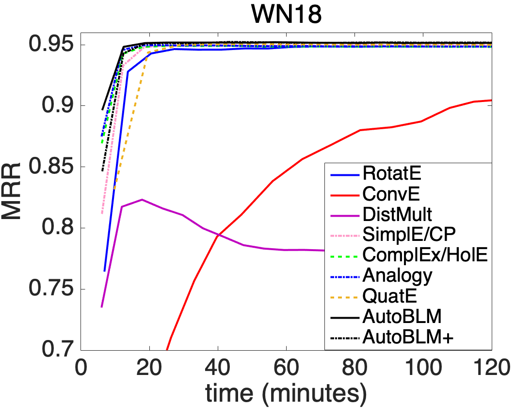
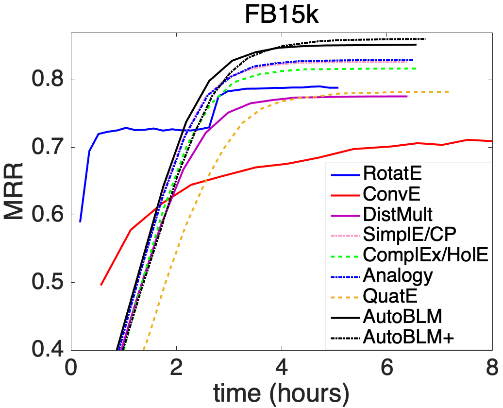
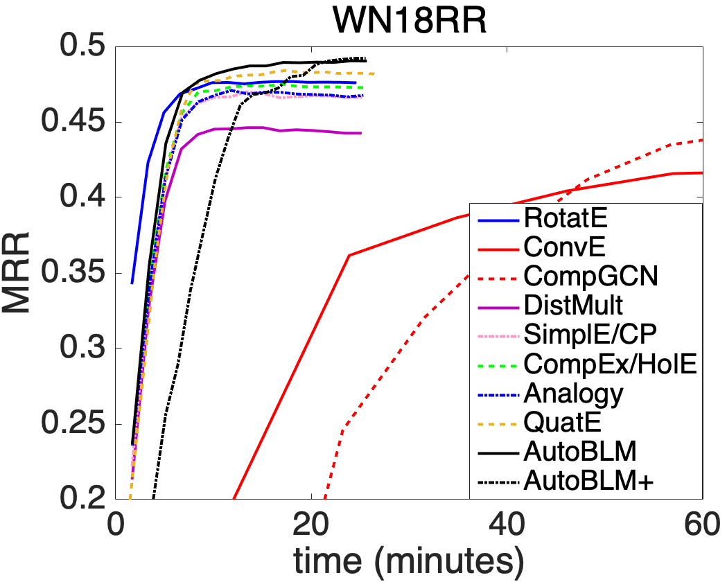
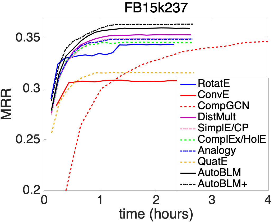
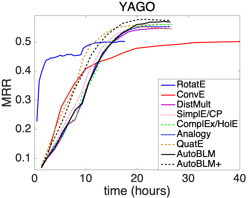
Figure 4: Convergence of the testing MRR versus running time on the KG completion task.

Baselines. For AutoBLM and AutoBLM+, we select the structure for evaluation from the set returned by Algorithm 3 or 4 based on the MRR performance on the validation set.

For WN18, FB15k, WN18RR, FB15k237, YAGO3-10, AutoBLM and AutoBLM+ are compared with the following popular human-designed KG embedding models: (i) TDM, including TransH [11], RotatE [13] and PairE [61]; (ii) NNM, including ConvE [21], RSN [22] and CompGCN [24]; (iii) BLM, including TuckER [35], Quat [19], DistMult [7], ComplEx [14], HolE [15], Analogy [16] SimplE [17], and CP [18]. We do not compare with NASE [62] as its code is not publicly available.

For ogbl-biokg and ogbl-wikikg2 [58], we compare with the models reported in the OGB leaderboard, namely, TransE [10], RotatE, PairE, DistMult, and ComplEx.

Performance Measures. The learned $f_{\bm{A}}(h,r,t)$ is evaluated in the context of link prediction. Following  [7, 14, 16, 17, 21, 3], for each triple $(h,r,t)$, we first take $(?,r,t)$ as the query and obtain the filtered rank on the head

$$\text{rank}_{h}=\left|\left\{e\in\mathcal{E}:\begin{matrix}\big{(}f(e,r,t)\geq f(h,r,t)\big{)}\wedge\\ \big{(}(e,r,t)\notin\mathcal{S}_{\text{tra}}\cup\mathcal{S}_{\text{val}}\cup\mathcal{S}_{\text{tst}}\big{)}\end{matrix}\right\}\right|+1,$$ (12)

where $\mathcal{S}_{\text{tra}},\mathcal{S}_{\text{val}},\mathcal{S}_{\text{tst}}$ are the training, validation, and test sets, respectively. Next we take $(h,r,?)$ as the query and obtain the filtered rank on the tail

$$\text{rank}_{t}\!=\!\left|\left\{e\in\mathcal{E}:\begin{matrix}\big{(}f(h,r,e)\geq f(h,r,t)\big{)}\wedge\\ \big{(}(h,r,e)\notin\mathcal{S}_{\text{tra}}\cup\mathcal{S}_{\text{val}}\cup\mathcal{S}_{\text{tst}}\big{)}\end{matrix}\right\}\right|\!+\!1.$$ (13)

The following metrics are computed from both the head and tail ranks on all triples: (i) Mean reciprocal ranking (MRR):

$$\text{MRR}=\frac{1}{2|\mathcal{S}|}\sum_{(h,r,t)\in\mathcal{S}}\!\!\Big{(}\frac{1}{\text{rank}_{h}}+\frac{1}{\text{rank}_{t}}\Big{)};$$

and (ii) H@$k$: ratio of ranks no larger than $k$, i.e.,

$$\text{H}@k=\frac{1}{2|\mathcal{S}|}\sum_{(h,r,t)\in\mathcal{S}}\!\!\Big{(}\mathbb{I}(\text{rank}_{h}\leq k)+\mathbb{I}(\text{rank}_{t}\leq k)\Big{)},$$

where $\mathbb{I}(a)=1$ if $a$ is true, otherwise $0$. The larger the MRR or H@$k$, the better is the embedding. Other metrics for the completion task [63, 64] can also be adopted here.

For ogbl-biokg and ogbl-wikikg2 [58], we only use the MRR as the H@$k$ is not reported by the baselines in the OGB leaderboard.

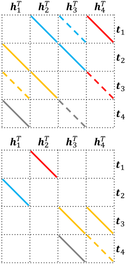
(a) WN18.

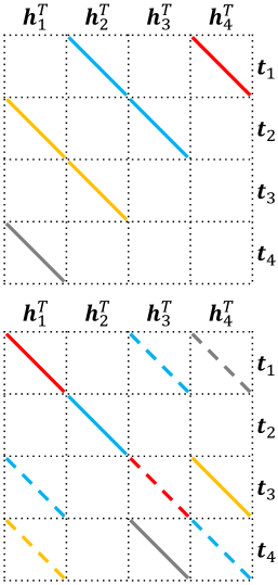
(b) FB15k.

(c) WN18RR.

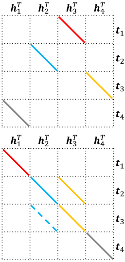
(d) FB15k237.

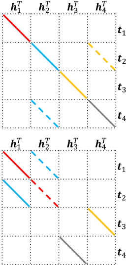
(e) YAGO3-10.

Figure 5: Graphical illustration of the BLMs obtained by AutoBLM (top) and AutoBLM+ (bottom) on the KG completion task (Section 5.1.2). Different colors correspond to different parts of $[\bm{r}_{1}$(red), $\bm{r}_{2}$(blue), $\bm{r}_{3}$(yellow), $\bm{r}_{4}$(gray)$]$. Solid lines mean positive values, while dashed lines mean negative values. The empty parts have value zero.

Hyper-parameters. The search algorithms have the following hyper-parameters: (i) $N$: number of candidates generated after filtering; (ii) $P$: number of scoring functions selected by the predictor; (iii) $I$: number of top structures selected in Algorithm 3 (step 13), or the number of structures survived in $\mathcal{I}$ in Algorithm 4; and (iv) $b_{0}$: number of nonzero elements in the initial set. Unless otherwise specified, we use $N=128$, $P=8$, $I=8$ and $b_{0}=K$. For the evolutionary algorithm, the mutation and crossover operations are selected with equal probabilities. When mutation is selected, the value of each entry has a mutation probability of $p_{m}=2/K^{2}$. A budget is used to terminate the algorithm. This is set to 256 structures on WN18, FB15k, WN18RR, FB15k-237, 128 on YAGO3-10, 64 on ogbl-biokg, and 32 on ogbl-wikikg2.

We follow [18, 14] to use Adagrad [65] as optimizer. The Adagrad hyper-parameters are selected from the following ranges: learning rate $\eta$ in $[0,1]$, $\ell_{2}$-penalty $\lambda$ in $[10^{-5},10^{-1}]$, batch size $m$ in $\{256,512,1024\}$, and dimension $d$ in $\{64,256,512,1024,2048\}$.

5.1.2 Results on WN18, FB15k, WN18RR, FB15k237, YAGO3-10

Performance. Table VI shows the testing results on WN18, FB15k, WN18RR, FB15k237, and YAGO3-10. As can be seen, there is no clear winner among the baselines. On the other hand, AutoBLM performs consistently well. It outperforms the baselines on FB15k, WN18RR, FB15k237 and YAGO3-10, and is the first runner-up on WN18. AutoBLM+ further improves AutoBLM on FB15k, WN18RR, FB15k237 and YAGO3-10.

Learning curves. Figure 4 shows the learning curves of representative models in each type of scoring functions, including: RotatE in TDM; ConvE and CompGCN in NNM; and DistMult, SimplE/CP, ComplEx/HolE, Analogy, QuatE and the proposed AutoBLM/AutoBLM+ in BLM. As can be seen, NNMs are much slower and inferior than BLMs. On the other hand, AutoBLM+ has better performance and comparable time as the other BLMs.

TABLE VII: Testing MRR on applying the BLMs obtained from a source dataset (row) to a target dataset (column). Bold numbers indicate the best performance each dataset for the models searched by AutoBLM and AutoBLM+ respectively.

		WN18	FB15k	WN18RR	FB15k237	YAGO3-10
AutoBLM	WN18	0.952	0.841	0.473	0.349	0.561
	FB15k	0.950	0.853	0.470	0.350	0.563
	WN18RR	0.951	0.833	0.490	0.345	0.568
	FB15k237	0.894	0.781	0.462	0.360	0.565
	YAGO3-10	0.885	0.835	0.466	0.352	0.571
AutoBLM+	WN18	0.952	0.848	0.482	0.350	0.564
	FB15k	0.951	0.861	0.479	0.352	0.563
	WN18RR	0.947	0.841	0.492	0.347	0.551
	FB15k237	0.860	0.821	0.463	0.364	0.546
	YAGO3-10	0.951	0.833	0.469	0.345	0.577

Data-dependent BLM structure. Figure 5 shows the BLMs obtained by AutoBLM and AutoBLM+. As can be seen, they are different from the human-designed BLMs in Figure 1 and are also different from each other. To demonstrate that these data-dependent structures also have different accuracies on the same dataset, we take the BLM obtained by AutoBLM (or AutoBLM+) on a source dataset and then evaluate it on a different target dataset. Table VII shows the testing MRRs obtained (the trends for H@1 and H@10 are similar). As can be seen, the different BLMs perform differently on the same dataset, again confirming the need for data-dependent structures.

5.1.3 Results on ogbl-biokg and ogbl-wikikg2

Table VIII shows the testing MRRs of the baselines (as reported in the OGB leaderboard), the BLMs obtained by AutoBLM and AutoBLM+. As can be seen, AutoBLM and AutoBLM+ achieve significant gains on the testing MRR on both datasets, even though fewer model parameters are needed for AutoBLM+. The searched structures are provided in Figure 13 in Appendix D.

TABLE VIII: Testing MRR and number of parameters on ogbl-biokg and ogbl-wikikg2. The best performance is indicated in boldface.

	ogbl-biokg		ogbl-wikikg2
model	MRR	# params	MRR	# params
TransE	0.745	188M	0.426	1251M
RotatE	0.799	188M	0.433	1250M
PairE	0.816	188M	0.521	500M
DistMult	0.804	188M	0.373	1250M
ComplEx	0.810	188M	0.403	1250M
AutoBLM	0.828	188M	0.532	500M
AutoBLM+	0.831	94M	0.546	500M

5.1.4 Ablation Study 1: Search Algorithm Selection

First, we study the following search algorithm choices.

1. Random, which samples each element of $\bm{A}$ independently and uniformly from $\{0,\pm 1,\dots,\pm K\}$;

2. Bayes, which selects each element of $\bm{A}$ from $\{0,\pm 1,\dots,\pm K\}$ by performing hyperparameter optimization using the Tree Parzen estimator [66] and Gaussian mixture model (GMM);

3. Reinforce, which generates the $K^{2}$ elements in $\bm{A}$ by using a LSTM [41] recurrently as in NAS-Net [30]. The LSTM is optimized with REINFORCE [67];

4. AutoBLM (no Filter, no Predictor, $b_{0}\!\!=\!\!1$) with initial $b_{0}=1$;

5. AutoBLM+ (no Filter, no Predictor, $b_{0}\!\!=\!\!1$) with initial $b_{0}=1$.

For a fair comparison, we do not use the filter and performance predictor in the proposed AutoBLM and AutoBLM+ here. All structures selected by each of the above algorithms are trained and evaluated with the same hyper-parameter settings in step 6 of Algorithm 5. Each algorithm evaluates a total of 256 structures.

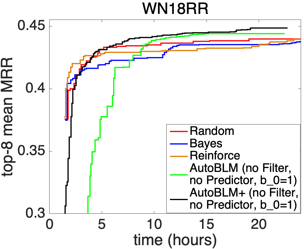
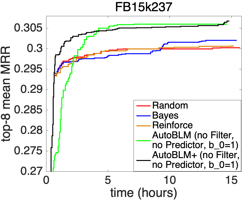
Figure 6: Comparison of different search algorithms.

Figure 6 shows the mean validation MRR of the top $I=8$ structures w.r.t. clock time during the search process. As can be seen, AutoBLM (no Filter, no Predictor, $b_{0}\!\!=\!\!1$) and AutoBLM+ (no Filter, no Predictor, $b_{0}\!\!=\!\!1$) outperform the rest at the later stages. They have poor initial performance as they start with structures having few nonzero elements, which can be degenerate. This will be further demonstrated in the next section.

5.1.5 Ablation Study 2: Effectiveness of the Filter

Structures with more nonzero elements are more likely to satisfy the two conditions in Proposition 2, and thus less likely to be degenerate. Hence, the filter is expected to be particularly useful when there are few nonzero elements in the structure. In this experiment, we demonstrate this by comparing AutoBLM/AutoBLM+ with and without the filter. The performance predictor is always enabled.

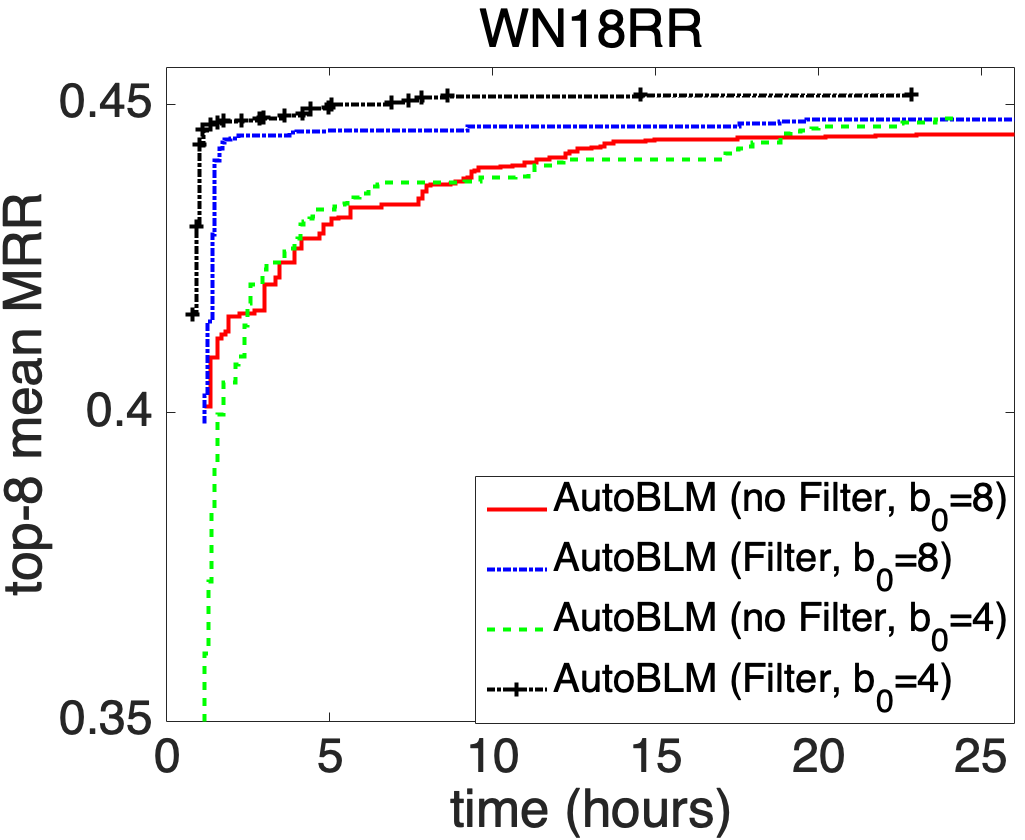
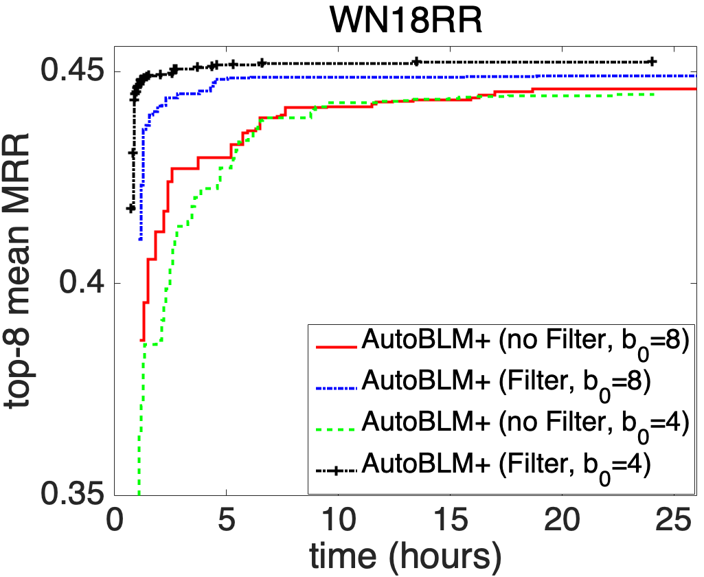
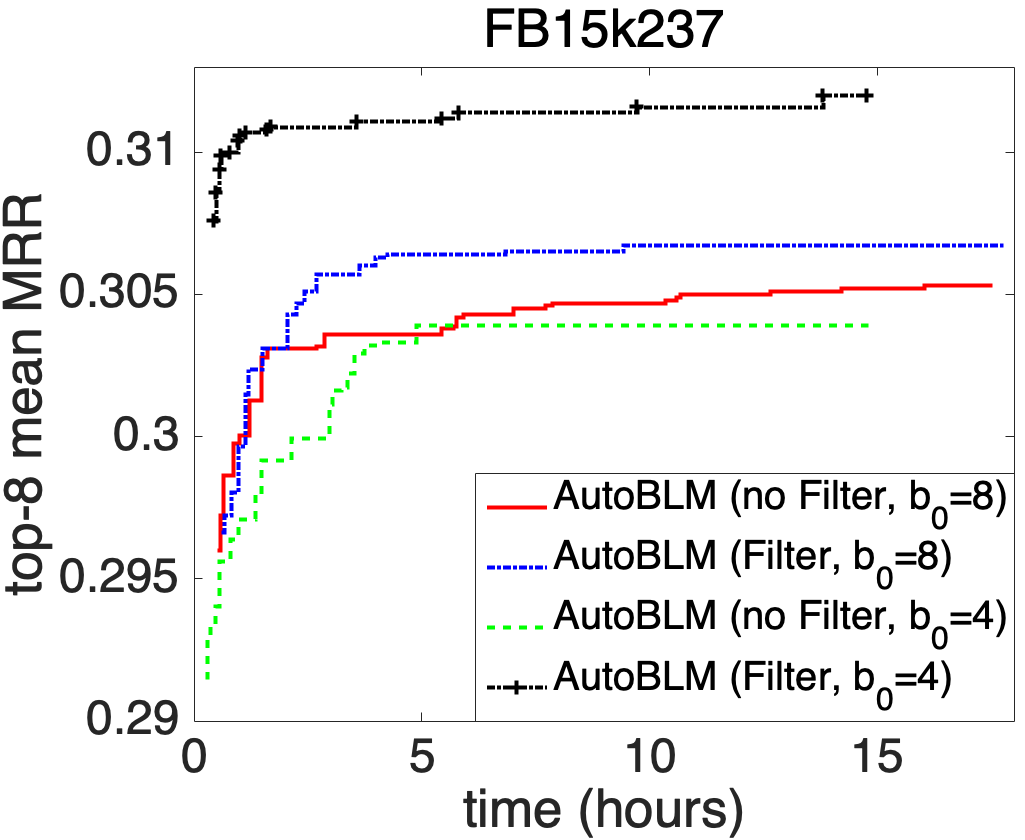
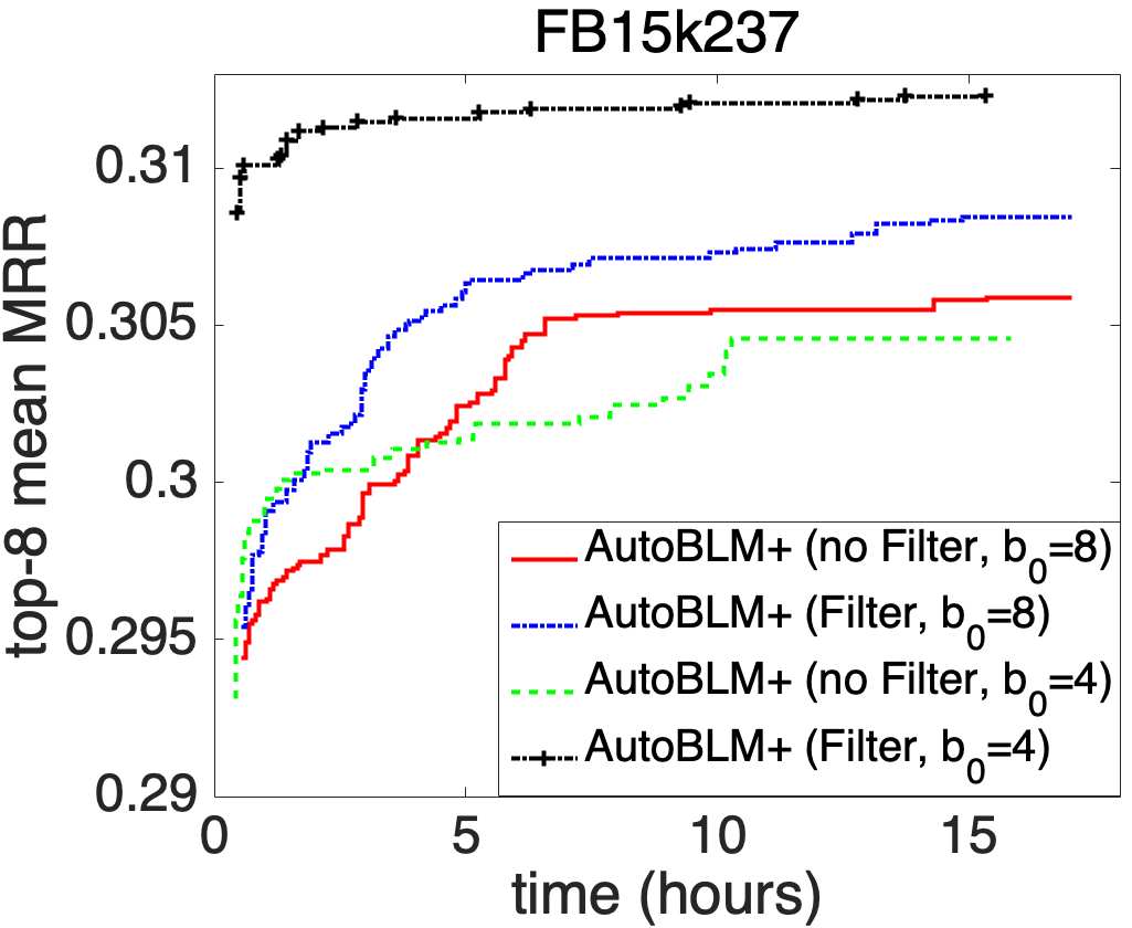
Figure 7: Comparison of the effect of filter.

Figure 7 shows the mean validation MRR of the top $I=8$ structures w.r.t. clock time. As expected, when the filter is not used, using a larger $b_{0}$ will be more likely to have non-degenerate structures and thus better performance, especially at the initial stages. When the filter is used, the performance of both $b_{0}$ settings are improved. In particular, with $b_{0}=4$, the initial search space is simpler and leads to better performance.

5.1.6 Ablation Study 3: Performance Predictor

In this experiment, we compare the following AutoBLM/AutoBLM+ variants: (i) AutoBLM (no-predictor) and AutoBLM+ (no-predictor), which simply randomly select $P$ structures for evaluation (in step 17 of Algorithm 3 and step 16 of Algorithm 4, respectively); (ii) AutoBLM (Predictor+SRF) and AutoBLM+ (Predictor+SRF), using the proposed SRF (in Section 4.2) as input features to the performance predictor; and (iii) AutoBLM (Predictor+1hot) and AutoBLM+ (Predictor+1hot), which map each of the $K^{2}$ entries in $\bm{A}$ (with values in $\{0,\pm 1,\dots,\pm K\}$) to a simple ($2K+1$)-dimensional one-hot vector, and then use these as features to the performance predictor. The resultant feature vector is thus $K^{2}(2K+1)$-dimensional, which is much longer than the $K(K+1)$-dimensional SRF representation.

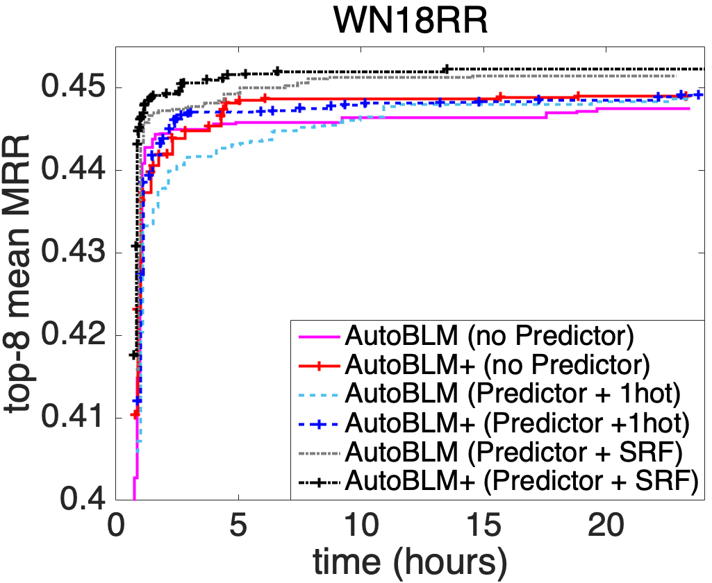
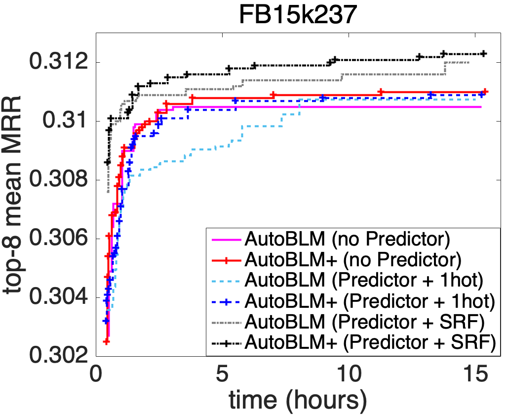
Figure 8: Effectiveness of the performance predictor.

Figure 8 shows the mean validation MRR of the top $I=8$ structures w.r.t. clock time. As can be seen, the use of performance predictor improves the results over AutoBLM (no-Predictor) and AutoBLM+ (no-Predictor). The SRF features also perform better than the one-hot features, as the one-hot features are higher-dimensional and more difficult to learn. Besides, we observe that AutoBLM+ performs better than AutoBLM, as it can more flexibly explore the search space. Thus, in the remaining ablation studies, we will only focus on AutoBLM+.

5.1.7 Ablation Study 4: Varying $K$

As $K$ increases, the search space, which has a size of $(2K+1)^{K^{2}}$ (Section 3.3), increases dramatically. Moreover, the SRF also needs to enumerate a lot more ($K^{2K+1}$) vectors in $\mathcal{C}$. In this experiment, we demonstrate the dependence on $K$ by running AutoBLM+ with $K=3,4,5$. To ensure that $d$ is divisible by $K$, we set $d=60$. Figure 9 shows the top-8 mean MRR performance on the validation set of the searched models versus clock time. As can be seen, the best performance attained by different $K$’s are similar. However, $K=5$ runs slower.

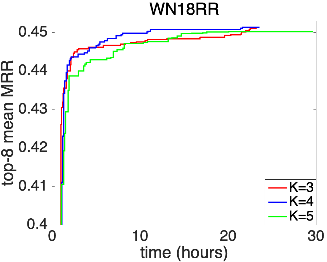
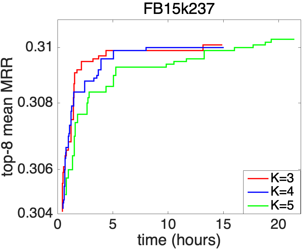
Figure 9: Comparison of different $K$ values.

Table IX shows the running time of the filter, performance predictor (with SRF features), training and evaluation in Algorithm 4 with different $K$’s. As can be seen, the costs of filter and performance predictor increase a lot with $K$, while the model training and evaluation time are relatively stable for different $K$’s.

TABLE IX: Running time (in minutes) of different components in Algorithm 4.

dataset	$K$	filter	performance predictor	train	evaluate
WN18RR	3	0.04	1	1217	152
	4	1.4	23	1231	156
	5	90	276	1252	161
FB15k237	3	0.04	1	714	178
	4	1.5	22	721	181
	5	91	283	728	186

5.1.8 Ablation Study 5: Analysis of Parameter Sharing

As mentioned in Section 4.2, parameter sharing may not reliably predict the model performance. To demonstrate this, we empirically compare the parameter-sharing approach, which shares parameter $\bm{P}=\{\bm{E},\bm{R}\}$ (where $\bm{E}\in\mathbb{R}^{d\times|\mathcal{E}|}$ is the entity embedding matrix and $\bm{R}\in\mathbb{R}^{d\times|\mathcal{R}|}$ is the relation embedding matrix in Section 2.1) and the stand-alone approach, which trains each model separately. For parameter sharing, we randomly sample a $\bm{A}$ in each training iteration from the set of top candidate structures ($\mathcal{H}^{b}$ in Algorithm 3 or $\mathcal{H}$ in Algorithm 4), and then update parameter $\bm{P}$. After one training epoch, the sampled structures are evaluated. After 500 training epochs, the top-100 $\bm{A}$’s are output. For the stand-alone approach, the 100 $\bm{A}$’s are separately trained and evaluated.

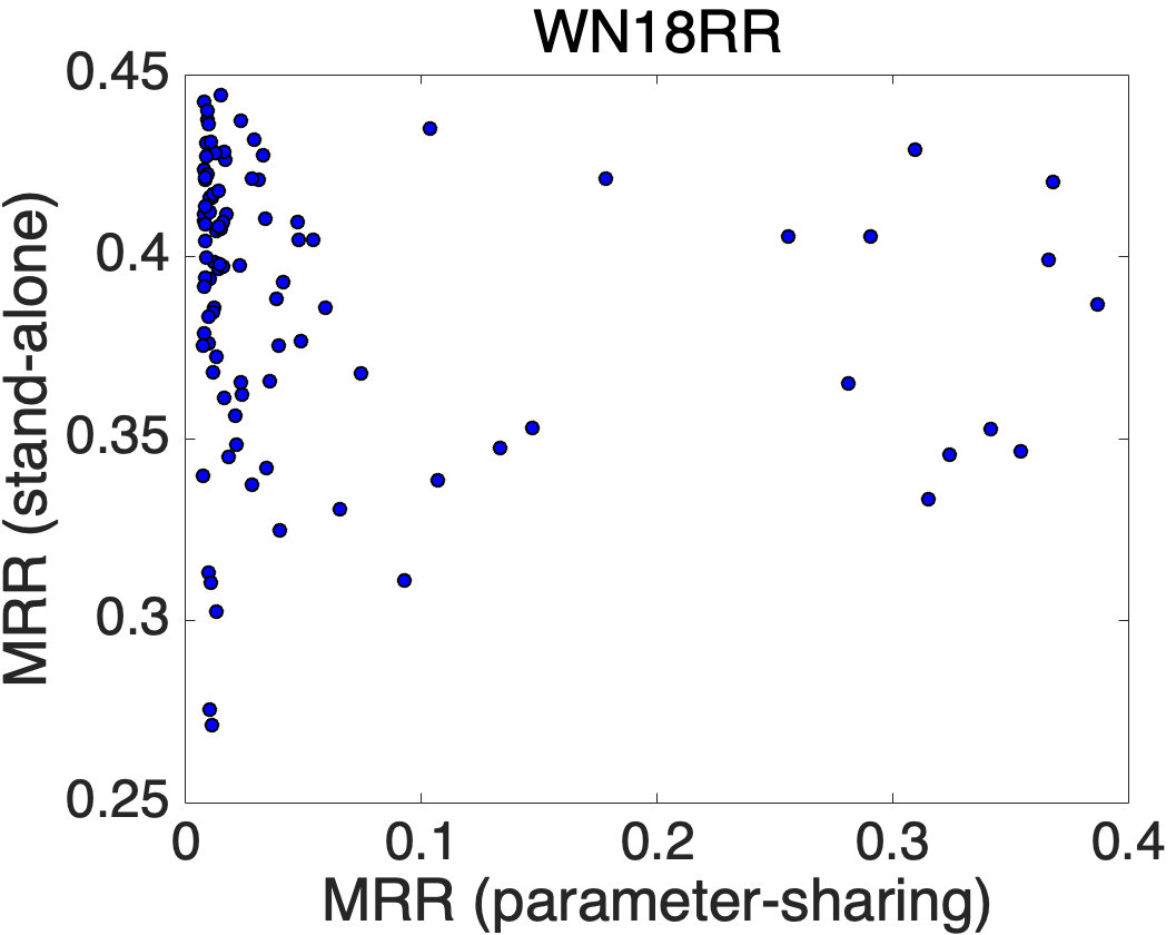
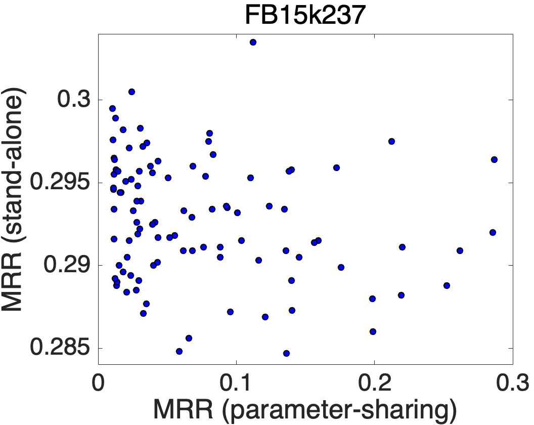
Figure 10: MRRs of structures as estimated by the parameter-sharing approach and stand-alone approach.

Figure 10 shows the MRR estimated by parameter-sharing versus the true MRR obtained by individual model training. As can be seen, structures that have high estimated MRRs (by parameter sharing) do not truly have high MRRs. Indeed, the Spearman’s rank correlation coefficient between the two sets of MRRs is negative ($-0.2686$ on WN18RR and $-0.2451$ on FB15k237). This demonstrates that the one-shot approach, though faster, cannot find good structures.

5.2 Multi-Hop Query

In this section, we perform experiment on multi-hop query as introduced in Section 2.2.2. The entity and relation embeddings are optimized by maximizing the scores on positive queries and minimizing the scores on negative queries, which are generated by replacing $e_{L}$ with an incorrect entity. On evaluation, we rank the scores of queries $(e_{0},r_{1}\circ r_{2}\circ\dots\circ r_{L},e_{L})$ of all $e_{L}\in\mathcal{E}$ to obtain the ranking of ground truth entities.

5.2.1 Setup

Following [4], we use the FB15k and FB15k237 datasets in Table V. Evaluation is based on two-hop (2p) and three-hop (3p) queries. Interested readers are referred to [4] for a more detailed description on query generation. For FB15k, there are 273,710 queries in the training set, 8,000 non-overlapping queries in the validation and testing sets. For FB15k237, there are 143,689 training queries, and 5,000 queries for validation and testing. The setting of the search algorithms’ hyper-parameters are the same as in Section 5.1. For the learning hyper-parameters, we search the dimension $d\in\{32,64\}$, and the other hyper-parameters are the same as those in Section 5.1. We use the MRR performance on the validation set to search for structures as well as hyper-parameters. For performance evaluation, we follow [8, 4], and use the testing Hit@3 and MRR.

We compare with the following baselines: (i) TransE-Comp [39] (based on TransE); (ii) Diag-Comp [39] (based on DistMult); (iii) GQE [8], which uses a $d\times d$ trainable matrix $\bm{R}_{(r)}$ for composition, and can be regarded as a composition based on RESCAL [6]; and (iv) Q2B [4], which is a recently proposed box embedding method.

5.2.2 Results

Results are shown in Table X. As can be seen, among the baselines, TransE-Comp, Diag-Comp and GQE are inferior to Q2B. This shows that the general scoring functions cannot be directly applied to model the complex interactions in multi-hop queries. On the other hand, AutoBLM and AutoBLM+ have better performance as they can adapt to the different tasks with different matrices $g_{K}(\bm{A},\bm{r})$. The obtained structures can be found in Appendix D.

TABLE X: Testing performance of H@3 and MRR on multi-hop query task. Results of $\star$’s are copied from [4].

	FB15K				FB15K237
	2p		3p		2p		3p
	H@3	MRR	H@3	MRR	H@3	MRR	H@3	MRR
TransE-Comp [39]	27.3	.264	15.8	.153	19.4	.177	14.0	.134
Diag-Comp [39]	32.2	.309	27.5	.266	19.1	.187	15.5	.147
GQE [8]$\star$	34.6	.320	25.0	.222	21.3	.193	15.5	.145
Q2B [4]$\star$	41.3	.373	30.3	.274	24.0	.225	18.6	.173
AutoBLM	41.5	.402	29.1	.283	23.6	.232	18.2	.180
AutoBLM+	43.2	.415	30.7	.293	24.9	.248	19.9	.196

5.3 Entity Classification

In this section, we perform experiment on entity classification as introduced in Section 2.2.3.

5.3.1 Setup

After aggregation for $L$ layers, representation $\bm{e}^{L}$ at the last layer is transformed by a multi-layer perception (MLP) to $\bm{e}_{i}^{o}=MLP(\bm{e}_{i}^{L})\in\mathbb{R}^{C}$, where $d$ is the intermediate layer dimension, and is the number of classes. The parameters, including embeddings of entities, relations, $\bm{W}_{0}^{\ell}$, $\bm{W}^{\ell}$’s and the MLP, are optimized by minimizing the cross-entropy loss on the labeled entities: $\mathcal{L}=-\sum_{i\in\mathcal{B}}\sum_{c=1}^{C}y_{ic}\ln e^{o}_{ic}$, where $\mathcal{B}$ is the set of labeled entities, $y_{ic}\in\{0,1\}$ indicates whether the $i$th entity belongs to class $c$, and $e^{o}_{ic}$ is the $c$th dimension of $\bm{e}_{i}^{o}$.

Three graph datasets are used (Table XI): AIFB, an affiliation graph; MUTAG, a bioinformatics graph; and BGS, a geological graph. More details can be found in [68]. All entities do not have attributes. The entities’ and relations’ trainable embeddings are used as input to the GCN.

TABLE XI: Data sets used in entity classification. Sparsity is computed as $\text{\#edges}/(\text{\#entity}^{2}\cdot\text{\#relation})$.

dataset	#entity	#relation	#edges	#train	#test	#classes	sparsity
AIFB	8,285	45	29,043	140	36	4	9.4e-6
MUTAG	23,644	23	74,227	272	68	2	5.7e-6
BGS	333,845	103	916,199	117	29	2	8.0e-8

The following five models are compared: (i) GCN [9], with $\phi(\bm{e}_{j}^{\ell},\bm{r}^{\ell})=\bm{e}_{j}^{\ell}$, does not leverage relations of the edges; (ii) R-GCN [23], with $\phi(\bm{e}_{j}^{\ell},\bm{r}^{\ell})=\bm{R}_{(r)}^{\ell}\bm{e}_{j}^{\ell}$; (iii) CompGCN [24] with $\phi(\bm{e}_{j}^{\ell},\bm{r}^{\ell})=\bm{e}_{j}^{\ell}$ (-/*/$\star$) $\bm{r}^{\ell}$, in which the operator (subtraction/multiplication/circular correlation as discussed in Section 2.2.3) is chosen based on 5-fold cross-validation; (iv) AutoBLM; and (v) AutoBLM+. oth AutoBLM and AutoBLM+ use the searched structure $\bm{A}$ to form $\phi(\bm{e}_{j}^{\ell},\bm{r}^{\ell})=g_{K}(\bm{A},\bm{r}^{\ell})\bm{e}_{j}^{\ell}$.

Setting of the hyper-parameters are the same as in Section 5.1. As for the learning hyper-parameters, we search the embedding dimension $d$ from $\{12,20,32,48\}$, learning rate from $[10^{-5},10^{-1}]$ with Adam as the optimizer [69]. For the GCN structure, the hidden size is the same as the embedding dimension, the dropout rate for each layer is from $[0,0.5]$. We search for 50 hyper-parameter settings for each dataset based on the 5-fold classification accuracy.

For performance evaluation, we use the testing accuracy. Each model runs 5 times, and then the average testing accuracy reported.

5.3.2 Results

Table XII shows the average testing accuracies. Among the baselines, R-GCN is slightly better than CompGCN on the AIFB dataset, but worse on the other two sparser datasets. By searching the composition operators, AutoBLM and AutoBLM+ outperform all the baseline methods. AutoBLM+ is better than AutoBLM since it can find better structures with the same budget by the evolutionary algorithm. The structures obtained are in Appendix D.

TABLE XII: Classification accuracies (in %) on entity classification task. Values marked “*” are copied from [24].

dataset	AIFB	MUTAG	BGS
GCN	86.67	68.83	73.79
R-GCN	92.78	74.12	82.97
CompGCN	90.6∗	85.3∗	84.14
AutoBLM	95.55	85.00	84.83
AutoBLM+	96.66	85.88	86.17

6 Conclusion

In this paper, we propose AutoBLM and AutoBLM+, the algorithms to automatically design and discover better scoring functions for KG learning. By analyzing the limitations of existing scoring functions, we setup the problem as searching relational matrix for BLMs. In AutoBLM, we use a progressive search algorithm which is enhanced by a filter and a predictor with domain-specific knowledge, to search in such a space. Due to the limitation of progressive search, we further design an evolutionary algorithm, enhanced by the same filter and predictor, called AutoBLM+. AutoBLM and AutoBLM+ can efficiently design scoring functions that outperform existing ones on tasks including KG completion, multi-hop query and entity classification from the large search space. Comparing AutoBLM with AutoBLM+, AutoBLM+ can design better scoring functions with the same budget.

Yongqi Zhang (Member, IEEE) is a senior researcher in 4Paradigm. He obtained his Ph.D. degree at the Department of Computer Science and Engineering of Hong Kong University of Science and Technology (HKUST) in 2020 and received his bachelor degree at Shanghai Jiao Tong University (SJTU) in 2015. He has published five top-tier conference/journal papers as first-author, including NeurIPS, ACL, WebConf, ICDE, VLDB-J. His research interests focus on knowledge graph embedding, automated machine learning and graoh learning. He was a Program Committee for AAAI 2020-2022, IJCAI 2020-2022, CIKM 2021, KDD 2022, ICML 2022, and a reviewer for TKDE and NEUNET.

Quanming Yao (Member, IEEE) is a tenure-track assistant professor at Department of Electronic Engineering, Tsinghua University. Before that, he spent three years from a researcher to a senior scientist in 4Paradigm INC, where he set up and led the company’s machine learning research team. He is a receipt of Wunwen Jun Prize of Excellence Youth of Artificial Intelligence (issued by CAAI), the runner up of Ph.D. Research Excellence Award (School of Engineering, HKUST), and a winner of Google Fellowship (in machine learning). Currently, his main research topics are Automated Machine Learning (AutoML) and neural architecture search (NAS). He was an Area Chair for ICLR 2022, IJCAI 2021 and ACML 2021; Senior Program Committee for IJCAI 2020 and AAAI 2020-2021; and a guest editor of IEEE TPAMI AutoML special issue in 2019.

James T. Kwok (Fellow, IEEE) received the Ph.D. degree in computer science from The Hong Kong University of Science and Technology in 1996. He is a Professor with the Department of Computer Science and Engineering, Hong Kong University of Science and Technology. His research interests include machine learning, deep learning, and artificial intelligence. He received the IEEE Outstanding 2004 Paper Award and the Second Class Award in Natural Sciences by the Ministry of Education, China, in 2008. He is serving as an Associate Editor for the IEEE Transactions on Neural Networks and Learning Systems, Neural Networks, Neurocomputing, Artificial Intelligence Journal, International Journal of Data Science and Analytics, Editorial Board Member of Machine Learning, Board Member, and Vice President for Publications of the Asia Pacific Neural Network Society. He also served/is serving as Senior Area Chairs / Area Chairs of major machine learning / AI conferences including NIPS, ICML, ICLR, IJCAI, AAAI and ECML.

Appendix A Proofs

Denote $N=|\mathcal{E}|$. For vectors and matrix, we use the uppercase italic bold letters, such as $\bm{G},\bm{E}$, to denote matrices, use uppercase normal bold letters, such as $\mathbf{G}$, to denote tensors, lowercase bold letters, such as $\bm{r}$ to denote vectors, and normal characters to indicate scalers, such as $K$. $i,j$ are generally used to indicate index. $\bm{E}_{i},\bm{r}_{i},i=1\dots K$, still a matrix or vector, are the $i$-th block of $K$-chunk split, while $r_{i},i=1\dots d$ is a scalar in the $i$-th dimension of vector $\bm{r}$. $\bm{E}_{i,:}$ indicates the $i$-th row of matrix $\bm{E}$, and $\bm{E}_{:,i}$ indicates the $i$-th column. For $g_{K}(\bm{A},\bm{r})\in\mathbb{R}^{d\times d}$, we use $[g_{K}(\bm{A},\bm{r})]_{i,j}$ with $i,j=1\dots K$ to indicate the $(i,j)$-th block, while $\{g_{K}(\bm{A},\bm{r})\}_{i,j}$ with $i,j=1\dots d$ to indicate the element in the $i$-th row and $j$-th column of $g_{K}(\bm{A},\bm{r})$. $\lceil x\rceil$ means the smallest integer that is equal or larger than $x$.

A.1 Proposition 1

Here, we first show some useful lemmas in Appendix A.1.1, then we prove

A.1.1 Auxiliary Lemmas

Recall that

$$\mathcal{C}\equiv\{\bm{r} \in\mathbb{R}^{K}\,|\,\bm{r}\neq\bm{0},$$

$$r_{i}\in\{0,\pm 1,\dots,\pm K\},i=1,\dots,K\}.$$

We firstly show that any symmetric matrix can be factorized as a bilinear form if $\exists\;\hat{\bm{r}}\in\mathcal{C},g_{K}(\bm{A},\hat{\bm{r}})^{\top}=g_{K}(\bm{A},\hat{\bm{r}})$ in Lemma 1; any skew-symmetric matrix can be factorized as a bilinear form if $\exists\;\breve{\bm{r}}\in\mathcal{C},g_{K}(\bm{A},\breve{\bm{r}})^{\top}=-g_{K}(\bm{A},\breve{\bm{r}})$ in Lemma 2.

Lemma 1.

If $\exists\;\hat{\bm{r}}\in\mathcal{C},g_{K}(\bm{A},\hat{\bm{r}})^{\top}=g_{K}(\bm{A},\hat{\bm{r}})$, there exist $\acute{\bm{E}}\in\mathbb{R}^{KN\times N}$ and $\acute{\bm{r}}\in\mathbb{R}^{KN}$ such that any symmetric matrix $\hat{\bm{G}}={\acute{\bm{E}}}^{\top}g_{K}(\bm{A},\acute{\bm{r}})\acute{\bm{E}}$.

Proof.

For any real symmetric matrix $\hat{\bm{G}}\in\mathbb{R}^{N\times N}$, it can be decomposed as [70]

$$\hat{\bm{G}}=\bm{P}^{\top}\bm{\Lambda}\bm{P},$$ (14)

where $\bm{P}\in\mathbb{R}^{N\times N}$ is an orthogonal matrix and $\bm{\Lambda}\in\mathbb{R}^{N\times N}$ is a diagonal matrix with $N$ elements. If $\exists\;\hat{\bm{r}}\in\mathcal{C},g_{K}(\bm{A},\hat{\bm{r}})^{\top}=g_{K}(\bm{A},\hat{\bm{r}})$, we discuss with two cases: 1) there exist some non-zero elements in the diagonal; 2) all the diagonal elements are zero.

To begin with, we evenly split the relation embedding into $K$ parts as $\acute{\bm{r}}=[\acute{\bm{r}}_{1};\acute{\bm{r}}_{2};\dots;\acute{\bm{r}}_{K}]\in\mathbb{R}^{KN}$, and the entity embedding matrix into $K$ blocks as $\acute{\bm{E}}=[\acute{\bm{E}}_{1};\acute{\bm{E}}_{2};\dots;\acute{\bm{E}}_{K}]\in\mathbb{R}^{KN\times N}$. Then for the two cases:

1. If there exist non-zero elements in the diagonal, i.e. $\exists i\in\{1\dots K\}:\;\{g_{K}(\bm{A},\hat{\bm{r}})\}_{i,i}\neq 0$, we denote any one of the index in the diagonal as $(a_{1},a_{1})$ with $a_{1}\in\{1\dots K\}$. Then, we have

   $$\{g_{K}(\bm{A},\hat{\bm{r}})\}_{a_{1},a_{1}}=\text{sign}(A_{a_{1},a_{1}})\cdot\hat{\bm{r}}[|A_{a_{1},a_{1}}|]\neq 0,$$

   and $\text{sign}(A_{a_{1},a_{1}})\neq 0$. Next, we assign $\acute{\bm{E}}$ with

   $$\acute{\bm{E}}_{i}=\begin{cases}\bm{P}&i=a_{1}\\ \bm{0}&\text{otherwise}\end{cases}.$$ (15)

   And $\acute{\bm{r}}$ with

   $$\acute{\bm{r}}_{i}=\begin{cases}\text{sign}(A_{a_{1},a_{1}})\cdot\text{vec}(\bm{\Lambda})&i=|A_{a_{1},a_{1}}|\\ \bm{0}&\text{otherwise}\end{cases},$$ (16)

   where $\text{vec}(\bm{\Lambda})$ returns the diagonal elements in the diagonal matrix $\bm{\Lambda}$ and

   $$[g_{K}(\bm{A},\acute{\bm{r}})]_{a_{1},a_{1}}$$

   $$= \text{sign}(A_{a_{1},a_{1}})\cdot\text{diag}\big{(}\text{sign}(A_{a_{1},a_{1}})\cdot\text{vec}(\bm{\Lambda})\big{)}$$

   $$= \big{(}\text{sign}(A_{a_{1},a_{1}})\big{)}^{2}\cdot\bm{\Lambda}=\bm{\Lambda}.$$ (17)

   Based on (14), (15) and (17), we have

   $${\acute{\bm{E}}}^{\top}g_{K}(\bm{A},\acute{\bm{r}})\acute{\bm{E}}= \sum\nolimits_{i,j}^{K,K}{\acute{\bm{E}}_{i}}^{\top}[g_{K}(\bm{A},\acute{\bm{r}})]_{i,j}\acute{\bm{E}}_{j}$$

   $$= \bm{0}+{\acute{\bm{E}}_{a_{1}}}^{\top}[g_{K}(\bm{A},\acute{\bm{r}})]_{a_{1},a_{1}}\acute{\bm{E}}_{a_{1}},$$

   $$= \bm{0}+\bm{P}^{\top}\bm{\Lambda}\bm{P}=\hat{\bm{G}}.$$

2. If all the diagonal elements are zero, there must be some non-zero elements in the non-diagonal indices, i.e. $\exists(i,j)\in\{1\dots K\}\times\{1\dots K\}:\;\{g_{K}(\bm{A},\hat{\bm{r}})\}_{i,j}\neq 0\wedge i\neq j$. We denote any one of the index in the non-diagonal indices as $(a_{2},a_{3})$ with $a_{2},a_{3}\in\{1\dots K\}$ and $a_{2}\neq a_{3}$. Then we have

   $$\{g_{K}(\bm{A},\hat{\bm{r}})\}_{a_{2},a_{3}} =\{g_{K}(\bm{A},\hat{\bm{r}})\}_{a_{3},a_{2}}$$

   $$=\text{sign}(A_{a_{2},a_{3}})\cdot\hat{\bm{r}}[|A_{a_{2},a_{3}}|]\neq 0,$$

   and $\text{sign}(A_{a_{2},a_{3}})\neq 0$.

   Similarly, we assign $\acute{\bm{E}}$ with

   $$\acute{\bm{E}}_{i}=\begin{cases}\bm{P}&i=a_{2}\text{ or }a_{3}\\ \bm{0}&\text{otherwise}\end{cases}.$$ (18)

   And $\acute{\bm{r}}$ with

   $$\acute{\bm{r}}_{i}=\begin{cases}\frac{\text{sign}(A_{a_{2},a_{3}})}{2}\cdot\text{vec}(\bm{\Lambda})&i=|A_{a_{2},a_{3}}|\\ \frac{\text{sign}(A_{a_{3},a_{2}})}{2}\cdot\text{vec}(\bm{\Lambda})&i=|A_{a_{3},a_{2}}|\\ \bm{0}&\text{otherwise}\end{cases},$$ (19)

   which leads to

   $$[g_{K}(\bm{A},\acute{\bm{r}})]_{a_{2},a_{3}}=[g_{K}(\bm{A},\acute{\bm{r}})]_{a_{3},a_{2}}$$

   $$= {\text{sign}(A_{a_{2},a_{3}})}\cdot\text{diag}\big{(}\frac{\text{sign}(A_{a_{2},a_{3}})}{2}\cdot\text{vec}(\bm{\Lambda})\big{)}$$

   $$= \frac{1}{2}\bm{\Lambda}.$$ (20)

   Based on (14), (18) and (20), we have

   $${\acute{\bm{E}}}^{\top}g_{K}(\bm{A},\acute{\bm{r}})\acute{\bm{E}}=\sum\nolimits_{i,j}^{K,K}{\acute{\bm{E}}_{i}}^{\top}[g_{K}(\bm{A},\acute{\bm{r}})]_{i,j}\acute{\bm{E}}_{j}$$

   $$= \bm{0}+{\acute{\bm{E}}_{a_{2}}}^{\top}[g_{K}(\bm{A},\acute{\bm{r}})]_{a_{2},a_{3}}\acute{\bm{E}}_{a_{3}}+{\acute{\bm{E}}_{a_{3}}}^{\top}[g_{K}(\bm{A},\acute{\bm{r}})]_{a_{3},a_{2}}\acute{\bm{E}}_{a_{2}},$$

   $$= \bm{0}+\bm{P}^{\top}(\frac{1}{2}\bm{\Lambda})\bm{P}+\bm{P}^{\top}(\frac{1}{2}\bm{\Lambda})\bm{P}=\hat{\bm{G}}.$$

Hence, there exist $\acute{\bm{E}}\in\mathbb{R}^{KN\times N}$ and $\acute{\bm{r}}\in\mathbb{R}^{KN}$ such that any symmetric matrix $\hat{\bm{G}}={\acute{\bm{E}}}^{\top}g_{K}(\bm{A},\acute{\bm{r}})\acute{\bm{E}}$. ∎

Lemma 2.

If $\exists\;\breve{\bm{r}}\in\mathcal{C},g_{K}(\bm{A},\breve{\bm{r}})^{\top}=-g_{K}(\bm{A},\breve{\bm{r}})$, there exist $\grave{\bm{E}}\in\mathbb{R}^{KN\times N}$ and $\grave{\bm{r}}\in\mathbb{R}^{KN}$ such that any skew-symmetric matrix $\breve{\bm{G}}={\grave{\bm{E}}}^{\top}g_{K}(\bm{A},\grave{\bm{r}})\grave{\bm{E}}\in\mathbb{R}^{N\times N}$.

Proof.

First, if $\exists\;\breve{\bm{r}}\in\mathcal{C},g_{K}(\bm{A},\breve{\bm{r}})^{\top}=-g_{K}(\bm{A},\breve{\bm{r}})$, all the elements in the diagonal should be zero, i.e. $\{g_{K}(\bm{A},\breve{\bm{r}})\}_{i,j}=0$, with $i=j$. Therefore, there must be some non-zero elements in the non-diagonal indices, i.e., $\exists(i,j)\in\{1\dots K\}^{2}:\;\{g_{K}(\bm{A},\breve{\bm{r}})\}_{i,j}\neq 0\wedge i\neq j$. We denote any one of the index in the non-diagonal indices as $(b_{1},b_{2})$ with $b_{1},b_{2}\in\{1\dots K\}$ and $b_{1}\neq b_{2}$. Then we have

$$\{g_{K}(\bm{A},\breve{\bm{r}})\}_{b_{1},b_{2}} =-\{g_{K}(\bm{A},\breve{\bm{r}})\}_{b_{2},b_{1}}$$

$$=\text{sign}(A_{b_{1},b_{2}})\cdot\breve{\bm{r}}[|A_{b_{1},b_{2}}|]\neq 0,$$

and $\text{sign}(A_{b_{1},b_{2}})\neq 0$. Next, we assign $\acute{\bm{E}}$ with

$$\grave{\bm{E}}_{i}=\begin{cases}\bm{I}&i=b_{1}\\ \breve{\bm{G}}&i=b_{2}\\ \bm{0}&\text{otherwise}\end{cases}.$$ (21)

And $\acute{\bm{r}}$ with

$$\grave{\bm{r}}_{i}=\begin{cases}\frac{\text{sign}(A_{b_{1},b_{2}})}{2}\cdot\bm{1}&i=|A_{b_{1},b_{2}}|\\ \frac{\text{sign}(A_{b_{2},b_{1}})}{2}\cdot\bm{1}&i=|A_{b_{2},b_{1}}|\\ \bm{0}&\text{otherwise}\end{cases},$$ (22)

which leads to

$$[g_{K}(\bm{A},\grave{\bm{r}})]_{b_{1},b_{2}}=-[g_{K}(\bm{A},\grave{\bm{r}})]_{b_{2},b_{1}}$$

$$= {\text{sign}(A_{b_{1},b_{2}})}\cdot\text{diag}\big{(}\frac{\text{sign}(A_{b_{1},b_{2}})}{2}\cdot{\bm{1}}\big{)}$$

$$= \frac{1}{2}\bm{I}.$$ (23)

Since $\breve{\bm{G}}$ is skew-symmetric, we have

$$\breve{\bm{G}}^{\top}=-\breve{\bm{G}}.$$ (24)

Based on (21), (23) and (24) we have

$${\grave{\bm{E}}}^{\top}g_{K}(\bm{A},\grave{\bm{r}})\grave{\bm{E}}=\sum\nolimits_{i,j}^{K,K}{\grave{\bm{E}}_{i}}^{\top}[g_{K}(\bm{A},\grave{\bm{r}})]_{i,j}\grave{\bm{E}}_{j}$$

$$= \bm{0}+{\grave{\bm{E}}_{b_{1}}}^{\top}[g_{K}(\bm{A},\grave{\bm{r}})]_{b_{1},b_{2}}\grave{\bm{E}}_{b_{2}}+{\grave{\bm{E}}_{b_{2}}}^{\top}[g_{K}(\bm{A},\grave{\bm{r}})]_{b_{2},b_{1}}\grave{\bm{E}}_{b_{1}},$$

$$= \bm{0}+\bm{I}^{\top}(\frac{1}{2}\bm{I})\breve{\bm{G}}+\breve{\bm{G}}^{\top}(-\frac{1}{2}\bm{I})\bm{I}$$

$$= \bm{0}+\frac{1}{2}\breve{\bm{G}}-\frac{1}{2}(-\breve{\bm{G}})=\breve{\bm{G}}.$$

Hence, there exist $\grave{\bm{E}}\in\mathbb{R}^{KN\times N}$ and $\grave{\bm{r}}\in\mathbb{R}^{KN}$ such that any symmetric matrix $\breve{\bm{G}}={\grave{\bm{E}}}^{\top}g_{K}(\bm{A},\grave{\bm{r}})\grave{\bm{E}}$. ∎

Based on Lemma 1 and 2, we prove the following lemma for any real-valued square matrices.

Lemma 3.

If 1) $\exists\;\hat{\bm{r}}\in\mathcal{C},g_{K}(\bm{A},\hat{\bm{r}})^{\top}=g_{K}(\bm{A},\hat{\bm{r}})$), and 2) $\exists\;\breve{\bm{r}}\in\mathcal{C},g_{K}(\bm{A},\breve{\bm{r}})^{\top}=-g_{K}(\bm{A},\breve{\bm{r}})$), then there exist $\bm{E}\in\mathbb{R}^{2KN\times N}$ and $\bm{r}\in\mathbb{R}^{2KN}$ that any matrix $\bm{G}\in\mathbb{R}^{N\times N}$ can be written as

$$G_{ht}=f(h,r,t)=\bm{h}^{\top}g_{K}(\bm{A},\bm{r})\bm{t},$$

where $\bm{h}=\bm{E}_{:,h}$, $\bm{t}=\bm{E}_{:,t}$.

Proof.

In Lemma 1 and Lemma 2, we prove that any symmetric matrix can be factorized as $\hat{\bm{G}}={\acute{\bm{E}}}^{\top}g_{K}(\bm{A},\acute{\bm{r}})\acute{\bm{E}}$ with $\acute{\bm{E}}\in\mathbb{R}^{KN\times N}$ and $\acute{\bm{r}}\in\mathbb{R}^{KN}$ and any skew-symmetric matrix can be factorized as $\breve{\bm{G}}={\grave{\bm{E}}}^{\top}g_{K}(\bm{A},\grave{\bm{r}})\grave{\bm{E}}\in\mathbb{R}^{N\times N}$ with $\grave{\bm{E}}\in\mathbb{R}^{KN\times N}$ and $\grave{\bm{r}}\in\mathbb{R}^{KN}$. In this part, we show any square matrix $\bm{G}$ can be split as the sum of a particular $\hat{\bm{G}}$ and a particular $\breve{\bm{G}}$ and it can be factorized in the bilinear form with the composition of $\acute{\bm{E}},\grave{\bm{E}}$ and $\acute{\bm{r}},\grave{\bm{r}}$.

We firstly composite $\acute{\bm{E}},\acute{\bm{r}}$ in the proof of Lemma 1 and $\grave{\bm{E}},\grave{\bm{r}}$ in the proof of Lemma 2 into $\bm{E}\in\mathbb{R}^{2KN\times N}$ and $\bm{r}\in\mathbb{R}^{2KN}$. The basic idea is to add the symmetric part into odd rows and skew-symmetric part into even rows. Specifically, we define the rows of $\bm{E}$ as

$$\bm{E}_{i,:}=\begin{cases}\acute{\bm{E}}_{\frac{i+1}{2},:}&i\textit{\,mod\,}2=1\\ \grave{\bm{E}}_{\frac{i}{2},:}&i\textit{\,mod\,}2=0\end{cases}.$$ (25)

And the relation embedding $\bm{r}$ is element-wise set as

$$\bm{r}[i]=\begin{cases}\acute{\bm{r}}[{\frac{i+1}{2},:}]&i\textit{\,mod\,}2=1\\ \grave{\bm{r}}[{\frac{i}{2},:}]&i\textit{\,mod\,}2=0\end{cases}.$$ (26)

Based on the form of $\bm{r}$ we can have $g_{K}(\bm{A},\bm{r})\in\mathbb{R}^{2KN\times 2KN}$ where each element is formed by corresponding element in $g_{K}(\bm{A},\acute{\bm{r}})$ or $g_{K}(\bm{A},\grave{\bm{r}})$ as

$$\!\!\!\{g_{K}(\bm{A},\bm{r})\}_{i,j}$$

$$\!\!\!= \begin{cases}\{g_{K}(\bm{A},\acute{\bm{r}})\}_{\frac{i+1}{2},\frac{j+1}{2}},&\!\!\!\!i\textit{\,mod\,}2=1\text{ and }j\textit{\,mod\,}2=1\\ \{g_{K}(\bm{A},\grave{\bm{r}})\}_{\frac{i}{2},\frac{j}{2}},&\!\!\!\!i\textit{\,mod\,}2=0\text{ and }j\textit{\,mod\,}2=0\\ 0&\!\!\!\!\text{otherwise}.\end{cases}.$$ (27)

Refer to the notation introduced at the beginning of Appendix A, $\{g_{K}(\bm{A},\bm{r})\}_{i,j}$ represents the $(i,j)$-th element in the matrix, while $[g_{K}(\bm{A},\bm{r})]_{i,j}$ represents the $(i,j)$-th block in previous parts. Note that such a construction of $g_{K}(\bm{A},\bm{r})$ will not violate the structure matrix $\bm{A}$. The construction of (25), (26) are graphically illustrated in the left part of Figure 11, which leads to the construction of (27) in the right part.

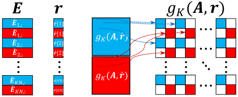
Figure 11: Graphical illustration of the composed embeddings. The blue parts are from $\acute{\bm{E}}$, $\acute{\bm{r}}$ or $g_{K}(\bm{A},\acute{\bm{r}})$ and the red parts are from $\grave{\bm{E}}$, $\grave{\bm{r}}$ or $g_{K}(\bm{A},\grave{\bm{r}})$. The white spaces in $g_{K}(\bm{A},\bm{r})$ are zero values.

Given any matrix $\bm{G}\in\mathbb{R}^{N\times N}$, it can be split into a symmetric part $\hat{\bm{G}}$ and a skew-symmetric part $\breve{\bm{G}}$, i.e.,

$$\bm{G}=\underbrace{\frac{\bm{G}+\bm{G}^{\top}}{2}}_{\hat{\bm{G}}}+\underbrace{\frac{\bm{G}-\bm{G}^{\top}}{2}}_{\breve{\bm{G}}}.$$ (28)

Based on (25), (26), (27), and (28), $\forall h,t$, we have

$$G_{ht}= [\hat{G}]_{ht}\!+\![\breve{G}]_{ht}\!=\!{\acute{\bm{E}}_{:,h}}^{\top}g_{K}(\bm{A},\acute{\bm{r}})\acute{\bm{E}}_{:,t}\!+\!{\grave{\bm{E}}_{:,h}}^{\top}g_{K}(\bm{A},\grave{\bm{r}})\grave{\bm{E}}_{:,t},$$

$$= \sum\nolimits_{m,n}^{KN}\acute{E}_{m,h}\{g_{K}(\bm{A},\acute{\bm{r}})\}_{m,n}\acute{E}_{n,t}+0$$ (29)

$$+0+\sum\nolimits_{m,n}^{KN}\grave{E}_{m,h}\{g_{K}(\bm{A},\grave{\bm{r}})\}_{m,n}\grave{E}_{n,t}$$ (30)

$$= \sum\nolimits_{(i,j)\textit{\,mod\,}2=(1,1)}^{2KN,2KN}E_{i,h}\{g_{K}(\bm{A},\bm{r})\}_{i,j}E_{j,t}$$ (31)

$$+\sum\nolimits_{(i,j)\textit{\,mod\,}2=(1,0)}^{2KN,2KN}E_{i,h}\{g_{K}(\bm{A},\bm{r})\}_{i,j}E_{j,t}$$ (32)

$$+\sum\nolimits_{(i,j)\textit{\,mod\,}2=(0,1)}^{2KN,2KN}E_{i,h}\{g_{K}(\bm{A},\bm{r})\}_{i,j}E_{j,t}$$ (33)

$$+\sum\nolimits_{(i,j)\textit{\,mod\,}2=(0,0)}^{2KN,2KN}E_{i,h}\{g_{K}(\bm{A},\bm{r})\}_{i,j}E_{j,t}$$ (34)

$$= \sum\nolimits_{i,j}^{2KN,2KN}E_{i,h}\{g_{K}(\bm{A},\bm{r})\}_{i,j}E_{j,t}$$

$$= {\bm{E}_{:,h}}^{\top}g_{K}(\bm{A},\bm{r})\bm{E}_{:,t}=\bm{h}^{\top}g_{K}(\bm{A},\bm{r})\bm{t}=f(h,r,t),$$

with $\bm{h}=\bm{E}_{:,h},\bm{t}=\bm{E}_{:,t}$ and $\bm{r}$ in (26). (32) and (33) are 0 since $\{g_{K}(\bm{A},\bm{r})\}_{i,j}$ is zero when $i$ and $j$ are not simultaneously even or odd. From (29) to (31), we let $m=\nicefrac{{i+1}}{{2}}$ and $n=\nicefrac{{j+1}}{{2}}$ to get the odd part in (25) and (27). From (30) to (34), we let $m=\nicefrac{{i}}{{2}}$ and $n=\nicefrac{{j}}{{2}}$ to obtain the even part in (25) and (27). ∎

Finally, we show a Lemma which bridges 3 order tensor $\mathbf{G}$ with bilinear scoring function of form (7). Given any KG with tensor form $\mathbf{G}\in\mathbb{R}^{|\mathcal{E}|\times|\mathcal{R}|\times|\mathcal{E}|}$, we denote $\bm{G}_{r}\in\mathbb{R}^{\mathcal{E}\times\mathcal{E}}$ as the $r$-th slice in the lateral of $\mathbf{G}$, i.e. $\bm{G}_{r}=\mathbf{G}_{\cdot,r,\cdot}$, corresponding to relation $r$.

Lemma 4.

Given any KG with tensor form $\mathbf{G}\in\mathbb{R}^{|\mathcal{E}|\times|\mathcal{R}|\times|\mathcal{E}|}$, and structure matrix $\bm{A}$. If all the $\bm{G}_{r}$’s can be independently expressed by a unique entity embedding matrices $\dot{\bm{E}}_{r}\in\mathbb{R}^{2KN\times N}$ and relation embedding $\dot{\bm{r}}\in\mathbb{R}^{2KN}$, i.e. $\forall h,t=1\dots N,[G_{r}]_{h,t}=\dot{\bm{h}}_{r}^{\top}g_{K}(\bm{A},\dot{\bm{r}}_{r})\dot{\bm{t}}_{r}$, with $\dot{\bm{h}}_{r}=[\dot{\bm{E}}_{r}]_{\cdot,h},\dot{\bm{t}}_{r}=[\dot{\bm{E}}_{r}]_{\cdot,t}$, then there exist entity embedding $\bm{E}\in\mathbb{R}^{2KN|\mathcal{R}|\times N}$ and relation embedding $\bm{R}\in\mathbb{R}^{2KN|\mathcal{R}|\times|\mathcal{R}|}$ such that $\forall h,r,t,G_{hrt}=f_{\bm{A}}(h,r,t)=\bm{h}^{\top}g_{K}(\bm{A},\bm{r})\bm{t}$.

Proof.

We show that computing $G_{hrt}$ can be independently expressed by $[G_{r}]_{ht}$ for each relation $r$. Specifically, we define the rows of entity embedding in $\bm{E}$ as

$$\bm{E}_{i,:}=[\dot{\bm{E}}_{i\textit{\,mod\,}|\mathcal{R}|}]_{\lceil\frac{i}{|\mathcal{R}|}\rceil,:}$$ (35)

And each element in the relation embedding $\bm{r}$ as

$$\bm{r}[i]=\begin{cases}\dot{\bm{r}}[r]_{\lceil\frac{i}{|\mathcal{R}|}\rceil}&i\textit{\,mod\,}\mathcal{R}=r\\ 0&\text{otherwise},\end{cases},$$ (36)

which leads to the element in $g_{K}(\bm{A},\bm{r})$ as

$$\{g_{K}(\bm{A},\bm{r})\}_{i,j}$$

$$=\begin{cases}\{g_{K}(\bm{A},\dot{\bm{r}}_{r})\}_{\lceil\frac{i}{|\mathcal{R}|}\rceil,\lceil\frac{j}{|\mathcal{R}|}\rceil}&i\textit{\,mod\,}|\mathcal{R}|=r\textit{\;and\;}j\textit{\,mod\,}|\mathcal{R}|=r\\ 0&\text{otherwise}\end{cases}.$$ (37)

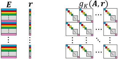
Figure 12: Graphical illustration of the composed embeddings. Different colors represent components from different embeddings. White colors mean the zero values and gray colors represent spaces with mixed colors.

The construction of (35), (36) and (37) can be graphically illustrated in Figure 12. Under these definitions, we can get that each element $G_{hrt}$ can be expressed with

$$G_{hrt} =[G_{r}]_{h,t}$$

$$=\sum_{i_{r}=1}^{2K|\mathcal{E}|}\sum_{j_{r}=1}^{2K|\mathcal{E}|}[E_{r}]_{i_{r},h}\{g_{K}(\bm{A},\bm{r}_{r})\}_{i_{r},j_{r}}[E_{r}]_{j_{r},t}$$ (38)

$$=\sum_{i=1}^{|\mathcal{R}|\cdot 2K|\mathcal{E}|}\sum_{j=1}^{|\mathcal{R}|\cdot 2K|\mathcal{E}|}E_{ih}\{g_{K}(\bm{A},\bm{r})\}_{ij}E_{jt}$$ (39)

$$=\bm{h}^{\top}g_{K}(\bm{A},\bm{r})\bm{t}$$

The step to get (38) depends on Lemma 3. Eq. (38) to (39) depends on (35) and (37). ∎

A.1.2 Proof of Proposition 1

Proof.

Based on Lemma 3 and Lemma 4, if

1. $\exists\hat{\bm{r}}\in\mathcal{C}$ such that $g_{K}(\bm{A},\hat{\bm{r}})$ is symmetric, and

2. $\exists\breve{\bm{r}}\in\mathcal{C}$ such that $g_{K}(\bm{A},\breve{\bm{r}})$ is skew-symmetric,

with $\mathcal{C}\equiv\{\bm{r}\in\mathbb{R}^{K}\,|\,\bm{r}\neq\bm{0},r_{i}\in\{0,\pm 1,\dots,\pm K\},i=1,\dots,K\},$, then given any KG with the tensor form $\mathbf{G}$, there exist entity embedding $\bm{E}\in\mathbb{R}^{2K|\mathcal{E}||\mathcal{R}|\times|\mathcal{E}|}$ and relation embedding $\bm{R}\in\mathbb{R}^{2K|\mathcal{E}||\mathcal{R}|\times|\mathcal{R}|}$ such that for all $h,r,t$, we have

$$G_{hrt}=f_{\bm{A}}(h,r,t)=\bm{h}^{\top}g_{K}(\bm{A},\bm{r})\bm{t},$$

with $\bm{h}=\bm{E}_{:,h},\bm{t}=\bm{E}_{:,t},\bm{r}=\bm{E}_{:,r}$. Thus, scoring function (7) is fully expressive once condition 1) and 2) hold. ∎

A.2 Proposition 2

A.2.1 Auxiliary Lemmas

First, we introduce two lemmas from matrix theory about the rank of Kronecker product and the solution of equation group.

Lemma 5 ([70]).

Denote $\otimes$ as the Kronecker product, given two matrices $\bm{X},\bm{Y}$, we have $\text{rank}(\bm{X}\otimes\bm{Y})=\text{rank}(\bm{X})\cdot\text{rank}(\bm{Y})$.

Lemma 6 ([70]).

Given $\bm{A}\in\mathbb{R}^{d\times d}$, there is no non-zero solution $\bm{x}\neq\bm{0}\in\mathbb{R}^{d}$ for the equation group $\bm{A}\bm{x}=\bm{0}$, if and only if $\text{rank}(\bm{A})=d$.

Note that the definition of degenerate structure $\bm{A}$ is that $\exists\bm{h}\neq 0,\bm{h}^{\top}g_{K}(\bm{A},\bm{r})\bm{t}\neq 0,\forall\bm{r},\bm{t}$ or $\exists\bm{r}\neq 0,\bm{h}^{\top}g_{K}(\bm{A},\bm{r})\bm{t}=0,\forall\bm{h},\bm{t}$. To proof that $\bm{A}$ is not degenerate if and only if $\emph{rank}(\bm{A})=K$ and $\{1,\dots,K\}\subset\{|A_{ij}|:i,j=1\dots K\}$, we prove its converse-negative proposition in Lemma 7.

Lemma 7.

$\exists\bm{h}\neq 0,\bm{h}^{\top}g_{K}(\bm{A},\bm{r})\bm{t}\neq 0,\forall\bm{r},\bm{t}$ or $\exists\bm{r}\neq 0,\bm{h}^{\top}g_{K}(\bm{A},\bm{r})\bm{t}=0,\forall\bm{h},\bm{t}$. if and only if $\text{rank}(\bm{A})<K$ or $\exists a\in\{1,\dots,K\},a\notin\{|A_{ij}|:,i,j=1\dots K\}$.

This can be decomposed into two separate parts in Lemma 8 and 9.

Lemma 8.

$\exists\bm{h}\neq 0,\bm{h}^{\top}g_{K}(\bm{A},\bm{r})\bm{t}\neq 0,\forall\bm{r},\bm{t}$ if and only if $\text{rank}(\bm{A})<K$.

Proof.

To begin with, we show the relationship between the rank of $g_{K}(\bm{A},\bm{r})$ and the rank of $\bm{A}$. If we assign $\bm{r}=\bm{1}\in\mathbb{R}^{d}$, then the $(i,j)$-th block will be $[\bm{g}_{K}(\bm{A},\bm{1})]_{ij}=\text{sign}(A_{ij})\cdot\bm{I}$ with the identity matrix $\bm{I}\in\mathbb{R}^{\frac{d}{K}\times\frac{d}{K}}$. Using Kronecker product, we can write $\bm{g}_{K}(\bm{A},\bm{1})$ as a Kronecker product,

$$\bm{g}_{K}(\bm{A},\bm{1})=\text{sign}(\bm{A})\otimes\bm{I},$$ (40)

where $\otimes$ here represents the Kronercker product and $\text{sign}(\bm{A})$ is a $K\times K$ matrix formed by the signs of elements in $\bm{A}$. Then, based on Lemma 5, we have

$$\text{rank}\big{(}\bm{g}_{K}(\bm{A},\bm{1})\big{)}=\nicefrac{{d}}{{K}}\cdot\text{rank}(\bm{A}),$$ (41)

and $\forall\bm{r}\in\mathbb{R}^{d}$, $\text{rank}\big{(}\bm{g}_{K}(\bm{A},\bm{r})\big{)}\leq\nicefrac{{d}}{{K}}\cdot\text{rank}(\bm{A})$.

• First, we show the sufficient condition, i.e., if $\text{rank}(\bm{A})<K$, we have $\exists\bm{h}\neq 0,\bm{h}^{\top}g_{K}(\bm{A},\bm{r})\bm{t}\neq 0,\forall\bm{r},\bm{t}$.

  Since $\bm{A}$ is not full rank, we have $\text{rank}\big{(}\bm{g}_{K}(\bm{A},\bm{r})\big{)}<d$ based on (41). Then based on Lemma 6, for all $\bm{r}\in\mathbb{R}^{d}$ there exists $\bm{h}\neq\bm{0}$ that

  $$\bm{g}_{K}(\bm{A},\bm{r})^{\top}\bm{h}=\bm{0}.$$

  This leads to $\bm{h}^{\top}\bm{g}_{K}(\bm{A},\bm{r})=\bm{0}$. Thus, if $\text{rank}(\bm{A})<K$, $\exists\bm{h}\neq\bm{0},\forall\bm{r},\bm{t},\bm{h}^{\top}\bm{g}_{K}(\bm{A},\bm{r})\bm{t}=0$.

• Then we show the necessary condition, i.e., if $\exists\bm{h}\neq 0,\bm{h}^{\top}g_{K}(\bm{A},\bm{r})\bm{t}\neq 0,\forall\bm{r},\bm{t}$, we have $\text{rank}(\bm{A})<K$.

  We assign $\bm{r}=\bm{1}$, and a set of $\bm{t}$ with $(1,0,\dots,0),(0,1,\dots,0),\dots,(0,0,\dots,1)$. Then, this will lead to the following equation group

  $$\bm{h}^{\top}\{\bm{g}_{K}(\bm{A},\bm{1})\}_{\cdot,1} =0,$$

  $$\bm{h}^{\top}\{\bm{g}_{K}(\bm{A},\bm{1})\}_{\cdot,2} =0,$$

  $$\cdots,$$

  $$\bm{h}^{\top}\{\bm{g}_{K}(\bm{A},\bm{1})\}_{\cdot,d} =0.$$

  We proof the necessary condition by contraction here. Assume $\text{rank}(\bm{A})=K$, then $\text{rank}\big{(}\bm{g}_{K}(\bm{A},\bm{1})^{\top}\big{)}=\text{rank}\big{(}\bm{g}_{K}(\bm{A},\bm{1})\big{)}=d$ based on (40). Then, based on Lemma 6, there is no $\bm{h}\neq\bm{0}$ such that the above equation group is satisfied. Thus, the assumption that $\text{rank}(\bm{A})=K$ is wrong. Therefore, if $\exists\bm{h}\neq 0,\bm{h}^{\top}g_{K}(\bm{A},\bm{r})\bm{t}\neq 0,\forall\bm{r},\bm{t}$, we have $\text{rank}(\bm{A})<K$.

Based on the proof of sufficient and necessary conditions, we have $\exists\bm{h}\neq 0,\bm{h}^{\top}g_{K}(\bm{A},\bm{r})\bm{t}\neq 0,\forall\bm{r},\bm{t}$ if and only if $\text{rank}(\bm{A})<K$. ∎

Lemma 9.

$\exists\bm{r}\neq 0,\bm{h}^{\top}g_{K}(\bm{A},\bm{r})\bm{t}=0,\forall\bm{h},\bm{t}$ if and only if $\exists a\in\{1,\dots,K\},a\notin\{|A_{ij}|:,i,j=1\dots K\}$.

Proof.

• First, we show the sufficient condition, i.e., if $\exists a\in\{1,\dots,K\},a\notin\{|A_{ij}|:,i,j=1\dots K\}$, we have $\exists\bm{r}\neq 0,\bm{h}^{\top}g_{K}(\bm{A},\bm{r})\bm{t}=0,\forall\bm{h},\bm{t}$.

  Given the $K$-chunk representation of $\bm{r}$, if $\exists$ $a$ $\in$ $\{1,\dots,K\},a\notin\{|A_{ij}|:,i,j=1\dots K\}$, we assign

  $$\bm{r}_{i}=\begin{cases}\bm{1}&i=a\\ \bm{0}&i\neq a\end{cases}.$$ (42)

  Then, $\bm{r}_{|A_{ij}|}=\bm{0}$ is always true since $|A_{ij}|\neq a$. This leads to $g_{K}(\bm{A},\bm{r})=\bm{0}$ with $[g_{K}(\bm{A},\bm{r})]_{ij}=\text{sign}(A_{ij})\cdot\text{diag}\!\left((\bm{r}_{|A_{ij}|})\right)=\bm{0}$. As a result, $\forall\bm{h},\bm{t},\bm{h}^{\top}g_{K}(\bm{A},\bm{r})\bm{t}=0$. Therefore, if $\exists a\in\{1,\dots,K\},a\notin\{|A_{ij}|:,i,j=1\dots K\}$, we have $\exists\bm{r}\neq 0,\bm{h}^{\top}g_{K}(\bm{A},\bm{r})\bm{t}=0,\forall\bm{h},\bm{t}$.

• Then, we show the necessary condition, i.e., if $\exists\bm{r}\neq 0,\bm{h}^{\top}g_{K}(\bm{A},\bm{r})\bm{t}=0,\forall\bm{h},\bm{t}$, we have $\exists a\in\{1,\dots,K\},a\notin\{|A_{ij}|:,i,j=1\dots K\}$.

  We can enumerate $\bm{h},\bm{t}$ as the set of unit vectors with one dimension as $1$ and the remaining to be $0$. Then from $\bm{h}^{\top}g_{K}(\bm{A},\bm{r})\bm{t}=0$ we derive $g_{K}(\bm{A},\bm{r})=\bm{0}$ since any element is $0$. Specially, we have that each block in $g_{K}(\bm{A},\bm{r})$ is

  $$[g_{K}(\bm{A},\bm{r})]_{ij}=\text{sign}(A_{ij})\cdot\text{diag}\!\left((\bm{r}_{|A_{ij}|})\right)=\bm{0}.$$

  If the number of unique values of set $\{A_{ij}\}$ is $K$, we will have $\bm{r}=0$. This is in contrary to the fact that $\bm{r}\neq\bm{0}$. Thus there must $\exists a\in\{1,\dots,K\},a\notin\{|A_{ij}|:,i,j=1\dots K\}$.

Thus, we have $\exists\bm{r}\neq 0,\bm{h}^{\top}g_{K}(\bm{A},\bm{r})\bm{t}=0,\forall\bm{h},\bm{t}$ if and only if $\exists a\in\{1,\dots,K\},a\notin\{|A_{ij}|:,i,j=1\dots K\}$. ∎

By combining Lemma 8 and Lemma 9, we can show Lemma 7 that $\exists\bm{h}\neq 0,\bm{h}^{\top}g_{K}(\bm{A},\bm{r})\bm{t}\neq 0,\forall\bm{r},\bm{t}$ or $\exists\bm{r}\neq 0,\bm{h}^{\top}g_{K}(\bm{A},\bm{r})\bm{t}=0,\forall\bm{h},\bm{t}$. if and only if $\text{rank}(\bm{A})<K$ or $\exists a\in\{1,\dots,K\},a\notin\{|A_{ij}|:,i,j=1\dots K\}$. Since the original statement is equal to the converse-negative proposition, Proposition 2 is proved.

A.2.2 Proof of Proposition 2

Proof.

Proposition 2, is equivalent to the statement that $\bm{A}$ is degenerate if and only if $\text{rank}(\bm{A})<K$ and $\exists a\in\{1,\dots,K\},a\notin\{|A_{ij}|:,i,j=1\dots K\}$. From Definition 5, $\bm{A}$ is degenerate means

1. $\exists\bm{h}\neq 0,\bm{h}^{\top}g_{K}(\bm{A},\bm{r})\bm{t}\neq 0,\forall\bm{r},\bm{t}$; or

2. $\exists\bm{r}\neq 0,\bm{h}^{\top}g_{K}(\bm{A},\bm{r})\bm{t}=0,\forall\bm{h},\bm{t}$.

Here, Lemma 8 proves 1) and Lemma 9 proves 2). Thus, we can conclude that $\bm{A}$ is non-degenerate, if and only if $\text{rank}(\bm{A})=K$ and $\{1,\dots,K\}\subset\{|A_{ij}|:i,j=1\dots K\}$. ∎

A.3 Proposition 3

We denote the $K$-chunk representation of the embeddings as $\bm{E}=[\bm{E}_{1};\dots;\bm{E}_{K}]$ with $\bm{E}_{k}\in\mathbb{R}^{\frac{d}{K}\times|\mathcal{E}|},k=1\dots K$ and $\bm{R}=[\bm{R}_{1};\dots;\bm{R}_{K}]$ with $\bm{R}_{k}\in\mathbb{R}^{\frac{d}{K}\times|\mathcal{E}|},k=1\dots K$. Besides, given the permutation matrix $\bm{\Pi}$, we denote $\pi(i)=j$ and $\pi^{-1}(j)=i$ if $\Pi_{ij}=1$ for $i,j=1\dots K$.

A.3.1 Auxiliary Lemmas

Lemma 10.

If below two conditions hold, then $\bm{A}\equiv\bm{A}^{\prime}$.

• given the optimal embedding $\bm{E}^{*}$ and $\bm{R}^{*}$ for $f_{\bm{A}}(h,r,t)$ there exist $\bm{E}^{\prime}$ and $\bm{R}^{\prime}$ such that $f_{\bm{A}}(h,r,t)=f_{\bm{A}^{\prime}}(h,r,t)$ always hold;

• given the optimal embedding ${\bm{E}^{\prime}}^{*}$ and ${\bm{R}^{\prime}}^{*}$ for $f_{\bm{A}^{\prime}}(h,r,t)$, there exist $\bm{E}$ and $\bm{R}$ such that $f_{\bm{A}}(h,r,t)=f_{\bm{A}^{\prime}}(h,r,t)$ always hold.

Proof.

Denote $\bm{P}^{*}=\{\bm{E}^{*},\bm{R}^{*}\},\bm{P}=\{\bm{E},\bm{R}\}$ and ${\bm{P}^{\prime}}^{*}=\{{\bm{E}^{\prime}}^{*},{\bm{R}^{\prime}}^{*}\},\bm{P}^{\prime}=\{\bm{E}^{\prime},\bm{R}^{\prime}\}$ Then, from Definition 6, we have $\bm{P}^{*}=\arg\max_{\bm{P}}M(F(\bm{P};\bm{A}),\mathcal{S})$ and ${\bm{P}^{\prime}}^{*}$ $=$ $\arg\max_{\bm{P}^{\prime}}$ $M(F(\bm{P}^{\prime};\bm{A}^{\prime}),\mathcal{S})$.

If given the optimal embedding $\bm{E}^{*}$ and $\bm{R}^{*}$ for the scoring function $f_{\bm{A}}(h,r,t)$ there exist $\bm{E}^{\prime}$ and $\bm{R}^{\prime}$ such that $f_{\bm{A}}(h,r,t)=f_{\bm{A}^{\prime}}(h,r,t)$, we will have

$$M\big{(}F(\bm{P}^{*};\bm{A}),\mathcal{S}\big{)} =M\big{(}F(\bm{P}^{\prime};\bm{A}^{\prime}),\mathcal{S}\big{)},$$

$$\leq M\big{(}F({\bm{P}^{\prime}}^{*};\bm{A}^{\prime}),\mathcal{S}\big{)}.$$ (43)

Similarly, if given the optimal embedding ${\bm{E}^{\prime}}^{*}$ and ${\bm{R}^{\prime}}^{*}$ for the scoring function $f_{\bm{A}^{\prime}}(h,r,t)$ there exist $\bm{E}$ and $\bm{R}$ such that $f_{\bm{A}}(h,r,t)=f_{\bm{A}^{\prime}}(h,r,t)$, we have

$$M\big{(}F({\bm{P}^{\prime}}^{*};\bm{A}^{\prime}),\mathcal{S}\big{)} =M\big{(}F(\bm{P};\bm{A}),\mathcal{S}\big{)},$$

$$\leq M\big{(}F({\bm{P}}^{*};\bm{A}),\mathcal{S}\big{)}.$$ (44)

Based on (43) and (44), we have $M\big{(}F(\bm{P}^{*};\bm{A}),\mathcal{S}\big{)}=M\big{(}F({\bm{P}^{\prime}}^{*};\bm{A}^{\prime}),\mathcal{S}\big{)}$, namely $\bm{A}\equiv\bm{A}^{\prime}$. ∎

A.3.2 Proof of Proposition 3

Proof.

The key point of this proof is that, there exist corresponding operations on the optimal embedding such that the score of equivalent structures can always be the same, i.e., $f_{\bm{A}^{\prime}}(h,r,t)=f_{\bm{A}}(h,r,t)$.

1. We can permute the corresponding chunks in the entity embeddings to get the same scores. If there exists a permutation matrix $\bm{\Pi}\in\mathbb{\{}0,1\}^{K\times K}$ that $\bm{A}^{\prime}=\bm{\Pi}^{\top}\bm{A}\bm{\Pi}$, we will have $A^{\prime}_{ij}=A_{\pi(i),\pi(j)}$ and $A_{ij}=A^{\prime}_{\pi^{-1}(i),\pi^{-1}(j)}$ for $i,j=1\dots K$.

   Given $\bm{E}^{*},\bm{R}^{*}$ as the optimal embeddings trained by $f_{\bm{A}}(h,r,t)$, we set $\bm{E}^{\prime},\bm{R}^{\prime}$ with $\bm{E}^{\prime}_{i}=\bm{E}_{\pi(i)}^{*},i=1\dots K,\bm{R}^{\prime}=\bm{R}^{*}$. In this way, we always have

   $$f_{\bm{A}^{\prime}}(h,r,t)$$

   $$=\sum\nolimits_{i^{\prime}=1}^{K}\!\!\sum\nolimits_{j^{\prime}=1}^{K}\!\!\!\!\text{sign}(A^{\prime}_{i^{\prime}j^{\prime}})\langle\bm{h}_{i^{\prime}},\bm{r}_{|A_{i^{\prime}j^{\prime}}|},\bm{t}_{j^{\prime}}\rangle$$

   $$=\sum\nolimits_{i^{\prime}=1}^{K}\!\!\sum\nolimits_{j^{\prime}=1}^{K}\!\!\!\!\text{sign}(A_{\pi(i^{\prime}),\pi(j^{\prime})})\langle\bm{h}_{\pi(i^{\prime})}^{*},\bm{r}_{|A_{\pi(i^{\prime}),\pi(j^{\prime})}|}^{*},\bm{t}_{\pi(j^{\prime})}^{*}\rangle,$$

   $$=\sum\nolimits_{i=1}^{K}\!\sum\nolimits_{j=1}^{K}\!\!\text{sign}(A_{ij})\langle\bm{h}_{i}^{*},\bm{r}_{|A_{ij}|}^{*},\bm{t}_{j}^{*}\rangle,$$

   $$=f_{\bm{A}}(h,r,t).$$

   In the third to fourth line, we set $i=\pi(i^{\prime})$ and $j=\pi(j^{\prime})$.

   Similarly, given ${\bm{E}^{\prime}}^{*},{\bm{R}^{\prime}}^{*}$ as the optimal embeddings trained by $f_{\bm{A}^{\prime}}(h,r,t)$, we can set $\bm{E},\bm{R}$ with $\bm{E}_{i}={\bm{E}^{\prime}}_{\pi^{-1}(i)}^{*},i=1\dots K,\bm{R}={\bm{R}^{\prime}}^{*}$. Thus, we always have

   $$f_{\bm{A}}(h,r,t)$$

   $$=\sum\nolimits_{i=1}^{K}\sum\nolimits_{j=1}^{K}\text{sign}(A_{ij})\langle\bm{h}_{i},\bm{r}_{|A_{ij}|},\bm{t}_{j}\rangle,$$

   $$=\sum\nolimits_{i=1}^{K}\sum\nolimits_{j=1}^{K}\text{sign}(A^{\prime}_{\pi^{-1}(i),\pi^{-1}(j)})$$

   $$~{}~{}~{}~{}~{}~{}~{}~{}~{}~{}~{}~{}~{}~{}~{}~{}~{}~{}~{}~{}~{}~{}~{}~{}~{}~{}~{}\cdot\langle{\bm{h}^{\prime}}_{\pi^{-1}(i)}^{*},{\bm{r}^{\prime}}_{|{A^{\prime}}_{\pi^{-1}(i),\pi^{-1}(j)}|}^{*},{\bm{t}^{\prime}}_{\pi^{-1}(j)}^{*}\rangle,$$

   $$=\sum\nolimits_{i^{\prime}=1}^{K}\!\sum\nolimits_{j^{\prime}=1}^{K}\!\text{sign}(A^{\prime}_{i^{\prime}j^{\prime}})\langle{\bm{h}^{\prime}}_{i^{\prime}}^{*},{\bm{r}^{\prime}}_{|A_{i^{\prime}j^{\prime}}|}^{*},{\bm{t}^{\prime}}_{j^{\prime}}^{*}\rangle$$

   $$=f_{\bm{A}^{\prime}}(h,r,t).$$

   In the third to fourth line, we set $i^{\prime}=\pi^{-1}(i)$ and $j^{\prime}=\pi^{-1}(j)$. Finally, based on Lemma 10, we have $\bm{A}\equiv\bm{A}^{\prime}$.

2. We can permute the corresponding chunks in relation embedding to get the same scores.

   If there exists a permutation matrix $\bm{\Pi}\in\{0,1\}^{K\times K}$ that $\Phi_{\bm{A}^{\prime}}=\bm{\Pi}\Phi_{\bm{A}}$, we will have $|A_{i,j}|=\pi(|A^{\prime}_{ij}|),|A^{\prime}_{ij}|=\pi^{-1}(|A_{ij}|)$ and $\text{sign}(A^{\prime}_{ij})=\text{sign}(A_{ij})$.

   Given $\bm{E}^{*},\bm{R}^{*}$ as the optimal embeddings trained by $f_{\bm{A}}(h,r,t)$, we can set $\bm{E}^{\prime},\bm{R}^{\prime}$ with $\bm{E}^{\prime}=\bm{E}^{*},\bm{R}^{\prime}_{i}=\bm{R}_{\pi^{-1}(i)}^{*},i=1\dots K$. In this way, we alway have

   $$f_{\bm{A}^{\prime}}(h,r,t)$$

   $$=\sum\nolimits_{i^{\prime}=1}^{K}\sum\nolimits_{j^{\prime}=1}^{K}\text{sign}(A^{\prime}_{i^{\prime}j^{\prime}})\langle\bm{h}^{\prime}_{i^{\prime}},\bm{r}^{\prime}_{|A^{\prime}_{i^{\prime}j^{\prime}}|},\bm{t}^{\prime}_{j^{\prime}}\rangle,$$

   $$=\sum\nolimits_{i^{\prime}=1}^{K}\sum\nolimits_{j^{\prime}=1}^{K}\text{sign}(A_{i^{\prime}j^{\prime}})\langle\bm{h}_{i^{\prime}}^{*},\bm{r}_{\pi^{-1}(|A^{\prime}_{i^{\prime}j^{\prime}}|)}^{*},\bm{t}_{j^{\prime}}^{*}\rangle,$$

   $$=\sum\nolimits_{i^{\prime}=1}^{K}\sum\nolimits_{j^{\prime}=1}^{K}\text{sign}(A_{i^{\prime}j^{\prime}})\langle\bm{h}_{i^{\prime}}^{*},\bm{r}_{|A_{i^{\prime}j^{\prime}}|}^{*},\bm{t}_{j^{\prime}}^{*}\rangle,$$

   $$=f_{\bm{A}}(h,r,t),$$

   with $|A_{i^{\prime}j^{\prime}}|=\pi^{-1}(|A_{i^{\prime}j^{\prime}}|)$

   Similarly, given ${\bm{E}^{\prime}}^{*},{\bm{R}^{\prime}}^{*}$ as the optimal embeddings trained by $f_{\bm{A}^{\prime}}(h,r,t)$, we can set $\bm{E},\bm{R}$ with $\bm{E}={\bm{E}^{\prime}}^{*},\bm{R}_{i}={\bm{R}^{\prime}}_{\pi(i)}^{*},i=1\dots K$. In this way, we always have

   $$f_{\bm{A}}(h,r,t)$$

   $$=\sum\nolimits_{i=1}^{K}\sum\nolimits_{j=1}^{K}\text{sign}(A_{ij})\langle\bm{h}_{i},\bm{r}_{|A_{ij}|},\bm{t}_{j}\rangle,$$

   $$=\sum\nolimits_{i=1}^{K}\sum\nolimits_{j=1}^{K}\text{sign}(A^{\prime}_{ij})\cdot\langle{\bm{h}^{\prime}}_{i}^{*},{\bm{r}}_{\pi(|A^{\prime}_{ij}|)}^{*},{\bm{t}^{\prime}}_{j}^{*}\rangle,$$

   $$=\sum\nolimits_{i=1}^{K}\sum\nolimits_{j=1}^{K}\text{sign}(A^{\prime}_{ij})\cdot\langle{\bm{h}^{\prime}}_{i}^{*},{\bm{r}^{\prime}}_{|A_{ij}|}^{*},{\bm{t}^{\prime}}_{j}^{*}\rangle,$$

   $$=f_{\bm{A}^{\prime}}(h,r,t),$$

   with $|A_{i,j}|=\pi(|A^{\prime}_{ij}|)$. Finally, based on Lemma 10, we have $\bm{A}\equiv\bm{A}^{\prime}$.

3. We can flip the signs of corresponding chunks in relation embedding to get the same scores.

   If there exists a sign vector $\bm{s}\in\{\pm 1\}^{K}$ that $[\bm{\Phi}_{\bm{A}^{\prime}}]_{k,\cdot}=s_{k}\cdot[\bm{\Phi}_{\bm{A}}]_{k,\cdot},\forall k=1\dots K$, we will have $A^{\prime}_{ij}=s_{k}\cdot A_{ij}$ and $A_{ij}=s_{k}\cdot A^{\prime}_{ij}$ with $k=|A_{ij}|=|A^{\prime}_{ij}|$ and $s_{k}\in\{\pm 1\}$.

   Given $\bm{E}^{*},\bm{R}^{*}$ as the optimal embedding trained by $f_{\bm{A}}(h,r,t)$, we can set $\bm{E}^{\prime},\bm{R}^{\prime}$ with $\bm{E}^{\prime}=\bm{E}^{*},\bm{R}^{\prime}_{k}=s_{k}\cdot\bm{R}_{k}^{*},k=1\dots K$. In this way, we always have

   

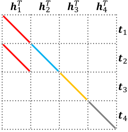
   (a) ogbl-biokg (AutoBLM)

   

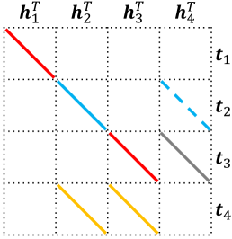
   (b) ogbl-wikikg2 (AutoBLM)

   

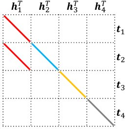
   (c) ogbl-biokg (AutoBLM+)

   

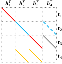
   (d) ogbl-wikikg2 (AutoBLM+)

   Figure 13: A graphical illustration of $g_{4}(\bm{A},\bm{r})$ identified by AutoBLM and AutoBLM+ on the large-scale KG completion task with ogbl-biokg and ogbl-wikikg2 datasets.

   

   

   

   

   

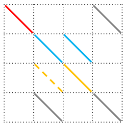
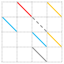
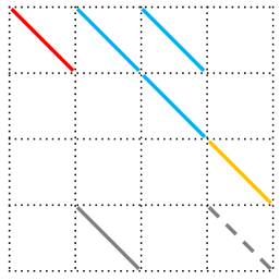
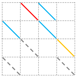
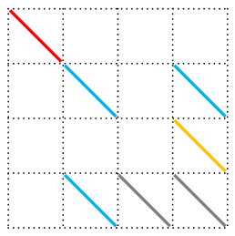
   (a) FB15k-2p.

   

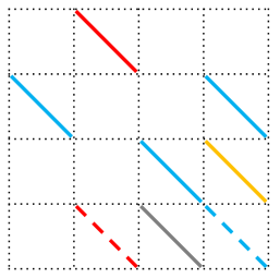
   (b) FB15k-3p.

   

   (c) FB15k237-2p.

   

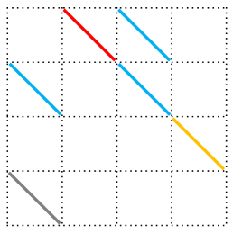
   (d) FB15k237-3p.

   Figure 14: A graphical illustration of $g_{4}(\bm{A},\bm{r})$ identified by AutoBLM (top) and AutoBLM+ (bottom) on the multi-hop query task.

   

   

   

   

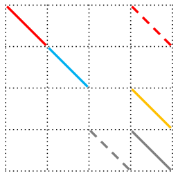
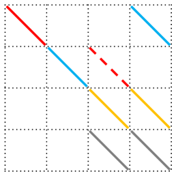
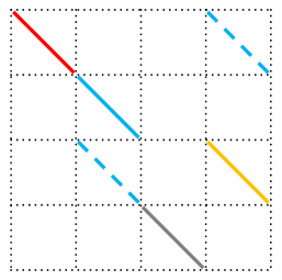
   (a) AIFB.

   

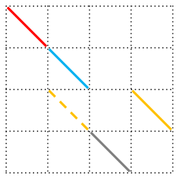
   (b) MUTAG.

   

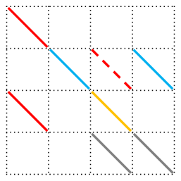
   (c) BGS.

   Figure 15: A graphical illustration of $g_{4}(\bm{A},\bm{r})$ identified by AutoBLM (top) and AutoBLM+ (bottom) on the entity classification task.

   $$f_{\bm{A}^{\prime}}(h,r,t)$$

   $$=\sum\nolimits_{i=1}^{K}\sum\nolimits_{j=1}^{K}\text{sign}(A^{\prime}_{ij})\langle\bm{h}^{\prime}_{i},\bm{r}^{\prime}_{|A^{\prime}_{ij}|},\bm{t}^{\prime}_{j}\rangle,$$

   $$=\sum\nolimits_{i=1}^{K}\sum\nolimits_{j=1}^{K}s_{|A_{ij}|}\cdot\text{sign}(A_{ij})\cdot\langle{\bm{h}}_{i}^{*},s_{|A_{ij}|}\cdot{\bm{r}}_{|A_{ij}|}^{*},{\bm{t}}_{j}^{*}\rangle,$$

   $$=\sum\nolimits_{i=1}^{K}\sum\nolimits_{j=1}^{K}s_{|A_{ij}|}^{2}\cdot\text{sign}(A_{ij})\cdot\langle{\bm{h}}_{i}^{*},{\bm{r}}_{|A_{ij}|}^{*},{\bm{t}}_{j}^{*}\rangle,$$

   $$=\sum\nolimits_{i=1}^{K}\sum\nolimits_{j=1}^{K}\text{sign}(A_{ij})\cdot\langle{\bm{h}}_{i}^{*},{\bm{r}}_{|A_{ij}|}^{*},{\bm{t}}_{j}^{*}\rangle,$$

   $$=f_{\bm{A}}(h,r,t),$$

   with $s_{|A_{ij}|}^{2}=1$.

   Similarly, given ${\bm{E}^{\prime}}^{*},{\bm{R}^{\prime}}^{*}$ as the optimal embeddings trained by $f_{\bm{A}^{\prime}}(h,r,t)$, we can set $\bm{E},\bm{R}$ with $\bm{E}={\bm{E}^{\prime}}^{*},\bm{R}_{k}=s_{k}\cdot{\bm{R}^{\prime}}_{k}^{*},k=1\dots K$. In this way, we always have

   $$f_{\bm{A}}(h,r,t)$$

   $$=\sum\nolimits_{i=1}^{K}\sum\nolimits_{j=1}^{K}\text{sign}(A_{ij})\langle\bm{h}_{i},\bm{r}_{|A_{ij}|},\bm{t}_{j}\rangle,$$

   $$=\sum\nolimits_{i=1}^{K}\sum\nolimits_{j=1}^{K}s_{|A^{\prime}_{ij}|}\cdot\text{sign}(A^{\prime}_{ij})\cdot\langle{\bm{h}^{\prime}}_{i}^{*},s_{|A^{\prime}_{ij}|}\cdot{\bm{r}^{\prime}}_{|A^{\prime}_{ij}|}^{*},{\bm{t}^{\prime}}_{j}^{*}\rangle,$$

   $$=\sum\nolimits_{i=1}^{K}\sum\nolimits_{j=1}^{K}s_{|A^{\prime}_{ij}|}^{2}\cdot\text{sign}(A^{\prime}_{ij})\cdot\langle{\bm{h}^{\prime}}_{i}^{*},{\bm{r}^{\prime}}_{|A^{\prime}_{ij}|}^{*},{\bm{t}^{\prime}}_{j}^{*}\rangle,$$

   $$=\sum\nolimits_{i=1}^{K}\sum\nolimits_{j=1}^{K}\text{sign}(A^{\prime}_{ij})\cdot\langle{\bm{h}^{\prime}}_{i}^{*},{\bm{r}^{\prime}}_{|A^{\prime}_{ij}|}^{*},{\bm{t}^{\prime}}_{j}^{*}\rangle,$$

   $$=f_{\bm{A}^{\prime}}(h,r,t).$$

   Finally, based on Lemma 10, we have $\bm{A}\equiv\bm{A}^{\prime}$.

∎

Appendix B Relation distribution in different datasets

Following [71], if more than half of the training triples of a relation $r$ have inverse triples (i.e., $|\{(t,r,h)\in\mathcal{S}_{\text{tra}}:(h,r,t)\in\mathcal{S}_{\text{tra}}\}|>\frac{1}{2}|\{(h,r,t)\in\mathcal{S}_{\text{tra}}\}|$), $r$ is considered as symmetric. If there exists no inverse triplet (i.e., $|\{(t,r,h)\in\mathcal{S}_{\text{tra}}:(h,r,t)\in\mathcal{S}_{\text{tra}}\}|=0$), $r$ is anti-symmetric. Relations that are neither symmetric nor anti-symmetric are general asymmetric. Finally, a relation $r$ belongs to the inverse type if $\exists r^{\prime}\in\mathcal{R}:|\{(t,r^{\prime},h)\in\mathcal{S}_{\text{tra}}:(h,r,t)\in\mathcal{S}_{\text{tra}}\}|>\frac{1}{2}|\{(h,r,t)\in\mathcal{S}_{\text{tra}}\}|$.

As can be seen, the four datasets have very different distributions and thus properties. As demonstrated in neural architecture search [32, 31, 30], different datasets need different neural architectures. The architectures discovered have better performance than those designed by humans. Hence, the scoring functions should also be data-dependent, as demonstrated empirically in Section 5.1.2.

TABLE XIII: Distribution of relation types in the testing set.

	symmetry	anti-symmetry	general asymmetry	inverse
WN18	23.4%	72.1%	4.5%	4.5%
FB15k	9.3%	5.2%	85.5%	74.9%
WN18RR	37.4%	59.0%	3.6%	0.0%
FB15k237	3.0%	8.5%	88.5%	10.5%
YAGO3-10	3.4%	0.7%	95.9%	8.2%

Appendix C Consistent performance under different dimensions

In this section, we perform the KG completion experiment in Section 5.1. First, we collect the first 100 structures $\bm{A}$’s (with $d=64$) of AutoBLM+ in Section 5.1 and measure the corresponding validation MRR performance in step 18 of Algorithm 4. We then increase the embedding dimensionality to $1024$, retrain and re-evaluate these structures. Figure 16 compares the validation MRRs obtained with $d=64$ and $d=1024$ on the WN18RR and FB15k-237 data sets. As can be seen, the two sets of MRRs are correlated, especially for the top performed ones. The Spearman’s rank correlation coefficient on WN18RR is $0.4255$ and on FB15k-237 is $0.7054$.

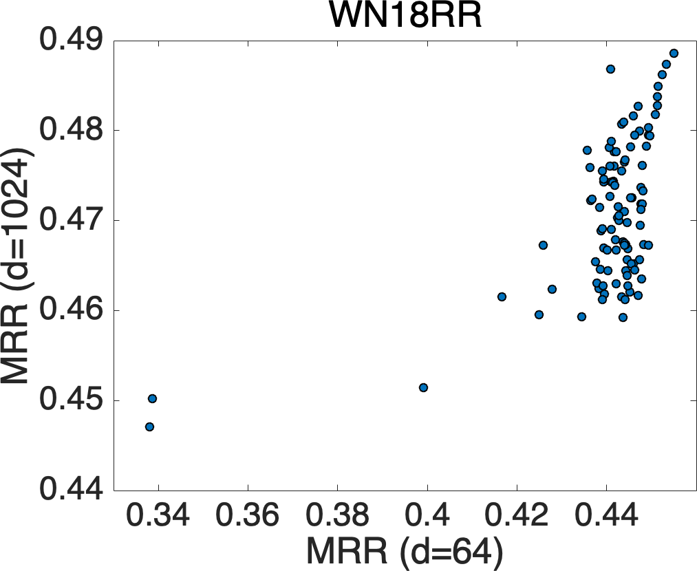
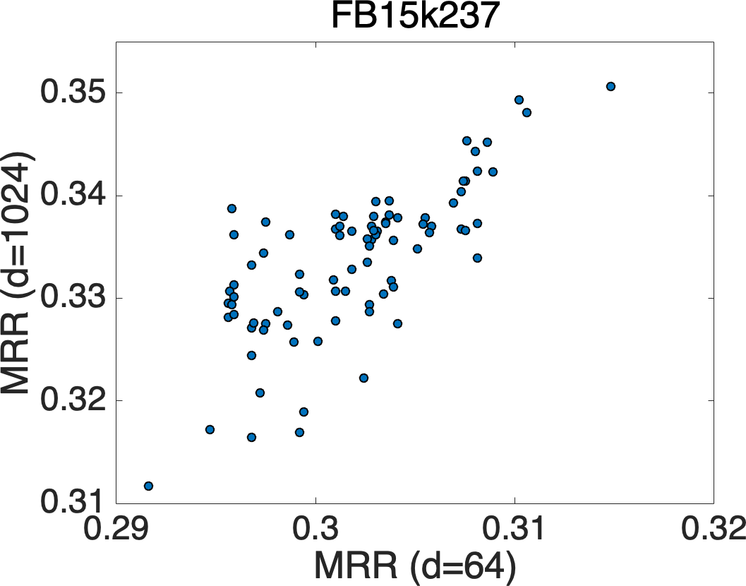
Figure 16: Validation MRRs of the structures with $d=64$ and $d=1024$.

Appendix D Models Obtained by AutoBLM and AutoBLM+

Figures 13, 14 and 15 show the structures obtained by AutoBLM and AutoBLM+ on the tasks of KG completion (Section 5.1) for the ogbl-biokg and ogbl-wikikg2 datasets, multi-hop query (Section 5.2) and entity classification (Section 5.3), respectively.

References

- [1] A. Singhal, “Introducing the knowledge graph: Things, not strings,” Official Google blog, vol. 5, 2012.
- [2] M. Nickel, K. Murphy, V. Tresp, and E. Gabrilovich, “A review of relational machine learning for knowledge graphs,” Proceedings of the IEEE, vol. 104, no. 1, pp. 11–33, 2016.
- [3] Q. Wang, Z. Mao, B. Wang, and L. Guo, “Knowledge graph embedding: A survey of approaches and applications,” TKDE, vol. 29, no. 12, pp. 2724–2743, 2017.
- [4] H. Ren, W. Hu, and J. Leskovec, “Query2box: Reasoning over knowledge graphs in vector space using box embeddings,” in ICLR, 2020.
- [5] F. Zhang, N. J. Yuan, D. Lian, X. Xie, and W.-Y. Ma, “Collaborative knowledge base embedding for recommender systems,” in SIGKDD, 2016, pp. 353–362.
- [6] M. Nickel, V. Tresp, and H. Kriegel, “A three-way model for collective learning on multi-relational data,” in ICML, vol. 11, 2011, pp. 809–816.
- [7] B. Yang, W. Yih, X. He, J. Gao, and L. Deng, “Embedding entities and relations for learning and inference in knowledge bases,” in ICLR, 2015.
- [8] W. Hamilton, P. Bajaj, M. Zitnik, D. Jurafsky, and J. Leskovec, “Embedding logical queries on knowledge graphs,” in NeurIPS, 2018, pp. 2026–2037.
- [9] T. N. Kipf and M. Welling, “Semi-supervised classification with graph convolutional networks,” in ICLR, 2017.
- [10] A. Bordes, N. Usunier, A. Garcia-Duran, J. Weston, and O. Yakhnenko, “Translating embeddings for modeling multi-relational data,” in NIPS, 2013, pp. 2787–2795.
- [11] Z. Wang, J. Zhang, J. Feng, and Z. Chen, “Knowledge graph embedding by translating on hyperplanes,” in AAAI, vol. 14, 2014, pp. 1112–1119.
- [12] M. Fan, Q. Zhou, E. Chang, and T. F. Zheng, “Transition-based knowledge graph embedding with relational mapping properties,” in PACLIC, 2014.
- [13] Z. Sun, Z. Deng, J. Nie, and J. Tang, “RotatE: Knowledge graph embedding by relational rotation in complex space,” in ICLR, 2019.
- [14] T. Trouillon, C. Dance, E. Gaussier, J. Welbl, S. Riedel, and G. Bouchard, “Knowledge graph completion via complex tensor factorization,” JMLR, vol. 18, no. 1, pp. 4735–4772, 2017.
- [15] M. Nickel, L. Rosasco, and T. Poggio, “Holographic embeddings of knowledge graphs,” in AAAI, 2016, pp. 1955–1961.
- [16] H. Liu, Y. Wu, and Y. Yang, “Analogical inference for multi-relational embeddings,” in ICML, 2017, pp. 2168–2178.
- [17] M. Kazemi and D. Poole, “SimplE embedding for link prediction in knowledge graphs,” in NeurIPS, 2018.
- [18] T. Lacroix, N. Usunier, and G. Obozinski, “Canonical tensor decomposition for knowledge base completion,” in ICML, 2018.
- [19] S. Zhang, Y. Tay, L. Yao, and Q. Liu, “Quaternion knowledge graph embedding,” in NeurIPS, 2019.
- [20] X. Dong, E. Gabrilovich, G. Heitz, W. Horn, N. Lao, K. Murphy, T. Strohmann, S. Sun, and W. Zhang, “Knowledge vault: A web-scale approach to probabilistic knowledge fusion,” in SIGKDD, 2014, pp. 601–610.
- [21] T. Dettmers, P. Minervini, P. Stenetorp, and S. Riedel, “Convolutional 2D knowledge graph embeddings,” in AAAI, 2017.
- [22] L. Guo, Z. Sun, and W. Hu, “Learning to exploit long-term relational dependencies in knowledge graphs,” in ICML, 2019, pp. 2505–2514.
- [23] M. Schlichtkrull, T. N. Kipf, P. Bloem, R. Van Den Berg, I. Titov, and M. Welling, “Modeling relational data with graph convolutional networks,” in ESWC. Springer, 2018, pp. 593–607.
- [24] S. Vashishth, S. Sanyal, V. Nitin, and P. Talukdar, “Composition-based multi-relational graph convolutional networks,” in ICLR, 2020.
- [25] Y. Lin, X. Han, R. Xie, Z. Liu, and M. Sun, “Knowledge representation learning: A quantitative review,” arXiv:1812.10901, Tech. Rep., 2018.
- [26] Y. Wang, D. Ruffinelli, S. Broscheit, and R. Gemulla, “On evaluating embedding models for knowledge base completion,” RepL4NLP@ACL, Tech. Rep., 2018.
- [27] Q. Yao and M. Wang, “Taking human out of learning applications: A survey on automated machine learning,” arXiv: 1810.13306, Tech. Rep., 2018.
- [28] F. Hutter, L. Kotthoff, and J. Vanschoren, Eds., Automated machine learning: Methods, systems, challenges. Springer, 2018.
- [29] M. Feurer, A. Klein, K. Eggensperger, J. Springenberg, M. Blum, and F. Hutter, “Efficient and robust automated machine learning,” in NIPS, 2015, pp. 2962–2970.
- [30] B. Zoph and Q. Le, “Neural architecture search with reinforcement learning,” in ICLR, 2017.
- [31] H. Liu, K. Simonyan, and Y. Yang, “DARTS: Differentiable architecture search,” in ICLR, 2019.
- [32] T. Elsken, J. H. Metzen, and F. Hutter, “Neural architecture search: A survey,” JMLR, vol. 20, no. 55, pp. 1–21, 2019.
- [33] Y. Zhang, Q. Yao, W. Dai, and L. Chen, “AutoSF: Searching scoring functions for knowledge graph embedding,” in ICDE, 2020, pp. 433–444.
- [34] Y. Wang, R. Gemulla, and H. Li, “On multi-relational link prediction with bilinear models,” in AAAI, 2017.
- [35] I. Balažević, C. Allen, and T. M. Hospedales, “Tucker: Tensor factorization for knowledge graph completion,” in EMNLP, 2019.
- [36] S. Ji, S. Pan, E. Cambria, P. Marttinen, and P. S. Yu, “A survey on knowledge graphs: Representation, acquisition and applications,” TNNLS, 2021.
- [37] Y. Bengio, A. Courville, and P. Vincent, “Representation learning: A review and new perspectives,” TPAMI, vol. 35, no. 8, pp. 1798–1828, 2013.
- [38] R. Socher, D. Chen, C. Manning, and A. Ng, “Reasoning with neural tensor networks for knowledge base completion,” in NIPS, 2013, pp. 926–934.
- [39] K. Guu, J. Miller, and P. Liang, “Traversing knowledge graphs in vector space,” in EMNLP, 2015, pp. 318–327.
- [40] Y. Zhang, Q. Yao, and L. Chen, “Interstellar: Searching recurrent architecture for knowledge graph embedding,” NeurIPS, vol. 33, pp. 10 030–10 040, 2020.
- [41] S. Hochreiter and J. Schmidhuber, “Long short-term memory,” Neural Computation, vol. 9, no. 8, pp. 1735–1780, 1997.
- [42] K. Hayashi and M. Shimbo, “On the equivalence of holographic and complex embeddings for link prediction,” in ACL, vol. 2, 2017, pp. 554–559.
- [43] L. R. Tucker, “Some mathematical notes on three-mode factor analysis,” Psychometrika, vol. 31, no. 3, pp. 279–311, 1966.
- [44] J. Gilmer, S. S. Schoenholz, P. F. Riley, R. Vinyals, and G. E. Dahl, “Neural message passing for quantum chemistry,” in ICML, 2017, pp. 1263–1272.
- [45] B. Colson, P. Marcotte, and G. Savard, “An overview of bilevel optimization,” Annals of Operations Research, vol. 153, no. 1, pp. 235–256, 2007.
- [46] G. Bender, P. Kindermans, B. Zoph, V. Vasudevan, and Q. Le, “Understanding and simplifying one-shot architecture search,” in ICML, 2018, pp. 549–558.
- [47] H. Pham, M. Guan, B. Zoph, Q. Le, and J. Dean, “Efficient neural architecture search via parameters sharing,” in ICML, 2018, pp. 4095–4104.
- [48] Q. Yao, J. Xu, W. Tu, and Z. Zhu, “Efficient neural architecture search via proximal iterations,” in AAAI, 2020.
- [49] C. Liu, B. Zoph, S. Jonathon, W. Hua, L. Li, F.-F. Li, A. Yuille, J. Huang, and K. Murphy, “Progressive neural architecture search,” in ECCV, 2018.
- [50] E. Real, A. Aggarwal, Y. Huang, and Q. V. Le, “Regularized evolution for image classifier architecture search,” in AAAI, vol. 33, 2019, pp. 4780–4789.
- [51] J. A. Tropp, “Greed is good: Algorithmic results for sparse approximation,” TIT, vol. 50, no. 10, pp. 2231–2242, 2004.
- [52] T. Back, Evolutionary algorithms in theory and practice: evolution strategies, evolutionary programming, genetic algorithms. Oxford university press, 1996.
- [53] A. Paszke, S. Gross, S. Chintala, G. Chanan, E. Yang, Z. DeVito, Z. Lin, A. Desmaison, L. Antiga, and A. Lerer, “Automatic differentiation in PyTorch,” in ICLR, 2017.
- [54] G. A. Miller, “WordNet: A lexical database for english,” Communications of the ACM, vol. 38, no. 11, pp. 39–41, 1995.
- [55] K. Bollacker, C. Evans, P. Paritosh, T. Sturge, and J. Taylor, “Freebase: A collaboratively created graph database for structuring human knowledge,” in SIGMOD, 2008, pp. 1247–1250.
- [56] K. Toutanova and D. Chen, “Observed versus latent features for knowledge base and text inference,” in Workshop on CVSMC, 2015, pp. 57–66.
- [57] F. Suchanek, G. Kasneci, and G. Weikum, “Yago: A core of semantic knowledge,” in WWW, 2007, pp. 697–706.
- [58] W. Hu, M. Fey, M. Zitnik, Y. Dong, H. Ren, B. Liu, M. Catasta, and J. Leskovec, “Open graph benchmark: Datasets for machine learning on graphs,” NeurIPS, vol. 33, pp. 22 118–22 133, 2020.
- [59] D. Vrandečić and M. Krötzsch, “Wikidata: a free collaborative knowledgebase,” Communications of the ACM, vol. 57, no. 10, pp. 78–85, 2014.
- [60] F. Mahdisoltani, J. Biega, and F. M. Suchanek, “Yago3: A knowledge base from multilingual wikipedias,” in CIDR, 2013.
- [61] L. Chao, J. He, T. Wang, and W. Chu, “Pairre: Knowledge graph embeddings via paired relation vectors,” in ACL, 2021, pp. 4360–4369.
- [62] X. Kou, B. Luo, H. Hu, and Y. Zhang, “Nase: Learning knowledge graph embedding for link prediction via neural architecture search,” in ICIKM, 2020, pp. 2089–2092.
- [63] Y. Wang, D. Ruffinelli, R. Gemulla, S. Broscheit, and C. Meilicke, “On evaluating embedding models for knowledge base completion,” in RepL4NLP-2019, 2019, pp. 104–112.
- [64] P. Tabacof and L. Costabello, “Probability calibration for knowledge graph embedding models,” in ICLR, 2019.
- [65] J. Duchi, E. Hazan, and Y. Singer, “Adaptive subgradient methods for online learning and stochastic optimization,” JMLR, vol. 12, no. Jul, pp. 2121–2159, 2011.
- [66] J. S. Bergstra, R. Bardenet, Y. Bengio, and B. Kégl, “Algorithms for hyper-parameter optimization,” in NIPS, 2011, pp. 2546–2554.
- [67] R. J. Williams, “Simple statistical gradient-following algorithms for connectionist reinforcement learning,” Machine Learning Journal, vol. 8, no. 3-4, pp. 229–256, 1992.
- [68] P. Ristoski and H. Paulheim, “Rdf2vec: Rdf graph embeddings for data mining,” in ISWC. Springer, 2016, pp. 498–514.
- [69] D. P. Kingma and J. Ba, “Adam: A method for stochastic optimization,” in ICLR, 2015.
- [70] R. A. Horn and C. R. Johnson, Matrix analysis. Cambridge university press, 2012.
- [71] A. Rossi, D. Firmani, A. Matinata, P. Merialdo, and D. Barbosa, “Knowledge graph embedding for link prediction: A comparative analysis,” TKDD, 2021.