Root and community inference on the latent growth process of a network

Abstract

Many existing statistical models for networks overlook the fact that most real world networks are formed through a growth process. To address this, we introduce the PAPER (Preferential Attachment Plus Erdős–Rényi) model for random networks, where we let a random network G be the union of a preferential attachment (PA) tree T and additional Erdős–Rényi (ER) random edges. The PA tree component captures the underlying growth/recruitment process of a network where vertices and edges are added sequentially, while the ER component can be regarded as random noise. Given only a single snapshot of the final network G, we study the problem of constructing confidence sets for the early history, in particular the root node, of the unobserved growth process; the root node can be patient zero in a disease infection network or the source of fake news in a social media network. We propose an inference algorithm based on Gibbs sampling that scales to networks with millions of nodes and provide theoretical analysis showing that the expected size of the confidence set is small so long as the noise level of the ER edges is not too large. We also propose variations of the model in which multiple growth processes occur simultaneously, reflecting the growth of multiple communities, and we use these models to provide a new approach to community detection.

1 Introduction

Network data is ubiquitous. To analyze networks, there are a variety of statistical models such as Erdős–Rényi, stochastic block model (SBM) (Abbe, 2017; Karrer and Newman, 2011; Amini et al., 2013; Xu et al., 2018), graphon (Diaconis and Janson, 2007; Gao et al., 2015), random dot product graphs (Athreya et al., 2017; Xie and Xu, 2019), latent space models (Hoff et al., 2002), configuration graphs (Aiello et al., 2000), and more. These models usually operate by specifying some structure, such as community structure in the case of SBM, and then adding independent random edges in a way that reflects the structure. The order in which the edges are added is of no importance to these models.

In contrast, real world networks are often formed from growth processes where vertices and edges are added sequentially. This motivates the development of Markovian preferential attachment (PA) models for networks (Barabási and Albert, 1999; Barabási, 2016) which produce a sequence of networks $\bm{G}_{1},\bm{G}_{2},\ldots,\bm{G}_{n}$ where $\bm{G}_{1}$ starts as a single node which we call the root node and, at each iteration, we add a new node and new edges. PA models naturally produce networks with sparse edges, heavy-tailed degree distributions, and strands of chains as well as pendants (several degree 1 vertices linked to a single vertex), which are important features of real world networks that are difficult to reproduce under a non-Markovian model, as observed by Bloem-Reddy and Orbanz (2018).

Although Markovian models are often more realistic, they have not been as widely used in network data analysis as, say SBM, because, whereas SBM is useful for recovering the community structure of a network, it is not obvious what structural information Markovian models could extract from a network. Recently however, seminal work from a series of applied probability papers (e.g. Bubeck, Devroye and Lugosi (2017); Bubeck et al. (2015)) demonstrate that Markovian models can indeed recover useful structure: these papers show that, surprisingly, when $\bm{G}_{n}$ is a random PA tree, one can infer the early history of $\bm{G}_{n}$, such as the root node, even as the size of the tree tends to infinity. Although these results are elegant, they are theoretical; their confidence set construction involves large constants that render the result too conservative. Moreover, most algorithms apply only to tree-shaped networks, which prohibitively limits their application since trees are rarely encountered in practice.

To overcome these problems, we propose a Markovian model for networks which we call Preferential Attachment Plus Erdős–Rényi, or PAPER for short. We say that $\bm{G}_{n}$ has the PAPER distribution if it is generated by adding independent random edges to a preferential attachment tree $\bm{T}$. The latent PA tree captures the growth process of the network whereas the ER random edges can be interpreted as additional noise. Given only a single snapshot of the final graph $\bm{G}_{n}$, we study how to infer the early history of the latent tree $\bm{T}$, focusing on the concrete problem of constructing confidence sets for the root node that can attain the nominal coverage. We give a visual illustration of the PAPER model and the inference problem in Figure 1.

Because we do not know which edges of $\bm{G}_{n}$ correspond to the tree and which are noise, most existing methods are not directly applicable. We therefore propose a new approach in which we first give the nodes new random labels which induce, for a given observation of the network $\bm{G}_{n}$, a posterior distribution of both the latent tree and the latent arrival ordering of the nodes. Then, we sample from the posterior distribution to construct a credible set for the inferential target, e.g. the root node. Bayesian inference statements usually do not have frequentist validity but we prove in our setting that that the level $1-\epsilon$ credible set for the root node has frequentist coverage at exactly the same level.

In order to efficiently sample from the posterior distribution of the latent ordering and the latent tree, we present a scalable Gibbs sampler that alternatingly samples the ordering and the tree. The algorithm to generate the latent ordering is based on our previous work (Crane and Xu, 2021) which studies inference in the tree setting. The algorithm to generate the latent tree operates by updating the parent of each of the nodes iteratively. The overall runtime complexity of one iteration of the outer loop is generally $O(m+n\log n)$ (where $m$ is the number of edges) and the algorithm can scale to networks of up to a million nodes.

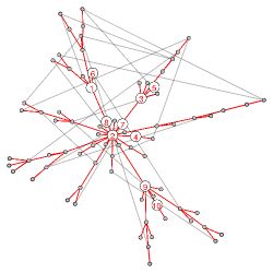
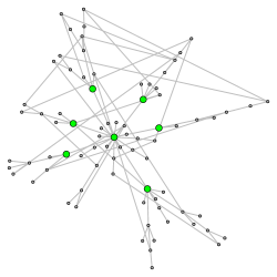
Figure 1: Left: illustration of PAPER model; nodes have latent time ordering (only first 10 orderings shown); the red edges form the latent tree while gray edges are Erdős–Rényi. Right: 80% confidence set for the root node (node number 1) constructed from the unlabeled graph.

Since a trivial confidence set for the root node is the set of all the nodes, it is important to be able to bound the size of a confidence set. In particular, the presence of noisy Erdős–Rényi edges in the PAPER model motivates an interesting question: how does the size of the confidence set increase with the noise level? In this paper, we give an initial answer to this question under two specific settings of the preferential attachment mechanism: linear preferential attachment (LPA) and uniform attachment (UA). For LPA, we prove that the size of our proposed confidence set does not increase with the number of nodes $n$ so long as the noisy edge probability is less than $n^{-1/2}$ and for UA, we prove that the size is bounded by $n^{\gamma}$ for some $\gamma<1$ so long as the noisy edge probability is less than $\log(n)/n$. Our analysis shows that the phenomenon discovered by Bubeck, Devroye and Lugosi (2017), that there exists confidence sets for the root node of $O(1)$ size, is robust to the presence of noise.

Many real world networks often have community structures. In such cases, it would be unrealistic to assume that the network originates from a single root node. We therefore propose variations of the PAPER model in which $K$ growth processes occur simultaneously from $K$ root nodes. Each of $K$ root nodes can be interpreted as being locally central with respect to a community subgraph. In the multiple roots model, there is no longer a latent tree but rather a latent forest (union of disjoint trees), where the components of the forest can naturally be interpreted as the different communities of the network. We provide model formulation that allows $K$ to be either be fixed or random. To analyze networks with multiple roots, we use essentially the same inferential approach and Gibbs sampling algorithm that that we develop for the single root setting, with minimal modifications.

By looking at the posterior probability that a node is in a particular tree–community, we can estimate the community membership of each of the nodes. Compared with say the stochastic block model, the PAPER model approach to community recovery has the advantage that the inference quality improves with sparsity, that we can handle heavy-tailed degree distribution without a high-dimensional degree correction parameter vector, and that the posterior root probabilities also identify the important nodes in the community. Empirically, we show that our approach has competitive performance on two benchmark datasets and we find that our community membership estimate is more accurate for nodes with high posterior root probability than for the more peripheral nodes. We also use the PAPER model to conduct an extensive analysis of a statistician co-authorship network curated by Ji and Jin (2016) where we recover a large number of communities that accurately reflect actual research communities in statistics.

We have implemented our inference algorithm in a Python package called paper-network, which can be installed via command pip install paper-network. The code, example scripts, and documentation are all publicly available at https://github.com/nineisprime/PAPER.

Outline for the paper: In Section 2, we define the PAPER model in both the single root and multiple roots setting. We also formalize the problem of root inference and review related work. In Section 3, we describe our approach to the root inference problem, which is to randomize the node labels and analyze the resulting posterior distribution. We also show that the Bayesian inferential statements have frequentist validity. In Section 4, we give a sampling algorithm for computing the posterior probabilities. In Section 5, we provide theoretical bounds on the size of our proposed confidence sets and in Section 6, we provide empirical study on both simulated and large scale real world networks.

1.1 Notation

• We take all graphs to be undirected. Given two labeled graphs $\bm{g}$ and $\bm{g}^{\prime}$ defined on the same set of nodes, we write $\bm{g}+\bm{g}^{\prime}$ as the resulting graph if we take the union of the edges in $\bm{g}$ and $\bm{g}^{\prime}$ and collapse any multi-edges. We also write $\bm{g}\subset\bm{g}^{\prime}$ if $\bm{g}$ is a subgraph of $\bm{g}^{\prime}$.

• For a labeled graph $\bm{g}$, we write $D_{\bm{g}}(u)$ as the degree of node $u$ in graph $\bm{g}$ and $N_{\bm{g}}(u)$ as the set of neighbors of $u$ (all nodes directly connected to $u$) with respect to $\bm{g}$; we write $V(\bm{g})$ and $E(\bm{g})$ as the set of vertices and edges of $\bm{g}$ respectively.

• For an integer $n$, we write $[n]:=\{1,2,\ldots,n\}$ and for a discrete set $A$, we write $|A|$ as the cardinality of $A$. For two countable sets $A,B$ of the same cardinality, we write $\text{Bi}(A,B)$ as the set of bijections between them. For a vector $\pi$, we write $\pi_{1:K}$ to denote the sub-vector $(\pi_{1},\pi_{2},\ldots,\pi_{K})$.

• Given a finite set $V^{\prime}$ of the same cardinality of $V(\bm{g})$ and given a bijection $\rho\in\text{Bi}(V(\bm{g}),V^{\prime})$, we write $\rho\bm{g}$ to denote a relabeled graph where a pair $(u^{\prime},v^{\prime})\in V^{\prime}\times V^{\prime}$ is an edge in $\rho\bm{g}$ if and only if $(u,v)\in V(\bm{g})\times V(\bm{g})$ is an edge in $\bm{g}$.

• Throughout the paper, we use capital font (e.g. $\bm{G}$) to denote random objects and lower case font to denote fixed objects. Graphs are represented via bold font.

2 Model and Problem

We first describe the model and inference problem in the single root setting and then extend the definition to the setting of having fixed $K$ roots and having random $K$ roots.

2.1 PAPER model

Definition 1.

The affine preferential attachment tree model, which we denote by $\text{APA}(\alpha,\beta)$ for parameters $\alpha,\beta\in\mathbb{R}$, generates an increasing sequence $\bm{T}_{1}\subset\bm{T}_{2}\subset\ldots\subset\bm{T}_{n}$ of random trees where $\bm{T}_{t}$ is a tree with $t$ nodes and where nodes are labeled by their arrival time so that $V(\bm{T}_{t})=[t]$. The first tree $\bm{T}_{1}=\{1\}$ is a singleton and for $t>2$, we define the transition kernel $\mathbb{P}(\bm{T}_{t}\,|\,\bm{T}_{t-1})$ in the following way: given $\bm{T}_{t-1}$, we add a node labeled $t$ and a random edge $(t,w_{t})$ to obtain $\bm{T}_{t}$, where the existing node $w_{t}\in[t-1]$ is chosen with probability

$$\frac{\beta D_{\bm{T}_{t-1}}(w_{t})+\alpha}{\beta 2(t-2)+\alpha(t-1)}.$$ (1)

We may verify that (1) describes a valid probability distribution by noting that $\bm{T}_{t-1}$ always has $t-2$ edges and $t-1$ nodes. Before continuing onto the PAPER model, we consider some specific examples of APA trees:

1. setting $\alpha=1,\beta=0$ means that we select $w_{t}$ uniformly at random from $V(\bm{T}_{t-1})$. This yields the uniform attachment (UA) random tree. The resulting degree distribution has exponential tail and the maximum degree is of order $\log n$ (Na and Rapoport, 1970; Addario-Berry and Eslava, 2018).

2. Setting $\alpha=0,\beta=1$ means that we select $w_{t}$ with probability proportional to the degree $D_{\bm{T}_{k-1}}(w_{t})$. This yields the linear preferential attachment random (LPA) tree. LPA has heavy-tailed degree distribution and a maximum degree is of order $\sqrt{n}$ (Bollobás et al., 2001; Peköz et al., 2014).

3. We may also set $\beta$ as $-1$ and $\alpha$ as some positive integer so that the maximum degree of any node is $\alpha$. This may be interpreted as an uniform attachment tree growing on top of a background infinite $\alpha$-regular tree (Khim and Loh, 2017).

We may generalize Definition 1 by defining a nonparametric function $\phi\,:\,\mathbb{N}\rightarrow[0,\infty)$ and choose $w_{t}$ with probability proportional to $\phi(D_{\bm{T}_{t-1}}(w_{t}))$. In this paper however, we focus only on the case where $\phi$ is an affine function.

Definition 2.

To model a general network, we define the $\text{PAPER}(\alpha,\beta,\theta)$ (Preferential Attachment Plus Erdős–Rényi) model parametrized by $\alpha,\beta\in\mathbb{R}$ and $\theta\in[0,1]$. We say that a random graph $\bm{G}_{n}$ distributed according to the $\text{PAPER}(\alpha,\beta,\theta)$ model if

$$\bm{G}_{n}=\bm{T}_{n}+\bm{R}_{n},$$

where $\bm{T}_{n}\sim\text{APA}(\alpha,\beta)$ and $\bm{R}_{n}\sim\text{Erd\H{o}s--R\'{e}nyi}(\theta)$ are independent random graphs defined on the same set of vertices $[n]$.

Since we collapse any multi-edges that occur when we add $\bm{R}_{n}$ to $\bm{T}_{n}$, we may view $\bm{R}_{n}$ equivalently as an ER random graph defined on potential edges excluding those already in the tree $\bm{T}_{n}$. The PAPER model can produce networks with either light tailed or heavy tailed degree distribution depending on the choice of the parameters $\alpha$ and $\beta$. It produces features that are commonly seen in real world networks but absent from non-sequential models like SBM, such as pendants (a node with several degree-1 node attached to it) and chains of nodes; see Figure 2. It also assigns a non-zero probability to any connected graph, in contrast to the general preferential attachment graph model where a fixed $m>1$ edges are added at every iteration (Barabási and Albert, 1999). In computer science terminology, $\bm{G}_{n}$ is a planted tree model where the signal $\bm{T}_{n}$ is planted in an ER random graph $\bm{R}_{n}$ in the same sense that stochastic block model is often referred to as the planted partition model.

An alternative way to define the PAPER model is to specify the total number of edges $m$ in the final graph and generate $\bm{R}_{n}$ as a uniformly random graph with $m-(n-1)$ edges (since a tree with $n$ nodes always has $n-1$ edges). This is equivalent to the $\text{PAPER}(\alpha,\beta,\theta)$ model where we condition on the event that the final graph $\bm{G}_{n}$ has $m$ edges. To simplify exposition, we use PAPER to refer to this conditional model as well.

Remark 1.

We may view the $\text{PAPER}(\alpha,\beta,\theta)$ model as a Markovian process over a sequence of networks $\bm{G}_{1},\bm{G}_{2},\ldots,\bm{G}_{n}$. We define the transition kernel $\mathbb{P}(\bm{G}_{t}\,|\,\bm{G}_{t-1})$ for $t\geq 3$ by first adding a new node labeled $t$, then adding a new tree edge $(t,w_{t})$ where $w_{t}$ is chosen with probability (1), and then, for each existing node $j\in[t-1]$ not equal to $w_{t}$, we independently add a noise edge $(t,j)$ with probability $\theta$. In Section 2.3, we extend the PAPER model so that the noise edge probability depends on time $t$ and the state of the tree at time $t$.

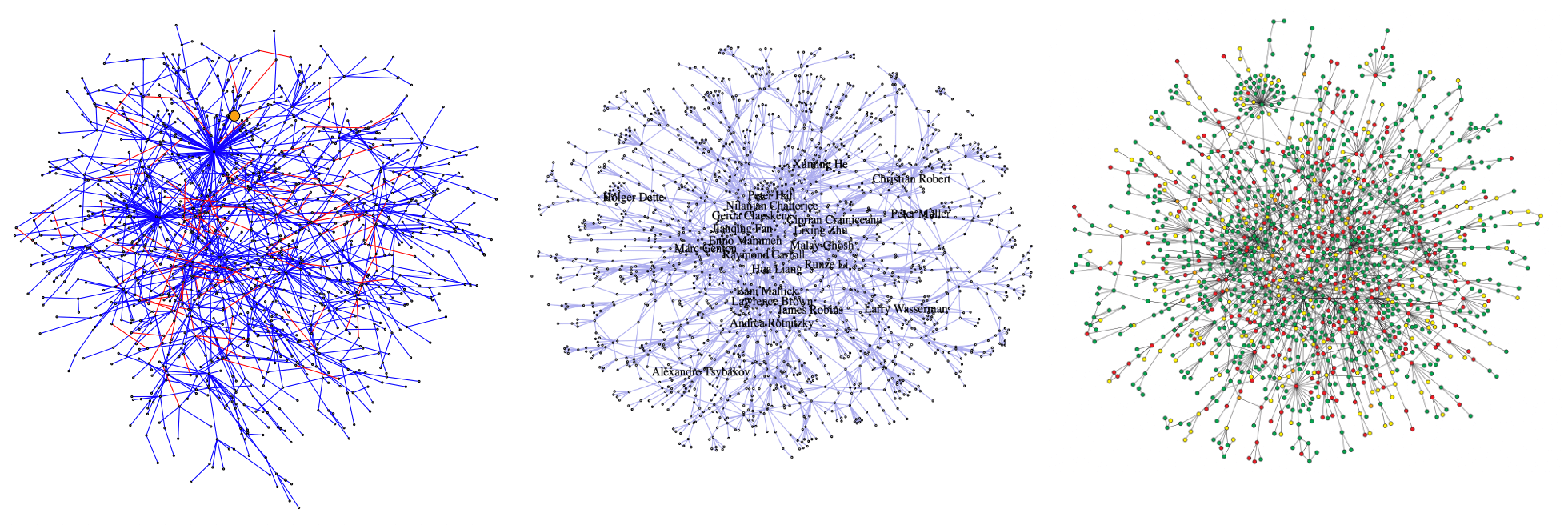
Figure 2: Left: PAPER graph with $\alpha=1,\beta=1$; Center: co-authorship graph from Ji and Jin (2016); Right: protein-protein interaction graph from Jeong et al. (2001).

Remark 2.

Under $\text{APA}(\alpha,\beta)$ model, the probability of generating a given tree has a closed form expression: $\mathbb{P}(\bm{T}_{n}=\bm{t}_{n})=\frac{\prod_{v\in[n]}\prod_{j=1}^{D_{\bm{t}_{n}}(v)-1}(\beta j+\alpha)}{\prod_{t=3}^{n}2(t-2)\beta+(t-1)\alpha}$. The important consequence is that the likelihood depends on the tree $\bm{t}_{n}$ only through its degree distribution $D_{\bm{t}_{n}}(\cdot)$. Hence, any two trees with the same degree distribution has the same likelihood; Crane and Xu (2021) refers to this property as shape-exchangeability. We give the likelihood expression for the multiple roots models and the PAPER model in Section S1.1 of the Appendix.

Remark 3.

In many settings, it is known that the degree distribution of an $\text{APA}(\alpha,\beta)$ tree has an asymptotic limit. For example, if $\beta=1$ and $\alpha>0$, then we have by Van Der Hofstad (2016, Theorem 8.2) that $\frac{1}{n}\sum_{t=1}^{n}\mathbbm{1}\{D_{\bm{T}_{n}}(t)=k\}\rightarrow\frac{2+\alpha}{3+2\alpha}\prod_{j=1}^{k-1}\frac{j+\alpha}{j+3+2\alpha}$ as $n\rightarrow\infty$ uniformly over all $k$. The limiting distribution is approximately a power law where the number of nodes with degree $k$ is proportional to $k^{-(3+\alpha)}$ (see Van Der Hofstad (2016, Section 8.4)). Since the ER graph $\bm{R}_{n}$ only adds an expected additional degree of at most $n\theta$ to every node, we see that, when $\theta$ is small, the PAPER graph can have heavy-tailed degree distribution without any additional degree correction parameters.

Single root inference problem: Let $\bm{G}_{n}\sim\text{PAPER}(\alpha,\beta,\theta)$ be a random graph. Since the nodes of $\bm{G}_{n}$ are labeled by their arrival time, we observe only the unlabeled shape of $\bm{G}_{n}$. Equivalently, we may take our observation to be a labeled graph $\bm{G}^{*}_{n}$ whose nodes are labeled by an arbitrary alphabet $\mathcal{U}_{n}$ of $n$ elements, i.e., $V(\bm{G}^{*}_{n})=\mathcal{U}_{n}$. Then, there exists a label bijection $\rho\in\text{Bi}([n],\mathcal{U}_{n})$ such that $\rho\bm{G}_{n}=\bm{G}^{*}_{n}$.

The unobserved label bijection $\rho$ captures precisely the arrival time of the nodes in that for any $t\in[n]$, the node with label $\rho_{t}$ in $\bm{G}^{*}_{n}$ correspond precisely to node $t$ in $\bm{G}_{n}$. Therefore, we call any label bijection in $\text{Bi}([n],\mathcal{U}_{n})$ an ordering of the nodes.

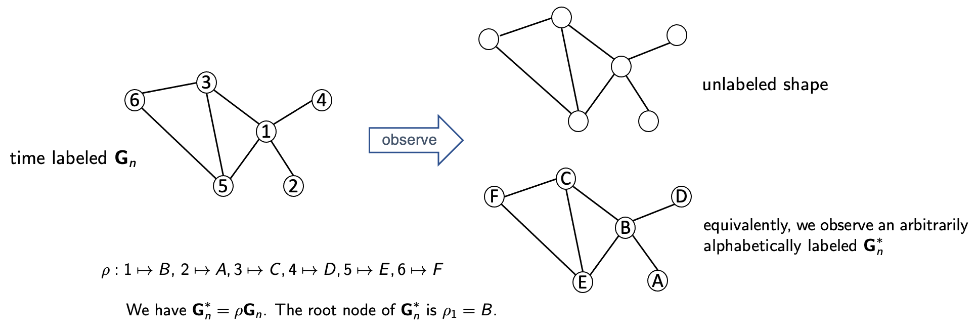
Figure 3: Our observation is the unlabeled shape or alphabetically labeled $\bm{G}^{*}_{n}$ instead of time labeled $\bm{G}_{n}$. There exists an unobserved ordering $\rho\in\text{Bi}([n],\mathcal{U}_{n})$ such that $\bm{G}^{*}_{n}=\rho\bm{G}_{n}$.

Our goal is to infer various aspects of the latent ordering $\rho$. We focus on the simpliest example of root inference. Since the node labeled 1 is the root node in $\bm{G}_{n}$, it corresponds to the node labeled $\rho_{1}$ in $\bm{G}^{*}_{n}$. Therefore, the node $\rho_{1}\in\mathcal{U}_{n}$ is the root node, that is, the first node in the growth process. To illustrate the setting clearly, we provide a specfic example in Figure 3.

Definition 3.

For $\epsilon\in(0,1)$, we say that a set $C_{\epsilon}(\bm{G}_{n}^{*})\subset\mathcal{U}_{n}$ is a level $1-\epsilon$ confidence set for the root node if

$$\mathbb{P}\bigl{(}\rho_{1}\in C_{\epsilon}(\bm{G}_{n}^{*})\bigr{)}\geq 1-\epsilon.$$ (2)

One may construct a trivial confidence set for the root nodes by taking the set of all the nodes. We aim therefore to make the confidence set $C_{\epsilon}(\cdot)$ as small as possible. Although we focus on the problem of root inference, the approach that we develop is applicable to more general problems such as inferring the first two or three nodes or inferring the arrival time of a particular node.

Remark 4.

It is important to note that $\bm{G}^{*}_{n}$ may have multiple nodes that are indistinguishable once the node labels are removed, which may lead to the paradoxical scenario that which node of $\bm{G}^{*}_{n}$ correspond to the true root node depends on the choice of the label bijection $\rho$. Luckily, this is a technical issue that does not pose a problem so long as we restrict ourselves to confidence sets $C_{\epsilon}(\cdot)$ that are labeling equivariant in that they do not depend on the specific node labeling. Labeling equivariance is a very weak condition that only rules out confidence sets that can access side information about the nodes somehow.

Formally, we note that there may exist $\rho,\rho^{\prime}\in\text{Bi}([n],\mathcal{U}_{n})$ where $\rho_{1}\neq\rho^{\prime}_{1}$ but both satisfy $\bm{G}^{*}_{n}=\rho\bm{G}_{n}=\rho^{\prime}\bm{G}_{n}$; in other words, root node can only be well-defined up to an automorphism. We illustrate a concrete example in Figure 4. We define $C_{\epsilon}(\cdot)$ to be labeling equivariant if, for all $\tau\in\text{Bi}(\mathcal{U}_{n},\mathcal{U}_{n})$, we have $\tau C_{\epsilon}(\bm{G}^{*}_{n})=C_{\epsilon}(\tau\bm{G}^{*}_{n})$; if the confidence set algorithm contains randomization (to break ties for example), then we say it is labeling equivariant if $\tau C_{\epsilon}(\bm{G}^{*}_{n})\stackrel{{\scriptstyle d}}{{=}}C_{\epsilon}(\tau\bm{G}^{*}_{n})$ for all $\tau\in\text{Bi}(\mathcal{U}_{n},\mathcal{U}_{n})$. If a confidence set $C_{\epsilon}(\cdot)$ is labeling equivariant, then for any $\rho,\rho^{\prime}\in\text{Bi}([n],\mathcal{U}_{n})$ such that $\bm{G}^{*}_{n}=\rho\bm{G}_{n}=\rho^{\prime}\bm{G}_{n}$, we have that $(\rho^{\prime}\circ\rho^{-1})\bm{G}^{*}_{n}=\bm{G}^{*}_{n}$ and hence,

$$\rho_{1}\in C_{\epsilon}(\bm{G}^{*}_{n})\Leftrightarrow(\rho^{\prime}\circ\rho^{-1})\rho_{1}\in(\rho^{\prime}\circ\rho^{-1})C_{\epsilon}(\bm{G}^{*}_{n})\Leftrightarrow\rho^{\prime}_{1}\in C_{\epsilon}((\rho^{\prime}\circ\rho^{-1})\bm{G}^{*}_{n})\Leftrightarrow\rho^{\prime}_{1}\in C_{\epsilon}(\bm{G}^{*}_{n}).$$

Therefore, the coverage probability (2) does not depend on the choice of $\rho$.

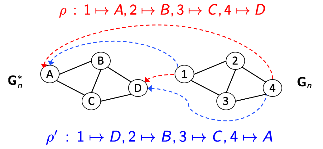
Figure 4: Both $\rho$ (red) and $\rho^{\prime}$ (blue) are distinct bijections in $\text{Bi}([n],\mathcal{U}_{n})$ but they both satisfy $\bm{G}^{*}_{n}=\rho\bm{G}_{n}=\rho^{\prime}\bm{G}_{n}$. The root node is $D$ according to $\rho$ but $A$ according to $\rho^{\prime}$. Note that nodes $A$ and $D$ are indistinguishable if the labels are removed.

2.2 Multiple roots models

Many real world networks have multiple communities that grow simultaneously form multiple sources. The APA model allows for only one root node in the graph but we can augment the model to describe networks that grow from multiple roots. When there are $K$ roots, we start the growth process with an initial network of $K$ singleton nodes and attach each new node to an existing node $w_{t}$ with probability proportional to $\beta\cdot\text{(degree of $w_{t}$)}+\alpha$ as before.

However, one complication is that when $\alpha=0$, the probability of attaching to a singleton node is 0. Thus, for convenience, we give each root node an unobserved imaginary self-loop edge for the purpose of computing the attachment probabilities.

Definition 4.

We first define the $\text{APA}(\alpha,\beta,K)$ model for a random forest of $K$ disjoint component trees: let $K\in\mathbb{N}$ and for $t\in S:=\{1,2,\ldots,K\}$ (the set $S$ is the set of root nodes), let $\bm{F}_{t}$ be the set of singleton nodes $1,2,\ldots,t$. For $t>K$, we define the transition kernel $\mathbb{P}(\bm{F}_{t}\,|\,\bm{F}_{t-1})$ in the following way: given $\bm{F}_{t-1}$, we add a new node $t$ and a new random edge $(t,w_{t})$ where the existing node $w_{t}\in[t-1]$ is chosen with probability

$$\frac{\beta D_{\bm{F}_{t-1}}(w_{t})+2\beta\mathbbm{1}\{w_{t}\in S\}+\alpha}{(2\beta+\alpha)(t-1)}.$$ (3)

We then say that a random graph $\bm{G}_{n}\sim\text{PAPER}(\alpha,\beta,K,\theta)$ if $\bm{G}_{n}=\bm{F}_{n}+\bm{R}_{n}$ where $\bm{F}_{n}\sim\text{APA}(\alpha,\beta,K)$ and $\bm{R}_{n}\sim\text{ER}_{\theta}$ is an Erdős–Rényi random graph independent of $\bm{F}_{n}$ defined on the same set of nodes $[n]$. We refer to this setting as the fixed $K$ setting. In contrast, we refer to the $\text{PAPER}(\alpha,\beta,\theta)$ model in Section 2.1 as the single root setting.

We can verify the normalization term (3) by noting that each root node starts with one imaginary self-loop and that we add one node and one edge at every iteration. The theory of Polya’s urn immediately implies that the number of nodes in each of the $K$ component trees, divided by $n$, has the asymptotic distribution of $\text{Dirichlet}(\frac{1}{K},\ldots,\frac{1}{K})$.

To deal with networks in which the number of roots $K$ is unknown, we propose a variation of the PAPER model with random $K$ number of roots. We can express the model as a sequential growth process where every newly arrived node has some probability of becoming a new root. Similar to the fixed $K$ setting, we give each new root node an imaginary self-loop edge for the purpose of determining the attachment probabilities.

Definition 5.

We first define the $\text{APA}(\alpha,\beta,\alpha_{0})$ model for a random forest graph: let $\bm{F}_{1}$ be a singleton node and let $S=\{1\}$. For $k>1$, we define the transition kernel $\mathbb{P}(\bm{F}_{t}\,|\,\bm{F}_{t-1})$ in the following way: given $\bm{F}_{t-1}$, we add a new node $t$. With probability

$$\frac{\alpha_{0}}{(2\beta+\alpha)(t-1)+\alpha_{0}},$$

we let $t$ be a new root node to form $\bm{F}_{t}$ and add $t$ to set $S$. Or, we add a new edge $(t,w_{t})$ to $\bm{F}_{t-1}$ to obtain $\bm{F}_{t}$ where the existing node $w_{t}\in[t-1]$ is chosen with probability

$$\frac{\beta D_{\bm{F}_{t-1}}(w_{t})+\alpha+2\beta\mathbbm{1}\{w_{t}\in S\}}{(2\beta+\alpha)(t-1)+\alpha_{0}}.$$

Note that the resulting set of root nodes $S\subset[n]$ of $\bm{F}_{n}$ is a random set.

We then say that a random graph $\bm{G}_{n}$ has the $\text{PAPER}(\alpha,\beta,\alpha_{0},\theta)$ distribution if $\bm{G}_{n}=\bm{F}_{n}+\bm{R}_{n}$ where $\bm{F}_{n}\sim\text{APA}(\alpha,\beta,\alpha_{0})$ and $\bm{R}_{n}\sim\text{ER}(\theta)$ is an Erdős–Rényi random graph independent of $\bm{F}_{n}$ defined on the same set of nodes $[n]$. We refer to this setting as the random $K$ setting.

In the random $K$ setting, each node has some probability of becoming a new root node and creating a new component tree in the same way as the Dirichlet process mixture model, which is often called the Chinese restaurant process. Therefore, the expected number of component trees is $(1+o(1))\frac{\alpha_{0}}{(2\beta+\alpha)}\log n$ (Crane, 2016, Section 2.2).

Local roots inference problem: We observe $\bm{G}^{*}_{n}=\rho\bm{G}_{n}$ for an unknown label bijection $\rho\in\text{Bi}([n],\mathcal{U}_{n})$. In both the $\text{APA}(\alpha,\beta,K)$ and the $\text{APA}(\alpha,\beta,\alpha_{0})$ models, the root nodes is a set $S$ which is fixed to be $[K]$ in the first model and random in the second model. Intuitively, we interpret $S$ as a set of local roots, where each root is central with respect to a specific community or sub-network represented by a component tree in the forest $\bm{F}_{n}$ in Definition 4 or 5. The root inference problem is then, for a given $\epsilon\in(0,1)$, to construct a confidence set $C_{\epsilon}(\bm{G}^{*}_{n})$ such that

$$\mathbb{P}\bigl{(}\rho S\subseteq C_{\epsilon}(\bm{G}^{*}_{n})\bigr{)}\geq 1-\epsilon.$$

We illustrate this notion of local roots in a synthetic example in Figure 6.

Remark 5.

(Interpretation of community under the PAPER model)

The disjoint component trees of $\bm{F}_{n}$ induce a community structure on the graph $\bm{G}_{n}$. This way of modeling community by adding Erdős–Rényi noise to disjoint subgraphs follows the same spirit as stochastic block model (SBM): a SBM with $K$ communities, $p$ as the within-community edge probability, and $q<p$ as the between-community edge probability can be similarly defined as first generating $K$ disjoint $\text{ER}(\frac{p-q}{1-q})$ graphs on each of the communities and then taking the union of that with $\text{ER}(q)$ noisy edges on all the nodes, collapsing multi-edges.

The PAPER notion of community is however different from that described by SBM. The PAPER notion of community is based on Markovian growth process and intuitively characterized by the imbalance of spanning trees on a network, that is, we believe a network to contain multiple communities if the spanning trees of the network tend to be highly imbalanced (see Figure 5), which would suggest that the network is very unlikely to have been formed from a single homogeneous growth process.

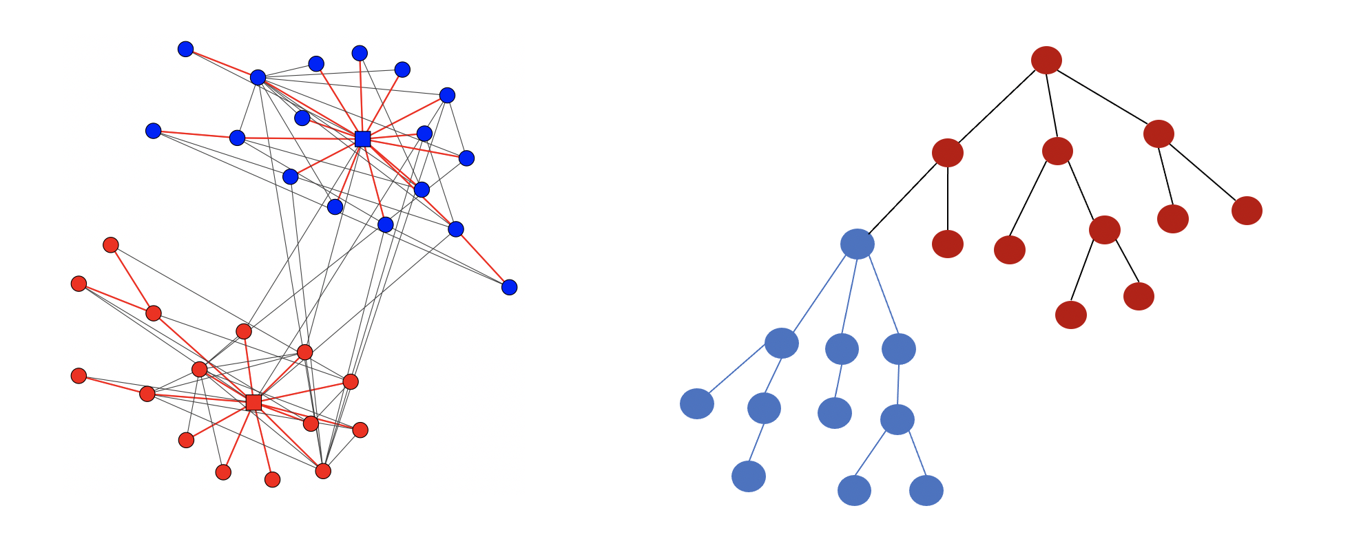
Figure 5: The karate club network (left) has two true communities. Most spanning trees of the whole karate club network would be imbalanced (such as the tree on the right), showing that the karate club network is very unlikely to have been formed from a single homogeneous growth process and hence very likely to contain multiple communities.

The PAPER model also produces more within-community edges than between-community edges because each community has a spanning tree. However, since a tree on $n$ nodes only has $n-1$ edges, the difference in the within-community edge density and the between-community edge density is diminishingly small when the noise level $\theta$ is of an order larger than $\omega(\frac{1}{n})$. In this case, the peripheral leaf nodes of a community-tree become impossible to cluster but it is still possible to recover the root node of each of the community-trees, as our experimental results show. One disadvantage of the PAPER notion of community is that it is not able to capture non-assortative clusters where nodes in the same clusters are unlikely to form edges.

The PAPER notion of community is appropriate in many application. For example, for a co-authorship network where there exists an underlying growth process, our empirical analysis in Section 6.5 shows that the PAPER model captures clusters that accurately reflect salient research communities. We can also combine both notions by a PAPER-SBM mixture model, where we generate a preferential attachment forest $\bm{F}_{n}$ via the mechanism described in Definition 4 or 5, then, for every pair of nodes $u$ and $v$, we add a noisy edge $(u,v)$ with probability $\theta_{1}$ if $u$ and $v$ belong to the same tree in $\bm{F}_{n}$ and with a different probability $\theta_{2}$ if $u$ and $v$ belong to different trees. The inference method and algorithm that we develop in this manuscript can extend to such a PAPER-SBM mixture model, but the computational run-time would be substantially slower. We relegate a detailed study of a PAPER-SBM mixture model to a future work.

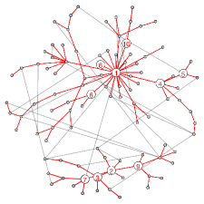
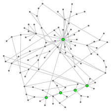
Figure 6: Left: illustration of PAPER model with $K=2$ underlying trees; nodes have latent time ordering (only first 10 orderings shown); the red edges form the latent tree while gray edges are Erdős–Rényi. Right: 80% confidence set for the set of root nodes (node number 1 for tree 1 and node number 2 for tree 2) constructed from the unlabeled graph.

2.3 Sequential noise models

As suggested in Remark 1, PAPER model is a special case of a general Markovian process over a sequence of networks $\bm{G}_{1},\bm{G}_{2},\ldots,\bm{G}_{n}$ based on a latent sequence of trees $\bm{T}_{1},\bm{T}_{2},\ldots,\bm{T}_{n}$. In the general framework, we specify the transition kernel $\mathbb{P}(\bm{G}_{t}\,|\,\bm{G}_{t-1})$ by specifying two stages:

1. (tree stage) $\mathbb{P}(\bm{T}_{t}\,|\,\bm{T}_{t-1},\bm{G}_{t-1})$ which adds one node $t$ and one tree edge and

2. (noise stage) $\mathbb{P}(\bm{G}_{t}\,|\,\bm{T}_{t},\bm{G}_{t-1})$ which adds more random edges to obtain $\bm{G}_{t}$.

We can of course define $\mathbb{P}(\bm{G}_{t}\,|\,\bm{G}_{t-1})$ without having an underlying tree but the key insight of our approach is that augmenting the model with the latent tree $\bm{T}_{n}$ greatly facilitates the design of tractable models and inference algorithms because calculations on trees are easy and fast. In addition, the latent tree has a real world interpretation as the recruitment history – a tree edge between nodes $(u,v)$ implies that node $u$ recruited node $v$ into the network.

In the noise stage, if we independently adds noise edges between the new node $t$ and the existing nodes with the same probability $\theta$, then we get back the single root PAPER model. More generally, we can let the noise edge probability depend on the time $t$ and the state of the graph at time $t$. We define the following extension which we refer to as the seq-PAPER model with parameters $(\alpha,\beta,\theta,\tilde{\alpha},\tilde{\beta})$:

Definition 6.

We start with a singleton root node $\bm{T}_{1}=\bm{G}_{1}=\{1\}$. At time $t=2$, we add node $2$ and attach it to node $1$. At time $t\geq 3:$

1. (tree stage) We add new node $t$; we select node an existing node $w_{t}\in[t-1]$ with probability $\frac{\beta D_{\bm{T}_{t-1}}(w_{t})+\alpha}{2(t-2)\beta+(t-1)\alpha}$ and add edge $(t,w_{t})$ to $\bm{T}_{t-1}$ to form $\bm{T}_{t}$;

2. (noise stage) for each existing node $j\in[t-1]$, we add edge $(t,j)$ independently with probability

   $$q_{j}:=\theta\frac{\tilde{\beta}D_{\bm{T}_{t-1}}(j)+\tilde{\alpha}}{2(t-2)\tilde{\beta}+(t-1)\tilde{\alpha}}\wedge 1.$$ (4)

   It is possible that we add the tree edge $(j,w_{t})$ in the noise stage in which case we collapse the multi-edge.

In general, we may take $\tilde{\beta}=\beta$ and $\tilde{\alpha}=\alpha$ but we allow them to be distinct in the model definition for greater flexibility. We discuss parameter estimation in Section S3.5.4 of the Appendix.

When $t$ is large, the independent Bernoulli generative process approximates a Poisson growth model (see e.g. Sheridan et al. (2008)) where we first generate $M\sim\text{Poisson}(\theta)$, and then repeat $M$ times the procedure where we draw an existing node $j\in[t-1]$ with probability $q_{j}$ (also with replacement) and then add the edge $(t,j)$ to the random network, collapsing multi-edges if any are formed. We thus add an average of approximately $\theta$ noise edges at each time step. In contrast, under the PAPER model where the noise edge probability is $\theta$, we add on average $(t-2)\cdot\theta$ noise edges at time $t$.

The approximation error between the Bernoulli mechanism and the Poisson mechanism, in each iteration $t$, converges to 0 in total variation distance as $t$ increases; see rigorous statement and proof in Proposition S4 of Section S1.2 in the Appendix. However, it is important to note that the two mechanisms could still produce final random graphs whose overall distributions have total variation distance bounded away from 0. For example, UA or LPA trees are known to be sensitive to initialization so that different initial seeds could lead to very different distributions over the final observed graph, see e.g. Bubeck et al. (2015) and curien2015scaling. In this work, we prefer the Bernoulli generative process in order to simplify the inference algorithm. Even with the Bernoulli approximation however, inference under the sequential setting is much more computationally intensive than the vanilla PAPER model.

A more realistic extension of the seq-PAPER model is to replace the tree degree $D_{\bm{T}_{t-1}}(j)$ with the graph degree $D_{\bm{G}_{t-1}}(j)$ in the noise probability 4. This small change unfortunately leads to additional significant slowdown in the resulting inference algorithm; see Remark 9 for more detail. We note that an even more sophisticated model of sequential noise is one where the additional noise edges are generated by a random walk mechanism (Bloem-Reddy and Orbanz, 2018); Bloem-Reddy and Orbanz (2018) proposes a sequential Monte Carlo inference method which may not scale well to large networks.

We have so far considered additive noise where new edges are added to the network. We can also model deletion noise where each tree edge is removed from the observed network independently with some probability $\eta>0$. Having deletion noise under the vanilla PAPER model can adversely increase the size of the confidence set for the root node. However, the seq-PAPER model is much more resilient to deletion noise, especially when $\tilde{\beta}=\beta$ and $\tilde{\alpha}=\alpha$ since the noise edges also contain sequential information. To be precisely, we define the $\text{seq-PAPER}^{*}(\alpha,\beta,\theta,\tilde{\alpha},\tilde{\beta},\eta)$ as the model where we first generate $\bm{G}_{n}$ according to the $\text{seq-PAPER}(\alpha,\beta,\theta,\tilde{\alpha},\tilde{\beta})$ model with latent spanning tree $\bm{T}_{n}$; we then remove each edge of $\bm{T}_{n}$ from the final graph $\bm{G}_{n}$ independently with probability $\eta$.

2.4 Related Work

Many researchers in statistics (Kolaczyk, 2009), computer science (Bollobás et al., 2001), engineering, and physics (Callaway et al., 2000) have been interested in the probabilistic properties of various random growth processes of networks, including the preferential attachment model (Barabási and Albert, 1999). Recently however, the specific problem of root inference on trees has received increased attention.

These efforts began with the ground-breaking work of Bubeck, Devroye and Lugosi (2017); Bubeck et al. (2015); Bubeck, Eldan, Mossel and Rácz (2017), which shows that, given an observation of an LPA or UA tree of size $n$, for any $\epsilon\in(0,1]$, one can construct asymptotically valid confidence sets for the root node with size $K_{LPA}(\epsilon)$ and $K_{UA}(\epsilon)$ for LPA or UA trees respectively. Importantly and surprisingly, $K_{LPA}(\epsilon)$ and $K_{UA}(\epsilon)$ do not depend on $n$ so that the confidence set have size that is $O(1)$. To construct the confidence sets, Bubeck, Devroye and Lugosi (2017) computes a centrality value for every node, which can for instance be based on inverse of the size of the maximum subtree of a node (a concepted sometimes called Jordan centrality on trees, different from the notion of a Jordan center, which is the node with the minimum farthest distance to the other nodes); they then sort the nodes by centrality and take the top $K(\epsilon)$ nodes where the size $K(\epsilon)$ is determined by probabilistic bounds.

Khim and Loh (2017) further extends these results to the setting of uniform attachment over an infinite regular tree. Banerjee and Bhamidi (2020) improves the analysis of Jordan centrality on trees and derives tight upper and lower bounds on the confidence set size. Devroye and Reddad (2018); Lugosi et al. (2019) study the more general problem of seed-tree inference instead of root node inference. The aforementioned results apply only to tree shaped networks but very recently, Banerjee and Huang (2021) studies confidence sets constructed from the degrees of the nodes which applies to preferential attachment models in which a fixed $m$ edges are added at every iteration. After the completion of this paper, Briend et al. (2022) propose confidence sets for the root node on a class of uniform-attachment-based general Markovian graphs by detecting anchors of double-cycle subgraphs within the network; they show the confidence set sizes to be $O(1)$ and give explicit bounds in terms of confidence level $\epsilon$.

A line of work in the physics literature also explores the problem of full or partial recovery of a tree network history (Young et al., 2019; Cantwell et al., 2019; Sreedharan et al., 2019). In computer science and engineering, researchers have studied the related problem of estimating the source of an infection spreading over a background network Shah and Zaman (2011); Fioriti et al. (2014); Shelke and Attar (2019), with approaches that range from using Jordan centers, eigenvector centrality, and belief propagation (see survey in Jiang et al. (2016)).

3 Methodology

Our approach to root inference and related problems is to randomize the node labels, which induces a posterior distribution over the latent ordering.

3.1 Label randomization

Suppose $\bm{G}_{n}$ is a time labeled graph distributed according to a PAPER model and $\bm{G}^{*}_{n}$ is the alphabetically labeled observation where $\bm{G}^{*}_{n}=\rho\bm{G}_{n}$ for some label bijection $\rho\in\text{Bi}([n],\mathcal{U}_{n})$. We may independently generate a random bijection $\Lambda\in\text{Bi}(\mathcal{U}_{n},\mathcal{U}_{n})$ and apply it to $\bm{G}^{*}_{n}$ to obtain a randomly labeled graph

$$\tilde{\bm{G}}_{n}:=\Lambda\bm{G}^{*}_{n}=\underbrace{(\Lambda\circ\rho)}_{\text{$\Pi$}}\bm{G}_{n}.$$

By defining $\Pi=\Lambda\circ\rho$, we see that $\tilde{\bm{G}}_{n}=\Pi\bm{G}_{n}$ where $\Pi$ is a random bijection drawn uniformly in $\text{Bi}([n],\mathcal{U}_{n})$ independently of $\bm{G}_{n}$ (see Figure 7). We define the randomly labeled latent forest $\tilde{\bm{F}}_{n}=\Pi\bm{F}_{n}$. We may view label randomization as an augmentation of the probability space. An outcome of a PAPER model is a time labeled graph $\bm{g}_{n}$ whereas an outcome after label randomization is a pair $(\tilde{\bm{g}}_{n},\pi)$ where $\tilde{\bm{g}}_{n}$ is an alphabetically labeled graph and $\pi$ is an ordering of the nodes. We now make two simple but important observations regarding label randomization.

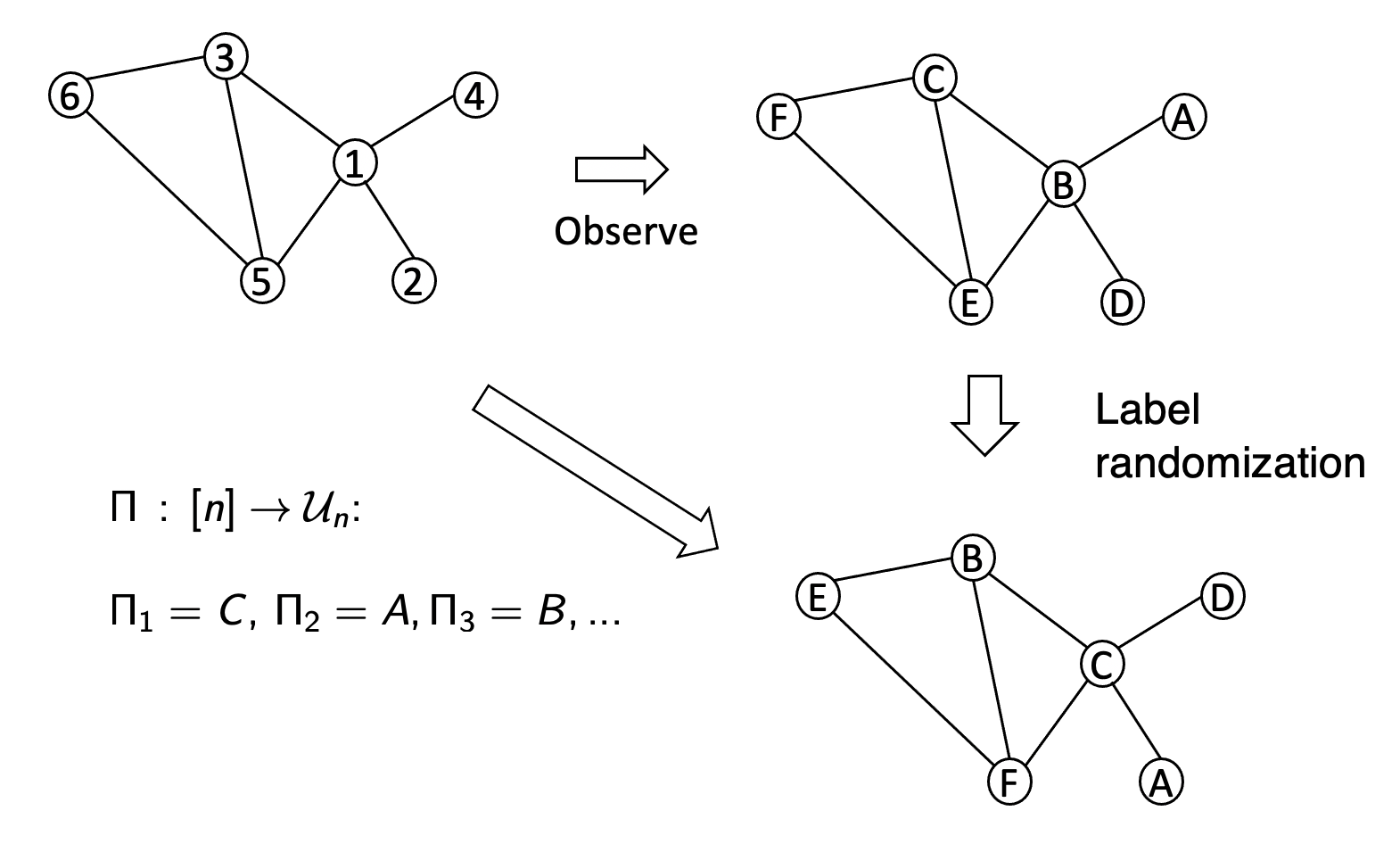
Figure 7: Label randomization induces a random latent arrival ordering $\Pi$.

Our first key observation is that, with respect to $\tilde{\bm{G}}_{n}$, the random labeling $\Pi$ describes the arrival time of the nodes in the sense that if $\Pi_{t}=u$, then the node with alphabetical label $u$ in $\tilde{\bm{G}}_{n}$ has the true arrival time $t$. Therefore, in the single root setting, we may infer the root node if we can infer $\Pi_{1}$; in the multiple roots setting, we may infer the set of root nodes if we can infer $\Pi S$.

Our second key observation is that label randomization allows us to define the posterior distribution

$$\mathbb{P}(\Pi=\pi\,|\,\tilde{\bm{G}}_{n}=\tilde{\bm{g}}_{n}) =\frac{\mathbb{P}(\tilde{\bm{G}}_{n}=\tilde{\bm{g}}_{n}\,|\,\Pi=\pi)}{\sum_{\pi^{\prime}\in\text{Bi}([n],\mathcal{U}_{n})}\mathbb{P}(\tilde{\bm{G}}_{n}=\tilde{\bm{g}}_{n}\,|\,\Pi=\pi^{\prime})}$$ (5)

which follows because $\mathbb{P}(\Pi=\pi)=\frac{1}{n!}$. This posterior distribution is supported on the subset of bijection $\pi$ such that $\pi^{-1}\tilde{\bm{g}}_{n}$ has non-zero probability under the PAPER model. In the case of the single root PAPER or seq-PAPER model, the support of (5) has a simple characterization: for every time point $t\in[n]$, define $\pi_{1:t}\cap\tilde{\bm{g}}_{n}$ as the subgraph of $\tilde{\bm{g}}_{n}$ restricted to nodes in $\pi_{1:t}$. Then, $\mathbb{P}(\Pi=\pi\,|\,\tilde{\bm{G}}_{n}=\tilde{\bm{g}}_{n})>0$ if and only if $\pi_{1:t}\cap\tilde{\bm{g}}_{n}$ is connected for all $t\in[n]$.

From a Bayesian perspective, label randomization adds a uniform prior distribution on the arrival ordering of the nodes in the observed alphabetically labeled graph $\bm{G}^{*}_{n}$; this is sometimes used in Bayesian parameter inference on network models (Sheridan et al., 2012; Bloem-Reddy et al., 2018). This prior however is not subjective. Indeed, we will see in Theorem 7 that Bayesian inference statements in our setting directly have frequentist validity as well and, from Section S2.1, that the posterior root probability of a node is equal to the likelihood of that node being the root node up to normalization.

We describe how to compute (5) tractably in Section 4. For computation, we will also be interested in the posterior probability over both the ordering $\Pi$ as well as the latent forest $\tilde{\bm{F}}_{n}$:

$$\mathbb{P}(\Pi=\pi,\tilde{\bm{F}}=\tilde{\bm{f}}_{n}\,|\,\tilde{\bm{G}}_{n}=\tilde{\bm{g}}_{n}).$$ (6)

In the single root setting, $\tilde{\bm{f}}_{n}$ is actually a tree, which we may write as $\tilde{\bm{t}}_{n}$. It is then clear that (6) is non-zero only if $\tilde{\bm{t}}_{n}$ is a spanning tree of $\tilde{\bm{g}}_{n}$, i.e., $\tilde{\bm{t}}_{n}$ is a connected subtree of $\tilde{\bm{g}}_{n}$ that contains all the vertices.

$\bm{G}_{n}$	time labeled graph (unobserved)	$\bm{F}_{n}$	latent time labeled forest
$\bm{G}^{*}_{n}$	observed alpha. labeled graph	$\bm{F}^{*}_{n}$	latent alpha. labeled forest
$\tilde{\bm{G}}_{n}$	randomly alpha. labeled graph	$\tilde{\bm{F}}_{n}$	latent randomly alpha. labeled forest
$\rho$	fixed unobserved ordering; $\bm{G}_{n}^{*}=\rho\bm{G}_{n}$	$\Pi$	latent random ordering; $\tilde{\bm{G}}_{n}=\Pi\bm{G}_{n}$
$S$	time labeled root nodes of $\bm{G}_{n}$	$\tilde{S}$	latent alpha. labeled root nodes; $\tilde{S}=\Pi S$

Table 1: Quick reference of important notation and definitions.

3.2 Confidence set for the single root

To make the ideas clear, we first consider the single root model. Since the root node is the node labeled $\Pi_{1}$ after label randomization, a natural approach is to first construct a level $1-\epsilon$ Bayesian credible set for the node $\Pi_{1}$ by using its posterior distribution, which we call the posterior root distribution.

More concretely, let $\tilde{\bm{g}}_{n}$ be an alphabetically labeled graph. For each node $u\in\mathcal{U}_{n}$ of $\tilde{\bm{g}}_{n}$, we define the posterior root probability as $\mathbb{P}(\Pi_{1}=u\,|\,\tilde{\bm{G}}_{n}=\tilde{\bm{g}}_{n})$. We sort the nodes $u_{1},\ldots,u_{n}$ so that

$$\mathbb{P}(\Pi_{1}=u_{1}\,|\,\tilde{\bm{G}}_{n}=\tilde{\bm{g}}_{n})\geq\mathbb{P}(\Pi_{1}=u_{2}\,|\,\tilde{\bm{G}}_{n}=\tilde{\bm{g}}_{n})\ldots\geq\mathbb{P}(\Pi_{1}=u_{n}\,|\,\tilde{\bm{G}}_{n}=\tilde{\bm{g}}_{n}),$$

and define

$$L_{\epsilon}(\tilde{\bm{g}}_{n})=\min\biggl{\{}k\in[n]\,:\,\sum_{i=1}^{k}\mathbb{P}(\Pi_{1}=u_{i}\,|\,\tilde{\bm{G}}_{n}=\tilde{\bm{g}}_{n})\geq 1-\epsilon\biggr{\}}$$ (7)

We then define the $\epsilon$-credible set as

$$B_{\epsilon}(\tilde{\bm{g}}_{n})=\bigl{\{}u_{1},u_{2},\ldots,u_{L_{\epsilon}(\tilde{\bm{g}}_{n})}\bigr{\}},\qquad\text{(breaking ties at random).}$$ (8)

By definition, $B_{\epsilon}(\tilde{\bm{g}})$ is the smallest set of nodes with Bayesian coverage at level $1-\epsilon$ in that $\mathbb{P}(\Pi_{1}\in B_{\epsilon}(\tilde{\bm{g}}_{n})\,|\,\tilde{\bm{G}}_{n}=\tilde{\bm{g}}_{n})\geq 1-\epsilon$. In general, credible sets do not have valid frequentist confidence coverage. However, our next theorem shows that in our setting, the credible set $B_{\epsilon}$ is in fact an honest confidence set in that $\mathbb{P}\{\text{root node}\in B_{\epsilon}(\bm{G}_{n}^{*})\}\geq 1-\epsilon$.

Theorem 7.

Let $\bm{G}_{n}\sim\text{PAPER}(\alpha,\beta,\theta)$ or $\text{seq-PAPER}(\alpha,\beta,\theta,\tilde{\alpha},\tilde{\beta})$ and let $\bm{G}^{*}_{n}$ be the alphabetically labeled observation. Let $\rho\in\text{Bi}([n],\mathcal{U}_{n})$ be any label bijection such that $\rho\mathbf{G}_{n}=\mathbf{G}^{*}_{n}$. We have that, for any $\epsilon\in(0,1)$,

$$\mathbb{P}\bigl{\{}\rho_{1}\in B_{\epsilon}(\mathbf{G}^{*}_{n})\bigr{\}}\geq 1-\epsilon.$$

The proof is very similar to that of Crane and Xu (2021, Theorem 1). Since the proof is short, we provide it here for readers’ convenience.

Proof.

We first claim that $B_{\epsilon}(\cdot)$ is labeling-equivariant (cf. Remark 4) in the sense that for any $\tau\in\text{Bi}(\mathcal{U}_{n},\mathcal{U}_{n})$ and any alphabetically labeled graph $\tilde{\bm{g}}_{n}$, we have that $\tau B_{\epsilon}(\tilde{\bm{g}}_{n})\stackrel{{\scriptstyle d}}{{=}}B_{\epsilon}(\tau\tilde{\bm{g}}_{n})$ (note that $B_{\epsilon}(\cdot)$ uses randomization to break ties). Indeed, since $(\Pi,\tilde{\bm{G}}_{n})\stackrel{{\scriptstyle d}}{{=}}(\tau^{-1}\circ\Pi,\tau^{-1}\tilde{\bm{G}}_{n})$, we have that, for any $u\in\mathcal{U}_{n}$,

$$\mathbb{P}(\Pi_{1}=u\,|\,\tilde{\bm{G}}_{n}=\tilde{\bm{g}}_{n})=\mathbb{P}(\Pi_{1}=\tau(u)\,|\,\tilde{\mathbf{G}}_{n}=\tau\tilde{\mathbf{g}}_{n}).$$

Therefore, for any $u,v\in\mathcal{U}_{n}$, we have that $\mathbf{P}(\Pi_{1}=u\,|\,\tilde{\mathbf{G}}_{n}=\tilde{\mathbf{g}}_{n})\geq\mathbf{P}(\Pi_{1}=v\,|\,\tilde{\mathbf{G}}_{n}=\tilde{\mathbf{g}}_{n})$ if and only if $\mathbf{P}(\Pi_{1}=\tau(u)\,|\,\tilde{\mathbf{G}}_{n}=\tau\tilde{\mathbf{g}}_{n})\geq\mathbf{P}(\Pi_{1}=\tau(v)\,|\,\tilde{\mathbf{G}}_{n}=\tau\tilde{\mathbf{g}}_{n})$. Since $B_{\epsilon}(\mathbf{G}^{*}_{n})$ is constructed by taking the top elements of $\mathcal{U}_{n}$ that maximize the cumulative posterior root probability, the claim follows.

Now, let $\rho\in\text{Bi}([n],\mathcal{U}_{n})$ be such that $\rho\mathbf{G}_{n}=\mathbf{G}^{*}_{n}$ and let $\Lambda$ be a random bijection drawn uniformly in $\text{Bi}(\mathcal{U}_{n},\mathcal{U}_{n})$ and let $\Pi=\Lambda\circ\rho$. Then,

$$\mathbb{P}(\rho_{1}\in B_{\epsilon}(\mathbf{G}^{*}_{n})) =\mathbb{P}(\rho_{1}\in B_{\epsilon}(\rho\mathbf{G}_{n}))$$

$$=\mathbb{P}\bigl{\{}(\Lambda\circ\rho)_{1}\in B_{\epsilon}((\Lambda\circ\rho)\mathbf{G}_{n})\,|\,\Lambda=\text{Id}\bigr{\}}$$

$$=\mathbb{P}\bigl{\{}(\Lambda\circ\rho)_{1}\in B_{\epsilon}((\Lambda\circ\rho)\mathbf{G}_{n})\bigr{\}}$$

$$=\mathbb{P}(\Pi_{1}\in B_{\epsilon}(\tilde{\mathbf{G}}_{n}))\geq 1-\epsilon,$$

where the penultimate equality follows from the labeling-equivariance of $B_{\epsilon}$ and where the last inequality follows because $\mathbf{P}(\Pi_{1}\in B_{\epsilon}(\tilde{\mathbf{G}}_{n})\,|\,\tilde{\mathbf{G}}_{n}=\tilde{\mathbf{g}}_{n})\geq 1-\epsilon$ for any labeled tree $\tilde{\mathbf{g}}_{n}$ (with labels in $\mathcal{U}_{n}$) by the definition of $B_{\epsilon}$. ∎

Remark 6.

We show in Theorem S5 of the appendix that the posterior root probability $\mathbb{P}(\Pi_{1}=u\,|\,\tilde{\bm{G}}_{n}=\tilde{\bm{g}}_{n})$ is equal to the likelihood of node $u$ being the root node on observing the unlabeled shape of $\tilde{\bm{g}}_{n}$. Therefore, the set $B_{\epsilon}(\tilde{\bm{g}}_{n})$ is in fact the maximum likelihood confidence set. Because the likelihood in this setting is complicated to even write down, we leave all the details to Section S2.1 of the appendix.

Remark 7.

One may see from the proof that Theorem 7 applies more broadly then just PAPER models. It in fact applies to any random graph $\bm{G}_{n}$ whose nodes are labeled by $\{1,2,\ldots,n\}$. For the PAPER model, the integer labels encode arrival time and thus contain information about the graph. In a model where the integer labels are uninformative of the graph connectivity structure, Theorem 7 is still valid although the posterior probability $\mathbb{P}(\Pi_{1}=\cdot\,|\,\tilde{\bm{G}}_{n}=\tilde{\bm{g}}_{n})$ would be uniform. A reviewer of this paper also pointed out that Theorem 7 is related to the classical literature on invariant/equivariant estimation where credible sets constructed from uniform (Haar) priors may also be valid confidence sets; see e.g. schervish2012theory.

3.3 Confidence set for local roots

First consider the fixed $K$ setting where $\bm{G}_{n}\sim\text{PAPER}(\alpha,\beta,\theta,K)$; let $\Pi$ be a uniformly random ordering in $\text{Bi}([n],\mathcal{U}_{n})$ and let $\tilde{\bm{G}}_{n}=\Pi\bm{G}_{n}$. The latent set of root nodes of $\tilde{\bm{G}}_{n}$ in this case is $\tilde{S}:=\Pi S=\{\Pi_{1},\ldots,\Pi_{K}\}$. We then define the posterior root probability for any node $u\in\mathcal{U}_{n}$ as

$$\mathbb{P}(u\in\tilde{S}\,|\,\tilde{\bm{G}}_{n}=\tilde{\bm{g}}_{n}),$$

that is, the probability that node $u$ is an element of the latent root set $\tilde{S}$.

To form the credible set $B_{\epsilon}(\tilde{\bm{g}}_{n})\subseteq\mathcal{U}_{n}$, we sort the nodes by the posterior root probabilities

$$\mathbb{P}(u_{1}\in\tilde{S}\,|\,\tilde{\bm{G}}_{n}=\tilde{\bm{g}}_{n})\geq\mathbb{P}(u_{2}\in\tilde{S}\,|\,\tilde{\bm{G}}_{n}=\tilde{\bm{g}}_{n})\geq\ldots\geq\mathbb{P}(u_{n}\in\tilde{S}\,|\,\tilde{\bm{G}}_{n}=\tilde{\bm{g}}_{n}).$$ (9)

We may then take $B_{\epsilon}(\tilde{\bm{g}}_{n})$ to be the smallest set of nodes such that $P\bigl{(}\tilde{S}\subsetneq B_{\epsilon}(\tilde{\bm{g}}_{n})\,|\,\tilde{\bm{G}}_{n}=\tilde{\bm{g}}_{n}\bigr{)}\leq\epsilon$. More precisely, define the integer

$$L_{\epsilon}(\tilde{\bm{g}}_{n})=\min\biggl{\{}k\in[n]\,:\, \sum_{i=k+1}^{n}\mathbb{P}(u_{i}\in\tilde{S}\,|\,\tilde{\bm{G}}_{n}=\tilde{\bm{g}}_{n})\leq\epsilon\biggr{\}}$$ (10)

and then define the credible set as

$$B_{\epsilon}(\tilde{\bm{g}}_{n})=\bigl{\{}u_{1},u_{2},\ldots,u_{L_{\epsilon}(\tilde{\bm{g}}_{n})}\bigr{\}}\qquad\text{(breaking ties at random).}$$ (11)

In the $\text{PAPER}(\alpha,\beta,\alpha_{0},\theta)$ model where the number of roots $K$ is random, the set of root nodes is $\tilde{S}=\Pi S$ which comprises, according to the ordering $\Pi$, of the node that is first to arrive in each of the component trees of $\tilde{\bm{F}}_{n}$. We may then sort the nodes as in (9), compute $L_{\epsilon}(\tilde{\bm{g}}_{n})$ as in (10) and $B_{\epsilon}(\tilde{\bm{g}}_{n})$ as in (11).

Similar to Theorem 7, we may show that $B_{\epsilon}(\cdot)$ in fact also has frequentist coverage at the same level $1-\epsilon$.

Theorem 8.

Let $\bm{G}_{n}\sim\text{PAPER}(\alpha,\beta,K,\theta)$ or $\text{PAPER}(\alpha,\beta,\alpha_{0},\theta)$ and let $\bm{G}^{*}_{n}$ be the alphabetically labeled observation. Let $\rho\in\text{Bi}([n],\mathcal{U}_{n})$ be any label bijection such that $\rho\mathbf{G}_{n}=\mathbf{G}^{*}_{n}$ and let $S\subset[n]$ be the time labels of the root nodes (see Definitions 4 and 5). We have that, for any $\epsilon\in(0,1)$,

$$\mathbb{P}\bigl{\{}\rho S\subseteq B_{\epsilon}(\mathbf{G}^{*}_{n})\bigr{\}}\geq 1-\epsilon.$$

Proof.

The proof is very similar to that of Theorem 7. First, since the random set $\tilde{S}$ is a function of the random ordering $\Pi$ in the fixed $K$ setting and a function of both the random ordering $\Pi$ and the random forest $\tilde{\bm{F}}_{n}$, we write $\tilde{S}(\Pi)$ or $\tilde{S}(\Pi,\tilde{\bm{F}}_{n})$ to be precise.

We then observe that $\tilde{S}(\Pi)$ in the fixed $K$ setting or $\tilde{S}(\Pi,\tilde{\bm{F}}_{n})$ in the random $K$ setting, are labeling equivariant in that for any $\tau\in\text{Bi}(\mathcal{U}_{n},\mathcal{U}_{n})$, we have that $\tilde{S}(\tau^{-1}\Pi)=\tau^{-1}\tilde{S}(\Pi)$ or, in the random $K$ setting, $\tilde{S}(\tau^{-1}\Pi,\tau^{-1}\tilde{\bm{F}}_{n})=\tau^{-1}\tilde{S}(\Pi,\tilde{\bm{F}}_{n})$. Therefore, since $(\Pi,\tilde{\bm{G}}_{n})\stackrel{{\scriptstyle d}}{{=}}(\tau^{-1}\Pi,\tau^{-1}\tilde{\bm{G}}_{n})$ for any $\tau\in\text{Bi}(\mathcal{U}_{n},\mathcal{U}_{n})$, we have $\tilde{S}(\Pi,\tilde{\bm{F}}_{n})\stackrel{{\scriptstyle d}}{{=}}\tau^{-1}\tilde{S}(\Pi,\tilde{\bm{F}}_{n})$ and thus, for any $u\in\mathcal{U}_{n}$,

$$\mathbb{P}(u\in\tilde{S}\,|\,\tilde{\bm{G}}_{n}=\tilde{\bm{g}}_{n})=\mathbb{P}(\tau(u)\in\tilde{S}\,|\,\tilde{\bm{G}}_{n}=\tau\tilde{\bm{g}}_{n}).$$

The rest the proof proceeds in an identical manner to that of Theorem 7. ∎

When there are multiple roots, an alternative way of inferring the root set is to construct the confidence set $B_{\epsilon}(\cdot)$ as a set of subsets of the nodes and then require that $\tilde{S}\in B_{\epsilon}$ with probability at least $1-\epsilon$. We can take the same approach to construct such confidence set over sets but it becomes much more computationally intensive to compute them in practice.

3.4 Combinatorial interpretation

Before we describe the Gibbs sampling algorithm for computing the posterior root probabilities $\mathbb{P}(\Pi_{1}=u\,|\,\tilde{\bm{G}}_{n}=\tilde{\bm{g}}_{n})$, we provide an intuitive combinatorial interpretation of the posterior root probability in the single root PAPER model (Definition 2). The definitions and calculations here are also important for deriving the algorithm in Section 4.

The noiseless case: We first consider the simpler setting in which we can observe the tree $\tilde{\bm{T}}_{n}$ (with a single root) distributed according to the APA model. In this case, we have

$$\mathbb{P}(\Pi_{1}=\cdot\,|\,\tilde{\bm{T}}_{n}=\tilde{\bm{t}}_{n})=\sum_{\pi\,:\,\pi_{1}=u}\mathbb{P}(\Pi=\pi\,|\,\tilde{\bm{T}}_{n}=\tilde{\bm{t}}_{n}).$$

Recall that $\tilde{\bm{T}}_{n}=\Pi\bm{T}_{n}$ where $\bm{T}_{n}$ is a random time labeled tree with $\text{APA}(\alpha,\beta)$ distribution and $\Pi$ is an independent uniformly random ordering in $\text{Bi}([n],\mathcal{U}_{n})$. The distribution $\mathbb{P}(\Pi=\pi\,|\,\tilde{\bm{T}}_{n}=\tilde{\bm{t}}_{n})$ is supported on a subset of the the bijections $\text{Bi}([n],\mathcal{U}_{n})$ because $\pi^{-1}\tilde{\bm{T}}_{n}$ must be a valid time labeled tree (also called recursive tree in discrete mathematics). To be precise, we define the histories of $\tilde{\bm{t}}_{n}$ as

$$\text{hist}(\tilde{\bm{t}}_{n}) :=\bigl{\{}\pi\in\text{Bi}([n],\mathcal{U}_{n})\,:\,\mathbb{P}(\bm{T}_{n}=\pi^{-1}\tilde{\bm{t}}_{n})>0\bigr{\}},\text{ and }$$

$$h(\tilde{\bm{t}}_{n}) :=|\text{hist}(\tilde{\bm{t}}_{n})|$$

as the number of distinct histories. Since the APA tree distribution assigns a non-zero probability to any valid time labeled trees, we see that $\text{hist}(\tilde{\bm{t}}_{n})$ contains the elements $\pi$ of $\text{Bi}([n],\mathcal{U}_{n})$ such that for all $t\in[n]$, the subtree restricted only to nodes in $\pi_{1:t}$, i.e. $\tilde{\bm{t}}_{n}\cap\pi_{1:t}$, is connected. Thus, $\text{hist}(\tilde{\bm{t}}_{n})$ is the set of bijections $\pi$ which represent a valid arrival ordering for the nodes of the given tree $\tilde{\bm{t}}_{n}$. Similarly, we define, for any node $u\in\mathcal{U}_{n}$,

$$\text{hist}(u,\tilde{\bm{t}}_{n}):=\bigl{\{}\pi\in\text{hist}(\tilde{\bm{t}}_{n})\,:\,\pi_{1}=u\bigr{\}}$$

$$h(u,\tilde{\bm{t}}_{n}):=|\text{hist}(u,\tilde{\bm{t}}_{n})|,$$

as histories of $\tilde{\bm{t}}_{n}$ that start at node $u$. We illustrate an example of the set of histories for a simple tree in Figure 8.

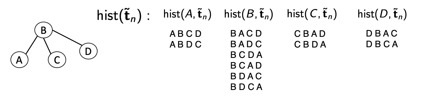
Figure 8: All histories of a tree with 4 nodes.

By definition, $\mathbb{P}(\Pi=\cdot\,|\,\tilde{\bm{T}}_{n}=\tilde{\bm{t}}_{n})$ is supported on $\text{hist}(\tilde{\bm{t}}_{n})$. For most values of $\alpha$ and $\beta$, the posterior distribution is in fact uniform over $\text{hist}(\tilde{\bm{t}}_{n})$:

Proposition 9.

(Crane and Xu, 2021, Theorem 4 and Proposition 3) Let $\alpha,\beta$ be two real numbers such that either (1) $\beta\geq 0$ and $\alpha\geq-\beta$ or (2) $\beta<0$ and $\alpha=-D\beta$ for some integer $D\geq 2$. Suppose $\bm{T}_{n}\sim\text{APA}(\alpha,\beta)$. Let $\Pi$ be a uniformly random ordering taking value in $\text{Bi}([n],\mathcal{U}_{n})$ and let $\tilde{\bm{T}}_{n}=\Pi\bm{T}_{n}$. Then,

$$\mathbb{P}(\Pi=\pi\,|\,\tilde{\bm{T}}_{n}=\tilde{\bm{t}}_{n})=\frac{1}{h(\tilde{\bm{t}}_{n})}\mathbbm{1}\{\pi\in\text{hist}(\tilde{\bm{t}}_{n})\}.$$ (12)

The full proof of Proposition 9 is in Crane and Xu (2021) but we give a short justification here: the posterior is uniform because $\mathbb{P}(\Pi=\pi\,|\,\tilde{\bm{T}}_{n}=\tilde{\bm{t}}_{n})=\frac{\mathbb{P}(\tilde{\bm{T}}_{n}=\tilde{\bm{t}}_{n}\,|\,\Pi=\pi)\frac{1}{n!}}{\mathbb{P}(\tilde{\bm{T}}_{n}=\tilde{\bm{t}}_{n})}=\frac{\mathbb{P}(\bm{T}_{n}=\pi^{-1}\tilde{\bm{t}}_{n})\frac{1}{n!}}{\mathbb{P}(\tilde{\bm{T}}_{n}=\tilde{\bm{t}}_{n})}$. Moreover, the probability $\mathbb{P}(\bm{T}_{n}=\pi^{-1}\tilde{\bm{t}}_{n})$ is actually the same for any $\pi\in\text{hist}(\tilde{\bm{t}}_{n})$ by Proposition S1.

By Proposition 9, we have that

$$\mathbb{P}(\Pi_{1}=u\,|\,\tilde{\bm{T}}_{n}=\tilde{\bm{t}}_{n}) =\frac{h(u,\tilde{\bm{t}}_{n})}{h(\tilde{\bm{t}}_{n})}.$$

Therefore, we need only count the histories $h(u,\tilde{\bm{t}}_{n})$ for every node $u\in\mathcal{U}_{n}$. We give a well-known characterization of $h(u,\tilde{\bm{t}}_{n})$ that leads to a linear time algorithm for counting the size of the histories: define, for any node $u,v\in\mathcal{U}_{n}$, the tree $\tilde{\bm{t}}_{v}^{(u)}$ as the subtree of node $v$ where we view the whole tree as being rooted (hanging from) node $u$; $\tilde{\bm{t}}^{(u)}_{u}$ is thus the entire tree rooted at $u$. See Figure 9 for an example. We then have that, by Knuth (1997) or Shah and Zaman (2011),

$$h(u,\tilde{\bm{t}}_{n})=n!\prod_{v\in\mathcal{U}_{n}}\frac{1}{|\tilde{\bm{t}}^{(u)}_{v}|}.$$ (13)

Therefore, we can compute $h(u,\tilde{\bm{t}}_{n})$ by viewing $\tilde{\bm{t}}_{n}$ as being rooted at $u$ and taking the product of the inverse of the sizes of all the subtrees. By using the fact that $h(u,\tilde{\bm{t}}_{n})$ can be directly computed from $h(u^{\prime},\tilde{\bm{t}}_{n})$ for any neighbor $u^{\prime}$ of $u$, Shah and Zaman (2011) derive an $O(n)$ algorithm for computing the size of the histories over all roots $\{h(u,\tilde{\bm{t}}_{n})\}_{u\in\mathcal{U}_{n}}$, which we give in Section S2 of the appendix for readers’ convenience.

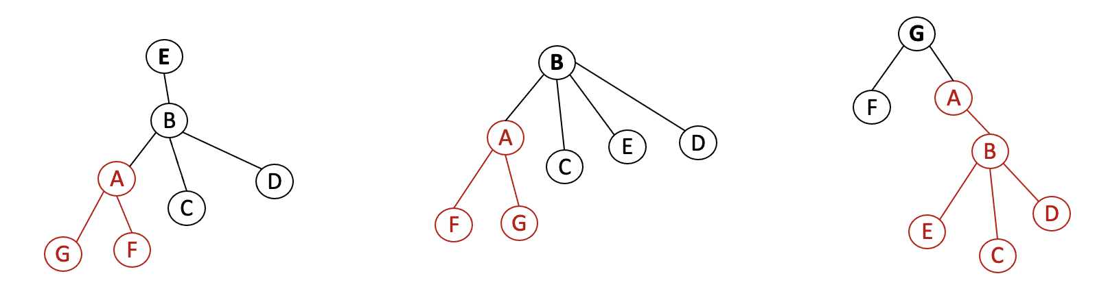
Figure 9: Same tree $\tilde{\bm{t}}_{n}$ in three rooted orientations. Left: $\tilde{\bm{t}}_{n}^{(E)}$ rooted at $E$; the subtree of $A$ (denoted $\tilde{\bm{t}}^{(E)}_{A}$) contains nodes $A,F,G$; node $A$ is the parent of $F,G$. Center: $\tilde{\bm{t}}_{n}^{(B)}$ rooted at $B$; the subtree of $A$ (denoted $\tilde{\bm{t}}^{(B}_{A}$) contains nodes $A,F,G$; node $A$ is the parent of $F,G$. Right: $\tilde{\bm{t}}_{n}^{(G)}$ rooted at $G$; the subtree of $A$ (denoted $\tilde{\bm{t}}^{(G)}_{A}$) contains nodes $A,B,E,C,D$; node $A$ is the parent of $B$.

The general case: Now suppose we have the label randomized graph $\tilde{\bm{G}}_{n}$ from the PAPER model. We then have that

$$\mathbb{P}(\Pi_{1}=u\,|\,\tilde{\bm{G}}_{n}=\tilde{\bm{g}}_{n}) =\sum_{\tilde{\bm{t}}_{n}\subseteq\tilde{\bm{g}}_{n}}\sum_{\pi\in\text{hist}(u,\tilde{\bm{t}}_{n})}\mathbb{P}(\Pi=\pi,\tilde{\bm{T}}_{n}=\tilde{\bm{t}}_{n}\,|\,\tilde{\bm{G}}_{n}=\tilde{\bm{g}}_{n})$$

$$\propto\sum_{\tilde{\bm{t}}_{n}\subseteq\tilde{\bm{g}}_{n}}\sum_{\pi\in\text{hist}(u,\tilde{\bm{t}}_{n})}\mathbb{P}(\Pi=\pi,\tilde{\bm{T}}_{n}=\tilde{\bm{t}}_{n})\underbrace{\mathbb{P}(\tilde{\bm{G}}_{n}=\tilde{\bm{g}}_{n}\,|\,\tilde{\bm{T}}_{n}=\tilde{\bm{t}}_{n},\Pi=\pi)}_{\binom{n(n-1)/2-(n-1)}{m-(n-1)}^{-1}}.$$

$$\propto\sum_{\tilde{\bm{t}}_{n}\subseteq\tilde{\bm{g}}_{n}}\sum_{\pi\in\text{hist}(u,\tilde{\bm{t}}_{n})}\mathbb{P}(\tilde{\bm{T}}_{n}=\tilde{\bm{t}}_{n}\,|\,\Pi=\pi)=\sum_{\tilde{\bm{t}}\subseteq\tilde{\bm{g}}_{n}}\sum_{\pi\in\text{hist}(u,\tilde{\bm{t}})}\mathbb{P}(\bm{T}_{n}=\pi^{-1}\tilde{\bm{t}}_{n}),$$ (14)

where, in the outer summation, we require $\tilde{\bm{t}}_{n}$ to be a subtree of $\tilde{\bm{g}}_{n}$ with $n$ nodes, that is, we require $\tilde{\bm{t}}_{n}$ to be a spanning tree of $\tilde{\bm{g}}_{n}$ (see (16)). If $\bm{T}_{n}$ has the uniform attachment distribution ($\alpha=1,\beta=0$), then we have that $\mathbb{P}(\bm{T}_{n}=\pi^{-1}\tilde{\bm{t}}_{n})=\frac{1}{(n-1)!}$ by Proposition S1 and hence,

$$\mathbb{P}(\Pi_{1}=u\,|\,\tilde{\bm{G}}_{n}=\tilde{\bm{g}}_{n})\propto\sum_{\tilde{\bm{t}}_{n}\subseteq\tilde{\bm{g}}_{n}}h(u,\tilde{\bm{t}}_{n}).$$

Thus, the posterior root probability of $u$ is simply proportional to the number of all possible realizations of growth process that start from node $u$ and end up with graph $\tilde{\bm{g}}_{n}$; see Figure 10. When $\bm{T}_{n}$ has the LPA distribution $(\alpha=0,\beta=1)$, then $\mathbb{P}(\bm{T}_{n}=\pi^{-1}\tilde{\bm{t}}_{n})$ depends on the degree sequence of the tree $\tilde{\bm{t}}_{n}$ so that the posterior root probability is proportional to a weighted count of all possible growth realizations.

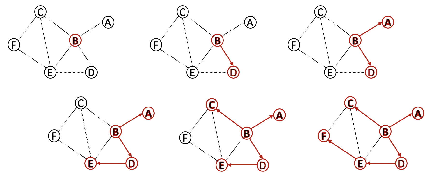
Figure 10: One possible growth realization starting from node B.

4 Algorithm

The inference approach that we described in Sections 3.2 and 3.3 requires computing posterior probabilities such as the posterior root probability $P(\Pi_{1}=u\,|\,\tilde{\bm{G}}_{n}=\tilde{\bm{g}}_{n})$ for a fixed alphabetically labeled graph $\tilde{\bm{g}}_{n}$. In this section, we derive a Gibbs sampling algorithm to generate an ordering $\pi\in\text{Bi}([n],\mathcal{U}_{n})$ and a forest $\tilde{\bm{f}}_{n}$ according to the posterior probability

$$\mathbb{P}(\Pi=\pi,\tilde{\bm{F}}_{n}=\tilde{\bm{f}}_{n}\,|\,\tilde{\bm{G}}_{n}=\tilde{\bm{g}}_{n}).$$ (15)

As discussed towards the end of Section 3.1, in the single root setting, the posterior probability (15) over $\Pi,\tilde{\bm{F}}_{n}$ is non-zero only if $\tilde{\bm{f}}_{n}$ is a spanning tree of the graph $\tilde{\bm{g}}_{n}$. We formally define the set of spanning trees of a connected graph $\tilde{\bm{g}}_{n}$ as

$$\mathcal{T}(\tilde{\bm{g}}_{n}):=\bigl{\{}\tilde{\bm{f}}_{n}\,:\,\text{$\tilde{\bm{f}}_{n}$ is connected subtree of $\tilde{\bm{g}}_{n}$ and $V(\tilde{\bm{f}}_{n})=V(\tilde{\bm{g}}_{n})$}\bigr{\}}.$$ (16)

We note that $\mathcal{T}(\tilde{\bm{g}}_{n})$ is non-empty if and only if $\tilde{\bm{g}}_{n}$ is connected. For the multiple roots setting, we define the spanning forest of $\tilde{\bm{g}}_{n}$ with $K$ components as

$$\mathcal{F}_{K}(\tilde{\bm{g}}_{n}):=\bigl{\{}\tilde{\bm{f}}_{n}\,:\,\text{$\tilde{\bm{f}}_{n}$ is sub-forest of $\tilde{\bm{g}}_{n}$ with $K$ disjoint component trees and $V(\tilde{\bm{f}}_{n})=V(\tilde{\bm{g}}_{n})$}\bigr{\}}$$

so that $\mathcal{F}_{1}(\tilde{\bm{g}}_{n})=\mathcal{T}(\tilde{\bm{g}}_{n})$. Then, for the fixed $K$ roots model, the posterior probability (15) is non-zero only if $\tilde{\bm{f}}_{n}\in\mathcal{F}_{K}(\tilde{\bm{g}}_{n})$ and for the random $K$ roots model, probability (15) is non-zero only if $\tilde{\bm{f}}_{n}\in\mathcal{F}(\tilde{\bm{g}}_{n}):=\cup_{K=1}^{n}\mathcal{F}_{K}(\tilde{\bm{g}}_{n})$.

The value of the posterior probability (15) depends on the parameters of the model, e.g. $\alpha,\beta,\theta$ in the single root setting. We provide an estimation procedure for these parameters in Section S3.1 but for now, to keep the presentation simple, we assume that all parameters are known.

Our Gibbs sampler alternates between two stages:

1. We fix the forest $\tilde{\bm{f}}_{n}$ and generate an ordering $\pi$ with probability $\mathbb{P}(\Pi=\pi\,|\,\tilde{\bm{G}}_{n}=\tilde{\bm{g}}_{n},\tilde{\bm{F}}_{n}=\tilde{\bm{f}}_{n})$.

2. We fix the ordering $\pi$ and generate a new forest $\tilde{\bm{f}}_{n}$ by iteratively sampling a new parent for each of the nodes.

We give the details for stage A in the next section and for stage B in Section 4.2.

Remark 8.

In Section S3.3, we give an alternative collapsed Gibbs sampling algorithm in which we collapse stage (A) so that we only sample the roots instead of the whole history $\pi$. The collapsed Gibbs sampler requires fewer iterations to converge but each iteration is more computationally intensive. Practically, the sampling algorithm that we present in Section 4.1 and 4.2 appears to be faster except for the random $K$ roots model on some data sets.

4.1 Sampling the ordering

In this section, we provide an algorithm for the first stage of the Gibbs sampler where we sample an ordering. We fix a spanning forest $\tilde{\bm{f}}_{n}$ of the observed graph $\tilde{\bm{g}}_{n}$, let $K$ be the number of component trees of $\tilde{\bm{f}}_{n}$, and let $m=|E(\tilde{\bm{g}}_{n})|$ be the number of edges of $\bm{g}_{n}$. We have that

$$\mathbb{P}(\Pi=\pi\,|\,\tilde{\bm{G}}_{n}=\tilde{\bm{g}}_{n},\tilde{\bm{F}}_{n}=\tilde{\bm{f}}_{n})\propto\mathbb{P}(\Pi=\pi\,|\,\tilde{\bm{F}}_{n}=\tilde{\bm{f}}_{n})\mathbb{P}(\tilde{\bm{G}}_{n}=\tilde{\bm{g}}_{n}\,|\,\tilde{\bm{F}}_{n}=\tilde{\bm{f}}_{n},\Pi=\pi).$$ (17)

Under the non-sequential noise PAPER models, since the non-forest edges of $\tilde{\bm{G}}_{n}$ are independent Erdős–Rényi random edges, we have $\mathbb{P}(\tilde{\bm{G}}_{n}=\tilde{\bm{g}}_{n}\,|\,\tilde{\bm{F}}_{n}=\tilde{\bm{f}}_{n},\Pi=\pi)=\binom{\binom{n}{2}-(n-K)}{m-(n-K)}^{-1}$ and may thus ignore the non-forest edges and consider only on the posterior probability $\mathbb{P}(\Pi=\pi\,|\,\tilde{\bm{F}}_{n}=\tilde{\bm{f}}_{n})$ when sampling $\pi$. In the sequential noise seq-PAPER model, the $\mathbb{P}(\tilde{\bm{G}}_{n}=\tilde{\bm{g}}_{n}\,|\,\tilde{\bm{F}}_{n}=\tilde{\bm{f}}_{n},\Pi=\pi)$ term must be taken into account but can be computed efficiently. We give the detailed algorithms for each of the settings.

Single root setting: In the single root setting, $\tilde{\bm{f}}_{n}$ is connected and hence a tree; we thus change to the notation $\tilde{\bm{t}}_{n}:=\tilde{\bm{f}}_{n}$ to be consistent with the notation used in Definition 1.

Hence, by our discussion in Section 3.4, sampling $\pi$ according to $\mathbb{P}(\Pi=\cdot\,|\,\tilde{\bm{T}}_{n}=\tilde{\bm{t}}_{n})$ is equivalent to sampling $\pi$ uniformly from $\text{hist}(\tilde{\bm{t}}_{n})$. Crane and Xu (2021) and also Cantwell et al. (2021) derive a procedure to sample uniformly from $\text{hist}(\tilde{\bm{t}}_{n})$ and we provide a concise description of the procedure here for the readers’ convenience.

To generate $\pi$ uniformly from $\text{hist}(\tilde{\bm{t}}_{n})$, we generate the first node $\pi_{1}$ by taking the set of all nodes and drawing a node $u$ with probability

$$\mathbb{P}(\Pi_{1}=u\,|\,\tilde{\bm{T}}_{n}=\tilde{\bm{t}}_{n})=\frac{h(u,\tilde{\bm{t}}_{n})}{h(\tilde{\bm{t}}_{n})}.$$ (18)

The entire collection $\{h(u,\tilde{\bm{t}}_{n})\}_{u\in\mathcal{U}_{n}}$ can be computed in $O(n)$ time (c.f. Section 3.4 and S2) and thus we require at most $O(n)$ time to generate the first node $\pi_{1}$.

To generate the subsequent ordering $\pi_{2:n}$, we view the tree $\tilde{\bm{t}}_{n}$ as being rooted at $\pi_{1}$ and use the notation $\tilde{\bm{t}}_{n}^{(\pi_{1})}$ make the root explicit. For each node $v\in\mathcal{U}_{n}$, we define $\tilde{\bm{t}}_{v}^{(\pi_{1})}$ as the subtree of the node $v$, viewing the whole tree as being rooted at node $\pi_{1}$. We give an example of these definitions in Figure 9.

Then, by Crane and Xu (Proposition 9 2021), for every $t\in[n-1]$,

$$\mathbb{P}(\Pi_{t+1}=v\,|\,\tilde{\bm{T}}_{n}=\tilde{\bm{t}}_{n},\Pi_{1:t}=\pi_{1:t}) =\left\{\begin{array}[]{cc}\frac{|\tilde{\bm{t}}^{(\pi_{1})}_{v}|}{n-t+1}&\text{ if $v$ is a neighbor of $\pi_{1:t}$ in $\tilde{\bm{t}}_{n}$}\\ 0&\text{ else}\end{array}\right.$$ (21)

One may verify this by showing that the probability of generating a particular ordering is $\frac{1}{n!}\prod_{v\in\mathcal{U}_{n}}|\tilde{\bm{t}}_{n}^{(u)}|=\frac{1}{h(u,\tilde{\bm{t}}_{n})}$ by (13).

Thus, we may generate $\pi_{2}$ by considering all neighbors of $\pi_{1}$ in $\tilde{\bm{t}}_{n}$ and drawing a node $v$ with probability proportional to the size of its subtree $|\tilde{\bm{t}}^{(u_{1})}_{v}|$ and similar for $\pi_{3}$, $\pi_{4}$, etc. The entire sampling process can be efficiently done by generating a permutation uniformly at random and modifying it in place so that it obeys the $\text{hist}(\tilde{\bm{f}}_{n})$ constraint. We summarize this in Algorithm 1 with $K=1$ and also give a visual illustration in Figure 11. The runtime of the sampling algorithm is upper bounded by $O(n\text{diam}(\tilde{\bm{t}}_{n}))$ (Crane and Xu, 2021, Proposition 10). Trees generated by the $\text{APA}(\alpha,\beta)$ model have diameter $O_{p}(\log n)$ (see e.g. Drmota (2009, Theorem 6.32) and Bhamidi (2007, Theorem 18)) and the overall runtime is therefore $O(n\log n)$. The computational complexity is the same under the fixed $K$ setting and the random $K$ setting.

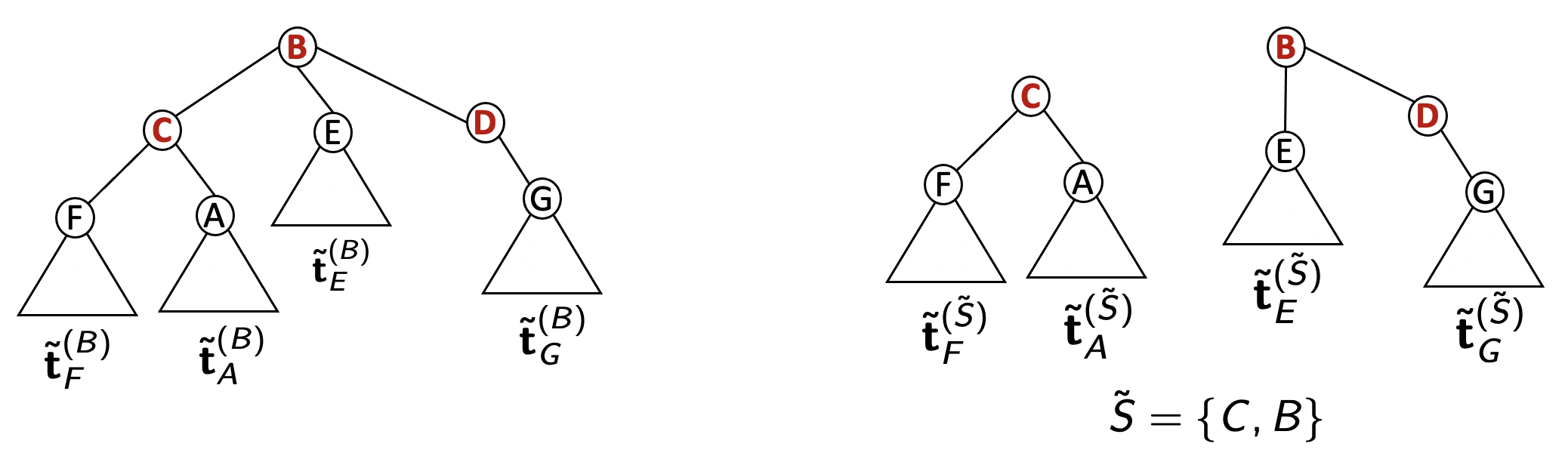
Figure 11: Example of sampling an ordering. In both cases, suppose $\pi_{1:3}=\{B,C,D\}$, then draw $\pi_{4}$ from the neighbors $\{F,A,E,G\}$ with probability proportional to the size of their subtrees.

Fixed $K$ roots setting: For the $\text{PAPER}(\alpha,\beta,K,\theta)$ model, we may generate from $\mathbb{P}(\Pi=\cdot\,|\,\tilde{\bm{F}}_{n}=\tilde{\bm{f}}_{n})$ in a similar way. In this case, $\tilde{\bm{f}}_{n}$ is a forest that contains $K$ disjoint component trees, which we denote by $\tilde{\bm{t}}^{1},\ldots,\tilde{\bm{t}}^{K}$. We first generate a root for each component tree. For each $k\in[K]$, we draw $u^{k}\in V(\tilde{\bm{t}}^{k})$ with probability

$$\frac{h(u^{k},\tilde{\bm{t}}^{k})(\beta D_{\tilde{\bm{t}}^{k}}(u^{k})+\beta+\alpha)(\beta D_{\tilde{\bm{t}}^{k}}(u^{k})+\alpha)}{\sum_{v\in V(\tilde{\bm{t}}^{k})}h(v,\tilde{\bm{t}}^{k})(\beta D_{\tilde{\bm{t}}^{k}}(v)+\beta+\alpha)(\beta D_{\tilde{\bm{t}}^{k}}(v)+\alpha)}.$$ (22)

We note that (22) is different from the corresponding probability in the single tree setting (18) because we give each root node an imaginary self-loop edge. We leave the detailed derivation of (22) to Section S3.2 of the appendix.

We let $\tilde{s}=\{u^{1},\ldots,u^{k}\}$ denote the set of roots that we have generated. By the definition of the $\text{PAPER}(\alpha,\beta,K,\theta)$ model (Definition 4), the root nodes $\tilde{s}$ occupy the first $K$ positions of the ordering $\pi$ and we thus let $\pi_{1:K}$ be the elements of $\tilde{s}$ placed in a random ordering.

Next, we view each component tree $\tilde{\bm{t}}^{k}$ as being rooted at $u_{k}$ and, for every node $v\in V(\tilde{\bm{f}}_{n})$, we denote the subtree of node $v$ by $\tilde{\bm{t}}_{v}^{(\tilde{s})}$. We then generate $\pi_{(K+1):n}$ according to probability (21) where we use the size of the subtree $|\tilde{\bm{t}}^{(\tilde{s})}_{v}|$. This is equivalent to generating a full history (excluding the root node) for every tree and then interleaving them at random. We again summarize the whole procedure in Algorithm 1.

Random $K$ roots setting: Now consider the random $K$ roots setting with the $\text{PAPER}(\alpha,\beta,\alpha_{0},\theta)$ model and suppose $\tilde{\bm{f}}_{n}$ comprises of $K$ disjoint trees $\tilde{\bm{t}}^{1},\ldots,\tilde{\bm{t}}^{K}$. We again generate the set of roots $\tilde{s}=\{u^{1},\ldots,u^{K}\}$ by drawing $u^{k}$ from $\tilde{\bm{t}}^{k}$ with probability (22). In contrast with the fixed $K$ roots setting, the root nodes $u^{1},\ldots,u^{K}$ need not occupy the first $K$ positions of the ordering $\pi$.

To generate the ordering $\pi$, we first choose $u^{k}\in\tilde{s}$ with probability $|\tilde{\bm{t}}^{k}|$ and set $\pi_{1}=u^{k}$. We then draw $\pi_{2:n}$ iteratively using the conditional distribution

$$\mathbb{P}(\Pi_{t+1}=v\,|\,\tilde{\bm{F}}_{n}=\tilde{\bm{f}},\Pi_{1:t}=\pi_{1:t}) =\left\{\begin{array}[]{cc}\frac{|\tilde{\bm{t}}^{(\tilde{s})}_{v}|}{n-t+1}&\text{ if $v$ is a neighbor of $\pi_{1:t}$ in $\tilde{\bm{f}}_{n}$ or if $v\in\tilde{s}$}\\ 0&\text{ else}\end{array}\right.$$ (25)

We note that for a root node $u^{k}\in\tilde{s}$, the subtree $\tilde{\bm{t}}^{(\tilde{s})}_{u^{k}}$ is precisely the whole tree $\tilde{\bm{t}}^{k}$. We summarize this procedure in Algorithm 1.

Sequential noise setting: Under the seq-PAPER model described in Section 2.3, we no longer have a direct sampling algorithm to draw from $\mathbb{P}(\Pi=\cdot\,|\,\tilde{\bm{G}}_{n}=\tilde{\bm{g}}_{n},\tilde{\bm{T}}_{n}=\tilde{\bm{t}}_{n})$ because we have to take into account the $\mathbb{P}(\tilde{\bm{G}}_{n}=\tilde{\bm{g}}_{n}\,|\,\tilde{\bm{T}}_{n}=\tilde{\bm{t}}_{n},\Pi=\pi)$ term in (17). For seq-PAPER models, we propose instead a Metropolis–Hastings algorithm to update $\pi$ by sampling new transpositions.

Let $\pi$ be the current sample of arrival ordering. To generate a new proposal $\pi^{*}$, we randomly choose a pair $j,k\in\{2,\ldots,n\}$ and construct $\pi^{*}$ by swapping the $j$-th and the $k$-th entries of $\pi$, that is, $\pi^{*}_{j}=\pi_{k}$ and $\pi^{*}_{k}=\pi_{j}$ and all other entries are equal. If $\pi^{*}\notin\text{hist}(\tilde{\bm{t}}_{n})$, then we reject the proposal; otherwise, we accept it with probability

$$1\wedge\frac{\mathbb{P}(\tilde{\bm{G}}_{n}=\tilde{\bm{g}}_{n}\,|\,\Pi=\pi^{*},\tilde{\bm{T}}_{n}=\tilde{\bm{t}}_{n})}{\mathbb{P}(\tilde{\bm{G}}_{n}=\tilde{\bm{g}}_{n}\,|\,\Pi=\pi^{,}\tilde{\bm{T}}_{n}=\tilde{\bm{t}}_{n})},$$ (26)

which follows because $\mathbb{P}(\Pi=\pi\,|\,\tilde{\bm{T}}_{n}=\tilde{\bm{t}}_{n})=\mathbb{P}(\Pi=\pi^{*}\,|\,\tilde{\bm{T}}_{n}=\tilde{\bm{t}}_{n})$. The ratio in (26) has a complicated expression but can be computed in time proportional to only the degrees, with respect to $\tilde{\bm{g}}_{n}$, of $\pi_{j},\pi_{k}$, and the parent nodes $\text{pa}(\pi_{j}),\text{pa}(\pi_{k})$, where the notion of parent node is defined in (27). We give a detailed description of how to efficiently compute (26) and determine whether $\pi^{*}\in\text{hist}(\tilde{\bm{t}}_{n})$ in Section S3.5 of the Appendix; in particular, see Section S3.5.2 which uses results from Section S3.5.1. Even with our efficient implementation however, updating $\pi$ by sampling transpositions is considerably slower than sampling $\pi$ directly via (21).

The transposition sampler does not change the root node since $j,k$ are not allowed to take on the value $1$. To sample a new root node, we fix $k_{0}\in\mathbb{N}$ and generate a new proposal $\pi^{*}$ by shuffling the first $k_{0}$ entries of $\pi$. We then accept $\pi^{*}$ if it is a valid history and with probability (26). Finally, we note that under the $\text{seq-PAPER}^{*}$ model with tree edge removal, our method for sampling $\pi$ is exactly the same. Since we condition on $\tilde{\bm{T}}_{n}$, it makes no difference whether we have deletion noise or not.

Remark 9.

Sheridan et al. (2012) and Bloem-Reddy et al. (2018) use the idea of swapping adjacent elements of an ordering $\pi$ for a Poisson growth attachment models and a sequential edge-growth model referred to as Beta NTL respectively. In contrast, under the seq-PAPER model, we can compute non-adjacent swap proposal probabilities efficiently and hence, we can explore the permutation space of $\pi$ faster. This is because the seq-PAPER is a simpler model and also because we restrict ourselves to a spanning tree, which simplifies many parts of the calculations. We note that sampling $\pi$ through non-adjacent pair swaps can also be used for the model $\bm{G}_{n}=\bm{T}_{n}+\bm{R}_{n}$ where $\bm{T}_{n}$ is not shape-exchangeable, for instance when the attachment probability is $\phi(D_{\bm{T}_{t-1}}(w_{t}))$ for some non-affine function $\phi(\cdot)$ instead of the affine expression given in (1). Finally, We emphasize that inference for the vanilla PAPER model is significantly faster than any form of swapping-based Metropolis samplers since it directly samples the entire ordering.

Algorithm 1 Generating $\pi\in\text{hist}(\tilde{\bm{f}}_{n})$ according to $\mathbb{P}(\Pi=\pi\,|\,\tilde{\bm{F}}_{n}=\tilde{\bm{f}}_{n})$ in ER noise settings.

Input: Labeled forest $\tilde{\bm{f}}_{n}$ with $K$ trees, denoted $\tilde{\bm{t}}^{1},\ldots,\tilde{\bm{t}}^{K}$.
Output: $\pi\in\text{hist}(\tilde{\bm{f}}_{n})$.

1:for $k=1,2,\ldots,K$ do:

2:     Choose node $u^{k}\in V(\tilde{\bm{t}}^{(k)})$ with probability (18) with $\text{PAPER}(\alpha,\beta,\theta)$ model and with probability (22) under $\text{PAPER}(\alpha,\beta,K,\theta)$ or $\text{PAPER}(\alpha,\beta,\alpha_{0},\theta)$.

3:end for

4:Let $\tilde{s}=\{u^{1},u^{2},\ldots,u^{K}\}$ be the set of roots, and

• under $\text{PAPER}(\alpha,\beta,\theta)$, let $\pi_{1}=u^{1}$ and let $t_{0}=2$,

• under $\text{PAPER}(\alpha,\beta,K,\theta)$, let $\pi_{1:K}=\tilde{s}$ in a random ordering and let $t_{0}=K+1$.

• under $\text{PAPER}(\alpha,\beta,\alpha_{0},\theta)$, choose $u^{k}\in\tilde{s}$ with probability $|\tilde{\bm{t}}^{k}|/n$, let $\pi_{1}=u^{k}$, let $t_{0}=2$.

5:Generate $\pi_{t_{0}:n}$ as a uniformly random permutation of $\mathcal{U}_{n}\backslash\pi_{1:(t_{0}-1)}$.

6:for $t=t_{0},t_{0}+1,\ldots,n$ do:

7:     Let $v_{1}=\pi_{t}$, $v_{2}=\text{pa}(v_{1}),\,\ldots,v_{k}=\text{pa}(v_{k-1})$ where $k$ is the largest integer such that $v_{1},v_{2},\ldots,v_{k}\notin\pi_{1:(t-1)}$. $\triangleright$ $\text{pa}(v)$ denotes the parent of $v$ with respect to $\tilde{\bm{f}}_{n}$ rooted at $\tilde{s}$.

8:     Set $\pi_{t}=v_{k}$, $t_{k}=\pi^{-1}(v_{k})$, and $\pi_{t_{k}}=v_{1}$.

9:end for

4.2 Sampling the forest

In this section, we describe stage B of the Gibbs sampling algorithm. For a fixed ordering $\pi$ and a spanning forest $\tilde{\bm{f}}_{n}$, we may obtain a set of roots $\tilde{s}$ for each of the component trees of $\tilde{\bm{f}}_{n}$ by taking the earliest node (according to $\pi$) of each tree. Viewing $\tilde{\bm{f}}_{n}$ as being rooted at $\tilde{s}$ induces parent-child relationships between all the nodes.

To define the parent-child relationship formally, let $\tilde{\bm{f}}_{n}$ be a forest with disjoint component trees $\tilde{\bm{t}}^{1},\ldots,\tilde{\bm{t}}^{K}$ and let $\tilde{s}=\{u^{1},u^{2},\ldots,u^{K}\}$ be a set of root nodes such that $u^{k}\in V(\tilde{\bm{t}}^{k})$. Let $u$ be any node not in $\tilde{s}$ and suppose $u\in V(\tilde{\bm{t}}^{k})$. There exists a unique node $v\in V(\tilde{\bm{t}}^{k})$ such that $v$ is a neighbor of $u$ in $\tilde{\bm{f}}_{n}$ and that the unique path from $u$ to the root $u^{k}$ contains $v$. We say $v$ the parent node of $u$ and write

$$pa(u)\equiv pa_{\tilde{\bm{f}}^{(\tilde{s})}_{n}}(u)=\text{parent of $u$ with respect to $\tilde{\bm{f}}^{(\tilde{s})}$}.$$ (27)

For a root node $u\in\tilde{s}$, we let $pa(u):=\emptyset$ for convenience. Since every edge in $\tilde{\bm{f}}_{n}$ is between a node and its parent, the set of parents $\bigl{\{}pa(u)\bigr{\}}_{u\in\mathcal{U}_{n}}$ specifies the $n-K$ edges in $\tilde{\bm{f}}_{n}$ and hence uniquely specifies the forest $\tilde{\bm{f}}_{n}$ and the root nodes $\tilde{s}$.

Our Gibbs sampler updates the forest $\tilde{\bm{f}}_{n}$ by iteratively updating the parent of each of the nodes, which adds and removes a single edge from $\tilde{\bm{f}}_{n}$ (it is possible to add and remove the same edge so that the forest does not change) or, in the random $K$ setting, we may remove a single edge and add a new root node or remove a root node and add a single edge.

To be precise, the latent tree $\tilde{\bm{F}}_{n}$ and root set $\tilde{S}$ induces a latent parent of each node which we denote $pa_{\tilde{\bm{F}}_{n}^{(\tilde{S})}}(\cdot)$. For every node $u$, we generate a new parent $u^{\prime}$ according to the conditional distribution

$$Q_{u}(u^{\prime}):=\mathbb{P}\biggl{(}pa_{\tilde{\bm{F}}^{(\tilde{S})}_{n}}(u)=u^{\prime}\,\bigg{|}\,\Pi=\pi,\tilde{\bm{G}}_{n}=\tilde{\bm{g}}_{n},\bigl{\{}pa_{\tilde{\bm{F}}^{(\tilde{S})}_{n}}(v)=pa_{\tilde{\bm{f}}^{(\tilde{s})}_{n}}(v)\bigr{\}}_{v\neq u}\biggr{)},$$ (28)

and then replace the old edge $(u,pa(u))$ with $(u,u^{\prime})$. Since we condition on the arrival ordering $\Pi$, probability (28) is non-zero only when $u^{\prime}$ arrives prior to $u$, i.e. $\pi^{-1}u^{\prime}<\pi^{-1}u$, and $(u,u^{\prime})\in E(\tilde{\bm{g}}_{n})$. In other words, if $\pi^{-1}u=t$, then $Q_{u}(\cdot)$ is supported on the set of nodes $\pi_{1:(t-1)}\cap N_{\tilde{\bm{g}}_{n}}(u)$. In the random $K$ setting, $u^{\prime}$ is allowed to be empty in which case $Q_{u}(\cdot)$ is supported on $\{\emptyset\}\cup\bigl{(}\pi_{1:(t-1)}\cap N_{\tilde{\bm{g}}_{n}}(u)\bigr{)}$ where $N_{\tilde{\bm{g}}}(u)$ is the set of neighbors of $u$ on the graph $\tilde{\bm{g}}_{n}$. Our sampling procedure then generate the parents for $\pi_{1},\pi_{2},\pi_{3},\ldots$ sequentially. In Figure 12, we illustrate how we may generate a new parent for $\pi_{5}$ (node C) by choosing one of the edges that connects $\pi_{5}$ with one of the earlier nodes $\pi_{1:4}$.

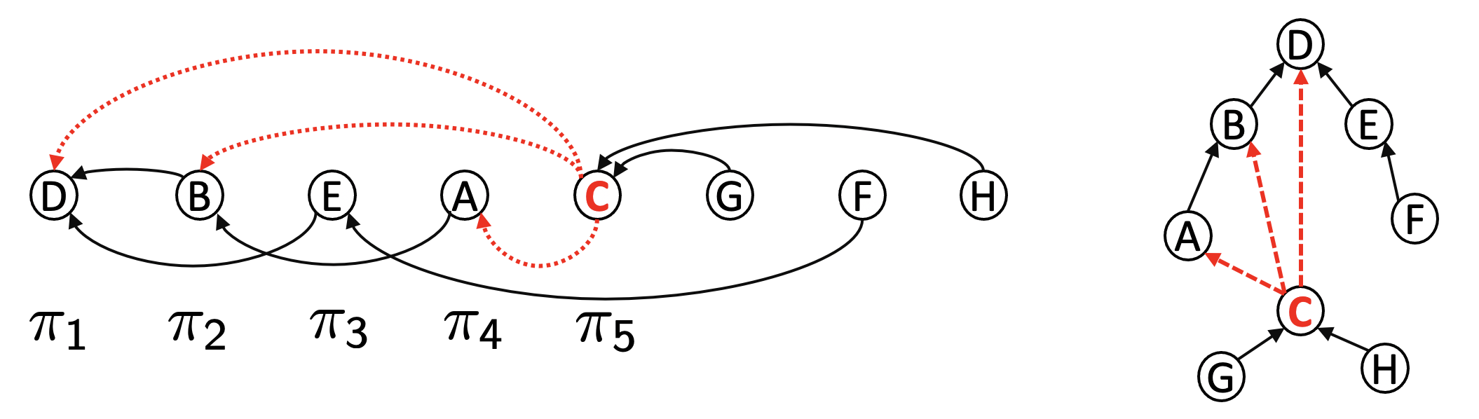
Figure 12: Sampling a parent for $\pi_{5}$ (node C).

At iteration $t$, to compute $Q_{\pi_{t}}(\cdot)$ with respect to $\pi_{t}$, for each node $v$ in the support of $Q_{\pi_{t}}(\cdot)$, we let $\tilde{\bm{f}}_{n}^{(v,\pi_{t})}$ denote the forest formed by removing the old edge $(\text{pa}(\pi_{t}),\pi_{t})$ and adding the new edge $(v,\pi_{t})$. We note that $v$ is allowed to be the old parent so that we may have $\tilde{\bm{f}}_{n}=\tilde{\bm{f}}_{n}^{(v,\pi_{t})}$. Then, for any $w_{t}$ in the support of $Q_{\pi_{t}}(\cdot)$, we have

$$Q_{\pi_{t}}(w_{t})=\frac{\mathbb{P}(\tilde{\bm{F}}_{n}=\tilde{\bm{f}}_{n}^{(w_{t},\pi_{t})}\,|\,\Pi=\pi,\tilde{\bm{G}}_{n}=\tilde{\bm{g}}_{n})}{\sum_{v}\mathbb{P}(\tilde{\bm{F}}_{n}=\tilde{\bm{f}}_{n}^{(v,\pi_{t})}\,|\,\Pi=\pi,\tilde{\bm{G}}_{n}=\tilde{\bm{g}}_{n})}.$$ (29)

In the PAPER models with Erdős–Rényi edges, We can compute the conditional distribution $\mathbb{P}(\tilde{\bm{F}}_{n}=\cdot\,|\,\Pi=\pi,\tilde{\bm{G}}_{n}=\tilde{\bm{g}}_{n})$ by using the fact that once when we condition on $\tilde{\bm{F}}_{n}=\tilde{\bm{f}}_{n}$, the remaining edges of $\tilde{\bm{G}}_{n}$ are uniformly random and the fact that $\Pi$ and $\bm{F}_{n}$ are independent. Thus,

$$\mathbb{P}(\tilde{\bm{F}}_{n}=\tilde{\bm{f}}_{n}\,|\,\Pi=\pi,\tilde{\bm{G}}_{n}=\tilde{\bm{g}}_{n})$$

$$\qquad\propto\mathbb{P}(\tilde{\bm{G}}_{n}=\tilde{\bm{g}}_{n}\,|\,\tilde{\bm{F}}_{n}=\tilde{\bm{f}}_{n},\Pi=\pi)\mathbb{P}(\tilde{\bm{F}}_{n}=\tilde{\bm{f}}_{n}\,|\,\Pi=\pi)$$

$$\qquad=\binom{\binom{n}{2}-(n-K(\tilde{\bm{f}}_{n}))}{m-(n-K(\tilde{\bm{f}}_{n}))}^{-1}\mathbb{P}(\bm{F}_{n}=\pi^{-1}\tilde{\bm{f}}_{n})\mathbbm{1}\{\tilde{\bm{f}}_{n}\in\mathcal{F}(\tilde{\bm{g}}_{n})\}$$

$$\qquad\propto\biggl{\{}\prod_{k=1}^{K(\tilde{\bm{f}}_{n})}\frac{n(n-1)/2-n+k)}{m-n+k}\biggr{\}}\mathbb{P}(\bm{F}_{n}=\pi^{-1}\tilde{\bm{f}}_{n})\mathbbm{1}\{\tilde{\bm{f}}_{n}\in\mathcal{F}(\tilde{\bm{g}}_{n})\}.$$ (30)

We now discuss the sampling procedure in detail in all the settings.

Single root setting: In the single root setting, we again use the notation $\tilde{\bm{t}}_{n}=\tilde{\bm{f}}_{n}$ to be consistent with Definition 1. The first term of (30) is a constant since $K(\tilde{\bm{t}}_{n})=1$ and may thus be ignored. Using the likelihood of APA trees (see Remark 2 as well as Proposition S1 from the Appendix) and using the fact that $\mathbb{P}(\bm{T}_{n}=\pi^{-1}\tilde{\bm{t}}_{n})>0$ when $\pi\in\text{hist}(\tilde{\bm{t}}_{n})$, we have that, for any $w_{t}\in\pi_{1:(t-1)}\cap N_{\tilde{\bm{g}}_{n}}(\pi_{t})$,

$$Q_{\pi_{t}}(w_{t})=\frac{\beta D_{\tilde{\bm{t}}^{(\cdot,\pi_{t})}_{n}}(w_{t})+\alpha}{\sum_{v\in\pi_{1:(t-1)}\cap N_{\tilde{\bm{g}}_{n}}(\pi_{t})}\beta D_{\tilde{\bm{t}}^{(\cdot,\pi_{t})}_{n}}(v)+\alpha},$$

where $\tilde{\bm{t}}^{(\cdot,\pi_{t})}_{n}$ is the disconnected graph obtained by removing the old edge $(\text{pa}(\pi_{t}),\pi_{t})$ from $\tilde{\bm{t}}_{n}$. We summarize the resulting procedure in Algorithm 2. Since we visit every node once and, for a single node $u$, it takes time $O(D_{\tilde{\bm{g}}_{n}}(u))$ to generate a new parent, the overall runtime of the second stage of the algorithm is $O(m)$. The computational complexity is the same under the fixed $K$ setting and the random $K$ setting.

Fixed $K>1$ setting: Since the number of trees $K$ is fixed, the first term of (30) is again a constant. Using likelihood of APA trees again (see Proposition S2 from the Appendix), we have that for any $w_{t}\in\pi_{1:(t-1)}\cap N_{\tilde{\bm{g}}_{n}}(\pi_{t})$,

$$Q_{\pi_{t}}(w_{t})=\frac{\beta D_{\tilde{\bm{f}}_{n}^{(\cdot,\pi_{t})}}(w_{t})+2\beta\mathbbm{1}\{w_{t}\in\pi_{1:K}\}+\alpha}{\sum_{v\in\pi_{1:(t-1)}\cap N_{\tilde{\bm{g}}_{n}}(\pi_{t})}\beta D_{\tilde{\bm{f}}_{n}^{(\cdot,\pi_{t})}}(v)+2\beta\mathbbm{1}\{v\in\pi_{1:K}\}+\alpha},$$

where, as with the single root setting, $\tilde{\bm{f}}_{n}^{(\cdot,\pi_{t})}$ is the forest obtained by removing the old edge $(\text{pa}(\pi_{t}),\pi_{t})$ from $\tilde{\bm{f}}_{n}$. The only difference from the single root setting is that we have a higher probability to attach to a root node because of the imaginary self-loop edge. We summarize the procedure in Algorithm 2.

Algorithm 2 Generating spanning forest $\tilde{\bm{f}}_{n}$ of $\tilde{\bm{g}}_{n}$ under either $\text{PAPER}(\alpha,\beta,\theta)$ or $\text{PAPER}(\alpha,\beta,K,\theta)$

Input: Graph $\tilde{\bm{g}}_{n}$, ordering $\pi\in\text{Bi}([n],\mathcal{U}_{n})$, and a spanning forest $\tilde{\bm{f}}_{n}$ with $K$ component trees.
Effect: Modifies $\tilde{\bm{f}}_{n}$ in place.

1:for $t=K+1,\ldots,n$ do:

2:     Remove old edge $(\pi_{t},pa(\pi_{t}))$ from $\tilde{\bm{f}}_{n}$ to obtain $\tilde{\bm{f}}_{n}^{(\cdot,\pi_{t})}$.

3:     Choose a node $w_{t}\in\pi_{1:(t-1)}\cap N_{\tilde{\bm{g}}_{n}}(\pi_{t})$ with probability proportional to

$$\left\{\begin{array}[]{cc}\beta D_{\tilde{\bm{f}}^{(\cdot,\pi_{t})}_{n}}(w_{t})+\alpha&\text{ under $\text{PAPER}(\alpha,\beta,\theta)$}\\ \beta D_{\tilde{\bm{f}}^{(\cdot,\pi_{t})}_{n}}(w)+2\beta\mathbbm{1}\{w\in\pi_{1:K}\}+\alpha&\text{ under $\text{PAPER}(\alpha,\beta,K,\theta)$}\end{array}\right.$$

4:     Add new edge $(\pi_{t},w_{t})$ to $\tilde{\bm{f}}_{n}$.

5:end for

Random $K$ roots setting: Under the $\text{PAPER}(\alpha,\beta,\alpha_{0},\theta)$ model, a node may become a new root in the sampling process and thus we must take into account the first term of (30). Moreover, in this setting, $Q_{\pi_{t}}(\cdot)$ for node $\pi_{t}$ is supported on $\{\emptyset\}\cup\bigl{(}\pi_{1:(t-1)}\cap N_{\tilde{\bm{g}}_{n}}(\pi_{t})\bigr{)}$ since we may turn the node $\pi_{t}$ into a new root node, in which case we set its parent to $\emptyset$ by convention. Define $\tilde{\alpha}_{0}:=\alpha_{0}\frac{m-n+K+\mathbbm{1}\{\pi_{t}\notin\tilde{s}\}}{n(n-1)/2-n+K+\mathbbm{1}\{\pi_{t}\notin\tilde{s}\}}$; we then have that, by Proposition S3, for any $w_{t}\in\{\emptyset\}\cup\bigl{(}\pi_{1:(t-1)}\cap N_{\tilde{\bm{g}}_{n}}(\pi_{t})\bigr{)}$,

$$Q_{\pi_{t}}(w_{t}) =\frac{\tilde{\alpha}_{0}}{\tilde{\alpha}_{0}+\sum_{v\in\pi_{1:(t-1)}\cap N_{\tilde{\bm{g}}_{n}}(\pi_{t})}\beta D_{\tilde{\bm{f}}^{(\cdot,\pi_{t})}_{n}}(v)+2\beta\mathbbm{1}\{v\in\tilde{s}\}+\alpha}\quad\text{ if $w_{t}=\emptyset$}$$

$$\textrm{and }Q_{\pi_{t}}(w_{t}) =\frac{\beta D_{\tilde{\bm{f}}_{n}^{(\cdot,\pi_{t})}}(w_{t})+2\beta\mathbbm{1}\{w_{t}\in S\}+\alpha}{\tilde{\alpha}_{0}+\sum_{v\in\pi_{1:(t-1)}\cap N_{\tilde{\bm{g}}_{n}}(\pi_{t})}\beta D_{\tilde{\bm{f}}_{n}^{(\cdot,\pi_{t})}}(v)+2\beta\mathbbm{1}\{v\in\tilde{s}\}+\alpha}\quad\text{ if $w_{t}\neq\emptyset$},$$

where, if $\pi_{t}$ is not a root node, $\tilde{\bm{f}}_{n}^{(\cdot,\pi_{t})}$ is the forest obtained by removing the old edge $(\pi_{t},\textbf{pa}(\pi_{t}))$ and if $\pi_{t}$ is a root node, then $\tilde{\bm{f}}_{n}^{(\cdot,\pi_{t})}=\tilde{\bm{f}}_{n}$. We summarize the resulting procedure in Algorithm 3.

Algorithm 3 Generating spanning forest $\tilde{\bm{f}}_{n}$ of $\tilde{\bm{g}}_{n}$ under $\text{PAPER}(\alpha,\beta,\alpha_{0},\theta)$

Input: Graph $\tilde{\bm{g}}_{n}$, ordering $\pi\in\text{Bi}([n],\mathcal{U}_{n})$, and a spanning forest $\tilde{\bm{f}}_{n}$.
Effect: Modifies $\tilde{\bm{f}}_{n}$ in place.

1:Let $\tilde{s}$ be the set of root nodes.

2:for $t=2,3,\ldots,n$ do:

3:     If $\pi_{t}\notin\tilde{s}$, remove edge $(\pi_{t},pa(\pi_{t}))$ from $\tilde{\bm{f}}_{n}$ to get $\tilde{\bm{f}}^{(\cdot,\pi_{t})}_{n}$. Else, let $\tilde{s}=\tilde{s}\backslash\{w_{t}\}$ and let $\tilde{\bm{f}}^{(\cdot,\pi_{t})}_{n}=\tilde{\bm{f}}_{n}$.

4:     Choose a node $w_{t}\in\{\emptyset\}\cup\bigl{(}\pi_{1:(t-1)}\cap N_{\tilde{\bm{g}}_{n}}(\pi_{t})\bigr{)}$ with probability proportional to

$$\left\{\begin{array}[]{cc}\alpha_{0}&\text{ for $w_{t}=\emptyset$}\\ \beta D_{\tilde{\bm{f}}^{(\cdot,\pi_{t})}_{n}}(w_{t})+2\beta\mathbbm{1}\{w_{t}\in\tilde{s}\}+\alpha&\text{ for $w_{t}\neq\emptyset$}\end{array}\right.$$

5:     If $w_{t}\neq\emptyset$, let $\tilde{\bm{f}}_{n}=\tilde{\bm{f}}_{n}^{(\cdot,\pi_{t})}\cup(\pi_{t},w_{t})$. Otherwise, let $\tilde{s}=\tilde{s}\cup\{\pi_{t}\}$ and $\tilde{\bm{f}}_{n}=\tilde{\bm{f}}^{(\cdot,\pi_{t})}_{n}$.

6:end for

Sequential noise setting: Under the seq-PAPER setting, we use the same sampling procedure but the sampling probabilities become more complicated. From (29), we see that, for $w\in N_{\tilde{\bm{g}}_{n}}\cap\pi_{1:(t-1)}$,

$$Q_{\pi_{t}}(w) \propto\mathbb{P}(\tilde{\bm{T}}_{n}=\tilde{\bm{t}}_{n}^{(w,\pi_{t})}\,|\,\Pi=\pi,\tilde{\bm{G}}_{n}=\tilde{\bm{g}}_{n})$$

$$\propto\underbrace{\mathbb{P}(\tilde{\bm{G}}_{n}=\tilde{\bm{g}}_{n}\,|\,\tilde{\bm{T}}_{n}=\tilde{\bm{t}}_{n}^{(w,\pi_{t})},\Pi=\pi)}_{\text{noise term}}\mathbb{P}(\tilde{\bm{T}}_{n}=\tilde{\bm{t}}_{n}^{(w,\pi_{t})}\,|\,\Pi=\pi).$$

Under the seq-PAPER model, the noise term also depends on $w$ since choosing a new parent for $\pi_{t}$ would change the tree degrees of some of the nodes. Naively computing $Q_{\pi_{t}}(w)$ takes time $O(n)$, but in Section S3.5.3 of the Appendix (using results from Section S3.5.1), we give a detailed algorithm to compute $Q_{\pi_{t}}(w)$ in time $O(D_{\tilde{\bm{g}}_{n}}(w))$ so that overall, we can sample a new parent for $\pi_{t}$ in time proportional to the number of neighbors of neighbors of $\pi_{t}$.

When we have deletion noise, as the case of the $\text{seq-PAPER}^{*}$ model, the latent tree $\tilde{\bm{T}}_{n}$ need not be a subgraph of $\tilde{\bm{G}}_{n}$ and hence, when sampling a new parent for $\pi_{t}$, we must consider all of $\pi_{1:(t-1)}$ and not just graph neighbors of $\pi_{t}$. Thus, we draw $w\in\pi_{1:(t-1)}$ with probability $Q_{\pi_{t}}(w)$ and set $\text{pa}(\pi_{t})=w$. We give the detailed algorithm for computing $Q_{\pi_{t}}(w)$ in Section S3.5.3 of the Appendix.

4.3 Other aspects of the algorithm

Parameter estimation: To estimate $\alpha$ and $\beta$, we derive an EM algorithm in Section S3.1 of the Appendix. The noise level $\theta$ is easy to estimate via $\hat{\theta}=\frac{m-(n-1)}{n(n-1)/2-(n-1)}$ in the single root setting. The inference algorithm in fact does not require knowledge of $\theta$ since it conditions on the number of edges $m$ of the observed graph. We discuss some ways to select the number of trees $K$ in the fixed $K$ root setting and ways to estimate $\alpha_{0}$ in the random $K$ roots setting in Section S3.4 of the Appendix.

Inference from posterior samples: The Gibbs sampler described in Section 4.1 and Section 4.2 generates a Monte Carlo sequence $\{(\pi^{(j)},\tilde{\bm{f}}_{n}^{(j)})\}_{j=1}^{J}$ where $J$ is the number of Monte Carlo samples. A straightforward way to approximate the posterior root probability is to use the empirical distribution based on all the $\pi^{(j)}$’s. However, we can construct a much more accurate approximation by taking advantage of the fact that the posterior root probability is easy to compute on a tree.

Consider the single root setting for simplicity where the posterior root probability is $\mathbb{P}(\Pi_{1}=u\,|\,\tilde{\bm{G}}_{n}=\tilde{\bm{g}}_{n})$ for any node $u$. In this case, we may compute distributions $Q^{(1)},Q^{(2)},\ldots,Q^{(J)}$ over the nodes by

$$Q^{(j)} =\mathbb{P}(\Pi_{1}=u\,|\,\tilde{\bm{T}}_{n}=\tilde{\bm{t}}_{n}^{(j)},\tilde{\bm{G}}_{n}=\tilde{\bm{g}}_{n})=\mathbb{P}(\Pi_{1}=u\,|\,\tilde{\bm{T}}_{n}=\tilde{\bm{t}}_{n}^{(j)})=\frac{h(u,\tilde{\bm{t}}_{n}^{(j)})}{h(\tilde{\bm{t}}_{n}^{(j)})}.$$

Then, we output $\frac{1}{J}\sum_{j=1}^{J}Q^{(j)}$ as our approximation of the posterior root distribution. In the multiple roots setting, we use the same procedure except that we compute $u\mapsto\mathbb{P}(u\in\tilde{S}\,|\,\tilde{\bm{F}}_{n}=\tilde{\bm{f}}_{n}^{(j)})$ and then average across $j\in\{1,2,\ldots,J\}$.

In the multiple roots setting, each Monte Carlo sample of the forest $\tilde{\bm{f}}_{n}^{(j)}$ contain either $K$ disjoint trees in the fixed $K$ setting or a random number of disjoint trees in the random $K$ setting. These disjoint trees provide a posterior sample of the communities on the network and using them, we may estimate the community structure of the network. We provide details on one way of using posterior samples for community recovery in Section 6.3 and 6.4.

The Gibbs sampling algorithm scales to large networks. We are able to run it on networks of up to a million nodes (c.f. Section 6.2.2) on a single 2020 MacBook Pro laptop. To give a rough sense of the runtime, it takes about 1 second to perform one outer loop of the Gibbs sampler on a graph of 10,000 nodes and 20,000 edges. In Section S3.4 of the appendix, we provide more details on practical usage of the Gibbs sampler such as convergence criterion.

Initialization: In the single root setting, to initialize the Gibbs sampling algorithm, we recommend generating the initial tree $\tilde{\bm{t}}_{n}$ uniformly at random from the set of spanning trees $\mathcal{T}(\tilde{\bm{g}}_{n})$ of the observed graph, which can be efficiently done via elegant random-walk-based algorithms such as the Aldous–Broder algorithm (Broder, 1989; Aldous, 1990) or Wilson’s algorithm (Wilson, 1996). We then initialize $\pi$ by drawing an ordering uniformly from the history of the initial tree. This initialization distribution is guaranteed to be overdispersed and works very well in practice. The same initialization works for the random $K$ setting. For the fixed $K$ setting, we can form the initial forest by constructing uniformly random spanning tree $\tilde{\bm{t}}_{n}$ and uniformly random ordering $\pi$ as usual, taking the first $K$ nodes of the $\pi$ as the root nodes, and removing all tree edges between them to obtain an initial $\tilde{\bm{f}}_{n}$. We use Wilson’s algorithm in our implementation.

5 Theoretical Analysis

We provide theoretical support for our approach by deriving bounds on the size of our proposed confidence sets when the observed graph has the PAPER distribution. In particular, we aim to quantify how the quality of inference deterioriates with the noise level $\theta$, that is, how the size of the confidence set increases with $\theta$. For simplicity, for consider only the single root setting and we do not take into account approximation errors introduced by the Gibbs sampler, that is, we analyze the confidence set constructed from the exact posterior root probabilities.

We begin with a type of optimality statement which shows that the size of the confidence set $B_{\epsilon}(\cdot)$, as defined in (8), is of no larger order than any other asymptotically valid confidence set. Intuitively, this is because $B_{\epsilon}(\cdot)$ can be interpreted as a “Bayes estimator” for the root node.

Lemma 10.

Let $\epsilon$ be in $(0,1)$, let $\bm{G}_{n}\sim\text{PAPER}(\alpha,\beta,\theta)$, and let $\bm{G}^{*}_{n}=\rho\bm{G}_{n}$ be the observed alphabetically labeled graph for some $\rho\in\text{Bi}([n],\mathcal{U}_{n})$. Let $B_{\epsilon}(\mathbf{G}^{*}_{n})$ be defined as in (7) and (8). Fix any $\delta\in(0,1)$ and let $C_{\delta\epsilon}(\mathbf{G}_{n}^{*})$ be any confidence set for the root node that is labeling-equivariant and has asymptotic coverage level $1-\delta\epsilon$, that is, $\limsup_{n\rightarrow\infty}\mathbb{P}(\rho_{1}\notin C_{\delta\epsilon}(\mathbf{G}^{*}_{n}))\leq\delta\epsilon$. Then, we have that

$$\limsup_{n\rightarrow\infty}\mathbb{P}\bigl{(}|B_{\epsilon}(\mathbf{G}_{n}^{*})|\geq|C_{\delta\epsilon}(\mathbf{G}_{n}^{*})|\bigr{)}\leq\delta.$$

We provide the proof of Lemma 10 in Section S4 of the appendix.

Ideally, we would compare the size of $B_{\epsilon}(\cdot)$ with $C_{\epsilon}(\cdot)$ at the same level. It is however much easier to compare with the more conservative $C_{\delta\epsilon}(\cdot)$. In many cases, the size of a confidence set $|C_{\epsilon}(\cdot)|$ has bounds of the form $f(n)g(\epsilon^{-1})$ for some functions $f$ and $g$ (see e.g. Banerjee and Bhamidi (2020)) so that comparing with $C_{\delta\epsilon}(\cdot)$ adds only a multiplicative constant to the bound.

Lemma 10 is useful because it is difficult to directly bound the confidence set $B_{\epsilon}(\cdot)$ as a function of $n$ and the parameters; Lemma 10 shows that we can indirectly upper bound it by analyzing a simpler asymptotically valid confidence set. Our strategy then is to construct confidence sets based on the degree of the nodes whose size is much easier to bound through well-understood probabilistic properties of preferential attachment trees. This leads to our next result which provides explicit bounds on the size of the confidence set $B_{\epsilon}(\cdot)$ when the underlying tree is LPA.

Theorem 11.

Let $\bm{G}_{n}\sim\text{PAPER}(\alpha,\beta,\theta)$ for $\beta=1$, $\alpha=0$, and $\theta\in[0,1]$. For $t\in[n]$, let $D_{\bm{G}_{n}}(t)$ be the degree of node with arrival time $t$ and for $k\in[n]$, let $k\mathchar 45\relax\max(D_{\bm{G}_{n}})$ be the $k$-th largest degree of $\bm{G}_{n}$. Let $\delta>0$ be arbitrary and suppose $\theta\leq n^{-\frac{1}{2}-\delta}$. Then, for any $\epsilon>0$, there exists $L_{\epsilon}\in\mathbb{N}$ (dependent on $\delta$ but not on $n$) such that

$$\limsup_{n\rightarrow\infty}\mathbb{P}\bigl{\{}D_{\bm{G}_{n}}(1)\leq L_{\epsilon}\mathchar 45\relax\max(D_{\bm{G}_{n}})\bigr{\}}\leq\epsilon.$$ (31)

As a direct consequence, if $\theta=O(n^{-\frac{1}{2}-\delta})$ for any $\delta>0$, then, for any $\epsilon\in(0,1)$,

$$|B_{\epsilon}(\bm{G}^{*}_{n})|=O_{p}(1).$$

We relegate the proof of Theorem 11 in Section S4.1 of the appendix and provide a short sketch here: we use results from Peköz et al. (2014) which show that the degree sequence of an LPA tree, when normalized by $\frac{1}{\sqrt{n}}$, converges to a limiting distribution in the $\ell_{q}$ sequential metric sense, which shows that (31) holds for the tree degree $D_{\bm{T}_{n}}(\cdot)$, that is, the degree of the root node is one of the highest among all the nodes. Since $D_{\bm{G}_{n}}=D_{\bm{T}_{n}}+D_{\bm{R}_{n}}$, we show that if the noise level $\theta$ is less than $n^{-1/2-\delta}$ for some $\delta>0$, then the degree of the noisy edges $D_{\bm{R}_{n}}$ has a second order effect and (31) remains valid.

We know from existing results (such as Bubeck, Devroye and Lugosi (2017, Theorem 6); see also Crane and Xu (2021, Corollary 7)) that $|B_{\epsilon}(\bm{T}_{n}^{*})|$ is $O_{p}(1)$ in the $\theta=0$ case where we observe the LPA tree $\bm{T}_{n}^{*}$. Theorem 11 shows that this phenomenon is quite robust to noise. Indeed, when $\theta=n^{-1/2-\delta}$, the observed graph would have approximately $n^{3/2-\delta}$ noisy edges and only $n-1$ tree edges.

The situation is different when the underlying latent tree has the UA distribution, where $\alpha=1$ and $\beta=0$. In this case, we have the following result:

Theorem 12.

Let $\bm{G}_{n}\sim\text{PAPER}(\alpha,\beta,\theta)$ for $\alpha=1$, $\beta=0$, and $\theta\in[0,1]$. For $t\in[n]$, let $D_{\bm{G}_{n}}(t)$ be the degree of node with arrival time $t$ and for $k\in[n]$, let $k\mathchar 45\relax\max(D_{\bm{G}_{n}})$ be the $k$-th largest degree of $\bm{G}_{n}$. Suppose $\theta=o\bigl{(}\frac{\log n}{n}\bigr{)}$ and let $\epsilon\in(0,1)$ be arbitrary. For any $\eta\in(0,1)$, define $L_{\eta,n,\epsilon}:=n^{\eta}+\epsilon^{-1}n^{1-(2-\eta)h\bigl{(}\frac{\eta}{2-\eta}\bigr{)}}$ where $h(x)=(1+x)\log(1+x)-x$ for $x\geq 0$. Then, we have that

$$\limsup_{n\rightarrow\infty}\mathbb{P}\bigl{\{}D_{\bm{G}_{n}}(1)\leq L_{\eta,n,\epsilon}\mathchar 45\relax\max(D_{\bm{G}_{n}})\bigr{\}}\leq\epsilon.$$ (32)

As a direct consequence, if $\theta=o(\frac{\log n}{n})$, then, for some $\gamma\leq 0.8$, we have that

$$n^{-\gamma}\epsilon^{-1}|B_{\epsilon}(\bm{G}^{*}_{n})|=O_{p}(1)\,\quad\text{for any $\epsilon\in(0,1)$}.$$

We relegate the proof of Theorem 12 to Section S4.2 of the appendix. The proof technique is similar to that of Theorem 11 except that we use concentration inequalities to derive (32).

Comparing Theorem 12 with Theorem 11, we see two important differences. First, even if the noise level is small, we can no longer guarantee that $|B_{\epsilon}(\bm{G}_{n}^{*})|$ is bounded even as $n$ increases. Instead, we have the much weaker bound that $|B_{\epsilon}(\bm{G}^{*}_{n})|$ is less than $O(n^{\gamma})$ for some $\gamma<0.8$. We believe this bound is not tight; we observe from simulations in Section 6.1 (see Figure 13) that the size of the confidence set $B_{\epsilon}(\cdot)$ is indeed $O_{p}(1)$ even when the noise level is of order $\frac{\log n}{n}$. The bound is sub-optimal because the degree of the nodes is not informative of their latent ordering when the latent tree has the UA distribution; hence, $B_{\epsilon}(\cdot)$ could be much smaller than confidence sets constructed solely from degree information. Intuitively, this is because largest degree nodes do not persist in uniform attachment as opposed to linear preferential attachment (Dereich and Mörters, 2009; Galashin, 2013).

The second difference is that the noise tolerance is much smaller. We require $\theta$ to be smaller than $\frac{\log n}{n}$ rather than $n^{-1/2}$. We conjecture that these rates are tight in the following sense:

Conjecture 13.

Let $\bm{G}_{n}\sim\text{PAPER}(\alpha,\beta,\theta)$ for $\alpha=1$, $\beta=0$, and $\theta\in[0,1]$.

1. Suppose $\alpha=0$ and $\beta=1$ (LPA). If $\theta=o(n^{-1/2})$, then $|B_{\epsilon}(\bm{G}^{*}_{n})|=O_{p}(1)$ and if $\theta=\omega(n^{-1/2})$, then every asymptotically valid confidence set has size that diverges with $n$.

2. Suppose $\alpha=1$ and $\beta=0$ (UA). If $\theta=o(\frac{\log n}{n})$, then $|B_{\epsilon}(\bm{G}^{*}_{n})|=O_{p}(1)$ and if $\theta=\omega(\frac{\log n}{n})$, then every asymptotically valid confidence set has size that diverges with $n$.

We provide empirical support for this conjecture in Section 6.1, particularly Figure 13. In those experiments, we see that, when the latent tree has the LPA distribution and when $\theta=cn^{-1/2}$ where $c>0$ is small, the size of $B_{\epsilon}$ does not increase with $n$; however, when $c$ (and hence $\theta$) is large, $B_{\epsilon}$ is larger when the size of the graph $n$ is larger. The same phenomenon holds when the latent tree has the UA distribution when $\theta=c\frac{\log n}{n}$.

6 Empirical Studies

We have implemented the inference approach in Section 3 and the sampling algorithm in Section 4 in a Python package named paper-network, which can be installed via command line pip install paper-network on the terminal and then imported in Python via import PAPER. The source code of the package, along with examples and documentation, are available at the website https://github.com/nineisprime/PAPER. All the code used in this Section are also available there under the directory paperexp. We also give detailed sampler diagnostics information in Section S5.4 of the Appendix.

6.1 Simulation

Frequentist coverage in the single root setting: In our first simulation study, we empirically verify Theorem 7 by showing that a level $1-\epsilon$ credible set for the root node constructed from the posterior root probabilities has frequentist coverage at exactly the same level $1-\epsilon$. We consider three different settings of parameters: $\alpha=0,\beta=1$ (LPA), $\alpha=1,\beta=0$ (UA), and $\alpha=8,\beta=1$. We generate $\bm{G}_{n}^{*}$ according to the $\text{PAPER}(\alpha,\beta,\theta)$ model with $n=3,000$ nodes and $m=7,500$ edges. We then estimate $\alpha$ and $\beta$ using the method given in Section S3.1, compute the level $\epsilon\in\{0.2,0.05,0.01\}$ credible sets, and record whether they cover the true root node. We repeat the experiment over 300 independent trials and report the results in Table 2. We observe that the credible sets attain the nominal coverage and that the size of the credile sets are small compared to the number of nodes $n$.

$(\alpha,\beta)$	(0, 1)	(1, 0)	(8, 1)	(0, 1)	(1, 0)	(8, 1)	(0, 1)	(1, 0)
Theoretical coverage	0.8	0.8	0.8	0.95	0.95	0.95	0.99	0.99
Empirical coverage	0.8	0.823	0.82	0.937	0.943	0.94	0.983	0.993
Ave. conf. set size	7	12	9	42	42	31	183	115

Table 2: Empirical coverage of our confidence set for the root node. We report the average over 300 trials. Graph has $n=3000$ nodes and $m=7,500$ edges in all cases.

Size of the confidence set: In our second simulation study, we study the effect of the sample size $n$ and the magnitude of the noisy edge probability $\theta$ on the size of the confidence set. We let $\bm{G}^{*}_{n}$ be the observed graph with $n$ nodes and $m$ edges according to the $\text{PAPER}(\alpha,\beta,\theta)$ model where we consider $(\alpha,\beta)=(0,1)$ (LPA) or $(1,0)$ (UA). Since a tree with $n$ nodes always contains $n-1$ edges, $\frac{n^{2}}{2}\theta+n$ is approximately equal to the number of edges $m$ in the observed graph $\bm{G}_{n}^{*}$.

We empirically show that the confidence set size does not depend on $n$ so long as $\theta$ is much smaller than $n^{-1/2}$ for LPA and much smaller than $\frac{\log n}{n}$ for UA. To that end, we set $m=cn\sqrt{n}$ for $c\in\{0.1,0.2,0.4,0.6,0.8,1\}$ for LPA and $m=cn\log n$ for $c\in\{0.15,0.2,0.4,0.6,0.8\}$ for UA. We then plot the average size of the confidence set with respect to $c$ for $n\in\{5000,10000\}$. We plot the curve for $n=5,000$ and for $n=10,000$ on the same figure and observe that, when $c$ is small, the two curves overlap completely but when $c$ is large, the $n=10,000$ curve lies above the $n=5,000$ curve. This provides empirical support to Theorem 11 and Theorem 12. In fact, this experiment shows that the bound of $n^{\gamma}$ on the size of the confidence set in Theorem 12 is loose; the actual size does not increase with $n$. The fact that the confidence set size seems to diverge with $n$ when $c$ is larger supports Conjecture 13 and suggests that the problem of root inference exhibits a phase transition when $\theta\approx\frac{1}{\sqrt{n}}$ under the LPA model and $\theta\approx\frac{\log n}{n}$ under the UA model.

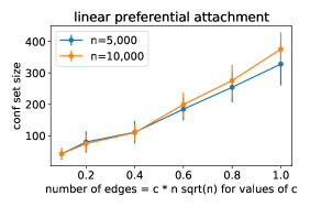
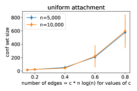
Figure 13: Size of the confidence set vs. the number of edges.

Frequentist coverage under sequential noise models: In our third simulation study, we verify Theorem 7 for the seq-PAPER model with sequential noise described in Section 2.3. We generate $\bm{G}_{n}^{*}$ according to both the $\text{seq-PAPER}(\alpha,\beta,\theta,\tilde{\alpha},\tilde{\beta})$ model and the $\text{seq-PAPER}^{*}(\alpha,\beta,\theta,\tilde{\alpha},\tilde{\beta},\eta)$ model with deletion noise. We then construct the credible sets for the root node from posterior root probabilities computed via the algorithm given in Section 4. We repeat the experiment over 200 independent trials and report the results in Tables 3 and 4. We observe that the credible sets attain the nominal coverage. We also note that Table 4 shows that the $\text{seq-PAPER}^{*}$ model can tolerate tree deletion probability up to $\eta=0.08$ without significant increase in the confidence set sizes.

$(\alpha,\beta)$ (with $\tilde{\alpha}=\alpha$, $\tilde{\beta}=\beta$)	(0, 1)	(1, 0)	(0, 1)	(1, 0)	(0, 1)	(1, 0)
Theoretical coverage	0.8	0.8	0.95	0.95	0.99	0.99
Empirical coverage	0.795	0.895	0.935	0.965	0.970	0.995
Ave. conf. set size	7	7	25	16	56	28

Table 3: Empirical coverage of our confidence set for the $\text{seq-PAPER}(\alpha,\beta,\theta,\tilde{\alpha},\tilde{\beta})$ model without deletion noise, with $\theta=1.5$ and $\tilde{\alpha}=\alpha$ and $\tilde{\beta}=\beta$. We report the average over 200 trials. Graph has $n=600$ nodes and around $m\approx 1500$ edges in all cases.

$\eta$ (tree edge deletion probability)	0	0	0.04	0.04	0.08	0.08
Theoretical coverage	0.8	0.95	0.8	0.95	0.8	0.95
Empirical coverage	0.825	0.96	0.84	0.95	0.85	0.98
Ave. conf. set size	5.9	14.1	6.3	15.0	6.7	15.9

Table 4: Empirical coverage of our confidence set for the $\text{seq-PAPER}^{*}(\alpha,\beta,\theta,\tilde{\alpha},\tilde{\beta},\eta)$ model with deletion noise, with $\alpha=0,\beta=1,\tilde{\alpha}=8,\tilde{\beta}=1,\theta=1.5$ in all cases. We report the average over 200 trials. Graph has $n=300$ nodes and around $m\approx 750$ edges in all cases.

Frequentist coverage for multiple roots: Our next simulation study is similar to the first except that we generate graphs from the $\text{PAPER}(\alpha,\beta,K,\theta)$ model with $K=2$. We construct our credible sets as described in Section 3.3 and verify Theorem 8 by showing that the credible set at level $1-\epsilon$ also has frequentist coverage at exactly the same level. We consider two different settings of parameters: $\alpha=0,\beta=1$ (LPA) and $\alpha=1,\beta=0$ (UA). We generate $\bm{G}_{n}^{*}$ according to the $\text{PAPER}(\alpha,\beta,K,\theta)$ model with $n=700$ nodes, $m=1,000$ edges, and $K=2$. We then estimate $\alpha$ and $\beta$ using the method given in Section S3.1, compute the level $\epsilon\in\{0.2,0.05,0.01\}$ credible sets, and record whether they contain the true set of root nodes. We repeat the experiment over 200 independent trials and report the results in Table 5. We observe that the credible sets attain the nominal coverage. In the LPA setting, the size of the credible sets are small but in the UA setting, the sizes of the credible sets become much larger. We relegate an in-depth analysis of this phenomenon to future work.

$(\alpha,\beta)$	(0, 1)	(1, 0)	(0, 1)	(1, 0)	(0, 1)	(1, 0)
Theoretical coverage	0.8	0.8	0.95	0.95	0.99	0.99
Empirical coverage	0.826	0.826	0.933	0.964	0.974	0.985
Ave. conf. set size	5	57	12	155	31	295

Table 5: Empirical coverage of our confidence set for the set of $K=2$ root nodes. We report the average over 200 trials. Graph has $n=700$ nodes and $m=1,000$ edges in all cases.

Posterior on $K$ in the random $K$ roots setting: In our last simulation experiment, we generate PAPER graphs with $K=2$ roots but perform posterior inference using the $\text{PAPER}(\alpha,\beta,\alpha_{0},\theta)$ model and study resulting posterior distribution over the number of roots $K$. We consider two different settings of parameters: $\alpha=0,\beta=1$ (LPA) and $\alpha=1,\beta=0$ (UA). We generate $\bm{G}_{n}^{*}$ according to the $\text{PAPER}(\alpha,\beta,K,\theta)$ model with $n=700$ nodes, $m=1,000$ edges, and $K=2$. We report the posterior distribution over $K$, averaged over 20 independent trials, in Figure 14. We observe that, in both cases, the mode of the posterior distribution over $K$ is 2, which is the true number of roots. However, the distributions exhibits high variance, which could be due to the fact that the two true latent trees may have significantly different sizes.

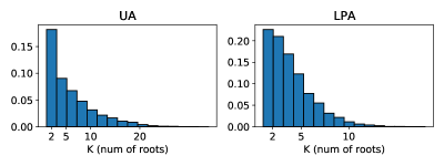
Figure 14: Posterior distribution over $K$ averaged across 20 independent trials. Left: networks have two latent UA trees. Right: networks have two latent LPA trees.

6.2 Single root analysis on real data

We now apply the single root PAPER model on real world networks. In a few cases (Section 6.2.1), we can ascertain from domain knowledge that the network originated from a single root node but more often, we use the single root model to identify important nodes and subgraphs (Section 6.2.2).

6.2.1 Flu transmission network

We analyze a person-to-person contact network among 32 students in a London classroom during a flu outbreak (Hens et al., 2012). We extract the data from Figure 3 in Hens et al. (2012) and illustrate the network in the left sub-figure of Figure 15. Public health investigation revealed that the outbreak originated from a single student, which is the true patient zero and shown as the orange node in Figure 15. We apply the PAPER model with a single root to this network. We estimate that $\beta=1$ and $\alpha=53.06$ using the method described in Section S3.1 and compute the $60\%,80\%,95\%$, and $99\%$ confidence sets. All the confidence sets contain the true patient zero and their sizes are as followed:

$$60\% 80\% 95\% 99\%$$: 6 nodes : 10 nodes : 19 nodes : 27 nodes.

We provide the approximate posterior root probabilities of the top 7 nodes in Figure 15. The true patient zero has a posterior root probability of $0.11$ is the node with the 3rd highest posterior root probability. In the center and right sub-figure of Figure 15, we also show two of the latent trees $\tilde{\bm{T}}_{n}$ that were generated by the Gibbs sampler.

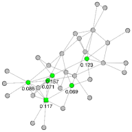
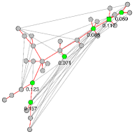
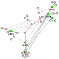
Figure 15: Left: contact network among 32 students in a flu outbreak. Center and right: two examples of the latent tree generated by the Gibbs sampler.

6.2.2 Visualizing central subgraphs

Large scale real graphs are difficult to visualize but one can often learn salient structural properties of a graph by visualizing a smaller subgraph that contains the most important nodes. In this section, we apply the single root PAPER model on four large networks and, for each graph, display the subgraph that comprises the 200 nodes with the highest posterior root probability. We see that the result reveals striking differences between the different graphs. Unfortunately, we do not have the node labels on any of these four graphs and can only make qualitative interpretations of the results.

MathSciNet collaboration network: We first consider a collaboration network of research publications from MathSciNet, which is publicly available in the Network Repository (Rossi and Ahmed, 2015) at the link http://networkrepository.com/ca-MathSciNet.php. This network has $n=332,689$ nodes and $m=820,644$ edges, with a maximum degree of $496$. Using the method described in Section S3.1, we estimate $\beta=1$ and $\alpha=0$. The sizes of confidence sets are:

$$60\% 80\% 95\% 99\%$$: 3 nodes : 6 nodes : 21 nodes : 112 nodes.

We display the subgraph containing the 200 nodes with the highest posterior root probability in Figure 16(a). We observe that the subgraph reveals a cluster structure that may represent the different academic disciplines.

University of Notre Dame website network: We study a network of hyperlinks between webpages of University of Notre Dame (Albert et al., 1999), which is publicly available at the website https://snap.stanford.edu/data/web-NotreDame.html. This network has $n=325,729$ nodes and $m=1,090,108$ edges, with a maximum degree of 10,721. Using the method described in Section S3.1, we estimate $\beta=1$ and $\alpha=0$. The sizes of confidence sets are:

$$\text{ $60\%$: 2 nodes }\quad\text{ $80\%$: 21 nodes }\quad\text{ $95\%$: 524 nodes }\quad\text{ $99\%$: 3498 nodes }.$$

We observe that the central subgraph (shown in Figure 16(b)) reveals two hub nodes with many sparsely connected “spokes”.

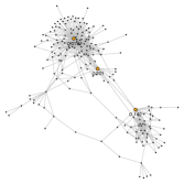
(a) MathSciNet subgraph

(b) Notre Dame subgraph

Figure 16: Subgraph of the 200 nodes with highest posterior root probabilities.

6.3 Community recovery with the fixed $K$ model

In this section, we show that we can use the PAPER model with multiple roots for community recovery on real world networks. To estimate the community membership from the posterior samples, we use a greedy matching procedure. To be precise, our Gibbs sampler outputs a sequence of forests $\tilde{\bm{f}}_{n}^{(1)},\ldots,\tilde{\bm{f}}_{n}^{(J)}$ where $J$ is the number of Monte Carlo samples. Each forest $\tilde{\bm{f}}_{n}^{(j)}$ contains $K$ component trees which we denote $\tilde{\bm{t}}^{(1,j)},\tilde{\bm{t}}^{(2,j)},\ldots,\tilde{\bm{t}}^{(K,j)}$. We write $Q_{k}^{(j)}(\cdot):=\mathbb{P}(\Pi_{1}=\cdot\,|\,\tilde{\bm{T}}=\tilde{\bm{t}}^{(k,j)})$ as the posterior root distribution of the $k$-th tree of the $j$-th Monte Carlo sample. Since the tree labels may switch from sample to sample, we use the following matching procedure: we maintain $K$ distributions $Q_{1}(\cdot),Q_{2}(\cdot),\ldots,Q_{K}(\cdot)$ and initially set $Q_{k}=Q_{k}^{(1)}$ for all $k\in[K]$. Then, for $j=2,3,\ldots,J$, we use the Hungarian algorithm to compute a one-to-one matching $\sigma\,:\,[K]\rightarrow[K]$ that minimizes the overall total variation distance

$$\sum_{k=1}^{K}\text{TV}(Q_{k}^{(j)},Q_{\sigma(k)}).$$

Once we compute the matching, we then update $Q_{\sigma(k)}\leftarrow\frac{j-1}{j}Q_{\sigma(k)}+\frac{1}{j}Q_{k}^{(j)}$.

In this way, we interpret $Q_{1},\ldots,Q_{K}$ as the average posterior root distributions for the $K$ trees across all the Monte Carlo samples and using the matching, we may also compute the posterior probability $\mathbb{P}(\text{ $u$ in tree $k$ }\,|\,\tilde{\bm{G}}_{n}=\tilde{\bm{g}}_{n})$, which allows us to perform community detection – we put node $u$ in cluster $k$ if $\mathbb{P}(\text{ $u$ in tree $k$ }\,|\,\tilde{\bm{G}}_{n}=\tilde{\bm{g}}_{n})\geq\mathbb{P}(\text{ $u$ in tree $k^{\prime}$ }\,|\,\tilde{\bm{G}}_{n}=\tilde{\bm{g}}_{n})$ for all $k^{\prime}\neq k$. We use the greedy matching procedure for computational efficiency – slower but more principles approaches are studied by e.g. Wade and Ghahramani (2018).

6.3.1 Karate club network

We apply the PAPER model to Zachary’s karate club network Zachary (1977), which is publicly available at http://www-personal.umich.edu/ mejn/netdata/. The karate club network has $n=34$ nodes and $m=76$ edges, where two individuals share an edge if they socialize with each other. The network has two ground truth communities, one led by the instructor and one led by the administrator (shown as rectangular nodes in Figure 17. These two communities later split into two separate clubs. In this case, we apply the PAPER model with $K=2$ roots. For every node $u$, we consider the community membership probability $\mathbb{P}(\text{$u$ in tree 1}\,|\,\tilde{\bm{G}}_{n})$ and assign $u$ to community $1$ if and only if this value is greater than $0.5$. We show the result in in Figure 17, where each node has a color that reflects its community membership probability.

We correctly cluster all but one node, which matches the performance of degree-corrected SBM Karrer and Newman (2011); Amini et al. (2013) (DCSBM)–the current the state of the art model for community detection. The node that we misclassify has a posterior probability $\mathbb{P}(\text{$u$ in tree 1}\,|\,\tilde{\bm{G}}_{n})=0.47$, indicating that the model is indeed unsure of whether it belong in community 1 or 2. We note that the PAPER model requires only 3 parameters whereas the DCSBM for this network requires 38 parameters because each node has a degree correction parameter. SBM without degree correction performs badly Karrer and Newman (2011).

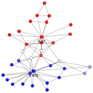
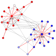
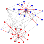
Figure 17: Left: karate club network where node color reflects community membership probability. Center and right: two examples of the latent forest generated by the Gibbs sampler.

6.3.2 Political blogs network

Next, we analyze a political blogs network (Adamic and Glance, 2005) that is frequently used as a benchmark for network clustering algorithms; the full network is publicly available at the website http://www-personal.umich.edu/ mejn/netdata/. This network contains $m=16,714$ edges between $n=1,222$ blogs, where two blogs are connected if one contains a link to the other. For simplicity, we treat the network as undirected.

The network again has two ground truth communities, one that comprise of left-leaning blogs and one that comprises of right-leaning blogs. We again apply the PAPER model with $K=2$ roots and for every node $u$, we compute the community membership probability $\mathbb{P}(\text{$u$ in tree 1}\,|\,\tilde{\bm{G}}_{n})$ and assign $u$ to community $1$ if and only if this value is greater than $0.5$. We show the result in in Figure 18, where each node has a color that reflects its community membership probability.

Our overall misclustering error rate is 9.1%, which is high compared to current state of the art approaches; for example, the SCORE method (Jin, 2015) attains an error rate of about 5%. However, we compute the misclustering error rate with respect to only the top 400 nodes with the highest posterior root probabilities, which can be interpreted as the most important nodes in the graph, our misclustering error rate drops to 3.5%. This confirms our intuition that the PAPER model, when used for clustering, is more reliable for central nodes than for peripheral nodes.

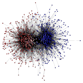
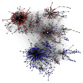
Figure 18: Left: political blog network where node color reflects community membership probability. Right: one example of a forest generated by the Gibbs sampler. The 5 nodes with the larger marker comprise the $95\%$ confidence set for the roots.

6.4 Community discovery with the random $K$ model

For networks with an unknown number of small and possibly overlapping communities, the random $K$ model $\text{PAPER}(\alpha,\beta,\alpha_{0},\theta)$ can be useful for discovering complex community structures. To extract community information from the posterior samples, we again use a greedy matching procedure. To be precise, in the random $K$ setting, our proposed Gibbs sampler outputs a sequence of forests $\tilde{\bm{f}}_{n}^{(1)},\ldots,\tilde{\bm{f}}_{n}^{(J)}$ where $J$ is the number of Monte Carlo samples. We write each forest $\tilde{\bm{f}}_{n}^{(j)}$, for $j\in[J]$, as a collection of trees $\{\tilde{\bm{t}}^{(1,j)},\ldots,\tilde{\bm{t}}^{(K_{j},j)}\}$ where $K_{j}$ is the number of trees in $\tilde{\bm{f}}_{n}^{(j)}$. For $j\in[J]$ and $k\in[K_{j}]$, we write $Q_{k}^{(j)}(\cdot)=\mathbb{P}(\Pi_{1}=\cdot\,|\,\tilde{\bm{T}}=\tilde{\bm{t}}^{(k,j)})$ as the posterior root distribution of the $k$-th tree in the $j$-th Monte Carlo sample. To summarize the output in an interpretable way, we do the following:

1. We initialize $K_{\text{all}}=\max_{j\in[J]}K_{j}$ and $Q_{k}=Q_{k}^{(1)}$ for $k=1,2,\ldots,K_{1}$. For $k=K_{1}+1,\ldots,K_{\text{all}}$, we initialize $Q_{k}(\cdot)=0$.

2. For $j=2,3,\ldots,J$, we match $\{Q_{1},\ldots,Q_{K_{\text{all}}}\}$ with $\{Q_{1}^{(j)},\ldots,Q_{K_{j}}^{(j)}\}$ by computing a one-to-one matching $\sigma\,:\,[K_{j}]\rightarrow[K_{\text{all}}]$ that minimizes

   $$\sum_{k=1}^{K_{j}}\text{TV}(Q_{k}^{(j)},Q_{\sigma(k)}).$$

   For every $k\in[K_{j}]$, if the total variation distance between the $k$-th pair of the matching is too large, that is $\text{TV}(Q_{k}^{(j)},Q_{\sigma(k)})>0.75$, then we create a new set $K_{\text{all}}\leftarrow K_{\text{all}}+1$ and set $Q_{K_{\text{all}}+1}\leftarrow Q_{k}^{(j)}$; otherwise, we perform the update $Q_{\sigma(k)}\leftarrow\frac{j-1}{j}Q_{\sigma(k)}+\frac{1}{j}Q_{k}^{(j)}$.

3. We output $\{Q_{1},\ldots,Q_{K_{\text{all}}}\}$ as the discovered clusters, represented as posterior root probability distributions.

For all of our experiments, we only include trees that contain at least $1\%$ of the total number of nodes. For each discovered cluster $Q_{\ell}$ for $\ell\in[K_{\text{all}}]$, we also compute $\rho_{Q_{\ell}}$ as the number of Monte Carlo iteration $j\in[J]$ where we match $Q_{\ell}$ with $Q_{k}^{(j)}$, i.e. $\sigma(k)=\ell$, and update $Q_{\ell}$. We then compute $\frac{\rho_{Q_{\ell}}}{J}$ as the posterior frequency of cluster $Q_{\ell}$.

In order to check that the random $K$ model is reasonable, we first apply it to the karate club and the political blog networks, which we know contain two underlying clusters, and analyze the resulting posterior distribution over the number of cluster-trees $K$. We provide the results for the karate club network in the left part of Figure 19, in which we see that the posterior mode is at $K=2$. For the political blog network, the Gibbs sampler tends to produce a few large clusters and many tiny clusters of fewer than 10 nodes. Therefore, to compute the posterior over $K$, we count only clusters that have at least 12 nodes (1% of the total number of nodes) and give the results in the right part of Figure 19. The posterior mode in this case is $K=3$, which is reasonably close to the ground truth.

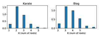
Figure 19: Posterior over $K$ using the random $K$ roots model on the karate club network (left) and the political blog network (right).

We also analyze an air route network (Guimera et al., 2005) of $n=3,618$ airports and $m=14,142$ edges where two airports share an edge if there is a regularly scheduled flight between them. We remove the direction of the edges and treat the network as undirected. The dataset is publicly available at http://seeslab.info/downloads/air-transportation-networks/. Using the random $K$ model, we discover a large central cluster containing major airports around the world and various small clusters that correspond to more remote regions such as airports on Pacific and Polynesian islands, airports in Alaska, and airports in the Canadian Northwest Territories. For sake of brevity, we defer the detailed results to Section S5.2 of the Appendix.

6.5 Analysis of statistician co-authorship network

We now apply PAPER models to perform an extensive analysis of a statistician co-authorship network constructed by Ji and Jin (2016). In this network, each node corresponds to a statistician and two nodes $u$ and $v$ have an edge between them if they have co-authored 1 or more papers in either Journal of Royal Statistical Society: Series B, Journal of the American Statistical Association, Annals of Statistics, or Biometrika from 2002 to 2013. We consider only the largest connected component which has $n=2263$ nodes and $m=4388$ edges. Ji and Jin (2016) in their manuscript (Section 4.3) refers to this network as ”Coauthorship Network (B)”. We emphasize that since the data reflect only coauthorship in 4 journals in the period 2002-2013, the results that we produce cannot be used to compare researchers—we use this network only to illustrate PAPER models in a setting where we can more easily assess whether the output is meaningful or not.

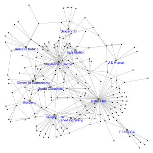
Figure 20: Subgraph of the co-authorship graph comprising the 200 nodes with the highest posterior root probabilities. We label the 12 nodes with the highest root probabilities.

Single root analysis: We first use the single root $\text{PAPER}(\alpha,\beta,\theta)$ model where we estimate $\alpha=0$, $\beta=1$ using the EM algorithm described in Section S3.1. We find that the following 4 nodes have the highest posterior root probabilities: (1) Raymond Carroll with root probability 0.32, (2) Peter Hall with root probability 0.26, (3) Jianqing Fan with root probability 0.086, and (4) James Robins with root probability 0.048. The root probability ranking align closely with betweenness centrality ranking, in which Raymond Carroll, Peter Hall, and Jianqing Fan are also the top 3 most central nodes; see Table 2 of Ji and Jin (2016). Both the root probability ranking and the betweenness ranking differ significantly from degree ranking. We also display the subgraph of the 200 nodes with the highest posterior root probabilities in Figure 20 where we labeled the top 12 nodes with the highest root probabilities.

Community detection with random $K$ roots model: Using our inference algorithm and the greedy matching procedure in 6.4, we compute clusters $\{Q_{1},\ldots,Q_{K_{\text{all}}}\}$ where we find about $K_{\text{all}}\approx 40$ significant clusters. We order the clusters by their posterior frequencies and display the top 9 clusters in Figure 21, along with labels that we curated; we display the nodes in the cluster as word clouds in which the word size is proportional to the posterior root probabilities. We display 18 additional clusters in Section S5.3 of the Appendix. We note that the clusters can overlap since they are constructed from a sequence of posterior samples by matching; see the first paragraph of Section 6.4.

(a) Central super-cluster

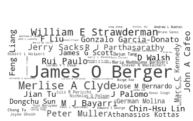
(b) Bayesian

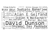
(c) Bayesian

(d) Theory

(e) Multivariate Analysis

(f) Biostat

(g) Computation/UK

(h) Biostat

(i) Graphical Models

Figure 21: Nine of the clusters that most frequently appear in the posterior samples. Word sizes are proportional to the posterior root probability with respect to the cluster.

Ji and Jin (2016) on the same network uses scree plot to conclude that there are $K=3$ clusters, which are shown in Figures 9, 10, and 11 in their paper. They refer to the three clusters as a ”high-dimensional” supercluster, a ”biostatistics” cluster, and a ”Bayes” cluster. We find a giant supercluster, but we also find a large number of smaller clusters which accurately reflect actual research communities in statistics. For example, we find the same ”Bayes” cluster in Ji and Jin (2016) (see Figure 21(b)), but we also discover other Bayesian clusters such as ones shown in Figure 21(c). Similarly, we find the ”biostat” community in Ji and Jin (2016) (see Figure 21(f)) but we find other biostat clusters as well such as the one shown in Figure 21(h) and the one centered on Jason Fine and Michael Korsorok in Figure 27 in the Appendix. In addition, we find many other meaningful communities, such as the experimental design community or the high-dimensional statistics community shown in Figure 22, or the survey and theory community in Figure 27 in the Appendix. We believe that PAPER model gives highly coherent clusters for this network because the network itself is locally tree-like, as shown in two cluster subgraphs that we display in Figure 22.

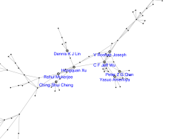
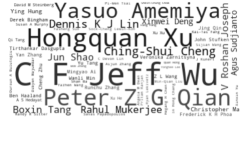
(a) Experimental design community

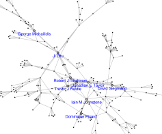
(b) High-dimensional statistics community

Figure 22: Two additional clusters along with the subgraphs that correspond to the clusters. In the subgraph, we label the 8 nodes with the highest posterior root probability with respect to that cluster. We observe that the subgraphs are tree-like.

7 Discussion

In this paper, we present the PAPER model for networks with underlying formation processes and formalize the problem of root inference. We extend the PAPER model to the setting of multiple roots to reflect the growth of multiple communities. There are a number of important open questions from modeling, theoretical, and algorithmic perspectives.

From a modeling perspective, an interesting direction is to suppose that the graph start not as singleton nodes but as a small subgraph. The goal then is to infer the seed-graph instead of the root node (c.f. Devroye and Reddad (2018)). Model extensions such as the PAPER-SBM mixture described in Remark 5 are also interesting; in these models, a subtle question is to what extend we have to estimate the parameters of the noise model well in order to recover the root nodes of the latent forest.

There are many open theoretical questions related to PAPER model and root inference. For instance, in Conjecture 13, we hypothesize that the size of the optimal confidence set for the root node is of a constant order if so long as the noise level is below a certain threshold. If the noise level is above the threshold, then every confidence set has size that diverges with $n$. The lower bound of this conjecture seems especially difficult and may require new techniques. Another interesting theoretical question is the analysis of community recovery using the PAPER model with multiple roots. Intuitively, we expect be able to correctly cluster the early nodes since they tend to have more central positions in the final graph. The late arriving nodes on the other hand would be more peripheral and difficult to cluster.

Algorithmically, we observe that the Gibbs sampler that we derived in Section 4 converges very quickly in practice (see Section S5.4). It would be interesting to study its mixing time, especially how the mixing time depends on the noise level.

Acknowledgement

This work is supported by the U.S. National Science Foundation DMS grant #2113671. The second author is grateful to Justin Khim for insightful discussions in the early stage of the work and to Rong Chen for helpful feedback and comments. The authors would like to thank anonymous referees for insightful comments which helped improve the paper.

List of Figures

Supplementary material to “Root and community inference on latent network growth processes using noisy attachment models”
Harry Crane and Min Xu

S1 Supplement for Section 2

S1.1 Model Likelihood

We first give the likelihood of any time labeled tree under the $\text{APA}(\alpha,\beta)$ model. Define, for any integer $k\geq 1$,

$$\psi_{\alpha,\beta}(k) :=\left\{\begin{array}[]{cc}\prod_{j=1}^{k-1}(\beta j+\alpha)&\text{ if $k\geq 2$, }\\ 1&\text{ if $k=1$. }\end{array}\right.$$

Proposition S1.

Let $\bm{T}_{n}\sim\text{APA}(\alpha,\beta)$. Then, for any time labeled tree $\bm{t}_{n}$, we have that

$$\mathbb{P}(\bm{T}_{n}=\bm{t}_{n})=L_{\alpha,\beta}(\bm{t}_{n}):=\frac{\prod_{v\in[n]}\psi_{\alpha,\beta}(D_{\bm{t}_{n}}(v))}{\prod_{t=3}^{n}(2(t-2)\beta+(t-1)\alpha)}.$$ (S1.1)

The fact that the likelihood depends on the tree $\bm{t}_{n}$ only through its degree distribution $D_{\bm{t}_{n}}(\cdot)$ remains true in the multiple roots setting except that the likelihood also depends on the root nodes. One complication with the multiple roots setting is that we give each root node an imaginary self-loop. To deal with this, we first define $\psi^{r}_{\alpha,\beta}(k):=\prod_{j=2}^{k+1}(\beta j+\alpha)$.

Proposition S2.

Let $\bm{F}_{n}\sim\text{APA}(\alpha,\beta,K)$. Then, for any time labeled forest $\bm{f}_{n}$, we have that

$$\mathbb{P}(\bm{F}_{n}=\bm{f}_{n})=L_{\alpha,\beta,K}(\bm{f}_{n}):=\frac{\prod_{v\in\pi_{1:K}}\psi_{\alpha,\beta}^{r}(D_{\bm{f}_{n}}(v))\prod_{v\notin\pi_{1:K}}\psi_{\alpha,\beta}(D_{\bm{f}_{n}}(v))}{\prod_{t=K+1}^{n}(2(t-1)\beta+(t-1)\alpha)}.$$ (S1.2)

In the random $K$ setting, the likelihood is very similar except that the set of root nodes is not necessarily $\pi_{1:K}$.

Proposition S3.

Let $\bm{F}_{n}\sim\text{APA}(\alpha,\beta,\alpha_{0})$. Then, for any time labeled forest $\bm{f}_{n}$ with $K$ component trees, we have that

$$\mathbb{P}(\bm{F}_{n}=\bm{f}_{n})=L_{\alpha,\beta,S}(\bm{f}_{n}):=\frac{\prod_{v\in S}\psi_{\alpha,\beta}^{r}(D_{\bm{f}_{n}}(v))\prod_{v\notin S}\psi_{\alpha,\beta}(D_{\bm{f}_{n}}(v))}{\prod_{t=K+1}^{n}(2(t-1)\beta+(t-1)\alpha)}.$$ (S1.3)

where $S$ is the set of root nodes of $\bm{f}_{n}$, that is, a node is in $S$ if and only if it has the earliest arrival time in its component tree.

Under the PAPER model, the complete data likelihood is also simple owing to the fact that any non-forest edge of the random graph $\bm{G}_{n}$ is Erdős–Rényi and any forest with $K$ component trees has exactly $n-K$ edges. Therefore, for a time labeled graph $\bm{g}_{n}$ with $m$ edges and a time labeled sub-forest $\bm{f}_{n}$, we have that, under the PAPER model and conditional on $\bm{G}_{n}$ having $m$ edges,

$$\mathbb{P}(\bm{G}_{n}=\bm{g}_{n},\bm{F}_{n}=\bm{f}_{n})=\binom{n(n-1)/2-(n-K)}{m-(n-K)}^{-1}\mathbb{P}(\bm{F}_{n}=\bm{f}_{n}).$$

We do not observe the forest of course. This is one of the main hurdles that we address in Section 4.

S1.2 Poisson attachment approximation

Proposition S4.

Let $t\in\mathbb{N}$, and let $q_{1},\ldots,q_{t}\in[0,1]$ satisfy $\sum_{j=1}^{t}q_{j}\leq 1$, and let $\theta>0$ such that $\theta q_{j}\leq 1$ for all $i\in[t]$. Let $X$ and $Y$ denote two random subsets of $[t]$, where $X$ is generated by adding each $j\in[t]$ independently with probability $\theta q_{j}$, and where $Y$ is generated by first drawing $M\sim\text{Poisson}(\theta)$ and then repeating $M$ times the procedure where we randomly choose $j\in[t]$ with probability $q_{j}$ and with replacement and add $j$ to $Y$. Let $P^{(X)}$ and $P^{(Y)}$ denote the distribution of $X$ and $Y$ respectively. Then, we have that

$$d_{\text{TV}}(P^{(X)},P^{(Y)})\leq\theta^{2}\max_{j\in[t]}q_{j}.$$

Proof.

For $j=1,\ldots,n$, define $X_{j}=\mathbbm{1}\{j\in X\}$ and $Y_{j}$ as the number of copies of element $j$ in $Y$. Direct calculation then shows that $X_{1},\ldots,X_{t}$ are independent where $X_{j}\sim\text{Ber}(\theta q_{j})$ and that $Y_{1},\ldots,Y_{t}$ are independent where $Y_{j}\sim\text{Poisson}(\theta q_{j})$.

Therefore, by a coupling argument (see e.g. Example 2 in Chapter 10.1 of Pollard (2002)) and the fact that $\sum_{j=1}^{t}q_{j}\leq 1$, we have

$$d_{\text{TV}}(P^{(X)},P^{(Y)}) \leq\mathbb{P}(X\neq Y)=\sum_{j=1}^{t}\mathbb{P}(X_{j}\neq Y_{j})$$

$$\leq\sum_{j=1}^{t}\theta^{2}q_{j}^{2}\leq\theta^{2}\max_{j}q_{j},$$

as desired. ∎

If we apply Proposition S4 to the independent Bernoulli noise model described in Section 2.3, where $X$ and $Y$ denote the random set of edges added under the Bernoulli noise model and the Poisson noise model respectively and where $q_{j}=\frac{\tilde{\beta}D_{\bm{T}_{t-1}}(j)+\tilde{\alpha}}{2(t-2)\tilde{\beta}+(t-1)\tilde{\alpha}}$, then we may use the fact that $\max_{j\in[t]}q_{j}=O_{p}(\frac{1}{\sqrt{t}})$ (see e.g. Section 8.7 in Van Der Hofstad (2016)) to see that the two noise models are approximately equivalent for large $t$.

S2 Supplement for Section 3

Recall that for an alphabetically labeled tree $\tilde{\bm{t}}_{n}$, we define the $\text{hist}(\tilde{\bm{t}}_{n})$ as the set of all label ordering $\pi\in\text{Bi}([n],\mathcal{U}_{n})$ such that $\pi^{-1}\tilde{\bm{t}}_{n}$ is a time labeled tree that has a positive probability over the APA model (Definition 1). For a node $u$, we also define $\text{hist}(u,\tilde{\bm{t}}_{n})$ as all $\pi\in\text{hist}(\tilde{\bm{t}}_{n})$ such that $\pi_{1}=u$ and $h(u,\tilde{\bm{t}}_{n})=|\text{hist}(u,\tilde{\bm{t}}_{n})|$. Shah and Zaman (2011) derives an $O(n)$ runtime algorithm that computes the whole collection $\{h(u,\tilde{\bm{t}}_{n})\}_{u\in\mathcal{U}_{n}}$, which is shown as Algorithm 4.

Algorithm 4 Computing $\{h(u,\tilde{\mathbf{t}}_{n})\}_{u\in\mathcal{U}_{n}}$ (Shah and Zaman; 2011)

Input: a labeled tree $\tilde{\mathbf{t}}_{n}$.
Output: $h(u,\tilde{\mathbf{t}}_{n})$ for all nodes $u\in\mathcal{U}_{n}$.

Arbitrarily select root $u_{0}\in\mathcal{U}_{n}$.

for $u\in\mathcal{U}_{n}$ do

     Compute and store $n^{(u_{0})}_{u}:=|\tilde{\mathbf{t}}^{(u_{0})}_{u}|$.

end for

Compute $h(u_{0},\tilde{\mathbf{t}}_{n})=n!\prod_{u\in\mathcal{U}_{n}}\frac{1}{|\tilde{\bm{t}}^{(u_{0})}_{u}|}$.

Set $\mathcal{S}=\{\text{Children}(u_{0})\}$.

while $\mathcal{S}$ is not empty do

     Remove an arbitrary node $u\in\mathcal{S}$.

     Compute $h(u,\tilde{\mathbf{t}}_{n})=h(\text{pa}(u),\tilde{\mathbf{t}}_{n})\frac{n_{u}^{(u_{0})}}{n-n_{u}^{(u_{0})}}$

     Add $\text{Children}(u)$ to $\mathcal{S}$

end while

S2.1 Equivalence to maximum likelihood

Before deriving the likelihood formally, it is useful to have the following standard definitions. For two labeled graphs $\bm{g},\bm{g}^{\prime}$, we say that $\bm{g}\sim\bm{g}^{\prime}$ if there exists $\rho\in\text{Bi}(V(\bm{g}),V(\bm{g}^{\prime}))$ such that $\rho\bm{g}=\bm{g}^{\prime}$. In this case, we say that $\bm{g}$ and $\bm{g}^{\prime}$ are isomorphic, or that they have the same shape, or that they are equivalent as unlabeled graphs. The $\sim$ relationship defines equivalence classes on the set of all labeled graphs, which we refer to as the unlabeled shape or just shape for short. We write

$$I(\bm{g},\bm{g^{\prime}}):=\{\rho\in\text{Bi}(V(\bm{g}),V(\bm{g}^{\prime}))\,:\,\rho\bm{g}=\bm{g}^{\prime}\}.$$

Note that $I(\bm{g},\bm{g})$ is the set of automorphisms of the graph $\bm{g}$. To represent an unlabeled shape, we write $\text{sh}(\bm{g})$ where $\bm{g}$ an arbitrary representative element in the equivalence class.

Similarly, given a node $u\in V(\bm{g})$ and $u^{\prime}\in V(\bm{g}^{\prime})$, we say that $(\bm{g},u)\sim_{0}(\bm{g}^{\prime},u^{\prime})$ if there exists $\rho\in\text{Bi}(V(\bm{g}),V(\bm{g}^{\prime}))$ such that $\rho\bm{g}=\bm{g}^{\prime}$ and $\rho(u)=u^{\prime}$. In this case, we say that $(\bm{g},u)$ and $(\bm{g}^{\prime},u^{\prime})$ have the same rooted shape. The $\sim_{0}$ relationship defines an equivalence class on the pairs $(\bm{g},u)$. We write

$$I(\bm{g},u,\bm{g^{\prime}},u^{\prime}):=\{\rho\in\text{Bi}(V(\bm{g}),V(\bm{g}^{\prime}))\,:\,\rho\bm{g}=\bm{g}^{\prime},\rho(u)=u^{\prime}\}.$$

We have the following facts:

1. $I(\bm{g},\bm{g}^{\prime})$ is non-empty if and only if $\bm{g},\bm{g}^{\prime}$ have the same shape. Moreover, the cardinality of $I(\bm{g},\bm{g}^{\prime})$ depends only on that shape. For instance, $|I(\bm{g},\bm{g}^{\prime})|=|I(\bm{g},\bm{g})|$ if the former is non-zero. In discrete mathematics, this cardinality is referred to as the size of the automorphism group of $\bm{g}$.

2. $I(\bm{g},u,\bm{g}^{\prime},u^{\prime})$ is non-empty if and only if $(\bm{g},u),(\bm{g}^{\prime},u^{\prime})$ have the same shape. Moreover, the cardinality of $I(\bm{g},u,\bm{g}^{\prime},u^{\prime})$ depends only on that shape.

Now, for a labeled graph $\bm{g}$ and a node $u\in V(\bm{g})$, we define

$$\text{Eq}(u,\bm{g})=\{u^{\prime}\in\bm{g}\,:\,(\bm{g},u)\sim_{0}(\bm{g},u^{\prime})\}.$$

Nodes in $\text{Eq}(u,\bm{g})$ are indistinguishable from node $u$ once the node labels are removed.

On observing an unlabeled graph $\text{sh}(\tilde{\bm{g}}_{n})$, the likelihood of a node $u$ being the root node is therefore

$$\mathcal{L}(u,\tilde{\bm{g}}_{n}):=\frac{1}{|\text{Eq}(u,\tilde{\bm{g}}_{n})|}\sum_{\bm{g}_{n}\text{ time labeled}}\mathbb{P}(\bm{G}_{n}=\bm{g}_{n})\mathbbm{1}\{(\bm{g}_{n},1)\sim_{0}(\tilde{\bm{g}}_{n},u)\},$$

where $\bm{G}_{n}$ has the $\text{PAPER}(\alpha,\beta,\theta)$ distribution. It is straightforward to check that $\mathcal{L}(u,\tilde{\bm{g}}_{n})$ depends only on the unlabeled shape of $(\tilde{\bm{g}}_{n},u)$. We give a concrete example of the likelihood in Figure 23.

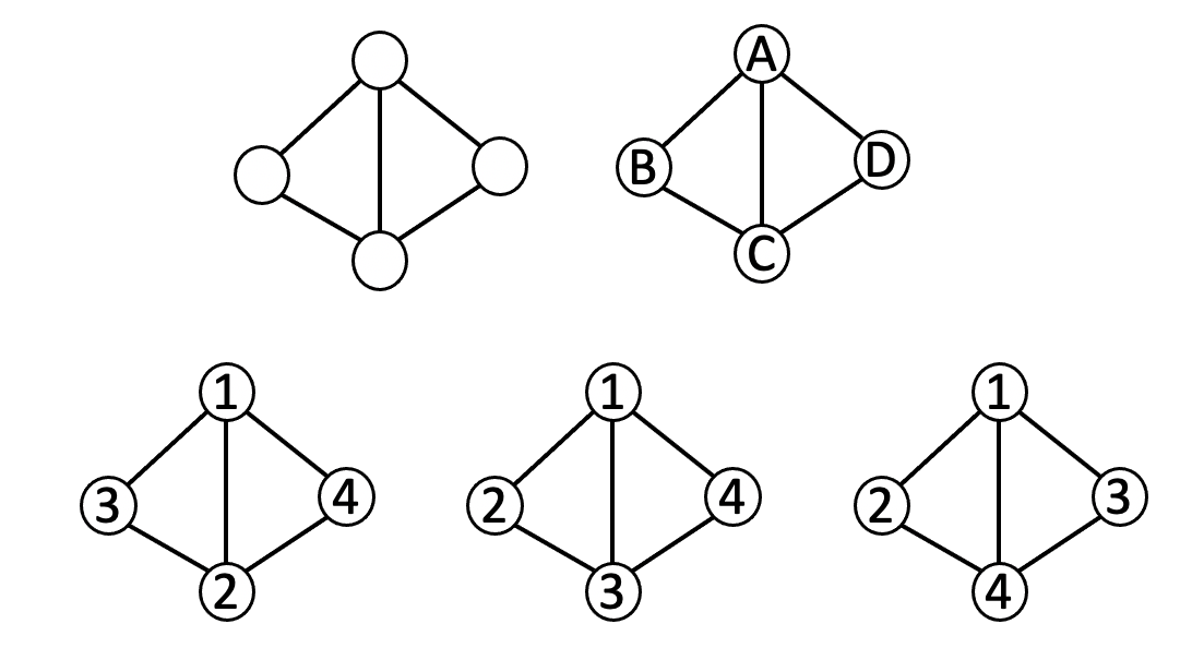
Figure 23: Viewing the top right graph as $\tilde{\bm{g}}$ and the bottom graphs as $\bm{g}^{1},\bm{g}^{2},\bm{g}^{3}$, we have $\text{Eq}(A,\tilde{\bm{g}})=\{A,C\}$ and $\mathcal{L}(A,\tilde{\bm{g}}_{n})=\frac{1}{2}\bigl{\{}\mathbb{P}(\bm{G}_{n}=\bm{g}^{1})+\mathbb{P}(\bm{G}_{n}=\bm{g}^{2})+\mathbb{P}(\bm{G}_{n}=\bm{g}^{3})\bigr{\}}$.

Theorem S5.

For any alphabetically labeled graph $\tilde{\bm{g}}_{n}$, we have

$$\mathbb{P}(\Pi_{1}=u\,|\,\tilde{\bm{G}}_{n}=\tilde{\bm{g}}_{n})=\frac{\mathcal{L}(u,\tilde{\bm{g}}_{n})}{\sum_{v\in\mathcal{U}_{n}}\mathcal{L}(v,\tilde{\bm{g}}_{n})}.$$

Proof.

We have that

$$\mathbb{P}(\Pi_{1}=u\,|\,\tilde{\bm{G}}_{n}=\tilde{\bm{g}}_{n}) \propto\sum_{\pi\in\text{Bi}([n],\mathcal{U}_{n}),\,\pi_{1}=u}\mathbb{P}(\tilde{\bm{G}}_{n}=\tilde{\bm{g}}_{n}\,|\,\Pi=\pi)\frac{1}{n!}$$

$$\propto\sum_{\pi\in\text{Bi}([n],\mathcal{U}_{n}),\,\pi_{1}=u}\mathbb{P}(\bm{G}_{n}=\pi^{-1}\tilde{\bm{g}}_{n})$$

$$=\sum_{\bm{g}_{n}\text{ time labeled}}\sum_{\stackrel{{\scriptstyle\pi\in\text{Bi}([n],\mathcal{U}_{n}),}}{{\pi_{1}=u,\pi\bm{g}_{n}=\tilde{\bm{g}}_{n}}}}\mathbb{P}(\bm{G}_{n}=\bm{g}_{n})$$

$$=\sum_{\bm{g}_{n}\text{ time labeled}}|I(\bm{g}_{n},1,\tilde{\bm{g}}_{n},u)|\mathbb{P}(\bm{G}_{n}=\bm{g}_{n})$$

$$=\frac{|I(\tilde{\bm{g}}_{n},\tilde{\bm{g}}_{n})|}{|\text{Eq}(u,\tilde{\bm{g}}_{n})|}\sum_{\bm{g}_{n}\text{ time labeled}}\mathbb{P}(\bm{G}_{n}=\bm{g}_{n})\mathbbm{1}\{(\bm{g}_{n},1)\sim_{0}(\tilde{\bm{g}}_{n},u)\},$$

where the second equality follows by the definition of $I(\bm{g},1,\tilde{\bm{g}}_{n},u)$ and the final equality follows by Lemma S6. The desired conclusion immediately follows.

∎

Lemma S6.

For any labeled graphs $\bm{g},\bm{g}^{\prime}$ and nodes $u\in V(\bm{g})$, $u^{\prime}\in V(\bm{g}^{\prime})$, if $(\bm{g},u)\sim_{0}(\bm{g}^{\prime},u^{\prime})$, then

$$|I(\bm{g},\bm{g^{\prime}})|=|I(\bm{g},u,\bm{g}^{\prime},u^{\prime})||\text{Eq}(u,\bm{g})|.$$

Proof.

Suppose $|I(\bm{g},u,\bm{g}^{\prime},u^{\prime})|>0$. We note for any node $v\in V(\bm{g})$, we have that $|I(\bm{g},v,\bm{g}^{\prime},u^{\prime})|$ is either zero or equal to $|I(\bm{g},u,\bm{g}^{\prime},u^{\prime})|$. Moreover, it is non-zero if and only if $v\in\text{Eq}(u,\bm{g})$.

Therefore, using the fact that $I(\bm{g},\bm{g}^{\prime})=\cup_{v\in V(\bm{g})}I(\bm{g},v,\bm{g}^{\prime},u^{\prime})$, we have

$$|I(\bm{g},\bm{g^{\prime}})|=\sum_{v\in V(\bm{g})}|I(\bm{g},v,\bm{g}^{\prime},u^{\prime})|=|\text{Eq}(u,\bm{g}_{n})||I(\bm{g},u,\bm{g}^{\prime},u^{\prime})|,$$

as desired. ∎

S3 Supplement for Section 4

S3.1 Parameter estimation for the PAPER model via EM

The PAPER models are parametrized by $\alpha,\beta$ which control the attachment mechanism, by $\theta$ which is the noise level, and by either $K$ or $\alpha_{0}$ in the multiple roots setting. We discuss some ways to select the number of trees $K$ in the fixed $K$ root setting and ways to estimate $\alpha_{0}$ in the random $K$ roots setting in Section S3.4 of the appendix.

In this section therefore, we consider only the estimation of the parameters $\alpha$ and $\beta$. We assume that $\beta>0$, in which case, without loss of generality, we may assume $\beta=1$ so that we only need to estimate $\alpha$. We note that assuming $\beta>0$ does not exclude uniform attachment if we allow $\alpha=\infty$. We first consider the single root setting. For any tree $\tilde{\bm{t}}_{n}$, by Proposition S1 that

$$\mathbb{P}_{\alpha}(\tilde{\bm{T}}_{n}=\tilde{\bm{t}}_{n}) =\sum_{\pi\in\text{hist}(\tilde{\bm{t}}_{n})}\mathbb{P}_{\alpha}(\bm{T}_{n}=\pi^{-1}\tilde{\bm{t}}\,|\,\Pi=\pi)\mathbb{P}(\Pi=\pi)$$

$$=h(\tilde{\bm{t}}_{n})\frac{\prod_{v\in\mathcal{U}_{n}}\prod_{j=1}^{D_{\tilde{\bm{t}}_{n}}(v)-1}(j+\alpha)}{\prod_{k=3}^{n}(2(k-2)+(k-1)\alpha)}\frac{1}{n!}.$$ (S3.4)

Therefore, keeping only terms that depend on $\alpha$, we have that the log-likelihood is

$$\ell(\alpha;\tilde{\bm{T}}_{n}) =\sum_{v\in\mathcal{U}_{n}}\sum_{j=1}^{\infty}\log(j+\alpha)\mathbbm{1}\{j<D_{\tilde{\bm{T}}_{n}}(v)\}-\sum_{k=3}^{n}\log\bigl{(}2(k-2)+(k-1)\alpha\bigr{)}$$

$$=\sum_{j=1}^{\infty}\log(j+\alpha)W_{\tilde{\bm{T}}_{n}}(j)-\sum_{k=3}^{n}\log\bigl{(}2(k-2)+(k-1)\alpha\bigr{)},$$

where we define $W_{\tilde{\bm{T}}_{n}}(j):=|\{v\in\mathcal{U}_{n}\,:\,D_{\tilde{\bm{T}}_{n}}(v)>j\}|$. We note that, in this case, the log-likelihood of $\alpha$ depends on the tree $\tilde{\bm{T}}_{n}$ only through its degree sequence.

In the PAPER model where $\tilde{\bm{G}}_{n}=\tilde{\bm{T}}_{n}+\tilde{\bm{R}}_{n}$, for every node $v\in\mathcal{U}_{n}$, we have that $D_{\tilde{\bm{G}}_{n}}(v)=D_{\tilde{\bm{T}}_{n}}(v)+D_{\tilde{\bm{R}}_{n}}(v)$ where the tree degree $D_{\tilde{\bm{T}}_{n}}(v)$ is now latent. We propose an approximate EM algorithm in this setting.

The complete data log-likelihood in this case is

$$\ell(\alpha;D_{\tilde{\bm{G}}_{n}},D_{\tilde{\bm{T}}_{n}})=\sum_{j=1}^{\infty}\log(j+\alpha)\sum_{v}\mathbbm{1}\{j<D_{\tilde{\bm{T}}_{n}}(v)\}-\sum_{k=s}^{n}\log\bigl{(}2(k-2)+(k-1)\alpha\bigr{)}.$$

For a given value $\alpha^{\prime}$, the EM update is then to maximize

$$M(\alpha|\alpha^{\prime}) :=\mathbb{E}_{\alpha^{\prime}}\biggl{[}\sum_{j=1}^{\infty}\log(j+\alpha)\sum_{v}\mathbbm{1}\{j<D_{\tilde{\bm{T}}_{n}}(v)\}\,\bigg{|}\,\tilde{\bm{G}}_{n}\biggr{]}-\sum_{k=s}^{n}\log\bigl{(}2(k-2)+(k-1)\alpha\bigr{)}$$

$$=\sum_{j=1}^{\infty}\log(j+\alpha)\sum_{v}\mathbb{P}_{\alpha^{\prime}}\biggl{\{}j<D_{\tilde{\bm{T}}_{n}}(v)\,\bigg{|}\,\tilde{\bm{G}}_{n}\biggr{\}}-\sum_{k=s}^{n}\log\bigl{(}2(k-2)+(k-1)\alpha\bigr{)}.$$ (S3.5)

The conditional probability term $\mathbb{P}_{\alpha^{\prime}}(j<D_{\tilde{\bm{T}}_{n}}(v)\,|\,\tilde{\bm{G}}_{n})$ can be computed by Gibbs sampling, but we can significantly reduce the computation time by approximating $\mathbb{P}_{\alpha^{\prime}}(j<D_{\tilde{\bm{T}}_{n}}(v)\,|\,\tilde{\bm{G}}_{n})$ with $\mathbb{P}_{\alpha^{\prime}}(j<D_{\tilde{\bm{T}}_{n}}(v)\,|\,D_{\tilde{\bm{G}}_{n}}(v))$, which ignores the mild dependence between the degrees of all the nodes. To further improve the quality of the approximation, we observe that

$$\sum_{j=1}^{\infty}\sum_{v}\mathbb{P}_{\alpha^{\prime}}\bigl{(}j<D_{\tilde{\bm{T}}_{n}}(v)\,\big{|}\,\tilde{\bm{G}}_{n}\bigr{)}=\sum_{v}(D_{\tilde{\bm{T}}_{n}}(v)-1)=n-2$$

while the sums of the approximate conditional probabilities $\sum_{j=1}^{\infty}\sum_{v}\mathbb{P}_{\alpha^{\prime}}(j<D_{\tilde{\bm{T}}_{n}}(v)\,|\,D_{\tilde{\bm{G}}_{n}}(v))$ may be different. Thus, we normalize $\mathbb{P}_{\alpha^{\prime}}(j<D_{\tilde{\bm{T}}_{n}}(v)\,|\,D_{\tilde{\bm{G}}_{n}}(v))$ by defining $\tilde{W}_{\tilde{\bm{G}}_{n}}(j)=(n-2)\frac{\mathbb{P}_{\alpha^{\prime}}(j<D_{\tilde{\bm{T}}_{n}}(v)\,|\,D_{\tilde{\bm{G}}_{n}}(v))}{\sum_{j=1}^{\infty}\mathbb{P}_{\alpha^{\prime}}(j<D_{\tilde{\bm{T}}_{n}}(v)\,|\,D_{\tilde{\bm{G}}_{n}}(v))}$ so that $\sum_{j=1}^{\infty}\tilde{W}_{\tilde{\bm{G}}_{n}}(j)=n-2$ and, instead of maximizing (S3.5), we update

$$\tilde{M}(\alpha|\alpha^{\prime}):=\sum_{j=1}^{\infty}\log(j+\alpha)\tilde{W}_{\tilde{\bm{G}}_{n}}(j)-\sum_{k=s}^{n}\log\bigl{(}2(k-2)+(k-1)\alpha\bigr{)}.$$ (S3.6)

In practice, we find that the normalization significant improves the quality of the approximation.

To compute $\tilde{W}_{\tilde{\bm{G}}_{n}}$, we have by Bayes rule that for any $k\in[n]$ and $s\leq k$,

$$\mathbb{P}_{\alpha^{\prime}}(D_{\tilde{\bm{T}}_{n}}(v)=s\,|\,D_{\tilde{\bm{G}}_{n}}(v)=k) =\frac{\mathbb{P}_{\alpha^{\prime}}(D_{\tilde{\bm{T}}_{n}}(v)=s,D_{\tilde{\bm{R}}_{n}}(v)=k-s)}{\sum_{t=1}^{k}\mathbb{P}_{\alpha^{\prime}}(D_{\tilde{\bm{T}}_{n}}(v)=t,D_{\tilde{\bm{R}}_{n}}(v)=k-t)}$$ (S3.7)

$$=\frac{P_{\text{Bin}(n-s,\theta)}(k-s)\mathbb{P}_{\alpha^{\prime}}(D_{\tilde{\bm{T}}_{n}}(v)=s)}{\sum_{t=1}^{k}P_{\text{Bin}(n-t,\theta)}(k-t)\mathbb{P}_{\alpha^{\prime}}(D_{\tilde{\bm{T}}_{n}}(v)=t)},$$ (S3.8)

where $P_{\text{Bin}(n-s,\theta)}(\cdot)$ denotes the probability of a binomial distribution with $n-s$ trials and success probability $\theta$. The exact distribution of the degree $D_{\tilde{\bm{T}}_{n}}(v)$ of a node $v$ under the $\text{APA}_{\alpha^{\prime},1}$ is intractable but we can approximate it by its limiting distribution

$$P_{\alpha^{\prime}}(s):=(2+\alpha^{\prime})\frac{\Gamma(s+\alpha^{\prime})\Gamma(3+2\alpha^{\prime})}{\Gamma(s+3+2\alpha^{\prime})\Gamma(1+\alpha^{\prime})}=\frac{2+\alpha^{\prime}}{3+2\alpha^{\prime}}\prod_{j=1}^{s-1}\frac{j+\alpha^{\prime}}{j+3+2\alpha^{\prime}}.$$

By Van Der Hofstad (Theorem 8.2 2016), we have that, for any node $v$,

$$\sup_{s\in\mathbb{N}}\bigl{|}\mathbb{P}_{\alpha^{\prime}}\bigl{(}D_{\tilde{\bm{T}}_{n}}(v)=s\bigr{)}-P_{\alpha^{\prime}}(s)\bigr{|}\leq C_{\alpha^{\prime}}\sqrt{\frac{\log n}{n}}$$

with probability that tends to 1 as $n\rightarrow\infty$. Therefore, we may replace $\mathbb{P}_{\alpha^{\prime}}\bigl{(}D_{\tilde{\bm{T}}_{n}}(v)=s\bigr{)}$ with $P_{\alpha^{\prime}}(s)$ in (S3.8) to obtain a tractable approximation which is accurate in the limit.

To summarize, our estimation procedure generates a sequence $\alpha^{j}$ where $\alpha^{j}$ maximizes $\tilde{M}(\cdot\,|\,\alpha^{j-1})$ and where $\tilde{M}$ is computed using (S3.8). Although we approximate $M(\cdot\,|\,\cdot)$ by $\tilde{M}(\cdot\,|\,\cdot)$ and approximate the distribution of the random degree $D_{\tilde{\bm{T}}_{n}}(v)$ by its asymptotic limit, we find empirically that the resulting procedure always converges and performs well. We test the estimation procedure on simulated PAPER graphs of $n=3,000$ nodes and $m=15,000$ edges and report the estimation performance in Table 6. We find that the estimator is biased upwards when $\alpha$ is large, which is possibly because the likelihood (S3.4) is much less sensitive to a change in $\alpha$ when $\alpha$ is large than when $\alpha$ is small. In our simulation studies (Section 6.1), we show that the confidence sets constructed with the estimated parameters still attain their nominal coverage so that estimation error does not significantly impact the inference quality.

True $\alpha$	0	1	3	6	$\infty$ (UA)
Estimated $\alpha$	0.03 (0.04)	1.04 (0.2)	3.3 (1.34)	10.7 (13.57)	85.4 (20.9)

Table 6: Mean and standard deviation of the estimated $\alpha$ computed on 200 independent trials on graphs with $n=3,000$ nodes and $m=15,000$ edges.

We use the same estimator in the fixed $K>1$ setting and the variable $K$ setting. In these cases, the log-likelihood is slightly different because the root nodes have imaginary self-loop edges. However, if the number of root nodes is small, the log-likelihood is virtually identical.

S3.2 Derivation of root sampling probability (22) for the fixed $K$ and random $K$ setting

Let $\tilde{\bm{f}}_{n}$ be an alphabetically labeled forest with component trees $\tilde{\bm{t}}^{1},\ldots,\tilde{\bm{t}}^{K}$. For a specific tree $\tilde{\bm{t}}^{k}$ and a node $u\in V(\tilde{\bm{t}}^{k})\subset\mathcal{U}_{n}$, we compute the probability, under the $\text{PAPER}(\alpha,\beta,K,\theta)$ model and label randomization, that $u^{k}$ is the first node of $\tilde{\bm{t}}^{k}$ given $\tilde{\bm{F}}_{n}=\tilde{\bm{f}}_{n}$.

To formally derive this, denote the $K$ random component trees of the random forest $\tilde{\bm{F}}_{n}$ by $\tilde{\bm{T}}^{1},\ldots,\tilde{\bm{T}}^{K}$, and define $\Pi^{k}$ as the random latent relative ordering of the nodes in the $k$-th random component tree $\tilde{\bm{T}}^{k}$. In other words, $\Pi^{k}$ takes value in $\text{Bi}([n^{k}],V(\tilde{\bm{T}}^{k}))$ (where $n^{k}=|V(\tilde{\bm{T}}^{k})|$) and $\Pi^{k}_{t}=v$ implies that $v$ is the $t$-th node, among the nodes of $\tilde{\bm{T}}^{k}$, to arrive in $\tilde{\bm{T}}^{k}$.

Then, we have that, for any $u\in V(\tilde{\bm{t}}^{k})$,

$$\mathbb{P}(\Pi^{k}_{1}=u\,|\,\tilde{\bm{T}}^{k}=\tilde{\bm{t}}^{k}) =\sum_{\pi^{k}\in\text{hist}(u,\tilde{\bm{t}}^{k})}\mathbb{P}(\Pi^{k}=\pi^{k}\,|\,\tilde{\bm{T}}^{k}=\tilde{\bm{t}}^{k})$$

$$\propto\sum_{\pi^{k}\in\text{hist}(u,\tilde{\bm{t}}^{k})}\mathbb{P}(\tilde{\bm{T}}^{k}=\tilde{\bm{t}}^{k}\,|\,\Pi^{k}=\pi^{k})$$

$$\propto h(u,\tilde{\bm{t}}^{k})\prod_{j=2}^{D_{\tilde{\bm{t}}^{k}}(u)+1}(\beta j+\alpha)\prod_{v\neq u,v\in V(\tilde{\bm{t}}^{k})}\prod_{j=1}^{D_{\tilde{\bm{t}}^{k}}(v)-1}(\beta j+\alpha)$$

$$=h(u,\tilde{\bm{t}}^{k})(\beta D_{\tilde{\bm{t}}^{k}}(u)+\beta+\alpha)(\beta D_{\tilde{\bm{t}}^{k}}(u)+\alpha)\prod_{v\in V(\tilde{\bm{t}}^{k})}\prod_{j=1}^{D_{\tilde{\bm{t}}^{k}}(v)-1}(\beta j+\alpha)$$

$$\propto h(u,\tilde{\bm{t}}^{k})(\beta D_{\tilde{\bm{t}}^{k}}(u)+\beta+\alpha)(\beta D_{\tilde{\bm{t}}^{k}}(u)+\alpha),$$

where the third proportionality (equality up to multiplicative factor that is constant with respect to $u$) follows from Proposition S2. Formula (22) thus follows.

S3.3 Collapsed Gibbs sampler

We give an alternative Gibbs sampler in which we sample only a set of root nodes instead of sampling an entire history $\pi$. More precisely, we alternate between the following two stages:

1. We fix the forest $\tilde{\bm{f}}$ and sample a set of root nodes $\tilde{s}$ with probability

   $$\mathbb{P}(\tilde{S}=\tilde{s}\,|\,\tilde{\bm{F}}_{n}=\tilde{\bm{f}}_{n},\tilde{\bm{G}}_{n}=\tilde{\bm{g}})\propto\mathbb{P}(\tilde{S}=\tilde{s}\,|\,\tilde{\bm{F}}_{n}=\tilde{\bm{f}}_{n}),$$ (S3.9)

   where $\tilde{s}$ comprise of a single node from each of the component trees of $\tilde{\bm{f}}_{n}$.

2. We fix the root set $\tilde{s}$ and generate a new forest $\tilde{\bm{f}}_{n}$ by iteratively sampling a new parent for each of the nodes.

To sample the root set for the first stage of the Gibbs sampler, we write $\tilde{\bm{t}}^{1},\ldots,\tilde{\bm{t}}^{K}$ as the $K$ disjoint trees of the fixed forest $\tilde{\bm{f}}_{n}$. Then, to generate the root set $\tilde{s}$, we generate, for each tree $\tilde{\bm{t}}^{k}$, the root node $u^{k}$ with probability (22).

For the second stage of the Gibbs sampler, we place the nodes in some arbitrary order and for each node $u$, we generate a parent $\tilde{u}$, which could be equal to the old parent, according to the distribution

$$\mathbb{P}\bigl{\{}pa(u)=\tilde{u}\,|\,\{pa(v)\}_{v\neq u},\tilde{S}=\tilde{s},\tilde{\bm{G}}_{n}=\tilde{\bm{g}}_{n}\bigr{\}}.$$ (S3.10)

The action of generating a new parent is equivalent to replacing the edge between $u$ and its old parent with a new one between $u$ and $\tilde{u}$. Because we do not condition on the ordering $\Pi$, the new parent $\tilde{u}$ can be any node in the network connected to $u$ that is not a descendant of $u$–that is, we only require that $\tilde{u}$ is not in the subtree $\tilde{\bm{t}}^{(\tilde{s})}_{u}$ of node $u$, where we view $\tilde{s}$ as the roots for the whole forest.

Another way to think of the second stage is that we take the subtree $\tilde{\bm{t}}^{(\tilde{s})}_{u}$ and graft it onto another part of the forest. In the multiple roots setting, a subtree may be transferred from one component tree to another. In the random $K$ setting, two disjoint subtrees may be merged into a single tree or, a subtree may be split and forms a new component. See Figure 24 for a visual illustration.

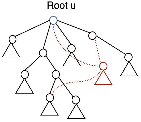
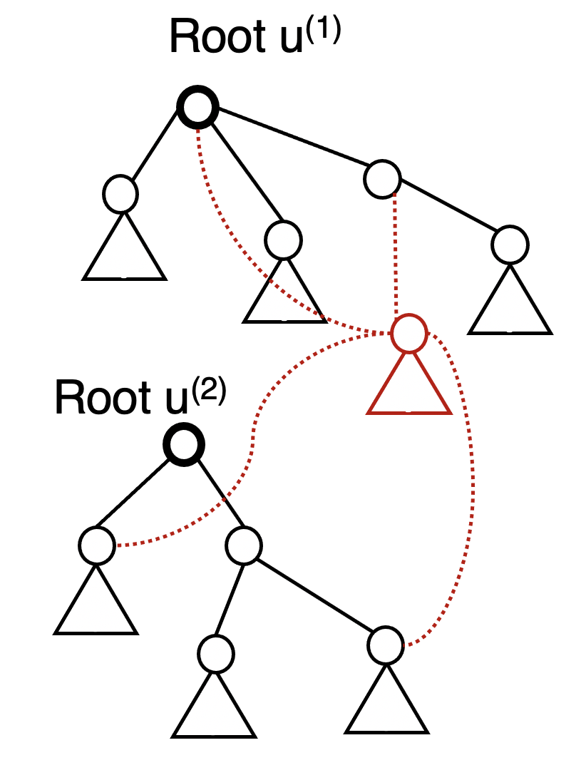
Figure 24: Selecting a new parent for a node. Left: the single root setting. Right: the multiple roots setting.

In contrast with (28), we do not condition on $\Pi$ and must therefore sum over all histories when computing (S3.10):

$$\mathbb{P}(\tilde{\bm{F}}_{n}=\tilde{\bm{f}}_{n}\,|\,\tilde{\bm{G}}_{n}=\tilde{\bm{g}}_{n},\tilde{S}=\tilde{s})$$

$$\qquad\propto\mathbb{P}(\tilde{\bm{G}}_{n}=\tilde{\bm{g}}_{n}\,|\,\tilde{\bm{F}}_{n}=\tilde{\bm{f}}_{n})\mathbb{P}(\tilde{\bm{F}}_{n}=\tilde{\bm{f}}_{n},\tilde{S}=\tilde{s})$$

$$\qquad=\binom{n(n-1)/2-n+K}{m-n+k}^{-1}\sum_{\pi\in\text{hist}(\tilde{s},\tilde{\bm{f}}_{n})}\mathbb{P}(\tilde{\bm{F}}_{n}=\tilde{\bm{f}}_{n},\Pi=\pi)$$

$$\qquad\propto\prod_{k=1}^{K}\frac{m-n+k}{n(n-1)/2-n+k}\sum_{\pi\in\text{hist}(\tilde{s},\tilde{\bm{f}}_{n})}\mathbb{P}(\bm{F}_{n}=\pi^{-1}\tilde{\bm{f}}_{n}\,|\,\Pi=\pi)$$

$$\qquad\propto\prod_{k=1}^{K}\frac{m-n+k}{n(n-1)/2-n+k}h(\tilde{s},\tilde{\bm{f}}_{n})\left\{\begin{array}[]{cc}\tilde{L}_{\alpha,\beta}(D_{\tilde{\bm{f}}_{n}})&\text{ if single root }\\ \tilde{L}_{\alpha,\beta,K}(\tilde{s},D_{\tilde{\bm{f}}_{n}})&\text{ if fixed $K$ roots}\\ \tilde{L}_{\alpha,\beta,\alpha_{0}}(\tilde{s},D_{\tilde{\bm{f}}_{n}})&\text{ if random $K$}\end{array}\right.$$

where we have that

$$\tilde{L}_{\alpha,\beta}(D_{\tilde{\bm{f}}_{n}}) =\prod_{v}\prod_{j=1}^{D_{\tilde{\bm{f}}_{n}}(v)-1}\beta j+\alpha$$

$$\tilde{L}_{\alpha,\beta,K}(\tilde{s},D_{\tilde{\bm{f}}_{n}}) =\prod_{v\in\tilde{s}}\prod_{j=2}^{D_{\tilde{\bm{f}}_{n}}(v)+1}(\beta j+\alpha)\prod_{v\notin\tilde{s}}\prod_{j=1}^{D_{\tilde{\bm{f}}_{n}}(v)-1}(\beta j+\alpha)$$

$$\tilde{L}_{\alpha,\beta,\alpha_{0}}(\tilde{s},D_{\tilde{\bm{f}}_{n}}) =\alpha_{0}^{K}\prod_{v\in\tilde{s}}\prod_{j=2}^{D_{\tilde{\bm{f}}_{n}}(v)+1}(\beta j+\alpha)\prod_{v\notin\tilde{s}}\prod_{j=1}^{D_{\tilde{\bm{f}}_{n}}(v)-1}(\beta j+\alpha).$$

We may characterize the count of the history as follows:

$$h(\tilde{s},\tilde{\bm{f}}_{n})=\left\{\begin{array}[]{cc}n!\prod_{v}\frac{1}{|\tilde{\bm{t}}_{v}^{(\tilde{s})}|}&\text{if single root }\\ (n-K)!\prod_{v\notin\tilde{s}}\frac{1}{|\tilde{\bm{t}}_{v}^{(\tilde{s})}|}&\text{if fixed $K$ roots}\\ (n-1)!\prod_{v}\frac{1}{|\tilde{\bm{t}}_{v}^{(\tilde{s})}|}&\text{if random $K$ roots}\end{array}\right.$$

We summarize the resulting procedure in Algorithm 5 and 6. These are similar to Algorithm 2 and 3 except that we take into account how the choice of the graft affects the size of the history of the resulting forest.

Algorithm 5 Collapsed Gibbs sampler for fixed $K$ or single root settings

Input: labeled forest $\tilde{\bm{f}}_{n}$, a set of $K$ root nodes $\tilde{s}$.
Effect: Modifies $\tilde{\bm{f}}_{n}$ in place.

for  each node $u\in\mathcal{U}_{n}$ do:

     if $u\in\tilde{s}$, continue.

     Remove the edge $(u,p(u))$ from $\tilde{\bm{f}}_{n}$.

     Generate a node $w\in N_{\tilde{\bm{g}}_{n}}\backslash V(\tilde{\bm{t}}_{u}^{(\tilde{s})})$ with probability proportional to

$$w\mapsto\prod_{v\in A_{\tilde{\bm{f}}_{n}}(w),v\notin\tilde{s}}\frac{|\tilde{\bm{t}}_{v}^{(\tilde{s})}|}{|\tilde{\bm{t}}_{v}^{(\tilde{s})}|+|\tilde{\bm{t}}_{u}^{(\tilde{s})}|}(\beta D_{\tilde{\bm{f}}_{n}}(w)+\underbrace{2\beta\mathbbm{1}\{w\in\tilde{s}\}}_{\text{ only for $K>1$}}+\alpha),$$

        where $A_{\tilde{\bm{f}}_{n}}(w)$ is the set of ancestors (parent, parent of parent, etc) of $w$ including $w$ itself.

     Add edge $(u,w)$ to $\tilde{\bm{f}}_{n}$.

end for

Algorithm 6 Collapsed Gibbs Sampler for the random $K$ setting

Input: labeled forest $\tilde{\bm{f}}_{n}$, a set of root nodes $\tilde{s}$.
Effect: Modifies $\tilde{\bm{f}}_{n}$ and $\tilde{s}$ in place.

for each node $u\in\mathcal{U}_{n}$ do:

     If $u\in\tilde{s}$ and $|\tilde{s}|=1$, continue.

     If $u\in\tilde{s}$ and $|\tilde{s}|>1$, set $\tilde{s}=\tilde{s}\backslash\{u\}$; else, remove the edge $(u,p(u))$ from $\tilde{\bm{f}}_{n}$.

     Generate $w\in\{\emptyset\}\cup\bigl{(}N_{\tilde{\bm{g}}_{n}}\backslash V(\tilde{\bm{t}}_{u}^{(\tilde{s})})\bigr{)}$ with probability proportional to

$$\left\{\begin{array}[]{lc}w\mapsto\prod_{v\in A_{\tilde{\bm{f}}_{n}}(w)}\frac{|\tilde{\bm{t}}_{v}^{(\tilde{s})}|}{|\tilde{\bm{t}}_{v}^{(\tilde{s})}|+|\tilde{\bm{t}}_{u}^{(\tilde{s})}|}(\beta D_{\tilde{\bm{f}}_{n}}(w)+2\beta\mathbbm{1}\{w\in\tilde{s}\}+\alpha),&\text{ if $w\in N_{\tilde{\bm{g}}_{n}}\backslash V(\tilde{\bm{t}}_{u}^{(\tilde{s})})$}\\ w\mapsto\alpha_{0}\frac{m-n+|\tilde{s}|}{n(n-1)/2-n+|\tilde{s}|}&\text{ if $w=\emptyset$},\end{array}\right.$$

        where $A_{\tilde{\bm{f}}_{n}}(w)$ is the set of ancestors (parent, parent of parent, etc) of $w$ including $w$ itself.

     If $w\in N_{\tilde{\bm{g}}_{n}}\backslash V(\tilde{\bm{t}}_{u}^{(\tilde{s})})$, add edge $(u,w)$ to $\tilde{\bm{f}}_{n}$. Else, if $w=\emptyset$, let $\tilde{s}=\tilde{s}\cup\{w\}$.

end for

S3.4 Practical details on the Gibbs sampler

Convergence criterion: We use a simple convergence criterion where we run two chains simultaneously and keep track of the resulting posterior root distributions, which we denote $Q^{A}$ and $Q^{B}$ for the two chains. We continue the chain until the distance (we use Hellinger distance or total variation distance in all the experiments) between $Q^{A}$ and $Q^{B}$ is smaller than some threshold $\tau$. We find that $\tau=0.1$ suffices to generate accurate confidence sets for the root node in the single root setting. However, in the multiple roots setting, we require $\tau=0.01$ or smaller. We observe in our experiments that the UA setting ($\alpha=1,\beta=0$) requires far more iterations to converge than the LPA model ($\alpha=0,\beta=1$). It is important to note that the chains $A$ and $B$ are initialized with uniformly random spanning trees and uniformly random orderings on those trees so that the initialization is guaranteed to be overdispersed.

Estimating $K$ in the fixed $K$ roots setting: one way to select $K$ is by maximum likelihood. For $K=1,2,3,\ldots$, let $\tilde{\bm{G}}_{n}$ be distributed according to $\text{PAPER}(\alpha,\beta,K,\theta)$ and let

$$\mathcal{L}(K) :=\mathbb{P}(\tilde{\bm{G}}_{n}=\tilde{\bm{g}}_{n})$$

$$=\sum_{\tilde{\bm{f}}_{n}\in\mathcal{F}_{K}(\tilde{\bm{g}}_{n}),\pi}\mathbb{P}(\tilde{\bm{G}}_{n}=\tilde{\bm{g}}_{n}\,|\,\tilde{\bm{F}}_{n}=\tilde{\bm{f}}_{n},\Pi=\pi)\mathbb{P}(\tilde{\bm{F}}_{n}=\tilde{\bm{f}}_{n},\Pi=\pi)$$

$$=\binom{n(n-1)/2-(n-K)}{m-(n-K)}^{-1}\sum_{\tilde{\bm{f}}_{n}\in\mathcal{F}_{K}(\tilde{\bm{g}}_{n}),\pi}\mathbb{P}(\bm{F}_{n}=\pi^{-1}\tilde{\bm{f}}_{n})\frac{1}{n!}.$$

Using the Gibbs sampler, we would then evaluate $\mathcal{L}(K)$ for all $K\in[n]$. This however would be computationally intensive. We therefore recommend the random $K$ model in settings where $K$ is unknown and potentially large.

Estimating $\alpha_{0}$ in the random $K$ roots setting: We estimate $\alpha_{0}$ by adding one more step in the Gibbs sampler where, after we generate a new forest and potentially a new $K$, we sample $\alpha_{0}$ from the posterior distribution $\mathbb{P}(\alpha_{0}\,|\,K)$. To that end, we use an $\text{Exponential}(\lambda)$ prior on $\alpha_{0}$ (we use $\lambda=0.1$ yielding a variance of 100 in all experiments) and follow West (1992) to generate posterior samples from $\mathbb{P}(\alpha_{0}\,|\,K)$. We find that the resulting estimate is insensitive to the choice of the hyperparameter $\lambda$ and performs well in practice.

S3.5 Details for algorithm under sequential noise models

Let $\tilde{\bm{g}}_{n}$ be an alphabetically labeled graph and $\tilde{\bm{t}}_{n}$ be a spanning tree of $\tilde{\bm{g}}_{n}$. Write $\tilde{\bm{r}}_{n}=\tilde{\bm{g}}_{n}\backslash\tilde{\bm{t}}_{n}$ as the subgraph of $\tilde{\bm{g}}_{n}$ that comprises of the noise edges. We then have

$$\mathbb{P}(\tilde{\bm{G}}_{n}=\tilde{\bm{g}}_{n}\,|\,\Pi=\pi,\tilde{\bm{T}}_{n}=\tilde{\bm{t}}_{n}) =\prod_{j=3}^{n-1}\prod_{k=j+1}^{n}Q_{jk},$$

$$\text{where }\,Q_{jk} \equiv Q_{jk}(\pi,\tilde{\bm{t}}_{n})=\biggl{\{}\frac{\theta(\tilde{\beta}D_{\tilde{\bm{t}}_{k-1}}(\pi_{j})+\tilde{\alpha})}{2(k-2)\tilde{\beta}+(k-1)\tilde{\alpha}}\biggr{\}}^{\mathbbm{1}\{(\pi_{j},\pi_{k})\in\tilde{\bm{r}}_{n}\}}$$

$$\qquad\biggl{\{}\frac{2(k-2)\tilde{\beta}+(k-1)\tilde{\alpha}-\theta(\tilde{\beta}D_{\tilde{\bm{t}}_{k-1}}(\pi_{j})+\tilde{\alpha})}{2(k-2)\tilde{\beta}+(k-1)\tilde{\alpha}}\biggr{\}}^{\mathbbm{1}\{(\pi_{j},\pi_{k})\notin\tilde{\bm{g}}_{n}\}}.$$

In some cases, it is convenient to refer to nodes through alphabetical labels $\mathcal{U}_{n}$. Let $u,v\in\mathcal{U}_{n}$ be a pair of nodes and suppose $\pi_{u}^{-1}<\pi_{v}^{-1}$; we write

$$Q_{uv} \equiv Q_{uv}(\pi,\tilde{\bm{t}}_{n}):=\biggl{\{}\frac{\theta(\tilde{\beta}D_{\tilde{\bm{t}}_{\pi^{-1}_{v}-1}}(u)+\tilde{\alpha})}{2(\pi^{-1}_{v}-2)\tilde{\beta}+(\pi^{-1}_{v}-1)\tilde{\alpha}}\biggr{\}}^{\mathbbm{1}\{(u,v)\in\tilde{\bm{r}}_{n}\}}$$ (S3.11)

$$\quad\biggl{\{}\frac{2(\pi_{v}^{-1}-2)\tilde{\beta}+(\pi_{v}^{-1}-1)\tilde{\alpha}-\theta(\tilde{\beta}D_{\tilde{\bm{t}}_{\pi_{v}^{-1}-1}}(u)+\tilde{\alpha})}{2(\pi_{v}^{-1}-2)\tilde{\beta}+(\pi_{v}^{-1}-1)\tilde{\alpha}}\biggr{\}}^{\mathbbm{1}\{(u,v)\notin\tilde{\bm{g}}_{n}\}}.$$ (S3.12)

For simplicity, we leave implicit the dependence of $Q_{uv}$ on $\pi$, $\tilde{\bm{g}}_{n}$, and $\tilde{\bm{t}}_{n}$.

S3.5.1 Preliminary calculations

To simplify notation, for two positive integers $j<k$, we write $[j,k]:=\{j,j+1,\ldots,k\}$, $[j,k):=\{j,j+1,\ldots,k-1\}$, and $(j,k]:=\{j+1,j+2,\ldots,k\}$.

We first describe a fast algorithm to compute, for a particular node $u$ and a time interval $[j,k]$ where $\pi^{-1}_{u}<j$, the quantity

$$\prod_{t\in[j,k]}Q_{u,\pi_{t}},$$ (S3.13)

which can be interpreted as the part of the noise likelihood associated with node $u$ on a time interval $[j,k]$. We first observe that

$$\prod_{t\in[j,k]}Q_{u,\pi_{t}} =\prod_{t\in[j,k]}\biggl{\{}\frac{\theta(\tilde{\beta}D_{\tilde{\bm{t}}_{t-1}}(u)+\tilde{\alpha})}{2(t-2)\tilde{\beta}+(t-1)\tilde{\alpha}}\biggr{\}}^{\mathbbm{1}\{(u,\pi_{t})\in\tilde{\bm{r}}_{n}\}}$$

$$\qquad\biggl{\{}\frac{2(t-2)\tilde{\beta}+(t-1)\tilde{\alpha}-\theta(\tilde{\beta}D_{\tilde{\bm{t}}_{t-1}}(u)+\tilde{\alpha})}{2(t-2)\tilde{\beta}+(t-1)\tilde{\alpha}}\biggr{\}}^{\mathbbm{1}\{(u,\pi_{t})\notin\tilde{\bm{g}}_{n}\}}.$$

We extract the term $C_{1}:=\prod_{t\in[j,k]}\frac{1}{2(t-2)\tilde{\beta}+(t-1)\tilde{\alpha}}$ to obtain

$$\prod_{t\in[j,k]}Q_{u,\pi_{t}} =C_{1}\prod_{t\in[j,k]}\bigl{\{}\theta(\tilde{\beta}D_{\bm{t}_{t-1}}(u)+\tilde{\alpha})\bigr{\}}^{\mathbbm{1}\{(u,\pi_{t})\in\tilde{\bm{r}}_{n}\}}\bigl{\{}2(t-2)\tilde{\beta}+(t-1)\tilde{\alpha}-\theta(\tilde{\beta}D_{\bm{t}_{t-1}}(u)+\tilde{\alpha})\bigr{\}}^{\mathbbm{1}\{(u,\pi_{t})\notin\tilde{\bm{g}}_{n}\}}$$

$$\qquad\qquad\bigl{\{}2(t-2)\tilde{\beta}+(t-1)\tilde{\alpha}\bigr{\}}^{\mathbbm{1}\{(u,\pi_{t})\in\tilde{\bm{t}}_{n}\}}.$$

We divide the time interval $[j,k]$ into sub-intervals in which $D_{\bm{t}_{t-1}}(u)$ is constant. To that end, define $j=t_{0}<t_{1}<\ldots<t_{M}=k+1$ such that

$$D_{\tilde{\bm{t}}_{t-1}}(u) =d_{0}\text{ for all $t\in[t_{0},t_{1})$, }$$

$$D_{\tilde{\bm{t}}_{t-1}}(u) =d_{1}=d_{0}+1\text{ for all $t\in[t_{1},t_{2})$, }$$

$$\ldots$$

$$D_{\tilde{\bm{t}}_{t-1}}(u) =d_{M-1}=d_{0}+M-1\text{ for all $t\in[t_{M-1},t_{M})$.}$$

Then, we have that

$$\prod_{t\in[j,k]}Q_{u,\pi_{t}} =C_{1}\prod_{\ell=0}^{M-1}\prod_{t\in[t_{\ell},t_{\ell+1})}\bigl{\{}\theta(\tilde{\beta}d_{\ell}+\tilde{\alpha})\bigr{\}}^{\mathbbm{1}\{(u,\pi_{t})\in\tilde{\bm{r}}_{n}\}}$$

$$\qquad\qquad\bigl{\{}2(t-2)\tilde{\beta}+(t-1)\tilde{\alpha}-\theta(\tilde{\beta}d_{\ell}+\tilde{\alpha})\bigr{\}}^{\mathbbm{1}\{(u,\pi_{t})\notin\tilde{\bm{g}}_{n}\}}\bigl{\{}2(t-2)\tilde{\beta}+(t-1)\tilde{\alpha}\bigr{\}}^{\mathbbm{1}\{(u,\pi_{t})\in\tilde{\bm{r}}_{n}\}}$$

$$=C_{1}\prod_{\ell=0}^{M-1}\prod_{t\in[t_{\ell},t_{\ell+1})}\biggl{\{}\frac{\theta(\tilde{\beta}d_{\ell}+\tilde{\alpha})}{2(t-2)\tilde{\beta}+(t-1)\tilde{\alpha}-\theta(\tilde{\beta}d_{\ell}+\tilde{\alpha})}\biggr{\}}^{\mathbbm{1}\{(u,\pi_{t})\in\tilde{\bm{r}}_{n}\}}$$

$$\qquad\qquad\biggl{\{}\frac{2(t-2)\tilde{\beta}+(t-1)\tilde{\alpha}}{2(t-2)\tilde{\beta}+(t-1)\tilde{\alpha}-\theta(\tilde{\beta}d_{\ell}+\tilde{\alpha})}\biggr{\}}^{\mathbbm{1}\{(u,\pi_{t})\in\tilde{\bm{t}}_{n}\}}\bigl{\{}2(t-2)\tilde{\beta}+(t-1)\tilde{\alpha}-\theta(\tilde{\beta}d_{\ell}+\tilde{\alpha})\bigr{\}}.$$

To simplify, we observe that $2(t-2)\tilde{\beta}+(t-1)\tilde{\alpha}=(2\tilde{\beta}+\tilde{\alpha})t-(4\tilde{\beta}+\tilde{\alpha})$ and hence,

$$\prod_{t\in[t_{\ell},t_{\ell+1})} \bigl{\{}(2\tilde{\beta}+\tilde{\alpha})t-(4\tilde{\beta}+\tilde{\alpha})-\theta(\tilde{\beta}d_{\ell}+\tilde{\alpha})\bigr{\}}$$

$$=(2\tilde{\beta}+\tilde{\alpha})^{t_{\ell+1}-t_{\ell}}\frac{\Gamma(t_{\ell+1}-\frac{(4\tilde{\beta}+\tilde{\alpha})+\theta(\tilde{\beta}d_{\ell}+\tilde{\alpha})}{2\tilde{\beta}+\tilde{\alpha}})}{\Gamma(t_{\ell}-\frac{(4\tilde{\beta}+\tilde{\alpha})+\theta(\tilde{\beta}d_{\ell}+\tilde{\alpha})}{2\tilde{\beta}+\tilde{\alpha}})}.$$

Therefore, we may re-write $\prod_{t\in[j,k]}Q_{u,\pi_{t}}$ as follows:

$$\prod_{t\in[j,k]}Q_{u,\pi_{t}}=C_{1}\prod_{\ell=0}^{M-1}(2\tilde{\beta}+\tilde{\alpha})^{t_{\ell+1}-t_{\ell}}\frac{\Gamma(t_{\ell+1}-\frac{(4\tilde{\beta}+\tilde{\alpha})+\theta(\tilde{\beta}d_{\ell}+\tilde{\alpha})}{2\tilde{\beta}+\tilde{\alpha}})}{\Gamma(t_{\ell}-\frac{(4\tilde{\beta}+\tilde{\alpha})+\theta(\tilde{\beta}d_{\ell}+\tilde{\alpha})}{2\tilde{\beta}+\tilde{\alpha}})}$$

$$\quad\prod_{t\in[t_{\ell},t_{\ell+1})}\biggl{\{}\frac{\theta(\tilde{\beta}d_{\ell}+\tilde{\alpha})}{2(t-2)\tilde{\beta}+(t-1)\tilde{\alpha}-\theta(\tilde{\beta}d_{\ell}+\tilde{\alpha})}\biggr{\}}^{\mathbbm{1}\{(u,\pi_{t})\in\tilde{\bm{r}}_{n}\}}\biggl{\{}\frac{2(t-2)\tilde{\beta}+(t-1)\tilde{\alpha}}{2(t-2)\tilde{\beta}+(t-1)\tilde{\alpha}-\theta(\tilde{\beta}d_{\ell}+\tilde{\alpha})}\biggr{\}}^{\mathbbm{1}\{(u,\pi_{t})\in\tilde{\bm{t}}_{n}\}}.$$

The quantities $\{t_{\ell},d_{\ell}\}_{\ell=0}^{M-1}\}$ can be readily computed by iterating through the neighbors of $u$ in $\tilde{\bm{g}}_{n}$. Therefore, this entire expression can be computed in time at most $O(D_{\tilde{\bm{g}}_{n}}(u))$, as $M\leq D_{\tilde{\bm{g}}_{n}}(u)$. This concludes the description of the algorithm for computing (S3.13).

Now, suppose $u$ is a node such that $\pi_{u}^{-1}\leq k$ and that $D_{\bm{T}_{t-1}}(u)=1$ for all $t\in[\pi_{u}^{-1}+1,k]$. We now give an efficient method to compute

$$\prod_{t=1}^{k}Q_{u,\pi_{t}}.$$ (S3.14)

This is the part of the noise likelihood associated with node $u$ on the time interval $[1,k]$. We have that

$$\prod_{t=1}^{k}Q_{u,\pi_{t}}=\underbrace{\prod_{t=1}^{\pi_{u}^{-1}-1}Q_{u,\pi_{t}}}_{\text{first term}}\underbrace{\prod_{t=\pi_{u}^{-1}+1}^{k}Q_{u,\pi_{t}}}_{\text{second term}}.$$ (S3.15)

To compute the first term of (S3.15), we have

$$\prod_{t=1}^{\pi_{u}^{-1}-1}Q_{u,\pi_{t}} =\prod_{t=1}^{\pi_{u}^{-1}-1}\biggl{\{}\frac{\theta(\tilde{\beta}D_{\bm{t}_{\pi_{u}^{-1}-1}}(\pi_{t})+\tilde{\alpha})}{2(\pi_{u}^{-1}-2)\tilde{\beta}+(\pi_{u}^{-1}-1)\tilde{\alpha}}\biggr{\}}^{\mathbbm{1}\{(u,\pi_{t})\in\tilde{\bm{r}}_{n}\}}$$

$$\qquad\biggl{\{}\frac{2(\pi_{u}^{-1}-2)\tilde{\beta}+(\pi_{u}^{-1}-1)\tilde{\alpha}-\theta(\tilde{\beta}D_{\bm{t}_{\pi_{u}^{-1}-1}}(\pi_{t})+\tilde{\alpha})}{2(\pi_{u}^{-1}-2)\tilde{\beta}+(\pi_{u}^{-1}-1)\tilde{\alpha}}\biggr{\}}^{\mathbbm{1}\{(u,\pi_{t})\notin\tilde{\bm{g}}_{n}\}}.$$

Define $C_{2}=\prod_{t=1}^{\pi_{u}^{-1}-1}\frac{2(\pi_{u}^{-1}-2)\tilde{\beta}+(\pi_{u}^{-1}-1)\tilde{\alpha}-\theta(\tilde{\beta}D_{\bm{t}_{\pi_{u}^{-1}-1}}(\pi_{t})+\tilde{\alpha})}{2(\pi_{u}^{-1}-2)\tilde{\beta}+(\pi_{u}^{-1}-1)\tilde{\alpha}}$. Then,

$$\prod_{t=1}^{\pi_{u}^{-1}-1}Q_{u,\pi_{t}} =C_{2}\biggl{\{}\frac{2(\pi_{u}^{-1}-2)\tilde{\beta}+(\pi_{u}^{-1}-1)\tilde{\alpha}}{2(\pi_{u}^{-1}-2)\tilde{\beta}+(\pi_{u}^{-1}-1)\tilde{\alpha}-\theta(\tilde{\beta}D_{\bm{t}_{\pi_{u}^{-1}-1}}(\text{pa}(u))+\tilde{\alpha})}\biggr{\}}$$

$$\qquad\prod_{t=1}^{\pi_{u}^{-1}-1}\biggl{\{}\frac{\theta(\tilde{\beta}D_{\bm{t}_{\pi_{u}^{-1}-1}}(\pi_{t})+\tilde{\alpha})}{2(\pi_{u}^{-1}-2)\tilde{\beta}+(\pi_{u}^{-1}-1)\tilde{\alpha}-\theta(\tilde{\beta}D_{\bm{t}_{\pi_{u}^{-1}-1}}(\pi_{t})+\tilde{\alpha})}\biggr{\}}^{\mathbbm{1}\{(\pi_{t},u)\in\tilde{\bm{r}}_{n}\}}.$$

Since it takes at most $O(D_{\tilde{\bm{g}}_{n}}(\text{pa}(u)))$ time to compute $D_{\bm{T}_{\pi_{u}^{-1}-1}}(\text{pa}(u))$, we see that the above expression, excluding $C_{2}$, can be computed in time at most $O(D_{\tilde{\bm{g}}_{n}}(\text{pa}(u))\vee D_{\tilde{\bm{g}}_{n}}(u))$. We do not need to compute the $C_{2}$ term in practice as we care only about ratios of likelihoods.

For the second term of (S3.15), we have that

$$\prod_{t=\pi_{u}^{-1}+1}^{k}Q_{u,\pi_{t}} =\prod_{t=\pi_{u}^{-1}+1}^{k}\bigg{\{}\frac{\theta(\tilde{\beta}D_{\bm{t}_{t-1}}(u)+\tilde{\alpha})}{2(t-2)\tilde{\beta}+(t-1)\tilde{\alpha}}\biggr{\}}^{\mathbbm{1}\{(u,\pi_{t})\in\tilde{\bm{r}}_{n}\}}$$

$$\qquad\bigg{\{}\frac{2(t-2)\tilde{\beta}+(t-1)\tilde{\alpha}-\theta(\tilde{\beta}D_{\bm{t}_{t-1}}(u)+\tilde{\alpha})}{2(t-2)\tilde{\beta}+(t-1)\tilde{\alpha}}\biggr{\}}^{\mathbbm{1}\{(u,\pi_{t})\notin\tilde{\bm{g}}_{n}\}}.$$

Since we assume that $(\pi_{t},u)$ is not a tree edge for every $t=\pi_{u}^{-1}+1,\ldots,k$, we have that $D_{\bm{t}_{t-1}}(u)=1$ for all $t\in(\pi_{u}^{-1},k]$ and thus,

$$\prod_{t=\pi_{u}^{-1}+1}^{k}Q_{u,\pi_{t}} =\prod_{t=\pi_{u}^{-1}+1}^{k}\bigg{\{}\frac{\theta(\tilde{\beta}+\tilde{\alpha})}{2(t-2)\tilde{\beta}+(t-1)\tilde{\alpha}}\biggr{\}}^{\mathbbm{1}\{(u,\pi_{t})\in\tilde{\bm{r}}_{n}\}}$$

$$\qquad\bigg{\{}\frac{2(t-2)\tilde{\beta}+(t-1)\tilde{\alpha}-\theta(\tilde{\beta}+\tilde{\alpha})}{2(t-2)\tilde{\beta}+(t-1)\tilde{\alpha}}\biggr{\}}^{\mathbbm{1}\{(u,\pi_{t})\notin\tilde{\bm{g}}_{n}\}}.$$

Define $C_{3}=\prod_{t=\pi_{u}^{-1}+1}^{k}\bigg{\{}\frac{2(t-2)\tilde{\beta}+(t-1)\tilde{\alpha}-\theta(\tilde{\beta}+\tilde{\alpha})}{2(t-2)\tilde{\beta}+(t-1)\tilde{\alpha}}\biggr{\}}$, we then have

$$\prod_{t=\pi_{u}^{-1}+1}^{k}Q_{u,\pi_{t}} =C_{3}\prod_{t=\pi_{u}^{-1}+1}^{k}\bigg{\{}\frac{\theta(\tilde{\beta}+\tilde{\alpha})}{2(t-2)\tilde{\beta}+(t-1)\tilde{\alpha}-\theta(\tilde{\beta}+\tilde{\alpha})}\biggr{\}}^{\mathbbm{1}\{(u,\pi_{t})\in\tilde{\bm{r}}_{n}\}}.$$

S3.5.2 Calculation for transposition sampling

In this section, we provide an efficient way to compute the acceptance probability in the Metropolis–Hastings algorithm for updating our sample of $\pi$. For clarity, we write $Q_{jk}(\pi)\equiv Q_{jk}(\pi,\tilde{\bm{t}}_{n})$ to highlight the dependence of $Q_{jk}$ on $\pi$. We first state a Lemma that gives an easy way to check if a proposed $\pi^{*}$ is a valid history with respect to a given tree $\tilde{\bm{t}}_{n}$.

Lemma S7.

Let $\pi\in\text{hist}(\pi_{1},\tilde{\bm{t}}_{n})$. Let $\pi^{*}$ be equal to $\pi$ except that nodes $u$ and $v$, neither equal to $\pi_{1}$, are swapped. Assume without loss of generality that $\pi^{-1}_{u}<\pi^{-1}_{v}$. Then, $\pi^{*}\in\text{hist}(\pi_{1},\tilde{\bm{t}}_{n})$ if and only

1. For any child $w$ of $u$, we have $\pi^{-1}_{w}>\pi^{-1}_{v}$ and

2. the parent $\text{pa}(v)$ satisfies $\pi^{-1}_{\text{pa}(v)}<\pi^{-1}_{v}$.

Proof.

If $\pi^{*}$ is in $\text{hist}(\pi_{1},\tilde{\bm{t}}_{n})$, it is clear that it must satisfy the two conditions (1) and (2).

Now assume conditions (1) and (2), we aim to show that $\pi^{*}\in\text{hist}(\pi_{1},\tilde{\bm{t}}_{n})$. Since $\pi$ is a valid history, condition (1) implies that $v$ cannot be a descendant (e.g. child, grand-child, etc) of $u$. Moreover, (2) implies that all ancestors of $v$ have a $\pi$-position earlier than $u$. Therefore, it follows that swapping $u$ and $v$ yields a valid history $\pi^{*}$. The lemma follows as desired. ∎

We choose a pair $u=\pi_{j}$ and $v=\pi_{k}$ and define a new $\pi^{*}$ equal to $\pi$ except that

$$\pi^{*}_{j}=v,\quad\pi^{*}_{k}=u.$$

Suppose $\pi^{*}$ satisfies the conditions of Lemma S7 so that $\pi^{*}\in\text{hist}(\pi_{1},\tilde{\bm{t}}_{n})$.

For a pair of nodes $x,y\in\mathcal{U}_{n}$, recall the definition of $Q_{x,y}(\pi)$ from (S3.12), where we now explicitly state the dependence of $Q_{x,y}$ on $\pi$. We have that

$$\frac{\mathbb{P}(\tilde{\bm{G}}_{n}=\tilde{\bm{g}}_{n}\,|\,\Pi=\pi^{*},\tilde{\bm{T}}_{n}=\tilde{\bm{t}}_{n})\mathbb{P}(\Pi=\pi^{*}\,|\,\tilde{\bm{T}}_{n}=\tilde{\bm{t}}_{n})}{\mathbb{P}(\tilde{\bm{G}}_{n}=\tilde{\bm{g}}_{n}\,|\,\Pi=\pi,\tilde{\bm{T}}_{n}=\tilde{\bm{t}}_{n})\mathbb{P}(\Pi=\pi\,|\,\tilde{\bm{T}}_{n}=\tilde{\bm{t}}_{n})}=\prod_{(x,y)}\frac{Q_{xy}(\pi^{*})}{Q_{xy}(\pi)}.$$

We claim that $\frac{Q_{xy}(\pi^{*})}{Q_{xy}(\pi)}=1$ for all $x,y$ that satisfy one of the following three conditions:

1. both $x,y\notin\{u,v,\text{pa}(u),\text{pa}(v)\}$;

2. $x\in\{u,v,\text{pa}(u),\text{pa}(v)\}$ and $\pi_{y}^{-1}>k$;

3. $x\in\{\text{pa}(u),\text{pa}(v)\}$ and $\pi_{y}^{-1}<j$.

This follows from the definition of $Q_{xy}(\pi)$. Therefore, we have that

$$\prod_{(x,y)}\frac{Q_{xy}(\pi^{*})}{Q_{xy}(\pi)} =\prod_{\begin{subarray}{c}y\,:\,\pi_{y}^{-1}\leq k,\\ y\notin\{\text{pa}(u),\text{pa}(v)\}\end{subarray}}\frac{Q_{uy}(\pi^{*})}{Q_{uy}(\pi)}\prod_{\begin{subarray}{c}y\,:\,\pi_{y}^{-1}\leq k,\\ y\notin\{\text{pa}(u),\text{pa}(v),v\}\end{subarray}}\frac{Q_{vy}(\pi^{*})}{Q_{vy}(\pi)}$$

$$\prod_{y\,:\,\pi_{y}^{-1}\in[j,k]}\frac{Q_{\text{pa}(u),y}(\pi^{*})}{Q_{\text{pa}(u),y}(\pi)}\prod_{y\,:\,\pi_{y}^{-1}\in[j,k]}\frac{Q_{\text{pa}(v),y}(\pi^{*})}{Q_{\text{pa}(v),y}(\pi)}.$$ (S3.16)

The first two terms on the RHS of (S3.16) are of the form (S3.14). The second two terms of the RHS of (S3.16) are of the form (S3.13). Therefore, the whole expression (S3.16) can be computed in time at most $O(D_{\tilde{\bm{g}}_{n}}(u)\vee D_{\tilde{\bm{g}}_{n}}(v)\vee D_{\tilde{\bm{g}}_{n}}(\text{pa}(u))\vee D_{\tilde{\bm{g}}_{n}}(\text{pa}(v)))$.

S3.5.3 Calculations for tree sampling

For seq-PAPER model without deletion of tree edges:

For clarity, we write $Q_{jk}(\tilde{\bm{t}}_{n})\equiv Q_{jk}(\pi,\tilde{\bm{t}}_{n})$ to highlight the dependence of $Q_{jk}$ on $\tilde{\bm{t}}_{n}$. For convenience, let us define

$$F(\tilde{\bm{t}}_{n}) :=\mathbb{P}(\tilde{\bm{G}}_{n}=\tilde{\bm{g}}_{n}\,|\,\Pi=\pi,\tilde{\bm{T}}_{n}=\tilde{\bm{t}}_{n})\mathbb{P}(\tilde{\bm{T}}_{n}=\tilde{\bm{t}}_{n}\,|\,\Pi=\pi)$$ (S3.17)

$$=\prod_{x,y}Q_{xy}(\tilde{\bm{t}}_{n})\frac{\prod_{v\in\mathcal{U}_{n}}\prod_{j=1}^{D_{\tilde{\bm{t}}_{n}}(v)-1}(\beta j+\alpha)}{\prod_{t=3}^{n}2(t-2)\beta+(t-1)\alpha}.$$ (S3.18)

We iterate $t=2,3,\ldots,n$ and sample a new parent for $\pi_{t}$ among the candidate set $\pi_{1:(t-1)}\cap N_{\tilde{\bm{g}}_{n}}(\pi_{t})$. For each $w\in\pi_{1:(t-1)}\cap N_{\tilde{\bm{g}}_{n}}(\pi_{t})$, define $\tilde{\bm{t}}^{(\cdot,\pi_{t})}_{n}$ as the disconnected graph that results from removing the edge $(\text{pa}(\pi_{t}),\pi_{t})$ from $\tilde{\bm{t}}_{n}$, and define $\tilde{\bm{t}}^{(w,\pi_{t})}_{n}$ as the tree that results from adding the edge $(w,\pi_{t})$ to $\tilde{\bm{t}}_{n}^{(\cdot,\pi_{t})}$.

For $t=1,2,\ldots,n$, we then sample a new parent for $\pi_{t}$ by removing $(\text{pa}(\pi_{t}),\pi_{t})$ and then randomly choosing $w\in\pi_{1:(t-1)}\cap N_{\tilde{\bm{g}}_{n}}(\pi_{t})$ with probability

$$\frac{F(\tilde{\bm{t}}_{n}^{(w,\pi_{t})})}{\sum_{u\in\pi_{1:(t-1)}\cap N_{\tilde{\bm{g}}_{n}}(\pi_{t})}F(\tilde{\bm{t}}_{n}^{(u,\pi_{t})})}.$$ (S3.19)

Calculating $F(\tilde{\bm{t}}_{n}^{(w,\pi_{t})})$ naively according to (S3.18) takes time $O(n^{2})$. We give a faster algorithm here.

We start by noting that if (1) $x,y\notin\pi_{1:(t-1)}\cap N_{\tilde{\bm{g}}_{n}}(\pi_{t})$ or (2) $x\in\pi_{1:(t-1)}\cap N_{\tilde{\bm{g}}_{n}}(\pi_{t})$ and $y$ is such that $\pi_{y}^{-1}<t$, then the tree degree of $x$ at time $\pi_{y}^{-1}-1$ (or the tree degree of $y$ at time $\pi_{x}^{-1}-1$) is the same under both $\tilde{\bm{t}}_{n}$ and $\tilde{\bm{t}}^{(w,\pi_{t})}_{n}$ for any $w$ and hence, $Q_{xy}(\tilde{\bm{t}}^{(w,\pi_{t})}_{n})=Q_{xy}(\tilde{\bm{t}}_{n})$. Therefore, we have that

$$F(\tilde{\bm{t}}^{(w,\pi_{t})}_{n})=C\bigl{\{}\beta(D_{\tilde{\bm{t}}^{(w,\pi_{t})}_{n}}(w)-1)+\alpha\bigr{\}}\prod_{u\in\pi_{1:(t-1)}\cap N_{\tilde{\bm{g}}_{n}}(\pi_{t})}\,\prod_{y\,:\,\pi_{y}^{-1}\geq t}Q_{uy}(\tilde{\bm{t}}^{(w,\pi_{t})}_{n}),$$ (S3.20)

where $C$ is a term that does not depend on $w$; more precisely, we have that

$$C =\biggl{\{}\prod_{x,y\notin\pi_{1:(t-1)}\cap N_{\tilde{\bm{g}}_{n}}(\pi_{t})}Q_{xy}(\tilde{\bm{t}}_{n})\biggr{\}}\biggl{\{}\prod_{u\in\pi_{1:(t-1)}\cap N_{\tilde{\bm{g}}_{n}}(\pi_{t})}\,\prod_{y\,:\,\pi_{y}^{-1}<t}Q_{uy}(\tilde{\bm{t}}_{n})\biggr{\}}$$

$$\biggl{\{}\frac{\prod_{v\in\pi_{1:(t-1)}\cap N_{\tilde{\bm{g}}_{n}}(\pi_{t})}\prod_{j=1}^{D_{\tilde{\bm{t}}^{(\cdot,\pi_{t})}_{n}}(v)-1}(\beta j+\alpha)\prod_{v\notin\pi_{1:(t-1)}\cap N_{\tilde{\bm{g}}_{n}}(\pi_{t})}\prod_{j=1}^{D_{\tilde{\bm{t}}_{n}}(v)-1}(\beta j+\alpha)}{\prod_{t=3}^{n}2(t-2)\beta+(t-1)\alpha}\biggr{\}}.$$

We make one further simplication. Since $Q_{uy}(\tilde{\bm{t}}^{(w,\pi_{t})})$ depends on the tree $\tilde{\bm{t}}^{(w,\pi_{t})}_{n}$ only through its degree sequence across time, we observe that, for an arbitrary fixed $u\in\pi_{1:(t-1)}\cap N_{\tilde{\bm{g}}_{n}}(\pi_{t})$, the quantity $\prod_{y\,:\,\pi_{y}^{-1}\geq t}Q_{uy}(\tilde{\bm{t}}^{(w,\pi_{t})}_{n})$ depends on $w$ only through the binary value of whether $w=u$ or $w\neq u$. Therefore, for any $u\in\pi_{1:(t-1)}\cap N_{\tilde{\bm{g}}_{n}}(\pi_{t})$, we write

$$B(u) =\prod_{y\,:\,\pi_{y}^{-1}\geq t}Q_{uy}(\tilde{\bm{t}}^{(w,\pi_{t})}_{n})\quad\text{ for any $w\neq u$}$$

$$A(u) =\prod_{y\,:\,\pi_{y}^{-1}\geq t}Q_{uy}(\tilde{\bm{t}}^{(u,\pi_{t})}_{n}).$$ (S3.21)

Then, by defining $C^{\prime}=\prod_{u\in\pi_{1:(t-1)}\cap N_{\tilde{\bm{g}}_{n}}(\pi_{t})}B(u)$, we have that

$$F(\tilde{\bm{t}}^{(w,\pi_{t})}_{n})=C\cdot C^{\prime}\cdot\frac{A(w)}{B(w)}\bigl{\{}\beta(D_{\tilde{\bm{t}}^{(w,\pi_{t})}_{n}}(w)-1)+\alpha\bigr{\}}.$$

The terms $A(w),B(w)$ are of the form (S3.13) and can thus be computed in time proportional to the degree $D_{\tilde{\bm{g}}_{n}}(w)$. Therefore, the whole term $F(\tilde{\bm{t}}_{n}^{(w,\pi_{t})})$ can be, up to constants $C,C^{\prime}$ which do not depend on $w$, computed in time $O(D_{\tilde{\bm{g}}_{n}}(w))$.

For $\text{seq-PAPER}^{*}$ model with potential deletion of tree edges:

With deletion noise, we must incorporate the likelihood of tree edge removal into (S3.18). We denote $E(\tilde{\bm{t}}_{n})$ and $E(\tilde{\bm{g}}_{n})$ as the sets of edges of $\tilde{\bm{t}}_{n}$ and $\tilde{\bm{g}}_{n}$ respectively and define

$$F(\tilde{\bm{t}}_{n}) :=\mathbb{P}(\tilde{\bm{G}}_{n}=\tilde{\bm{g}}_{n}\,|\,\Pi=\pi,\tilde{\bm{T}}_{n}=\tilde{\bm{t}}_{n})\mathbb{P}(\tilde{\bm{T}}_{n}=\tilde{\bm{t}}_{n}\,|\,\Pi=\pi)$$ (S3.22)

$$=\prod_{x,y}Q_{xy}(\tilde{\bm{t}}_{n})\frac{\prod_{v\in\mathcal{U}_{n}}\prod_{j=1}^{D_{\tilde{\bm{t}}_{n}}(v)-1}(\beta j+\alpha)}{\prod_{t=3}^{n}2(t-2)\beta+(t-1)\alpha}(1-\eta)^{|E(\tilde{\bm{t}}_{n})\cap E(\tilde{\bm{g}}_{n})|}\eta^{|E(\tilde{\bm{t}}_{n})\backslash E(\tilde{\bm{g}}_{n})|}.$$ (S3.23)

Define $\tilde{\bm{t}}^{(\cdot,\pi_{t})}_{n}$ as the disconnected graph that results from removing $(\text{pa}(\pi_{t}),\pi_{t})$ just as in the discussion following (S3.18) and, for $w\in\pi_{1:(t-1)}$, define $\tilde{\bm{t}}_{n}^{(w,\pi_{t})}$ as the tree that results from adding $(w,\pi_{t})$. Note that we do not require $w\in N_{\tilde{\bm{g}}_{n}}(\pi_{t})$, i.e. $(w,\pi_{t})$ need not be an edge in $\tilde{\bm{g}}_{n}$, and hence, $\tilde{\bm{t}}_{n}^{(w,\pi_{t})}$ may not be a subgraph of $\tilde{\bm{g}}_{n}$.

Following the same derivation as (S3.20), we have that

$$F(\tilde{\bm{t}}^{(w,\pi_{t})}_{n}) =C\bigl{\{}\beta(D_{\tilde{\bm{t}}^{(w,\pi_{t})}_{n}}(w)-1)+\alpha\bigr{\}}$$

$$\quad\eta^{\mathbbm{1}\{(w,\pi_{t})\notin\tilde{\bm{g}}_{n}\}}(1-\eta)^{\mathbbm{1}\{(w,\pi_{t})\in\tilde{\bm{g}}_{n}\}}\prod_{u\in\pi_{1:(t-1)}}\,\prod_{y\,:\,\pi_{y}^{-1}\geq t}Q_{uy}(\tilde{\bm{t}}^{(w,\pi_{t})}_{n}),$$ (S3.24)

where $C$ is a term that does not depend on $w$.

Defining $A(\cdot)$ and $B(\cdot)$ as in (S3.21), we then have

$$F(\tilde{\bm{t}}^{(w,\pi_{t})}_{n})=C\cdot C^{\prime}\cdot\frac{A(w)}{B(w)}\bigl{\{}\beta(D_{\tilde{\bm{t}}^{(w,\pi_{t})}_{n}}(w)-1)+\alpha\bigr{\}}\cdot\eta^{\mathbbm{1}\{(w,\pi_{t})\in\tilde{\bm{g}}_{n}\}}(1-\eta)^{\mathbbm{1}\{(w,\pi_{t})\notin\tilde{\bm{g}}_{n}\}}$$ (S3.25)

Since $A(w)$ and $B(w)$ can be computed in time $O(D_{\tilde{\bm{g}}_{n}})$, we have that $F(\tilde{\bm{t}}_{n}^{(w,\pi_{t})})$ can be computed in time $O(D_{\tilde{\bm{g}}_{n}})$ as well.

The overall procedure is then to sample $w\in\pi_{1:(t-1)}$ with probability proportional to (S3.25) and replacing the edge $(\text{pa}(\pi_{t}),\pi_{t})$ with $(w,\pi_{t})$ in the tree $\tilde{\bm{t}}_{n}$.

S3.5.4 Parameter sampling for the seq-PAPER model

Although it may be possible to derive an EM algorithm to estimate the parameters $\alpha,\beta,\theta,\tilde{\alpha},\tilde{\beta}$ in the seq-PAPER model, we propose to take a full Bayesian approach where we impose a prior and sample the parameters after sampling the ordering $\pi$ and the tree $\tilde{\bm{\pi}}_{n}$ in the Gibbs sampler.

As in Section S3.1, we assume that $\beta,\tilde{\beta}>0$ so that we may assume without loss of generality that $\beta=\tilde{\beta}=1$ and only estimate $\alpha$ and $\tilde{\alpha}$. We propose to use an $\text{Exponential}(\lambda)$ prior for $\alpha$, $\theta$, and $\tilde{\alpha}$ with $\lambda=0.1$. Conditional on the ordering $\pi$ and the tree $\tilde{\bm{t}}_{n}$, the likelihood for $\alpha$ is the same as that of $\ell(\alpha;\tilde{\bm{T}}_{n})$ in Section S3.1; the likelihood for $\tilde{\alpha}$ and $\theta$ is, writing $\tilde{\bm{r}}_{n}=\tilde{\bm{g}}_{n}\backslash\tilde{\bm{t}}_{n}$,

$$\ell(\tilde{\alpha};\tilde{\bm{g}}_{n},\tilde{\bm{t}}_{n},\pi)=\prod_{j=3}^{n-1}\prod_{k=j+1}^{n}Q_{jk}$$

where $Q_{jk}=\bigl{\{}\frac{\theta(D_{\tilde{\bm{t}}_{k-1}}(\pi_{j})+\tilde{\alpha})}{2(k-2)+(k-1)\tilde{\alpha}}\bigr{\}}^{\mathbbm{1}\{(\pi_{j},\pi_{k})\in\tilde{\bm{r}}_{n}\}}\bigl{\{}1-\frac{\theta(D_{\tilde{\bm{t}}_{k-1}}(\pi_{j})+\tilde{\alpha})}{2(k-2)+(k-1)\tilde{\alpha}}\bigr{\}}^{\mathbbm{1}\{(\pi_{j},\pi_{k})\notin\tilde{\bm{g}}_{n}\}}$ is the contribution to the likelihood from the pair $(\pi_{j},\pi_{k})$.

Conditionally on $\tilde{\bm{t}}_{n}$ and $\pi$, it is still intractable to directly sampling $\alpha,\theta,\tilde{\alpha}$ so we propose Metropolis updates where we generate the new proposal either by adding a draw from $\text{Unif}[-\delta,\delta]$ or by multiplying with log-normal $e^{Z}$ for $Z\sim N(0,\delta)$, where the ratio of proposal probabilities is easy to compute with a Jacobian adjustment.

S4 Proof of results in Section 5

We first give the proof of the optimality lemma for $B_{\epsilon}(\cdot)$.

Proof.

(of Lemma 10)
Fix $\epsilon,\delta\in(0,1)$ and suppose that $C_{\delta\epsilon}(\cdot)$ is a labeling-equivariant (see Remark 4) confidence set for the root node with asymptotic coverage $1-\delta\epsilon$, that is, there exists a sequence $\mu_{n}\rightarrow 0$ such that $\mathbb{P}(\rho_{1}\in C_{\delta\epsilon}(\mathbf{G}^{*}_{n}))\geq 1-\delta\epsilon-\mu_{n}$.

Let $\Lambda$ be a random permutation drawn uniformly from $\text{Bi}(\mathcal{U}_{n},\mathcal{U}_{n})$ and write $\Pi=\Lambda\circ\rho$ so that $\tilde{\bm{G}}_{n}:=\Lambda\bm{G}^{*}_{n}=\Pi\bm{G}_{n}$ is the randomly labeled graph. Then, there exists a real-valued sequence $\mu_{n}\rightarrow 0$ such that

$$\mathbb{P}\bigl{\{}\Pi_{1}\in C_{\delta\epsilon}(\tilde{\mathbf{G}}_{n})\bigr{\}}$$

$$=\sum_{\pi\in\text{Bi}([n],\mathcal{U}_{n})}\mathbb{P}\bigl{\{}\pi_{1}\in C_{\delta\epsilon}(\pi\mathbf{G}_{n})\,|\,\Pi=\pi\bigr{\}}\mathbb{P}(\Pi=\pi)$$

$$=\mathbb{P}(\rho_{1}\in C_{\delta\epsilon}(\rho\mathbf{G}_{n}))$$

$$=\mathbb{P}(\rho_{1}\in C_{\delta\epsilon}(\mathbf{G}^{*}_{n}))\geq 1-\delta\epsilon+\mu_{n},$$ (S4.26)

where the penultimate equality follows from the labeling-equivariance of $C_{\delta\epsilon}(\cdot)$.

For any labeled graph $\tilde{\mathbf{g}}_{n}$, we have from definition (11) that $B_{\epsilon}(\tilde{\mathbf{g}}_{n})$ is the smallest labeling-equivariant subset of $\mathcal{U}_{n}$ such that $\mathbb{P}(\Pi_{1}\in B_{\epsilon}(\tilde{\mathbf{t}}_{n})\,|\,\tilde{\mathbf{G}}_{n}=\tilde{\mathbf{g}}_{n})\geq 1-\epsilon$. Then, if $|B_{\epsilon}(\tilde{\mathbf{g}}_{n})|>|C_{\delta\epsilon}(\tilde{\mathbf{g}}_{n})|$, then it must be that $\mathbb{P}(\Pi_{1}\in C_{\delta\epsilon}(\tilde{\mathbf{G}}_{n})\,|\,\tilde{\mathbf{G}}_{n}=\tilde{\mathbf{g}}_{n})<1-\epsilon$.

Therefore, we have from (S4.26) that

$$1-\delta\epsilon+\mu_{n} \leq\mathbb{P}(\Pi_{1}\in C_{\delta\epsilon}(\tilde{\mathbf{G}}_{n}))$$

$$=\sum_{\tilde{\mathbf{g}}_{n}}\mathbb{P}(\Pi_{1}\in C_{\delta\epsilon}(\tilde{\mathbf{G}}_{n})\,|\,\tilde{\mathbf{G}}_{n}=\tilde{\mathbf{g}}_{n})\mathbb{P}(\tilde{\mathbf{G}}_{n}=\tilde{\mathbf{g}}_{n})$$

$$\leq\mathbb{P}\bigl{\{}|B_{\epsilon}(\tilde{\mathbf{G}}_{n})|\leq|C_{\delta\epsilon}(\tilde{\mathbf{G}}_{n})|\bigr{\}}+(1-\epsilon)\mathbb{P}\bigl{\{}|B_{\epsilon}(\tilde{\mathbf{G}}_{n})|>|C_{\delta\epsilon}(\tilde{\mathbf{G}}_{n})|\bigr{\}}.$$

We then obtain by algebra that

$$\mathbb{P}\bigl{\{}|B_{\epsilon}(\tilde{\mathbf{G}}_{n})|>|C_{\delta\epsilon}(\tilde{\mathbf{G}}_{n})|\bigr{\}}\leq\delta+\mu_{n}/\epsilon,$$

which yields the desired conclusion. ∎

S4.1 Proof of results in LPA setting

Next, we give the proof of all statements regarding the LPA setting.

Proof.

(of Theorem 11)

Since $\bm{G}_{n}=\bm{T}_{n}+\bm{R}_{n}$ for a linear preferential attachment tree $\bm{T}_{n}$ and an Erdős–Rényi graph $\bm{R}_{n}$, we have that $D_{\bm{G}_{n}}=D_{\bm{T}_{n}}+D_{\bm{R}_{n}}$.

By Peköz et al. (2014), we have that, for any $q>2$,

$$\frac{1}{\sqrt{n}}(D_{\bm{T}_{n}}(1),D_{\bm{T}_{n}}(2),\ldots,D_{\bm{T}_{n}}(n),0,0,\ldots)\stackrel{{\scriptstyle d}}{{\rightarrow}}(Y_{1},Y_{2},Y_{3},\ldots),$$

in distribution with respect to the $\ell_{q}$ metric where $(Y_{1},Y_{2},\ldots)$ is a random sequence satisfying $\sum_{j=1}^{\infty}\mathbb{E}Y_{j}^{q}<\infty$ and each random variable $Y_{j}$ has a density with respect to the Lebesgue measure.

We first claim that, for any $q>\frac{1}{\delta}$, if $\theta\leq n^{-\frac{1}{2}-\delta}$, then

$$\frac{1}{\sqrt{n}}(D_{\bm{R}_{n}}(1),D_{\bm{R}_{n}}(2),\ldots,D_{\bm{R}_{n}}(n),0,0\dots)\rightarrow(0,0,0\ldots)$$

in $\ell_{q}$ metric. Indeed, we have

$$\mathbb{E} \|n^{-1/2}(D_{\bm{R}_{n}}(1),D_{\bm{R}_{n}}(2),\ldots,D_{\bm{R}_{n}}(n),0,0,\ldots)\|^{q}_{q}=n^{-\frac{q}{2}}\sum_{k=1}^{n}\mathbb{E}D_{\bm{R}_{n}}(k)^{q}$$

$$\qquad\stackrel{{\scriptstyle(a)}}{{\leq}}n^{1-\frac{q}{2}}\mathbb{E}\bigl{(}\text{Bin}(n-1,\theta)^{q}\bigr{)}\stackrel{{\scriptstyle(b)}}{{\leq}}n^{1-\frac{q}{2}}((2\theta n)^{q}+C_{q})$$

$$\qquad\leq 2^{q}n^{1-\frac{q}{2}}n^{\frac{q}{2}-q\delta}+C_{q}n^{1-\frac{q}{2}}=2^{q}n^{1-q\delta}+C_{q}n^{1-\frac{q}{2}},$$

where the inequality $(a)$ follows since $D_{\bm{R}_{n}}(k)$ is Binomial with $n-D_{\bm{T}_{n}}(k)$ trials and hence stochastically dominated by $\text{Bin}(n-1,\theta)$ and where inequality $(b)$ follows from Lemma S8.

Since $q>2\vee 1/\delta$ by assumption, we have that

$$\limsup_{n\rightarrow\infty}\mathbb{E}\|n^{-1/2}(D_{\bm{R}_{n}}(1),D_{\bm{R}_{n}}(2),\ldots,D_{\bm{R}_{n}}(n),0,0,\ldots)\|^{q}_{q}=0$$

and thus $\frac{1}{\sqrt{n}}(D_{\bm{R}_{n}}(1),D_{\bm{R}_{n}}(2),\ldots,D_{\bm{R}_{n}}(n),0,0\dots)\rightarrow(0,0,\ldots)$ in distribution.

Since $D_{\bm{G}_{n}}(k)=D_{\bm{T}_{n}}(k)+D_{\bm{R}_{n}}(k)$ for all $k\in[n]$, we have by Slutsky’s lemma that

$$\frac{1}{\sqrt{n}}(D_{\bm{G}_{n}}(1),D_{\bm{G}_{n}}(2),\ldots,D_{\bm{G}_{n}}(n),0,0,\ldots)\stackrel{{\scriptstyle d}}{{\rightarrow}}(Y_{1},Y_{2},Y_{3},\ldots).$$

We claim that, for any $\epsilon\in(0,1)$, there exists $L_{\epsilon}\in\mathbb{N}$ such that $\mathbb{P}(Y_{1}\leq L_{\epsilon}\mathchar 45\relax\max(\{Y_{n}\}))\leq\epsilon$. To see this, recall that $Y_{1}$ has a density $q(\cdot)$ on $[0,\infty)$ with respect to the Lebesgue measure and, fixing some $q>2$, that $\mathbb{E}Y_{j}^{q}\rightarrow 0$ as $j\rightarrow\infty$. Therefore, choosing any $\delta>0$ such that $\mathbb{P}(Y_{1}\leq\delta)\leq\frac{\epsilon}{2}$ and $L_{\epsilon}$ such that $\mathbb{E}Y_{L_{\epsilon}}^{q}\leq\frac{\epsilon}{2}\delta^{j}$, we have by Markov’s inequality that

$$\mathbb{P}(Y_{1}\leq Y_{L_{\epsilon}}) \leq\int_{0}^{\infty}\mathbb{P}(Y_{L_{\epsilon}}>t)q(t)\,dt$$

$$\leq\int_{0}^{\delta}q(t)\,dt+\int_{\delta}^{\infty}\mathbb{P}(Y_{L_{\epsilon}}>t)q(t)\,dt$$

$$\leq\mathbb{P}(Y_{1}\leq\delta)+\mathbb{P}(Y_{L_{\epsilon}}>\delta)\int_{\delta}^{\infty}q(t)\,dt$$

$$\leq\frac{\epsilon}{2}+\frac{\mathbb{E}Y_{L_{\epsilon}}^{q}}{\delta^{q}}\leq\epsilon.$$

Since $L_{\epsilon}\mathchar 45\relax\max(\cdot)$ function on sequences is continuous with respect to $\ell_{q}$, we have by continuous mapping theorem and Portmanteau lemma that

$$\limsup_{n\rightarrow\infty}\mathbb{P}\bigl{\{}D_{\bm{G}_{n}}(1)\leq L_{\epsilon}\mathchar 45\relax\max(D_{\bm{G}_{n}})\bigr{\}}\leq\mathbb{P}\bigl{\{}Y_{1}\leq L_{\epsilon}\mathchar 45\relax\max(\{Y_{n}\})\bigr{\}}\leq\epsilon.$$

This proves the first conclusion of Theorem 11.

To obtain the second conclusion, note that $C_{\epsilon}(\bm{G}^{*}_{n}):=\bigl{\{}1\mathchar 45\relax\max(D_{\tilde{\bm{G}}_{n}}),2\mathchar 45\relax\max(D_{\tilde{\bm{G}}_{n}}),\ldots,L_{\epsilon}\mathchar 45\relax\max(D_{\tilde{\bm{G}}_{n}})\bigr{\}}$ is a labeling-equivariant confidence set for the root at asymptotical level $1-\epsilon$. The second conclusion follows from Lemma 10.

∎

Lemma S8.

Let $X$ be a random variable with $\text{Bin}(n,\theta)$ distribution. For any $q\geq 1$, $\theta\in[0,1]$ and any $n\in\mathbb{N}$, we have that

$$\mathbb{E}X^{q}\leq(2\theta n)^{q}+C_{q},$$

where $C_{q}>0$ is a constant that depends only on $q$.

Proof.

Write $X$ as a random variable with the $\text{Bin}(n,\theta)$ distribution. Then,

$$\mathbb{E}X^{q} =\int_{0}^{\infty}\mathbb{P}(X^{q}\geq t)dt$$

$$\leq(2\theta n)^{q}+\int_{(2\theta n)^{q}}^{\infty}\mathbb{P}(X^{q}\geq t)dt.$$ (S4.27)

We note that $\text{Var}X\leq\theta n$. By Bernstein’s inequality, we have that for all $t\geq(2\theta n)^{q}$,

$$\mathbb{P}(X^{q}\geq t) =\mathbb{P}(X-\theta n\geq t^{1/q}-\theta n)$$

$$\leq\exp\biggl{(}-\frac{1}{2}\frac{(t^{1/q}-\theta n)^{2}}{(t^{1/q}-\theta n)+\theta n}\biggr{)}$$

$$\leq\exp(-\frac{1}{8}t^{1/q}).$$

Therefore, we may bound the second term of (S4.27) as

$$\int_{(2\theta n)^{q}}^{\infty}\mathbb{P}(X^{q}\geq t)dt \leq\int_{(2\theta n)^{q}}^{\infty}e^{-\frac{t^{1/q}}{8}}dt$$

$$\leq\int_{0}^{\infty}qs^{q-1}e^{-\frac{s}{8}}ds.$$

∎

S4.2 Proof of results in UA setting

Proof.

(of Theorem 12)

Let $\bm{T}_{n}$ be a random recursive tree with the UA distribution. Let $s\in[n]$ be a node with arrival time $s$ and assume that $s\geq n^{\eta}$. For any integer $i\geq 1$, we define the random variable

$$Z^{(s)}_{i}:=\left\{\begin{array}[]{cc}1&\text{ if node $i+1$ is attached to node $1$}\\ -1&\text{if node $i+1$ is attached to node $s$}\\ 0&\text{else}\end{array}\right.$$

We note then that $\{Z^{(s)}\}_{i=1}^{n}$ are independent. If $i\geq s$, then $\mathbb{E}Z^{(s)}_{i}=0$ and $\text{Var}Z^{(s)}_{i}=\frac{2}{i}$, and if $i<s$, then we cannot attach to node $s$ and hence, $\mathbb{E}Z^{(s)}_{i}=\frac{1}{i}$ and $\text{Var}Z^{(s)}_{i}\leq\frac{1}{i}$. Define $Z^{(s)}=\sum_{i=1}^{n}Z_{i}^{(s)}$ so that

$$Z^{(s)}=D_{\bm{T}_{n}}(1)-D_{\bm{T}_{n}}(s).$$

Then, we have that

$$\mathbb{E}Z^{(s)} =\sum_{i=1}^{n}\mathbb{E}Z^{(s)}_{i}=\sum_{i=1}^{s}\frac{1}{i}\geq(1+\mu_{1})\log s$$

$$\text{Var}Z^{(s)} =\sum_{i=1}^{n}\text{Var}Z^{(s)}_{i}\leq\sum_{i=2}^{s}\frac{1}{i}+\sum_{i=s+1}^{n}\frac{2}{i}\leq(1+\mu_{2})\bigl{\{}\log s+2\bigl{(}\log n-\log s\bigr{)}\bigr{\}}.$$

where we use $\mu_{1},\mu_{2}$ to represent terms that are $o(1)$ as $n\rightarrow\infty$. Therefore, we obtain that

$$\mathbb{E}\bigl{(}D_{\bm{G}_{n}}(1)-D_{\bm{G}_{n}}(s)\bigr{)}=\mathbb{E}Z^{(s)}+\mathbb{E}\bigl{(}D_{\bm{R}_{n}}(1)-D_{\bm{R}_{n}}(s)\bigr{)}\leq(1+\mu_{1})\log s,$$

where the inequality follows since $D_{\bm{R}_{n}}(s)$ has the $\text{Bin}(n-D_{\bm{T}_{n}}(s),\theta)$ distribution; since $D_{\bm{T}_{n}}(1)$ stochastically dominates $D_{\bm{T}_{n}}(s)$, we have that $D_{\bm{R}_{n}}(s)$ stochastically dominates $D_{\bm{R}_{n}}(1)$. We also have the following bound on the variance of $D_{\bm{G}_{n}}(1)-D_{\bm{G}_{n}}(s)$:

$$\text{Var}\bigl{(}D_{\bm{G}_{n}}(1)-D_{\bm{G}_{n}}(s)\bigr{)} =\text{Var}\biggl{(}\sum_{i=1}^{n}Z^{(s)}_{i}+D_{\bm{R}_{n}}(1)-D_{\bm{R}_{n}}(s)\biggr{)}$$

$$\leq\mathbb{E}\,\text{Var}\biggl{(}\sum_{i=1}^{n}Z^{(s)}_{i}+D_{\bm{R}_{n}}(1)-D_{\bm{R}_{n}}(s)\bigg{|}D_{\bm{R}_{n}}(1),D_{\bm{R}_{n}}(s)\biggr{)}$$

$$\qquad\qquad+\text{Var}\,\mathbb{E}\biggl{[}\sum_{i=1}^{n}Z^{(s)}_{i}+D_{\bm{R}_{n}}(1)-D_{\bm{R}}(s)\bigg{|}D_{\bm{R}_{n}}(s),D_{\bm{R}_{n}}(1)\biggr{]}$$

$$\leq(1+\mu_{2})\{\log s+2(\log n-\log s)\}+2n\theta$$

$$\leq(1+\mu_{3})(2-\eta)\log n.$$

Hence, we have by Proposition S9 that

$$\mathbb{P}(D_{\bm{G}_{n}}(s)\geq D_{\bm{G}_{n}(1)}) =\mathbb{P}\biggl{(}\sum_{i=1}^{n}Z^{(s)}_{i}+D_{\bm{R}_{n}}(1)-D_{\bm{R}_{n}}(s)\leq 0\biggr{)}$$

$$\leq\mathbb{P}\biggl{(}\sum_{i=1}^{n}Z^{(s)}_{i}+D_{\bm{R}_{n}}(1)-D_{\bm{R}_{n}}(s)-\mathbb{E}\bigl{[}Z^{(s)}+D_{\bm{R}_{n}}(1)-D_{\bm{R}_{n}}(s)\bigr{]}\leq-(1+\mu_{1})\log s\biggr{)}$$

$$\leq 2\exp\biggl{(}-(1+\mu_{3})(2-\eta)\log n\cdot h\biggl{(}\frac{(1+\mu_{1})\eta\log n}{(1+\mu_{3})(2-\eta)\log n}\biggr{)}\biggr{)}$$

$$\leq 2(1+\mu_{4})n^{-(2-\eta)h(\frac{\eta}{2-\eta})}.$$

Therefore, we have

$$\mathbb{P}\bigl{(}| \{s\geq n^{\eta}\,:\,D_{\bm{G}_{n}}(s)>D_{\bm{G}_{n}}(1)\}|\leq 2\epsilon^{-1}n^{1-(2-\eta)h(\frac{\eta}{2-\eta})}\bigr{)}$$

$$\leq\epsilon n^{-1+(2-\eta)h(\frac{\eta}{2-\eta})}\mathbb{E}|\{s\geq n^{\eta}\,:\,D_{\bm{G}_{n}}(s)>D_{\bm{G}_{n}}(1)\}|$$

$$\leq\epsilon n^{-1+(2-\eta)h(\frac{\eta}{2-\eta})}\sum_{s=\lfloor n^{\eta}\rfloor}^{n}\mathbb{P}(D_{\bm{G}_{n}}(s)\geq D_{\bm{G}_{n}}(1))$$

$$\leq\epsilon(1+\mu_{4}).$$

Hence, we have that with probability at least $1-(1+\mu_{4})\epsilon$,

$$D_{\bm{G}_{n}}(1)\geq L_{\eta,n,\epsilon}\mathchar 45\relax\max(D_{\bm{G}_{n}}).$$

By optimizing $\eta$, we have that for some $\gamma<0.8$ and universal constant $C>0$, with probability at least $1-(1+\mu_{4})\epsilon$,

$$D_{\bm{G}_{n}}(1)\geq\frac{C}{\epsilon}n^{\gamma}\mathchar 45\relax\max(D_{\bm{G}_{n}}).$$

Therefore, we may form a level $1-\epsilon$ asymptotically valid confidence set for the root node by taking the $\frac{C}{\epsilon}n^{\gamma}$ nodes with the highest degree in the observed alphabetically labeled graph $\bm{G}^{*}_{n}$. The second claim of the theorem follows directly from Lemma 10. ∎

The next concentration inequality is standard.

Proposition S9.

(Bennett’s inequality)
Let $X_{1},\ldots X_{n}$ be independent random variables such that $|X_{i}|\leq b$. Let $V\geq\sum_{i=1}^{n}\text{Var}(X_{i})$. Then, for any $t\geq 0$,

$$\mathbb{P}\biggl{(}\biggl{|}\sum_{i=1}^{n}X_{i}-\mathbb{E}X_{i}\biggr{|}>t\biggr{)}\leq 2\exp\biggl{(}-\frac{V}{b^{2}}h\biggl{(}\frac{bt}{V}\biggr{)}\biggr{)},$$

where $h(z)=(1+z)\log(1+z)-z$.

S5 Supplement for Section 6

S5.1 Additional results for central subgraph visualization

Enron email network: This dataset consists of email exchanges between members of the Enron corporation shortly before its bankruptcy and the network is publicly available at the website https://snap.stanford.edu/data/email-Enron.html (c.f. Leskovec et al. (2009)) for more details on the network). This network has $n=33,696$ nodes and $m=180,811$ edges, with a maximum degree of 1,383. We estimate $\beta=1$ and $\alpha=0$ and the sizes of confidence sets are:

$$\text{ $60\%$: 7 nodes }\quad\text{ $80\%$: 11 nodes }\quad\text{ $95\%$: 42 nodes }\quad\text{ $99\%$: 2393 nodes }.$$

The central subgraph of this network (shown in Figure 25(a)) exhibits a large central cluster with many nodes that have relatively large posterior root probabilities. These nodes may correspond to leadership personnel in the company.

Youtube social network: This dataset consists of friendship links between users in Youtube (Mislove et al.; 2007) and it is publicly available at https://snap.stanford.edu/data/com-Youtube.html. This network has $n=1,134,890$ nodes and $m=2,987,624$ edges, with a maximum degree of 28,754. We estimate $\beta=1$ and $\alpha=0$ and the sizes of confidence sets are:

$$\text{ $60\%$: 2 nodes }\quad\text{ $80\%$: 35 nodes }\quad\text{ $95\%$: 1874 nodes }\quad\text{ $99\%$: 16368 nodes }.$$

The central subgraph of this network (shown in Figure 25(b)) also contains a large central cluster, which may contain the most popular accounts on Youtube.

(a) Enron email subgraph

(b) Youtube subgraph

Figure 25: Subgraph of the 200 nodes with highest posterior root probabilities.

S5.2 Random $K$ roots analysis on air route network

We analyze an air route network (Guimera et al.; 2005) of $n=3,618$ airports and $m=14,142$ edges where two airports share an edge if there is a regularly scheduled flight between them. We remove the direction of the edges and treat the network as undirected. The dataset is publicly available at http://seeslab.info/downloads/air-transportation-networks/.

We perform our inference algorithm and display the top 12 community–trees in Figure 26. That is, we take $\{Q_{1},\ldots,Q_{K_{\text{all}}}\}$ and display the 12 that has the largest posterior probability of occuring. The first 6 community–trees represent the same community, basically of all the major airports in the world, centered at various potential root nodes (Paris, London, Moscow, Tokyo, Chicago, Frankfurt).

The 7th community–tree comprise of regional airports in the remote Northwest Territories province of Canada and it is centered at Yellowknife, which is the capital of the province. This is not surprising because most regional airports in Northern Canada are very small and are built only to connect remote settlements to larger nearby cities such as Yellowknife.

The 8th community–tree comprise of regional airports on various Pacific and Polynesian islands and it is centered at Port Moresby, the capital of Papua New Guinea. The 9th community–tree is the Australia/Southeast Asia cluster centered at Sydney. This result is sensible again because most airports in the pacific islands are built only to connect the small islands to larger nearby cities such as Port Moresby or Cairns. From a network respectively, these remote airports are reachable only through a few cities such as Port Moresby.

The 10th to 12th community–trees comprise of airports in Alaska, many of which are regional. The 10th community–tree is the whole Alaska cluster centered at Anchorage while the 11th community–tree and the 12th community–tree represent, respectively, Western Alaska (centered at Bethel, AK) and Northern Alaska (centered at Fairbanks, AK).

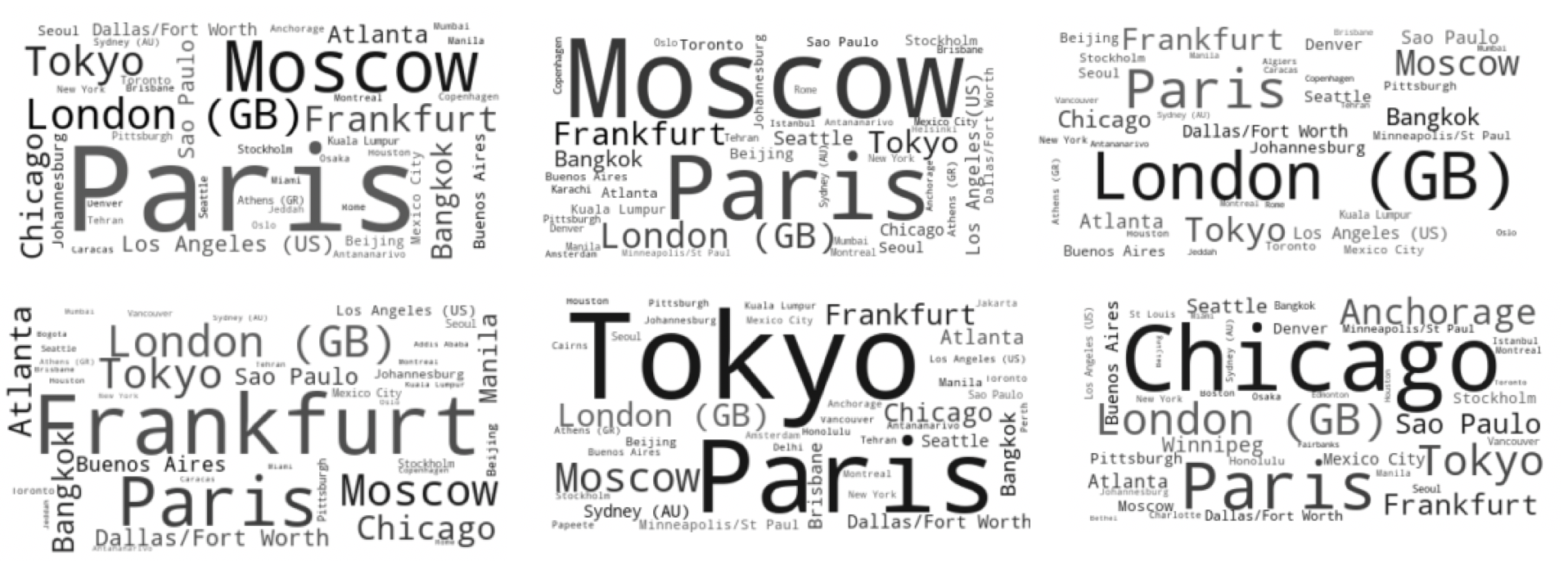
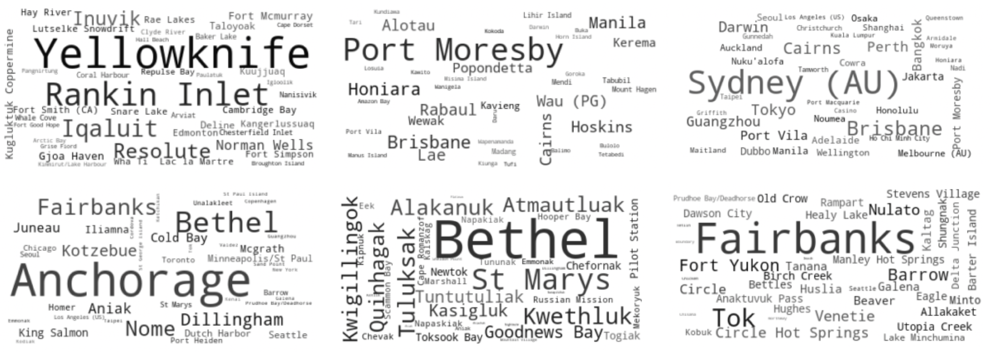
Figure 26: Top 12 community–trees on the air route network; first 6 trees reflect the hub of major global airports centered at different cities; tree 7 contains remote regional airports in the Northwest Territories province of Canada; tree 8 contains remote regional airports in southeast Asian Pacific islands; tree 9 contains Australia/Southeast Asia airports; tree 10 contains Alaskan airports while tree 11 and 12 contain western Alaskan and Northern Alaskan airports respectively.

S5.3 Additional clusters for statistician co-authorship network

In this section, we give 18 additional clusters discovered on the statistican co-authorship network in Figure 27, expanding the results given in Section 6.5 of the main paper.

(a) Bayesian

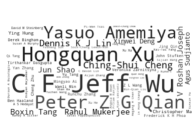
(b) Experimental design

(c) Biostat/Survey

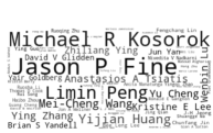
(d) Biostat

(e) Survey

(f) Causal

(g) Econometrics

(h) High dimensional

(i) High dimensional

(j) Theory

(k) Empirical likelihood/Inference

(l) High dim/Multivariate

(m) Sequential

(n) Spatial/Image

(o) Dimensionality reduction

(p) Time series

(q) Shape constrained

(r) Theory

Figure 27: Additional clusters from the statistician co-authorship network. We hand label a subset.

S5.4 Sampler diagnostic information

In this section, we give detailed sampler diagnostic information of the Gibbs sampling algorithm proposed in Section 4. We use a simulation setting where we generate a PAPER network with $n=2000$ nodes and $m=4000$ edges with $K=1$ and we also use the statistician co-authorship network analyzed in Section 6.5, which has $n=2263$ nodes and $m=4388$ edges.

Recall that our Gibbs sampler produces a sequence of samples of a spanning tree $\tilde{\bm{t}}_{n}^{(j)}$ and ordering $\pi^{(j)}$ for $j=1,2,\ldots,J$ where $J$ is the number of Gibbs outer iterations. We use $\tilde{\bm{t}}_{n}^{(j)}$ to compute the ”sampled” posterior root probability $Q^{(j)}(\cdot)=\mathbb{P}(\Pi_{1}=\cdot\,|\,\tilde{\bm{T}}_{n}=\tilde{\bm{t}}_{n}^{(j)})$. For the simulation setting, we then construct trace plot and auto-correlation plot based on the sequence $\{Q^{(j)}(\text{true root})\}_{j=1}^{J}$. For the statistician co-authorship network, we use construct the plots based on $\{Q^{(j)}(\text{ Raymond Carroll })\}_{j=1}^{J}$. Figures 28(a), 28(b), 28(c), and 28(d) suggest that the sampler is able to converge to the stationary distribution and has no significant autocorrelation.

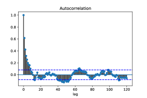
(a) ACF plot for a simulated network

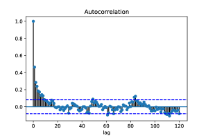
(b) ACF plot for the co-authorship network

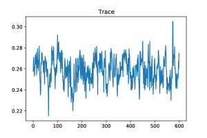
(c) Trace plot for a simulated network

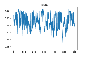
(d) Trace plot for the co-authorship network

Figure 28:

As described in Section S3.4, to assess convergence, we run two parallel chains $A$ and $B$ with corresponding posterior root probability estimates $Q^{A(1:J)}(\cdot)=\frac{1}{J}\sum_{j=1}^{J}Q^{A(j)}(\cdot)$ and $Q^{B(1:J)}(\cdot)=\frac{1}{J}\sum_{j=1}^{J}Q^{A(j)}(\cdot)$. We then compute the Hellinger distance $d_{\text{H}}(Q^{A(1:J)},Q^{B(1:J)})$ and increase $J$ until the distance is small enough. In Figures 29(a) and 29(b), we show that $d_{\text{H}}(Q^{A(1:J)},Q^{B(1:J)})$ indeed converges to 0 quickly as $J$ increases. We emphasize that the chains $A$ and $B$ are initialized with a uniformly random spanning tree and a uniformly random ordering on that tree so that the initialization is guaranteed to be overdispersed.

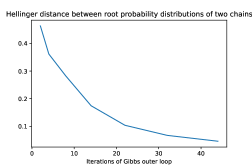
(a) Hellinger distance between the root probability distributions of two chains on a simulated network.

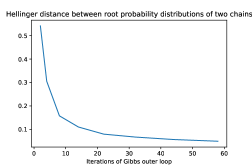
(b) Hellinger distance between the root probability distributions of two chains on the co-authorship network.

Figure 29:

References

- (1)
- Abbe (2017) Abbe, E. (2017). Community detection and stochastic block models: recent developments, The Journal of Machine Learning Research 18(1): 6446–6531.
- Adamic and Glance (2005) Adamic, L. A. and Glance, N. (2005). The political blogosphere and the 2004 us election: divided they blog, Proceedings of the 3rd international workshop on Link discovery, pp. 36–43.
- Addario-Berry and Eslava (2018) Addario-Berry, L. and Eslava, L. (2018). High degrees in random recursive trees, Random Structures & Algorithms 52(4): 560–575.
- Aiello et al. (2000) Aiello, W., Chung, F. and Lu, L. (2000). A random graph model for massive graphs, Proceedings of the thirty-second annual ACM symposium on Theory of computing, pp. 171–180.
- Albert et al. (1999) Albert, R., Jeong, H. and Barabási, A.-L. (1999). Diameter of the world-wide web, Nature 401(6749): 130–131.
- Aldous (1990) Aldous, D. J. (1990). The random walk construction of uniform spanning trees and uniform labelled trees, SIAM Journal on Discrete Mathematics 3(4): 450–465.
-
Amini et al. (2013)
Amini, A. A., Chen, A., Bickel, P. J. and Levina, E. (2013).
Pseudo-likelihood methods for community detection in large sparse
networks, Ann. Statist. 41(4): 2097–2122.
https://doi.org/10.1214/13-AOS1138 - Athreya et al. (2017) Athreya, A., Fishkind, D. E., Tang, M., Priebe, C. E., Park, Y., Vogelstein, J. T., Levin, K., Lyzinski, V. and Qin, Y. (2017). Statistical inference on random dot product graphs: a survey, The Journal of Machine Learning Research 18(1): 8393–8484.
- Banerjee and Bhamidi (2020) Banerjee, S. and Bhamidi, S. (2020). Root finding algorithms and persistence of jordan centrality in growing random trees, arXiv preprint arXiv:2006.15609 .
- Banerjee and Huang (2021) Banerjee, S. and Huang, X. (2021). Degree centrality and root finding in growing random networks, arXiv preprint arXiv:2105.14087 .
- Barabási (2016) Barabási, A.-L. (2016). Network science, Cambridge university press.
- Barabási and Albert (1999) Barabási, A.-L. and Albert, R. (1999). Emergence of scaling in random networks, Science 286(5439): 509–512.
- Bhamidi (2007) Bhamidi, S. (2007). Universal techniques to analyze preferential attachment trees: Global and local analysis.
- Bloem-Reddy et al. (2018) Bloem-Reddy, B., Foster, A., Mathieu, E. and Teh, Y. W. (2018). Sampling and inference for beta neutral-to-the-left models of sparse networks, Proceedings of UAI 2018 .
- Bloem-Reddy and Orbanz (2018) Bloem-Reddy, B. and Orbanz, P. (2018). Random-walk models of network formation and sequential monte carlo methods for graphs, Journal of the Royal Statistical Society: Series B (Statistical Methodology) 80(5): 871–898.
- Bollobás et al. (2001) Bollobás, B., Riordan, O., Spencer, J. and Tusnády, G. (2001). The degree sequence of a scale-free random graph process, Random Structures & Algorithms 18(3): 279–290.
- Briend et al. (2022) Briend, S., Calvillo, F. and Lugosi, G. (2022). Archaeology of random recursive dags and cooper-frieze random networks, arXiv preprint arXiv:2207.14601 .
- Broder (1989) Broder, A. (1989). Generating random spanning trees, 30th Annual Symposium on Foundations of Computer Science .
- Bubeck, Devroye and Lugosi (2017) Bubeck, S., Devroye, L. and Lugosi, G. (2017). Finding Adam in random growing trees, Random Structures & Algorithms 50(2): 158–172.
- Bubeck, Eldan, Mossel and Rácz (2017) Bubeck, S., Eldan, R., Mossel, E. and Rácz, M. Z. (2017). From trees to seeds: on the inference of the seed from large tree in the uniform attachment model, Bernoulli 23(4A): 2887–2916.
- Bubeck et al. (2015) Bubeck, S., Mossel, E. and Rácz, M. Z. (2015). On the influence of the seed graph in the preferential attachment model, IEEE Transactions on Network Science and Engineering 2(1): 30–39.
- Callaway et al. (2000) Callaway, D. S., Newman, M. E., Strogatz, S. H. and Watts, D. J. (2000). Network robustness and fragility: Percolation on random graphs, Physical review letters 85(25): 5468.
- Cantwell et al. (2019) Cantwell, G. T., St-Onge, G. and Young, J.-G. (2019). Recovering the past states of growing trees, arXiv preprint arXiv:1910.04788 .
- Cantwell et al. (2021) Cantwell, G. T., St-Onge, G. and Young, J.-G. (2021). Inference, model selection, and the combinatorics of growing trees, Physical Review Letters 126(3): 038301.
- Crane (2016) Crane, H. (2016). The ubiquitous Ewens sampling formula, Statistical Science 31(1): 1–39.
- Crane and Xu (2021) Crane, H. and Xu, M. (2021). Inference on the history of a randomly growing tree, Journal of Royal Statistical Society, series B (to appear.).
- Dereich and Mörters (2009) Dereich, S. and Mörters, P. (2009). Random networks with sublinear preferential attachment: degree evolutions, Electronic Journal of Probability 14: 1222–1267.
- Devroye and Reddad (2018) Devroye, L. and Reddad, T. (2018). On the discovery of the seed in uniform attachment trees, arXiv preprint arXiv:1810.00969 .
- Diaconis and Janson (2007) Diaconis, P. and Janson, S. (2007). Graph limits and exchangeable random graphs, arXiv preprint arXiv:0712.2749 .
- Drmota (2009) Drmota, M. (2009). Random trees: an interplay between combinatorics and probability, Springer Science & Business Media.
- Fioriti et al. (2014) Fioriti, V., Chinnici, M. and Palomo, J. (2014). Predicting the sources of an outbreak with a spectral technique, Applied Mathematical Sciences 8: 6775–6782.
- Galashin (2013) Galashin, P. (2013). Existence of a persistent hub in the convex preferential attachment model, arXiv preprint arXiv:1310.7513 .
- Gao et al. (2015) Gao, C., Lu, Y. and Zhou, H. H. (2015). Rate-optimal graphon estimation, The Annals of Statistics 43(6): 2624–2652.
- Guimera et al. (2005) Guimera, R., Mossa, S., Turtschi, A. and Amaral, L. N. (2005). The worldwide air transportation network: Anomalous centrality, community structure, and cities’ global roles, Proceedings of the National Academy of Sciences 102(22): 7794–7799.
- Hens et al. (2012) Hens, N., Calatyud, L., Kurkela, S., Tamme, T. and Wallinga, J. (2012). Robust reconstruction and analysis of outbreak data: influenza a(h1n1)v transmission in a school-based population, American Journal of Epidemiology 176(3): 196–203.
- Hoff et al. (2002) Hoff, P. D., Raftery, A. E. and Handcock, M. S. (2002). Latent space approaches to social network analysis, Journal of the american Statistical association 97(460): 1090–1098.
- Jeong et al. (2001) Jeong, H., Mason, S. P., Barabási, A.-L. and Oltvai, Z. N. (2001). Lethality and centrality in protein networks, Nature 411(6833): 41.
- Ji and Jin (2016) Ji, P. and Jin, J. (2016). Coauthorship and citation networks for statisticians, The Annals of Applied Statistics 10(4): 1779–1812.
- Jiang et al. (2016) Jiang, J., Wen, S., Yu, S., Xiang, Y. and Zhou, W. (2016). Identifying propagation sources in networks: State-of-the-art and comparative studies, IEEE Communications Surveys & Tutorials 19(1): 465–481.
- Jin (2015) Jin, J. (2015). Fast community detection by SCORE, The Annals of Statistics 43(1): 57–89.
- Karrer and Newman (2011) Karrer, B. and Newman, M. E. (2011). Stochastic blockmodels and community structure in networks, Physical review E 83(1): 016107.
- Khim and Loh (2017) Khim, J. and Loh, P.-L. (2017). Confidence sets for the source of a diffusion in regular trees, IEEE Transactions on Network Science and Engineering 4(1): 27–40.
- Knuth (1997) Knuth, D. E. (1997). The Art of Computer Programming: Volume 1: Fundamental Algorithms, Addison-Wesley Professional.
- Kolaczyk (2009) Kolaczyk, E. D. (2009). Statistical Analysis of Network Data: Methods and Models, Springer Series in Statistics.
- Leskovec et al. (2009) Leskovec, J., Lang, K. J., Dasgupta, A. and Mahoney, M. W. (2009). Community structure in large networks: Natural cluster sizes and the absence of large well-defined clusters, Internet Mathematics 6(1): 29–123.
- Lugosi et al. (2019) Lugosi, G., Pereira, A. S. et al. (2019). Finding the seed of uniform attachment trees, Electronic Journal of Probability 24.
- Mislove et al. (2007) Mislove, A., Marcon, M., Gummadi, K. P., Druschel, P. and Bhattacharjee, B. (2007). Measurement and Analysis of Online Social Networks, Proceedings of the 5th ACM/Usenix Internet Measurement Conference (IMC’07), San Diego, CA.
- Na and Rapoport (1970) Na, H. S. and Rapoport, A. (1970). Distribution of nodes of a tree by degree, Mathematical Biosciences 6: 313–329.
- Peköz et al. (2014) Peköz, E. A., Röllin, A. and Ross, N. (2014). Joint degree distributions of preferential attachment random graphs, arXiv preprint arXiv:1402.4686 .
- Pollard (2002) Pollard, D. (2002). A user’s guide to measure theoretic probability, number 8, Cambridge University Press.
-
Rossi and Ahmed (2015)
Rossi, R. A. and Ahmed, N. K. (2015).
The network data repository with interactive graph analytics and
visualization, AAAI.
http://networkrepository.com - Shah and Zaman (2011) Shah, D. and Zaman, T. (2011). Rumors in a network: Who’s the culprit?, IEEE Transactions on information theory 57(8): 5163–5181.
- Shelke and Attar (2019) Shelke, S. and Attar, V. (2019). Source detection of rumor in social network–a review, Online Social Networks and Media 9: 30–42.
- Sheridan et al. (2008) Sheridan, P., Yagahara, Y. and Shimodaira, H. (2008). A preferential attachment model with poisson growth for scale-free networks, Annals of the institute of statistical mathematics 60(4): 747–761.
- Sheridan et al. (2012) Sheridan, P., Yagahara, Y. and Shimodaira, H. (2012). Measuring preferential attachment in growing networks with missing-timelines using markov chain monte carlo, Physica A: Statistical Mechanics and its Applications 391(20): 5031–5040.
- Sreedharan et al. (2019) Sreedharan, J. K., Magner, A., Grama, A. and Szpankowski, W. (2019). Inferring temporal information from a snapshot of a dynamic network, Scientific reports 9(1): 1–10.
- Van Der Hofstad (2016) Van Der Hofstad, R. (2016). Random graphs and complex networks, Vol. 1, Cambridge university press.
- Wade and Ghahramani (2018) Wade, S. and Ghahramani, Z. (2018). Bayesian cluster analysis: Point estimation and credible balls (with discussion), Bayesian Analysis 13(2): 559–626.
- West (1992) West, M. (1992). Hyperparameter estimation in Dirichlet process mixture models, Duke University ISDS Discussion Paper# 92-A03.
- Wilson (1996) Wilson, D. B. (1996). Generating random spanning trees more quickly than the cover time, Proceedings of the twenty-eighth annual ACM symposium on Theory of computing, pp. 296–303.
- Xie and Xu (2019) Xie, F. and Xu, Y. (2019). Optimal bayesian estimation for random dot product graphs, arXiv preprint arXiv:1904.12070 .
- Xu et al. (2018) Xu, M., Jog, V. and Loh, P.-L. (2018). Optimal rates for community estimation in the weighted stochastic block model, Annals of Statistics, Accepted, to appear .
- Young et al. (2019) Young, J.-G., St-Onge, G., Laurence, E., Murphy, C., Hébert-Dufresne, L. and Desrosiers, P. (2019). Phase transition in the recoverability of network history, Physical Review X 9(4): 041056.
- Zachary (1977) Zachary, W. W. (1977). An information flow model for conflict and fission in small groups, Journal of anthropological research 33(4): 452–473.