The three-year shear catalog of the Subaru Hyper Suprime-Cam SSP Survey

Abstract

We present the galaxy shear catalog that will be used for the three-year cosmological weak gravitational lensing analyses using data from the Wide layer of the Hyper Suprime-Cam (HSC) Subaru Strategic Program (SSP) Survey. The galaxy shapes are measured from the $i$-band imaging data acquired from 2014 to 2019 and calibrated with image simulations that resemble the observing conditions of the survey based on training galaxy images from the Hubble Space Telescope in the COSMOS region. The catalog covers an area of 433.48 deg² of the northern sky, split into six fields. The mean $i$-band seeing is 0.59 arcsec. With conservative galaxy selection criteria (e.g., $i$-band magnitude brighter than 24.5), the observed raw galaxy number density is 22.9 arcmin^-2, and the effective galaxy number density is 19.9 arcmin^-2. The calibration removes the galaxy property-dependent shear estimation bias to a level: $|\delta m|<9\times 10^{-3}$. The bias residual $\delta m$ shows no dependence on redshift in the range $0<z\leq 3$. We define the requirements for cosmological weak lensing science for this shear catalog, and quantify potential systematics in the catalog using a series of internal null tests for systematics related to point-spread function modelling and shear estimation. A variety of the null tests are statistically consistent with zero or within requirements, but (i) there is evidence for PSF model shape residual correlations; and (ii) star-galaxy shape correlations reveal additive systematics. Both effects become significant on $>1$ degree scales and will require mitigation during the inference of cosmological parameters using cosmic shear measurements.

1 Introduction

In the current standard structure formation paradigm (the $\Lambda$CDM model), dark matter and dark energy constitute a large fraction (about 95%) of the total energy density of the Universe (Planck Collaboration et al., 2020; Suzuki et al., 2012; Mandelbaum et al., 2013). Unveiling the nature of these two mysterious components, dark matter and dark energy, is one of the most tantalizing problems in cosmology and physics, and is one of the major goals for ongoing and upcoming wide-area galaxy surveys (see Weinberg et al. 2013 for a review). Among different cosmological probes, weak gravitational lensing provides us with a unique means of measuring matter distribution (including dark matter) in the universe (e.g. Miyazaki et al., 2018a), via the deflection of light due to the gravitational potential field in cosmic structures along the line-of-sight, which both magnifies and distorts galaxy shapes – the so-called cosmological weak lensing or cosmic shear (see Mandelbaum 2018 for a review). Since the initial detections of cosmic shear (Bacon et al., 2000; Van Waerbeke et al., 2000; Rhodes et al., 2001), weak lensing now has become one of the indispensable methods for precision cosmology.

The standard method to measure cosmic shear is based on the auto-correlation of galaxy shape distortions. When combined with photometric redshift information of individual galaxies via their multi-color photometry, known as “cosmic shear tomography”, the cosmic shear correlation functions are very powerful at measuring scale-dependent amplitudes and time evolution of matter clustering in large-scale structure. These measurements are in turn used to place powerful constraints on the present-day amplitudes of matter fluctuations, the matter density (mostly dark matter), and the nature of dark energy (see e.g., Hildebrandt et al., 2017a; Troxel et al., 2018; Hikage et al., 2019a; Hamana et al., 2020; Asgari et al., 2021; Secco et al., 2021; Amon et al., 2021). The galaxy-shear cross-correlation function, or galaxy-galaxy weak lensing, can be combined with galaxy clustering to observationally disentangle galaxy bias uncertainty and thus obtain useful constraints on the cosmological parameters (see e.g., Mandelbaum et al., 2013; More et al., 2015; Abbott et al., 2018; Heymans et al., 2021; Miyatake et al., 2021). Furthermore, when combined with the redshift-space distortion effect due to peculiar velocities of lens galaxies, properties of gravity (i.e. gravity theory) on cosmological scales can be tested (e.g. Blake et al., 2016; Alam et al., 2017).

The current generation wide-area multi-color surveys that have weak lensing among their primary science cases are: the Kilo-Degree Survey (KiDS; de Jong et al., 2013), the Dark Energy Survey (DES; Dark Energy Survey Collaboration et al., 2016), and the survey that is the subject of this paper: the Hyper Suprime-Cam survey (HSC; Miyazaki et al., 2018b; Aihara et al., 2018b). The unique aspect of the HSC survey is its combination of depth and high-resolution imaging that gives it a longer redshift baseline than the others. Hence the weak lensing information obtained from the HSC survey is complementary to those of the KiDS and DES surveys that probe weak lensing effects at lower redshifts, but over a wider area than the current HSC survey does. In addition, the excellent image quality in HSC should enable us to pin down sources of systematic uncertainties in weak lensing shear. In the coming decade, three ultimate imaging surveys will become available and promise to place further stringent constraints on cosmological parameters including the nature of dark energy. Those are the Euclid satellite mission (Laureijs et al., 2011), Vera C. Rubin Observatory’s Legacy Survey of Space and Time (LSST; Ivezić et al., 2019), and the Nancy Grace Roman Space Telescope (Spergel et al., 2015). Since the HSC data is the deepest among the ongoing surveys, the HSC survey can be considered as a precursor survey for LSST since they are both ground-based data and share similarities in the depth and image quality. Hence it is important and timely to assess and figure out whether the quality and issues of the HSC data can meet requirements to use the weak lensing measurements for cosmology, compared to the statistical errors of the current HSC data.

However, weak lensing shear is a tiny effect typically causing one percent ellipticities in the observed galaxy images, which are smaller than the root-mean-square (RMS) of intrinsic galaxy shapes. Thus the shear is only measurable in a statistical sense. Hence an accurate weak lensing measurement requires exquisite characterization of individual galaxy images as well as control and calibrations of all observational effects such as atmospheric effects (point-spread function and background noise) and the detector noise. It is important to ensure that residual systematic errors are well below the statistical error floor so that any physical constraints obtained from the weak lensing measurements are not biased. Observationally there are several sources of systematic effects inherent in characterizing galaxy shapes, even in a statistical sense: (i) “noise bias” due to the non-linear impact of noise on shear estimation (Refregier et al., 2012; Zhang & Komatsu, 2011); (ii) “model bias” due to imperfect assumptions about galaxy morphology (e.g., Bernstein, 2010); (iii) “weight bias” caused by shear-dependent weighting (e.g., Fenech Conti et al., 2017); (iv) “selection bias” originating from an improper treatment of selection effects around cuts (e.g., Mandelbaum et al., 2005); (v) systematics related to blending of galaxy light profiles (e.g., Li et al., 2018; Sheldon et al., 2020); (vi) mis-estimation of the point-spread function (PSF; e.g., Lu et al., 2017); and (vii) other systematics from detector non-idealities – e.g., “tree rings”, “edge distortions” (Plazas et al., 2014), and brighter-fatter effects (Antilogus et al., 2014) – and from the atmosphere – e.g., differential chromatic refraction (DCR; Plazas & Bernstein, 2012). There are other astrophysical uncertainties such as photometric redshift errors, intrinsic alignments of galaxy shapes and the impact of baryonic effects (Mandelbaum, 2018). In this paper we focus on the observational effects in galaxy shape characterizations for weak lensing measurements.

Because of the systematics mentioned above, it is necessary to validate the shear catalog generation pipeline using image simulations. To develop simulations representative of the real data, the issue that arises here is how to maximally represent the real observational conditions and the galaxy properties in the HSC data. Much effort has been made to produce simulations that faithfully represent the image characteristics that affect shear estimation (Mandelbaum et al., 2018b; Kannawadi et al., 2019; MacCrann et al., 2020). Shear estimators must be calibrated if the biases discovered with image simulations exceed the systematic error requirements of the weak lensing survey. In addition, internal “null tests” related to galaxy and star shapes within the shear catalog are important to uncover the signatures of the aforementioned systematics (e.g., Mandelbaum et al., 2018a; Giblin et al., 2021; Gatti et al., 2021).

In this paper, we describe the process to generate the three-year shear catalog for weak lensing statistics from the HSC-SSP S19A internal data release (released in September 2019). First, we measure galaxy shapes using the re-Gaussianization method (reGauss; Hirata & Seljak, 2003), and calibrate the shear estimation bias using HSC-like galaxy image simulations following the formalism of Mandelbaum et al. (2018b). We then calculate the requirements for cosmological analysis based on the survey parameters. We subsequently proceed with data quality control with “null tests” on the catalog following Mandelbaum et al. (2018a), which include tests related to PSF modelling, cross-correlations of galaxy shapes with random positions, star positions and star shapes, and tests related to weak lensing mass maps.

The structure of the paper is outlined as follows. In Section 2, we present the S19A internal HSC data release, and outline the updates in the pipeline used to process the S19A data. In Section 3, we calibrate reGauss galaxy shapes with realistic image simulations and characterize the three-year HSC shear catalog. In Section 4, we define the requirements for the shape catalog on the PSF modelling and shear inference to ensure that the three-year weak lensing science is minimally affected by the systematics we listed above. In Section 5, we perform various systematic tests associated to the PSF modelling to ensure the quality of PSF reconstruction and correction. Finally, we conduct null tests on the shear catalog in Section 6, and summarize in Section 7.

2 HSC Data and Pipeline

The HSC instrument (Furusawa et al., 2018a; Miyazaki et al., 2018c) is a wide-field optical imager mounted on the $8.2$-meter Subaru Telescope. The HSC-SSP (Aihara et al., 2018b) is a deep multi-band imaging survey with a target area of $1400$ $\rm{deg}^{2}$ on the northern sky. The HSC pipeline (Bosch et al., 2018) is a fork of Rubin’s LSST Science Pipelines (Bosch et al., 2019); the fork is being developed to process the data from the HSC-SSP survey, while an updated version of Rubin’s LSST Science Pipelines will be used for LSST.

The first public data release of HSC data (PDR1, Aihara et al., 2018a) was based on the S15B internal data release (released in January 2016) and included images and catalogs processed with $\texttt{hscPipe}~{}{\rm v}4$ (Bosch et al., 2018). The first-year HSC shear catalog (Mandelbaum et al., 2018a) was based on the S16A internal data release (released in August 2016) and was also processed with $\texttt{hscPipe}~{}{\rm v}4$.

The second public data release (PDR2) of images and catalogs was based on the S18A internal data release (released in June 2018) processed with $\texttt{hscPipe}~{}{\rm v}6$ (Aihara et al., 2019). There were major updates on the pipeline from $\texttt{hscPipe}~{}{\rm v}4$ to $\texttt{hscPipe}~{}{\rm v}6$ as summarized in Aihara et al. (2019).

The shear catalog introduced in this paper is based on the S19A internal data release (released in September 2019) acquired from March 2014 to April 2019. The S19A images are processed with $\texttt{hscPipe}~{}{\rm v}7$. Here we briefly summarize the new features of $\texttt{hscPipe}~{}{\rm v}7$ updated from $\texttt{hscPipe}~{}{\rm v}4$ that are important for weak lensing measurements. In addition, we summarize the changes in the observing strategy. As our first-year shear catalog helped to identify areas where progress was needed in the image processing pipeline, we expect this paper to provide a snapshot of the current state of the software pipeline, and to help in identifying further areas for progress.

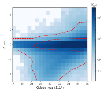
Figure 1: $2$D histogram of the $i$-band magnitude difference and the S19A CModel magnitude. The magnitude difference ($\Delta$mag) is defined as the S19A CModel minus the S16A CModel magnitude. Galaxies are matched between S19A and S16A within the first-year HSC weak lensing full depth full color region (Mandelbaum et al., 2018a) within $0\farcs 5$. The contours are for galaxy numbers of $10^{2}$ and $10^{5}$, respectively.

2.1 Improvements in PSF modelling

The HSC pipeline uses a repackaged version of PSFEx (Bertin, 2011) to estimate point-spread function (PSF) models on single exposures, and the PSF models on coadds are estimated using the PSF models from each exposure, while accounting for the warping kernel used for image coaddition (Bosch et al., 2018).

The PSFs on single exposures are modelled by PSFEx using a pixellated basis function, and in principle the over-sampled PSF model can be shifted by sub-pixel offsets using sinc interpolation. However, the Lanczos kernels, employed by the original version of PSFEx in $\texttt{hscPipe}~{}{\rm v}4$ to approximate the sinc kernel caused problems for images with the “very best seeing”. As shown in Fig. 9 of Aihara et al. (2019), the sizes of PSF models are less than the sizes of observed stars by $0.4$% for regions with seeing FWHM of around $0\farcs 5$.

For the second data release, as described in Section 4.6 in Aihara et al. (2019), the pipeline resampled the PSF models by interpreting the PSF models as a constant over each sub-pixel, rather than a continuous function sampled at the pixel center. This mitigated the PSF model errors for images with the “very best seeing”, reducing the fractional size residual between PSF models and observed stars from $\sim 0.4$% to $\sim 0.1$%. This new interpolation scheme is subsequently applied in the S19A image processing.

2.2 Improvements to the warping kernel

In the coaddition process, each single CCD image is convolved with a warping kernel to transform discrete (pixellated) images into continuous images. The warped images are subsequently resampled onto a common coordinate system.

For the data releases before S19A, a third-order Lanczos kernel was used to warp CCD images before coadding the images. As reported in Section 6.4 of Aihara et al. (2019), the sizes of observed PSFs on coadds are 0.4% larger than that of reconstructed PSF models. Aihara et al. (2019) showed that the amplitude of PSF size residuals decreases when the order of the warping kernel is increased to fifth-order.

A systematic bias on galaxy shape measurements stemming from such a $0.4\%$ fractional size residual in PSF size was not significant when compared to the first-year weak lensing science requirements (Mandelbaum et al., 2018a). However, for the three-year weak lensing shear catalog, the survey area has significantly increased and the science requirements are consequently much tighter (see Section 4). Therefore, we switch to using the fifth-order Lanczos warping kernel. The tests quantifying PSF model fidelity are presented in Section 5.

2.3 Background subtraction

For the HSC first-year data release (DR1), the pipeline performed a local background subtraction at the single exposure level with a $128\times 128$ ($\sim 22\times 22\arcsec$) pixel-mesh on each CCD individually. To estimate the sky background, the pipeline averaged pixels in each pixel-mesh ignoring detected pixels. Then the background was modelled with $2$D Chebyshev polynomials. After coadding single exposures into coadds, the pipeline performed a background subtraction with a larger ($\rm 4k\,\times 4k$, or $11\arcmin\times 11\arcmin$) pixel-mesh (see Bosch et al. 2018 for more details) after masking out the detections on coadds. This background subtraction scheme was found to cause over-subtraction around bright objects since it subtracts flux from the wings of bright extended objects along with the sky background (Bosch et al., 2018).

In the second-year data release (DR2), the background subtraction scheme was updated as follows: At the single exposure level, the pipeline performed a global joint estimation of the background using all the CCDs across the focal plane to reduce the aforementioned over-subtraction. In addition, the pipeline estimates and subtracts the “sky frame” — the mean response of the instrument to the sky for a particular filter. The sky frame is estimated from a clipped-mean of the pixel-mesh with detected objects masked out from many observations with large dithers (see Aihara et al. 2019 for more details). The pipeline then applied the same background subtraction scheme as before on coadds. This background subtraction scheme preserves the extended wings of bright objects; however, it influences the CModel measurement, which measures the flux by fitting the galaxy’s surface brightness profile with an exponential and a de Vaucouleurs (de Vaucouleurs, 1948) profile separately. The preserved wings of neighboring bright objects and background residuals lead to larger estimates of galaxy CModel radii and increase the CModel flux estimates, especially for faint sources near bright objects.

With the intent to mitigate the under-subtraction problem and improve the performance of CModel measurements, a local background subtraction with a $128\times 128$ (local) pixel-mesh is applied on coadds in S19A. In addition, we use an improved global background subtraction scheme during single exposure image processing to remove global sky background and “sky frame” (see Aihara et al. 2021 for more details). This background subtraction scheme reduces the aforementioned background residuals caused by the background subtraction scheme in the second data release. However, the CModel magnitude estimates in S19A are still brighter than in S16A due to the influence of background residuals in S19A. As illustrated by the $2$D histogram of the $i$-band CModel magnitude difference between S19A and S16A as a function of the S19A magnitude in Fig. 1, the histogram is skewed to negative $\Delta$mag. Fig. 1 indicates that objects appear brighter in S19A. In addition, we find that the galaxies with negative magnitude difference cluster around bright objects (e.g., bright stars and bright galaxies). The details are summarized in the HSC third data release paper (Aihara et al., 2021).

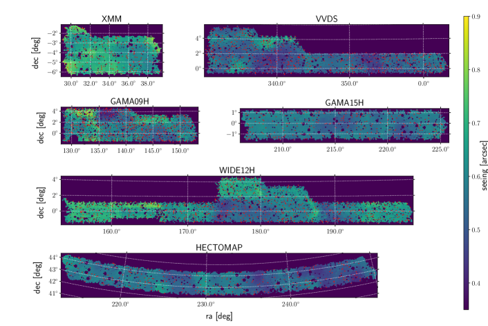
Figure 2: Map of the $i$-band PSF FWHM across each field. The red dots are the sampling positions for PSFs and noise properties that will be used in the HSC-like image simulation in Section 3.2. The mean seeing over all of the fields is $0\farcs 59$. The circular region centered near (RA=$130\fdg 43$, DEC=$-1\fdg 02$) of the GAMA09H field is masked out due to the tracking error on the exposure visit 104934.

2.4 Bright star mask

In this section we describe how bright star masks are applied to the weak lensing shear catalog. Those who are interested in more details of the bright star mask construction, please refer to the PDR3 paper (Aihara et al., 2021). The S19A bright star masks are created using the Gaia second data release (Gaia Collaboration et al., 2018) as a reference catalog in which Gaia magnitudes are converted to HSC magnitudes. The star masks are defined for stars brighter than 18th magnitude and for different types of artifacts; halo, ghost, blooming, scratch, and dip. The scratch mask is designed to mask vertical stripes around bright stars in long-wavelength bands (e.g., $y$-band and NB1010-band) due to the channel-stop, if the CCD is optically thin with respect to the wavelength (for more details, see Aihara et al., 2021). Since the shear catalog is based on $i$-band images, the scratch mask is not considered for the shear catalog. The dip mask is for masking over-subtracted region in the vicinity of a star due to the local background subtraction. The over-subtraction affects the number count of source galaxies but does not have significant influence on shape estimation. In addition, applying the dip mask reduces the area significantly. Therefore, the dip mask is not considered for the shear catalog. The shear estimation near stars is tested in Section 6.2.

For the weak lensing shear catalog, we adopt the star masks for halo, ghost, and blooming. The flags used for selection are summarized in Table 1. The halo mask masks an extended smooth halo around a star whose size depends on the brightness of a star. To define the halo mask, a median radial profile was computed for stars within a magnitude bin, and the mask was defined up to the scale where the profiles goes down to the background level. The size of halo mask decreases as a function of magnitude. The ghost mask is defined using the median radial profile and a cross-correlation with objects around bright stars where ghost edges induce spurious detection of objects. The radius of ghost mask is $350\arcsec$ for stars brighter than 7th magnitude and $160\arcsec$ for stars between $7$th and $9$th magnitude. The exact size and shape of ghost depends on the telescope boresight and a bright star, and fake objects outside the mask are found in some cases. To deal with such cases, we adopt the ghost mask with 50% larger than the standard size defined above. The blooming appears parallel to the channel-stop of a CCD, which is always horizontal in the image because rotational dithers are not performed in the SSP survey. The scale of the blooming feature depends on the star brightness and positions on the CCD inputs, the maximum of which is $\sim 10\arcmin$. To define the blooming mask, the cross-correlation measurement was performed along the horizontal and vertical directions, and a detection excess along the horizontal direction was considered a blooming. The blooming mask is defined as a function of stellar magnitude.

Table 1: Flags of bright star masks considered in our shear catalog. Objects flagged as True by any one of the masks are removed.

Mask Flag	Meaning
i$\_$mask$\_$brightstar$\_$ghost15	Ghost
i$\_$mask$\_$brightstar$\_$halo	Halo
i$\_$mask$\_$brightstar$\_$blooming	Blooming

2.5 Observing strategy

The observing strategy underwent a couple of changes in order to increase the effective survey completion speed. Firstly, the number of dithers per pointing in the $i$-, $z$-, and $y$-bands were reduced from $6$ to $5$ since November 2018. This change results in a survey depth that is shallower by $0.1$ magnitudes on average. The nominal $5\sigma$ depth for point sources in $i$-band was $26.2$ for PDR2 based on S18A (see Table 2 of Aihara et al., 2019). Our shear catalog only contains galaxies with $i$-band magnitudes brighter than $24.5$, and thus the change in depth is not expected to significantly affect the statistical properties of the shear catalog.

The original requirement on the seeing conditions for procuring $i$-band images was also relaxed from $0\farcs 7$ to $0\farcs 9$; this requirement is imposed using the on-site quick-look software (Furusawa et al., 2018b), which monitors the data quality with a lag of only a few minutes. Despite the fact that the requirement was relaxed, the mean $i$-band seeing for the entire three year data set used in this paper is $0\farcs 59$, similar to that of the first-year HSC shear catalog (Mandelbaum et al., 2018a). We look into the PSF model errors in the regions observed with 6 dithers and with 5 dithers in Section 5, the results of which do not show significant difference in the PSF model errors between the two observational strategies.

2.6 Full depth and full color cut

We restrict ourselves to regions that reach the approximate full depth of the survey in all five broadband filters ($grizy$), in order to achieve better uniformity of the shear estimation and photometric redshift quality across the survey as was also done in Mandelbaum et al. (2018a). This cut is imposed by requiring the average number of visits contributing to the coadds within HEALPix pixels (with $\rm{NSIDE}=1024$) to be $(g,r,i,z,y)\geq(4,4,5,5,5)$. Note that this is different from the requirement in the first-year shear catalog that was $(g,r,i,z,y)\geq(4,4,4,6,6)$. In the first-year shear catalog, some of the $i$-band visits with the “very best seeing” were removed because of the inability to model the PSFs, and thus the minimum number of $i$-band exposure was set to $4$ (Mandelbaum et al., 2018a). However, since the PSF determination in the HSC pipeline was improved as described in Section 2.1, such exposures are added back to the coadds. In addition, the $5$-dithering strategy was adopted in November 2018. We thus set the requirement on the minimum numbers of average input visits for $i$-band to 5. For the $z$- and $y$-bands, we set the requirement to 5 as well, following the change in dithering strategy.

As will be discussed in Section 5.2, we also remove a few regions with large average PSF size modelling errors. This PSF size modelling error cut reduces the survey area by $\sim 2.2\%$.

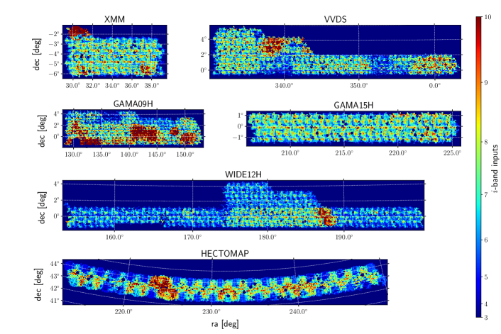
Figure 3: Number of input visits contributing to the coadds in the $i$-band across each field. The mean number of input visits is $6.95$ over all of the fields. The way the visits are tiled across each survey area results in the repeated pattern of overlap regions with number of inputs more than the typical value (see Aihara et al. (2018b) for the tiling strategy).

After these cuts, the total area of the catalog is $433.48~{}\mathrm{deg}^{2}$. The footprint of the galaxy catalog is divided into six observational fields, i.e., XMM, GAMA09H, WIDE12H, GAMA15H, VVDS, HECTOMAP, the areas of which are 33.17 $\mathrm{deg}^{2}$, 98.85 $\mathrm{deg}^{2}$, 121.32 $\mathrm{deg}^{2}$, 40.87 $\mathrm{deg}^{2}$, 96.18 $\mathrm{deg}^{2}$, and 43.09 $\mathrm{deg}^{2}$. Fig. 2 shows the $i$-band seeing map. Fig. 3 shows the map of the number of $i$-band visits contributing to the coadd. Fig. 4 shows the seeing histograms, and Fig. 5 shows the noise variance histograms.

3 Shear Catalog

In this section, we introduce the shear catalog measured from the HSC S19A $i$-band coadded images. We first review the shear estimation process in Section 3.1. In Section 3.2, we present the $i$-band image simulations used for the calibration of shear measurements. The selection criteria for the weak lensing shear catalog are presented in Section 3.3. We subsequently determine the intrinsic shape dispersion and the optimal weight for shear estimation in Section 3.4, calibrate the bias in the shear estimation in Section 3.5, and quantify the amplitude of the calibration bias residuals in Section 3.6. Selection bias is estimated and calibrated in Section 3.7. Finally, the shear catalog is characterized in Section 3.9 and our blinding strategy to avoid confirmation bias in weak lensing analyses is presented in Section 3.10.

3.1 Shear estimation

3.1.1 Detection, deblending and source replacement

In this subsection, we briefly summarize the processes of source detection, deblending and source replacement after coadding single exposures and background subtraction based on $\texttt{hscPipe}~{}{\rm v}7$.

The HSC pipeline (Bosch et al., 2018) performs a maximum-likelihood source detection with a $5\sigma$ threshold from the coadded images. Every peak detected is identified as a source and the connected nearby region above the threshold is identified as the footprint of the source detection.

For the case that a footprint contains multiple sources, these sources are taken as blended, and the HSC pipeline apportions the flux to these blended sources using the SDSS deblending algorithm (Lupton et al., 2001). This deblending algorithm takes each peak as a ‘child’ source of the ‘parent’ detection. A template for each ‘child’ is constructed with the assumption that each source has $180~{}\deg$ rotational symmetry around its detected peak. Then a scaling parameter is determined for each source by jointly fitting the templates to the blended image.

After deblending, the HSC pipeline performs source measurement (e.g., flux, size, and shape) on each source. During the deblending and measurement of one detection, the pipeline replaces the footprints of other sources with uncorrelated Gaussian noise.

3.1.2 Re-Gaussianization

Galaxy shapes are estimated with the GalSim (Rowe et al., 2015) implementation of the re-Gaussianization (reGauss) PSF correction method (Hirata & Seljak, 2003). This moments-based method has been developed and used extensively using data from the Sloan Digital Sky Survey (SDSS; Mandelbaum et al., 2005, 2013). The outputs of the reGauss estimator are the two components of the ellipticity of each galaxy:

$$(e_{1},e_{2})=\frac{1-(b/a)^{2}}{1+(b/a)^{2}}(\cos 2\phi,\sin 2\phi),$$ (1)

where $b/a$ is the axis ratio and $\phi$ is the position angle of the major axis with respect to sky coordinates (with north being $+y$ and east being $+x$). Another important output of the pipeline is the resolution factor $R_{2}$, which is defined for each galaxy using the trace of the second moments of the PSF ($T_{{\rm PSF}}$) and those of the observed galaxy image ($T_{{\rm gal}}$):

$$R_{2}=1-\frac{T_{{\rm PSF}}}{T_{{\rm gal}}}\,.$$ (2)

The resolution factor is used to quantify the extent to which the galaxy is resolved compared to the PSF.

For an isotropically-orientated galaxy ensemble distorted by a constant shear, the shear can be estimated with a weighted average of the ellipticity of all galaxies:

$$\hat{g}_{\alpha}=\frac{1}{2\mathcal{R}}\left\langle e_{\alpha}\right\rangle,$$ (3)

where the shear responsivity ($\mathcal{R}$) is the response of the average galaxy ellipticity to a small shear distortion (Kaiser et al., 1995; Bernstein & Jarvis, 2002), and $\alpha=1,2$ are the indices for the two components of the ellipticity. The inverse variance weights to be used while performing the ensemble average are the galaxy shape weights ($w_{i}$) defined as

$$w_{i}=\frac{1}{\sigma_{e;i}^{2}+e_{{\rm RMS};i}^{2}},$$ (4)

where $i$ is an index over galaxies, $\sigma_{e}$ is the per-component $1\sigma$ uncertainty of the shape estimation error due to photon noise, and $e_{\rm{RMS}}$ denotes the per-component root-mean-square (RMS) of the galaxy intrinsic ellipticity. The parameters $e_{\rm{RMS}}$ and $\sigma_{e}$ are modeled and estimated for each galaxy using image simulations, as will be discussed in Section 3.4. The responsivity for the source galaxy population is estimated as

$$\mathcal{R}=1-\frac{\sum_{i}w_{i}e^{2}_{{\rm RMS};i}}{\sum_{i}w_{i}}\,.$$ (5)

As the PSFs are nearly round, the responsivity for PSFs is approximately one, and the shear distortion for a PSF image is defined as $g_{{\rm PSF},\alpha}=e_{{\rm PSF},\alpha}/2$, where $e_{{\rm PSF},\alpha}$ are the two components ($\alpha=1,2$) of PSF ellipticity defined with the second moments of the PSF. We refer the reader to Section 5 for tests on PSF-related systematics.

3.1.3 Shear estimation bias

Since the reGauss algorithm is subject to certain forms of shear estimation bias (e.g., model bias, noise bias, and selection bias), in this section, we define the calibration parameters that will encapsulate those biases and review the calibrated form of the reGauss shear estimator. The relation between the estimated shear and the true shear at the individual galaxy level is quantified by

$$\hat{g}_{\alpha;i}=(1+m_{i})g_{\alpha;i}+a_{i}e_{\mathrm{PSF},\alpha;i}\,,$$ (6)

where $m_{i}$ is the multiplicative bias and $a_{i}$ is the fractional additive bias quantifying the fraction of the PSF anisotropy (ellipticity) that leaks into the shear estimation. Terms involving spin-$4$ quantities, which average to zero when averaging $\hat{g}_{\alpha;i}$ over all galaxies in the sample, are neglected. The two components of the additive bias are thus given by $c_{\alpha}\equiv ae_{\mathrm{PSF},\alpha}$. Here we neglect the additive bias that is independent of PSF anisotropy since, using the image simulation that will be introduced in Section 3.2, we find that the amplitude of that term is about $8\times 10^{-5}$, which is within the the HSC three-year science requirements in Section 4. We also conduct null tests that are sensitive to the PSF-independent additive bias within the final shear catalog in Section 6.1. Even though shear estimation algorithms can show slightly different biases for the two different shear components ($g_{1,2}$), we do not distinguish between the two in this paper. In addition, the value of multiplicative bias is blinded in this paper to avoid confirmation bias in cosmological analyses.

We will estimate and model the multiplicative bias and the fractional additive bias for each galaxy as a function of its properties (such as the SNR, $R_{2}$, and galaxy redshift) in Section 3.5.

The multiplicative bias and the additive bias for the galaxy ensemble are:

$$\begin{split}\hat{m}&=\frac{\sum_{i}w_{i}m_{i}}{\sum_{i}w_{i}},\\ \hat{c}_{\alpha}&=\frac{\sum_{i}w_{i}a_{i}e_{{\rm PSF},\alpha;i}}{\sum_{i}w_{i}},\end{split}$$ (7)

respectively. The calibrated shear estimator is defined as

$$\hat{g}_{\alpha}=\frac{\sum_{i}w_{i}e_{\alpha;i}}{2\mathcal{R}(1+\hat{m})\sum_{i}w_{i}}-\frac{\hat{c}_{\alpha}}{1+\hat{m}}\,.$$ (8)

Note, here we neglect the selection bias due to the anisotropic selection of the galaxy ensemble. The shear estimation bias will be estimated using HSC-like image simulations in Section 3.5. The details of the simulation will be introduced in Section 3.2.

3.1.4 Selection bias

Selection bias refers to a multiplicative or additive bias induced by a selection criterion that correlates with the true lensing shear and/or the PSF anisotropy. As a result of the anisotropic selection, the selected galaxies that are sufficiently close to the edge of the selection coherently align in a direction that correlates with the lensing shear and/or the PSF anisotropy.

Here we denote the multiplicative bias and the fractional additive bias caused by a selection as $\hat{m}^{\mathrm{sel}}$ and $\hat{a}^{\mathrm{sel}}$, respectively. They will be estimated for the galaxy ensemble using the HSC-like image simulation in Section 3.7. The final shear estimator is

$$\hat{g}^{\mathrm{final}}_{\alpha}=\frac{\hat{g}_{\alpha}-\hat{c}^{\mathrm{sel}}_{\alpha}}{1+\hat{m}^{\mathrm{sel}}},$$ (9)

where

$$\hat{c}^{\mathrm{sel}}_{\alpha}=\frac{\hat{a}_{\alpha}^{\mathrm{sel}}\sum_{i}w_{i}e_{\mathrm{PSF},\alpha;i}}{\sum_{i}w_{i}}$$ (10)

is the estimated additive selection bias.

3.2 Image simulations

In this section, we introduce the galaxy image simulations used to calibrate the galaxy shapes output by reGauss on the HSC $i$-band coadded images. Our simulations are divided into $2500$ subfields and each subfield contains $10^{4}$ postage stamps each of which is composed of $64\times 64$ pixels. The pixel scale is set to $0.168\arcsec$ to match the pixel scale of HSC.

3.2.1 Input noise and PSF

The noise properties (including variance and spatial correlations) and PSF models are the same in each subfield while they vary between different subfields in the simulations. We sample $2500$ noise variance values, noise correlation functions, and PSF models from a set of random positions on the $i$-band coadded images on which the reGauss shapes are measured. The randomly sampled positions are shown as red points in Fig. 2.

Noise on the coadded images has a spatial correlation between neighboring pixels, since the fifth-order Lanczos kernel used to warp CCD images during the coaddition process (Bosch et al., 2018) results in correlated noise. We sample the noise correlations from the blank pixels (where no galaxy is detected) near the sampled random positions. Subsequently, the sampled noise correlations, which are noisy on the individual level, are randomly divided into eight groups, and stacked in each group to create eight different well-measured noise correlation functions.

We first use the sampled noise variance of each subfield as the input noise variance for our preliminary simulations. After populating galaxy images into each subfield, we measure the noise variance from blank (undetected) pixels on the preliminary simulations. The measured noise variances are in general greater than the input noise variances due to the light from neighboring detected sources and undetected sources underlying the blank pixels. We record the ratio between the measured noise variance and the input noise variance for each subfield, the average value of which is $1.25$ across all subfields. Then we divide the sampled noise variance by this ratio for each subfield, and the rescaled variances are used as the inputs of our fiducial simulations. By rescaling the sampled noise variances, we match the noise variances measured from the simulations to those measured from the HSC data in a consistent manner. In contrast, we did not perform such a rescaling in the first-year HSC-like image simulations (Mandelbaum et al., 2018b), but rather inconsistently matched the input noise variances in the simulation to the measured noise variances in the S16A HSC data, which results in a larger noise variance in image simulations compared to reality.

To mitigate the differences between the simulations and the HSC data due to the finite sampling of noise and PSF, we reweight each subfield in the simulations such that the seeing and noise variance closely histograms match the real data. Note that we do not reweight the simulations according to any properties of the input galaxies. The reweighting is conducted separately for each HSC observational field. The seeing (PSF FWHM) histograms and noise variance histograms for the observations and the simulations are shown in Figs. 4 and 5, respectively.

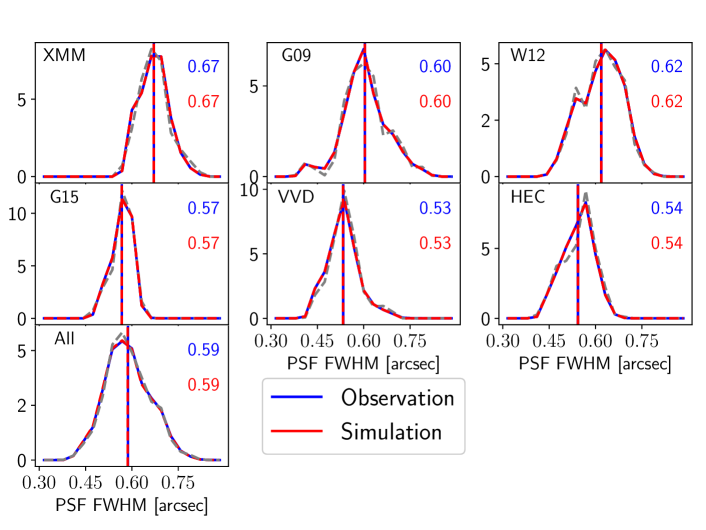
Figure 4: The first six panels show the normalized number histograms of PSF FWHM for the galaxies in the HSC observational fields. The last panel is the histogram for galaxies in all fields. The blue solid (red dashed) lines are for the HSC data (simulation). The blue (red) text and vertical lines indicate the mean averages of the HSC data (simulation). The simulations are reweighted to mitigate the difference to the data due to the finite sampling for each field. The gray lines show the histograms before the reweighting.

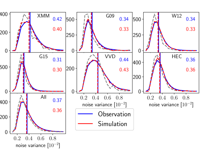
Figure 5: Same as Fig. 4, but for noise variance.

Note that the input PSF models do not include PSF model errors; that is, the PSF is assumed to be known perfectly. In addition, we assume the sky subtraction is perfect, and the residuals of the sky background are not included in the simulations. As these observational conditions are obtained from coadded images, the systematics related to the coaddition process can not be tested with the simulations.

3.2.2 Input galaxy

Mandelbaum et al. (2018b) selected galaxy training samples with CModel magnitudes less than $25.2$ from the HSC Wide-depth catalogs detected from three stacks of the HSC Deep/Ultradeep images with typical seeings of $0\farcs 5$, $0\farcs 7$, and $1\farcs 0$, respectively, in the COSMOS region (Aihara et al., 2018a). Mandelbaum et al. (2018b) determined the centroids of these galaxies on the exposures of the COSMOS HST Advanced Camera for Surveys (ACS) field (Koekemoer et al., 2007) in the F814W band. Square postage stamps centered at the galaxy centroids with width$=10\farcs 752$ ($64$ HSC pixels) were cut out from the HST exposures. The details of the training samples are described in Mandelbaum et al. (2018b). In this paper, we use the training sample selected from the stack with the best seeing ($0\farcs 5$) since it should be the deepest sample among the three thanks to its best seeing.

Note, we do not inject parametric galaxies into images as in, for example, MacCrann et al. (2020). Instead, we directly cut out postage stamps from the HST F814W images. Since we do not perform any deblending or masking on the input HST images before shearing and transforming the noise property, all of the neighboring sources are kept on the postage stamp to reproduce the effects of both recognized and un-recognized blends. We do not input star images into the simulation. Stars could appear on galaxy outskirts (not at the centers of the postage stamp) if they happens to reside in close proximity to the simulated central galaxy. We will further test the influence of stellar contamination in our shear catalog in Section 3.3.1.

GalSim (Rowe et al., 2015), which is an open-source package for galaxy image simulations, is used to simulate HSC-like images using the COSMOS HST images in our simulations. The original HST PSF is deconvolved from each input HST postage stamp and then the image is rotated with a random angle, sheared by a known input shear distortion, convolved with a collected HSC PSF model, sampled at the HSC pixel scale, and downgraded to an HSC noise level. The noises and PSFs used in the simulations are those introduced in Section 3.2.1.

Each subfield is designed to specifically include $90\degree$ rotated (intrinsically orthogonal) pairs of galaxies that can be used to nearly cancel out shape noise (Massey et al., 2007b). By keeping track of the members of each orthogonal pairs, the analysis framework provides options to apply this cancellation or not. The orthogonal pairs will also be used to derive shape measurement error, weight bias, and selection bias in the shear estimation following Mandelbaum et al. (2018b).

3.3 Weak lensing galaxy sample

3.3.1 Galaxy selection

We run $\texttt{hscPipe}~{}{\rm v}7$, the pipeline used to process the S19A internal data release along with the same configuration options, on the simulations for source detection and deblending. Subsequently, $\texttt{hscPipe}~{}{\rm v}7$ is used to perform magnitude, size and shape measurements on the deblended sources. For all of the analyses shown in this paper based on our image simulations, a basic set of flag cuts in the “Basic flag cuts” section of Table 2 are imposed. Since our simulations do not include image artifacts, only the following flags actually influence the source selection in the simulations: i$\_$detect$\_$isprimary, i$\_$sdsscentroid$\_$flag, and i$\_$extendedness$\_$value.

Following Mandelbaum et al. (2018b), we only keep the detected source nearest to the postage stamp center for each postage stamp. In addition, we require the nearest source to have a centroid that is a maximum of $5$ pixels from the postage stamp center to eliminate stamps where the detection nearest to the center was not the intended central object.

Since the input galaxy sample has an $i$-band magnitude limit of $\sim 25.2$, our simulations are not complete, especially at the very faint end. However, HSC reaches the 26’th magnitude depth thanks to its longer exposure time than HST. As a result, the input training sample is not representative to the HSC galaxies at very faint end. We also note that our simulations do not include realistic large-scale background light. However, the remaining residuals after background subtraction are likely to influence the galaxy measurements, especially on faint galaxies – and the residuals can also lead to fake detections that cannot be reproduced in our simulations.

To mitigate the difference between the simulations and the real data due to the incompleteness of the input HST galaxy training sample and the absence of realistic background light residuals, a set of cuts on galaxy properties measured with the pipeline are applied in both the HSC data and the simulations to define a high-SNR, well-resolved galaxy sample for the weak lensing science. These cuts serve to remove faint galaxies that are beyond the magnitude limit of the HST galaxy sample. In addition, such weak lensing cuts are useful to remove fake detections cased by background light residuals that is not included in our simulations. The $i$-band cuts, applied to both the observations and the simulations, are summarized in Table 2.

The cut on i$\_$extendedness$\_$value is applied to reduce stellar contamination in the weak lensing galaxy catalog. We estimate the stellar contamination fraction, the number fraction of misclassified stars in our weak lensing galaxy sample even after this cut, using as a reference the galaxy-star classification performed on HST COSMOS data by Leauthaud et al. (2007). Since the HST images have a much higher resolution and lower noise level than the HSC images, we regard the HST galaxy-star separation as the ground truth.

Fig. 6 shows the stellar contamination fractions as a function of magnitude for the catalogs selected using the weak lensing cuts in the COSMOS region. For this purpose, we utilize the Deep/Ultradeep data which consists of multiple exposures in the COSMOS region. We have constructed three different Wide-depth stacks of the HSC S19A images. These stacks correspond to the exposures with the best, median, and worst seeing, respectively, with typical seeing values of $0\farcs 5$, $0\farcs 7$, and $1\farcs 0$, respectively (Aihara et al., 2018a). Even in the worst seeing conditions, the stellar contamination fraction is below $0.2\%$ for galaxies with $i$-band magnitudes brighter than $22$, increasing to $0.5\%$ at the faintest end of the shear catalog with $i$-band magnitude close to $24.5$. Hence we conclude that the shear estimation biases from the misclassification of stars as galaxies is negligible, since the fraction of misclassified stars is less than $0.5\%$.

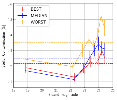
Figure 6: The stellar contamination fraction due to the incorrect classification by $\texttt{hscPipe}~{}{\rm v}7$, estimated after application of the weak lensing cuts in Table 2. We show the stellar contamination fraction as a function of $i$-band CModel magnitude for three different seeing conditions (i.e., BEST, MEDIAN, and WORST) estimated with reference to COSMOS HST star-galaxy classifications used as an estimate of ground truth. Errorbars show the Poisson uncertainties. Dashed lines show the stellar contamination fractions for all magnitude bins in the corresponding seeing samples.

We do not apply any cuts to remove the potential contamination from binary stars as in Hildebrandt et al. (2017b). Even though we do find that objects in the weak-lensing sample with extremely large ellipticity $\absolutevalue{e}>0.8$ and $i$-band determinant radius $r_{\mathrm{det}}<10^{-0.1r+1.8}$ arcsec show a characteristic stellar locus in the ($g$-$r$, $r$-$i$) color-color histogram, its number fraction is only $\sim 0.61\%$ of the weak-lensing galaxy sample, which is not likely to cause biases beyond the weak-lensing requirements. We will remove these potential binary stars from our sample in the three-year cosmological analysis.

In addition to the $i$-band cuts, we follow Mandelbaum et al. (2018a) and apply a multi-band detection cut to ensure that we have enough color information to compute photometric redshifts. The multi-band color cut requires at least two other bands (out of $grzy$-bands) to have at least a $5\sigma$ CModel detection significance (i.e., SNR$>5$). The multi-band detection cut is applied only on the HSC data but not on the image simulations since, unfortunately, we do not have multi-band image simulations. This multi-band detection cut removes a very small fraction ($<1\%$) of galaxies that pass other selection thresholds. Therefore, the multi-band cut is not likely to cause significant selection bias on the shear estimation. On the other hand, this multi-band cut helps remove junk detections and artefacts (Hildebrandt et al., 2017c).

Compared with the S16A data, the S19A data is processed with a global background subtraction scheme as summarized in Section 2.3. The under-subtraction of sky background in this scheme increases the CModel flux estimation near bright objects, which makes cuts on CModel flux inefficient at removing the galaxies beyond the HST magnitude limit and the fake detections caused by background light residuals in the observations. We find a mismatch in the SNR-$R_{2}$ $2$D histograms between the S19A HSC data and the simulations at the faint end when simply using the first-year $i$-band cuts summarized in Table 4 of Mandelbaum et al. (2018a). There are more extended faint detections that are very likely to be fake detections in the HSC data than in the simulations. Therefore, we apply an additional cut on $i$-band $1\arcsec$-diameter-aperture magnitudes (mag_A) at $25.5$ to remove the fake detections that cannot be reproduced in the simulations. The additional aperture magnitude cut removes $3.9\%$ of the galaxies that pass other selection cuts. The selection bias due to the cuts is quantified in Section 3.7.

Table 2: Weak lensing cuts: The $i$-band selection criteria that are applied to both the simulations and the HSC data. We note that the “i$\_$pixelflags$\_$clipped $==$ False” (“i$\_$pixelflags$\_$edge $==$ False”) flag, which identifies detections close to the artifacts (edges) resulting in unreliable PSFs, was not properly set in the first-year shear catalog. As described in Section 4.9 of Aihara et al. (2019), the flags are correctly set for the current data.

Cut	Meaning
Basic flag cuts
i$\_$detect$\_$isprimary $==$ True	Identify unique detections only
i$\_$deblend$\_$skipped $==$ False	Deblender skipped this group of objects
i$\_$sdsscentroid$\_$flag $==$ False	Centroid measurement failed
i$\_$pixelflags$\_$interpolatedcenter $==$ False	A pixel flagged as interpolated is close to object center
i$\_$pixelflags$\_$saturatedcenter $==$ False	A pixel flagged as saturated is close to object center
i$\_$pixelflags$\_$crcenter$==$ False	A pixel flagged as a cosmic ray hit is close to object center
i$\_$pixelflags$\_$bad$==$ False	A pixel flagged as otherwise bad is close to object center
i$\_$pixelflags$\_$suspectcenter $==$ False	A pixel flagged as near saturation is close to object center
i$\_$pixelflags$\_$clipped $==$ False	Source footprint includes clipped pixels
i$\_$pixelflags$\_$edge $==$ False	Object too close to image boundary for reliable measurements
i$\_$hsmshaperegauss$\_$flag $==$ False	Error code returned by shape measurement code
i$\_$hsmshaperegauss$\_$sigma $!=$ NaN	Shape measurement uncertainty should not be NaN
i$\_$extendedness$\_$value $!=0$	Extended object
Galaxy property cuts
i$\_$cmodel$\_$flux/i$\_$cmodel$\_$fluxerr $\geq 10$	Galaxy has high enough $S/N$ in $i$-band
i$\_$hsmshaperegauss$\_$resolution $\geq 0.3$	Galaxy is sufficiently resolved
(i$\_$hsmshaperegauss$\_$e1${}^{2}+$i$\_$hsmshaperegauss$\_$e2${}^{2})^{1/2}<2$	Cut on the amplitude of galaxy ellipticity
$0\leq$i$\_$hsmshaperegauss$\_$sigma $\leq 0.4$	Estimated shape measurement error is reasonable
i$\_$cmodel$\_$mag $-$ a$\_$i $\leq 24.5$	CModel Magnitude cut
i$\_$apertureflux$\_$10$\_$mag $\leq 25.5$	Aperture ($1\arcsec$ diameter) magnitude cut
i$\_$blendedness$\_$abs $<10^{-0.38}$	Avoid spurious detections and those contaminated by blends

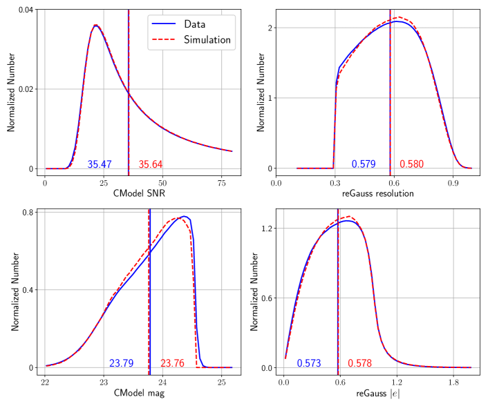
Figure 7: The normalized number histograms of $i$-band properties including CModel SNR (upper left), reGauss resolution (upper right), CModel magnitude (lower left), and reGauss ellipticity magnitude (lower right), for galaxies in all fields combined. The blue solid (red dashed) lines are for the HSC data (simulation). The blue (red) text and vertical lines indicate the mean averages of the HSC data (simulation).

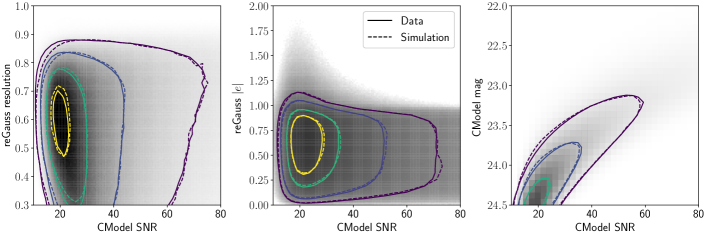
Figure 8: The color maps are the $2$D histograms for the HSC data. The panels from left to right show the (SNR, $R_{2}$), (SNR, $|e|$) and (SNR, CModel magnitude) histograms, respectively. The solid (dashed) lines show the contours for the HSC data (simulation). The contours in panels from left to right are defined at (0.90, 0.60, 0.30, 0.12), (0.76, 0.54, 0.26, 0.14), and (0.68, 0.34, 0.14) of the maximums of the corresponding histograms.

To study the influence of the selection function of $\texttt{hscPipe}~{}{\rm v7}$ source detection on our galaxy sample, in cases where no object is detected within $5$ pixels from the center of a simulated postage stamp, we artificially force one detection with its peak at the center of the stamp. Flux, size and shape measurements are conducted on the artificially forced detections. We find that the number of these forced detections that enter the weak lensing sample after the weak lensing cuts are applied is far less than $0.1$% of the total galaxy number in the weak lensing sample, which indicates that the selection function of the source detector has a negligible influence on the weak lensing sample; therefore, the selection bias from the source detector is negligible. This is aligned with our expectations, since the $5\sigma$ detection limit for point sources is $26.2$ mag in $i$-band, and our weak lensing galaxy sample is selected with an $i$-band magnitude cut at $24.5$, far brighter than the detection limit. We note that one limitation of our simulations is that several defects from real data (e.g., sky background residuals, optical ghosts, very bright stars, etc.) that can affect the object detection are not included.

3.3.2 Galaxy properties

The $1$D normalized number histograms for $i$-band galaxy properties (i.e., CModel SNR, reGauss resolution, CModel magnitude, reGauss ellipticity magnitude defined as $|e|=\sqrt{e_{1}^{2}+e_{2}^{2}}$), in the HSC observations and the simulations are shown in Fig. 7. When plotting the histograms, we adopt the same upper limit on the $i$-band CModel SNR (SNR$<80$) as Mandelbaum et al. (2018b) to compare our results with those shown in the HSC first-year image simulation paper. We do not find significant differences in the shapes of the number histograms between the HSC data and the simulations. The relative difference of the mean values averaged across all of the fields for these properties between the data and the simulations are $0.5\%$ (CModel SNR), $0.2\%$ (reGauss resolution) $0.1\%$ (CModel mag) and $0.8\%$ ($|e|$), all of which are less than $1\%$. Finally, we show the $2$D joint histograms of these galaxy properties in Fig. 8.

Compared to the first-year HSC-like image simulations (see Mandelbaum et al., 2018b, Fig. 8), the three-year HSC-like simulations have a better match to the HSC data in the SNR histogram. The average SNR over all fields was relatively less than the observed SNR by $\sim 5\%$ in Mandelbaum et al. (2018b), while the discrepancy decreases to $\sim 0.5\%$ for the three-year HSC-like image simulations presented in this paper. The match in SNR distribution improves because we rescale the sampled noise variance for a consistent match between the measured noise variances from the HSC data and those from the simulations as discussed in Section 3.2.1. Furthermore, the matches between the $2$D histograms are visually better than those of the first-year HSC simulations shown in Fig. 9 of Mandelbaum et al. (2018b), primarily due to the improvement in the match between the SNR histograms.

In addition, compared to the state-of-art image simulations in other weak lensing surveys, e.g., Fig. 3 in MacCrann et al. (2020) from the DES survey and Fig. 9 in Kannawadi et al. (2019) from the KiDS survey, our simulations generally have better matches to the observations in the histograms of galaxy brightness, size and shape.

3.4 Optimal weighting

In this section, we estimate and model the statistical uncertainties from photon noise (shape measurement error) and shape noise (intrinsic shape dispersion) as functions of galaxy properties, and determine the optimal weight for the shear estimation.

We first use the simulations to estimate the $1\sigma$ per-component shape uncertainty due to photon noise ($\sigma_{e}$) and model it as a function of galaxy properties (i.e., SNR and $R_{2}$) following the formalism given in Appendix A of Mandelbaum et al. (2018b). In the estimation, we use the orthogonal galaxy pairs to nearly cancel out shape noise and measure the statistical error due to photon noise.

We define a sliding window in the (SNR, $R_{2}$) plane with an equal-number binning scheme and estimate $\sigma_{e}$ in each bin. The results of this process are shown in the left panel of Fig. 9. In order to estimate $\sigma_{e}$ for each galaxy in the catalog, we fit a power-law $\sigma_{e}({\rm SNR},R_{2})$ to the estimated $\sigma_{e}$, such that

$$\sigma_{e}=0.268\left(\frac{{\rm SNR}}{20}\right)^{-0.942}\left(\frac{R_{2}}{0.5}\right)^{-0.954},$$ (11)

and linearly interpolate the ratio of the estimated values to the fitted power-law based on the $\log_{10}({\rm SNR})$ and $R_{2}$ values. For SNR and $R_{2}$ outside the bounds of the sliding window, the nearest point within the sliding window is used for the interpolation of this ratio. As shown, the shape measurement error from photon noise is a decreasing function in the SNR direction and the $R_{2}$ direction since noise has less influence on bright, large galaxies.

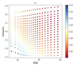
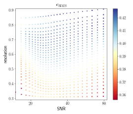
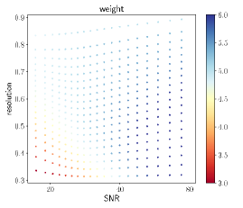
Figure 9: The left panel shows the $1\sigma$ per-component shape measurement uncertainty ($\sigma_{e}$) estimated with the simulations in different (SNR, $R_{2}$) bins. The middle panel is for the estimated per-component intrinsic shape dispersion ($e_{\rm{RMS}}$) following Eq. (12). The right panel is for the estimated optimal weight.

Using galaxies in the real HSC shear catalog, we estimate the per-component intrinsic shape dispersion ($e_{\rm{RMS}}$) by subtracting off (in quadrature) the shape measurement error from the shape dispersion such that

$$e_{{\rm RMS}}=\sqrt{\frac{\sum_{i}\left(e_{1;i}^{2}+e_{2;i}^{2}-2\sigma_{e}^{2}({\rm SNR}_{i},R_{2;i})\right)}{2N_{\text{gal}}}},$$ (12)

where $i$ is the galaxy index and $N_{\text{gal}}$ refers to the number of galaxies in the galaxy ensemble. This estimate is computed in each sliding window, and the estimated intrinsic shape dispersion as a function of the position in the (SNR, $R_{2}$) plane is shown in the middle panel of Fig. 9. As shown, the intrinsic shape is a relatively flat function on the $2$D plane, with a value around 0.4 for most of parameter space. The corresponding optimal weight defined in Eq. (4) is shown in the right panel of Fig. 9. The shape dispersion is relatively flat with a value around $0.4$; therefore, we linearly interpolate the function in the $2$D plane to model $e_{{\rm RMS}}$ on the individual galaxy level. The optimal weight is determined with $\sigma_{e}$ and $e_{{\rm RMS}}$ following Eq. (4). The responsivity is determined following Eq. (5).

3.5 Calibration

In this section, we estimate, model, and remove the shear calibration bias, except for selection bias, which will be quantified and removed in Section 3.7. The formalism we applied here generally follows that introduced in Section 4.5 of Mandelbaum et al. (2018b) but with several subtle differences that we explicitly flag. We refer readers to Section 4.2 and 4.4 for the HSC three-year weak-lensing science requirements on the residual multiplicative bias ($\absolutevalue{\delta m}<9.3\times 10^{-3}$) and the fractional additive bias ($\absolutevalue{\delta a}<9.7\times 10^{-3}$), respectively.

3.5.1 Baseline calibration

In order to determine the baseline shear calibration bias in the absence of selection bias, we keep both galaxies in each $90\degree$ rotated pair by imposing the weak lensing cuts on only one randomly chosen galaxy in the pair. In addition, we force both galaxies in each pair to use the same shape weight of the randomly chosen galaxy, to avoid weight bias due to the correlation of shape weight with shear. By doing so, we ensure that both our selection and weighting processes do not correlate with the input shear, since we wish to separately quantify and remove those effects.

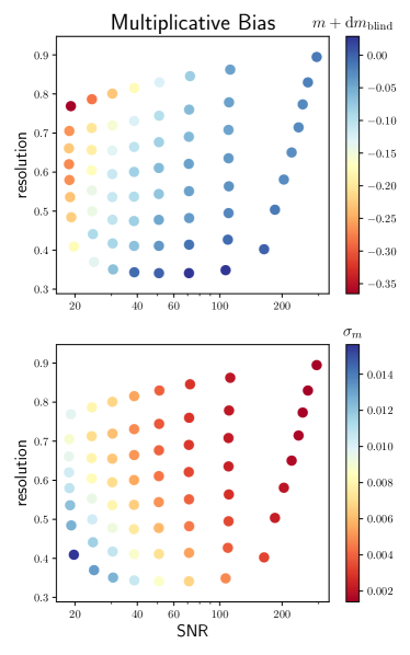
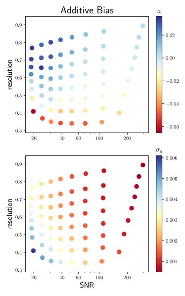
Figure 10: The left panels show the multiplicative bias (upper left) and its standard deviation (lower left) estimated in the (SNR,$R_{2}$) plane using the image simulations. The right panels are for the fractional additive bias. Note that the multiplicative bias is blinded by adding a shift $dm_{\rm blind}$.

In the upper left panel of Fig. 10, we show the baseline multiplicative bias as a function of position in the (SNR, $R_{2}$) plane with an equal-number binning scheme for the overall simulation. When making the figure, an unspecified constant value is added to the multiplicative bias to blind our shear analysis. For reference, the lower left panel shows the standard deviation of the multiplicative bias estimation in the upper left panel. Similarly to what was done to model the shape measurement error in Section 3.4, we fit $m({\rm SNR},R_{2})$ to a power-law in both parameters plus a constant offset. The best-fit power-law is shown as follows:

$$m({\rm SNR},R_{2})+{\rm const.}\propto\left(\frac{R_{2}}{0.5}\right)^{1.66}\left(\frac{{\rm SNR}}{20}\right)^{-1.24}\,.$$ (13)

We then interpolate a correction to the power-law based on the ratio between the multiplicative bias estimation and the power-law, and the interpolation scheme is the same as that for the shape measurement error due to photon noise.

In the upper right panel of Fig. 10, we show the baseline fractional additive bias as a function of position in the (SNR, $R_{2}$) plane with an equal-number binning scheme for the overall simulation. For reference, the lower right panel shows the standard deviation of the additive bias estimation in the upper left panel. Similarly to the modelling of the baseline multiplicative bias, we fit the estimated baseline fractional additive bias to the model proposed in Mandelbaum et al. (2018b). The best-fit model is shown as follows:

$$a({\rm SNR},R_{2})\propto(R_{2}-0.61)\left(\frac{{\rm SNR}}{20}\right)^{-0.94}\,.$$ (14)

Subsequently, we interpolate a correction to the model based on the difference between the fractional additive bias estimation and the model.

3.5.2 Weight bias

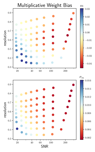
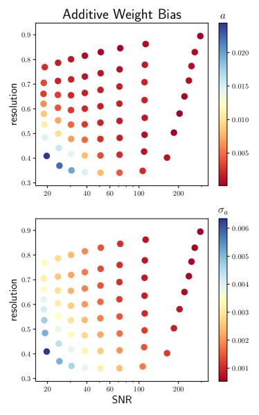
Figure 11: The left panels show the multiplicative weight bias (upper left) and the standard deviation (lower left) of the multiplicative bias estimated in the (SNR,$R_{2}$) plane using the simulation. The right panels are for the fractional additive weight bias.

Weight bias refers to the bias in estimated shear due to a correlation between the adopted shape weight and the true lensing shear. It can also be regarded as the bias from a shear-dependent smooth selection, since weighting is effectively a smooth selection (Mandelbaum et al., 2018b). Weight bias can be corrected analytically if the response of the weight to the shear distortion is known (e.g., Li et al., 2018). On the other hand, weight bias can also be estimated using image simulations containing $90\degree$ rotated pairs (Mandelbaum et al., 2018b).

Here we follow the scheme of Mandelbaum et al. (2018b) to estimate weight bias using image simulations by comparing the shear bias estimation with and without enforcing the same shape weight for each galaxy in an orthogonal galaxy pair. In Fig. 11, we show the multiplicative weight bias (left panel) and the fractional additive weight bias (right panel). The binning scheme here is the same as used in Section 3.5.1. We find a statistically significant multiplicative weight bias that depends on galaxy properties. As shown, this bias is negative and reaches a maximum amplitude of $-0.045$ at high SNR and $R_{2}$, while it is positive and reaches a maximum amplitude of $0.03$ at low SNR and $R_{2}$. We also find a small additive weight bias with $\lesssim 5\sigma$ significance. The additive weight bias reaches its maximum of $0.025$ at low SNR and $R_{2}$, and it decreases as SNR and $R_{2}$ increase.

Considering that the weight biases are dependent on the location in the $2$D plane, we use the same process as in Section 3.5.1 to model and interpolate the weight biases as functions of position in the $2$D plane.

3.5.3 Redshift dependence

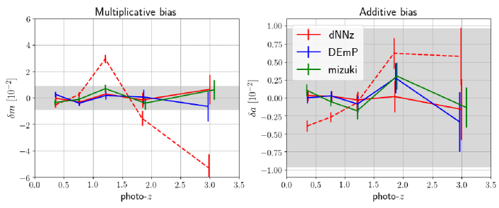
Figure 12: The left (right) panel shows the redshift-dependent multiplicative (fractional additive) bias. The red lines are for dNNz photo-$z$, the blue lines are for DEmP photo-$z$, and the green lines are for mizuki photo-$z$. The dashed lines are the results before removing the redshift-dependent bias, whereas the solid lines are the results after modelling and calibrating the redshift-dependent bias with dNNz photo-$z$. The gray regions indicate the requirements on calibration residuals that will be defined in Section 4.

Since weak lensing analyses often divide the galaxy sample into different photometric redshift (photo-$z$) bins (e.g., Hikage et al., 2019a; Hamana et al., 2020), or use photometric redshift-dependent weights (e.g., Murata et al., 2019; Miyatake et al., 2019), quantifying and correcting the redshift-dependent shear calibration biases are crucially important. We note that some redshift-dependent biases are already partially accounted for by the calibrations in Sections 3.5.1 and 3.5.2, which model the calibration biases as functions of $R_{2}$ and SNR. In this section, we look into the remaining redshift dependence of the shear estimation biases after those effects are already accounted for.

Currently, we only have realistic simulations for $i$-band images since our input galaxy sample are from the single-band F814W HST exposures. Therefore, photometric redshifts cannot be directly derived from our simulated images. We will follow Li et al. (2020), and use the photo-$z$ estimates of the input galaxies as a proxy of the measured redshift in the simulations to study the redshift-dependent shear estimation biases.

In particular, we match the input COSMOS galaxies to the HSC S19A photo-$z$ catalog in the Wide layer according to the angular position of the input galaxies, and assign each galaxy in the simulations the estimated redshift of the matched galaxy in the HSC photo-$z$ catalog.

For cross validation, we use three different HSC photo-$z$ estimates: the Deep Neural Net Photometric Redshift (dNNz; Nishizawa et al., in prep.), Direct Empirical Photometric code (DEmP; Hsieh & Yee, 2014), and Mizuki photometric redshift (mizuki; Tanaka, 2015), which are based on neural network, empirical polynomial fitting, and Bayesian template fitting, respectively. To be specific, we estimate and remove calibration bias as a function of the dNNz photo-$z$. Then we use the DEmP photo-$z$ and the mizuki photo-$z$ for cross-validation tests. The details of the DEmP and the mizuki photo-$z$ catalogs are summarized in Nishizawa et al. (2020), and the dNNz photo-$z$ catalog is described in Nishizawa et al. (in prep.).

We divide the simulations into dNNz photo-$z$ bins of equal-numbers of galaxies with selection bias cancellation by enforcing that orthogonal galaxy pairs are in the same bin. The multiplicative and additive bias are estimated for each bin. Then we compare the estimated biases with the predicted biases using the calibration model derived in Sections 3.5.1 and 3.5.2. Here, we force the shape noise cancellation by using orthogonal galaxy pairs to cancel out selection bias due to galaxy cuts, while we do not force the galaxy pairs to have the same shape weight to cancel weight bias, because weight bias has already been estimated and included in the calibration parameters (see Section 3.5.2).

The dashed red lines in Fig. 12 show the residuals of multiplicative bias (left panel) and additive bias (right panel) as a function of dNNz redshift. We model the redshift-dependent biases by linearly interpolating the bias residuals across the redshift bins.

We note that the first-year HSC shear calibration paper find a redshift dependence of the per-component intrinsic shape dispersion ($e_{\rm{RMS}}$) using a training sample of parametric galaxies fitted to the COSMOS HST galaxies with redshift ranging from $0$ to $1.5$. Mandelbaum et al. (2018b) estimated the multiplicative bias caused by such redshift dependence, and reported a multiplicative biases of $-1\%$ and $3\%$ for galaxies in the photo-$z$ range $[0,1]$ and $[1,1.5]$, respectively. Our estimation of redshift-dependent multiplicative bias has the same trend as that in Mandelbaum et al. (2018b) in the redshift range $[0,1.5]$. In contrast, our estimation covers the redshift range $[0,4]$ and includes all sources of redshift-dependent shear measurement bias. The redshift-dependent additive bias is shown in the right panel of Fig. 12; even prior to correction, it is within the three-year systematic error requirements that will be defined in Section 4.

3.5.4 Combined estimates of calibration bias

The final multiplicative bias and additive bias estimates for each galaxy in the catalog are the sum of the baseline bias modeled in Section 3.5.1, the weight bias modeled in Section 3.5.2, and the residual redshift-dependent bias modeled in Section 3.5.3. The outputs of the calibration are summarized in Table 3.

Table 3: The outputs from the analyses based on the image simulations. The first three outputs are derived to optimize the shear estimation as described in Section 3.4. The last three outputs are derived to calibrate the shear estimation as described in Section 3.5.1, Section  3.5.2, and Section 3.5.3.

Output properties	Meaning
Optimization
i$\_$hsmshaperegauss$\_$derived$\_$sigma$\_$e	Measurement error from photon noise
i$\_$hsmshaperegauss$\_$derived$\_$rms$\_$e	Shape noise dispersion
i$\_$hsmshaperegauss$\_$derived$\_$weight	Weak lensing shape weight
Calibration
i$\_$hsmshaperegauss$\_$derived$\_$shear$\_$bias$\_$m	Multiplicative bias
i$\_$hsmshaperegauss$\_$derived$\_$shear$\_$bias$\_$c1	The first component of additive bias
i$\_$hsmshaperegauss$\_$derived$\_$shear$\_$bias$\_$c2	The second component of additive bias

3.6 Ensemble calibration uncertainties

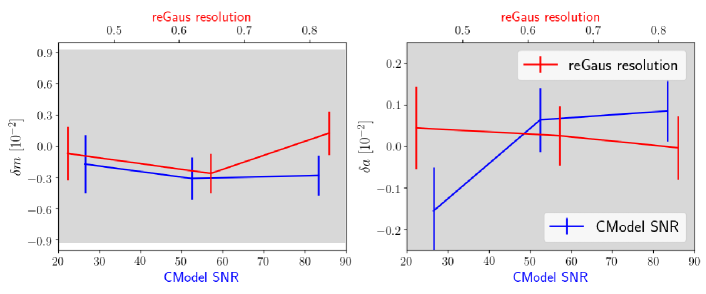
Figure 13: The calibration residuals for subsamples binned by two modeled galaxy properties ,i.e., $R_{2}$ (red) and SNR (blue). The left (right) panel shows the multiplicative (fractional additive) bias. The gray regions indicate the requirements on calibration residuals that will be defined in Section 4.

This section serves to demonstrate the validity and robustness of the calibration of the shear biases (i.e., multiplicative bias and additive bias) derived in Section 3.5, and assign a systematic uncertainty to the calibration at the ensemble level. We focus on the systematic calibration residuals for multiplicative bias ($\delta m$) and fractional additive bias ($\delta a$), which are the remaining bias after the shear calibration of Section 3.5. The selection bias is not taken into account here, and we force the shape noise cancellation by using orthogonal galaxy pairs to cancel out selection bias due to galaxy cuts as in Section 3.5.

First, we divide the simulations into several subsamples following an equal-number binning scheme by the galaxy properties including those used for modeling shear biases (i.e., CModel SNR, reGauss resolution, and dNNz photo-$z$) and those that are marginalized, that is, not explicitly taken into account in the bias modelling (i.e., CModel magnitude, seeing, DEmP and mizuki photo-$z$). Shear is subsequently estimated for each subsample in each subfield using the calibrated shear estimator. Finally, we determine the bias residuals for each property-binned subsample using Eq. (6).

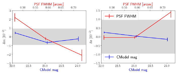
Figure 14: The calibration residuals for subsamples binned by two marginalized galaxy properties, i.e., seeing size (red) and CModel magnitude (blue). The left (right) panel shows the multiplicative (fractional additive) bias. The gray regions indicate the requirements on calibration residuals defined in Section 4.

The red solid lines in Fig. 12 show the bias residuals with dNNz photo-$z$ binning. Fig. 13 shows the calibration bias residuals when binning the simulations with SNR or $R_{2}$. The results demonstrate that the amplitude of the multiplicative bias residual ($\delta m$) is less than $0.5\%$, the fractional additive bias residual ($\delta a$) is less than $0.5\%$, both of which are within the systematic error requirements that will be defined in Section 4. These bias residuals are expected to be consistent with zero since these galaxy properties were used to model the calibration bias calibration.

Finally we test the dependence of the bias residuals on the marginalized properties. We demonstrate the bias residuals when binning galaxies by DEmP and mizuki photo-$z$ in Fig. 12. Fig. 14 shows the bias residuals when binning the simulations with CModel magnitude and seeing size. We do not find calibration bias residuals beyond the requirement limits for the cases of DEmP photo-$z$, mizuki photo-$z$, and CModel magnitude.

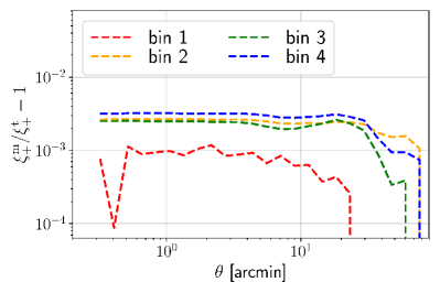
Figure 15: The relative bias on the shear-shear correlation function as a function of separation angle caused by the seeing-dependent calibration bias residual. Lines with different colors refer to the shear-shear auto-correlations in four different redshift bins.

However, when binning by seeing size, the residuals of the multiplicative bias exceed our requirements for the best and worst seeing bins, and the residuals of the fractional additive bias slightly exceed the requirements for the worst seeing bin, which is consistent with Mandelbaum et al. (2018b). The binning by seeing size corresponds to an extreme case of splitting up the survey based on regions with specific properties. Our finding implies that weak lensing analyses with strict area cuts should evaluate the seeing distribution after the cuts, and then evaluate whether additional shear calibration biases are required to be removed for such an area. For a weak lensing analysis that neither weights galaxies by the seeing size nor divides galaxies into seeing bins, the calibration bias residuals shown by the red lines in Figure 14 will not bias the analysis, since the calibration bias residuals averaging over seeing sizes are within the requirement limits. It suggests that this result is not relevant to the cosmic shear analysis and the galaxy-galaxy lensing analysis using lens samples covering the entire HSC survey area (e.g., CMASS galaxy sample; Reid et al., 2016a).

However, we test the impact of this seeing-dependent calibration bias more rigorously with a realization of the three-year HSC mock catalog (Shirasaki et al., in prep.) constructed using the full-sky lensing simulation of Takahashi et al. (2017). The mock catalog uses the angular coordinates, seeing sizes, galaxy fluxes, photo-$z$ estimation etc. of the HSC shape catalog, and it samples the true redshift for each galaxy using its dNNz photo-$z$ posterior distribution; therefore, the mock has the same spatial distribution of the seeing as the data. Lensing shear from the full-sky lensing simulation is assigned to each galaxy according to its position, and shape noise is not included in this test. We fit the calibration residual shown by the red line in the left panel of Figure 14 as a function of seeing FWHM with a linear model and use the derived model to assign a multiplicative bias for each galaxy in the mock according to its seeing size. Note that when ignoring the seeing dependence, the multiplicative bias should give zero spurious shear correlations. We subsequently divide galaxies in the mock into four redshift tomographic bins from $z=0.3$ to $z=1.5$ with equal separation following Hamana et al. (2020) and compute the shear-shear autocorrelation function in each redshift bin. In Figure 15, we show the relative difference between the results from the mock with the seeing-dependent multiplicative bias residual (denoted as $\xi^{\rm m}_{+}$) and the results from the same mock but without multiplicative bias (denoted as $\xi^{\rm t}_{+}$). The results show that the relative difference is less than 0.4%, and the resulting bias on $S_{8}=\sigma_{8}(\Omega_{\rm m0}/0.3)^{0.5}$ should be less than 0.2%. The method of accounting for calibration uncertainties for galaxies in each tomographic bin in the cosmic shear analysis will be discussed in detail in the cosmic shear paper.

3.7 Selection bias

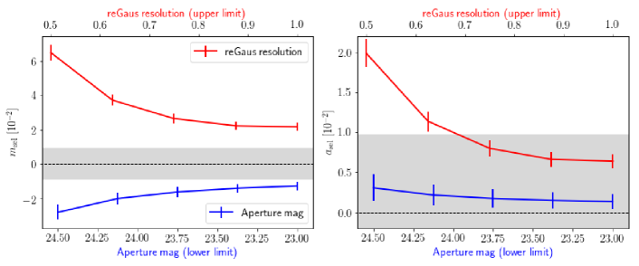
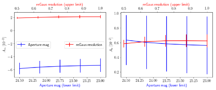
Figure 16: The upper left (upper right) panel shows the multiplicative (fractional additive) bias due to cuts on resolution $R_{2}$ (red) and aperture magnitude mag_A (blue). The gray regions indicate the requirements on calibration residuals defined in Section 4, and the horizontal dashed lines are $y=0$. The lower left (lower right) panel shows the multiplicative (fractional additive) bias ratio of the cuts on resolution $R_{2}$ and aperture magnitude mag_A. For resolution, we fix the lower limit and change the upper limit. For aperture magnitude, we fix the upper limit and change the lower limit. For each selection cut, errorbars are correlated between the points since at least a fraction of the same simulated galaxies are used for the calculations.

Given that the amplitudes of the lensing shear and the PSF anisotropy are small, the anisotropic selection has little influence on the galaxies that are far away from the selection edge. The selection bias should be proportional to the marginal density at the edge (see Li et al., 2021, for analytical correction of selection bias). Here we follow Mandelbaum et al. (2018b) to empirically estimate the selection bias by comparing the shear estimation of the overall sample with/without forcing the inclusion of $90\degree$ rotated pairs.

We focus on the correction for the selection bias due to cuts on resolution and aperture magnitude, as we find that the selection biases for other cuts on $i$-band galaxy properties (e.g., CModel SNR, CModel Magnitude) are consistent with zero, and the selection bias for the multi-band detection cut is negligible since the cut removes less than one percent of the galaxies from the parent sample. The upper panels of Fig. 16 show the estimated selection biases for the resolution cut ($R_{2}>0.3$) and the aperture magnitude cut (mag${}_{A}<25.5$) listed in Table 2, while changing the upper (lower) limit of resolution (aperture magnitude) to change the galaxy ensemble. We find that the multiplicative bias for the resolution (magnitude) cut is constantly positive (negative), and the fractional additive bias for the resolution cut is constantly positive. The fractional additive bias for the aperture magnitude cut is consistent with zero within $2\sigma$ and is within the three-year HSC science requirement. As we expect, the amplitudes of the biases decrease when the sizes of the corresponding galaxy ensembles increase since the fractions of the galaxies that are close enough to the selection edges and are influenced by the anisotropic selections decrease.

In order to empirically estimate and remove the selection bias for any galaxy sample due to the two aforementioned cuts, we adopt the method proposed by Mandelbaum et al. (2018b). The premise of the method is that, for a galaxy sample, the ratio between the selection biases, from a cut on galaxy observable ($X$), versus the marginal galaxy number density at the edge of the cut ($P(X)\mid_{{\rm edge}}$) is approximately constant. The selection bias ratios are defined as

$$\begin{split}A_{m}(X)=\frac{m^{\mathrm{sel}}\left(X\right)}{P\left(X\right)\mid_{{\rm edge}}},\\ A_{a}(X)=\frac{a^{\mathrm{sel}}\left(X\right)}{P\left(X\right)\mid_{{\rm edge}}}\,.\end{split}$$ (15)

The lower panels of Fig. 16 show the selection bias ratios for $R_{2}$ and mag_A. Here we fix the lower limit of resolution at $R_{2}=0.3$ and the upper limit of aperture magnitude at mag${}_{A}=25.5$, respectively. Then we adjust the upper limit of $R_{2}$ and the lower limit of mag_A to change the galaxy sample.

As demonstrated by the lower panels of Fig. 16, the selection bias ratios vary slowly with the change of the galaxy sample; therefore, we take the selection bias ratios as constants. The selection bias ratios are used to estimate selection biases for any galaxy sample by multiplying them by the marginal galaxy number densities at the edges of the corresponding selection cuts. The resulting multiplicative and fractional additive selection biases for $R_{2}$ and mag_A are shown as follows:

$$\begin{split}m^{\mathrm{sel}}&=-0.05854P\left(\text{mag}_{A}=25.5\right)+0.01919P\left(R_{2}=0.3\right),\\ a^{\mathrm{sel}}&=0.00635P\left(\text{mag}_{A}=25.5\right)+0.00627P\left(R_{2}=0.3\right),\end{split}$$

respectively. In cosmological analyses, this equation should be used to estimate the selection biases for specific galaxy ensembles according to the marginal galaxy number densities. The selection bias should be removed from the shear estimation if it is beyond the requirement limits.

3.8 Redshift-dependent blending

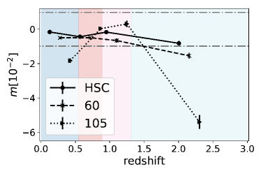
Figure 17: The excess multiplicative bias in our fiducial calibration due to redshift-dependent blending in four redshift bins as indicated by colored regions. The solid, dashed and dotted lines are for simulations with an HSC PSF with FWHM=$0\farcs 58$, Moffat PSF with FWHM$=0\farcs 6$, and Moffat PSF with FWHM$=1\farcs 05$, respectively. The errorbars are estimated using a jacknife for different noise realizations. The horizontal dash-dotted lines show the three-year HSC requirement.

The DES Y3 analysis in MacCrann et al. (2020) used parametric galaxy models with known redshifts as their image simulation training sample. They randomly populated these parametric galaxies with a detection density matched to the DES observations to simulate multi-band DES images that were used to test and calibrate METACALIBRATION (Sheldon & Huff, 2017). They tested for the circumstance that galaxies at different redshifts were distorted by different shear signals and compared the results with those from the conventional constant-shear simulations. According to Fig. 8 of MacCrann et al. (2020), the amplitude of the additional bias due to the redshift-dependent shear is below $1\%$ for redshift $z<1$, while it reaches $\sim 3$% for redshifts $1<z<3$ for the DES observational conditions.

We note that it is impossible to directly apply different shear distortions to blended galaxies separately in our fiducial simulations since they are constructed using postage stamps directly cut out from the COSMOS HST images. Therefore, galaxies in one HST postage stamp can only be distorted by a single constant shear as a whole, and any bias due to redshift-dependent blending is not included in our fiducial calibration. Here we investigate the multiplicative bias that is not captured by our fiducial calibration due to the difference between the constant-shear setup and a redshift-dependent-shear setup.

We make additional image simulations using parametric galaxy models fitted to the galaxies in the HST F814W shape catalog (Leauthaud et al., 2007). We randomly populate these parametric galaxies into a region with an area of 141 arcmin${}^{2}\,$. The density of the input galaxies is set to $\sim 88$ arcmin^-2, which is the same as MacCrann et al. (2020). The redshifts of the galaxies are set by matching the HST F814W shape catalog to the COSMOS photo-$z$ catalog (Ilbert et al., 2009) using their coordinates. The galaxies are distorted with different shears and convolved with three different PSFs (an HSC PSF with FWHM$=0\farcs 58$ and Moffat PSFs with input FWHM$=0\farcs 6$ and FWHM$=1\farcs 05$). Different realizations of pixel noise with variance set to the average of the HSC noise variance are added to the image. We confirm that, after the weak-lensing cuts, the difference between the galaxy number in the simulation (with the HSC PSF) and that of the real HSC data is less than 4%. In addition, the galaxy number histograms over galaxy properties (e.g. CModel SNR, reGauss resolution and CModel magnitude) visually match those of the real HSC data.

We first determine the calibration bias using a constant-shear setup where all of the galaxies in one image are distorted with the same shear. We simulate two images with shear distortions $\gamma_{1}=+0.02$ and $\gamma_{1}=-0.02$, with the same noise on these two images to reduce the impacts of shape and pixel noise (Pujol et al., 2019). We repeat the simulations with different noise realizations. For each image, we detect, deblend and measure the properties of the sources using the HSC pipeline. The weak-lensing cut introduced in Section 3.3.1 is then applied to the detected sources. We match the galaxies selected by the weak-lensing cut to the input galaxy catalog using their coordinates and assign each selected galaxy with the redshift of the closest match in the input galaxy catalog. We measure the difference between the average shears (over noise realization) measured from the simulations with $\gamma_{1}=+0.02$ and $\gamma_{1}=-0.02$, and divide it by the difference in the input shear distortion ($\Delta\gamma_{1}=0.04$) to determine the calibration bias. By dividing the selected galaxy into four redshift bins as indicated by the four colored regions in Figure 17, we estimate the multiplicative bias in each redshift bin.

Then we apply the multiplicative bias estimated from the constant-shear simulation to the redshift-dependent-shear simulation following MacCrann et al. (2020). For the redshift-dependent-shear setup, we select one bin from the four redshift bins and only distort the input galaxies in the selected redshift bin while leaving the galaxies in the other three redshift bins undistorted instead of distorting all galaxies with the same shear. We perform source detection, deblending and measurement using the HSC pipeline on the simulated images to obtain a galaxy shape catalog. After that, we apply the weak-lensing cut and estimate the average shear from galaxies in the selected redshift bin. In order to estimate the additional multiplicative bias due to the difference between redshift-dependent-shear setup and constant-shear setup, we use the multiplicative bias obtained from the constant-shear simulation for the selected redshift bin to calibrate the average shear measured from the redshift-dependent-shear simulation with different noise realizations and shear distortions (i.e. $\gamma_{1}=+0.02$ and $\gamma_{1}=-0.02$). We carry out this process in four redshift bins to estimate the excess multiplicative bias in each redshift bin.

Figure 17 shows the additional multiplicative bias due to redshift-dependent shear in each redshift bin for the three different seeing setups. It shows that for observations with a larger seeing size, the amplitude of the excess multiplicative bias due to redshift-dependent blending is larger. Furthermore, we find that, for the HSC PSF with FWHM close to the HSC average, the multiplicative bias due to the redshift-dependent blending that is not captured by our fiducial calibration marginally meets the three-year HSC requirement. The excess multiplicative bias will be marginalised over during the cosmological analyses.

3.9 Basic characterization of the catalog

The catalog, after applying the weak lensing cuts, covers an area of $433.48~{}{\rm deg}^{2}$, split into six fields with an overall mean $i$-band seeing of $0.59\arcsec$. The shear catalog contains $35,805,482$ galaxies, a number that is $2.95$ times that of the first-year catalog, primarily due to the increased area. The raw galaxy source number density for our catalog is $22.9~{}{\rm arcmin}^{-2}$, which is comparable with the number density of the first-year shear catalog. The effective galaxy number density, defined in Chang et al. (2013) as

$$n_{{\rm eff}}=\sum_{i}\frac{e_{{\rm RMS};i}^{2}}{\sigma_{e;i}^{2}+e_{{\rm RMS};i}^{2}},$$ (16)

is $19.9~{}{\rm arcmin}^{-2}$. The effective galaxy number density map for each field is shown in Fig. 18. In Fig. 19, we show the trend of the average effective number density as a function of the PSF FWHM for each field. As shown, the effective number density slowly decreases as the PSF FWHM increases. Since the resolution of a galaxy decreases when the PSF FWHM increases, the resolution cut ($R_{2}>0.3$) tends to remove more galaxies in the regions with larger seeing sizes.

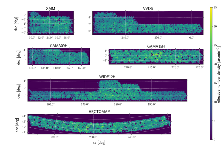
Figure 18: The effective galaxy number density map of the three-year HSC shape catalog. The map is a tangent projection of sky with a regular grid spacing of $1\arcmin$ after smoothing with a Gaussian kernel ($\sigma=1\farcs 5$). The arc feature is masked out by the “i$\_$pixelflags$\_$clipped $==$False” and “i$\_$pixelflags$\_$edge $==$ False” flags shown in Table 2, which is only obvious in HECTOMAP field due to the difference in the display resolution between the panels.

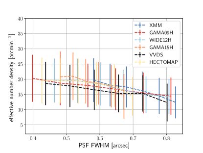
Figure 19: The mean effective galaxy number density (defined in Eq. (16)) of the catalog as a function of $i$-band PSF FWHM for each field. The errorbars denote the standard deviation of the effective number density in each PSF FWHM bin.

3.10 Blinding

Multiple cosmological analyses are being conducted by the HSC collaboration using the three-year HSC shear catalog, each with different analysis PIs. In order to avoid confirmation bias in cosmological analyses, we blind our catalog by adding a random additional multiplicative bias with a two-level blinding scheme (also see Hikage et al., 2019a). The first is a user-level blinding to prevent an accidental comparison of blinded catalogs between different analysis teams, while the second is collaboration-level blinding that is adopted in the cosmological analysis.

For the user-level blinding, we generate a random additional multiplicative bias $\mathrm{d}m_{1}$ for each catalog. The values of $\mathrm{d}m_{1}$ are different among different analysis teams, and they are encrypted with the public keys from the principle investigators (PIs) of the corresponding analysis teams. This single value of $\mathrm{d}m_{1}$ should be decrypted by the PI and subtracted from the multiplicative bias values for each catalog entry to remove the user-level blinding before the analysis.

For the collaboration-level blinding, we generate three blinded catalogs with indexes $j=0,1,2$. The additional multiplicative biases $\mathrm{d}m_{2}^{i}$ for these three blinded catalogs are randomly selected from the following three different choices of ($\mathrm{d}m_{2}^{1}$, $\mathrm{d}m_{2}^{2}$, $\mathrm{d}m_{2}^{3}$): $(-0.1,-0.05,0.)$, $(-0.05,0.,0.05)$, $(0.,0.05,0.1)$. In each case, the additional multiplicative biases are listed in an ascending order, while the true catalog has a different index for the three options. The values of $\mathrm{d}m_{2}^{1,2,3}$ are encrypted by a public key from one designated person who will not lead any cosmology analysis.

The final blinded multiplicative bias values for the galaxies in each catalog are modified as

$$m_{{\rm blind;i}}^{j}=m_{{\rm true;i}}+\mathrm{d}m_{1}^{j}+\mathrm{d}m_{2}^{j},$$ (17)

where $i$ is the galaxy index in each blinded catalog. Each PI receives a separate set of blinded catalogs, and carries out the same analysis for all three catalogs after decrypting and subtracting the $\mathrm{d}m_{1}$ from the multiplicative bias for each catalog.

We provide two types of blinded catalog. The one is the two-level blinding for cosmology analyses and the other is just user-level blinding for non-cosmology analysis. As we did for the first year weak lensing science, the additive bias is not blinded in weak lensing analyses.

4 Requirements on control of systematic uncertainties

In this section, we set requirements on the control of systematic residuals for the weak lensing shear catalog defined in Section 3.3. Note that the requirements can only be determined after the weak lensing galaxy sample is defined since the statistical errors that can be obtained from a cosmological analysis conducted with the shear catalog is the basis for setting meaningful requirements on the control of systematic residuals.

First, we forecast the statistical errors that are attainable with the shear catalog defined in Section 3.3. Similar to the first-year shear catalog, we will require the amplitude of each systematic residual $\delta X_{\text{sys}}$ for an observable denoted as $X$ (e.g., galaxy-shear cross correlation function or shear-shear correlation function) to contribute less than one-half of the statistical error on the observable, $\sigma_{X}$. That is,

$$|\delta X_{\text{sys}}|\lesssim 0.5\sigma_{X}\,.$$ (18)

We note that such a requirement is on the systematic residuals after the removal of known biases that are expected to be calibrated before the use of a catalog. We will assess the requirements in terms of multiplicative and fractional additive bias residuals (i.e., $\delta m$ and $\delta a$) in shear estimation, which are defined in Eq. (6).

Not all weak lensing science cases will require the same level of control of systematic residuals as we use in this paper, because some analyses will have lower SNR. The requirements defined here are tuned such that for certain key cosmological science cases, the statistical error will continue to dominate over the systematic residuals. When adding statistical and systematic errors in quadrature, this threshold would mean that ignoring the systematic residuals would result in an underestimation of the total uncertainty (statistical + systematic) by at most $12$ percent.

In this paper, we will check the magnitude of a number of systematics. If a particular systematic effect does not meet the requirements we set, the systematic residuals must be explicitly modeled and marginalized, potentially contributing a significant portion of the total error budget in the cosmological constraints. We also model and marginalize some of the systematics in our cosmological analyses even though they meet the requirements, to avoid a scenario where multiple residual systematic uncertainties that are each at the $0.5\sigma$ level combine such that the total systematic uncertainty dominates the final results.

4.1 Requirement from cosmic shear

Cosmic shear and galaxy-galaxy lensing are two of the most important scientific applications of the HSC shear catalog. They require measurements of the shear-shear correlations and the correlations between galaxy position and shear, respectively. The requirements on control of systematic residuals for galaxy-galaxy lensing are comparable to that for cosmic shear . Therefore, we will determine the requirements on systematic residuals using the expected covariance of shear-shear correlation functions. We estimate this by rescaling the covariance matrix, denoted as $\mathbf{C}$, of the first-year shear-shear correlations by the inverse square of the galaxy number ratio between the three-year catalog and the first-year catalog.

The shear-shear correlations are defined as

$$\xi_{\pm}(\theta)=\langle\hat{g}_{+}(\vec{r})\hat{g}_{+}(\vec{r}+\vec{\theta})\rangle\pm\langle\hat{g}_{\times}(\vec{r})\hat{g}_{\times}(\vec{r}+\vec{\theta})\rangle\,.$$ (19)

Here we decompose the per-object shear estimates $\hat{g}$ for pairs of galaxies into the tangential ($\hat{g}_{+}$) and cross component ($\hat{g}_{\times}$).

The first-year shear catalog paper (Mandelbaum et al., 2018a) used a covariance matrix measured from mock catalogs (Shirasaki et al., 2017, 2019) to estimate the SNR for a cosmic shear measurement without tomographic binning. The estimated SNR over angular scales $5\arcmin<\theta<285\arcmin$ is $12.6$. Cosmic shear analyses have been conducted using the first-year HSC shear catalog in both Fourier space (Hikage et al., 2019b) and configuration space (Hamana et al., 2020) with tomographic binning. The estimated SNRs of $15.6$ and $18.4$ were achieved with a fiducial multi-pole range $300<l<1900$ and an angular range $4\arcmin<\theta<50\arcmin$, respectively. The differences between the SNR measurements are mostly due to the different tomographic setups, angular ranges and cosmological models adopted by these studies. Here we take their average and rescale it according to the increase in galaxy number. This process yields a rescaled SNR${}_{s-s}=27$. Note that even though we consider tomographic SNR measurements when deriving SNR_s-s, we adopt a non-tomographic formalism when deriving the requirements in the following context for simplicity.

We use this SNR to derive the upper limit of the amplitude of systematic residuals on the cosmic shear as

$$\delta\xi_{\pm,\text{max}}(\theta)=\frac{\xi_{\pm}(\theta)}{2\,\text{SNR}_{s-s}},$$ (20)

which has a statistical significance of $0.5\sigma\,$. In summary, the requirement on the amplitude of systematic residuals that originate from any sources on the cosmic shear measurement is given by

$$|\delta\xi_{\pm}|<\delta\xi_{\pm,\text{max}}\,.$$ (21)

4.2 Multiplicative bias residuals

In this section, we place a requirement on the overall residual multiplicative shear bias ($\delta m$) after the calibration process described in Section 3.5. To focus on multiplicative bias residuals, we consider the situation that the additive bias is zero. If we neglect the high-order terms of $\delta m$ with the assumption that $\delta m\ll 1$, the multiplicative bias residual primarily affects the shear-shear correlations as

$$\langle\hat{g}^{\dagger}\hat{g}\rangle\approx(1+2\,\delta m)\langle g^{\dagger}g\rangle,$$ (22)

where $g^{\dagger}$ refers to the complex conjugate of $g$. The systematic residual on the correlation function due to the multiplicative bias residual is

$$\delta\xi_{+,\delta m}=2\,\delta m\,\xi_{+}\,.$$ (23)

According to Eq. (21), the value of $2|\delta m|$ should be $\lesssim 0.5/\text{SNR}_{\text{s-s}}$, or

$$|\delta m|\lesssim\frac{0.25}{\text{SNR}_{\text{s-s}}}=9.3\times 10^{-3}\,.$$ (24)

with integrated SNR (SNR${}_{\text{s-s}}=27$) for cosmic shear. This requirement is $\sim\sqrt{3}$ times as stringent as the first-year requirement on the multiplicative bias.

4.3 PSF model size errors

The systematic residual on PSF model size is quantified by the fractional PSF size residual:

$$f_{\delta\sigma}=\frac{\delta\sigma_{\text{PSF}}}{\sigma_{\text{PSF}}},$$ (25)

where $\sigma_{\text{PSF}}$ is the determinant radius calculated from the second moments of the PSF. Such systematics lead to an additive shift in the shear-shear correlation function $\xi_{+}(\theta)$ (Jarvis et al., 2016), which can be written as

$$\delta\xi_{+,\delta\sigma}=4\langle f_{\delta\sigma_{\text{PSF}}}\rangle\xi_{+}(\theta),$$ (26)

if we use the approximation: $\langle T_{\text{PSF}}/T_{\text{gal}}\rangle=1$, and set the fractional PSF model area (trace) error to twice the fractional PSF determinant radius error (Mandelbaum et al., 2018a).

Therefore, we place a specific requirement on the PSF model size errors – the systematics should be less than $0.5|\delta\xi_{\pm}|$ – as we did in Mandelbaum et al. (2018a). With the integrated SNR ($\text{SNR}_{\text{s-s}}=27$), the requirement is written as

$$|\left\langle f_{\delta\sigma}\right\rangle|\lesssim\frac{1}{16\,\text{SNR}_{\text{s-s}}}\approx 2.3\times 10^{-3}\,.$$ (27)

This requirement is also $\sim\sqrt{3}$ times as stringent as the first-year requirement on the PSF model size errors.

4.4 Additive bias residuals

In this section, we place a requirement on the correlation of the overall additive shear bias residual ($\delta c$), originating from, e.g., an inadequate removal of PSF anisotropy in the shear estimation or the PSF model shape errors, etc. Similar to Section 4.2, we set $\delta m=0$ to focus on the additive bias residual ($\delta c$). The additive bias ($c$) propagates into an additive term in the correlation function through

$$\langle\hat{g}^{\dagger}\hat{g}\rangle=\langle g^{\dagger}g\rangle+\langle\delta c^{\dagger}\delta c\rangle\,.$$ (28)

Then the systematic residual that originates from additive bias residual is given by

$$\delta\xi_{+,\delta c}=\langle\delta c^{\dagger}\delta c\rangle\,.$$ (29)

According to Eq. (21) and the conservative integrated SNR (SNR${}_{\text{s-s}}=27$), the requirement on the correlation of fractional additive bias is

$$\begin{split}\langle\delta c^{\dagger}\delta c\rangle&<\frac{\xi_{+}(\theta)}{2\,\text{SNR}_{\text{s-s}}}\\ &=\frac{\xi_{+}(\theta)}{54}.\end{split}$$ (30)

Using the relation $\delta c=\delta a\,e_{\text{PSF}}$, we transform the requirement on $\langle\delta c^{\dagger}\delta c\rangle$ to the requirement on $\langle\delta a\,\delta a\rangle$:

$$\langle\delta a\,\delta a\rangle<\frac{\xi_{+}(\theta)}{54\langle e^{\dagger}_{\text{PSF}}e_{\text{PSF}}\rangle(\theta)}\,.$$ (31)

Note , when using $\delta c=\delta a\,e_{\text{PSF}}$, we neglect the PSF model shape errors, the requirement of which will be quantified in Section 4.5.

In order to use the cosmic shear signals at scales where baryonic effects are unimportant, we only consider the $\xi_{+}$ measurements on scales from $4\arcmin$ to $50\arcmin$ as in Hamana et al. (2020). The quantity $\langle\delta a\,\delta a\rangle$ declines as a function of angular scale, ranging from $\sim 2.0\times 10^{-4}$ at our minimum scale of $\theta=4\arcmin$ to $\sim 4.3\times 10^{-5}$ at $\theta=50\arcmin$ since the scale-dependence of the PSF-PSF shape correlation (denominator) is much flatter than that of the cosmic shear correlation function (numerator). As we have already conservatively used the integrated SNR in this equation, it is not necessary to use the lowest $\langle\delta a\,\delta a\rangle$ value as well; rather, we use the geometric mean of these values, requiring $|\delta a|^{2}<9.4\times 10^{-5}$, or $|\delta a|<9.7\times 10^{-3}$.

4.5 PSF model shape errors

Systematic correlations in the errors in the shape of PSF model, which are quantified by the PSF model shape residual ($\delta g_{\text{PSF}}$), also produce an additive term in the galaxy shear-shear correlations. Here we place a requirement on the spatial correlations of PSF model shape errors by requiring the additive terms induced by PSF shape errors to be half the statistical error (Mandelbaum et al., 2018a).

The additive terms are expressed in Eq. (3.17) in Jarvis et al. (2016), which depends on the five $\rho$ statistics, two of which were defined in Rowe (2010) and the last three in Jarvis et al. (2016). The $\rho$ statistics are summarized as follows:

$$\rho_{1}(\theta) \equiv\left\langle\delta g_{\text{PSF}}^{\dagger}(\vec{r})\delta g_{\text{PSF}}(\vec{r}+\vec{\theta})\right\rangle,$$ (32)

$$\rho_{2}(\theta) \equiv\left\langle g_{\text{PSF}}^{\dagger}(\vec{r})\delta g_{\text{PSF}}(\vec{r}+\vec{\theta})\right\rangle,$$ (33)

$$\rho_{3}(\theta) \equiv\left\langle\left(g_{\text{PSF}}^{\dagger}\frac{\delta T_{\text{PSF}}}{T_{\text{PSF}}}\right)(\vec{r})\left(g_{\text{PSF}}\frac{\delta T_{\text{PSF}}}{T_{\text{PSF}}}\right)(\vec{r}+\vec{\theta})\right\rangle,$$ (34)

$$\rho_{4}(\theta) \equiv\left\langle\delta g_{\text{PSF}}^{\dagger}(\vec{r})\left(g_{\text{PSF}}\frac{\delta T_{\text{PSF}}}{T_{\text{PSF}}}\right)(\vec{r}+\vec{\theta})\right\rangle,$$ (35)

$$\rho_{5}(\theta) \equiv\left\langle g_{\text{PSF}}^{\dagger}(\vec{r})\left(g_{\text{PSF}}\frac{\delta T_{\text{PSF}}}{T_{\text{PSF}}}\right)(\vec{r}+\vec{\theta})\right\rangle.$$ (36)

$\rho_{1}$ is the auto-correlation function of PSF model shape residuals, while $\rho_{2}$ is its cross-correlation with the PSF shape itself. The other statistics, i.e., $\rho_{3,4,5}$, involve $T_{\text{PSF}}$ – the trace of the second moment matrix of the PSF.

We place requirements on the $\rho$ statistics following Eqs. (33)–(34) of Mandelbaum et al. (2018a) using the conservative integrated SNR (SNR${}_{\text{s-s}}$) to avoid a binning-dependence of the requirement. These requirements become

$$\begin{split}|\rho_{1,3,4}(\theta)|<\frac{\xi_{+}(\theta)}{2\,\text{SNR}_{\text{s-s}}}=\frac{\xi_{+}(\theta)}{54},\\ |\rho_{2,5}(\theta)|<\frac{\xi_{+}(\theta)}{4|\delta a|\,\text{SNR}_{\text{s-s}}}=\frac{\xi_{+}(\theta)}{108|\delta a|},\end{split}$$ (37)

where $\delta a$ is the remaining fractional additive bias due to the leakage of PSF anisotropy into the shear estimation after the calibration with image simulations. Here we set $\delta a$ to $0.02$, which is greater than the value we detect in Section 3.6, to ensure that our requirement is stringent enough for the weak lensing science.

5 PSF Model Tests

In this section, we carry out tests to ascertain the fidelity of the PSF modelling for $i$-band coadds. In Section 5.1, we define the star samples used for PSF tests. In Section 5.2, we select regions where PSF adequately modeled. We test the PSF model size and PSF model shape residuals in Section 5.3 and Section 5.4.

5.1 Star sample

In the HSC pipeline, the PSF modelling is carried out with a modified version of PSFEx (Bertin, 2011) at the single exposure level after correction for the brighter-fatter effect (Coulton et al., 2018). The PSFs on coadded images are reconstructed based on coaddition of the PSF models estimated in each CCD visit by interpolating star images. The selection of stars used for PSF modelling is based on the k-means clustering of high-SNR (i.e., SNR$>50$) objects in size, typically resulting in $\sim 80$ star candidates per CCD chip with an area of $\sim 60$ arcmin² (see Bosch et al. 2018 for details). At the single exposure CCD processing, $\sim 20\%$ of the stars in a given single exposure are randomly selected and reserved for cross-validation and are not used for PSF modelling. Since the star sample used in PSF modelling is derived on individual exposures, different exposures will not necessarily select the same set of stars. At the coadded image level, stars that were used by $\geq 20\%$ of the input visits is labelled as having been used in the modeling, namely “i$\_$calib$\_$psf$\_$used$==$True”.

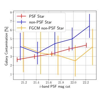
Figure 20: The galaxy fractions misclassified as stars in three star catalogs (i.e., PSF-star, non-PSF star, and FGCM non-PSF star) as a function of $i$-band PSF magnitude cut at the faint end. The results are estimated with a reference to the COSMOS HST star-galaxy classifications as ground truth. Errorbars show the Poisson uncertainties.

The systematic tests are conducted at the coadded image level. The star sample used in the tests is selected by “i$\_$extendedness$\_$value$==0$”, which is a cut indicating whether an object is extended (galaxy) or point-like (star) as shown in Table 2. Following Mandelbaum et al. (2018a), a $22.5$ magnitude cut in $i$-band is applied to select a high-SNR star sample. In this magnitude limited star sample, those flagged by “i$\_$calib$\_$psf$\_$used $==$ True” are defined as PSF stars, and the others are defined as non-PSF stars. We match these star samples in the COSMOS region to the HST catalog of Leauthaud et al. (2007), and use the HST galaxy-star classification as a reference to estimate the galaxy contamination in our star catalogs. Fig. 20 shows the estimated galaxy contamination as a function of $i$-band PSF magnitude limit. As shown, the fraction of galaxy contamination is smaller by $\sim 2\%$ in PSF-star sample than in non-PSF star sample for the $22.5$th magnitude cut. This is because “i$\_$calib$\_$psf$\_$used $==$ True” is a stricter selection of stars based on both size and brightness information. In contrast, “i$\_$extendedness$\_$value$==0$” selects stars only based on size information.

In order to further improve the purity of the non-PSF stars and reduce the contamination by galaxies, we cross-match this star sample to the star catalog selected from the HSC S20A data release (Aihara et al., 2021) for the Forward Global Calibration Method (FGCM; Burke et al., 2018) photometry calibration by their sky coordinates. Hereinafter, we term this cross-matched star catalog as FGCM non-PSF stars. The number of PSF stars, non-PSF stars and FGCM non-PSF stars are $2260229$, $186529$, and $87131$, respectively. As shown in Fig. 20, the purity of this FGCM non-PSF stars is better than non-PSF stars and comparable to PSF stars for the 22.5th magnitude cut. This is because the FGCM selection requires each star in the catalog to be identified as point-like sources in at least two observations (not limited to $i$-band) in the single exposure image processing. In addition, the FGCM star catalog is downsampled for a homogeneous distribution on the sky. We refer readers to Aihara et al. (2021) for more detailed description of the FGCM star catalog.

To quantify the fidelity of the PSF reconstruction we perform tests of the PSF size and shape residuals. Using the image of a star on coadded images as a proxy for the true PSF, the fractional PSF model size residual ($f_{\delta\sigma}$) can be quantified as

$$f_{\delta\sigma}=\frac{\sigma_{\text{PSF}}-\sigma_{\text{*}}}{\sigma_{*}},$$ (38)

and the PSF model shape residual ($\delta g_{\text{PSF}}$) is quantified as

$$\delta g_{\text{PSF}}=g_{*}-g_{\text{PSF}},$$ (39)

where $\sigma_{*}$ ($g_{*}$) is the size (shape) of the star, and $\sigma_{\text{PSF}}$ ($g_{\text{PSF}}$) is the PSF model size (shape) evaluated at the position of the star.

5.2 PSF region cut

In the first-year shear catalog, significant PSF model size residuals were identified in the VVDS region, which included some of the “very best seeing” data with PSF FWHM less than $0\farcs 5$ (see Fig. 9 of Aihara et al. 2019). As described in Section 2, in the current data release, the improved PSF interpolation for small-size PSFs as detailed in Aihara et al. (2019) has ameliorated this issue. Therefore, unlike the first-year shear catalog (Mandelbaum et al., 2018a), we do not remove the “very best seeing” regions.

However, we do perform a cut since we find the histogram of the fractional size residuals is skewed toward positive. In addition, the cut is applied to ensure that the PSF model size is adequately modeled in the selected regions. To suppress measurement noise, we average the fractional size residuals ($f_{\delta\sigma}$) within each HEALPix pixel with ${\tt NSIDE}=1024$ corresponding to an area of $\sim 12\ {\rm arcmin}^{2}$. The number of PSF stars in a HEALPix pixel varies from $\sim 10$ to $\sim 24$. We then plot the average fractional size residual (Eq. (38)) as a function of average seeing within the corresponding HEALPix pixels in Fig. 21. We limit the weak lensing FDFC (WLFDFC) region to HEALPix pixels with $\langle f_{\delta\sigma}\rangle<0.01$. This cut reduce the PSF model size residuals on average while only removing $\sim 2.2\%$ of the FDFC region.

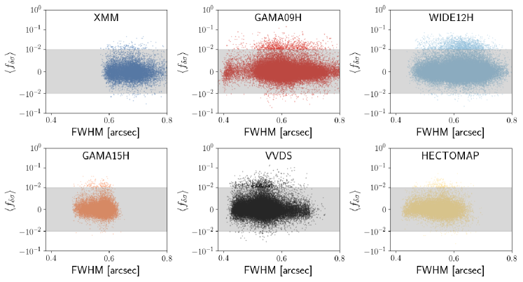
Figure 21: The average fractional size residual $\langle f_{\delta\sigma}\rangle$ reconstructed at star positions, averaged over the PSF stars within HEALPix pixels with ${\tt NSIDE}=1024$, and shown as a function of seeing. A symlog scale is used to allow negative residuals to be shown. The gray region indicates the linear part of the symlog scale, with the rest being logarithmic. The upper boundary of the gray regions are the fractional size cut ($f_{\delta\sigma}<0.01$) we apply to remove the HEALPix pixels with large positive amplitude of size residual.

5.3 PSF model size

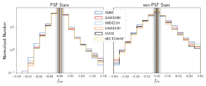
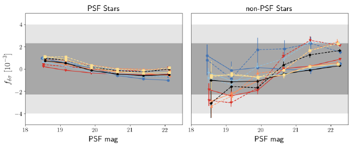
Figure 22: Upper left: Distribution of the fractional size residual ($f_{\delta\sigma}$) for PSF stars in each field. The dark- (light-)gray region indicate the requirements on the residual for the three- (first-)year shear catalog. The vertical dashed (solid) lines show the mean (median) of $f_{\delta\sigma}$. Upper right: Same as the upper left, but for FGCM non-PSF stars. Lower left: $f_{\delta\sigma}$ as a function of the $i$-band PSF magnitude for PSF stars in each field. The dark- (light-)gray region indicates the three- (first-)year requirement. The dashed (solid) lines show the mean (median). Lower right: Same as lower left, but for FGCM non-PSF stars.

The results of the PSF model size residual tests are shown in Fig. 22. The two plots in the upper panels are the number distributions of $f_{\delta\sigma}$ for PSF stars (left) and FGCM non-PSF stars (right). Here we show the mean and median for each field and compare with the overall three-year requirement. All of the results are well within the three-year requirement. Compared to the PSF stars, the results (mean and median) for FGCM non-PSF stars have slightly larger deviations from zero. The deviation in the mean values is more pronounced compared to that in the median, as the mean value is more sensitive to the outliers and/or the skewness of the distribution.

The two lower panels show fractional size residuals as a function of PSF magnitude. The lower left panel shows the mean (solid lines) and median (dashed lines) for PSF stars (Bosch et al., 2018). The lower right panel shows the results of FGCM non-PSF stars. The magnitude dependence of the mean size residual for FGCM non-PSF stars is slightly different from that of PSF stars. The results of FGCM non-PSF stars are within our requirements, except perhaps at the bright and the faint ends of the magnitude bins in the WIDE12H and GAMA09H fields. However, given the large size of the uncertainties, the evidence for the difference between the PSF stars and the FGCM non-PSF stars is not entirely conclusive.

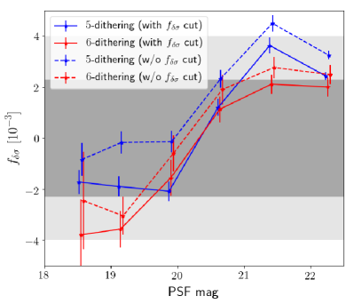
Figure 23: The fractional size residual of FGCM non-PSF stars from the WIDE12H field divided into the $5$-dithering regions (blue lines) and the $6$-dithering regions (red lines) as a function of $i$-band PSF magnitude. The dashed lines and solid lines represent the results with and without $\langle f_{\delta\sigma}\rangle<0.01$, respectively. The gray region indicate the requirements on the residual for the three-year shear catalog. Results are shifted horizontally for illustrative purposes.

As described in Section 2.5, the dithering strategy was changed in S19A from a $6$-dithering pattern to a $5$-dithering pattern in the $i$-band. Thus the definition of the FDFC region has also been changed as described in Section 2. To assess the impact of this change in observing strategy on PSF modelling quality, we have tested the PSF modelling from regions with different dither patterns. Here we show the results of the WIDE12H field as an example, where we contrast the PSF model size residuals in a patch with a $6$-dithering pattern to that observed in patches with a 5-dithering pattern. As illustrated by the color map of numbers of input visits in Fig. 3, the central patch of the WIDE12H field with redder color corresponds to the region with the $6$-dithering pattern, with $174\fdg 0\leq\text{ra}<190\fdg 5$ and $\text{dec}<=1\fdg 6$. The other three patches surrounding the central region correspond to the $5$-dithering pattern.

Fig. 23 shows $\langle f_{\delta\sigma}\rangle$ as a function of the star magnitude from the aforementioned $6$-dithering region and the $5$-dithering region in WIDE12H field with/without the $\langle f_{\delta\sigma}\rangle<0.01$ cut. WIDE12H field is used to test the different dithering region because it has much larger $5$-dithering region than the other fields. We observe small differences between the $6$-dithering region and the $5$-dithering region. At the bright end, $f_{\delta\sigma}$ is slightly lower than the lower boundary of the requirement for the $6$-dithering region, while it is slightly above the upper boundary of the requirement for the $5$-dithering region. The results of both of the dithering strategies slightly improve after applying the cut on $f_{\delta\sigma}$.

The correlation function of the fractional size residual ($f_{\delta\sigma}$) for each field is shown in Fig. 24. Comparing with the results of the first-year shear catalog shown in the lower right panel of Fig. 6 in Mandelbaum et al. (2018a), we conclude that although the three-year results show scale dependence and the first-year results demonstrate weaker scale dependence, the amplitudes are much lower. The correlations have decreased by a factor of $\sim$10 at $1\degree$ scale and a factor of $\sim$2 at $0.1\degree$ scale compared to what was seen in the first-year shear catalog.

5.4 PSF model shape

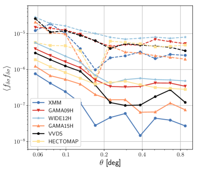
Figure 24: The star fractional size residual ($f_{\delta\sigma}$) correlation for PSF stars (solid lines) and FGCM non-PSF stars (dashed lines) in each field.

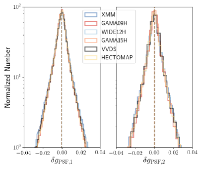
Figure 25: Distribution of PSF model shape residual ($\delta g_{\text{PSF}}$) for the FGCM non-PSF stars in each field. The vertical lines show the average of $\delta g_{\text{PSF}}\,$.

The PSF model shape residual distributions for both PSF and FGCM non-PSF stars are shown Fig. 25. We plot the median and mean of the distribution of each field. We do not place a requirement on the average of shape residuals since the average additive bias from PSF model shape errors can be removed by cross-correlating with a random catalog that has the same area coverage as the lens sample for galaxy-galaxy lensing measurements, and we directly place requirements on the correlations of the PSF model shape errors for cosmic shear measurements.

In Fig. 26, we show the $\rho$ statistics, defined in Eqs. (33)–(36) which are constructed from the spatial correlation functions of PSF model shape and size residuals. The requirements on the $\rho$ statistics discussed in Section 4.5 are shown by the dark-gray regions in all the panels. On all $\rho$ statistics, we show the results for PSF stars (black points) and FGCM non-PSF stars (red points). In order to avoid the potential difference in the $\rho$ statistics between the PSF stars and the FGCM non-PSF stars due to the population difference between these two star samples caused by the SNR cut in the PSF star selection, we perform a reweighting of the FGCM non-PSF stars so that they match the magnitude distribution of the PSF stars. The $\rho_{2}$–$\rho_{5}$ statistics are generally within the three-year requirements at scales $\theta<1^{\circ}$, regardless of the noisiness of these statistics for the FGCM non-PSF stars due to their small numbers. We observe some flattening in the $\rho_{2}$ statistics on scales nearing the size of the field of view of our camera. Similar issue can be seen in the top left panel, where there is some evidence that $\rho_{1}$, which is the auto-correlation of the PSF shape residuals, marginally exceeds the requirements on scales greater than $50\arcmin\,$. Another concern is the $\rho_{1}$ statistic for the FGCM non-PSF stars. Although it is noisy, the $\rho_{1}$ statistic is at the very edges of our three-year requirements. In addition, we have confirmed that whether applying the aforementioned reweighting processing to match the magnitude distributions or not does not change the conclusion.

In the cosmic shear analyses, this particular systematic and its impact on the cosmological inference needs to be carefully accounted for (see e.g., the treatment in Hikage et al., 2019a; Hamana et al., 2020; Amon et al., 2021). Similarly large values for the $\rho_{1}$ statistic were seen in the DES year 1 data (Zuntz et al., 2018) and are likely related to the use of PSFex for modeling the PSF. In DES year 3 data, this issue was significantly reduced by the use of a new PSF extraction software called PIFF (PSFs In the Full FOV) introduced in Jarvis et al. (2021). The implementation of PIFF in the LSST pipeline (and subsequently the HSC pipeline) is currently in progress and future releases of the shape catalog from HSC are likely to include these improvements.

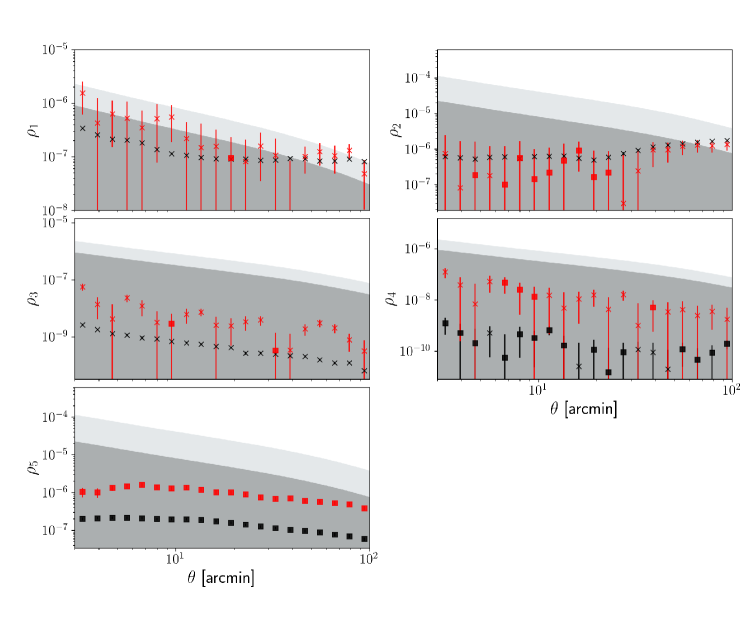
Figure 26: PSF model shape residual correlations, or $\rho$ statistics, $\rho_{1}$ through $\rho_{5}$ (defined in Section 4.5) as a function of separation $\theta$ on the sky. Negative values are shown in absolute values and denoted by ‘$\mathbin{\text{\char 13\relax}}$’, whereas positive values are shown as they are and denoted by ‘$\times$’. Black (red) points are for PSF stars (FGCM non-PSF stars). The regions with dark- (light-)gray background are within the three- (first-)year HSC requirement. The errorbars are estimated by bootstrap resampling.

6 Null Tests

In this section, we conduct internal null tests related to galaxy and star shapes within the shear catalog. We first show the mean shear value as functions of different galaxy properties in Section 6.1. Then we cross-correlate galaxy shapes with positions (e.g., stars and random positions) in Section 6.2. Subsequently, we test the systematics related to mass map reconstruction in Section 6.3. Finally, we cross-correlate galaxy shapes with star shapes to test the systematics related to PSF revision and PSF model errors in the shear estimation.

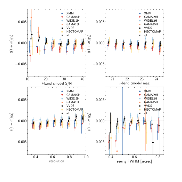
Figure 27: Weighted mean shear values $\langle g_{1}\rangle$ as a function of $i$-band CModel SNR (top-left), $i$-band CModel magnitude (top-right), the reGauss resolution factor corresponding to galaxy size (bottom-left), and PSF FWHM (bottom-right). Errorbars are the $1\sigma$ uncertainties estimated from mock shear catalogs and include cosmic variance.

6.1 Mean shear values

We first calculate the mean shear $\langle g_{1}\rangle$ and $\langle g_{2}\rangle$, which is sensitive to any additive bias residual that is independent of the PSF ellipticity. Throughout the paper we derive mean shear values in sky coordinates, which are quite close to the CCD coordinates in most cases. To check whether the mean shear values are dominated by systematic errors, we derive uncertainties on those mean shear values from mock shear catalogs including both shape noise and cosmic variance from $N$-body simulations. Specifically, we create $200$ realizations of mock catalogs following the method described in Oguri et al. (2018) (also see Shirasaki et al., 2019), which adopts ray-tracing results of Takahashi et al. (2017). We derive the $p$-value for a fit to zero signal for the weighted mean value of each shear component in the six fields. We find that only one of the 12 $p$-values is below a nominal threshold of 0.05, with an $p$-value of $0.024\,$. We therefore conclude that the mean shear values do not exhibit signs of significant systematic errors.

Following Mandelbaum et al. (2018a), we also check weighted mean shear values $\langle g_{1}\rangle$ as a function of four properties of the $i$-band images: CModel SNR, CModel magnitude, the reGauss resolution parameter corresponding to galaxy size, and the PSF FWHM. The error for the PSF FWHM bin at $\sim 0\farcs 5$ in XMM field blows up due to the limited galaxy number in this bin as shown by the number histogram in Fig. 4. Results for all fields combined, as shown in Fig. 27, indicate that most of mean shear values are consistent with zero within $2\sigma$. Moreover, the average shear values do not show strong dependence on these galaxy properties, although the average shear values for some observational fields are persistently positive or negative in almost all galaxy property bins this is very likely due to the bin-to-bin correlations, ranging from $0.3$ to $0.6$ (Mandelbaum et al., 2018a), caused by cosmic variance.

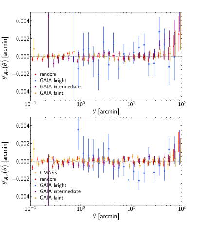
Figure 28: Stacked tangential (upper) and cross (lower) shear profiles, averaged over the entire survey, around the CMASS galaxy sample (inverted triangles), random points (triangles), bright Gaia stars with $G<10$ (squares), intermediate Gaia stars with $13<G<14$ (pentagons), and faint Gaia stars with $18<G<18.2$ (circles). Only cross shear profiles are shown for stacking around CMASS galaxies. Errors are estimated from mock shear catalogs including cosmic shear. The $\chi^{2}$ and $p$ values are summarized in Tables 4 and 5 in Appendix A.

6.2 Stacked shear signals

When measuring stacked shear signals for a source sample in annuli around a sample of massive lenses, the stacked cross (not tangential) shear signals should be zero due to symmetry (e.g., Massey et al., 2007a). This fact therefore provides a useful null test. In addition, stacked tangential shear signals around objects that do not induce any weak lensing signals (e.g., stars and random positions, etc.) can also be used for null tests. In this subsection we explore stacked shear profiles around the following objects:

1. We adopt the CMASS galaxy sample of the SDSS-III Baryon Oscillation Spectroscopic Survey Data Release 12 (Reid et al., 2016b) with an additional redshift cut of $0.4<z<0.7$. The galaxy density is about 90 deg^-2. Since the tangential shear profiles around CMASS galaxies have clear positive signals, we only use the cross shear profiles for our null tests.

2. We use random points generated in the HSC-SSP footprint with a density of 100 deg^-2. In this case, we use both tangential and cross shear profiles for our null tests.

3. We use star catalogs generated from the Gaia Data Release 2 data (Gaia Collaboration et al., 2018), which is currently used to create bright star masks for the HSC-SSP data (Aihara et al., 2019). We use the Gaia bright, intermediate, and faint star catalogs consisting of Gaia stars with $G$-band magnitude $G<10$, $13<G<14$, and $18<G<18.2$, respectively, and use these three catalogs for our null tests. Bright stars are suitable for testing the validity of our bright star masks and the impacts of background residuals near bright stars on the shape measurements, whereas faint stars are suitable for testing the effect of possible residual systematics of the PSF correction in shape measurements.

Fig. 28 summarizes results of our null tests from stacked shear signals averaged over the entire survey area. We find that the shear profiles are mostly consistent with zero, suggesting no evidence for any significant detection of systematic effects. To quantify the significance of any deviations from zero, in Tables 4 and 5 in Appendix A, we tabulate $\chi^{2}$ and $p$ values for the null hypothesis of the stacked shear profiles for the six individual fields as well as all fields combined. To do so, we fully account for correlations between different radial bins, which are caused by e.g., cosmic shear, by deriving the full covariance matrix of the measurements using the 200 realizations of the mock shear catalog mentioned above. We include the correction factor ($\sim 0.85-0.9$) of Hartlap et al. (2007) to correct the covariances estimated from a limited number of realisations. We find that only four out of 63 $p$ values fall below a nominal threshold of 0.05, which is consistent with statistical fluctuations. Therefore we conclude that stacked shear profile tests show no significant evidence for significant systematic errors in the shear catalogs.

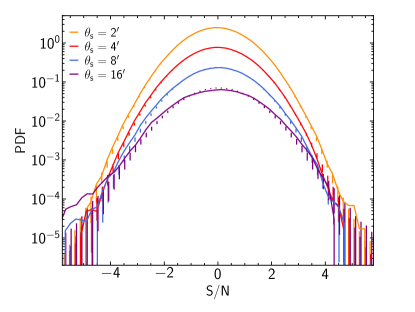
Figure 29: Observed $B$-mode mass map probability distribution functions (PDFs) for different smoothing length $\theta_{\rm s}$, which are shown by solid lines, are compared with those from mock shear catalogs with errors shown by bars. Results for $\theta_{\rm s}=2^{\prime}$, $4^{\prime}$, and $8^{\prime}$ are shifted upward by 1.5 dex, 1 dex, and 0.5 dex, respectively, for illustrative purposes.

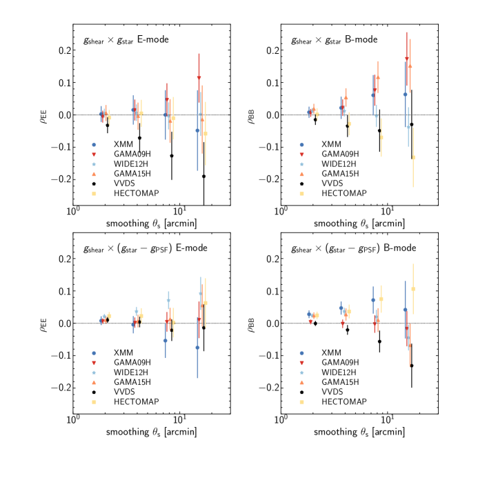
Figure 30: Pearson cross-correlation coefficients of $E$- (left panels) and $B$-mode (right panels) mass maps and star mass maps constructed using star ellipticities. We consider cases both with (lower panels) and without (upper panels) the PSF correction for star mass maps. Pearson cross-correlation coefficients are shown as a function of the smoothing length of mass maps. Different symbols show results for different observed fields. Errors are estimated from mock shear catalogs including cosmic shear.

6.3 Mass maps

The observed shear field can be converted to the projected density field (Kaiser & Squires, 1993). Since weak lensing produces mostly “$E$-mode” convergence fields, we can use “$B$-mode” convergence fields as additional null tests. For this purpose, we reconstruct Gaussian-smoothed convergence maps adopting four different smoothing lengths, following the methodology detailed in Oguri et al. (2018). Fig. 29 shows the PDFs of the $B$-mode mass maps for four different smoothing lengths as compared to the average PDFs from mock shear catalogs that correctly capture effects of the survey boundary and masking that mix $E$- and $B$-modes. We find that the $B$-mode mass map PDFs follow an approximately Gaussian distribution and are roughly consistent with those from mock shear catalogs. There are small deviations from the mock results, which were also seen in the HSC-SSP S16A shear catalog (Mandelbaum et al., 2018a) and must originate from PSF leakage or PSF modelling errors as we will discuss below.

Mass maps can be used for a complementary check for PSF leakage and PSF modelling errors (see e.g., Mandelbaum et al., 2018a). Specifically, we derive the Pearson correlation coefficient $\rho_{\kappa_{1}\kappa_{2}}$ between the $E$- or $B$-mode mass map and the $E$- or $B$-mode star mass map, where the star mass map refers to the smoothed convergence map created using star ellipticities. We consider two types of star ellipticities: one uses observed star ellipticities to check for PSF leakage, and the other uses star ellipticities after PSF correction to check for PSF modelling errors. In this analysis, we only use reserved stars that are not used for modelling the PSF. We show the results in Fig. 30. We find that correlations between mass maps and star mass maps without the PSF correction are consistent with zero within $\sim 2\sigma$, indicating that this test shows no sign of PSF leakage. On the other hand, we see small deviations from zero for the case of star mass maps with the PSF correction, which suggests that PSF modelling errors may be a source of small deviations of the $B$-mode mass map PDFs from mock results as shown in Fig. 29. This likely has a similar origin as that of the issue related to the $\rho_{2}$ statistic on large scales seen in Fig. 26 in Section 5. These PSF effects and their impact need to be carefully evaluated during cosmological analyses as was done in Hikage et al. (2019b) and Hamana et al. (2020).

6.4 Star-galaxy cross correlation

Next, following Mandelbaum et al. (2018a), we present results of an empirical test for the possible impact of either PSF modelling errors or residual PSF anisotropy in galaxy shapes on cosmic shear two-point correlation function measurements. We calculate the following combination of the star-galaxy cross correlation function and the star auto correlation function,

$$\xi_{\rm sys}=\frac{\langle g^{\dagger}_{\ast}\hat{g}_{\rm gal}\rangle^{2}}{\langle g^{\dagger}_{\ast}\hat{g}_{\ast}\rangle}.$$ (40)

Adopting the prescription given in Section 4.4, one finds that this combination gives an estimate of a residual correlation caused by PSF anisotropy leakage to the galaxy-galaxy correlation function ($\langle g^{\dagger}g\rangle$), $\Delta\langle g^{\dagger}g\rangle\sim a^{2}\langle g^{\dagger}_{\ast}g_{\ast}\rangle$. Note that $\xi_{\rm sys}$ can also detect additive PSF modelling errors that contribute to $\langle g^{\dagger}g\rangle$. Fig. 31 shows $\xi_{\rm sys}$ for each field along with the standard $\Lambda$CDM prediction of $\xi_{+}$, the cosmic shear correlation function. Overall, the amplitudes and shapes of $\xi_{\rm sys}$ are similar to those of the first-year shear catalog (see Fig. 18 of Mandelbaum et al. 2018a). The amplitude of $\xi_{\rm sys}$ varies among fields and can be comparable to $\langle g^{\dagger}g\rangle$ on degree scales. This indicates that a careful choice of angular scales used in cosmological analyses of cosmic shear two-point correlation function (or power spectrum) and a correction for the impact of PSF errors are required, as was done in Hikage et al. (2019a) and Hamana et al. (2020).

Figure 31: Separate panels show (for each survey field) the shape–shape correlation function $\xi_{+}(\theta)$ for PSF star shapes as points (the errors are smaller than the size of the points); the predicted cosmic shear correlation function with a WMAP9 cosmology using the $n(z)$ from HSC photometric redshifts without any correction for photo-$z$ errors (which illustrates the approximate magnitude of the expected cosmic shear signal) as dashed lines; and $\xi_{\rm sys}$, defined in equation (40), as crosses.

7 Summary and Outlook

In this paper, we presented the galaxy shear catalog measured from the $i$-band wide layer of the HSC S19A internal data release. The galaxy shapes were calibrated with HSC-like image simulations that transfer the galaxy images from COSMOS HST to the HSC observing conditions. We confirmed that the simulated galaxy sample has the same distributions of galaxy properties as the real HSC data. Then we used the simulation to calibrate the galaxy property-dependent shear estimation bias, including redshift-dependent bias. We tested the residuals of the shear calibration by applying the calibrated shear estimator to sub-samples of the simulation divided by several different galaxy properties. The selection bias was removed empirically from ensemble shear estimates using the simulation.

In summary, the resulting galaxy shear catalog covers an area of $433.48~{}\rm{deg}^{2}$ of the northern sky, split into six fields, with a mean $i$-band seeing of $0.59\arcsec$. With conservative galaxy selection criteria, the raw galaxy number density is $22.9~{}\rm{arcmin}^{-2}$ and the effective galaxy number density is $19.9~{}\rm{arcmin}^{-2}$. The galaxy catalog has a depth of $24.5$th magnitude.

We defined the requirements for cosmological weak lensing science for this shear catalog, and quantified potential systematics in the catalog using a series of internal null tests for problems with point-spread function modelling and shear estimation.

7.1 Future improvements

Here we summarize the areas to improve in our future shear catalog, beyond the already-highlighted issue of PSF model shape residuals (Section 5).

7.1.1 Shear catalogs from multi-band images

One limitation of our current shear catalog is that we only have $i$-band image simulations to validate and calibrate shear estimations obtained from $i$-band. That is, we are not able to use the galaxy shapes observed from other filter bands to reduce shape measurement uncertainties and shape noise in weak lensing science. The potential difficulty that need to be overcome to generate shear catalogs from multi-band HSC images is that other bands (i.e., $grzy$) are different in wavelength from F814W band filter, the transmission curve of which has a much larger overlap with that of the $i$-band filter than other bands. Therefore, it would be necessary to carefully check whether the input training samples are still representative of the galaxy images in other bands of HSC.

7.1.2 Unrecognized blending

Unrecognized blending refers to the case that multiple blended sources are identified as one single source by the detector. It has been shown by many existing works that unrecognized blending has two influences on shear estimation:

1. The possibility of unrecognized blends depends upon the underlying shear distortion. Such a shear-dependent blending identification leads to an anisotropic selection in the galaxy sample; therefore, it can lead to a few percent multiplicative shear bias (Sheldon et al., 2020).

2. Shear estimated from a detection containing unrecognized blended galaxies is a weighted average of the shear signals at different redshifts if the blended galaxies are located at different redshift planes. Such effect biases the effective galaxy number density on redshift: $n(z)$ (MacCrann et al., 2020).

Since we directly used real images from the HST COSMOS survey in our image simulations, both recognized and unrecognized blended galaxies with magnitude brighter than the HST’s magnitude limit were fully included in our fiducial image simulation. Therefore, the fiducial calibration corrects the biases from shear-dependent blending identification. As the fiducial image simulation distorts images in units of postage stamps, it does not includes redshift-dependent shear. We generated another image simulation that distorts parametric galaxies with redshift-dependent shear under the HSC-like observational condition and found that the multiplicative bias, which is not included in the fiducial calibration due to redshift-dependent shear, marginally meets the HSC three-year science requirements. This additional multiplicative bias will be marginalized in our cosmological analysis.

7.1.3 Independent shear estimator

Several shear estimators have been proven to have sub-percent level accuracy on isolated galaxy image simulations, e.g., BFD (Bernstein et al., 2016), METACALIBRATION (Huff & Mandelbaum, 2017; Sheldon & Huff, 2017), Fourier$\_$Quad (Zhang et al., 2017; Li & Zhang, 2020), and FPFS (Li et al., 2018, 2021). Sheldon et al. (2020) proposed METADETECTION algorithm, which is able to estimate shear to sub-percent accuracy even from blended galaxies if the blended sources are distorted by the same shear after carefully removing the bias from shear-dependent blending identifications.

Fourier Power Function Shapelets (FPFS, Li et al., 2018, 2021) shear estimator is one of the shear estimators that can reach sub-percent accuracy on isolated galaxies, but it relies on a calibration of a few percent ($\sim-5.7\%$) multiplicative shear bias in the presence of blending. The FPFS shear estimator has been applied to the S16A HSC data release after being calibrated with HSC-like image simulations (Li et al., 2020).

For future shear catalogs, we would benefit from the application of a shear estimator that has minimum reliance on calibration from external image simulation and produce independent shear catalogs. Cross-comparisons between independent catalogs will be valuable given the very different assumptions behind the shear estimators.

7.2 Outlook for three-year HSC weak lensing science

In summary, for the systematics that can be characterized with the image simulations and null tests, the shear catalogs presented in this paper meet the requirements for the HSC three-year weak lensing science. Additional papers will detail the methods used to assess the systematics that were not fully addressed here including systematics in photometric redshift estimation and systematics from redshift-dependent shear.

For the three-year HSC weak lensing science, some initial papers will be presented covering topics such as mass mapping and cluster galaxy lensing. Furthermore, cosmological analyses (e.g. cosmic shear and galaxy-galaxy lensing) will come in the following months. We will release this catalog publicly when the three-year cosmological results are published. Details of data access will be made public at that time.

XL was supported by Global Science Graduate Course (GSGC) program of University of Tokyo and JSPS KAKENHI (JP19J22222). This work was supported in part by JSPS KAKENHI Grant Nos. JP18H04350, JP18K13561 JP18K03693, JP19H00677, JP20H00181, JP20H01932, 20H05850, 20H05855, JP20H05856, and by JST AIP Acceleration Research Grant Number JP20317829. HM was supported by the Jet Propulsion Laboratory, California Institute of Technology, under a contract with the National Aeronautics and Space Administration. RM was supported in part by a grant from the Simons Foundation (Simons Investigator in Astrophysics, Award ID 620789).

We thank the anonymous referee for feedback that improved the quality of the paper.

The Hyper Suprime-Cam (HSC) collaboration includes the astronomical communities of Japan and Taiwan, and Princeton University. The HSC instrumentation and software were developed by the National Astronomical Observatory of Japan (NAOJ), the Kavli Institute for the Physics and Mathematics of the Universe (Kavli IPMU), the University of Tokyo, the High Energy Accelerator Research Organization (KEK), the Academia Sinica Institute for Astronomy and Astrophysics in Taiwan (ASIAA), and Princeton University. Funding was contributed by the FIRST program from Japanese Cabinet Office, the Ministry of Education, Culture, Sports, Science and Technology (MEXT), the Japan Society for the Promotion of Science (JSPS), Japan Science and Technology Agency (JST), the Toray Science Foundation, NAOJ, Kavli IPMU, KEK, ASIAA, and Princeton University.

This paper is based on data collected at the Subaru Telescope and retrieved from the HSC data archive system, which is operated by Subaru Telescope and Astronomy Data Center, National Astronomical Observatory of Japan.

This paper makes use of software developed for the Large Synoptic Survey Telescope. We thank the LSST Project for making their code available as free software at http://dm.lsst.org.

We acknowledge the public packages used in this paper: TreeCorr (Jarvis et al., 2004), a code (https://github.com/rmjarvis/TreeCorr/) for fast correlations measurements based on a ball tree method (similar to a $k$-d tree), is to compute the correlation functions; smatch (https://github.com/esheldon/smatch), a code for points matching on the sphere based on binary tree and HEALPix, is used to match sources between catalogs.

Appendix A $\chi^{2}$ and $p$ values for null tests

Table 4: The $\chi^{2}$ and $p$ values for null hypothesis of stacked tangential shear profiles.

Field	Random	GAIA bright	GAIA intermediate	GAIA faint
	$\chi^{2}$ ($p$ value)	$\chi^{2}$ ($p$ value)	$\chi^{2}$ ($p$ value)	$\chi^{2}$ ($p$ value)
XMM	24.76 (0.74)	17.26 (0.75)	27.01 (0.46)	48.97 (0.02)
GAMA09H	40.85 (0.09)	21.67 (0.48)	24.91 (0.58)	25.01 (0.72)
WIDE12H	27.79 (0.58)	27.78 (0.18)	26.60 (0.48)	27.50 (0.60)
GAMA15H	25.60 (0.70)	22.42 (0.43)	28.70 (0.38)	25.41 (0.70)
VVDS	29.38 (0.50)	11.92 (0.96)	25.57 (0.49)	24.56 (0.75)
HECTOMAP	22.72 (0.83)	28.51 (0.16)	30.54 (0.29)	26.49 (0.65)
ALL	28.86 (0.53)	18.28 (0.69)	25.81 (0.53)	21.96 (0.86)

Table 5: The $\chi^{2}$ and $p$ values for null hypothesis of stacked cross shear profiles.

Field	CMASS	Random	GAIA bright	GAIA intermediate	GAIA faint
	$\chi^{2}$ ($p$ value)	$\chi^{2}$ ($p$ value)	$\chi^{2}$ ($p$ value)	$\chi^{2}$ ($p$ value)	$\chi^{2}$ ($p$ value)
XMM	26.85 (0.63)	26.29 (0.66)	23.85 (0.35)	33.63 (0.18)	29.85 (0.47)
GAMA09H	32.07 (0.36)	27.32 (0.61)	17.65 (0.73)	44.73 (0.02)	17.96 (0.96)
WIDE12H	28.25 (0.56)	24.68 (0.74)	19.98 (0.58)	17.25 (0.93)	32.28 (0.35)
GAMA15H	25.64 (0.69)	29.51 (0.49)	18.46 (0.68)	23.69 (0.65)	39.82 (0.11)
VVDS	27.22 (0.61)	29.93 (0.47)	22.66 (0.42)	47.86 (0.01)	19.91 (0.92)
HECTOMAP	17.60 (0.96)	29.60 (0.49)	19.96 (0.58)	14.85 (0.97)	15.34 (0.99)
ALL	31.88 (0.37)	48.70 (0.02)	25.35 (0.28)	32.02 (0.23)	22.67 (0.83)

References

- Abbott et al. (2018) Abbott, T. M. C., Abdalla, F. B., Alarcon, A., et al. 2018, Phys. Rev. D, 98, 043526
- Aihara et al. (2018a) Aihara, H., Armstrong, R., Bickerton, S., et al. 2018a, PASJ, 70, S8
- Aihara et al. (2018b) Aihara, H., Arimoto, N., Armstrong, R., et al. 2018b, PASJ, 70, S4
- Aihara et al. (2019) Aihara, H., AlSayyad, Y., Ando, M., et al. 2019, PASJ, 71, 114
- Aihara et al. (2021) —. 2021, arXiv:2108.13045
- Alam et al. (2017) Alam, S., Miyatake, H., More, S., Ho, S., & Mandelbaum, R. 2017, MNRAS, 465, 4853
- Amon et al. (2021) Amon, A., Gruen, D., Troxel, M. A., et al. 2021, arXiv e-prints, arXiv:2105.13543
- Antilogus et al. (2014) Antilogus, P., Astier, P., Doherty, P., Guyonnet, A., & Regnault, N. 2014, Journal of Instrumentation, 9, C03048
- Asgari et al. (2021) Asgari, M., Lin, C.-A., Joachimi, B., et al. 2021, A&A, 645, A104
- Bacon et al. (2000) Bacon, D. J., Refregier, A. R., & Ellis, R. S. 2000, MNRAS, 318, 625
- Bernstein (2010) Bernstein, G. M. 2010, MNRAS, 406, 2793
- Bernstein et al. (2016) Bernstein, G. M., Armstrong, R., Krawiec, C., & March, M. C. 2016, MNRAS, 459, 4467
- Bernstein & Jarvis (2002) Bernstein, G. M., & Jarvis, M. 2002, AJ, 123, 583
- Bertin (2011) Bertin, E. 2011, in Astronomical Society of the Pacific Conference Series, Vol. 442, Astronomical Data Analysis Software and Systems XX, ed. I. N. Evans, A. Accomazzi, D. J. Mink, & A. H. Rots, 435
- Blake et al. (2016) Blake, C., Joudaki, S., Heymans, C., et al. 2016, MNRAS, 456, 2806
- Bosch et al. (2018) Bosch, J., Armstrong, R., Bickerton, S., et al. 2018, PASJ, 70, S5
- Bosch et al. (2019) Bosch, J., AlSayyad, Y., Armstrong, R., et al. 2019, in Astronomical Society of the Pacific Conference Series, Vol. 523, Astronomical Data Analysis Software and Systems XXVII, ed. P. J. Teuben, M. W. Pound, B. A. Thomas, & E. M. Warner, 521
- Burke et al. (2018) Burke, D. L., Rykoff, E. S., Allam, S., et al. 2018, AJ, 155, 41
- Chang et al. (2013) Chang, C., Jarvis, M., Jain, B., et al. 2013, MNRAS, 434, 2121
- Coulton et al. (2018) Coulton, W. R., Armstrong, R., Smith, K. M., Lupton, R. H., & Spergel, D. N. 2018, AJ, 155, 258
- Dark Energy Survey Collaboration et al. (2016) Dark Energy Survey Collaboration, Abbott, T., Abdalla, F. B., et al. 2016, MNRAS, 460, 1270
- de Jong et al. (2013) de Jong, J. T. A., Verdoes Kleijn, G. A., Kuijken, K. H., & Valentijn, E. A. 2013, Experimental Astronomy, 35, 25
- de Vaucouleurs (1948) de Vaucouleurs, G. 1948, Annales d’Astrophysique, 11, 247
- Fenech Conti et al. (2017) Fenech Conti, I., Herbonnet, R., Hoekstra, H., et al. 2017, MNRAS, 467, 1627
- Furusawa et al. (2018a) Furusawa, H., Koike, M., Takata, T., et al. 2018a, PASJ, 70, S3
- Furusawa et al. (2018b) —. 2018b, PASJ, 70, S3
- Gaia Collaboration et al. (2018) Gaia Collaboration, Brown, A. G. A., Vallenari, A., et al. 2018, A&A, 616, A1
- Gatti et al. (2021) Gatti, M., Sheldon, E., Amon, A., et al. 2021, MNRAS, 504, 4312
- Giblin et al. (2021) Giblin, B., Heymans, C., Asgari, M., et al. 2021, A&A, 645, A105
- Hamana et al. (2020) Hamana, T., Shirasaki, M., Miyazaki, S., et al. 2020, PASJ, 72, 16
- Hartlap et al. (2007) Hartlap, J., Simon, P., & Schneider, P. 2007, A&A, 464, 399
- Heymans et al. (2021) Heymans, C., Tröster, T., Asgari, M., et al. 2021, A&A, 646, A140
- Hikage et al. (2019a) Hikage, C., Oguri, M., Hamana, T., et al. 2019a, PASJ, 71, 43
- Hikage et al. (2019b) —. 2019b, PASJ, 71, 43
- Hildebrandt et al. (2017a) Hildebrandt, H., Viola, M., Heymans, C., et al. 2017a, MNRAS, 465, 1454
- Hildebrandt et al. (2017b) —. 2017b, MNRAS, 465, 1454
- Hildebrandt et al. (2017c) —. 2017c, MNRAS, 465, 1454
- Hirata & Seljak (2003) Hirata, C., & Seljak, U. 2003, MNRAS, 343, 459
- Hsieh & Yee (2014) Hsieh, B. C., & Yee, H. K. C. 2014, ApJ, 792, 102
- Huff & Mandelbaum (2017) Huff, E., & Mandelbaum, R. 2017, ArXiv e-prints, arXiv:1702.02600
- Ilbert et al. (2009) Ilbert, O., Capak, P., Salvato, M., et al. 2009, ApJ, 690, 1236
- Ivezić et al. (2019) Ivezić, Ž., Kahn, S. M., Tyson, J. A., et al. 2019, ApJ, 873, 111
- Jarvis et al. (2004) Jarvis, M., Bernstein, G., & Jain, B. 2004, MNRAS, 352, 338
- Jarvis et al. (2016) Jarvis, M., Sheldon, E., Zuntz, J., et al. 2016, MNRAS, 460, 2245
- Jarvis et al. (2021) Jarvis, M., Bernstein, G. M., Amon, A., et al. 2021, MNRAS, 501, 1282
- Kaiser & Squires (1993) Kaiser, N., & Squires, G. 1993, ApJ, 404, 441
- Kaiser et al. (1995) Kaiser, N., Squires, G., & Broadhurst, T. 1995, ApJ, 449, 460
- Kannawadi et al. (2019) Kannawadi, A., Hoekstra, H., Miller, L., et al. 2019, A&A, 624, A92
- Koekemoer et al. (2007) Koekemoer, A. M., Aussel, H., Calzetti, D., et al. 2007, pjs, 172, 196
- Laureijs et al. (2011) Laureijs, R., Amiaux, J., Arduini, S., et al. 2011, ArXiv e-prints, arXiv:1110.3193
- Leauthaud et al. (2007) Leauthaud, A., Massey, R., Kneib, J.-P., et al. 2007, ApJS, 172, 219
- Li & Zhang (2020) Li, H., & Zhang, J. 2020, arXiv e-prints, arXiv:2012.10899
- Li et al. (2018) Li, X., Katayama, N., Oguri, M., & More, S. 2018, MNRAS, 481, 4445
- Li et al. (2021) Li, X., Li, Y., & Massey, R. 2021, arXiv e-prints, arXiv:2110.01214
- Li et al. (2020) Li, X., Oguri, M., Katayama, N., et al. 2020, The Astrophysical Journal Supplement Series, 251, 19
- Lu et al. (2017) Lu, T., Zhang, J., Dong, F., et al. 2017, AJ, 153, 197
- Lupton et al. (2001) Lupton, R., Gunn, J. E., Ivezić, Z., Knapp, G. R., & Kent, S. 2001, in Astronomical Society of the Pacific Conference Series, Vol. 238, Astronomical Data Analysis Software and Systems X, ed. F. R. Harnden, Jr., F. A. Primini, & H. E. Payne, 269
- MacCrann et al. (2020) MacCrann, N., Becker, M. R., McCullough, J., et al. 2020, arXiv e-prints, arXiv:2012.08567
- Mandelbaum (2018) Mandelbaum, R. 2018, ARA&A, 56, 393
- Mandelbaum et al. (2013) Mandelbaum, R., Slosar, A., Baldauf, T., et al. 2013, MNRAS, 432, 1544
- Mandelbaum et al. (2005) Mandelbaum, R., Hirata, C. M., Seljak, U., et al. 2005, MNRAS, 361, 1287
- Mandelbaum et al. (2018a) Mandelbaum, R., Miyatake, H., Hamana, T., et al. 2018a, PASJ, 70, S25
- Mandelbaum et al. (2018b) Mandelbaum, R., Lanusse, F., Leauthaud, A., et al. 2018b, MNRAS, 481, 3170
- Massey et al. (2007a) Massey, R., Rhodes, J., Ellis, R., et al. 2007a, Nature, 445, 286
- Massey et al. (2007b) Massey, R., Heymans, C., Bergé, J., et al. 2007b, MNRAS, 376, 13
- Miyatake et al. (2019) Miyatake, H., Battaglia, N., Hilton, M., et al. 2019, ApJ, 875, 63
- Miyatake et al. (2021) Miyatake, H., Sugiyama, S., Takada, M., et al. 2021, arXiv e-prints, arXiv:2111.02419
- Miyazaki et al. (2018a) Miyazaki, S., Oguri, M., Hamana, T., et al. 2018a, PASJ, 70, S27
- Miyazaki et al. (2018b) Miyazaki, S., Komiyama, Y., Kawanomoto, S., et al. 2018b, PASJ, 70, S1
- Miyazaki et al. (2018c) —. 2018c, PASJ, 70, S1
- More et al. (2015) More, S., Miyatake, H., Mandelbaum, R., et al. 2015, ApJ, 806, 2
- Murata et al. (2019) Murata, R., Oguri, M., Nishimichi, T., et al. 2019, Publications of the Astronomical Society of Japan, 71, https://academic.oup.com/pasj/article-pdf/71/5/107/30161534/psz092.pdf, 107
- Nishizawa et al. (2020) Nishizawa, A. J., Hsieh, B.-C., Tanaka, M., & Takata, T. 2020, arXiv e-prints, arXiv:2003.01511
- Nishizawa et al. (in prep.) Nishizawa, T., et al. in prep.
- Oguri et al. (2018) Oguri, M., Miyazaki, S., Hikage, C., et al. 2018, PASJ, 70, S26
- Percival et al. (2021) Percival, W. J., Friedrich, O., Sellentin, E., & Heavens, A. 2021, arXiv e-prints, arXiv:2108.10402
- Planck Collaboration et al. (2020) Planck Collaboration, Aghanim, N., Akrami, Y., et al. 2020, A&A, 641, A6
- Plazas & Bernstein (2012) Plazas, A. A., & Bernstein, G. 2012, PASP, 124, 1113
- Plazas et al. (2014) Plazas, A. A., Bernstein, G. M., & Sheldon, E. S. 2014, Journal of Instrumentation, 9, C04001
- Pujol et al. (2019) Pujol, A., Kilbinger, M., Sureau, F., & Bobin, J. 2019, A&A, 621, A2
- Refregier et al. (2012) Refregier, A., Kacprzak, T., Amara, A., Bridle, S., & Rowe, B. 2012, MNRAS, 425, 1951
- Reid et al. (2016a) Reid, B., Ho, S., Padmanabhan, N., et al. 2016a, MNRAS, 455, 1553
- Reid et al. (2016b) —. 2016b, MNRAS, 455, 1553
- Rhodes et al. (2001) Rhodes, J., Refregier, A., & Groth, E. J. 2001, ApJ, 552, L85
- Rowe (2010) Rowe, B. 2010, MNRAS, 404, 350
- Rowe et al. (2015) Rowe, B. T. P., Jarvis, M., Mandelbaum, R., et al. 2015, Astronomy and Computing, 10, 121
- Secco et al. (2021) Secco, L. F., Samuroff, S., Krause, E., et al. 2021, arXiv e-prints, arXiv:2105.13544
- Sheldon et al. (2020) Sheldon, E. S., Becker, M. R., MacCrann, N., & Jarvis, M. 2020, ApJ, 902, 138
- Sheldon & Huff (2017) Sheldon, E. S., & Huff, E. M. 2017, ApJ, 841, 24
- Shirasaki et al. (2019) Shirasaki, M., Hamana, T., Takada, M., Takahashi, R., & Miyatake, H. 2019, MNRAS, 486, 52
- Shirasaki et al. (2017) Shirasaki, M., Takada, M., Miyatake, H., et al. 2017, MNRAS, 470, 3476
- Shirasaki et al. (in prep.) Shirasaki, M., et al. in prep.
- Spergel et al. (2015) Spergel, D., Gehrels, N., Baltay, C., et al. 2015, ArXiv e-prints, arXiv:1503.03757
- Suzuki et al. (2012) Suzuki, N., Rubin, D., Lidman, C., et al. 2012, ApJ, 746, 85
- Takahashi et al. (2017) Takahashi, R., Hamana, T., Shirasaki, M., et al. 2017, ApJ, 850, 24
- Tanaka (2015) Tanaka, M. 2015, ApJ, 801, 20
- Troxel et al. (2018) Troxel, M. A., MacCrann, N., Zuntz, J., et al. 2018, Phys. Rev. D, 98, 043528
- Van Waerbeke et al. (2000) Van Waerbeke, L., Mellier, Y., Erben, T., et al. 2000, A&A, 358, 30
- Weinberg et al. (2013) Weinberg, D. H., Mortonson, M. J., Eisenstein, D. J., et al. 2013, Phys. Rep., 530, 87
- Zhang & Komatsu (2011) Zhang, J., & Komatsu, E. 2011, MNRAS, 414, 1047
- Zhang et al. (2017) Zhang, J., Zhang, P., & Luo, W. 2017, ApJ, 834, 8
- Zuntz et al. (2018) Zuntz, J., Sheldon, E., Samuroff, S., et al. 2018, MNRAS, 481, 1149