Learning a Reversible Embedding Mapping using Bi-Directional Manifold Alignment

Abstract

We propose a Bi-Directional Manifold Alignment (BDMA) that learns a non-linear mapping between two manifolds by explicitly training it to be bijective. We demonstrate BDMA by training a model for a pair of languages rather than individual, directed source and target combinations, reducing the number of models by $50$%. We show that models trained with BDMA in the “forward” (source to target) direction can successfully map words in the “reverse” (target to source) direction, yielding equivalent (or better) performance to standard unidirectional translation models where the source and target language is flipped. We also show how BDMA reduces the overall size of the model.

1 Introduction

Learning continuous vector representations of embeddings is an expensive exercise as it requires a large quantity of free text to train stable representations (Sahin et al., 2017). Learning word embeddings in the English language is relatively easy since a model can make use of free text online from sources like Wikipedia, but it is challenging to learn embeddings for natural languages where the free text is limited (low-resource languages). Resource-constrained languages suffer from dual problems of reduced quality of embeddings and their vocabulary being small. Cross-lingual words embedding (CLWE) models alleviate this problem but are often linear mapping functions that align the source and target language manifolds, since non-linear mapping functions such as neural networks are unidirectional and known to perform poorly as compared to their linear counterparts (Ruder et al., 2019).

In this paper, we propose Bi-Directional Manifold Alignment (BDMA), which learns a reversible, non-linear mapping function between two manifolds. Inspired by CycleGAN (Zhu et al., 2017), we use a cycle consistency loss to optimize BDMA. We study BDMA in the context of cross-lingual lexicon induction and show that it offers solutions to two known problems: (1) that non-linear models are known to perform poorly in comparison to their linear counterparts Ruder et al. (2019), and (2) most approaches perform unidirectional mapping only (from a source to target language), leading to an ever increasing set of translation models. We show how BDMA is a generic training method that uses different distance metrics (or losses) like MSE, cosine or RCSLS Joulin et al. (2018) while training models cyclically.

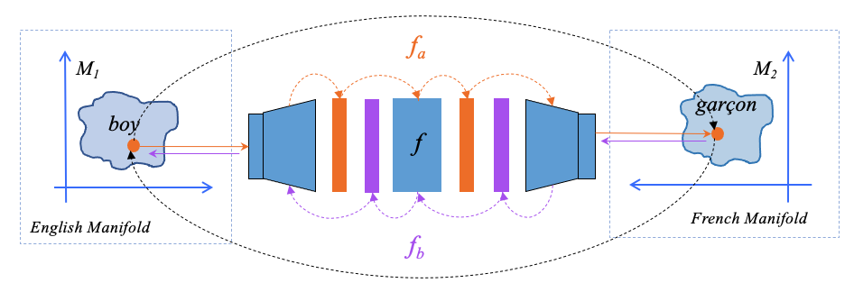
Figure 1: Mapping vector spaces with Bi-Directional Manifold Alignment (BDMA). $f$ is the feedforward network. $f_{a}$ and $f_{b}$ are represent the forward and backward direction of flow through the network. In a shared BDMA network, the blue components represent network fully connected layers, orange are activation layers during forward network flow while purple represents activation layers in reverse flow. During reverse flow from output to input, the weight matrix is a transpose of weights during forward flow through the network.

2 Bi-Directional Manifold Alignment

Consider two manifolds $M^{s}\in\mathbb{R}^{n\times d}$ (source domain) and $M^{t}\in\mathbb{R}^{m\times d}$ (target domain) that are vector space representations of words. The monolingual word embeddings are pretrained from a large corpus and may be created using different methods. Let $V^{s}$ and $V^{t}$ be the respective vocabularies of the two languages. Hence $V^{s}=\{w^{s}_{1}\ ...\ w^{s}_{n}\}$ and $V^{t}=\{w^{t}_{1}\ ..\ w^{t}_{m}\}$ are words in each vocabulary of size $n$ and $m$. The distributed representations of words in each manifold are $M^{s}=\{m^{s}_{1}\ ...\ m^{s}_{n}\}$ and $M^{t}=\{m^{t}_{1}\ ...\ m^{t}_{m}\}$. We assume there is $V^{p}=\{w^{p}_{1}\ ...\ w^{p}_{c}\}$, an available dictionary or parallel corpus of words for the given source/target pair.

2.1 Bi-Directional Loss Mechanism

We achieve bi-directional alignment by learning a mapping function is optimized with a cyclic-consistency loss (CCL). In Figure 1, the mapping function $f_{a}:M^{s}\rightarrow M^{t}$ to align the manifold $M^{s}$ to $M^{t}$. We also use a backward mapping function $f_{b}:M^{t}\rightarrow M^{s}$ to align the manifold $M^{t}$ to $M^{s}$. We refer to the parameters of both $f_{a}$ and $f_{b}$ as $\theta_{f}$.

Our method is based on jointly minimizing the distance $\mathcal{D}$ between pairs of embeddings, and their mapped counterparts, from each manifold. We define our cycle consistency loss for a single training sample based on this distance function $\mathcal{D}$ as

$$\mathcal{L}_{\textrm{ccl}}^{\mathcal{D}}(i)=\mathcal{D}(f_{a}(m^{s}_{i}),m^{t}_{i})+\mathcal{D}(f_{b}(m^{t}_{i}),m^{s}_{i}).$$ (1)

Following previous work Xing et al. (2015), we include an orthogonal loss in the objective; we extend this loss function for a neural network by performing a layerwise orthogonal loss. For our full objective, we sum over all training instances and minimize over $\theta_{f}$:

$$\mathcal{L}_{\textrm{ccl}}=\min_{\theta_{f}}\sum_{i\in V^{p}}\mathcal{L}_{\textrm{ccl}}^{\mathcal{D}}(i)+\sum_{w_{j}\in\theta_{f}}w_{j}w_{j}^{T}-I$$ (2)

where $w_{j}$ are weights of layer $j$ in the network. While Euclidean distance (mean squared error: $\mathcal{D}=\mathrm{MSE}$) is a common way of computing distance in a manifold Ruder et al. (2019); Artetxe et al. (2016), cosine or relaxed cross-domain similarity local scaling (RCSLS) Joulin et al. (2018) distance functions have been shown to be effective for word and embedding alignment tasks. Our formulation works with these other computable distance functions. For example, while applying $\mathcal{D}={\textrm{MSE}}$, and for ease omitting the orthogonal loss term $\sum_{w_{j}\in\theta_{f}}w_{j}w_{j}^{T}-I$, the loss is

$$\min_{\theta_{f}}\sum_{i\in V^{p}}\left\|f_{a}(m^{s}_{i})-m^{t}_{i}\right\|^{2}_{2}+\left\|f_{b}(m^{t}_{i})-m^{s}_{i}\right\|^{2}_{2}.$$

See Appendix D for similar formulations for $\mathcal{D}=\mathrm{cosine}$, $\mathcal{D}=\mathrm{RCSLS}$, and a combined distance function $\mathcal{D}=\mathrm{cosine+RCSLS}$ (used in §3).

2.2 Forward - Reverse Network Flow

As described in §2.1, $f_{a}$ and $f_{b}$ represent the forward and reverse network flow. We represent the forward and reverse mapping with two networks that have shared or independent parameters. When the parameters are independent, two separate networks are trained simultaneously and optimized in order to learn the mapping between two languages. In Figure 1, the network parameters are shared in our model. The forward flow is shown in orange while reverse flow is depicted in purple.

Although the two networks share parameters, they cannot do so directly as the required shapes of each layer differ. In order to perform backward translation, reverse flow is enabled in the network by explicitly taking the transpose of each layer in the network (we use fully connected layers without bias vectors) making the network bi-directional or invertible. With our cycle consistency loss formulation, the model learns layers such that the transpose of the layer inverts the network.

Method	Evaluation [s $\rightarrow$ t] P@1
	En$\rightarrow$Es	Es$\rightarrow$En	En$\rightarrow$It	It$\rightarrow$En	En$\rightarrow$De	De$\rightarrow$En	En$\rightarrow$Fr	Fr$\rightarrow$En
MUSE Conneau et al. (2017)*	81.7	83.3	77.7	78.2	74.0	72.0	82.3	82.1
VECMAP Artetxe et al. (2018)	80.80	85.20	77.47	80.47	73.33	75.07	81.60	84.40
GeoMM Jawanpuria et al. (2019)	81.53	86.33	78.47	81.53	74.80	76.67	82.00	84.67
RCSLS Joulin et al. (2018)*	84.1	86.3	78.5	79.8	79.1	76.3	83.3	84.1
BLISS(R) Patra et al. (2019)*	84.3	86.2	79.3	82.4	79.1	76.6	83.9	84.7
Joint Align Wang et al. (2019)**	69.6	71.9	-	-	68.7	70.7	78.0	79.2
Cross-lingual Anchoring Ormazabal et al. (2020)**	84.2	86.5	-	-	78.1	76.9	84.9	85.0
LNMAP (LIN. AE) Mohiuddin et al. (2020)*	82.9	86.4	78.1	81.4	75.5	75.9	83.9	84.7
Linear Mapping
BDMA [C + R] (s $\rightarrow$ t)	83.13	83.26	78.60	78.60	76.13	74.73	83.73	82.86
BDMA [C + R] (t $\rightarrow$ s)	83.13	84.06	78.60	78.53	73.46	75.66	82.8	83.86
1-Hidden Layer Feedforward Network
BDMA [C + R] (s $\rightarrow$ t)	82.40	85.73	78.66	82.60	74.46	78.40	83.40	84.93
BDMA [C + R] (t $\rightarrow$ s)	81.60	86.80	78.4	82.66	73.46	74.86	79.86	84.33

Table 1: Bi-Directional Manifold Alignment (BDMA) measured with Precision @ 1 measured on filtered MUSE evaluation set (with polysemous words) for high resource languages. * represents results taken directly from the cited paper. ** represents results taken from Ormazabal et al. (2020). We consider the best results for each language pair and direction from this paper. - represents language pairs that are not part of experiments in the original paper. BLISS(R) Patra et al. (2019) is semi-supervised.

Method	Evaluation [s $\rightarrow$ t] P@1
	En$\rightarrow$Ru	Ru$\rightarrow$En	En$\rightarrow$Hi	Hi$\rightarrow$En	En$\rightarrow$Ja	Ja$\rightarrow$En	En$\rightarrow$Pt	Pt$\rightarrow$En
VECMAP Artetxe et al. (2016)	52.33	65.73	34.87	50.03	51.54	41.42	80.27	80.67
VECMAP Artetxe et al. (2018)	51.53	70.00	40.40	56.46	46.95	44.25	80.60	82.93
GeoMM Jawanpuria et al. (2019)	54.13	69.47	-	54.72	27.55	23.66	81.60	83.27
Linear Mapping
BDMA [C + R] (s $\rightarrow$ t)	55.80	68.66	36.80	54.58	53.59	38.52	80.40	84.20
BDMA [C + R] (t $\rightarrow$ s)	55.60	69.73	36.60	55.25	53.52	38.73	80.06	83.93
1-Hidden Layer Feedforward Network
BDMA [C + R] (s $\rightarrow$ t)	57.20	70.20	37.00	54.11	54.07	46.51	80.13	83.13
BDMA [C + R] (t $\rightarrow$ s)	56.93	70.06	37.00	54.38	54.28	47.07	80.06	83.93

Table 2: Bi-Directional Manifold Alignment (BDMA) measured with Precision @ 1 on default MUSE evaluation set (with polysemous words) for low-resource languages.

3 Experiments & Analysis

We experiment with the MUSE dataset Conneau et al. (2017). It consists of $110$ bilingual dictionaries with separate training and test datasets for each language pair. The pairs contain polysemous words. When it comes to training BDMA, polysemous words can provide additional context to the model being trained while handicapping other baseline models. We filter out training pairs for polysemous words (source or target). The models are trained with $5000$ unique pairs. We show two sets of experiments: (a) with a filtered evaluation set that contains $1500$ unique pairs and (b) with the original evaluation dataset. We measure the performance of BDMA on two sets of languages: the low-resource languages Russian (Ru) and Japanese (Ja), and the high-resource languages Spanish (Es), French (Fr), German (De) and Italian (It).

In each table, s is the source language while t is the target language. $\rightarrow$ indicates the direction of mapping and training language pairs used from MUSE. For reverse translation, the model is trained with the t $\rightarrow$ s dataset and evaluated on the s $\rightarrow$ t test dataset—for example, the model trained on En$\rightarrow$Ru is evaluated on Ru$\rightarrow$En. P@1 measurements highlighted in blue show the forward (training) direction in which the model is trained and its adjacent non-colored measurement uses the same model to perform reverse translation.

Method	Evaluation [s $\rightarrow$ t] P@1
	En$\rightarrow$Es	Es$\rightarrow$En	En$\rightarrow$It	It$\rightarrow$En	En$\rightarrow$De	De$\rightarrow$En	En$\rightarrow$Fr	Fr$\rightarrow$En
MUSE Conneau et al. (2017)	48.06	61.27	51.33	62.59	37.4	50.21	39.33	51.60
VECMAP Artetxe et al. (2016)	48.87	61.49	52.07	62.31	38.60	50.22	47.47	59.10
VECMAP Artetxe et al. (2018)	48.27	62.79	52.20	65.24	37.80	52.59	47.67	60.89
GeoMM Jawanpuria et al. (2019)	48.60	63.79	52.53	65.38	38.33	53.45	48.60	61.24
RCSLS Joulin et al. (2018)	49.26	64.29	53.00	66.52	38.93	53.73	47.66	59.74
Linear Mapping
BDMA [C + R] (s $\rightarrow$ t)	49.40	62.57	52.80	63.09	39.33	52.37	48.73	59.95
BDMA [C + R] (t $\rightarrow$ s)	49.33	62.78	52.46	63.31	39.00	52.01	49.06	59.38
1-Hidden Layer Feedforward Network
BDMA [C + R] (s $\rightarrow$ t)	48.90	62.28	52.06	65.02	38.46	51.86	48.86	60.67
BDMA [C + R] (t $\rightarrow$ s)	48.46	63.00	52.46	65.09	39.06	52.08	47.33	60.67

Table 3: Bi-Directional Manifold Alignment (BDMA) measured with Precision @ 1 shows the performance of different models on high-resource languages in the MUSE dataset Conneau et al. (2017) in comparison to BDMA. The test dataset contains unique pairs only.

Method	Evaluation [s $\rightarrow$ t]
	En$\rightarrow$Ru	Ru$\rightarrow$En	En$\rightarrow$Hi	Hi$\rightarrow$En	En$\rightarrow$Ja	Ja$\rightarrow$En	En$\rightarrow$Pt	Pt$\rightarrow$En
VECMAP Artetxe et al. (2016)	35.27	52.28	23.80	26.45	39.07	35.59	44.93	61.06
VECMAP Artetxe et al. (2018)	34.53	56.28	27.40	31.21	36.20	38.88	49.53	63.83
GeoMM Jawanpuria et al. (2019)	36.93	56.42	27.67	30.35	21.60	21.81	50.13	63.90
RCSLS Joulin et al. (2018)	37.73	54.85	24.80	26.80	39.40	38.80	49.06	64.53
Linear Mapping
BDMA [C + R] (s $\rightarrow$ t)	37.40	52.35	25.20	26.87	40.8	34.64	49.46	63.12
BDMA [C + R] (t $\rightarrow$ s)	36.93	52.99	24.73	27.37	40.4	35.30	49.00	63.40
1-Hidden Layer Feedforward Network
BDMA [C + R] (s $\rightarrow$ t)	37.73	52.06	25.13	27.73	40.93	37.70	49.46	63.12
BDMA [C + R] (t $\rightarrow$ s)	38.40	53.49	25.13	29.14	40.00	38.14	48.73	64.32

Table 4: Bi-Directional Manifold Alignment (BDMA) measured with Precision @ 1 on unique MUSE evaluation set (without polysemous words) for low-resource languages.

Loss	Evaluation [s $\rightarrow$ t] P@1
	En$\rightarrow$Ru	Ru$\rightarrow$En	En$\rightarrow$Ja	Ja$\rightarrow$En
Linear Mapping (s $\rightarrow$ t)
[M]	54.66	66.26	21.93	16.26
[C]	55.00	66.46	52.22	40.38
[R]	51.80	67.53	38.51	39.53
[C + R]	55.80	68.66	53.59	38.52
Linear Mapping (t $\rightarrow$ s)
[M]	53.66	65.20	21.86	16.54
[C]	54.93	66.46	52.15	40.38
[R]	52.13	67.93	38.58	39.49
[C + R]	55.60	69.73	53.52	38.73
1-Hidden Layer Feedforward Network (s $\rightarrow$ t)
[M]	51.40	63.66	20.28	12.19
[C]	55.00	65.86	52.84	40.38
[R]	52.26	68.80	49.96	47.48
[C + R]	57.20	70.20	54.07	46.51
1-Hidden Layer Feedforward Network (t $\rightarrow$ s)
[M]	49.80	64.26	17.95	18.26
[C]	54.06	66.00	53.80	40.45
[R]	52.46	68.60	49.48	47.07
[C + R]	56.93	70.06	54.28	47.07

Table 5: Precision @ 1 of BDMA with different losses. An ablation study of the impact of different loss combinations while training a model with BDMA. [M] = MSE, [C] = cosine, [R] = RCSLS and [C + R] = cosine + RCSLS loss.

Embeddings & Baselines.

We use normalized and mean-centered FastText embeddings Joulin et al. (2016), learned from language-specific Wikipedia. We train two types of translation models: (a) a linear mapping with a weight matrix $W\in\mathbb{R}^{d\times d}$ for a $d$-dimensional embedding, and (b) a $1$ hidden layer feed forward network. For baseline comparisons, we retrain VECMAP Artetxe et al. (2016, 2018), GeoMM Jawanpuria et al. (2019) and RCSLS Joulin et al. (2018). When possible, we compare with BLISS(R) Patra et al. (2019), Joint Align Wang et al. (2019), Cross-lingual Anchoring Ormazabal et al. (2020) and LNMAP Mohiuddin et al. (2020) using results previously reported for high resource languages. We train BDMA with a combination of cosine (C) and RCSLS (R) losses, and separate baseline methods for each language and translation direction pair.

3.1 Impact of Polysemy

In Table 1, we observe BDMA’s performance translating words in high resource languages. BDMA’s performance is better or equivalent in comparison to other methods. Additionally, we note that the translation model is trained with $5000$ unique pairs while Joint Align Wang et al. (2019) and cross-lingual anchoring Ormazabal et al. (2020) are trained with the full MUSE training dataset for any given language pair which is greater than $5$K. Similarly, Table 2 shows the performance of different models on low resource languages compared to BDMA. BDMA with $1$-H FFN performs better than a linear mapping with an overall increase as high as $2.82\%$ while translating Japanese to English. The exception is for Hindi, where the performance drops by $3.8$% (Hi $\rightarrow$ En). We see that the model benefits from bidirectional training when there are polysemous words in the evaluation corpus, improving the network’s ability to generalize.

3.2 Impact of Unique Vocabulary

Similar to the previous experiment, we analyze the impact of BDMA with an evaluation dataset of unique pairs for both high resource and low resource languages. In contrast to Table 1, Table 3 shows that both linear mapping and $1$-H neural network are comparable to other baselines (except RCSLS) when there are no polysemous words. Adding additional layers to the network does not provide any benefit, which is consistent with findings from Søgaard et al. (2018) and Ruder et al. (2019) that a linear mapping performs well for these language pairs. Table 4 details experiments for the same under low resource language conditions. Although BDMA performs better for En $\rightarrow$ Ru and En $\rightarrow$ Ja, Hi $\rightarrow$ En continues to perform poorly. In contrast, its performance is comparable for Portuguese where the reduction is $1.13$% (En $\rightarrow$ Pt) only.

Therefore, the $2$ main benefits of BDMA are: (a) it creates a single bidirectional word translation model while keeping the performance of the model comparable to baseline, and (b) the $1$-H FFN is a single network in comparison to LNMAP (which has $3$), while Linear BDMA has the same number of parameters as all other methods in Table 1 and 2.

3.3 Importance of Training Direction

If the filtered training pairs do not contain polysemous words, why is the training direction important? This is because when the model is trained for a number of epochs, its optimal savepoint is chosen based on the forward translation performance for the given language pair direction. As seen in Table 2 and 4, the direction chosen to start model training can have an impact of forward and reverse translation performance. For example, the model training with Ru $\rightarrow$ En performs better than En $\rightarrow$ Ru.

Ablation Study.

In Table 5, we assess the impact of using (combinations of) MSE, cosine and RCSLS distance functions $\mathcal{D}$. A combined cosine and RCSLS loss ([C + R]) performs the best and provides consistent forward ($s\leftarrow t$) and reverse translation ($t\leftarrow s$) performance (within $0.5\%$).

4 Related Work

Over the years, many supervised methods have been proposed. Irvine and Callison-Burch (2013) learn a binary classifier for a language pair that predicts if a given word pair is a translation of each other or not. Artetxe et al. (2016) implement Procrustes alignment while normalizing and mean centering word embeddings. Xing et al. (2015) add an orthogonal loss while aligning manifolds. In Artetxe et al. (2018), additional pre- and post-processing steps are provided. Conneau et al. (2017) propose a new retrieval method called cross-domain similarity local scaling (CSLS) in order to reduce the “hubness” problem. Joulin et al. (2018) convert CSLS into a loss objective in order to optimize the translation matrix. An important challenge with linear mapping is that it assumes that source and target languages have a similar manifold structure; Søgaard et al. (2018) show this assumption is not true for many language pairs. Nakashole and Flauger (2018) show that transformations need to be non-linear and are dependent on the word’s local neighborhood. Instead of learning a mapping between languages separately, Wang et al. (2019) jointly learn the monolingual and cross-lingual embeddings for the given language pair. Ormazabal et al. (2020) extend skip-gram to project source embeddings into a fixed target space and using them as anchors to iteratively learn the mapping.

Cyclic Loss for Reverse Translation. Xu et al. (2018) perform unsupervised word alignment using the cycle consistency loss while computing the sinkhorn distance between a forward and reverse translation network. Mohiuddin and Joty (2019) train a dual autoencoder-discriminator architecture and use a cyclic loss to train a bi-directional model. LNMAP Mohiuddin et al. (2020) extends the autoencoder architecture with a 2 layer mapping to learn a non-isomorphic mapping between languages. Our work differs as we reduce the number of parameters in the model (as it contains the mapping only) while training an invertible network that can perform both forward and back translation.

5 Conclusion

We show how a non-linear mapping (invertible neural network) can be trained with a cyclic consistency loss, showing that a common isomorphic assumption is not strictly necessary Søgaard et al. (2018). The network trained has fewer parameters in comparison to Mohiuddin et al. (2020) while providing equivalent or improved performance on the low-resource word translation task.

Appendix

In the following sections, we provide information about hyperparameter values for each network architecture, statistics about the dataset and results from additional experiments. The experiments are conducted on a NVIDIA K20 GPU with $\approx 4$GB of RAM and NVIDIA V100 GPUs with $16$GB of RAM. Each model is trained on a single GPU. Linear models can be trained on K20s and the larger $1$-H-FFN are optimized on V100s.

Appendix A Hyperparameters

Following are the hyper-parameters used in our experiments:

Hyper-parameter	Value
batch size	$128$
lr_decay	$0.98$
lr_shrink	$0.5$
map_beta	$0.001$
max_vocab	$200000$

Table A1: Hyperparameters for BDMA experiments.

As seen in table A1, the maximum vocabulary (max_vocab) size is $200K$. The vocabulary is selected by taking $200K$ words that have the highest frequency. map_beta is the parameter that controls the contribution of the orthogonal loss to the overall loss function. The network is trained with an Adam optimizer Kingma and Ba (2014) having a learning rate of $0.0005$. The word embeddings are preprocessed i.e. they are normalized and centered. The $1$ hidden layer feedforward network used to perform alignment has a hidden layer size of $4096$. The activation function of the hidden layer is tanh.

Appendix B CCL Correlation with Linear Mapping

As observed in equation 2.1, a linear relationship between source and target language embeddings can be learned by minimizing the squared loss between them. Although, in practice, an additional orthogonal constraint $\mathcal{L}_{ortho}=WW^{T}-I$ is added Xing et al. (2015) as shown in the equation below:

$$\mathcal{L}_{\textrm{mse}}=\sum_{i\in V^{p}}\overbrace{\left\|f_{a}(m^{s}_{i})-m^{t}_{i}\right\|^{2}_{2}}^{\mathcal{L}_{\textrm{mse}}^{i}}+(WW^{T}-I),$$ (3)

Minimizing $\mathcal{L}_{ortho}$ makes the linear mapping implicitly bidirectional able to map words from the target to source language. In comparison, $\mathcal{L}_{ccl}$ in equation 1 trains a non-linear neural network or linear mapping to be explicitly bidirectional. Thus $\mathcal{L}_{ccl}$ can be considered as an extension of $\mathcal{L}_{ortho}$.

Target Language	Train	Test
French	$10872$	$2943$
German	$14677$	$3660$
Italian	$9657$	$2585$
Spanish	$11977$	$2975$
Russian	$10887$	$2447$
Hindi	$8704$	$2032$
Japanese	$7135$	$1799$
Portuguese	$11185$	$2827$

Table A2: MUSE Dictionary Size. The table shows the target language, the number of pairs in the training and pairs present in the test dictionary where the source language is English.

Source Language	Train	Test
French	$8270$	$2342$
German	$10866$	$2827$
Italian	$7364$	$2102$
Spanish	$8667$	$2416$
Russian	$7452$	$2069$
Hindi	$8001$	$1963$
Japanese	$6819$	$1952$
Portuguese	$7582$	$2148$

Table A3: The table shows the source language, the number of pairs in the training and pairs present in the test dictionary where the target language is English.

Appendix C Dataset

MUSE Conneau et al. (2017). As described in §3, the dataset has $110$ bilingual dictionaries and contains pairs with English being the source or target language. Additionally, Non-English language pairs are available for European languages that includes German, Spanish, French, Italian and Portuguese. Each bilingual dataset has a vocabulary of $5000$ unique source language words to train the translation model and $1500$ unique words to evaluate them. Because the pairs are not unique and contain polysemous source words (the target word is always unique), the overall size of training and test dictionaries is greater than $5000$ and $1500$.

Tables A2 and A3 show the dataset size from the original MUSE dataset. The tables show that samples for different language pairs contain polysemous words that expand dataset size by $36.8$% to $123.7$% in comparison to BDMA (in table 2, 4 and 1) that is trained with $5000$ unique pairs only.

Appendix D Additional Loss

In §2.1, we showcased how MSE is adapted for $\mathcal{L}_{\textrm{ccl}}$. Similarly, cosine and Relaxed CSLS loss can be modified for BDMA too. In an adapted version of cosine loss, we minimize the following:

$$\min_{\theta_{f}}\sum_{i\in V^{p}}(1-|f_{a}(m^{s}_{i})\cdot m^{t}_{i}|)+(1-|f_{b}(m^{t}_{i})\cdot m^{s}_{i}|)$$

In order to modify RCSLS Joulin et al. (2018), we first take look at CSLS Conneau et al. (2017) criteria for retrieval:

$$\text{CSLS}(m^{s}_{i},m^{t}_{i})=-2\text{cos}(m^{s}_{i},m^{t}_{i})+\frac{1}{\text{k}}\sum_{m^{t}_{j}\in\mathcal{N}^{t}(\mathcal{W}\cdot m^{s}_{i})}\text{cos}(\mathcal{W}m^{s}_{i},m^{t}_{j})+\frac{1}{\text{k}}\sum_{m^{s}_{j}\in\mathcal{N}^{s}(\mathcal{W}^{\mathcal{T}}\cdot m^{t}_{i})}\text{cos}(m^{s}_{j},\mathcal{W}^{\mathcal{T}}m^{t}_{i}))$$ (4)

where $\mathcal{N}^{s}(x)$ is the neighborhood of $x$ in the source manifold and $\mathcal{N}^{t}(y)$ is the same in the target, k is the number of nearest neighbors and $\mathcal{W}$ is assumed to be orthogonal. Joulin et al. (2018) relax the cosine criteria in RCSLS i.e. $\text{cos}(\mathcal{W}m^{s}_{i},m^{t}_{i})={m^{s}_{i}}^{\mathcal{T}}\mathcal{W}^{\mathcal{T}}m^{t}_{i}$. Hence RCSLS becomes:

$$\text{RCSLS}(m^{s}_{i},m^{t}_{i})=-2{m^{s}_{i}}^{\mathcal{T}}\mathcal{W}^{\mathcal{T}}m^{t}_{i}+\frac{1}{\text{k}}\sum_{m^{t}_{j}\in\mathcal{N}^{t}(\mathcal{W}\cdot m^{s}_{i})}{m^{s}_{i}}^{\mathcal{T}}\mathcal{W}^{\mathcal{T}}m^{t}_{j}+\frac{1}{\text{k}}\sum_{m^{s}_{j}\in\mathcal{N}^{s}(\mathcal{W}^{\mathcal{T}}\cdot m^{t}_{i})}{m^{s}_{j}}^{\mathcal{T}}\mathcal{W}^{\mathcal{T}}m^{t}_{i}$$ (5)

In BDMA, we replace the orthogonal matrix $\mathcal{W}$ with a mapping that is either linear or non-linear (neural network). RCSLS changes to:

$$\text{RCSLS}(m^{s}_{i},m^{t}_{i})=-2f_{a}(m^{s}_{i})m^{t}_{i}+\frac{1}{\text{k}}\sum_{m^{t}_{j}\in\mathcal{N}^{t}(f_{a}(m^{s}_{i}))}f_{a}(m^{s}_{i})m^{t}_{j}+\frac{1}{\text{k}}\sum_{m^{s}_{j}\in\mathcal{N}^{s}(f_{b}m^{t}_{i})}m^{s}_{j}f_{b}(m^{t}_{i})$$ (6)

In equation 6, $f_{a}$ and $f_{b}$ are the forward and reverse flow projections of $m^{s}_{i}$ and $m^{t}_{i}$ respectively.

References

- Artetxe et al. (2016) Mikel Artetxe, Gorka Labaka, and Eneko Agirre. 2016. Learning principled bilingual mappings of word embeddings while preserving monolingual invariance. In Proceedings of the 2016 Conference on Empirical Methods in Natural Language Processing, pages 2289–2294.
- Artetxe et al. (2018) Mikel Artetxe, Gorka Labaka, and Eneko Agirre. 2018. Generalizing and improving bilingual word embedding mappings with a multi-step framework of linear transformations. In Proceedings of the Thirty-Second AAAI Conference on Artificial Intelligence (AAAI-18).
- Conneau et al. (2017) Alexis Conneau, Guillaume Lample, Marc’Aurelio Ranzato, Ludovic Denoyer, and Hervé Jégou. 2017. Word translation without parallel data. arXiv preprint arXiv:1710.04087.
- Irvine and Callison-Burch (2013) Ann Irvine and Chris Callison-Burch. 2013. Supervised bilingual lexicon induction with multiple monolingual signals. In Proceedings of the 2013 Conference of the North American Chapter of the Association for Computational Linguistics: Human Language Technologies, pages 518–523, Atlanta, Georgia. Association for Computational Linguistics.
- Jawanpuria et al. (2019) Pratik Jawanpuria, Arjun Balgovind, Anoop Kunchukuttan, and Bamdev Mishra. 2019. Learning multilingual word embeddings in latent metric space: a geometric approach. Transactions of the Association for Computational Linguistics, 7:107–120.
- Joulin et al. (2018) Armand Joulin, Piotr Bojanowski, Tomas Mikolov, Hervé Jégou, and Edouard Grave. 2018. Loss in translation: Learning bilingual word mapping with a retrieval criterion. arXiv preprint arXiv:1804.07745.
- Joulin et al. (2016) Armand Joulin, Edouard Grave, Piotr Bojanowski, Matthijs Douze, Hérve Jégou, and Tomas Mikolov. 2016. Fasttext.zip: Compressing text classification models. arXiv preprint arXiv:1612.03651.
- Kingma and Ba (2014) Diederik P Kingma and Jimmy Ba. 2014. Adam: A method for stochastic optimization. arXiv preprint arXiv:1412.6980.
- Mohiuddin et al. (2020) Tasnim Mohiuddin, M Saiful Bari, and Shafiq Joty. 2020. Lnmap: Departures from isomorphic assumption in bilingual lexicon induction through non-linear mapping in latent space. arXiv preprint arXiv:2004.13889.
- Mohiuddin and Joty (2019) Tasnim Mohiuddin and Shafiq Joty. 2019. Revisiting adversarial autoencoder for unsupervised word translation with cycle consistency and improved training. arXiv preprint arXiv:1904.04116.
- Nakashole and Flauger (2018) Ndapa Nakashole and Raphael Flauger. 2018. Characterizing departures from linearity in word translation. arXiv preprint arXiv:1806.04508.
- Ormazabal et al. (2020) Aitor Ormazabal, Mikel Artetxe, Aitor Soroa, Gorka Labaka, and Eneko Agirre. 2020. Beyond offline mapping: Learning cross lingual word embeddings through context anchoring. arXiv preprint arXiv:2012.15715.
- Patra et al. (2019) Barun Patra, Joel Ruben Antony Moniz, Sarthak Garg, Matthew R Gormley, and Graham Neubig. 2019. Bilingual lexicon induction with semi-supervision in non-isometric embedding spaces. arXiv preprint arXiv:1908.06625.
- Ruder et al. (2019) Sebastian Ruder, Ivan Vulić, and Anders Søgaard. 2019. A survey of cross-lingual word embedding models. Journal of Artificial Intelligence Research, 65:569–631.
- Sahin et al. (2017) Cem Safak Sahin, Rajmonda S Caceres, Brandon Oselio, and William M Campbell. 2017. Consistent alignment of word embedding models. arXiv preprint arXiv:1702.07680.
- Søgaard et al. (2018) Anders Søgaard, Sebastian Ruder, and Ivan Vulić. 2018. On the limitations of unsupervised bilingual dictionary induction. arXiv preprint arXiv:1805.03620.
- Wang et al. (2019) Zirui Wang, Jiateng Xie, Ruochen Xu, Yiming Yang, Graham Neubig, and Jaime Carbonell. 2019. Cross-lingual alignment vs joint training: A comparative study and a simple unified framework. arXiv preprint arXiv:1910.04708.
- Xing et al. (2015) Chao Xing, Dong Wang, Chao Liu, and Yiye Lin. 2015. Normalized word embedding and orthogonal transform for bilingual word translation. In Proceedings of the 2015 Conference of the North American Chapter of the Association for Computational Linguistics: Human Language Technologies, pages 1006–1011.
- Xu et al. (2018) Ruochen Xu, Yiming Yang, Naoki Otani, and Yuexin Wu. 2018. Unsupervised cross-lingual transfer of word embedding spaces. In Proceedings of the 2018 Conference on Empirical Methods in Natural Language Processing, pages 2465–2474, Brussels, Belgium. Association for Computational Linguistics.
- Zhu et al. (2017) Jun-Yan Zhu, Taesung Park, Phillip Isola, and Alexei A Efros. 2017. Unpaired image-to-image translation using cycle-consistent adversarial networks. In Proceedings of the IEEE international conference on computer vision, pages 2223–2232.