Adaptive Capped Least Squares

Abstract

This paper proposes the capped least squares regression with an adaptive resistance parameter, hence the name, adaptive capped least squares regression. The key observation is, by taking the resistant parameter to be data dependent, the proposed estimator achieves full asymptotic efficiency without losing the resistance property: it achieves the maximum breakdown point asymptotically. Computationally, we formulate the proposed regression problem as a quadratic mixed integer programming problem, which becomes computationally expensive when the sample size gets large. The data-dependent resistant parameter, however, makes the loss function more convex-like for larger-scale problems. This makes a fast randomly initialized gradient descent algorithm possible for global optimization. Numerical examples indicate the superiority of the proposed estimator compared with classical methods. Three data applications to cancer cell lines, stationary background recovery in video surveillance, and blind image inpainting showcase its broad applicability.

Keywords: Breakdown point, capped least squares, data-dependent, efficiency, localized empirical process, $M$-estimator, resistance.

1 Introduction

Suppose we collect data points $\{(x_{i},y_{i})\}_{i=1}^{n}$ that follow a linear model

$$y_{i}=x_{i}^{\mathrm{\scriptscriptstyle T}}\beta^{*}+\epsilon_{i},\ \ i=1,\ldots,n,$$

where $y_{i}$ is a univariate response, $x_{i}$ is a $d$-dimensional predictor, $\beta^{*}$ is the regression coefficient vector, and $\epsilon_{i}$ is a random error. A standard approach for estimating $\beta^{*}$ is to solve the empirical risk minimization problem of the form

$$\widehat{\beta}\in\mathop{\mathrm{argmin}}_{\beta\in\mathbb{R}^{d}}\frac{1}{n}\sum_{i=1}^{n}f(\beta;x_{i},y_{i}),$$

where $f$ is a risk or loss function. When data are collected without contamination, the risk function $f$ is often taken as $f(\beta;x_{i},y_{i}):=\ell(y_{i}-x_{i}^{\mathrm{\scriptscriptstyle T}}\beta)=(y_{i}-x_{i}^{\mathrm{\scriptscriptstyle T}}\beta)^{2}/2$. The resulting estimator $\widehat{\beta}$ is known as the ordinary least squares (OLS) estimator, which is also the maximum likelihood estimator when the errors $\epsilon_{i}$ follow independent and identical normal distributions. Albeit having desirable statistical and computational properties, the ordinary least squares estimator is highly sensitive to outliers in both the feature and the response space.

Since the seminal work of Huber (1964), many authors have proposed robust regression methods by replacing the square loss by some loss that grows slowly at tails. For example, the Huber loss exhibits a linear growth while away from zero. Although it protects against outlying $y_{i}$, it is not robust to outliers in the feature space: one single outlier in the feature space can have arbitrary large effect on the estimate. To characterize this phenomenon, Hampel (1971) introduced the notion of breakdown point, which is defined as the smallest percentage of contaminated data that can cause the estimator to take on arbitrarily large aberrant values. Because robustness can be somewhat a broad concept, we prefer to call an estimator with high breakdown point a resistant estimator. Rousseeuw (1984) proposed the least median of squares (LMS) estimator and the least trimmed squares (LTS) estimator, which were among the first equivariant regression estimators that can attain asymptotic maximum breakdown point of $1/2$. The LMS estimator, however, only has a cubic rate of convergence and thus has zero asymptotic efficiency. The LTS estimator is asymptotically normal but has a low efficiency of $7\%$ under the normal errors (Maronna et al., 2019). Other resistant regression estimators include the S-estimator (Rousseeuw and Yohai, 1984), the $\tau$-estimator (Yohai and Zamar, 1988), the MM-estimator (Yohai, 1987), and the rank-based estimator (Wang et al., 2020). Maronna et al. (2019) have argued that the redescending $M$-estimators, such as the Tukey’s biweight $M$-estimator, achieve better balance between resistance and efficiency.

For most resistant $M$-estimators, there is often a tuning constant $\tau$, which we refer to as the resistance parameter, governing the tradeoff between resistance and efficiency. A common practice is to pick the resistance parameter based on the $95\%$ asymptotic efficiency rule (Western, 1995) so that resistance can be introduced at a manageable cost of efficiency. Despite being resistant, such an approach makes resulting estimator biased when error distributions are asymmetric (Fan et al., 2017; Sun et al., 2020). Moreover, a fixed-$\tau$ loss is asymptotically different from that derived from the likelihood principal, so that the resulting robust estimator is less efficient. Several authors have worked on improving the efficiency of an initial resistant estimator using multi-stage procedures. For example, Gervini and Yohai (2002) proposed a fully asymptotically efficient multi-stage estimator with high breakdown point: the later stages use a sequence of reweighted least squares to improve the efficiency. Bondell and Stefanski (2013) proposed an empirical-likelihood framework that down-weights outlying observations by measuring the divergence between the empirical likelihood and the normal error distribution. Both work assumes symmetric errors.

Given all the aforementioned works, it seems that efficiency and resistance can only be achieved simultaneously via multi-stage procedures. A natural question that arises is as follows: Is there a simple, one-stage estimator, without estimating any empirical distribution, that can achieve full asymptotic efficiency and maximum breakdown point? This paper gives a positive answer by proposing such a one-stage estimator. Unlike most of the literature which only considers symmetric errors with unimodal densities, we accommodate the practice where errors can be asymmetric, and characterize the tradeoff between the statistical accuracy (bias), asymptotic efficiency and robustness. The key observation is that the robustification parameter $\tau=\tau(n)$ should grow as the sample size grows, in which case the estimation bias diminishes asymptotically. From the statistical efficiency perspective, the loss function approaches to that derived from the likelihood principal under normals as the resistance parameter grows to infinity in the asymptotic limit, and thus the resulting estimator can be fully asymptotically efficient. Theoretically, we prove its asymptotic properties under mild moment conditions with increasing dimensions. Counterintuitively, by taking $\tau=\tau(n)$ to be data-dependent, the ensuing estimator maintains the robustness property, that is, it achieves the maximum high breakdown point of $1/2$ asymptotically.

Computationally, we formulate the corresponding optimization program as a mixed quadratic integer programming (MIP) problem which can be readily solved by CPLEX. However, solving MIP for the global optimum is NP-hard and thus computationally intractable for large scale problems. By allowing the resistance parameter to grow with the sample size, the problem becomes more convex-like as $n\rightarrow\infty$, and thus become easier computationally when the sample size increases. Indeed, since the empirical loss function has a growing quadratic region, first-order algorithms will converge as long as the starting point is not in the flat region. This motivates us to propose a randomly initialized gradient descent algorithm, which is able to find the global optimum with high probability. An R package that implements our algorithm can be found at https://github.com/rruimao/ACLS.

The rest of this paper proceeds as follows. In Section 2, we introduce the adaptive capped least squares regression and prove its resistance property. Section 3 is devoted to asymptotic properties where we show the proposed estimator achieves full asymptotic efficiency. Section 4 presents algorithms. Simulation studies and real data applications are provided in Sections 5 and 6 to support our method and theory. We close this paper with a discussion in Section 7.

Notation We summarize here the notation that will be used throughout the paper. For any vector $\mathrm{u}=(\mathrm{u}_{1},\ldots,\mathrm{u}_{d})^{\mathrm{\scriptscriptstyle T}}\in\mathbb{R}^{d}$ and $q\geq 1$, $\|\mathrm{u}\|_{q}=\big{(}\sum_{j=1}^{d}|\mathrm{u}_{j}|^{q}\big{)}^{1/q}$ is the $\ell_{q}$ norm. For any vectors $\mathrm{u},\mathrm{v}\in\mathbb{R}^{d}$, we write $\langle\mathrm{u},\mathrm{v}\rangle=\mathrm{u}^{\mathrm{\scriptscriptstyle T}}\mathrm{v}$. We use $C$ to denote a generic constant which may change from line to line. For two sequences of real numbers $\{a_{n}\}_{n\geq 1}$ and $\{b_{n}\}_{n\geq 1}$, $a_{n}\lesssim b_{n}$ denotes $a_{n}\leq Cb_{n}$ for some constant $C>0$, $a_{n}\gtrsim b_{n}$ if $b_{n}\lesssim a_{n}$, and $a_{n}\sim b_{n}$ indicates that $a_{n}\lesssim b_{n}$ and $b_{n}\lesssim a_{n}$. If $A$ is an $m\times n$ matrix, we use $\|A\|_{q}$ to denote its $\ell_{q}$ operator norm, defined by $\|A\|_{q}=\max_{\mathrm{u}\in\mathbb{R}^{n}}\|A\mathrm{u}\|_{q}/\|\mathrm{u}\|_{q}$.

2 Methodology

We start with definitions of the capped least squares loss and the resistance parameter.

Definition 2.1 (Capped Least Squares, CLS).

The capped least squares loss $\ell_{\tau}(\cdot)$ is defined as

$$\ell_{\tau}(x)=\begin{cases}x^{2}/2,&\textnormal{if}\ |x|\leq\tau;\\ \tau^{2}/2,&\textnormal{if}\ |x|>\tau,\end{cases}$$

where $\tau=\tau(n)>0$ is referred to as the resistance parameter.

The loss $\ell_{\tau}(\cdot)$ is quadratic for small values of $x$ and stays flat when $x$ exceeds $\tau$ in magnitude. The parameter $\tau$ therefore controls the blending of the quadratic and flat regions, and the flat region brings resistance. Define the empirical loss function $\mathcal{L}_{n,\tau}(\beta)=n^{-1}\sum_{i=1}^{n}\ell_{\tau}(y_{i}-x_{i}^{\mathrm{\scriptscriptstyle T}}\beta)$. The adaptive capped least squares estimator is then defined as

$$\widehat{\beta}_{\tau}\in\mathop{\mathrm{argmin}}_{\beta\in\mathbb{R}^{d}}\mathcal{L}_{n,\tau}(\beta)=\mathop{\mathrm{argmin}}_{\beta\in\mathbb{R}^{d}}\left\{\frac{1}{n}\sum_{i=1}^{n}\ell_{\tau}(y_{i}-x_{i}^{\mathrm{\scriptscriptstyle T}}\beta)\right\}.$$ (2.1)

With a growing resistance parameter $\tau=\tau(n)$, the empirical loss $\mathcal{L}_{n,\tau}(\beta)$ approaches the least squares loss function, so that the ensuing estimator is asymptotically unbiased and efficient. Perhaps surprisingly, this does not cause any loss of resistance. We will use the term, adaptive capped least squares (ACLS), to emphasize the fact that $\tau=\tau(n)$ should be data-dependent. This distinguishes our framework from classical redescending-type estimators.

Comparing with the ordinary least squares estimator, outliers are completely removed in the estimation procedure (2.1) which leads to resistance. To see this, we first fix $\tau$ and write $\psi_{\tau}(x)=x1(|x|\leq\tau),$ which can be thought as the first order derivative of $\ell_{\tau}(x)$, except at the point of $\tau$ and $-\tau$. Heuristically, $\widehat{\beta}_{\tau}$ solves the estimating equations

$$\frac{1}{n}\sum_{i=1}^{n}\psi_{\tau}(y_{i}-x_{i}^{\mathrm{\scriptscriptstyle T}}\beta)x_{i}=0.$$

Note that $\psi_{\tau}(r_{i})=0$ if the $i$-th residual $r_{i}=y_{i}-x_{i}^{\mathrm{\scriptscriptstyle T}}\beta$ exceeds $\tau$ in magnitude, which corresponds to a “bad” fit possibly due to an outlying observation for the $i$-th individual. As a result, this sample does not contribute to the above estimating equations. This implies that the capped least squares estimator could be more robust than the Huber estimator (Huber, 1964). Comparing with other redescending-type losses such as the Tukey’s biweight loss, the CLS estimator is more efficient. This is because the CLS loss is exactly quadratic in the center while, for example, the Tukey’s biweight loss is not. Figure 1 shows the relative efficiency of the Tukey’s biweight estimator over the CLS estimator over a sequence of same tuning parameters $\tau$. We shall mention that the CLS estimator is also referred to as the trimmed mean estimator under location models (Huber, 1964).

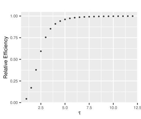
Figure 1: Relative efficiency of the Tukey’s biweight estimator vs the CLS estimator.

While $\tau$ serves as a capping parameter that encourages resistance, at first sight it seems that $\widehat{\beta}_{\tau}$ will lose resistance when $\tau=\tau(n)$ tends to infinity with $n$. Perhaps surprisingly, at least to us, we will show in what follows: the resistance property is preserved as long as $\tau=\tau(n)$ is fixed for every $n$. Denote the collected $n$ data vectors by $\mathcal{Z}=\{z_{1},\ldots,z_{n}\}$, where $z_{i}=(x_{i},y_{i})$. For any estimator $\widehat{\beta}$, as a function of $\mathcal{Z}$, the finite-sample breakdown point $\varepsilon^{*}(\widehat{\beta},\mathcal{Z})$ of $\widehat{\beta}$ (Donoho and Huber, 1983; Hampel, 1971) is defined as

$$\varepsilon^{*}(\widehat{\beta},\mathcal{Z})=\frac{1}{n}\min\Bigg{\{}m:\sup_{\widetilde{\mathcal{Z}}\in\mathcal{P}_{m}(\mathcal{Z})}\big{\|}\beta(\widetilde{\mathcal{Z}})\big{\|}_{2}=\infty\Bigg{\}},$$

where $\mathcal{P}_{m}(\mathcal{Z})=\big{\{}\widetilde{\mathcal{Z}}:\,\widetilde{z}_{i}\neq z_{i},\,i\in\mathcal{I}~{}\textnormal{s.t.}~{}|\mathcal{I}|\leq m\big{\}}$. Denote by $\mathcal{G}$ the set of uncontaminated/clean samples. The following result is on the breakdown point of the Huber estimator, taken from Maronna et al. (2019).

Proposition 2.2.

The Huber estimator has breakdown point at most $1/n$.

The above proposition demonstrates that the Huber estimator, and thus the adaptive Huber estimator, is not robust to outliers in the feature space. Our first main result is on the high breakdown point of the proposed ACLS estimator, under the general position assumption (Mili et al., 1996).

Assumption 1 (General Position).

We assume the data are in general position, that is, any $d$ of them give a unique determination of $\beta$.

Theorem 2.3 (High Breakdown Point).

Assume Assumption 1 and let $c_{r}=\sum_{i\in\mathcal{G}}\epsilon_{i}^{2}/(2|\mathcal{G}|)$. Then, the adaptive capped least squares estimator has breakdown point of at least

$$\frac{1}{n}\left(\frac{n(1-2c_{r}/\tau^{2})-d+1}{2(1-c_{r}/\tau^{2})}\right)\rightarrow\frac{1}{n}\left\lfloor\frac{n-d+2}{2}\right\rfloor~{}\textnormal{as}~{}\tau^{2}/c_{r}\rightarrow\infty.$$

Note that the adaptive capped least squares regression estimator is regression equivariant (Rousseeuw and Leroy, 1987), that is,

$$\widehat{\beta}_{\tau}\big{(}\{x_{i},y_{i}+x_{i}v),i=1,\ldots n\}\big{)}=\widehat{\beta}_{\tau}\big{(}\{x_{i},y_{i}),i=1,\ldots n\}\big{)}+v$$

for any $v\in\mathbb{R}^{d}$. The maximum breakdown point for regression equivariant estimator is $\left\lfloor(n-d+2)/2\right\rfloor/n$ (Müller, 1995; Mizera and Müller, 2002). Therefore, provided that $\tau^{2}/c_{r}\rightarrow\infty$, the adaptive capped least squares regression estimator achieves the maximum breakdown point asymptotically.

A common practice is to determine $\tau$ by the $95\%$ asymptotic efficiency rule (Maronna et al., 2019) to introduce resistance at the cost of efficiency. Yet our result suggests that, by letting $\tau=\tau(n)$ to be data-dependent and diverging, high breakdown point can be preserved. At the same time, full asymptotic efficiency is achieved as the CLS loss is exactly quadratic in an increasing region (with $n$) around the origin. This is somewhat counter-intuitive at first glance. A careful examination, however, reveals that these two properties do not necessarily contradict each other. This is because the breakdown point is a finite-sample property while the statistical efficiency is an asymptotic notion.

To illustrate the intuition, let us consider estimating the mean of a random variable. Suppose the uncontaminated data $\{y_{i}\}_{i=1}^{n}$ follow the local model

$$y_{i}=\mu+\epsilon_{i},~{}i=1,\ldots,n,$$

while we only observe the contaminated versions $\widetilde{y}_{i}=y_{i}+\gamma_{i}$ with $\gamma_{i}$ denoting a mean shift parameter to indicate the deterministic contamination. The breakdown point of a procedure can be roughly understood as how many arbitrary $\gamma_{i}$’s the procedure can tolerate before it produces arbitrarily large estimates. For any fixed $n$ and $\tau(n)<\infty$, the procedure $\mathop{\mathrm{argmin}}_{\mu}(1/n)\sum_{i=1}^{n}\ell_{\tau}(\widetilde{y}_{i}-\mu)$ achieves high breakdown point by eliminating the effects of arbitrarily large $\gamma_{i}$’s when $|\widetilde{y}_{i}-\mu|>\tau$. In other words, the breakdown point property does not depend on the actual value of $\tau$ as long as it is finite for every $n$. On the other hand, a data-dependent and diverging $\tau$ brings full asymptotic efficiency. We prove this rigorously in the next section.

Finally, we point out that, in the processing of finishing this manuscript, the authors were pointed out a previous paper by He et al. (2000) showed that weighted $t$-type regression estimators of a can have high breakdown points and are efficient for certain heteroscedastic $t$-models due to being maximum likelihood estimators. Simpson (1987) showed full efficiency and resistance for minimum Hellinger distance estimator but only at a target model like a Poisson model for count data. These work showed the promise of developing a single-stage fully efficient and highly resistant estimator in the general case, as provided by our paper.

3 Asymptotic Properties

This section establishes the asymptotic properties for the proposed robust estimator. For any prespecified $\tau>0$, $\widehat{\beta}_{\tau}$ is an $M$-estimator of

$$\beta_{\tau}^{*}=\mathop{\mathrm{argmin}}_{\beta\in\mathbb{R}^{d}}\mathcal{L}_{\tau}(\beta)~{}\mbox{ with }~{}\mathcal{L}_{\tau}(\beta):=\frac{1}{n}\sum_{i=1}^{n}\mathbb{E}\ell_{\tau}(y_{i}-x_{i}^{\mathrm{\scriptscriptstyle T}}\beta).$$

We call $\beta_{\tau}^{*}$ the capped least squares regression coefficient, which is not necessarily equal to $\beta^{*}$ unless the error distributions are symmetric. By setting $\tau=\infty$, we have $\beta^{*}_{\infty}=\beta^{*}$ as long as $\mathbb{E}[\epsilon_{i}|x_{i}]=0$. Throughout the paper, we assume that the capped least squares regression coefficient approaches $\beta^{*}$ as $\tau\rightarrow\infty$, that is, $\|\beta_{\tau}^{*}-\beta^{*}\|_{2}\rightarrow 0$ as $\tau\rightarrow\infty$. To prove consistency, we impose the following assumption, which essentially assumes that the population global optimum is unique.

Assumption 2 (Separability).

For every $\varepsilon>0$, $\beta\to\mathcal{L}_{\tau}(\beta)$ with $\tau>0$ sufficiently large satisfies

$$\inf_{\beta:\|\beta-\beta_{\tau}^{*}\|_{2}\geq\varepsilon}\mathcal{L}_{\tau}(\beta)>\mathcal{L}_{\tau}(\beta_{\tau}^{*}).$$

Theorem 3.1 (Consistency).

Suppose Assumption 2 holds. Provided that the triplet $(d,n,\tau)$ satisfies $\tau^{4}d/n\rightarrow 0$ as $n\to\infty$, we have $\widehat{\beta}_{\tau}\overset{\mathbb{P}}{\to}\beta^{*}_{\tau}$. In addition, if $\tau\rightarrow\infty$, then $\widehat{\beta}_{\tau}\overset{\mathbb{P}}{\to}\beta^{*}.$

The above theorem shows that as long as $\tau$ does not grow too fast, the capped least squares estimator $\widehat{\beta}_{\tau}$ is consistent. Technically, if we take the parameter space to be a compact subset of $\mathbb{R}^{d}$, then the scaling condition in Theorem 3.1 can be relaxed to $\tau=o(\sqrt{n})$. To obtain the convergence rate and the asymptotic normality, we need the following anti-concentration type property for random errors.

Assumption 3 (Anti-concentration).

There exist positive constants $L_{0}$, $\eta$ and $\tau_{0}$ such that for any $\Delta\in[0,\tau/2]$ and $\tau\geq\tau_{0}$,

$$\max_{1\leq i\leq n}\mathbb{E}\left\{|\epsilon_{i}|^{4+\eta}1(\tau-\Delta\leq|\epsilon_{i}|\leq\tau+\Delta)\right\}\leq\frac{L_{0}\Delta}{\tau}.$$

Assumption 3 is an anti-concentration-type condition on the distributions of $\epsilon_{i}$. It is satisfied if the density of $\epsilon_{i}$ decays sufficiently fast. For example, assume $\epsilon_{i}$’s are independent and identically distributed, and denote by $p(\cdot)$ the density function of $|\epsilon_{i}|$. Moreover, assume that $p(x)\lesssim x^{-(5+\eta)}$ as $x\to\infty$. Then, for any $\Delta\in[0,\tau/2]$ with $\tau>0$ sufficiently large,

$$\mathbb{E}\left\{|\epsilon_{i}|^{4+\eta}1(\tau-\Delta\leq|\epsilon_{i}|\leq\tau+\Delta)\right\}=\int_{\tau-\Delta}^{\tau+\Delta}t^{4+\eta}p(t){\rm d}t\lesssim\int_{\tau-\Delta}^{\tau+\Delta}t^{-1}{\rm d}t\lesssim\frac{\Delta}{\tau}.$$

To prove asymptotic normality, we need the following condition as a stronger version of Assumption 2.

Assumption 4 (Local Strong Convexity).

There exist some radius $r$, a curvature parameter $\kappa_{\ell}$ and a tolerance parameter $\eta$ such that, for any $\beta\in\mathbb{B}_{2}(\beta^{*}_{\tau},r)\coloneqq\{\beta:\|\beta-\beta^{*}_{\tau}\|_{2}\leq r\}$,

$$\mathcal{L}_{\tau}(\beta)-\mathcal{L}_{\tau}(\beta^{*}_{\tau})\geq\kappa_{\ell}\|\beta-\beta_{\tau}^{*}\|_{2}^{2}.$$

The above assumption basically requires the population loss function to be locally strongly convex. This is true for the adaptive capped least squares loss, along with other nonconvex losses such as Tukey’s biweight loss (Maronna et al., 2019). For the predictors $x_{i}$’s, we impose the following boundedness assumption, which is standard in regression analysis with fixed designs.

Assumption 5.

There exists some constant $C_{x}$ such that $\max_{1\leq i\leq n}\|x_{i}\|_{2}\leq C_{x}\sqrt{d}$.

Assumption 5 can be further relaxed by sacrificing the scaling condition $n\gtrsim d^{3}$ in the theorems. Our first result characterizes the order of bias induced by robustification. For $k\geq 1$, define the moment parameter $m_{k}:=\max_{1\leq i\leq n}\mathbb{E}|\epsilon_{i}|^{k}$. Finally, we are ready to present the main theorem of this section. Let $\psi_{\tau}(x)=x1(|x|\leq\tau)$, which can be viewed as the first order derivative of $\ell_{\tau}(x)$ except at the points $\pm\tau$. Define the matrices

$$\Sigma=\frac{1}{n}\sum_{i=1}^{n}x_{i}x_{i}^{\mathrm{\scriptscriptstyle T}}~{}~{}\mbox{ and }~{}~{}\Sigma_{\tau}=\frac{1}{n}\sum_{i=1}^{n}\mathbb{P}(|\epsilon_{i}|\leq\tau)x_{i}x_{i}^{\mathrm{\scriptscriptstyle T}}.$$

Theorem 3.2 (Asymptotic Normality).

Suppose Assumptions 3 – 5 hold, and $m_{4+\eta}$ exists. Further assume that the eigenvalues of $\Sigma_{\tau}$ are bounded away from zero and infinity for $n$ large enough. Let $n\gtrsim d^{3}$ and $\tau\geq n^{\frac{1}{2(1+\eta)}}$. Provided $\widehat{\beta}_{\tau}\overset{\mathbb{P}}{\to}\beta_{\tau}^{*}$, we have

$$\sqrt{n}(\widehat{\beta}_{\tau}-\beta^{*}) =\frac{1}{\sqrt{n}}\sum_{i=1}^{n}\Sigma_{\tau}^{-1}\psi_{\tau}(\epsilon_{i})x_{i}+\Delta_{n}\leadsto\mathcal{N}(0,\sigma^{2}\Sigma^{-1}),$$

where $\|\Delta_{n}\|_{2}=\text{o}_{\mathbb{P}}(1)$ and $\sigma^{2}=\lim_{n\to\infty}n^{-1}\sum_{i=1}^{n}\sigma_{i}^{2}$ with $\sigma_{i}^{2}=\mathbb{E}(\epsilon_{i}^{2})$.

Theorem 3.2 simply states the ACLS estimator achieves full asymptotic efficiency. This is a direct consequence of the data-dependent and growing $\tau$. Lastly, we verify Assumption 4 under the following assumption.

Assumption 6.

Assume that, for $\tau,\,n$ large enough,

$$\rho_{\tau}:=\lambda_{\min}\left(\frac{1}{n}\sum_{i=1}^{n}x_{i}x_{i}^{\mathrm{\scriptscriptstyle T}}\mathbb{E}1(|\epsilon_{i}|\leq 3\tau/4)\right)>0.$$

Lemma 3.3.

Assume Assumptions 6 and 5. Suppose $\beta\in\mathbb{B}_{2}(\beta^{*}_{\tau},r_{0})$ for some $r_{0}=\tau/(4\sqrt{d})$. Take $\tau$ such that $\sqrt{d}/\tau^{3+\eta}\leq c\|\beta-\beta_{\tau}^{*}\|_{2}$ and $\sqrt{d^{3}}/\tau^{5+\eta}\leq c\|\beta-\beta_{\tau}^{*}\|_{2}^{-1}$ for sufficiently small constant $c$. If $\|\beta^{*}-\beta_{\tau}^{*}\|_{2}\lesssim\|\beta-\beta_{\tau}^{*}\|_{2}$, then Assumption 4 holds with $\kappa_{\ell}=\rho_{\tau}/4$, that is,

$$\mathcal{L}_{\tau}(\beta)-\mathcal{L}_{\tau}(\beta^{*}_{\tau})\geq\frac{\rho_{\tau}}{4}\|\beta-\beta_{\tau}^{*}\|_{2}^{2}.$$

Heuristically, Assumption 6 can be easily satisfied as long as $n$ and $\tau$ are large enough. This is because $\rho_{\tau}\rightarrow\lambda_{\min}\left(n^{-1}\sum_{i=1}^{n}x_{i}x_{i}^{\mathrm{\scriptscriptstyle T}}\right)$ as $\tau\rightarrow\infty$. Lemma 3.3 above indicates that the expected ACLS loss is strongly convex in the growing region of $\mathbb{B}_{2}(\beta_{\tau}^{*},\tau/(4\sqrt{d}))$, and thus Assumption 4 holds. The lemma also indicates, that when $\tau=\tau(n)$ diverges to infinity, the problem becomes more and more convex-like. This justifies our intuition on the landscape of the loss function in the introduction and serves as an inspiration for a randomly initialized gradient descent algorithm for fast computation especially when the scale of the problem gets larger.

4 Algorithm

This section addresses the computational aspect of the proposed capped least squares regression method. Notably, the optimization problem in (2.1) can be formulated as, for some sufficiently large $M>0$,

$$\min\quad \frac{1}{2}\sum_{i=1}^{n}t_{i}^{2}+\frac{1}{2}\tau^{2}\sum_{i=1}^{n}z_{i}$$ (4.1)

s.t. $$|y_{i}-{x}_{i}^{\mathrm{\scriptscriptstyle T}}\beta|\leq t_{i}+Mz_{i},$$

$$z_{i}\in\{0,1\},\qquad\qquad\qquad\qquad i=1,\ldots,n,$$

where $z_{i}$ is a binary decision variable indicating whether observation $i$ is an outlier, $t_{i}$ can be viewed as the absolute residual of a non-contaminated sample, and $M>0$ is an upper bound for all residuals. To see the equivalence, first note that the objective function is decomposable. If $z_{i}=1$, the inequality constraint holds for $t_{i}=0$, and the contribution from observation $i$ to the cost function is $\tau^{2}/2$; otherwise if $z_{i}=0$, the smallest $t_{i}$ is attained at $|{x}_{i}^{\mathrm{\scriptscriptstyle T}}\beta-y_{i}|$, thereby contributing $({x}_{i}^{\mathrm{\scriptscriptstyle T}}\beta-y_{i})^{2}$ to the cost function. Formulation (2.1) is often referred to as the big-$M$ formulation (Griva et al., 2008). It is a quadratic mixed integer program (QMIP), and can be readily solved using IBM ILOG CPLEX Optimization Studio, or CPLEX for short.

The QMIP problem (4.1) can be solved efficiently for small-scale problems. The computational complexity grows exponentially with the sample size. Nevertheless, due to the increasing resistance parameter, the quadratic component also with the sample size and thus the loss function becomes more convex-like. Intuitively, a randomly initialized first-order algorithm will more likely be able to find the global optima because a random initialization has a growing chance to fall in the strongly convex region as $n$ increases. Another option is to run CPLEX on a smaller sub-sampled dataset to provide a coarse initialization, followed by a first-order algorithm.

In the following, we describe a randomized gradient descent algorithm starting at iteration 0 a random initialization $\beta^{0}\sim\textnormal{Unif}(\mathbb{B}_{2}(\tau))$, where $\textnormal{Unif}(\mathbb{B}_{2}(\tau))$ is a uniform distribution on the $\ell_{2}$-ball $\mathbb{B}_{2}(\tau)=\{x:\|x\|_{2}\leq\tau\}$. At iteration $k=0,1,2,\ldots$, we define the update

$$\beta^{k+1}=g(\beta^{k},\eta_{k}):=\beta^{k}-\eta_{k}\nabla\mathcal{L}_{n,\tau}(\beta^{k}),$$ (4.2)

where $\eta_{k}>0$ is the step size or learning rate. We adopt an inexact line search method to search for the best possible $\eta_{k}$. This method starts from a small step size $\eta_{0}$, say $0.001$, successively inflates it by a factor of $\gamma_{u}>1$, say $2$, and computes the corresponding gradient descent update until the loss function is no longer decreasing. Once stopped, we record the step size as $\eta_{k}$ and compute the ensuing gradient descent update $\beta^{k+1}$. We then repeat the gradient descent update (4.2) until convergence, that is, until $\|\beta^{k+1}-\beta^{k}\|_{2}\leq\varepsilon_{\textnormal{opt}}$ for some pre-specified optimization error $\varepsilon_{\textnormal{opt}}$. We summarize the details in Algorithm 1.

Algorithm 1 A randomized gradient descent (RGD) algorithm for solving problem (2.1).

1:  Algorithm: $\widehat{\beta}_{\tau}\leftarrow\text{RGD}\big{(}\{(x_{i},y_{i})\}_{i=1}^{n},\beta^{0},\tau,\eta_{0},\gamma_{u},\varepsilon_{\textnormal{opt}}\big{)}$

2:  Initialize: $\beta^{0}\sim\textnormal{Unif}(\mathbb{B}_{2}(\tau))$

3:  Input: $\tau,\eta_{0},\gamma_{u}>0$

4:  for $k=0,1,\ldots$ $\textbf{until}\;\|\beta^{k+1}-\beta^{k}\|_{2}\leq\varepsilon_{\textnormal{opt}}\;{\bf do}$

$$m\leftarrow 0$$

$$\;\;\;\;\;\;\;\;\textbf{while}\;\mathcal{L}_{n,\tau}(g(\beta^{k},\gamma_{u}^{m}\eta_{0}))>\mathcal{L}_{n,\tau}(g(\beta^{k},\gamma_{u}^{m+1}\eta_{0}))\;{\bf do}$$

$$\;\;\;\;\;\;\;\;m\leftarrow m+1$$

end while

$$\eta_{k}=\gamma_{u}^{m}$$

$$\beta^{k+1}\leftarrow g(\beta^{k},\eta_{k})$$

   end for

5:  Output: $\widehat{\beta}_{\tau}=\beta^{k+1}$

5 Numerical Studies

This section assesses numerically the finite sample performance of the proposed method under various settings. The landscape of the empirical loss function under different contamination models is also examined.

5.1 Finite Sample Performance

In the following numerical studies, we set the sample size $n=50$, dimension $d=6$, and generate uncontaminated data from

$$y_{i}=\alpha^{*}+x_{i}^{\mathrm{\scriptscriptstyle T}}\theta^{*}+\epsilon_{i},\ \ i=1,\ldots,n,$$ (5.1)

where $\alpha^{*}$ is the intercept, $x_{i}$’s are independently and identically distributed (i.i.d.) as $\mathcal{N}(0,\Sigma)$ with $\Sigma=(0.5^{|j-k|})\in\mathbb{R}^{5\times 5}$, and $\epsilon_{i}$’s are i.i.d. $\mathcal{N}(0,1)$ random errors. We take $\beta^{*}=(\alpha^{*},(\theta^{*})^{\mathrm{\scriptscriptstyle T}})^{\mathrm{\scriptscriptstyle T}}=(0,3,4,1,2,0)^{\mathrm{\scriptscriptstyle T}}$. In the simulations, we only have accesss to a contaminated dataset under one of the following three scenarios:

1. Scenario 1: The data are clean data $\{(y_{i},x_{i})\}_{i=1}^{n}$ with no outliers.

2. Scenario 2: There are outliers only in the response space ($y$-outliers). Specifically, we generate contaminated random errors from a mixture of normal distribution

   $$(1-\lambda)\mathcal{N}(0,1)+\lambda\mathcal{N}(a,1),$$

   where $\lambda$ indicates the the contamination proportion and $\mathcal{N}(a,1)$ is the distribution of outliers. We take $\lambda=10\%$ and $a\in\{10,20,\ldots,100\}$ in the contaminated samples.

3. Scenario 3: There are outliers in both the response and predictors ($y$-outliers and $x$-outliers). In the linear model (5.1), we first generate contaminated random errors from a mixture of normal distribution

   $$(1-\lambda)\mathcal{N}(0,1)+\lambda\mathcal{N}(a,1),$$

   where $\lambda=10\%$ and $a\in\{10,20,\ldots,100\}$. We then add a random perturbation vector $z_{i}\sim\mathcal{N}(a1_{d-1},I_{d-1})$ to each covariate $x_{i}$ in the contaminated samples.

In all three scenarios, we compute the adaptive capped least squares estimator via three different algorithms. The first one uses gradient descent with random initialization as described in Algorithm 1. In each run, we randomly initialize and then run the algorithm $200$ times, and pick the estimator with the smallest capped least squares loss. We name the first method as ACLS. The second one uses a more carefully-designed initialization: it first runs CPLEX on subsamples of size $\lceil 0.3n\rceil$ $10$ times to compute a coarse estimate that has the smallest capped least squares loss, and then runs gradient descent initialized from this estimate. We call the second method as ACLS-hybrid or ACLS-h for short. The third one runs CPLEX on the full dataset. This method, denoted by ACLS-C, serves as a benchmark. For all implementations, we set $\tau=\sqrt{n}/\log\log n\gtrsim n^{1/(2+2\eta)}$ as implied by the theory. We take $M=10^{4}$ in (4.1), and $\alpha=2,\eta_{0}=0.001$ in Algorithm 1.

We compare proposed estimators, ACLS, ACLS-h and ACLS-C, with three existing methods: the ordinary least squares (OLS) estimator, the least trimmed squares (LTS) estimator, and adaptive Huber regression (AHR) estimator. These three estimators are given, respectively, by

$$\widehat{\beta}_{\text{OLS}}=\mathop{\mathrm{argmin}}_{\beta\in\mathbb{R}^{d}}\sum_{i=1}^{n}(y_{i}-x_{i}^{\mathrm{\scriptscriptstyle T}}\beta)^{2}/2,~{}\widehat{\beta}_{\text{LTS}}=\mathop{\mathrm{argmin}}_{\beta\in\mathbb{R}^{d}}\ \sum_{i=1}^{h}r^{2}(\beta;x_{i},y_{i})_{(i)},$$

$$\widehat{\beta}_{\text{AHR}}=\mathop{\mathrm{argmin}}_{\beta\in\mathbb{R}^{d}}\sum_{i=1}^{n}\ell_{\tau}^{{\rm H}}(\beta;x_{i},y_{i}),$$

where $r^{2}(\beta;x_{i},y_{i})_{(i)}$ is the $i$-th order statistic of the squared residuals $r^{2}(\beta;x_{i},y_{i})_{i}=(y_{i}-x_{i}^{\mathrm{\scriptscriptstyle T}}\beta)^{2}$, $h$ is the number of residuals used, and $\ell_{\tau}^{{\rm H}}(\beta;x_{i},y_{i})$ is the Huber loss (Huber, 1973).

The LTS estimator is computed by the FAST-LTS algorithm (Rousseeuw and Driessen, 1999), implemented in the R package robustbase, with $h={(n+d+1)}/{2}$. The AHR estimator is calculated using the iteratively reweighted least square algorithm, with the same robustification parameter $\tau=\sqrt{n}/\log{\log{n}}$ as that for ACLS.

All the above estimation procedures are repeated $100$ times for $100$ randomly generated datasets. We record the median of mean square errors (MSEs), defined as $\|\widehat{\beta}-\beta^{*}\|_{2}^{2}$, and average CPU time (in seconds) under all three scenarios, as well as the median of the standard deviations under the first scenario. The residual variance $\sigma^{2}$ is estimated by $(1/n)\sum_{i=1}^{n}\widehat{\sigma_{i}}^{2}$, where $\widehat{\sigma}_{i}^{2}=(y_{i}-x_{i}^{\mathrm{\scriptscriptstyle T}}\widehat{\beta}_{{\rm OLS}})^{2}$. Figures 2 and 3 show how MSEs change as the outlier mean $a$ increases in Scenario 2 and Scenario 3, respectively. Table 1 collects the results for Scenarios $1$ – $3$, respectively, where the outlier mean is taken to be $a=50$ in Scenario 2, while $a=100$ in Scenario 3.

In Scenario 1, all estimators other than LTS achieve competitive mean square errors, while LTS has a slightly higher median MSE possibly due to fact that the LTS estimator has a relatively low ($7\%$) efficiency. In Scenario 2, both OLS’s and AHR’s performances get worse rapidly as the outlier mean $a$ increases, while all other estimators achieve steady and satisfactory performances. In both Scenario 2 and Scenario 3, all three of our proposed estimators outperform LTS uniformly for every $a$. This demonstrates the high efficiency and resistance of our proposed estimators.

We also compare the average CPU time among ACLS, ACLS-h and ACLS-C. The results are summarized in Table 2. On a laptop with a 2.9 GHz Core6 Duo processor and 32 GB RAM, the average CPU time for ACLS and ACLS-h implemented by our R-package is computed for one random initialization per iteration.

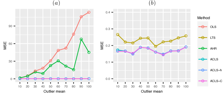
Figure 2: (a) Scenario 2: median of mean square errors vs the outlier mean $a$ for all estimators. (b) Scenario 2: median of mean square errors vs the outlier mean $a$ for LTS, ACLS, ACLS-h and ACLS-C.

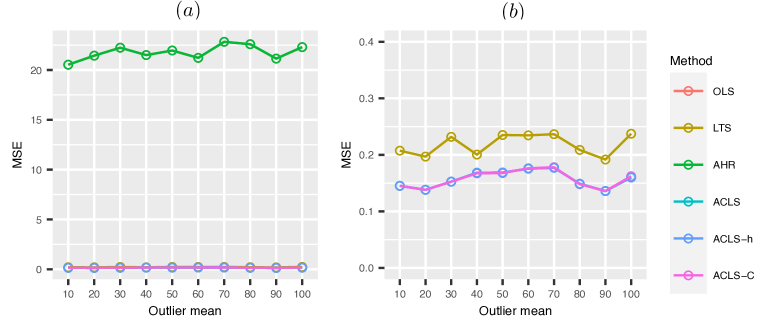
Figure 3: (a) Scenario 3: median of mean square errors vs the outlier mean $a$ for all estimators. (b) Scenario 3: median of mean square errors vs the outlier mean $a$ for LTS, ACLS, ACLS-h and ACLS-C.

Table 1: Simulation results for Scenario 1-3.

		OLS	AHR	LTS	ACLS	ACLS-h	ACLS-C
MMSE	S1	0.1302	0.1302	0.2315	0.1302	0.1303	0.1306
	S2 ($a=50$)	30.6784	22.5611	0.2451	0.1848	0.1849	0.1838
	S3 ($a=100$)	22.2955	22.2955	0.2374	0.1601	0.1600	0.1622
SD	S1	0.8453	0.8453	0.9417	0.8453	0.8453	0.8453

• MMSE, median mean square error; S1, Scenario 1; S2, Scenario 2; S3, Scenario 3.

Table 2: Average CPU time (in seconds) for Scenario 1-3.

	ACLS	ACLS-h	ACLS-C
S1	0.1472	0.1480	2.0134
S2 ($a=50$)	0.4139	0.4322	7.9087
S3 ($a=100$)	0.4811	0.5590	4.7098

• S1, Scenario 1; S2, Scenario 2; S3, Scenario 3.

5.2 The Landscape of Loss Functions

In this section, we visualize the adaptive capped squares loss in the univariate case with one covariate. As expected, the empirical loss is more convex-like as the sample size increases. To be specific, we set the true coefficient $\beta^{*}=5$, and plot the empirical loss $\beta\mapsto\sum_{i=1}^{n}\ell_{\tau}(y_{i}-x_{i}^{\mathrm{\scriptscriptstyle T}}\beta)/n$ with $\tau=\sqrt{n}/\log\log n$ in the following four cases:

1. Case 1: There are no outliers as in Scenario 1;

2. Case 2: There are only $y$-outliers as in Scenario 2 with $a=10$;

3. Case 3: There are both $y$- and $x$-outliers occur as in Scenario 3 with $a=10$, and the contaminated sample size is fixed at $n_{1}=5$;

4. Case 4: There are both $y$- and $x$-outliers occur as in Scenario 3 with $a=10$.

As shown by Figures 4 – 8, the empirical capped squares loss function is locally strongly convex around the global optimum. In Case 1, as $n$ increases the convex region grows and the global optimum is getting closer to $\beta^{*}=5$. Figure 6 shows that although there exists a local minimum when $n$ is small, the loss becomes more convex-like as $n$ increases, and finally this local minimum diminishes. An interesting phenomenon shown in Figure 7 is that this local minimum corresponds to the OLS and the Huber estimator. In other words, both the OLS and the Huber estimators are sensitive to $x$-outliers. In Cases 2 and 4 where the number of outliers also grows, there exists a local minimum around $\beta=1$ when $n$ is small. When $n$ is large, the influence of outliers starts to prevail, and the global optimum is shifted to somewhere around $\beta=1$. In all four cases, the loss function becomes more convex so that any first-order algorithm can identify the global optimum unless initialized very far away, namely, outside the ball $\mathbb{B}_{2}(\tau)$.

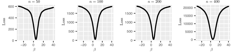
Figure 4: Case 1: Landscape for the adaptive capped least squares loss with (a) $n=50$, (b) $n=100$, (c) $n=200$, (d) $n=400$.

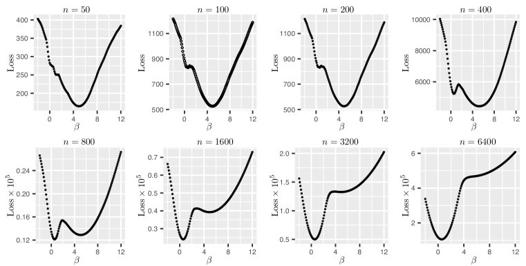
Figure 5: Case 2: Landscape for the adaptive capped least squares loss in Scenario 2.

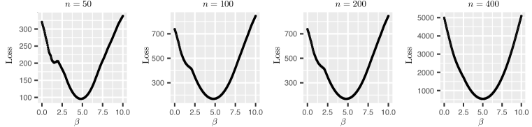
Figure 6: Case 3: Landscape for the adaptive capped least squares loss with (a) $n=50$, (b) $n=100$, (c) $n=200$, (d) $n=400$.

Figure 7: Case 4: OLS and AHR estimators fall in the local local minimum of the adaptive capped least squares loss with $n=300$.

Figure 8: Case 4: Landscape for the adaptive capped least squares loss.

6 Real Data Applications

6.1 NCI-60 Cancer Cell Lines

We apply the proposed method to the NCI-60, a panel of 60 diverse human cancer cell lines. We use two NCI-60 transcript profile datasets, the gene expression dataset and the protein profile dataset. Both datasets can be downloaded from http://discover.nci.nih.gov/cellminer/. The gene expression data were obtained on Affymetrix HG-U133(A-B) chips, and normalized using the guanine cytosine robust multi-array analysis (Wu et al., 2004). The protein profile data based on $162$ antibodies were obtained on reverse-phase protein lysate arrays. One observation had to be removed since all values were missing in the gene expression data, reducing the number of observations to $n=59$. We center all the protein and the gene expression variables to have mean zero.

We pick the KRT19 antibody, which has the largest standard deviation among $162$ antibodies, as the dependent variable. The KRT19 antibody, a type I keratin, also known as Cyfra 21-1, is encoded by the KRT19 gene. Due to its high sensitivity, the KRT19 antibody is the most used biomarker for the tumor cells disseminated in lymph nodes, peripheral blood, and bone marrow of breast cancer patients (Nakata et al., 2004). Sun et al. (2020) has identified seven genes, i.e., MT1E, ARHGAP29, MALL, ANXA3, MAL2, BAMBI and KRT19, that were possibly associated with the KRT19 antibody. We use these seven genes as predictors.

Figure 9: Histograms of the KRT19 antibody expression levels and gene expression levels.

We first plot the histograms of the KRT19 antibody expression levels and seven gene expression levels in Figure 9. The histograms show that the distributions are asymmetric and there are possible outliers in the protein expression data. This could make results based on non-robust methods invalid. Therefore, we apply our methods to examine the predictive performance and statistical significance of the seven genes on predicting the KRT19 antibody. We compare our methods with OLS, AHR and LTS, and report mean absolute prediction errors (MAPEs), the coefficient estimates and the corresponding $p$-values. The MAPE for $\widehat{\beta}$ is defined as ${n}^{-1}\sum_{i=1}^{n}|y_{i}-x_{i}^{\mathrm{\scriptscriptstyle T}}\widehat{\beta}|$. For both our methods and AHR, we set the resistant and robustification parameter as $\tau=\sqrt{59}/\log\log 59$. For ACLS, we run Algorithm 1 100 times and pick the estimator with the smallest adaptive resistant loss. To initialize ACLS-h, we run CPLEX on a subsample of size $\lceil 0.5\times 59\rceil$, followed by gradient descent on the whole data. We then repeat this process $50$ times and pick the estimator with the smallest adaptive resistant loss. We report the average performance of ACLS and ACLS-h from $20$ experiments.

Compared to ACLS-C who achieved loss $5.77$, ACLS and ACLS-h achieved losses of $5.77$ and $5.86$, which are close to the global optimal loss value. This demonstrates the effectiveness of random initialization in ACLS and subsampled initialization in ACLS-h. The MAPEs on the whole dataset are not representative due to the existence of possible outliers. Thus, we calculate MAPEs from a benign subsample of data points, obtained by removing those data with $y$-outliers outside the $25$th and $75$th quantiles. The results are collected in Table 3, and possibly imply that our methods and LTS have favorable predictive performance compared with OLS and AHR.

[flushleft] OLS LTS AHR ACLS ACLS-h ACLS-C MAPE 18.29 8.80 18.09 8.78 8.98 8.78

Table 3: MAPEs of six methods on a subsample of good data points obtained by removing $y$-outliers outside the $25$th and $75$th quantiles.

Table 4 collects the estimates and the corresponding $p$-values. For ACLS and ACLS-h, the median estimates and the corresponding $p$-values, out of $20$ experiments, are reported. The $p$-values are computed using the asymptotic normal distributions, according to Theorem 3.2. To compute the $p$-values, we use the finite sample estimators of $\sigma^{2}$ and $\Sigma_{\tau}$,

$$\widehat{\sigma}^{2}=\frac{1}{n_{e}}\sum_{i}(y_{i}-x_{i}^{\mathrm{\scriptscriptstyle T}}\widehat{\beta}_{\tau})^{2}1(|y_{i}-x_{i}^{\mathrm{\scriptscriptstyle T}}\widehat{\beta}_{\tau}|\leq\tau),~{}\widehat{\Sigma}_{\tau}=\frac{1}{n_{e}}\sum_{i}1(|y_{i}-x_{i}^{\mathrm{\scriptscriptstyle T}}\widehat{\beta}_{\tau}|\leq\tau)x_{i}x_{i}^{\mathrm{\scriptscriptstyle T}},$$

where $n_{e}$ is the number of samples whose absolute residuals are smaller than $\tau$.

The results indicate that MALL, ANXA3, MAL2, BAMBI and KRT19 are statistically significant in predicting the KRT19 antibody expression based on the $p$-values of ACLS, ACLS-h and ACLS-C. ANXA3 is shown to be upregulated in breast cancer tissues and correlated with poor overall survival (Du et al., 2018). It has been reported that MAL2 promotes proliferation, migration, and invasion through regulating epithelial-mesenchymal transition in breast cancer cell lines (Adheesh et al., 2018). Shangguan et al. (2012) has reported that BAMBI transduction disrupted the cytokine network mediating the interaction between mesenchymal stem cells and breast cancer cells. Consequently, BAMBI transduction abolished protumor effects of bone marrow mesenchymal stem cells in vitro and in an orthotopic breast cancer xenograft model, and instead significantly inhibited growth and metastasis of coinoculated cancer. All three implementations of our method have identified MALL as a statistically significant gene in predicting KRT19 antibody expression and thus is possibly associated with breast cancer. This has not been reported by previous studies and is worth further investigation.

[flushleft] Genes MT1E ARHGAP29 MALL ANXA3 MAL2 BAMBI KRT19 $\widehat{\beta}_{\text{OLS}}$ 4.22 -0.32 -0.13 1.48 5.36 -1.88 4.89 $p\text{ value}$ 0.17 0.89 0.96 0.61 0.06 0.42 0.32 $\widehat{\beta}_{\text{AHR}}$ 4.25 -0.42 0.05 1.37 5.19 -1.96 4.96 $p\text{ value}$ $0.00^{*}$ 0.12 0.86 $0.00^{*}$ $0.00^{*}$ $0.00^{*}$ $0.00^{*}$ $\widehat{\beta}_{\text{LTS}}$ -0.12 0.01 -0.01 0.03 -0.14 -0.11 0.03 $p\text{ value}$ 0.12 0.91 0.91 0.59 0.25 $0.03^{*}$ 0.84 $\widehat{\beta}_{\text{ACLS}}$ -0.09 0.05 -0.51 0.21 0.47 -0.16 -0.32 $p$ value 0.32 0.42 $0.00^{*}$ $0.01^{*}$ $0.00^{*}$ $0.02^{*}$ $0.03^{*}$ $\widehat{\beta}_{\text{ACLS-h}}$ -0.09 0.05 -0.51 0.21 0.47 -0.16 -0.32 $p$ value 0.32 0.42 $0.00^{*}$ $0.01^{*}$ $0.00^{*}$ $0.02^{*}$ $0.03^{*}$ $\widehat{\beta}_{\text{ACLS-C}}$ -0.09 0.05 -0.51 0.21 0.47 -0.16 -0.32 $p\text{ value}$ 0.32 0.42 $0.00^{*}$ $0.01^{*}$ $0.00^{*}$ $0.02^{*}$ $0.03^{*}$ Reference $1$ $2$ $3$

Table 4: Estimates and the corresponding $p$-values calculated by six methods, where $p$-values are computed using the asymptotic normal distributions.

• $1$, Du et al. (2018); $2$, Adheesh et al. (2018); $3$, Shangguan et al. (2012).

6.2 Background Recovery in Video Surveillance

We examine the proposed method on the video surveillance dataset from Li et al. (2004). This dataset consists of $n=1546$ frames from a lobby in an office building with illumination changes (switching on/off lights). All frames have resolution $p=128\times 160=20,480$. We first convert all frames to gray scale and then stack each frame as a column of the matrix $(y_{1},\ldots,y_{n})\in\mathbb{R}^{20,480\times 1546}$. The stationary background can often be modeled by a low rank matrix while the moving foreground items are often treated as outliers. We apply our methods to recovery the stationary background.

To utilize the low rank structure of the stationary background, we model each background frame, denoted by $z_{i}$, as

$$z_{i}=m+Us_{i}+\epsilon_{i},~{}1\leq i\leq n,$$

where $m$ is the mean vector, $U\in\mathbb{R}^{p\times q}$ is the orthonormal basis matrix spanning a $q$-dimensional space, $s_{i}$ is the coefficient vector, and $\epsilon_{i}$ is the noise. The observed video frames $y_{i}$ can be seen as contaminated versions of $z_{i}$. To introduce resistance to outliers, we use the adaptive capped least squares regression to estimate the unknowns by solving the following optimization problem

$${\big{\{}\widehat{m},\widehat{U},\{\widehat{s}_{i}\}_{i=1}^{n}\big{\}}=\mathop{\mathrm{argmin}}_{m,U,\{s_{i}\}_{i=1}^{n}}\frac{1}{n}\sum_{i=1}^{n}\ell_{\tau}(\|y_{i}-m-Us_{i}\|_{2}),\quad\textnormal{s.t. }U^{\mathrm{\scriptscriptstyle T}}U=I_{q}},$$ (6.1)

which is then solved by an alternating minimization algorithm. We collect the details of the algorithm in the supplementary material.

In this data example, we choose $q=10$, $\tau=\widehat{\sigma}\cdot\sqrt{n}(\log\log n)^{-1}$ with

$$\widehat{\sigma}=1.4826\times\textnormal{median}\left\{y_{ij}-\textnormal{median}(y_{ij}:1\leq j\leq p):1\leq i\leq n,1\leq j\leq p\right\},$$

where $y_{i}=(y_{i1},\cdots,y_{ip})^{\mathrm{\scriptscriptstyle T}},i=1,\cdots n$. We have $\widehat{\sigma}=0.1512$ and $\tau=2.9811$. The stationary background and moving foreground items of each frame $i$ are then constructed as $\widehat{m}+\widehat{U}\widehat{s}_{i}$ and $(y_{i}-\widehat{m}-\widehat{U}\widehat{s}_{i})\cdot 1(\|y_{i}-\widehat{m}-\widehat{U}\widehat{s}_{i}\|>\tau)$, respectively.

We pick three frames to recover, whose results are collected in Figure 10. The first two rows show the results when the observed frames have a moving person and two standing still people respectively. The third row collects the results for a static scene when some lights are off. For comparison purpose, we also collect the results from ordinary least squares regression, where we replace the capped least squares loss in (6.1) by the quadratic loss. For all cases, our proposed method is able to recover the stationary background without being affected by the moving person, the static people or the illumination change, while the ordinary least squares regression fails in every case.

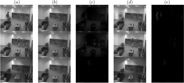
Figure 10: Video surveillance: (a) Original Frames. (b)-(c) Background extraction and outliers from robust regression conducted on adaptive capped least squares regression model. (d)-(e) Background extraction and outliers from the ordinary least squares method.

6.3 Blind Image Inpainting

This section applies the proposed method to blind image inpainting, whose goal is to repair damaged pixels of a given image without knowing the damaged positions as a priori. We first divide the damaged image, possibly after normalization, into $p$ small squared patches, consisting of $\sqrt{n}\times\sqrt{n}$ pixels. We then stack each patch as a column of the signal matrix $Y=(y_{1},\ldots,y_{p})\in\mathbb{R}^{n\times p}$. The damaged pixels of the given image are often treated as outliers in the signal matrix, that is

$$y_{ij}=\begin{cases}u_{ij},&\textnormal{if}\ y_{ij}\text{ is clean};\\ u_{ij}+o_{ij},&\textnormal{if}\ y_{ij}\text{ is a damaged pixel.}\end{cases}$$

where $u_{ij}$ is an undamaged pixel and $o_{ij}$ is an outlier.

Our aim is to apply the proposed method to filtrate corrupted pixels and recover the image using rest undamaged ones. We say an undamaged pixel $u_{i}$ has a sparse representation over a dictionary $D\in\mathbb{R}^{n\times m}$, if we could find a sparse vector $\alpha_{i}\in\mathbb{R}^{m\times 1}$ such than $u_{i}\approx D\alpha_{i}$. The dictionary $D$ is pre-learned from an undamaged picture, and it consists of $m$ basis vectors, referred to as atoms. After learning $D$, we solve $\alpha=(\alpha_{1},\ldots,\alpha_{p})$ by optimize the empirical ACLS loss with Lasso penalties

$$\widehat{\alpha}=\mathop{\mathrm{argmin}}_{\alpha\in\mathbb{R}^{m\times p}}\sum_{i=1}^{p}\ell_{\tau}(y_{i}-D\alpha_{i})+\lambda\sum_{i=1}^{p}\|\alpha_{i}\|_{1},$$ (6.2)

where $\lambda$ is a regularization parameter.

We test the performance of (6.2) on the gray scale Lena image with resolution $d=256\times 256=58,564$. We first normalize all pixel values, 8-bit integers $\in[0,255]$, in the image matrix to real numbers $\in[0,1]$. The columns of the signal matrix is then formed by taking squared patches of size $\sqrt{n}\times\sqrt{n}=15\times 15$ in a sliding manner. We learn the dictionary $D\in\mathbb{R}^{225\times 256}$ from the undamaged image signal matrix as in Mairal et al. (2009). Figure 11 shows the learned dictionary with 256 atoms.

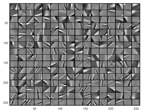
Figure 11: A dictionary with 256 atoms learned on a natural image.

Similar to the video surveillance study, we use alternating minimization algorithm to solve (6.2) with details collected in the supplementary material. The top row of Figure 12 presents two instances for blind image inpainting. In the first instance, we contaminate the original Lena image by changing $300$ pixels value to $0$s where $300$ damaged pixels are uniformly distributed across the image shown in the top-left panel of Figure 12. In the second instance, we contaminate the original image with a manually added curve shown in the top-right panel of Figure 12.

We then apply our method to recover. We use $\tau=c\cdot\widehat{\sigma}\cdot\sqrt{n}(\log\log n)^{-1}$, where $\widehat{\sigma}=1.4826\times\text{median}\{|y_{ij}-\text{median}(y_{i}:1\leq i\leq p)|:1\leq i\leq p,1\leq j\leq n\}$ and $c$ is some constant. In the first instance, $\widehat{\sigma}=0.0349,$ resulting roughly $\tau=0.4$ with $c=0.77$. In the second instance, $\widehat{\sigma}=0.0349,$ resulting $\tau=0.3$ with $c=0.97$. We recover the signal matrix using $Y\odot(1-\widehat{\Delta})+D\widehat{\alpha}\odot\widehat{\Delta}$, where $\odot$ denotes the Hadamard product, $\widehat{\Delta}=[\widehat{\delta}_{ij}]$ and $\widehat{\delta}_{ij}=1(|y_{ij}-[D\widehat{\alpha}_{i}]_{j}|>\tau),i=1,\cdots,p,j=1,\cdots,n$.

The restoration results are presented in the bottom row of Figure 12. For both instances, our proposed method is able to repair the damaged image. We calculate the peak signal to noise ratio (PSNR) of estimates for two cases, which can be used to quantitatively evaluate the quality of the restoration results. The PSNR is defined as,

$$\text{PSNR}(\widehat{x},x)=10\log_{10}\frac{255^{2}}{\frac{1}{d}\sum_{i=1}^{\sqrt{d}}\sum_{j=1}^{\sqrt{d}}(\widehat{x}_{ij}-x_{ij})^{2}},$$

where $x_{ij}$ is the intensity value that from 0 (black) to 255 (white) at $\{i,j\}$ pixel of the damaged image, $\widehat{x}_{ij}$ is the intensity value at $\{i,j\}$ pixel of the recovered image. The PSNR of estimates for two case 1 and case 2 are 47.4590 and 43.7476, respectively.

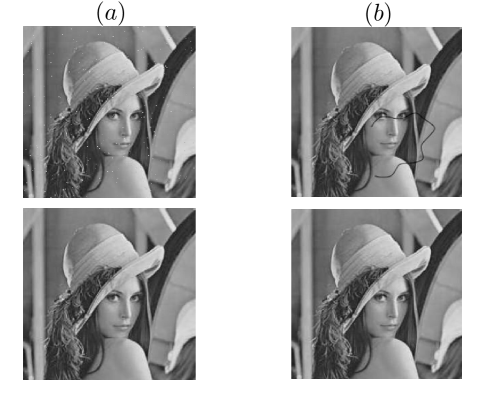
Figure 12: Blind image inpainting: (a) Lena image with random noise and its restoration. (b) Lena image with manually added curve and its restoration.

7 Discussion

This paper proposes the capped least squares regression with an adaptive resistance parameter, hence the name, adaptive capped least squares regression. The key observation is, by taking the resistant parameter to be data-dependent and at a proper order, the proposed estimator automatically achieves high accuracy and high efficiency. Surprisingly, at the same time, it does not lose resistance: the proposed estimator achieves the maximum breakdown point of $1/2$ asymptotically. Computationally, we formulate the problem as a quadratic mixed integer programming problem which can readily solved by CPLEX. To speed up the computation, we propose a randomized gradient descent algorithm. Numerical examples lend strong support to our methodology and theory.

Appendix

Throughout the appendix, we assume all suprema of functions are measurable; otherwise we shall use the essential supremum instead.

Appendix S.1 Proofs for Breakdown Points

This section collects the proofs for Proposition 2.2 and Theorem 2.3.

Proof of Proposition 2.2.

The proof of this proposition is taken from Section 5.13.1 of Maronna et al. (2019). For completeness, we collect it here. Let $g(u)=\mathop{\mathrm{sign}}(x)\left(\tau\wedge|x|\right)$ be the gradient function of the Huber loss function. Then the Huber estimator verifies

$$g(y_{1}-x_{1}^{\mathrm{\scriptscriptstyle T}}\widehat{\beta})x_{1}+\sum_{i=2}^{n}g(y_{i}-x_{i}^{\mathrm{\scriptscriptstyle T}}\widehat{\beta})x_{i}=0.$$ (S.1.1)

Let $y_{1}$ and $x_{1}$ tend to infinity in such a way that $y_{1}/\|x_{1}\|_{2}\rightarrow\infty$. If $\widehat{\beta}$ remained bounded, we would have

$$y_{1}-x_{1}^{\mathrm{\scriptscriptstyle T}}\widehat{\beta}\geq y_{1}-\|x_{1}\|_{2}\|\widehat{\beta}\|_{2}=\|x_{1}\|_{2}\left(\frac{y_{1}}{\|x_{1}\|_{2}}-\|\widehat{\beta}\|_{2}\right)\rightarrow\infty.$$

Since $g$ is nondecreasing, $g(y_{1}-x_{1}^{\mathrm{\scriptscriptstyle T}}\widehat{\beta})$ would tend to $\sup g>0$, and hence the first term in (S.1.1) would tend to infinity, while the sum would remain bounded. This is a contraction. Thus $\widehat{\beta}$ has to be unbounded. This finishes the proof. ∎

The proof of Proposition 2.2 relies on the estimating equations (S.1.1). To prove the breakdown point for ACLS estimator, we take a more general route by directly looking at the losses since the capped least squares loss is not differential.

Proof of Theorem 2.3.

Let $m=n\varepsilon^{*}(\widehat{\beta},\mathcal{Z})$. For every $k\in\mathbb{N}$, there exists a $\mathcal{Z}^{k}\in\mathcal{P}_{m}(\mathcal{Z})$ such that $\|\widehat{\beta}(\mathcal{Z}^{k})\|_{2}>k$. For simplicity, we write $\beta^{k}=\widehat{\beta}(\mathcal{Z}^{k}).$ Without loss of generality, we may assume the first $n-m$ samples in $\mathcal{Z}^{k}$ are uncontaminated. And we have $\|\beta^{k}\|_{2}\rightarrow\infty$. Per the compactness of the unit sphere in $\mathbb{R}^{d}$, we may also suppose that $\theta^{k}=\beta^{k}/\|\beta^{k}\|_{2}$ converges to some point $\theta^{\infty}$, passing to a subsequence otherwise. Then we have

$$\mathcal{L}_{n}\big{(}\beta^{k},\mathcal{Z}^{k}\big{)}\leq\mathcal{L}_{n}\big{(}\beta^{*},\mathcal{Z}^{k}\big{)},$$

or equivalently

$$\sum_{i=1}^{n-m}\ell_{\tau}\big{(}y_{i}-x_{i}^{\mathrm{\scriptscriptstyle T}}\beta^{k}\big{)}+\sum_{i=n-m+1}^{n}\ell_{\tau}\big{(}y_{i}^{k}-(x_{i}^{k})^{\mathrm{\scriptscriptstyle T}}\beta^{k}\big{)}\leq\sum_{i=1}^{n-m}\ell_{\tau}(\epsilon_{i})+\sum_{i=n-m+1}^{n}\ell_{\tau}(\epsilon_{i}^{k}),$$

where $\epsilon_{i}^{k}=y_{i}^{k}-(x_{i}^{k})^{\mathrm{\scriptscriptstyle T}}\beta^{*}.$ Noting that $0\leq\ell_{\tau}(u)\leq\tau^{2}/2$ for all $u$, the above inequality further reduces to

$$\sum_{i=1}^{n-m}\ell_{\tau}\big{(}y_{i}-\|\beta^{k}\|_{2}x_{i}^{\mathrm{\scriptscriptstyle T}}\theta^{k}\big{)}\leq(n-m)\times\frac{1}{n-m}\sum_{i=1}^{n-m}\ell_{\tau}(\epsilon_{i})+m\tau^{2}/2.$$

Under the general position assumption, there are at most $d-1$ samples such that $x_{i}^{\mathrm{\scriptscriptstyle T}}\theta^{\infty}=0$. Denote the collection of such observations by $\mathcal{E}$ with $|\mathcal{E}|\leq d-1$. Hence, by letting $k\rightarrow\infty$, we obtain

$$(n-m-|\mathcal{E}|)\tau^{2}/2+\sum_{i\in\mathcal{E}}\ell_{\tau}(y_{i})\leq(n-m)c_{r}+m\tau^{2}/2,$$

which in turn implies

$$m\geq\frac{n(1-2c_{r}/\tau^{2})-d+1}{2(1-c_{r}/\tau^{2})}.$$

Taking $\tau\rightarrow\infty$ acquires

$$m\geq\left\lceil\frac{n-d+1}{2}\right\rceil=\left\lfloor\frac{n-d+2}{2}\right\rfloor,$$

as desired. ∎

Appendix S.2 Proof of Lemma 3.3

Proof of Lemma 3.3.

Suppose $y=\mu+\epsilon$. Suppose $|\mu-\mu_{\tau}^{*}|\leq\tau/4$, which holds for sufficiency large $\tau$ because $\mu_{\tau}^{*}\rightarrow\mu$. For the loss function $\ell_{\tau}(x)$, we have

$$\ell_{\tau}(x+u)-\ell_{\tau}(x)-\frac{1}{2}u^{2}1(|x|\leq\tau)$$

$$=\frac{1}{2}x^{2}\left(1(|x+u|\leq\tau)-1(|x|\leq\tau)\right)+ux1(|x+u|\leq\tau)$$

$$\qquad+{\frac{1}{2}\tau^{2}\left(1(|x+u|>\tau)-1(|x|>\tau)\right)}+\frac{1}{2}u^{2}\left(1(|x+u|>\tau)-1(|x|>\tau)\right)$$

$$\geq-\frac{1}{2}x^{2}1(\tau-|u|\leq|x|\leq\tau)-\frac{1}{2}\tau^{2}{1(\tau\leq|x|\leq\tau+|u|)}-\frac{1}{2}u^{2}1(\tau-|u|\leq|x|\leq\tau)$$

$$\qquad+ux1(|x+u|\leq\tau),$$

which, by taking $x=y-\mu_{\tau}^{*}$, $u=\Delta$, and $b=\mu-\mu_{\tau}^{*}$, implies

$$\ell_{\tau}(y-\mu_{\tau}^{*}+\Delta)-\ell_{\tau}(y-\mu_{\tau}^{*})-\frac{1}{2}\Delta^{2}1(|y-\mu_{\tau}^{*}|\leq\tau)$$

$$\geq-\frac{1}{2}(y-\mu_{\tau}^{*})^{2}1(\tau-|\Delta|\leq|y-\mu_{\tau}^{*}|\leq\tau)-\frac{1}{2}\tau^{2}1(\tau\leq|y-\mu_{\tau}^{*}|\leq\tau+|\Delta|)$$

$$\qquad-\frac{1}{2}\Delta^{2}1(\tau-|\Delta|\leq|y-\mu_{\tau}^{*}|\leq\tau)+\Delta(y-\mu_{\tau}^{*})1(|y-\mu_{\tau}^{*}+u|\leq\tau)$$

$$=-\frac{1}{2}(y-\mu_{\tau}^{*})^{2}1(\tau-|\Delta|\leq|y-\mu_{\tau}^{*}|\leq\tau)-\frac{1}{2}\tau^{2}1(\tau\leq|y-\mu_{\tau}^{*}|\leq\tau+|\Delta|)$$

$$\qquad-\frac{1}{2}\Delta^{2}1(\tau-|\Delta|\leq|y-\mu_{\tau}^{*}|\leq\tau)+\Delta b(|y-\mu|\leq\tau)$$

$$\qquad+\epsilon\Delta 1(|y-\mu|\leq\tau).$$ (S.2.1)

Suppose $|\Delta|,|b|\leq\tau/4$ such that $|\Delta|+|b|\leq\delta_{0}\leq\tau/2$. Now because $\{\tau-|\Delta|\leq|y-\mu_{\tau}^{*}|\leq\tau\}\subseteq\{\tau-|\Delta|-|b|\leq|\epsilon|\leq\tau+|b|\}$, we have

$$\mathbb{E}(y-\mu_{\tau}^{*})^{2}1(\tau-|\Delta|\leq|y-\mu_{\tau}^{*}|\leq\tau)$$

$$\leq 2\mathbb{E}\left\{(\epsilon^{2}+b^{2})1(\tau-|\Delta|-|b|\leq|\epsilon|\leq\tau+|b|)\right\}$$

$$\leq\frac{2^{3+\eta}L_{0}(|\Delta|+|b|)}{\tau^{3+\eta}}+\frac{2^{5+\eta}L_{0}b^{2}(|\Delta|+|b|)}{\tau^{5+\eta}}.$$

Similarly, we have

$$\mathbb{E}\tau^{2}1(\tau\leq|y-\mu_{\tau}^{*}|\leq\tau+|\Delta|)\leq\frac{L_{0}(|\Delta|+|b|)}{\tau^{3+\eta}},$$

$$\mathbb{E}\Delta^{2}1(\tau-|\Delta|\leq|y-\mu_{\tau}^{*}|\leq\tau)\leq\frac{2^{5+\eta}L_{0}\Delta^{2}(|\Delta|+|b|)}{\tau^{5+\eta}},$$

$$\mathbb{E}\Delta b1(\tau-|\Delta|\leq|y-\mu|\leq\tau)\leq\frac{2^{5+\eta}L_{0}|\Delta b|(|\Delta|+|b|)}{\tau^{5+\eta}}.$$

For the last term in the right hand side of (S.2), we have

$$\mathbb{E}\epsilon\Delta 1(|y-\mu|\leq\tau)=-\mathbb{E}\epsilon\Delta 1(|y-\mu|>\tau)\leq\frac{|\Delta|m_{4+\eta}}{\tau^{3+\eta}}.$$

Let $\mathbb{P}_{n}f=n^{-1}\sum_{i=1}^{n}f_{i}$. Therefore, taking expectation on both sides of the above inequality and summing it over $i$ yield

$$\frac{1}{n}\sum_{i=1}^{n}\left(\mathbb{E}\ell_{\tau}(y_{i}-x_{i}^{\mathrm{\scriptscriptstyle T}}\beta_{\tau}^{*}-x_{i}^{\mathrm{\scriptscriptstyle T}}(\beta-\beta_{\tau}^{*}))-\mathbb{E}\ell_{\tau}(y_{i}-x_{i}^{\mathrm{\scriptscriptstyle T}}\beta_{\tau}^{*})\right)$$

$$\qquad-\frac{1}{2}(\beta-\beta^{*})^{\mathrm{\scriptscriptstyle T}}\frac{1}{n}\sum_{i=1}^{n}x_{i}x_{i}^{\mathrm{\scriptscriptstyle T}}\mathbb{E}1(|y_{i}-x_{i}^{\mathrm{\scriptscriptstyle T}}\beta_{\tau}^{*}|\leq\tau)(\beta-\beta^{*})$$

$$\geq-C\bigg{\{}\frac{\mathbb{P}_{n}\|x\|_{2}(\|\beta-\beta_{\tau}^{*}\|_{2}+\|\beta^{*}-\beta_{\tau}^{*}\|_{2})}{\tau^{3+\eta}}+\frac{\mathbb{P}_{n}\|x\|_{2}\|\beta-\beta_{\tau}^{*}\|_{2}}{\tau^{3+\eta}}$$

$$\qquad\qquad+\frac{\mathbb{P}_{n}\|x\|_{2}^{3}\|\beta^{*}-\beta^{*}_{\tau}\|_{2}^{2}(\|\beta-\beta_{\tau}^{*}\|_{2}+\|\beta^{*}-\beta_{\tau}^{*}\|_{2})}{\tau^{5+\eta}}$$

$$\qquad\qquad+\frac{\mathbb{P}_{n}\|x\|_{2}^{3}\|\beta-\beta_{\tau}^{*}\|_{2}^{2}(\|\beta-\beta_{\tau}^{*}\|_{2}+\|\beta^{*}-\beta_{\tau}^{*}\|_{2})}{\tau^{5+\eta}}$$

$$\qquad\qquad+\frac{\mathbb{P}_{n}\|x\|_{2}^{3}\|\beta-\beta_{\tau}^{*}\|_{2}\|\beta^{*}-\beta_{\tau}^{*}\|_{2}(\|\beta-\beta_{\tau}^{*}\|_{2}+\|\beta^{*}-\beta_{\tau}^{*}\|_{2})}{\tau^{5+\eta}}\bigg{\}},$$

where $C$ only depends on $\eta,\,L_{0}$, and $m_{4+\eta}$. Now since $|x_{i}^{\mathrm{\scriptscriptstyle T}}(\beta-\beta_{\tau}^{*})|\leq\tau/4$, we have

$$\mathbb{E}1(|y_{i}-x_{i}^{\mathrm{\scriptscriptstyle T}}\beta_{\tau}^{*}|\leq\tau)\geq\mathbb{E}1(|\epsilon_{i}|\leq 3\tau/4),$$

and thus $\rho_{\tau}=\lambda_{\min}\left(n^{-1}\sum_{i=1}^{n}x_{i}x_{i}^{\mathrm{\scriptscriptstyle T}}1(|\epsilon_{i}|\leq 3\tau/4)\right)>0.$ Now if $\sqrt{d}/\tau^{3+\eta}\leq c\|\beta-\beta_{\tau}^{*}\|_{2}$ and $\sqrt{d^{3}}/\tau^{5+\eta}\leq c\|\beta-\beta_{\tau}^{*}\|_{2}^{-1}$ for $c$, depending only on $C$ and $\rho_{\tau}$, sufficiently small, we have

$$\frac{1}{n}\sum_{i=1}^{n}\left(\mathbb{E}\ell_{\tau}(y_{i}-x_{i}^{\mathrm{\scriptscriptstyle T}}\beta_{\tau}^{*}-x_{i}^{\mathrm{\scriptscriptstyle T}}(\beta-\beta_{\tau}^{*}))-\mathbb{E}\ell_{\tau}(y_{i}-x_{i}^{\mathrm{\scriptscriptstyle T}}\beta_{\tau}^{*})\right)\geq\frac{1}{4}\rho_{\tau}\|\beta-\beta^{*}\|_{2},$$

as desired.

∎

Appendix S.3 Proof for Consistency

To prove consistency, we first establish the uniform law of large numbers for the empirical loss, namely, $\sup_{\beta\in\mathbb{R}^{d}}\big{|}(1/n)\sum_{i=1}^{n}\ell_{\tau}(y_{i}-x_{i}^{\mathrm{\scriptscriptstyle T}}\beta)-(1/n)\sum_{i=1}^{n}\mathbb{E}\ell_{\tau}(y_{i}-x_{i}^{\mathrm{\scriptscriptstyle T}}\beta)\big{|}$.

Theorem S.3.1.

With probability at least $1-\delta$, we have

$$\sup_{\beta\in\mathbb{R}^{d}}\left|\frac{1}{n}\sum_{i=1}^{n}\ell_{\tau}(y_{i}-x_{i}^{\mathrm{\scriptscriptstyle T}}\beta)-\frac{1}{n}\sum_{i=1}^{n}\mathbb{E}\ell_{\tau}(y_{i}-x_{i}^{\mathrm{\scriptscriptstyle T}}\beta)\right|\leq C\tau^{2}\left(\sqrt{\frac{d}{n}}+\ \sqrt{\frac{\log{1}/{\delta}}{n}}\right),$$

where $C>0$ is a universal constant.

Proof of Theorem S.3.1.

We first fix $\tau$ and thus the loss function $\ell_{\tau}(\cdot)$. Let

$$\mathcal{V}=\left\{f_{\beta}(x,\epsilon)=\epsilon-x^{\mathrm{\scriptscriptstyle T}}(\beta-\beta^{*}):\beta\in\mathbb{R}^{d}\right\}$$

be a class of functions $\mathbb{R}^{d}\times\mathbb{R}\to\mathbb{R}$. Given a function $f\in\mathcal{V}$, we write $\mathbb{P}_{n}f=n^{-1}\sum_{i=1}^{n}f(z_{i})$ and $\mathbb{P}f={n}^{-1}\sum_{i=1}^{n}\mathbb{E}f(z_{i})$, where $z_{i}=(x_{i},\epsilon_{i})$. Moreover, write $\left\|\mathbb{P}_{n}-\mathbb{P}\right\|_{\mathcal{F}}=\sup_{f\in\mathcal{F}}|\mathbb{P}_{n}f-\mathbb{P}f|.$ Under this notation, we have

$$\sup_{\beta\in\mathbb{R}^{d}}\left|\frac{1}{n}\sum_{i=1}^{n}\ell_{\tau}(y_{i}-x_{i}^{\mathrm{\scriptscriptstyle T}}\beta)-\frac{1}{n}\sum_{i=1}^{n}\mathbb{E}\ell_{\tau}(y_{i}-x_{i}^{\mathrm{\scriptscriptstyle T}}\beta)\right|=\sup_{g\in\ell_{\tau}\circ\mathcal{V}}\left|\mathbb{P}_{n}g-\mathbb{P}g\right|.$$

Applying Lemma S.5.1 to the function class $\ell_{\tau}\circ\mathcal{V}$, which is $\ell_{\tau}\circ\mathcal{V}$ is $\tau^{2}/2$-bounded, yields that

$$\left\|\mathbb{P}_{n}-\mathbb{P}\right\|_{\mathcal{F}}\leq\mathbb{E}\|\mathbb{P}_{n}-\mathbb{P}\|_{\mathcal{F}}+\frac{\tau^{2}}{2}\sqrt{\frac{2\log(1/\delta)}{n}},$$ (S.3.1)

with probability at least $1-\delta$. We then upper bound the mean $\mathbb{E}\|\mathbb{P}_{n}-\mathbb{P}\|_{\mathcal{F}}$ using Dudley’s entropy integral bound as summarized in Lemma S.5.2.

To proceed, we need to control the metric entropy of $\ell_{\tau}\circ\mathcal{V}$. Note first that the functional class $\mathcal{V}$ is a $d$-dimensional vector space. By Lemma 2.6.15 of van der Vaart and Wellner (1986), $\mathcal{V}$ has a VC-subgraph dimension at most $\nu=\textnormal{vc}(\mathcal{V})\leq d+2.$ Here the notion of VC-subgraph dimension is defined in van der Vaart and Wellner (1986). We rewrite the loss function $\ell_{\tau}(u)$ as

$$\ell_{\tau}(u)=\ell_{\tau}^{+}(u)+\ell_{\tau}^{-}(u),~{}\text{where}~{}\ell_{\tau}^{+}(u)=\ell_{\tau}(u)1(u\geq 0)\text{ and }\ell_{\tau}^{-}(u)=\ell_{\tau}(u)1(u<0).$$

Then, $\ell_{\tau}(y-x^{\mathrm{\scriptscriptstyle T}}\beta)$ can be written as the sum of two composite loss functions

$$\ell_{\tau}(y-x^{\mathrm{\scriptscriptstyle T}}\beta)=\ell_{\tau}^{+}\circ f+\ell_{\tau}^{-}\circ f,~{}\text{where}~{}f=f_{\beta}\in\mathcal{V}.$$

Since $\ell_{\tau}^{+}$ is an increasing function, by Lemma 2.6.15 of van der Vaart and Wellner (1986), $\ell_{\tau}^{+}\circ\mathcal{V}$ has VC-subgraph dimension of at most $d+2$. Similarly, $\ell_{\tau}^{-}\circ\mathcal{V}$ has VC-subgraph dimension of most $d+2$. Applying Lemma 2.6.7 in van der Vaart and Wellner (1986) yields that, for any probability measure $Q$ and $0<s<1$,

$$N(s\tau^{2}/2,\ell_{\tau}^{+}\circ\mathcal{V},L_{2}(Q)) \leq K(d+2)(16e)^{d+2}\left(\frac{1}{s}\right)^{2(d+1)},$$

$$N(s\tau^{2}/2,\ell_{\tau}^{-}\circ\mathcal{V},L_{2}(Q)) \leq K(d+2)(16e)^{d+2}\left(\frac{1}{s}\right)^{2(d+1)},$$

where $K>0$ is a universal constant. By elementary calculations,

$$N(s\tau^{2},\ell_{\tau}^{+}\circ\mathcal{V}+\ell_{\tau}^{-}\circ\mathcal{V},L_{2}(Q)) \leq N(s\tau^{2}/2,\ell_{\tau}^{+}\circ\mathcal{V},L_{2}(Q))\times N(s\tau^{2}/2,\ell_{\tau}^{+}\circ\mathcal{V},L_{2}(Q))$$

$$\leq\left\{K(d+2)(16e)^{d+2}\left(\frac{1}{s}\right)^{2(d+1)}\right\}^{2}=:M(d,s).$$

Since $\ell_{\tau}\circ\mathcal{V}$ is a subclass of $\ell_{\tau}^{+}\circ\mathcal{V}+\ell_{\tau}^{-}\circ\mathcal{V}$, the covering number of $\ell_{\tau}\circ\mathcal{V}$ is smaller than that of $\ell_{\tau}^{+}\circ\mathcal{V}+\ell_{\tau}^{-}\circ\mathcal{V}$. If $d\geq 1$, there exists some universal constant $C_{1}$ such that $1+\log M(d,s)\leq C_{1}d\log(e/s)$, for any $0<s<1$. Applying Lemma S.5.2 with $F=\tau^{2}/2$ acquires

$$\mathbb{E}\bigl{\{}\sqrt{n}\|\mathbb{P}_{n}-\mathbb{P}\|_{\mathcal{F}}\bigr{\}} \leq C\tau^{2}\int_{0}^{1}\sqrt{1+\log N(s\tau^{2},\ell_{\tau}\circ\mathcal{V},L_{2}(\mathbb{P}_{n}))}\textnormal{d}s$$

$$\leq C\tau^{2}\sqrt{C_{1}d}\int_{0}^{1}\sqrt{\log(e/s)}\,\textnormal{d}s\leq C_{2}\tau^{2}\sqrt{d},$$

where $C_{2}$ is a universal constant. Together with (S.3.1), we obtain that, for any $n\geq 1$ and $0\leq\delta\leq 1$,

$$\left\|\mathbb{P}_{n}-\mathbb{P}\right\|_{\mathcal{F}}\leq 2C_{2}\tau^{2}\sqrt{\frac{d}{n}}+\frac{\tau^{2}}{2}\sqrt{\frac{2\log(1/\delta)}{n}},$$

with probability at least $1-\delta$. This completes the proof. ∎

Now we are ready to prove Theorem 3.1.

Proof of Theorem 3.1.

To begin with, we have the following basic inequality

$$0\leq\mathcal{L}(\widehat{\beta}_{\tau})-\mathcal{L}(\beta^{*}_{\tau}) =\mathcal{L}(\widehat{\beta}_{\tau})-\mathcal{L}_{n}(\widehat{\beta}_{\tau})+\mathcal{L}_{n}(\widehat{\beta}_{\tau})-\mathcal{L}_{n}(\beta^{*}_{\tau})+\mathcal{L}_{n}(\beta^{*}_{\tau})-\mathcal{L}(\beta^{*}_{\tau})$$

$$\leq\mathcal{L}(\widehat{\beta}_{\tau})-\mathcal{L}_{n}(\widehat{\beta}_{\tau})+\mathcal{L}_{n}(\beta^{*}_{\tau})-\mathcal{L}(\beta^{*}_{\tau}),$$

where the last inequality is due to the fact that $\mathcal{L}_{n}(\widehat{\beta}_{\tau})\leq\mathcal{L}_{n}(\beta^{*}_{\tau}).$ Rearranging the terms gives

$$0 \leq-\mathbb{P}\bigl{\{}\ell_{\tau}(y-x^{\mathrm{\scriptscriptstyle T}}\beta^{*}_{\tau})-\ell_{\tau}(y-x^{\mathrm{\scriptscriptstyle T}}\widehat{\beta}_{\tau})\bigr{\}}$$

$$\leq-(\mathbb{P}_{n}-\mathbb{P})\bigl{\{}\ell_{\tau}(y-x^{\mathrm{\scriptscriptstyle T}}\widehat{\beta}_{\tau})-\ell_{\tau}(y-x^{\mathrm{\scriptscriptstyle T}}\beta^{*}_{\tau})\bigr{\}}$$

$$\leq 2\sup_{\beta\in\mathbb{R}^{d}}(\mathbb{P}_{n}-\mathbb{P})\ell_{\tau}(y-x^{\mathrm{\scriptscriptstyle T}}\beta)$$

$$\lesssim\tau^{2}\sqrt{\frac{d+\log(1/\delta)}{n}}~{}\text{with probability}\geq 1-\delta$$

$$\to 0~{}\mbox{ as }~{}n\to\infty,$$

provided that $\tau^{4}d\rightarrow o(n)$, or equivalently $\tau=\text{o}((n/d)^{1/4})$. By Assumption 2, for any fixed $\varepsilon>0$, there exists some $\eta>0$ such that

$$\inf_{\beta:\|\beta-\beta_{\tau}^{*}\|_{2}\geq\varepsilon}\mathcal{L}(\beta)>\mathcal{L}(\beta_{\tau}^{*})-\eta,$$

which further implies

$$\mathbb{P}\bigl{(}\big{\|}\widehat{\beta}_{\tau}-\beta^{*}_{\tau}\big{\|}_{2}\geq\varepsilon\bigr{)}\leq\mathbb{P}\bigl{\{}\mathcal{L}(\widehat{\beta}_{\tau})>\mathcal{L}(\beta^{*}_{\tau})-\eta\bigr{\}}\rightarrow 0.$$

This proves $\big{\|}\widehat{\beta}_{\tau}-\beta^{*}_{\tau}\big{\|}_{2}\overset{\mathbb{P}}{\to}0$. Taking into account the fact that $\beta_{\tau}^{*}\rightarrow\beta^{*}$ as $\tau\rightarrow\infty$, we obtain $\widehat{\beta}_{\tau}\overset{\mathbb{P}}{\to}\beta^{*}$, as claimed. ∎

Appendix S.4 Proof for Asymptotic Normality

This section presents the proof of Theorem 3.2. We first need two results on the bias and convergence rate of the ACLS estimator.

Lemma S.4.1 (Bias).

Suppose that Assumptions 3 – 5 hold and $m_{4+\eta}<\infty$. Then

$$\big{\|}\beta^{*}_{\tau}-\beta^{*}\big{\|}_{2}\lesssim\kappa_{\ell}^{-1}d^{1/2}\tau^{-(3+\eta)}.$$

Provided that $\tau\gtrsim n^{1/(6+2\eta)}$, we have $\|\beta^{*}_{\tau}-\beta^{*}\|_{2}\lesssim\kappa_{\ell}^{-1}\sqrt{{d}/{n}}.$

Theorem S.4.2 (Convergence Rate).

Suppose that Assumptions 3 – 5 hold with $m_{4+\eta}$ exists. Moreover, assume that $n\gtrsim d^{3}$ and $\tau\geq n^{\frac{1}{2(1+\eta)}}$. If $\widehat{\beta}_{\tau}\overset{\mathbb{P}}{\to}\beta_{\tau}^{*}$, then

$$\|\widehat{\beta}_{\tau}-\beta^{*}_{\tau}\|_{2}=\text{O}_{\mathbb{P}}\bigl{(}\kappa_{\ell}^{-1}\sqrt{d/n}\bigr{)}.$$

Consequently, $\|\widehat{\beta}_{\tau}-\beta^{*}\|_{2}=\text{O}_{\mathbb{P}}(\kappa_{\ell}^{-1}\sqrt{d/n})$.

Proof of Theorem 3.2.

By Theorem S.4.2, we have $\|\widehat{\beta}_{\tau}-\beta^{*}\|_{2}=\text{O}_{\mathbb{P}}((d/n)^{1/2})$. For every $\beta\in\mathbb{R}^{d}$, write $t=\beta-\beta^{*}$, and define

$$\Sigma_{\tau}(t)=\frac{1}{n}\sum_{i=1}^{n}\mathbb{E}\{x_{i}x_{i}^{\mathrm{\scriptscriptstyle T}}1(|\epsilon_{i}-x_{i}^{\mathrm{\scriptscriptstyle T}}t|\leq\tau)\},$$

$$D_{n}(t)=\frac{1}{n}\sum_{i=1}^{n}\{\ell_{\tau}(\epsilon_{i}-x_{i}^{\mathrm{\scriptscriptstyle T}}t)-\ell_{\tau}(\epsilon_{i})\}.$$

Similarly to the bias analysis, we can show that, for any $t$ that satisfies $\|t\|_{2}\leq r\lesssim(d/n)^{1/2}$, a neighborhood of $0$,

$$\mathbb{E}D_{n}(t)=\frac{1}{2}t^{\mathrm{\scriptscriptstyle T}}\Sigma_{\tau}(t)t+\text{O}\biggl{(}\frac{\|t\|_{2}\mathbb{P}_{n}\|x\|_{2}}{\tau^{3+\eta}}\biggr{)}=\frac{1}{2}t^{\mathrm{\scriptscriptstyle T}}\Sigma_{\tau}(t)t+\text{o}\bigl{(}\|t\|_{2}^{2}\bigr{)}$$

as long as $\tau^{-3-\eta}\mathbb{P}_{n}\|x\|_{2}=\text{o}(\|t\|_{2})$, which holds if $n=\text{o}(\tau^{6+2\eta})$ and is implied by $\tau\propto n^{1/(2+\eta)}$. For $t$ in a shrinking neighborhood of $0$, let $\tau>0$ satisfy $\max_{1\leq i\leq n}|x_{i}^{\mathrm{\scriptscriptstyle T}}t|\leq\tau/2$. Then, we have

$$\|\Sigma_{\tau}(t)-\Sigma_{\tau}\|_{2}$$

$$=\Biggl{\|}{\frac{1}{n}\sum_{i=1}^{n}\mathbb{E}\bigl{\{}x_{i}x_{i}^{\mathrm{\scriptscriptstyle T}}1(|\epsilon_{i}-x_{i}^{\mathrm{\scriptscriptstyle T}}t|\leq\tau)\bigr{\}}-\frac{1}{n}\sum_{i=1}^{n}\mathbb{E}\bigl{\{}x_{i}x_{i}^{\mathrm{\scriptscriptstyle T}}1(|\epsilon_{i}|\leq\tau)\bigr{\}}}\Biggr{\|}_{2}$$

$${\leq}\Biggl{\|}\frac{1}{n}\sum_{i=1}^{n}x_{i}x_{i}^{\mathrm{\scriptscriptstyle T}}\,\mathbb{E}\bigl{\{}{1(\tau-|x_{i}^{\mathrm{\scriptscriptstyle T}}t|\leq|\epsilon_{i}|\leq\tau+|x_{i}^{\mathrm{\scriptscriptstyle T}}t|)}\bigr{\}}\Biggr{\|}_{2}$$

$$\leq\left\|\frac{1}{n}\sum_{i=1}^{n}x_{i}x_{i}^{\mathrm{\scriptscriptstyle T}}\,\mathbb{P}(\tau/2\leq|\epsilon_{i}|\leq 3\tau/2)\right\|_{2}\leq\frac{2m_{1}}{\tau}\|\Sigma\|_{2}\rightarrow 0,$$

provided that $\tau\rightarrow\infty$. It follows that

$$\mathbb{E}D_{n}(t)=\frac{1}{2}t^{\mathrm{\scriptscriptstyle T}}\Sigma_{\tau}t+\text{o}\bigl{(}\|t\|_{2}^{2}\bigr{)}.$$

Next, following a similar proof of Theorem S.4.2, we obtain the following maximal inequality

$$\mathbb{E}\sup_{\|t\|_{2}\leq r}|D_{n}(t)-\mathbb{E}D_{n}(t)|\lesssim r\sqrt{\frac{d}{n}},$$

which further implies

$$|D_{n}(t)-\mathbb{E}D_{n}(t)|=\text{O}_{\mathbb{P}}\bigl{(}r(d/n)^{1/2}\bigr{)}$$

uniformly over $t$ satisfying $\|t\|_{2}\leq r$. Direct calculation yields

$$\mathbb{E}\{\ell_{\tau}(\epsilon_{i}-x_{i}^{\mathrm{\scriptscriptstyle T}}t)-\ell_{\tau}(\epsilon_{i})\}$$

$$=\mathbb{E}\left\{\frac{1}{2}\epsilon_{i}^{2}1(|\epsilon_{i}-x_{i}^{\mathrm{\scriptscriptstyle T}}t|\leq\tau)-\frac{1}{2}\epsilon_{i}^{2}1(|\epsilon_{i}|\leq\tau)\right\}-\mathbb{E}\bigg{\{}\epsilon_{i}x_{i}^{\mathrm{\scriptscriptstyle T}}t{1(|\epsilon_{i}-x_{i}^{\mathrm{\scriptscriptstyle T}}t|\leq\tau)}\bigg{\}}$$

$$\quad+\mathbb{E}\bigg{\{}(x_{i}^{\mathrm{\scriptscriptstyle T}}t)^{2}1(|\epsilon_{i}-x_{i}^{\mathrm{\scriptscriptstyle T}}t|\leq\tau)\bigg{\}}+\mathbb{E}\left\{\frac{1}{2}\tau^{2}1(|\epsilon_{i}-x_{i}^{\mathrm{\scriptscriptstyle T}}t|>\tau)-\frac{1}{2}\tau^{2}1(|\epsilon_{i}|>\tau)\right\}.$$

Define the remainder

$$R_{i}(t)=\ell_{\tau}(\epsilon_{i}-x_{i}^{\mathrm{\scriptscriptstyle T}}t)-\ell_{\tau}(\epsilon_{i})+{\psi_{\tau}(\epsilon_{i})}x_{i}^{\mathrm{\scriptscriptstyle T}}t.$$

By the definition of $\ell_{\tau}$, we have

$$R_{i}(t) =\frac{1}{2}\epsilon_{i}^{2}\left\{1(|\epsilon_{i}-x_{i}^{\mathrm{\scriptscriptstyle T}}t|\leq\tau)-1(|\epsilon_{i}|\leq\tau)\right\}+\epsilon_{i}x_{i}^{\mathrm{\scriptscriptstyle T}}t\left({1(|\epsilon_{i}|\leq\tau)-1(|\epsilon_{i}-x_{i}^{\mathrm{\scriptscriptstyle T}}t|\leq\tau)}\right)$$

$$\quad+(x_{i}^{\mathrm{\scriptscriptstyle T}}t)^{2}1(|\epsilon_{i}-x_{i}^{\mathrm{\scriptscriptstyle T}}t|\leq\tau)+\frac{1}{2}\tau^{2}\left\{1(|\epsilon_{i}-x_{i}^{\mathrm{\scriptscriptstyle T}}t|>\tau)-1(|\epsilon_{i}|>\tau)\right\},$$

which has an envelope $F:\mathbb{R}^{d+1}\to\mathbb{R}$ given by

$$F(z_{i}) =\frac{1}{2}\epsilon_{i}^{2}1(\tau-|x_{i}^{\mathrm{\scriptscriptstyle T}}t|\leq|\epsilon_{i}|\leq\tau+|x_{i}^{\mathrm{\scriptscriptstyle T}}t|)+{|\epsilon_{i}x_{i}^{\mathrm{\scriptscriptstyle T}}t|1(\tau-|x_{i}^{\mathrm{\scriptscriptstyle T}}t|\leq\epsilon_{i}\leq\tau+|x_{i}^{\mathrm{\scriptscriptstyle T}}t|)}$$

$$\quad+(x_{i}^{\mathrm{\scriptscriptstyle T}}t)^{2}1(|\epsilon_{i}-x_{i}^{\mathrm{\scriptscriptstyle T}}t|\leq\tau)+\frac{1}{2}\tau^{2}1(\tau-|x_{i}^{\mathrm{\scriptscriptstyle T}}t|\leq|\epsilon_{i}|\leq\tau+|x_{i}^{\mathrm{\scriptscriptstyle T}}t|)$$

for $z_{i}=(x_{i},\epsilon_{i})$. For $\|t\|_{2}\leq r\leq\tau/(2\|x_{i}\|_{2})\wedge 1$ and $\tau\geq 1$,

$$\mathbb{E}F^{2} \lesssim\mathbb{E}\left\{\epsilon_{i}^{4}1(\tau-|x_{i}^{\mathrm{\scriptscriptstyle T}}t|\leq|\epsilon_{i}|\leq\tau+|x_{i}^{\mathrm{\scriptscriptstyle T}}t|)+\epsilon_{i}^{2}(x_{i}^{\mathrm{\scriptscriptstyle T}}t)^{2}1(\tau-|x_{i}^{\mathrm{\scriptscriptstyle T}}t|\leq\epsilon_{i}\leq\tau+|x_{i}^{\mathrm{\scriptscriptstyle T}}t|)\right\}$$

$$\quad+\mathbb{E}\left\{(x_{i}^{\mathrm{\scriptscriptstyle T}}t)^{4}1(|\epsilon_{i}-x_{i}^{\mathrm{\scriptscriptstyle T}}t|\leq\tau)+\tau^{4}1(\tau-|x_{i}^{\mathrm{\scriptscriptstyle T}}t|\leq|\epsilon_{i}|\leq\tau+|x_{i}^{\mathrm{\scriptscriptstyle T}}t|)\right\}$$

$$\lesssim\frac{L_{0}|x_{i}^{\mathrm{\scriptscriptstyle T}}t|}{\tau^{1+\eta}}+\frac{L_{0}|x_{i}^{\mathrm{\scriptscriptstyle T}}t|^{2}}{\tau^{3+\eta}}+(x_{i}^{\mathrm{\scriptscriptstyle T}}t)^{4}\lesssim\|t\|_{2}^{2},$$

provided that $\tau^{1+\eta}\gtrsim\|x_{i}\|_{2}/\|t\|_{2}$, $\tau^{2+\eta}\gtrsim\|x_{i}\|_{2}^{2}$ and $\|x_{i}\|_{2}^{4}\|t\|_{2}^{2}\lesssim 1$, all of which hold if $n\gtrsim d^{3}$ and $\tau\gtrsim n^{1/(2+2\eta)}$.

Now we consider to bound the local fluctuation uniformly

$$\sup_{t:\|t\|_{2}\leq r}\Biggl{|}\frac{1}{\sqrt{n}}\sum_{i=1}^{n}\left\{R_{i}(t)-\mathbb{E}R_{i}(t)\right\}\Biggr{|}.$$

Similar to the proof of Theorem S.3.1, we write

$$R_{i}(t)=\ell_{\tau}^{+}(\epsilon_{i}-x_{i}^{\mathrm{\scriptscriptstyle T}}t)+\ell_{\tau}^{-}(\epsilon_{i}-x_{i}^{\mathrm{\scriptscriptstyle T}}t)+\psi_{\tau}(\epsilon_{i})x_{i}^{\mathrm{\scriptscriptstyle T}}t-\ell_{\tau}(\epsilon_{i}).$$

This implies that the covering number for the class of functions $R_{i}(t)$, denoted by $\mathcal{G}_{r}$, is upper bounded by

$$N(s\|F\|_{Q,2},\mathcal{G}_{r},\|\cdot\|_{Q,2}) \leq\left\{K(d+2)(16e)^{d+2}\left(\frac{1}{s}\right)^{2(d+1)}\right\}^{3}.$$

Recall that $\mathbb{P}f=\mathbb{E}\mathbb{P}_{n}f$. Applying the maximum inequality in Lemma S.5.4 with $\psi(x)=x^{1+\eta/4}$ and $\lambda=1$ acquires

$$B:=\sqrt{\mathbb{E}\max_{1\leq i\leq n}F^{2}(z_{i})}\lesssim(\mathbb{P}F^{2+\eta/2})^{\frac{1}{2+\eta/2}}=:n^{\frac{1}{2+\eta/2}}\|F\|_{\mathbb{P},2+\eta/2}.$$

Applying Lemma S.5.3 with $\delta=\sqrt{\mathbb{P}F^{2}}\lesssim\|t\|_{2}$ yields

$$\mathbb{E}\sup_{\|t\|_{2}\leq r}\sqrt{n}|\mathbb{P}_{n}R(t)-\mathbb{P}R(t)|$$

$$\lesssim J(\delta,F,\mathcal{F})\|F\|_{\mathbb{P},2}+\frac{BJ^{2}(\delta,F,\mathcal{F})}{\delta^{2}\sqrt{n}}$$

$$\lesssim\|F\|_{\mathbb{P},2}\left\{J(\delta,F,\mathcal{F})+\frac{BJ^{2}(\delta,F,\mathcal{F})}{\delta^{2}\sqrt{n}}\right\}$$

$$\lesssim\|F\|_{\mathbb{P},2}\left\{J(\delta,F,\mathcal{F})+n^{-\frac{\eta}{8+2\eta}}\frac{\|F\|_{\mathbb{P},2+\eta/2}J^{2}(\delta,F,\mathcal{F})}{\|F\|_{\mathbb{P},2}\delta^{2}}\right\}$$

$$\lesssim\|F\|_{\mathbb{P},2}J(\delta,F,\mathcal{F}).$$

Similar to the proof of Theorem S.3.1, we shall have $J(\delta,F,\mathcal{F})\lesssim\|F\|_{\mathbb{P},2}\sqrt{d}$. This implies that uniformly in a shrinking neighborhood of $0$,

$$\sqrt{n}|\mathbb{P}_{n}R(t)-\mathbb{P}R(t)|=\text{O}_{\mathbb{P}}\bigl{(}\|t\|_{2}^{2}\sqrt{d}\bigr{)}=\text{o}_{\mathbb{P}}\bigl{(}\|t\|_{2}\bigr{)},$$

if $n\gg d^{2}$ which is implied by $n\gtrsim d^{3}$. Hence

$$D_{n}(t)=\mathbb{E}D_{n}(t)+t^{\mathrm{\scriptscriptstyle T}}\mathbb{P}_{n}\psi_{\tau}(\epsilon)x+\text{o}_{\mathbb{P}}\bigl{(}\|t\|_{2}/\sqrt{n}\bigr{)}.$$

Let $t_{n}=\widehat{\beta}_{\tau}-\beta^{*}$. Thus

$$D_{n}(t_{n}) =\mathbb{E}D_{n}(t_{n})+t_{n}^{\mathrm{\scriptscriptstyle T}}\mathbb{P}_{n}\psi_{\tau}(\epsilon)x+\text{o}_{\mathbb{P}}\bigl{(}\|t_{n}\|_{2}/\sqrt{n}\bigr{)}$$

$$=\frac{1+\text{o}_{\mathbb{P}}(1)}{2}\left\|\Sigma_{\tau}^{1/2}t_{n}-{\Sigma_{\tau}^{-1/2}\mathbb{P}_{n}\psi(\epsilon)x}\right\|_{2}^{2}-\frac{\|\Sigma_{\tau}^{-1/2}\mathbb{P}_{n}\psi(\epsilon)x\|_{2}^{2}}{2}+\text{o}_{\mathbb{P}}(n^{-1}).$$

By the optimality of $\widehat{\beta}_{\tau}$, $D_{n}(t_{n})\leq D_{n}(\Sigma_{\tau}^{-1/2}\mathbb{P}_{n}\psi_{\tau}(\epsilon)x)$. Putting together the pieces, we conclude that

$$\frac{1+\text{o}_{\mathbb{P}}(1)}{2}\left\|\Sigma_{\tau}^{1/2}t_{n}-{\Sigma_{\tau}^{-1/2}\mathbb{P}_{n}\psi(\epsilon)x}\right\|_{2}^{2}-\frac{\|\Sigma_{\tau}^{-1/2}\mathbb{P}_{n}\psi(\epsilon)x\|_{2}^{2}}{2}+\text{o}_{\mathbb{P}}(n^{-1})$$

$$\leq-\frac{\|\Sigma_{\tau}^{-1/2}\mathbb{P}_{n}\psi_{\tau}(\epsilon)x\|_{2}^{2}}{2}+\text{o}_{\mathbb{P}}(n^{-1}),$$

or equivalently

$$\sqrt{n}(\widehat{\beta}_{\tau}-\beta^{*})=\frac{1}{\sqrt{n}}\sum_{i=1}^{n}\Sigma_{\tau}^{-1}\psi_{\tau}(\epsilon_{i})x_{i}+\Delta_{n},$$

where $\|\Delta_{n}\|_{2}=\text{o}_{\mathbb{P}}(1).$

∎

S.4.1 Proof of Technical Results

This section collects the proofs for Lemma S.4.1 and Theorem S.4.2.

Proof of Lemma S.4.1.

Because $\beta^{*}_{\tau}\rightarrow\beta^{*}$ as $\tau\rightarrow\infty$, for any $r>0$, we have $\|\beta^{*}-\beta^{*}_{\tau}\|_{2}\leq r$ for sufficiently large $\tau$. For simplicity, for a fixed predictor $x$ with $\|x\|_{2}\leq C_{x}d^{1/2}$, write $\mu=x^{\mathrm{\scriptscriptstyle T}}\beta$, $\mu^{*}=x^{\mathrm{\scriptscriptstyle T}}\beta^{*}$ and $\mu^{*}_{\tau}=x^{\mathrm{\scriptscriptstyle T}}\beta^{*}_{\tau}$. Recall that $\epsilon$ denotes the model error satisfying $\mathbb{E}\epsilon=0$. By direction calculations, we have

$$\mathbb{E}\ell_{\tau}\left(\epsilon\right)-\mathbb{E}\ell_{\tau}\left(\epsilon+\mu^{*}-\mu^{*}_{\tau}\right)$$

$$=\mathbb{E}\left\{\frac{1}{2}\epsilon^{2}1(|\epsilon|\leq\tau)\right\}+\mathbb{E}\left\{\frac{1}{2}\tau^{2}1(|\epsilon|>\tau)\right\}$$

$$\quad-\left[\mathbb{E}\left\{\frac{1}{2}(\epsilon+\mu^{*}-\mu^{*}_{\tau})^{2}1(|\epsilon+\mu^{*}-\mu^{*}_{\tau}|\leq\tau)\right\}+\mathbb{E}\left\{\frac{1}{2}\tau^{2}1(|\epsilon+\mu^{*}-\mu^{*}_{\tau}|>\tau)\right\}\right]$$

$$={\mathbb{E}\left\{\frac{1}{2}\epsilon^{2}\big{(}1(|\epsilon|\leq\tau)-1(|\epsilon+\mu^{*}-\mu^{*}_{\tau}|\leq\tau)\big{)}\right\}}{-{\mathbb{E}\bigg{\{}\epsilon(\mu^{*}-\mu^{*}_{\tau})1(|\epsilon+\mu^{*}-\mu^{*}_{\tau}|\leq\tau)\bigg{\}}}}$$

$$\quad-{\mathbb{E}\bigg{\{}\frac{1}{2}(\mu^{*}-\mu^{*}_{\tau})^{2}1(|\epsilon+\mu^{*}-\mu^{*}_{\tau}|\leq\tau)\bigg{\}}}+{\mathbb{E}\left\{\frac{1}{2}\tau^{2}\big{(}1(|\epsilon|>\tau)-1(|\epsilon+\mu^{*}-\mu^{*}_{\tau}|>\tau)\big{)}\right\}}$$

$$=\text{I}{+\text{II}}+\text{III}+\text{IV}.$$

In what follows, we bound terms I - IV respectively.

Note that $|\mu^{*}-\mu_{\tau}^{*}|\leq C_{x}d^{1/2}r$. Take $r>0$ sufficiently small such that $\Delta_{0}=\mu^{*}-\mu^{*}_{\tau}\in\big{\{}u\in\mathbb{R}:|u|\leq\delta_{0}\leq(m_{4+\eta}/m_{1})^{1/(3+\eta)}\big{\}}$. We start with the first term. Assumption 3 implies

I $$\leq\mathbb{E}\left\{\frac{1}{2}\epsilon^{2}1(|\epsilon|\leq\tau)-\frac{1}{2}\epsilon^{2}1(|\epsilon|\leq\tau-|\Delta_{0}|)\right\}\leq\frac{L_{0}|\Delta_{0}|}{2\tau^{3+\eta}}.$$

For term II, using the fact that $\mathbb{E}\epsilon=0$, we obtain

II $$=\mathbb{E}\bigg{\{}\epsilon(\mu^{*}-\mu^{*}_{\tau})1(|\epsilon+\mu^{*}-\mu^{*}_{\tau}|\leq\tau)\bigg{\}}=-\mathbb{E}\bigg{\{}\epsilon(\mu^{*}-\mu^{*}_{\tau})1(|\epsilon+\mu^{*}-\mu^{*}_{\tau}|>\tau)\bigg{\}}$$

$$\leq|\Delta_{0}|\frac{\mathbb{E}\big{\{}|\epsilon||\epsilon+\Delta_{0}|^{3+\eta}1(|\epsilon+\Delta_{0}|>\tau)\big{\}}}{\tau^{3+\eta}}$$

$$\leq|\Delta_{0}|\frac{2^{3+\eta}\big{\{}\mathbb{E}(|\epsilon|^{4+\eta}1(|\epsilon+\Delta_{0}|>\tau))+|\Delta_{0}|^{3+\eta}\mathbb{E}|\epsilon|\}}{\tau^{3+\eta}}$$

$$\leq\frac{2^{3+\eta}|\Delta_{0}|(m_{4+\eta}+\delta_{0}^{3+\eta}m_{1})}{\tau^{3+\eta}}\leq\frac{2^{4+\eta}|\Delta_{0}|m_{4+\eta}}{\tau^{3+\eta}},$$

where the last inequality uses the fact that $\delta_{0}^{3+\eta}m_{1}\leq m_{4+\eta}$, and the second inequality follows from the inequality $(x+y)^{a}\leq 2^{a}x^{a}+2^{a}y^{a}$ for any $x,y,a\geq 0$ with the convention $0^{0}=1$. For term IV, we have

IV $$\leq\mathbb{E}\left[\frac{1}{2}\tau^{2}\left\{1(|\epsilon|>\tau)-1(|\epsilon|>\tau+|\Delta_{0}|)\right\}\right]\leq\frac{L_{0}|\Delta_{0}|}{2\tau^{3+\eta}}.$$

Combining the bounds for terms I, II, IV and moving III to the left-hand side, we obtain

$$\mathbb{E}\ell_{\tau}\left(\epsilon\right)-\mathbb{E}\ell_{\tau}\left(\epsilon+\mu^{*}-\mu^{*}_{\tau}\right)+\frac{1}{2}\mathbb{E}\left\{(\mu^{*}-\mu^{*}_{\tau})^{2}1(|\epsilon+\mu^{*}-\mu^{*}_{\tau}|\leq\tau)\right\}$$

$$\leq\frac{L_{0}|\Delta_{0}|}{\tau^{3+\eta}}+\frac{2^{4+\eta}|\Delta_{0}|m_{4+\eta}}{\tau^{3+\eta}}\leq C\frac{|\Delta_{0}|}{\tau^{3+\eta}},$$

where $C>0$ is a constant depending only on $L_{0}$ and $\eta$.

Summing up the above inequalities over $\epsilon_{1},\ldots,\epsilon_{n}$, and by Assumption 4, we conclude that

$$\kappa_{\ell}\left\|\beta^{*}-\beta^{*}_{\tau}\right\|_{2}^{2}+\frac{1}{2n}\sum_{i=1}^{n}\mathbb{E}\bigl{\{}(x_{i}^{\mathrm{\scriptscriptstyle T}}\beta^{*}-x_{i}^{\mathrm{\scriptscriptstyle T}}\beta^{*}_{\tau})^{2}1(|\epsilon_{i}+x_{i}^{\mathrm{\scriptscriptstyle T}}(\beta^{*}-\beta^{*}_{\tau})|\leq\tau)\bigr{\}}$$

$$\leq C\frac{\|\beta^{*}_{\tau}-\beta^{*}\|_{2}\mathbb{P}_{n}\|x\|_{2}}{\tau^{3+\eta}}\leq C^{\prime}\frac{d^{1/2}\|\beta^{*}_{\tau}-\beta^{*}\|_{2}}{\tau^{3+\eta}}.$$

This leads to the claimed bound immediately. ∎

Proof of Theorem S.4.2.

Since $\widehat{\beta}_{\tau}\overset{\mathbb{P}}{\to}\beta_{\tau}^{*}$, we have $\|\widehat{\beta}_{\tau}-\beta_{\tau}^{*}\|_{2}\leq r$ for any $r>0$ with probability approaching one. Therefore, using local strong convexity and the basic inequality, we have

$$\kappa_{\ell}\|\widehat{\beta}_{\tau}-\beta^{*}_{\tau}\|_{2}^{2} \leq\mathbb{E}\bigl{\{}\ell_{\tau}(y-x^{\mathrm{\scriptscriptstyle T}}\widehat{\beta}_{\tau})-\ell_{\tau}(y-x^{\mathrm{\scriptscriptstyle T}}\beta^{*}_{\tau})\bigr{\}}$$

$$\leq(\mathbb{P}_{n}-\mathbb{P})\bigl{\{}\ell_{\tau}(y-x^{\mathrm{\scriptscriptstyle T}}\widehat{\beta}_{\tau})-\ell_{\tau}(y-x^{\mathrm{\scriptscriptstyle T}}\beta^{*}_{\tau})\bigr{\}}$$

$$\leq\sup_{\beta}(\mathbb{P}_{n}-\mathbb{P})\big{\{}\ell_{\tau}(y-x^{\mathrm{\scriptscriptstyle T}}\beta)-\ell_{\tau}(y-x^{\mathrm{\scriptscriptstyle T}}\beta^{*}_{\tau})\big{\}}$$

with probability approaching one.

In what follows, we tighten the upper bound in the proof of Theorem S.3.1 by considering a localized function class with $\beta$ falling in a local neighborhood of $\beta^{*}_{\tau}.$ For $(x,\epsilon)\in\mathbb{R}^{d}\times\mathbb{R}$ and $y=x^{\mathrm{\scriptscriptstyle T}}\beta^{*}+\epsilon$, define

$$f_{\beta}(x,\epsilon)=\ell_{\tau}(y-x^{\mathrm{\scriptscriptstyle T}}\beta)-\ell_{\tau}(y-x^{\mathrm{\scriptscriptstyle T}}\beta^{*}_{\tau}).$$

For sufficiently small $\delta>0$, we consider the following localized function class

$$\mathcal{F}_{\delta}=\{f_{\beta}(x,\epsilon)=\ell_{\tau}(y-x^{\mathrm{\scriptscriptstyle T}}\beta)-\ell_{\tau}(y-x^{\mathrm{\scriptscriptstyle T}}\beta^{*}_{\tau}):\|\beta-\beta^{*}_{\tau}\|_{2}\leq\delta\}.$$

We first identify an envelope function $F$ for the function class $\mathcal{F}_{\delta}$. Note that, for any $\beta$ satisfying $\|\beta-\beta^{*}_{\tau}\|_{2}\leq\delta$, $|x^{\mathrm{\scriptscriptstyle T}}(\beta-\beta^{*}_{\tau})|\leq\|x\|_{2}\delta$ and $|x^{\mathrm{\scriptscriptstyle T}}(\beta^{*}-\beta^{*}_{\tau})|\leq\|x\|_{2}b$, where $b:=\|\beta^{*}-\beta^{*}_{\tau}\|_{2}$ denotes the bias. Once again, we write $\mu=x^{\mathrm{\scriptscriptstyle T}}\beta$, $\mu^{*}=x^{\mathrm{\scriptscriptstyle T}}\beta^{*}$, $\mu^{*}_{\tau}=x^{\mathrm{\scriptscriptstyle T}}\beta^{*}_{\tau}$, and moreover, $\Delta_{1}=\mu^{*}-\mu$ and $\Delta_{2}=\mu^{*}-\mu^{*}_{\tau}$ such that $\Delta_{1},\Delta_{2}\in\big{\{}x:|x|\leq\delta_{0}\leq\tau/2\big{\}}$. Following a similar argument as in the proof of Theorem S.4.1, we obtain

$$\ell_{\tau}\left(y-\mu\right)-\ell_{\tau}\left(y-\mu^{*}_{\tau}\right)=\ell_{\tau}\left(\epsilon+\mu^{*}-\mu\right)-\ell_{\tau}\left(\epsilon+\mu^{*}-\mu^{*}_{\tau}\right)$$

$$=\frac{1}{2}\epsilon^{2}1(|\epsilon+\mu^{*}-\mu|\leq\tau)-\frac{1}{2}\epsilon^{2}1(|\epsilon+\mu^{*}-\mu^{*}_{\tau}|\leq\tau)$$

$$\quad+{\epsilon(\mu^{*}-\mu)1(|\epsilon+\mu^{*}-\mu|\leq\tau)-\epsilon(\mu^{*}-\mu^{*}_{\tau})1(|\epsilon+\mu^{*}-\mu^{*}_{\tau}|\leq\tau)}$$

$$\quad+{\frac{1}{2}(\mu^{*}-\mu)^{2}1(|\epsilon+\mu^{*}-\mu|\leq\tau)-\frac{1}{2}(\mu^{*}-\mu^{*}_{\tau})^{2}1(|\epsilon+\mu^{*}-\mu^{*}_{\tau}|\leq\tau)}$$

$$\quad+{\frac{1}{2}\tau^{2}1(|\epsilon+\mu^{*}-\mu|>\tau)-\frac{1}{2}\tau^{2}1(|\epsilon+\mu^{*}-\mu^{*}_{\tau}|>\tau)}$$

$$\leq{\frac{1}{2}\epsilon^{2}1\left(\tau-|\Delta_{1}|\vee|\Delta_{2}|\leq|\epsilon|\leq\tau+|\Delta_{1}|\vee|\Delta_{2}|\right)}$$

$$\quad+\max\left\{|\epsilon\Delta_{1}|1(|\epsilon+\Delta_{1}|>\tau),|\epsilon\Delta_{2}|1(|\epsilon+\Delta_{2}|>\tau)\right\}$$

$$\quad+\frac{1}{2}\max\left\{{\Delta_{1}^{2}1(|\epsilon+\Delta_{1}|\leq\tau),\Delta_{2}^{2}1(|\epsilon+\Delta_{2}|\leq\tau)}\right\}$$

$$\quad+\frac{1}{2}{\tau^{2}1(\tau-|\Delta_{1}|\vee|\Delta_{2}|\leq|\epsilon|\leq\tau+|\Delta_{1}|\vee|\Delta_{2}|)}:=F(z).$$

where $z=(x,\epsilon)$. Set $\delta_{1}=|\Delta_{1}|$, $\delta_{2}=|\Delta_{2}|$, and recall that $\delta_{1}\vee\delta_{2}\leq\delta_{0}\leq\tau/2$. We use the standard empirical process notation that $\mathbb{P}f=\mathbb{E}\mathbb{P}_{n}f$ for any measurable function $f$. Then, the envelope function $F$ satisfies

$$\mathbb{P}F^{2} \leq\mathbb{P}\big{\{}\epsilon^{4}1(\tau-\delta_{0}\leq|\epsilon|\leq\tau+\delta_{0})+4\epsilon^{2}\delta_{0}^{2}1(|\epsilon|>\tau-\delta_{0})$$

$$\qquad\quad+\delta_{0}^{4}+{\tau^{4}}1(\tau-\delta_{0}\leq|\epsilon|\leq\tau+\delta_{0})\big{\}},$$

where we use the inequality that $(\sum_{j=1}^{4}a_{j})^{2}\leq 4\sum_{j=1}^{k}a_{j}^{2}$. Recall that $m_{k}=\mathbb{E}|\epsilon|^{k}$. Applying Markov inequality acquires

$$\mathbb{P}\big{\{}\epsilon^{4}1(\tau-\delta_{0}\leq|\epsilon|\leq\tau+\delta_{0})\big{\}}\leq\frac{\mathbb{P}\{|\epsilon|^{4+\eta}1(\tau-\delta_{0}\leq|\epsilon|\leq\tau+\delta_{0})\}}{\tau^{\eta}}\leq\frac{L_{0}\mathbb{P}_{n}\|x\|_{2}(\delta+b)}{\tau^{1+\eta}},$$

$$4\mathbb{P}\{\epsilon^{2}\delta_{0}^{2}1(|\epsilon|>\tau-\delta_{0})\}\leq\frac{2^{4+\eta}m_{4+\eta}\mathbb{P}_{n}\|x\|_{2}^{2}(\delta+b)^{2}}{\tau^{2+\eta}},$$

$$\mathbb{P}\delta_{0}^{4}\leq(\delta+b)^{4}\mathbb{P}_{n}\|x\|_{2}^{4},\ \mathbb{P}\big{\{}\tau^{4}1(\tau-\delta_{0}\leq|\epsilon|\leq\tau+\delta_{0})\big{\}}\leq\frac{2^{4+\eta}L_{0}\mathbb{P}_{n}\|x\|_{2}(\delta+b)}{\tau^{1+\eta}}.$$

Putting together the pieces, we obtain

$$\mathbb{P}F^{2} \leq 4\Big{\{}\frac{L_{0}\mathbb{P}_{n}\|x\|_{2}(\delta+b)}{\tau^{1+\eta}}+\frac{2^{4+\eta}m_{4+\eta}e_{2}^{2}(\delta+b)^{2}}{\tau^{2+\eta}}$$

$$\qquad+(\delta+b)^{4}\mathbb{P}_{n}\|x\|_{2}^{4}+\frac{2^{4+\eta}L_{0}(\delta+b)\mathbb{P}_{n}\|x\|_{2}}{\tau^{1+\eta}}\Big{\}}\leq C^{\prime}\delta^{2},$$

provided that

$$b\lesssim\delta,~{}\tau^{-(1+\eta)}\mathbb{P}_{n}\|x\|_{2}\lesssim\delta,~{}\tau^{-2-\eta}\mathbb{P}_{n}\|x\|_{2}^{2}\lesssim 1,~{}\delta^{2}\mathbb{P}_{n}\|x\|_{2}^{4}\lesssim 1,$$ (S.4.1)

where $C^{\prime}$ only depends on $\eta,L_{0},C_{x}$ and $m_{4+\eta}$.

Using a similar argument as in the proof of Theorem S.3.1 gives

$$\mathbb{E}\left\{\sup_{\|\beta-\beta_{\tau}^{*}\|_{2}\leq\delta}\left|(\mathbb{P}_{n}-\mathbb{P})\left(\ell_{\tau}(y-x^{\mathrm{\scriptscriptstyle T}}\beta)-\ell_{\tau}(y-x^{\mathrm{\scriptscriptstyle T}}\beta_{\tau}^{*})\right)\right|\right\}$$

$$\lesssim\frac{1}{\sqrt{n}}\|F\|_{L_{2}(\mathbb{P})}\int_{0}^{1}\sqrt{1+\log N(2s\|F\|_{L_{2}(\mathbb{P}_{n})},\mathcal{F}_{\delta},L_{2}(\mathbb{P}_{n}))}\textnormal{d}s.$$

The covering number of the function class $\mathcal{F}_{\delta}$ can be bounded as

$$N(2s\|F\|_{L_{2}(\mathbb{P}_{n})},\mathcal{F}_{\delta},L_{2}(\mathbb{P}_{n})) \leq N(2s\|F\|_{L_{2}(\mathbb{P}_{n})},\ell_{\tau}^{+}\circ\mathcal{V}+\ell_{\tau}^{-}\circ\mathcal{V},L_{2}(\mathbb{P}_{n}))$$

$$\leq\left\{K(d+2)(16e)^{d+2}\left(\frac{1}{s}\right)^{2(d+1)}\right\}^{2}.$$

Hence, Lemma S.5.2 yields

$$\mathbb{E}\left\{\sup_{\|\beta-\beta_{\tau}^{*}\|_{2}\leq\delta}\left|(\mathbb{P}_{n}-\mathbb{P})\left(\ell_{\tau}(y-x^{\mathrm{\scriptscriptstyle T}}\beta)-\ell_{\tau}(y-x^{\mathrm{\scriptscriptstyle T}}\beta_{\tau}^{*})\right)\right|\right\}\leq C\delta\sqrt{\frac{d}{n}},$$

for some constant $C$ depending only on $\eta,L_{0},C_{x}$ and $m_{4+\eta}$.

Now we are ready to establish the convergence rate for $\widehat{\beta}_{\tau}$. Let $\phi_{n}(\delta):=C\delta(d/n)^{1/2}$. To prove $\|\widehat{\beta}_{\tau}-\beta^{*}_{\tau}\|_{2}=\text{O}_{\mathbb{P}}(\delta_{n})$ for some $\delta_{n}$, it suffices to show that

$$\mathbb{P}\left(\|\widehat{\beta}_{\tau}-\beta^{*}_{\tau}\|_{2}>2^{M}\delta_{n}\right)\rightarrow 0~{}\text{as}~{}M\rightarrow\infty.$$

For $\phi_{n}(\cdot)$ defined above, we have $\phi_{n}(c\delta)=c\phi_{n}(\delta)$ for all $c,\delta>0$. It then follows from the basic inequality that

$$\mathbb{P}\bigl{(}\|\widehat{\beta}_{\tau}-\beta^{*}_{\tau}\|_{2}>2^{M}\delta_{n}\bigr{)} =\sum_{j>M}\mathbb{P}\left(2^{j-1}\delta_{n}<\|\widehat{\beta}_{\tau}-\beta^{*}_{\tau}\|_{2}\leq 2^{j}\delta_{n}\right)$$

$$\leq\sum_{j>M}\mathbb{P}\left(\kappa_{\ell}2^{2j-2}\delta_{n}^{2}\lesssim\sup_{f\in\mathcal{F}_{\delta}}(\mathbb{P}_{n}-\mathbb{P})f,\|\widehat{\beta}_{\tau}-\beta^{*}_{\tau}\|_{2}\leq 2^{j}\delta_{n}\right)$$

$$=\sum_{j>M}\mathbb{P}\left(\sup_{f\in\mathcal{F}_{2^{j}\delta_{n}}}(\mathbb{P}_{n}-\mathbb{P})f\gtrsim 2^{2j-2}\delta_{n}^{2}\kappa_{\ell}\right)$$

$$\leq\sum_{j>M}\frac{1}{\kappa_{\ell}2^{2j-2}\delta^{2}_{n}}\mathbb{E}\left\{\sup_{f\in\mathcal{F}_{2^{j}\delta_{n}}}\left|(\mathbb{P}_{n}-\mathbb{P})f\right|\right\}$$

$$\leq 4\sum_{j>M}\frac{\phi(2^{j}\delta_{n})}{\kappa_{\ell}2^{2j}\delta^{2}_{n}}=\frac{4}{\kappa_{\ell}}\sum_{j>M}\frac{\phi(2^{j}\delta_{n})}{2^{2j}\delta^{2}_{n}}$$

$$\leq\frac{4}{\kappa_{\ell}}\frac{\phi(\delta_{n})}{\delta_{n}^{2}}\sum_{j>M}\frac{1}{2^{j}}.$$

We choose $\delta_{n}$ in a way that $\phi_{n}(\delta_{n})=\kappa_{\ell}\delta_{n}^{2}$, implying $\delta_{n}=C\kappa_{\ell}^{-1}(d/n)^{1/2}$. Consequently,

$$\mathbb{P}\bigl{(}\|\widehat{\beta}_{\tau}-\beta^{*}_{\tau}\|_{2}>2^{M}\delta_{n}\bigr{)}\leq 4\sum_{j>M}2^{-j}\to 0~{}\mbox{ as }~{}M\to\infty,$$

which in turn implies $\|\widehat{\beta}_{\tau}-\beta^{*}_{\tau}\|_{2}=\text{O}_{\mathbb{P}}(\kappa_{\ell}^{-1}(d/n)^{1/2})$, as claimed.

It remains to verify that (S.4.1) holds under the conditions of the theorem. By Lemma S.4.1, $b\lesssim\delta_{n}$ if $\tau\gtrsim n^{1/(6+2\eta)}$. Moreover, $\tau^{-(1+\eta)}\mathbb{P}_{n}\|x\|_{2}\lesssim\delta_{n}$ if $\tau\gtrsim n^{1/(2+2\eta)}$; $\tau^{-2-\eta}\mathbb{P}_{n}\|x\|_{2}^{2}\lesssim 1$ if $\tau\gtrsim d^{1/(2+\eta)}$; $\delta_{n}^{2}\mathbb{P}_{n}\|x\|_{2}^{4}\lesssim 1$ if $n\gtrsim d^{3}$. Thus (S.4.1) is satisfied under the constraints $n\gtrsim d^{3}$ and $\tau\gtrsim n^{1/(2+2\eta)}$. This completes the proof. ∎

Appendix S.5 Inequalities for Empirical Processes

The first lemma, which is a direct consequence of the bounded differences inequality, provides a concentration inequality for the suprema of bounded empirical processes.

Lemma S.5.1.

Let $\mathcal{F}$ be a class of measurable functions $f:\mathcal{X}\rightarrow\mathbb{R}$ that are uniformly $b$-bounded, that is, $\sup_{x\in\mathcal{X}}|f(x)|\leq b$. Then, for any $n\geq 1$ and $0\leq\delta\leq 1$,

$$\left\|\mathbb{P}_{n}-\mathbb{P}\right\|_{\mathcal{F}}\leq\mathbb{E}\|\mathbb{P}_{n}-\mathbb{P}\|_{\mathcal{F}}+b\sqrt{\frac{2\log(1/\delta)}{n}}$$

with probability at least $1-\delta$.

Let $Z_{n}^{1}=(Z_{1},\ldots,Z_{n})^{\mathrm{\scriptscriptstyle T}}$, where $Z_{i}$’s are identically and independently distributed random variables. For a function class $\mathcal{F}$, define the empirical Rademacher complexity $\mathcal{R}(\mathcal{F}(Z_{1}^{n}))$ and the Rademacher complexity $\mathcal{R}_{n}(\mathcal{F})$ as

$$\mathcal{R}(\mathcal{F}(Z_{1}^{n})/n)\coloneqq\mathbb{E}_{\varepsilon}\left[\sup_{f\in\mathcal{F}}\left|\frac{1}{n}\sum_{i=1}^{n}\varepsilon_{i}f(Z_{i})\right|\right],$$

$$\mathcal{R}_{n}(\mathcal{F})\coloneqq\mathbb{E}_{Z}\left[\mathcal{R}(\mathcal{F}(Z_{1}^{n})/n)\right]=\mathbb{E}_{Z,\varepsilon}\left[\sup_{f\in\mathcal{F}}\left|\frac{1}{n}\sum_{i=1}^{n}\varepsilon_{i}f(Z_{i})\right|\right].$$

Define Dudley’s entropy integral as

$$J(\delta,F,\mathcal{F}):=\int_{0}^{\delta}\sqrt{1+\log\sup_{Q}N(s\|F\|_{Q,2},\mathcal{F},\|\cdot\|_{Q,2})}\,\textnormal{d}s.$$

Lemma S.5.2.

Let $F$ be an envelope for the class $\mathcal{F}$ with $\mathbb{P}F^{2}<\infty$. Then

$$\mathbb{E}\sup_{f\in\mathcal{F}}\left(\sqrt{n}|\mathbb{P}_{n}f-\mathbb{P}f|\right)\leq C\|F\|_{L^{2}(\mathbb{P})}J(1,F,\mathcal{F}),$$

where $C$ is a universal constant.

Proof of Lemma S.5.2.

We first bound the expectation of suprema of the empirical process by the Rademacher complexity. By a symmetrization argument, we obtain

$$\mathbb{E}\|\mathbb{P}_{n}-\mathbb{P}\|_{\mathcal{F}}\leq 2\mathcal{R}_{n}(\mathcal{F}).$$

It remains to bound the right hand side. For a general class of functions $\mathcal{F}$, applying Lemma S.5.5 with $T=\mathcal{F}(Z_{n}^{1})\coloneqq\big{\{}(f(Z_{1}),\ldots,f(Z_{n})):f\in\mathcal{F}\big{\}}$ gives

$$\mathbb{E}\left[\sup_{f\in\mathcal{F}}\left|\frac{1}{\sqrt{n}}\sum_{i=1}^{n}\varepsilon_{i}f(Z_{i})\right|\right]\leq C\mathbb{E}\int_{0}^{D_{\mathcal{F}}}\sqrt{\log N(s,\mathcal{F}(Z_{n}^{1})\cup\{0\},d_{n})}\textnormal{d}s,$$ (S.5.1)

where $D_{\mathcal{F}}=\sup_{f\in\mathcal{F}}\sqrt{\mathbb{P}_{n}f^{2}}$. Let $L_{2}(\mathbb{P}_{n})$ refer to the pseudometric on $\mathcal{F}$ given by

$$(f,g)\mapsto\sqrt{\frac{1}{n}\sum_{i=1}^{n}\big{(}f(X_{i})-g(X_{i})\big{)}^{2}}.$$

Rewrite (S.5.1) as

$$\mathbb{E}\left[\sup_{f\in\mathcal{F}}\left|\frac{1}{\sqrt{n}}\sum_{i=1}^{n}\varepsilon_{i}f(Z_{i})\right|\right] \leq C\mathbb{E}\int_{0}^{D_{\mathcal{F}}}\sqrt{\log N(s,\mathcal{F}\cup\{0\},L_{2}(\mathbb{P}_{n}))}\textnormal{d}s$$

$$\leq C\mathbb{E}\int_{0}^{D_{\mathcal{F}}}\sqrt{1+\log N(s,\mathcal{F},L_{2}(\mathbb{P}_{n}))}\textnormal{d}s.$$

Now because $F$ is an envelope for the class $\mathcal{F}$, that is

$$\sup_{f\in\mathcal{F}}|f(x)|\leq F(x),~{}\text{for every}~{}x\in\mathcal{X},$$

we have $\sup_{f\in\mathcal{F}}\sqrt{\mathbb{P}_{n}f^{2}}\leq\sqrt{\mathbb{P}_{n}F^{2}}$. Thus

$$\mathbb{E}\sup_{f\in\mathcal{F}}\left(\sqrt{n}|\mathbb{P}_{n}f-\mathbb{P}f|\right) \leq 2\mathbb{E}\left[\sup_{f\in\mathcal{F}}\left|\frac{1}{\sqrt{n}}\sum_{i=1}^{n}\varepsilon_{i}f(Z_{i})\right|\right]$$ (Symmetrization)

$$\leq C\mathbb{E}\int_{0}^{D_{\mathcal{F}}}\sqrt{1+\log N(s,\mathcal{F},L_{2}(\mathbb{P}_{n}))}\textnormal{d}s$$

$$\leq C\mathbb{E}\int_{0}^{\sqrt{\mathbb{P}_{n}F^{2}}}\sqrt{1+\log N(s,\mathcal{F},L_{2}(\mathbb{P}_{n}))}\textnormal{d}s$$

$$\leq C\mathbb{E}\sqrt{\mathbb{P}_{n}F^{2}}\int_{0}^{1}\sqrt{1+\log N(s\sqrt{\mathbb{P}_{n}F^{2}},\mathcal{F},L_{2}(\mathbb{P}_{n}))}\textnormal{d}s$$

$$\leq C\sqrt{\mathbb{P}F^{2}}\int_{0}^{1}\sqrt{1+\log\sup_{\mathbb{Q}}N(s\sqrt{\mathbb{Q}F^{2}},\mathcal{F},L_{2}(\mathbb{Q}))}\textnormal{d}s.$$

∎

The next lemma bounds the expectation of localized empirical process (Chernozhukov et al., 2014), which sharpens the bound obtained by directly applying Lemma S.5.5.

Lemma S.5.3.

Suppose that $\|F\|_{\mathbb{P},2}<\infty.$ Let $\sigma^{2}>0$ be any positive constant such that $\sup_{f\in\mathcal{F}}\mathbb{P}f^{2}\leq\sigma^{2}\leq\|F\|_{\mathbb{P},2}$. Let $\delta=\sigma/\|F\|_{\mathbb{P},2}$. Define $B=\sqrt{\mathbb{E}\max_{1\leq i\leq n}F^{2}(X_{i})}$. Then

$$\mathbb{E}\bigl{(}\sqrt{n}\left\|\mathbb{P}_{n}-\mathbb{P}\right\|_{\mathcal{F}}\bigr{)}\leq C\Biggl{\{}J(\delta,F,\mathcal{F})\|F\|_{\mathbb{P},2}+\frac{BJ^{2}(\delta,F,\mathcal{F})}{\delta^{2}\sqrt{n}}\Biggr{\}},$$

where $C>0$ is a universal constant.

We need another useful maximal inequality.

Lemma S.5.4.

Let $\psi:R\mapsto R^{+}$ be a convex function that is strictly increasing on $R^{+}$. Let $X_{1},\ldots,X_{n}$ be $n$ random variables. Then

$$\mathbb{E}\max_{1\leq i\leq n}X_{i}\leq\inf_{\lambda>0}\frac{1}{\lambda}\psi^{-1}\left(\sum_{i=1}^{n}\mathbb{E}\psi(\lambda X_{i})\right).$$

S.5.1 Technical Lemmas

For $s,t\in\mathbb{R}^{n}$, define the metric $d_{n}(s,t)$ as

$$d_{n}(s,t)\coloneqq n^{-1/2}\|s-t\|_{2}=\sqrt{\frac{1}{n}\sum_{i=1}^{n}(s_{i}-t_{i})^{2}},$$

a re-scaled Euclidean metric.

Lemma S.5.5.

Let $\varepsilon_{1},\ldots,\varepsilon_{n}$ be i.i.d. Rademacher random variables. Suppose $T\subseteq\mathbb{R}^{n}$ and consider the stochastic process $\{X_{t}:t\in T\}$ given by $X_{t}\coloneqq n^{-1/2}\sum_{i=1}^{n}{\varepsilon_{i}t_{i}}.$ Then

$$\mathbb{E}\left[\sup_{t\in T}\left|\frac{1}{\sqrt{n}}\sum_{i=1}^{n}\varepsilon_{i}t_{i}\right|\right]\leq C\mathbb{E}\left[\int_{0}^{D}\sqrt{\log N(s,T\cup\{0\},d_{n})}\textnormal{d}s\right],$$

where $D=\max_{t\in T}\sqrt{\sum_{i=1}^{n}t_{i}^{2}/n}$ and $C>0$ is a universal constant.

Proof of Lemma S.5.5.

By Hoeffding’s inequality, for every $u\geq 0,$

$$\mathbb{P}\left(|X_{t}-X_{s}|\geq u\right)\leq 2\exp\left(\frac{-nu^{2}}{2\sum_{i=1}^{n}(s_{i}-t_{i})^{2}}\right)=2\exp\left(\frac{-u^{2}}{2d_{n}^{2}(s,t)}\right),$$

so that $\{X_{t},t\in T\}$ is a sub-Gaussian process with the metric $d_{n}$. Since $T\subset\mathbb{R}^{n}$ is naturally separable and the map $t\mapsto n^{-1/2}\sum_{i=1}^{n}\varepsilon_{i}t_{i}$ is linear and continuous in $t$, $\{X_{t},t\in T\}$ is separable. Therefore applying the Dudley’s entropy integral bound to the Rademacher complexity, we get

$$\mathbb{E}\left[\sup_{t\in T}\left|\frac{1}{\sqrt{n}}\sum_{i=1}^{n}\varepsilon_{i}t_{i}\right|\Bigg{|}Z_{n}^{1}\right]\leq C\int_{0}^{D}\sqrt{\log N(s,T\cup\{0\},d_{n})}\textnormal{d}s,$$

where $D=\textnormal{diam}\left(T\cup\{0\}\right)=\max_{t\in T}\sqrt{\sum_{i=1}^{n}t_{i}^{2}/n}.$ Applying expectation with respect to $Z_{i}$’s on both sides finishes the proof. ∎

Appendix S.6 Video Surveillance

S.6.1 An Alternating Minimization Algorithm for Problem (6.1)

We reformulate the optimization problem (6.1) as

$$\min_{m,U,\{s_{i}\}_{i=1}^{n},\{\delta_{i}\}_{i=1}^{n}}\quad \frac{1}{2n}\Bigg{(}\sum_{i=1}^{n}\|(y_{i}-m-Us_{i})\odot[(1-\delta_{i})1_{p}]\|_{2}^{2}+\tau^{2}\sum_{i=1}^{n}\delta_{i}\Bigg{)},$$ (S.6.1)

s.t. $$U^{\mathrm{\scriptscriptstyle T}}U=I_{q},\,\delta_{i}=1(\|y_{i}-m-Us_{i}\|_{2}>\tau)\text{ for }1\leq i\leq n,$$

where $1_{p}$ denotes the $p\times 1$ vector of all ones, $\odot$ denotes the Hadamard product, $\delta_{i}=1(\|y_{i}-m-Us_{i}\|_{2}>\tau)$ is a decision variable taking values 0 or 1. To optimize (S.6.1), we develop an alternating minimization algorithm to iteratively update the parameters in the order of $m\rightarrow\{s_{i}\}_{i=1}^{n}\rightarrow U\rightarrow\delta_{i}$. We first fix $\delta_{i}\in\{0,1\},\,1\leq i\leq n$ and run one round of updates of $m,U,s_{i}$. We then update $\delta_{i}$ using feasibility conditions $\delta_{i}=1(\|y_{i}-m-Us_{i}\|_{2}>\tau)$. This finishes one round. We then run multiple steps until convergence. We derive the details in what follows.

We derive the updating rules for $m,U,$ and $s_{i}$. Optimizing (S.6.1) with respect to $m,U,s_{i}$ reduces to

$$\min_{m,U,\{s_{i}\}_{i=1}^{n}}\quad \frac{1}{2n}\sum_{i=1}^{n}\|(y_{i}-m-Us_{i})\odot[(1-\delta_{i})1_{p}]\|_{2}^{2},$$ (S.6.2)

s.t. $$U^{\mathrm{\scriptscriptstyle T}}U=I_{q}.$$

At iteration $k\geq 0$, with fixed $\delta_{i}^{k},U^{k}$ and $s^{k}_{i}$, we first take the partial derivative of the objective function in (S.6.2) with respect to $m$, set it to zero, and obtain

$$m\odot\frac{1}{n}\sum_{i=1}^{n}(1-\delta_{i}^{k})1_{p}=\frac{1}{n}\sum_{i=1}^{n}(y_{i}-U^{k}s_{i}^{k})\odot[(1-\delta_{i}^{k})1_{p}].$$

We then update $m^{k+1}$ as the solution to the above equations

$$m^{k+1}=\sum_{i=1}^{n}(y_{i}-U^{k}s_{i}^{k})\odot[(1-\delta_{i}^{k})1_{p}]\oslash\sum_{i=1}^{n}[(1-\delta_{i}^{k})1_{p}],$$

where $\oslash$ denotes the element-wise division. Similarly, we update $s_{i}^{k+1}$ as

$$s_{i}^{k+1}=(U^{k})^{\mathrm{\scriptscriptstyle T}}[(y_{i}-m^{k+1})\odot(1-\delta_{i}^{k})1_{p}].$$

We then optimize $U$ while fixing other variables to their up-to-date values. Write $Y=(y_{1},\ldots,y_{n})^{\mathrm{\scriptscriptstyle T}}\in\mathbb{R}^{n\times p}$. Let

$$\widetilde{Y}_{o}^{k+1}=Y-1_{n}(m^{k+1})^{\mathrm{\scriptscriptstyle T}}-O^{k+1},$$

where $O^{k+1}\coloneqq(o_{1}^{k+1},...,o_{n}^{k+1})^{\mathrm{\scriptscriptstyle T}}$ such that $o_{i}^{k+1}=(y_{i}-m^{k+1}-U^{k}s_{i}^{k+1})\odot\delta_{i}^{k},\;i=1,...,n$. We update $U^{k+1}$ as

$$U^{k+1}=\mathop{\mathrm{argmin}}_{U\in\mathbb{R}^{p\times q}}\frac{1}{2n}\|\widetilde{Y}_{o}^{k+1}-S^{k+1}U^{\mathrm{\scriptscriptstyle T}}\|_{\text{F}}^{2},\quad\textnormal{s.t. }U^{\mathrm{\scriptscriptstyle T}}U=I_{q}.$$ (S.6.3)

We need the following lemma to obtain a closed form update of $U^{k+1}$.

Lemma S.6.1.

For $Y\in\mathbb{R}^{n\times p}$ and $S\in\mathbb{R}^{n\times q}$, let $LDR^{\mathrm{\scriptscriptstyle T}}=$svd$(Y^{\mathrm{\scriptscriptstyle T}}S)$ be the SVD decomposition of $Y^{\mathrm{\scriptscriptstyle T}}S$ with $L\in\mathbb{R}^{p\times q},D\in\mathbb{R}^{q\times q},R\in\mathbb{R}^{q\times q}$. Then $W=LR^{\mathrm{\scriptscriptstyle T}}$ is the solution to the following constrained least squares problem

$${W}=\mathop{\mathrm{argmin}}_{U\in\mathbb{R}^{p\times q}}\frac{1}{2n}\|Y-SU^{\mathrm{\scriptscriptstyle T}}\|_{\text{F}}^{2},\quad\textnormal{s.t. }U^{\mathrm{\scriptscriptstyle T}}U=I_{q}.$$ (S.6.4)

Applying lemma S.6.1, we update $U^{k+1}$ as the multiplication of the left and right singular matrices of $(\widetilde{Y}_{0}^{k+1})^{\mathrm{\scriptscriptstyle T}}S^{k+1}$, that is $U^{k+1}=L^{k+1}(R^{k+1})^{\mathrm{\scriptscriptstyle T}}$ with $L^{k+1}D^{k+1}(R^{k+1})^{\mathrm{\scriptscriptstyle T}}=\text{svd}((\widetilde{Y}_{o}^{k+1})^{\mathrm{\scriptscriptstyle T}}S^{k+1})$. To finish the cycle, we last update $\delta_{i}^{k+1}=1(\|y_{i}-m^{k+1}-U^{k+1}s_{i}^{k+1}\|_{2}>\tau)$. We initialize the full algorithm with $\delta_{i}^{0}=0$, for $i=1,\cdots,n$ and $U^{0}=0_{p}0_{q}^{\mathrm{\scriptscriptstyle T}}$, where $0_{p}$ denotes a $p\times 1$ vector of all zeros, and repeat the above steps until convergence, that is, $|\mathcal{L}_{n,\tau}(y_{i}-m^{k+1}-U^{k+1}s_{i}^{k+1})-\mathcal{L}_{n,\tau}(y_{i}-m^{k}-U^{k}s_{i}^{k})|\leq\varepsilon_{\text{opt}}$ for some pre-specified optimization error $\varepsilon_{\text{opt}}$. We use $\varepsilon_{\text{opt}}=10^{-5}$ in our experiments. Algorithm 2 summarizes the pseudo code of the full algorithm.

Algorithm 2 An alternating minimization (AM) algorithm for problem (6.1) using CLS.

1:  Algorithm: $\{\widehat{m},\widehat{U},\{\widehat{s}_{i}\}_{i=1}^{n},\{\widehat{\delta}_{i}\}_{i=1}^{n}\}\leftarrow\text{AM}\big{(}Y,\tau,\varepsilon_{\text{opt}})$.

2:  Initialization: $U^{0}=0_{p}0_{q}^{\mathrm{\scriptscriptstyle T}}$, $\delta_{i}=0,\,1\leq i\leq n.$

3:  Input: $\tau>0$

4:  For $k\geq 0$ until $|\mathcal{L}_{n,\tau}(y_{i}-m^{k+1}-U^{k+1}s_{i}^{k+1})-\mathcal{L}_{n,\tau}(y_{i}-m^{k}-U^{k}s_{i}^{k})|\leq\varepsilon_{\text{opt}}$ do

$$m^{k+1}=\sum_{i=1}^{n}(y_{i}-U^{k}s_{i}^{k})\odot[(1-\delta_{i}^{k})1_{p}]\oslash\sum_{i=1}^{n}[(1-\delta_{i}^{k})1_{p}],$$

$$s_{i}^{k+1}=(U^{k})^{\mathrm{\scriptscriptstyle T}}[(y_{i}-m^{k+1})\odot(1-\delta_{i}^{k})1_{p}],\,1\leq i\leq n,$$

$$U^{k+1}=L^{k+1}(R^{k+1})^{\mathrm{\scriptscriptstyle T}},$$

$$\delta_{i}^{k+1}=1(\|y_{i}-m^{k+1}-U^{k+1}s_{i}^{k+1}\|_{2}>\tau),\,1\leq i\leq n.$$

end for

5:  Output: $\{\widehat{m},\widehat{U},\{\widehat{s}_{i}\}_{i=1}^{n},\{\widehat{\delta}_{i}\}_{i=1}^{n}\}=\{m^{k+1},U^{k+1},\{s_{i}^{k+1}\}_{i=1}^{n},\{\delta_{i}^{k+1}\}_{i=1}^{n}\}$.

S.6.1.1 Proof of Lemma S.6.1

Proof of Lemma S.6.1.

$W$ solves

$$\quad\mathop{\mathrm{argmin}}_{U^{\mathrm{\scriptscriptstyle T}}U=I_{q}}\langle Y-SU^{\mathrm{\scriptscriptstyle T}},Y-SU^{\mathrm{\scriptscriptstyle T}}\rangle$$

$$=\mathop{\mathrm{argmin}}_{U^{\mathrm{\scriptscriptstyle T}}U=I_{q}}(\|Y\|_{\text{F}}^{2}+\|SU^{\mathrm{\scriptscriptstyle T}}\|_{\text{F}}^{2}-2\langle Y,SU^{\mathrm{\scriptscriptstyle T}}\rangle)$$

$$=\mathop{\mathrm{argmax}}_{U^{\mathrm{\scriptscriptstyle T}}U=I_{q}}\langle Y,SU^{\mathrm{\scriptscriptstyle T}}\rangle \|SU^{\mathrm{\scriptscriptstyle T}}\|_{\text{F}}^{2}=\text{tr}(US^{\mathrm{\scriptscriptstyle T}}SU^{\mathrm{\scriptscriptstyle T}})=\text{tr}(S^{\mathrm{\scriptscriptstyle T}}S)$$ ()

$$=\mathop{\mathrm{argmax}}_{U^{\mathrm{\scriptscriptstyle T}}U=I_{q}}\langle U,Y^{\mathrm{\scriptscriptstyle T}}S\rangle$$

$$=\mathop{\mathrm{argmax}}_{U^{\mathrm{\scriptscriptstyle T}}U=I_{q}}\text{tr}(U^{\mathrm{\scriptscriptstyle T}}Y^{\mathrm{\scriptscriptstyle T}}S)$$

$$=\mathop{\mathrm{argmax}}_{U^{\mathrm{\scriptscriptstyle T}}U=I_{q}}\text{tr}(U^{\mathrm{\scriptscriptstyle T}}LDR^{\mathrm{\scriptscriptstyle T}}) LDR^{\mathrm{\scriptscriptstyle T}}= (Y^{\mathrm{\scriptscriptstyle T}}S)$$ (svd)

$$=\mathop{\mathrm{argmax}}_{U^{\mathrm{\scriptscriptstyle T}}U=I_{q}}\text{tr}(R^{\mathrm{\scriptscriptstyle T}}U^{\mathrm{\scriptscriptstyle T}}LD).$$

Let $\widetilde{U}=UR$, we have

$$\text{tr}(R^{\mathrm{\scriptscriptstyle T}}U^{\mathrm{\scriptscriptstyle T}}LD)=\text{tr}(\widetilde{U}^{\mathrm{\scriptscriptstyle T}}LD).$$

Since $D$ is a diagonal matrix with entries $\geq 0$, $\text{tr}(\widetilde{U}^{\mathrm{\scriptscriptstyle T}}LD)$ is maximized when the diagonal entries of $\widetilde{U}^{\mathrm{\scriptscriptstyle T}}L$, $\widetilde{u}_{i}^{\mathrm{\scriptscriptstyle T}}l_{i},i=1,\cdots q$, are non-negative and maximized. By Cauchy-Schwartz inequality, the maximum is achieved when $\widetilde{U}=L$, which can be done by setting $U=\widetilde{U}R^{\mathrm{\scriptscriptstyle T}}=LR^{\mathrm{\scriptscriptstyle T}}=W$. This completes the proof. ∎

S.6.2 The Ordinary Least Squares

The ordinary least squares method optimizes

$$\mathop{\mathrm{argmin}}_{m,U,\{s_{i}\}_{i=1}^{n}}\frac{1}{n}\sum_{i=1}^{n}\ell(y_{i}-m-Us_{i}),\quad\textnormal{s.t. }U^{\mathrm{\scriptscriptstyle T}}U=I_{q},$$ (S.6.5)

where $\ell(x)=\|x\|_{2}^{2}/2$.

Taking the derivative of the objective function in (S.6.5) with respect to $s_{i}$ we obtain

$$\frac{\partial}{\partial s_{i}}\frac{1}{2n}\sum_{i=1}^{n}\left\{(y_{i}-m)^{\mathrm{\scriptscriptstyle T}}(y_{i}-m)-2(y_{i}-m)^{\mathrm{\scriptscriptstyle T}}Us_{i}+s_{i}^{\mathrm{\scriptscriptstyle T}}U^{\mathrm{\scriptscriptstyle T}}Us_{i}\right\},$$

$$=\frac{1}{n}\left\{-U^{\mathrm{\scriptscriptstyle T}}(y_{i}-m)+U^{\mathrm{\scriptscriptstyle T}}Us_{i}\right\}.$$

Setting it to $0$ and using $U^{\mathrm{\scriptscriptstyle T}}U=I_{q}$, we obtain $s_{i}=U^{\mathrm{\scriptscriptstyle T}}(y_{i}-m)$. Plugging $s_{i}=U^{\mathrm{\scriptscriptstyle T}}(y_{i}-m)$ into (S.6.5) acquires

$$\mathop{\mathrm{argmin}}_{U,m}\frac{1}{2n}\sum_{i=1}^{n}\|(y_{i}-m)-UU^{\mathrm{\scriptscriptstyle T}}(y_{i}-m)\|_{2}^{2},\,\textnormal{s.t. }U^{\mathrm{\scriptscriptstyle T}}U=I_{q}.$$ (S.6.6)

To further simplify the above optimization problem, we take the derivative of the objective function in the above display with respect to $m$, set it to zero and obtain

$$(I_{p}-UU^{\mathrm{\scriptscriptstyle T}})(\frac{1}{n}\sum_{i=1}^{n}y_{i}-m)=0,$$ (S.6.7)

to which $m=\sum_{i=1}^{n}y_{i}/n=:\bar{y}$ is a solution. Using this, (S.6.6) further reduces to

$$\mathop{\mathrm{argmin}}_{U}\frac{1}{2n}\sum_{i=1}^{n}\|(y_{i}-\bar{y})-UU^{\mathrm{\scriptscriptstyle T}}(y_{i}-\bar{y})\|_{2}^{2},\quad\textnormal{s.t. }U^{\mathrm{\scriptscriptstyle T}}U=I_{q}.$$ (S.6.8)

We need the following lemma to obtain a closed-form update for $U$.

Lemma S.6.2.

Suppose $q\leq p$, the solution to (S.6.8) is $U=R(:,1:q)$ where $LDR^{\mathrm{\scriptscriptstyle T}}=\text{svd}(\widetilde{Y})$ with $\widetilde{Y}=Y-1_{n}\bar{y}^{\mathrm{\scriptscriptstyle T}}$ and $R(:,1:q)$ consists of the first $q$ columns in $R$.

Applying lemma S.6.2, we obtain $U=R(:,1:q)$ as the solution to (S.6.8). Finally, we could use $m$ and $U$ to update $s_{i}=R(:,1:q)^{\mathrm{\scriptscriptstyle T}}(y_{i}-\bar{y})$. Therefore, a solution to (S.6.5) is

$$\{\widehat{m},\widehat{U},\widehat{s_{i}}\}=\left\{\sum_{i=1}^{n}y_{i}/n,R(:,1:q),R(:,1:q)^{\mathrm{\scriptscriptstyle T}}(y_{i}-\bar{y})\right\}.$$

We mention that the alternating optimization algorithm only needs one sweep and thus is very fast.

S.6.2.1 Proof of Lemma S.6.2

Proof of Lemma S.6.2.

We rewrite the objective function of (S.6.8), ignoring the factor $1/2n$, as

$$\quad\sum_{i=1}^{n}\|(y_{i}-\bar{y})-UU^{\mathrm{\scriptscriptstyle T}}(y_{i}-\bar{y})\|_{2}^{2}$$

$$=\|\widetilde{Y}(I_{p}-UU^{\mathrm{\scriptscriptstyle T}})\|_{\text{F}}^{2}$$

$$=\text{tr}((I_{p}-UU^{\mathrm{\scriptscriptstyle T}})^{\mathrm{\scriptscriptstyle T}}\widetilde{Y}^{\mathrm{\scriptscriptstyle T}}\widetilde{Y}(I_{p}-UU^{\mathrm{\scriptscriptstyle T}}))$$

$$=\text{tr}((I_{p}-UU^{\mathrm{\scriptscriptstyle T}})^{\mathrm{\scriptscriptstyle T}}RD^{\mathrm{\scriptscriptstyle T}}L^{\mathrm{\scriptscriptstyle T}}LDR^{\mathrm{\scriptscriptstyle T}}(I_{p}-UU^{\mathrm{\scriptscriptstyle T}}) LDR^{\mathrm{\scriptscriptstyle T}}=\text{svd}(\widetilde{Y})$$ ()

$$=\text{tr}((I_{p}-UU^{\mathrm{\scriptscriptstyle T}})^{\mathrm{\scriptscriptstyle T}}RD^{\mathrm{\scriptscriptstyle T}}DR^{\mathrm{\scriptscriptstyle T}}(I_{p}-UU^{\mathrm{\scriptscriptstyle T}}))$$

$$=\text{tr}(RD^{\mathrm{\scriptscriptstyle T}}DR^{\mathrm{\scriptscriptstyle T}})-\text{tr}(UU^{\mathrm{\scriptscriptstyle T}}RD^{\mathrm{\scriptscriptstyle T}}DR^{\mathrm{\scriptscriptstyle T}}UU^{\mathrm{\scriptscriptstyle T}}).$$

Taking $\widetilde{U}=R^{\mathrm{\scriptscriptstyle T}}U$, we obtain

$$\quad\text{tr}(UU^{\mathrm{\scriptscriptstyle T}}RD^{\mathrm{\scriptscriptstyle T}}DR^{\mathrm{\scriptscriptstyle T}}UU^{\mathrm{\scriptscriptstyle T}})$$

$$=\text{tr}(U^{\mathrm{\scriptscriptstyle T}}UU^{\mathrm{\scriptscriptstyle T}}RD^{\mathrm{\scriptscriptstyle T}}DR^{\mathrm{\scriptscriptstyle T}}U)$$

$$=\text{tr}(\widetilde{U}^{\mathrm{\scriptscriptstyle T}}D^{\mathrm{\scriptscriptstyle T}}D\widetilde{U}). U^{\mathrm{\scriptscriptstyle T}}U=I_{q}$$ ()

To proceed, we need the following lemma.

Lemma S.6.3 (Von Neumann’s trace inequality).

Let $A$, $B$ be real $n\times n$ matrices with singular values, $\alpha_{1}\geq\cdots\alpha_{n}$, $\beta_{1}\geq\cdots\geq\beta_{n}$, respectively. Then

$$|\text{tr}(AB)|\leq\sum_{i=1}^{n}\alpha_{i}\beta_{i}.$$

Let $\alpha_{1}$, $\beta_{i}$ be the singular values of $\widetilde{U}\widetilde{U}^{\mathrm{\scriptscriptstyle T}}$ and $D^{\mathrm{\scriptscriptstyle T}}D$ in descending order, respectively. Since $\widetilde{U}^{\mathrm{\scriptscriptstyle T}}\widetilde{U}$ is a projection matrix, $\alpha_{1}=\cdots=\alpha_{q}=1,\alpha_{q+1}=\cdots=\alpha_{p}=0$. $D^{T}D$ is a diagonal matrix with non-negative descending diagnoal entries, thus $\beta_{i}=d_{i,i}^{2}$, where $d_{i,i}$ is the $(i,i)$th diagonal entry of $D$. We use Von Neumann’s trace inequality to find a upper bound of $\text{tr}(\widetilde{U}^{\mathrm{\scriptscriptstyle T}}D^{\mathrm{\scriptscriptstyle T}}D\widetilde{U})$,

$$\text{tr}(\widetilde{U}^{\mathrm{\scriptscriptstyle T}}D^{\mathrm{\scriptscriptstyle T}}D\widetilde{U}) =\text{tr}(\widetilde{U}\widetilde{U}^{\mathrm{\scriptscriptstyle T}}D^{\mathrm{\scriptscriptstyle T}}D)$$

$$\leq\sum_{i=1}^{p}\alpha_{i}\beta_{i}$$ (Von Neumann’s trace inequality)

$$=\sum_{i=1}^{q}d_{i,i}^{2},$$

The last equality holds when

$$\widetilde{U}\widetilde{U}^{\mathrm{\scriptscriptstyle T}}=\begin{bmatrix}I_{q}&0\\ 0&0\end{bmatrix},U=R\widetilde{U}=R(:,1:q),$$

which makes $\alpha_{1},\cdots,\alpha_{q}$ the first $q$ diagonal entries of $\Sigma$, where $M\Sigma N^{\mathrm{\scriptscriptstyle T}}=\text{svd}(\widetilde{U}\widetilde{U}^{\mathrm{\scriptscriptstyle T}})$. Therefore, the equality holds when $U=R(:,1:q)$. ∎

S.6.3 Results of Different Low-rank Parameters

Figures S.13-S.15 show video surveillance results with different low-rank parameters $q=1,2,3$. The ordinary least squares method is able to recover the stationary background in the first two instances when $q=1$ or $q=2$, but fails when $q=3$. Moreover, the ordinary least squares cannot recover the background with illumination changes even when $q=1$. This indicates the nonrobustness for ordinary least squares. Our method, on the other hand, recovers the background for all cases with $q=1,2,3$.

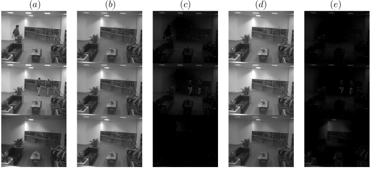
Figure S.13: Video surveillance with low-rank parameter $q=1$: (a) Original Frames. (b)-(c) Background extraction and outliers from robust regression conducted on adaptive capped least squares regression model. (d)-(e) Background extraction and outliers from the ordinary least squares method.

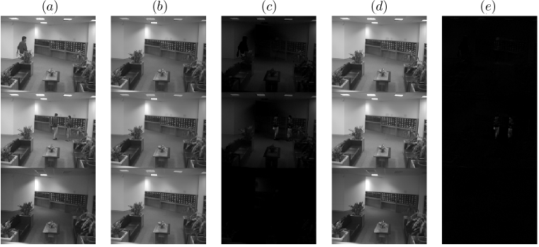
Figure S.14: Video surveillance with low-rank parameter $q=2$: (a) Original Frames. (b)-(c) Background extraction and outliers from robust regression conducted on adaptive capped least squares regression model. (d)-(e) Background extraction and outliers from the ordinary least squares method.

Figure S.15: Video surveillance with low-rank parameter $q=3$: (a) Original Frames. (b)-(c) Background extraction and outliers from robust regression conducted on adaptive capped least squares regression model. (d)-(e) Background extraction and outliers from the ordinary least squares method.

Appendix S.7 Blind Image Inpainting

We reformulate (6.2) as

$$\mathop{\mathrm{argmin}}_{\alpha\in\mathbb{R}^{m\times p},\{\delta_{i}\}_{i=1}^{p}} \sum_{i=1}^{p}\Bigg{(}\frac{1}{2}\|(y_{i}-D\alpha_{i})\odot(1_{n}-\delta_{i})\|_{2}^{2}+\lambda\|\alpha_{i}\|_{1}+\frac{1}{2}\tau^{2}\sum_{j=1}^{n}\delta_{ij}\Bigg{)},$$ (S.7.1)

s.t. $$\delta_{ij}=1(|y_{ij}-[D\alpha_{i}]_{j}|>\tau),\;i=1,...,p,j=1,...,n,$$

where $D$ is a dictionary matrix, $\lambda$ is the regularization parameter, $\delta_{i}=(\delta_{i1},\cdots,\delta_{in})^{\mathrm{\scriptscriptstyle T}}$, $\delta_{ij}$ is a decision variable taking values 0 or 1, $[D\alpha_{i}]_{j}$ is the $j$th element of $D\alpha_{i}$, and $\odot$ denotes the Hadamard product.

To solve (S.7.1), we develop an alternating minimization algorithm to iteratively update $\alpha$ and $\delta_{i}$ in the order of $\alpha\rightarrow\delta_{i}$. Let

$$f(\alpha,\Delta;Y,D,\lambda)=\frac{1}{2}\|(Y-D\alpha)\odot(1_{n}1_{p}^{\mathrm{\scriptscriptstyle T}}-\Delta)\|_{2,1}^{2}+\sum_{i=1}^{n}\lambda\|\alpha_{i}\|_{1},$$

where $\Delta=(\delta_{ij})$ and $\|\cdot\|_{2,1}^{2}$ is the $\ell_{1}$-norm of the row-wise $\ell_{2}$-norms. For a fixed $\Delta$, optimizing (S.7.1) with respect to $\alpha$ becomes

$$\mathop{\mathrm{argmin}}_{\alpha\in\mathbb{R}^{m\times p}}f(\alpha,\Delta;Y,D,\lambda).$$ (S.7.2)

For a fixed $\alpha$, we update $\delta_{ij}$ using the feasibility conditions $\delta_{ij}=1(|y_{ij}-[D\alpha_{i}]_{j}|>\tau),\,1\leq i\leq p,\,1\leq j\leq n$.

The full algorithm goes as follows. We initialize $\Delta^{0}=1_{n}1_{p}^{\mathrm{\scriptscriptstyle T}}$. At iteration $k\geq 0$, we first apply Lasso to update

$$\alpha^{k+1}=\mathop{\mathrm{argmin}}_{\alpha\in\mathbb{R}^{m\times p}}f(\alpha,\Delta^{k};Y,D,\lambda),$$

then we update $\delta^{k+1}_{ij}=1(|y_{ij}-[D\alpha^{k+1}_{i}]_{j}|>\tau)$ and repeat the above steps until convergence, that is, $\Delta^{k+1}=\Delta^{k}$. We use the output $Y\odot(1-\Delta^{k+1})+D\alpha^{k+1}\odot\Delta^{k+1}$ for the signal matrix restoration. Algorithm 3 summarizes the pseudo code.

Algorithm 3 An alternating minimization algorithm for blind image inpainting using CLS.

1:  Algorithm: $\{\widehat{\alpha},\widehat{\Delta}\}\leftarrow\text{CLS-inpainting}\big{(}Y,D,\tau)$

2:  Initialization: $\Delta^{0}=1_{n}1_{p}^{\mathrm{\scriptscriptstyle T}}$

3:  Input: $\tau>0,D,\lambda$

4:  for $k=0,1,\cdots,\textbf{until }\Delta^{k+1}=\Delta^{k}$ ${\bf do}$$\alpha^{k+1}=\mathop{\mathrm{argmin}}_{\alpha\in\mathbb{R}^{m\times p}}f(\alpha,\Delta^{k};Y,D,\lambda)$,$\delta_{ij}^{k+1}=1(|y_{ij}-[D\alpha^{k+1}_{i}]_{j}|>\tau)\;\text{for}\;i=1,\cdots p,j=1,\cdots n$.end for

5:  Output: $\{\widehat{\alpha},\widehat{\Delta}\}=\{\alpha^{k+1},\Delta^{k+1}\}$

References

- Adheesh et al. (2018) Adheesh, B., Yanyan, S., Namita, S., Erjie, X., Bishnu, G., Shixu, L. and Xiaohua, Z. (2018). MAL2 promotes proliferation, migration, and invasion through regulating epithelial-mesenchymal transition in breast cancer cell lines. Biochemical and Biophysical Research Communications 504 434–439.
- Bondell and Stefanski (2013) Bondell, H. D. and Stefanski, L. A. (2013). Efficient robust regression via two-stage generalized empirical likelihood. Journal of the American Statistical Association 108 644–655.
- Chernozhukov et al. (2014) Chernozhukov, V., Chetverikov, D. and Kato, K. (2014). Gaussian approximation of suprema of empirical processes. The Annals of Statistics 42 1564–1597.
- Donoho and Huber (1983) Donoho, D. L. and Huber, P. J. (1983). The notion of breakdown point. In A Festschrift for Erich L. Lehmann (P. J. Bickel, K. Doksum and J. L. Hodges, eds.). Belmont, Wadsworth, CA, 157–184.
- Du et al. (2018) Du, R., Liu, B., Zhou, L., Wang, D., He, X., Xu, X., Zhang, L., Niu, C. and Liu, S. (2018). Downregulation of annexin a3 inhibits tumor metastasis and decreases drug resistance in breast cancer. Cell Death & Disease 9 126.
- Fan et al. (2017) Fan, J., Li, Q. and Wang, Y. (2017). Estimation of high dimensional mean regression in the absence of symmetry and light tail assumptions. Journal of the Royal Statistical Society. Series B, Statistical methodology 79 247.
- Gervini and Yohai (2002) Gervini, D. and Yohai, V. J. (2002). A class of robust and fully efficient regression estimators. The Annals of Statistics 30 583–616.
- Griva et al. (2008) Griva, I., Nash, S. G. and Sofer, A. (2008). Linear and Nonlinear Optimization. Society for Industrial and Applied Mathematics, Philadelphia, USA.
- Hampel (1971) Hampel, F. R. (1971). A general qualitative definition of robustness. The Annals of Mathematical Statistics 42 1887–1896.
- He et al. (2000) He, X., Simpson, D. G. and Wang, G. (2000). Breakdown points of t-type regression estimators. Biometrika 87 675–687.
- Huber (1964) Huber, P. J. (1964). Robust estimation of a location parameter. The Annals of Mathematical Statistics 35 73–101.
- Huber (1973) Huber, P. J. (1973). Robust regression: asymptotics, conjectures and Monte Carlo. The Annals of Statistics 1 799–821.
- Li et al. (2004) Li, L., Huang, W., Gu, I. Y.-H. and Tian, Q. (2004). Statistical modeling of complex backgrounds for foreground object detection. IEEE Transactions on Image Processing 13 1459–1472.
- Mairal et al. (2009) Mairal, J., Bach, F., Ponce, J. and Sapiro, G. (2009). Online learning for matrix factorization and sparse coding. Journal of Machine Learning Research 11 19–60.
- Maronna et al. (2019) Maronna, R. A., Martin, R. D., Yohai, V. J. and Salibián-Barrera, M. (2019). Robust Statistics: Theory and Methods (with R). John Wiley & Sons, New York.
- Mili et al. (1996) Mili, L., Coakley, C. W. et al. (1996). Robust estimation in structured linear regression. The Annals of Statistics 24 2593–2607.
- Mizera and Müller (2002) Mizera, I. and Müller, C. H. (2002). Breakdown points of Cauchy regression-scale estimators. Statistics & Probability Letters 57 79–89.
- Müller (1995) Müller, C. H. (1995). Breakdown points for designed experiments. Journal of Statistical Planning and Inference 45 413–427.
- Nakata et al. (2004) Nakata, B., Takashima, T., Ogawa, Y., Ishikawa, T. and Hirakawa, K. (2004). Serum cyfra 21-1 (cytokeratin-19 fragments) is a useful tumour marker for detecting disease relapse and assessing treatment efficacy in breast cancer. British Journal of Cancer 91 873–878.
- Rousseeuw and Yohai (1984) Rousseeuw, P. and Yohai, V. (1984). Robust regression by means of S-estimators. In Robust and Nonlinear Time Series Analysis. Springer, 256–272.
- Rousseeuw (1984) Rousseeuw, P. J. (1984). Least median of squares regression. Journal of the American Statistical Association 79 871–880.
- Rousseeuw and Driessen (1999) Rousseeuw, P. J. and Driessen, K. V. (1999). A fast algorithm for the minimum covariance determinant estimator. Technometrics 41 212–223.
- Rousseeuw and Leroy (1987) Rousseeuw, P. J. and Leroy, A. M. (1987). Robust Regression and Outlier Detection. John Wiley & Sons, New York.
- Shangguan et al. (2012) Shangguan, L., Ti, X., Krause, U., Hai, B., Zhao, Y., Yang, Z. and Liu, F. (2012). Inhibition of tgf-/smad signaling by bambi blocks differentiation of human mesenchymal stem cells to carcinoma-associated fibroblasts and abolishes their protumor effects. Stem Cells 30 2810–2819.
- Simpson (1987) Simpson, D. G. (1987). Minimum hellinger distance estimation for the analysis of count data. Journal of the American statistical Association 82 802–807.
- Sun et al. (2020) Sun, Q., Zhou, W.-X. and Fan, J. (2020). Adaptive Huber regression. Journal of the American Statistical Association 115 254–265.
- van der Vaart and Wellner (1986) van der Vaart, A. and Wellner, J. (1986). Weak Convergence and Empirical Processes: with Applications to Statistics. Springer, New York.
- Wang et al. (2020) Wang, L., Peng, B., Bradic, J., Li, R. and Wu, Y. (2020). A tuning-free robust and efficient approach to high-dimensional regression. Journal of the American Statistical Association 1–44.
- Western (1995) Western, B. (1995). Concepts and suggestions for robust regression analysis. American Journal of Political Science 786–817.
- Wu et al. (2004) Wu, Z., Irizarry, R. A., Gentleman, R., Martinez-Murillo, F. and Spencer, F. (2004). A model-based background adjustment for oligonucleotide expression arrays. Journal of the American Statistical Association 99.
- Yohai (1987) Yohai, V. J. (1987). High breakdown-point and high efficiency robust estimates for regression. The Annals of Statistics 15 642–656.
- Yohai and Zamar (1988) Yohai, V. J. and Zamar, R. H. (1988). High breakdown-point estimates of regression by means of the minimization of an efficient scale. Journal of the American Statistical Association 83 406–413.