Super Twisting based Lyapunov Redesign for Uncertain Linear Delay Systems

Abstract

We present a new continuous Lyapunov Redesign (LR) methodology for the robust stabilization of a class of uncertain time-delay systems that is based on the so-called Super Twisting Algorithm. The main feature of the proposed approach is that allows one to simultaneously adjust the chattering effect and achieve asymptotic stabilization of the uncertain system, which is lost when continuous approximation of the unit control is considered. At the basis of the Super Twisting based LR methodology is a class of Lyapunov-Krasovskii functionals, whose particular form of its time derivative allows one to define a delay-free sliding manifold on which some class of smooth uncertainties are compensated.

I Problem statement

We consider uncertain linear time-delay system of the form

$$\begin{split}\dot{x}(t)&=\sum_{j=0}^{m}A_{j}x(t-h_{j})+B(u(t)+\delta(t,\bar{x})),\>t\geq 0,\\ x(t)&=\varphi(t),\>t\in[-h_{m},0],\end{split}$$ (1)

where the initial function $\varphi$ is considered to belong to the space of continuous functions, $x(t)\in\mathbb{R}^{n}$ is the state at present time, $A_{j}\in\mathbb{R}^{n\times n}$, $j=0,\ldots,m$, $B\in\mathbb{R}^{n\times k}$, the delays $0=h_{0}<h_{1}<\ldots<h_{m}$ are known, and the vector $\bar{x}^{T}(t):=\begin{pmatrix}x^{T}(t)&x^{T}(t-h_{1})&\ldots&x^{T}(t-h_{m})\end{pmatrix}$. The delayed state dependent uncertainty $\delta(t,\bar{x})$ is continuous in $\bar{x}$, for all $t\in\mathbb{R}$, and it is Lebesgue measurable in $t$, for all $\bar{x}\in\mathbb{R}^{(m+1)n}$. As specified by Assumption 3 in Section II, it is assumed that it can be divided into vanishing and non-vanishing terms. The non-vanishing terms in $\delta$ are assumed to be continuously differentiable in time. Moreover, its derivative and the vanishing terms are bounded by time dependent Lebesgue integrable functions (cf. with Chapter 3 in [1]).

Systems of the form (1) are pervasive in engineering [1], and design of robust control algorithms that mitigate the perturbation effects has been object of active research in the last decades [2, 3, 4, 5, 6]. As in systems without delays, Lyapunov redesign (LR) [7, 8, 9] methodology can be used to design a robust control law to stabilize time delay system (1) as long as two requirements are fulfilled [10, 11, 12, 13, 14]. The first one is the existence of a nominal control law that stabilizes the nominal system. This is, for system (1) with $\delta(t,\bar{x})=0$, there exist $K_{j}\in\mathbb{R}^{k\times n},\>j=0,\ldots,m,$ such that

$$u(t)=v_{nom}(t)=\sum_{j=0}^{m}K_{j}x(t-h_{j})$$ (2)

renders an asymptotical stable trivial solution of the closed-loop nominal system

$$\begin{split}\dot{x}(t)=&\sum_{j=0}^{m}G_{j}x(t-h_{j}),\>t\geq 0,\\ x(t)=&\varphi(t),\>t\in[-h_{m},0],\end{split}$$ (3)

where $G_{j}:=A_{j}+BK_{j}$ for $j=0,\ldots,m$. The second requirement is the existence of a Lyapunov-Krasovskii functional (or Lyapunov-Razumikhin function) such that it satisfies standard lower and upper bounds, and its time derivative along the solutions of the closed-loop system (3) is negative. In this paper, we consider the following well-known class of Lyapunov-Krasovskii functionals [15]

$$V(\varphi) =\varphi^{T}(0)P\varphi(0)+\sum_{j=1}^{m}\int_{-h_{j}}^{0}F_{j}\left(\vec{h},\theta,\varphi(\theta)\right)d\theta,$$ (4)

where $P\in\mathbb{R}^{n\times n}$ is a positive definite matrix, $\vec{h}:=\begin{pmatrix}h_{1},\ldots,h_{m}\end{pmatrix}$, and $F_{j}$ are continuous functions.

We condensate the above requirements in the LR methodology within the following assumption, which is regarded to be satisfied from now on:

Assumption 1

There exists a Lyapunov-Krasovskii functional of the form (4) such that for some $\alpha_{1},\>\alpha_{2},\>\alpha_{3}\in\mathbb{R}_{+}$

$$\alpha_{1}\|\varphi(0)\|^{2}\leq V(\varphi)\leq\alpha_{2}\|\varphi\|_{\mathcal{H}}^{2}$$ (5)

$$\left.\dot{V}(x_{t})\right\rvert_{\eqref{ec:sys_cl}}\leq-\alpha_{3}\|x(t)\|^{2},$$ (6)

where $\|\cdot\|_{\mathcal{H}}$ is introduced later on.

Classical LR. The LR consists in adjusting the control law $u(t)$ by adding a robustifying discontinuous controller $v(t)$ to the nominal one, i.e. $u(t)=v_{nom}(t)+v(t)$, such that $v(t)$ is capable of compensating the uncertainty within the time derivative of the Lyapunov-Krasovskii functional, while recovering the negative sign in its upper-bound. More specifically, notice that the time derivative of the functional $V$ along the solutions of uncertain system (1) yields

$$\begin{split}\left.\dot{V}(x_{t})\right\rvert_{\eqref{ec:linear_sys}}\leq-\alpha_{3}\|x(t)\|^{2}+2x^{T}(t)PB\left(v(t)+\delta(t,\bar{x})\right).\end{split}$$

By taking the unit control

$$v(t)=-\rho_{\delta}(t,\bar{x})\frac{2B^{T}Px(t)}{\|2B^{T}Px(t)\|},$$ (7)

where $\rho_{\delta}$ is a known function such that $\|\delta(t,\bar{x})\|\leq\rho_{\delta}(t,\bar{x})$, one obtains

$$2x^{T}(t)PB(v(t)+\delta(t,\bar{x}))\leq 0.$$ (8)

Thus, the negativeness of the time derivative of the functional is recovered and the asymptotic stability of system (1) is ensured (cf. Theorem 3.1. in [15]). The main drawback of this approach resides in the discontinuity of the control law (7) in a switching manifold of relative degree one, which produces the undesirable chattering effect.

Continuous LR. In order to make a continuous LR, a continuous approximation of the unit controller (7) can be considered [16]. Namely,

$$v(t)\!=\!\left\{\begin{matrix}-\rho_{\delta}(t,\bar{x})\frac{2B^{T}Px(t)}{\|2B^{T}Px(t)\|},\;\rho_{\delta}(t,\bar{x})\|{2B^{T}Px(t)}\|\geq\varepsilon,\\ -\rho_{\delta}^{2}(t,\bar{x})\frac{2B^{T}Px(t)}{\varepsilon},\;\rho_{\delta}(t,\bar{x})\|{2B^{T}Px(t)}\|<\varepsilon\end{matrix}\right.$$ (9)

where $\varepsilon$ is a given real positive number. However, with such an approximation it is not possible to recover a time derivative of $V$ with definite sign anymore. Indeed,

$$\begin{split}2x^{T}(t)PB(v(t)+\delta(t,\bar{x}))\leq-\rho_{\delta}^{2}\frac{\|2B^{T}Px(t)\|^{2}}{\varepsilon}+\|2B^{T}Px(t)\|\rho_{\delta}\leq\frac{\varepsilon}{4},\end{split}$$

and the perturbation within the time derivative of the functional is no longer compensated. The system’s solutions are restricted to an arbitrarily small neighborhood of the trivial solution in a sufficiently large time and, to maintain the solutions bounded in this region, extremely high gains of the controller are required. Thus, as one cannot ensure asymptotic stability of the uncertain system (1) anymore, the critical issue is the compromise between controller effort and the attainable residual set where the solutions will be contained. This approach was used with Lyapunov-Razumikhin functions in the early work [10], and similarly later appeared with Lyapunov-Krasovskii functionals in [11, 12] for the design of adaptive control algorithms.

Contribution. An open question of practical interest within LR methodology is whether it is possible to design a continuous controller that simultaneously makes system (1) asymptotically stable and adjusts the chattering effect, at least for systems with fast actuators [17]. In this paper, inspired by the ideas introduced in [18, 19], we look at the classical LR from a second order Sliding Mode Control (SMC) perspective by defining the sliding variable as

$$w(t):=2B^{T}Px(t)$$ (10)

and the sliding manifold by

$$\mathcal{S}:=\{x\in\mathbb{R}^{n}:w(t)=0\}.$$

We propose a continuous LR methodology that relies on the super twisting algorithm (STA), a well-known technique within the SMC framework that ensures a stable second order sliding mode on the manifold $\mathcal{S}$ [20, 21, 22, 23]. Since the discontinuous term is integrated in the STA, the control signal is absolutely continuous at the expense of theoretically exact compensation of smooth perturbations. By using the STA instead of any continuous approximation of unit control, we ensure the asymptotic stability of the trivial solution of the uncertain system (1), which is the premise of a classical LR. Moreover, STA does not require a boundary layer strategy as in (9) but a single robustifying controller does the task. Notice that, in contrast to the classical LR where one looks for inequality (8) to be satisfied, in the presented approach we restrict $x\in\mathcal{S}$.

It is important to mention that few research work addressing the robust stabilization of time-delay systems via STA has been reported in the literature, see for instance [24, 25]. The reported results there are within the standard SMC framework, where one requires a transformation of the delay system to a regular form and the design of a sliding manifold. Robust stabilization via the LR approach requires neither of both.

The note is organized as follows. The continuous LR methodology based on the STA is introduced in Section II. The theoretical results are illustrated with an example in Section III, and the paper ends with some final remarks in Section IV.

The following notation is adopted throughout the paper. The Euclidian norm for vectors and matrices is denoted by $\|\cdot\|$. The space of continuous functions defined on $[-h,0]$ with values in $\mathbb{R}^{n}$ is denoted by $C\left([-h,0],\mathbb{R}^{n}\right)$ and it is equipped with the supremum norm

$$\|\varphi\|_{\mathcal{H}}:=\sup_{\theta\in[-h,0]}\|\varphi(\theta)\|.$$

The notation $x_{t}$ represents the state function $x_{t}(\theta)=x(t+\theta)$, $\theta\in[-h_{m},0]$. The space of positive real numbers is represented by $\mathbb{R}_{+}$.

II Continuous Lyapunov redesign for TDS

We present the continuous LR methodology based on the STA. Let $w$ in (10) be defined as a sliding variable. We address the robust stabilization of system (1) by enforcing $w$ to be zero in finite time via a second order sliding mode controller and ensuring asymptotic convergence of the system’s solutions to the origin on the sliding manifold $\mathcal{S}$.

Let us assume

Assumption 2

$\operatorname{rank}B=k$.

Consider the control law in system (1) as

$$u(t)=v_{nom}(t)+v(t),$$ (11)

where

$$v(t)=-\left(2B^{T}PB\right)^{-1}(2B^{T}P\left(\sum_{j=0}^{m}G_{j}x(t-h_{j})\right)-u_{sta}(t)),$$ (12)

with $P\in\mathbb{R}^{n\times n}$ from functional (4), $u_{sta}$ denotes the STA of variable gains introduced in [21, 23] given by

$$\begin{split}u_{sta}(t)=&-k_{1}(t,\bar{x},\bar{\bar{x}})\xi_{1}(w)+\rho(t)\\ \dot{\rho}(t)=&-k_{2}(t,\bar{x},\bar{\bar{x}})\xi_{2}(w),\end{split}$$ (13)

where $k_{1}$, $k_{2}$ and $\bar{\bar{x}}$ are specified later on, $k_{3}$ is any positive real number and

$$\begin{split}\xi_{1}(w)&:=\dfrac{w(t)}{\|w(t)\|^{1/2}}+k_{3}w(t),\\ \xi_{2}(w)&:=\dfrac{w(t)}{2\|w(t)\|}+\frac{3k_{3}}{2}\dfrac{w(t)}{\|w(t)\|^{1/2}}+k_{3}^{2}w(t).\end{split}$$

By setting $k_{3}=0$ and lifting the dependence of gains $k_{1}$ and $k_{2}$ on the state and delays, one recovers the standard STA, which has been recently studied for a class of time-delay systems in [24, 25]. A remarkable difference is that here the sliding manifold is not designed but results from the Lyapunov-Krasovskii functional used for the stability analysis of the nominal system.

It is well-known that since the STA produces a continuous signal, it cannot compensate perturbations satisfying $\|\delta(t,\bar{x})\|\leq\rho_{\delta}(t,\bar{x})$ [20]. That is the reason why we introduce the following assumptions on the system uncertainty:

Assumption 3

The uncertainty term can be divided as

$$2B^{T}PB\delta(t,\bar{x})=d_{1}(t,x)+\delta_{z}(t,\bar{x}),$$ (14)

where $d_{1}(t,x)=0$ if $x\in\mathcal{S}$ and $\delta_{z}$ is such that

$$\frac{\partial\delta_{z}}{\partial x(t-h_{j})}B=0,\>j=0,\ldots,m.$$

Assumption 4

There exist known functions $\rho_{1}:\mathbb{R}_{+}\times\mathbb{R}^{n}\rightarrow\mathbb{R}_{+}$ and $\rho_{2}:\mathbb{R}_{+}\times\mathbb{R}^{(m+1)n}\times\mathbb{R}\rightarrow\mathbb{R}_{+}$ such that

$$\begin{split}\|d_{1}(t,x)\|\leq&\rho_{1}(t,x)\|\xi_{1}(w)\|,\\ \|d_{2}(t,\bar{x},\bar{\bar{x}})\|\leq&\rho_{2}(t,\bar{x},\bar{\bar{x}})\|\xi_{2}(w)\|,\end{split}$$

where

$$d_{2}(t,\bar{x},\bar{\bar{x}}):=\dot{\delta}_{z}(t,\bar{x})=\frac{\partial\delta_{z}}{\partial t}+\bar{\bar{x}}(t),$$

where $\bar{\bar{x}}(t):=\frac{\partial\delta_{z}}{\partial\bar{x}}\dot{\bar{x}}(t).$

Remark 1

Let $H_{h}$ denote the set of all possible sums of pairs of delays $(h_{i},h_{j})$, $i,j=0,\ldots,m$, the vector $\bar{\bar{x}}$ depends on terms of the form $x(t-h_{\kappa})$ with $h_{\kappa}\in H_{h}$. For example, for two delays $h_{1}$ and $h_{2}$, $H_{h}=\left\{h_{0},h_{1},h_{2},2h_{1},2h_{2},h_{1}+h_{2}\right\}$ and $\bar{\bar{x}}$ depends on $x(t),x(t-h_{1}),x(t-h_{2}),x(t-2h_{1}),x(t-2h_{2}),x(t-h_{1}-h_{2}).$

It is important to mention that whereas the component $d_{1}$ contains terms that vanish while $x\in\mathcal{S}$ for $t\geq T>0$, the component $d_{2}$ contains non-vanishing terms including those that are delay dependent, i.e. terms of the form $x(t-h_{i})$, $i=1,\ldots,m$. These terms do not vanish until $t\geq T+h_{m}$.

Let us consider the following Lyapunov function, used in the proof of Proposition 1 in the Appendix (cf. with [21, 23]),

$$V_{st}(w,z)=\gamma^{T}P_{st}\gamma,$$

where

$$\gamma:=\begin{pmatrix}\xi_{1}(w)\\ z\end{pmatrix},\>P_{st}:=\begin{pmatrix}\left(\beta+4\epsilon^{2}\right)I&-2\epsilon I\\ -2\epsilon I&I\end{pmatrix},$$

and set the gains of the STA in (13) as

$$\begin{split}&k_{1}(t,\bar{x},\bar{\bar{x}})=\delta+\frac{1}{\beta}\left(\frac{1}{4\epsilon}\left(4\epsilon\rho_{1}+\rho_{2}\right)^{2}+2\epsilon\rho_{2}+\epsilon+(2\epsilon+\rho_{1})\left(\beta+4\epsilon^{2}\right)\right),\\ &k_{2}(t,\bar{x},\bar{\bar{x}})=\beta+4\epsilon^{2}+2\epsilon k_{1}(t,\bar{x},\bar{\bar{x}}),\end{split}$$ (15)

where $\delta,\>\beta,\>\epsilon\in\mathbb{R}_{+}$. In the next theorem we state the main result of the paper, i.e. the robust stabilization of system (1) by control (11).

Theorem 1

Suppose Assumptions 1, 2, 3 and 4 are satisfied. Trajectories of closed-loop system (1), (11), with $v_{nom}$ and $v$ given by (2) and (12) respectively, reach the sliding manifold $\mathcal{S}$ in finite time

$$T=\dfrac{2}{\eta_{2}}\ln\left(1+\dfrac{\eta_{2}}{\eta_{1}}\sqrt{V_{st}(w_{0},z_{0})}\right),$$

with

$$\eta_{1}=\frac{\epsilon\sqrt{\lambda_{\min}(P_{st})}}{\lambda_{\max}(P_{st})},\>\eta_{2}=\frac{2\epsilon k_{3}}{\lambda_{\max}(P_{st})},$$

and after that they asymptotically converge to the origin.

Proof 1

The proof is splitted into two parts. First, it is proved that with robust controller (11) the trajectories of system (1) converge to the sliding manifold $\mathcal{S}$ in finite time, and then that they asymptotically converge to the origin.

From Assumption 3 it follows that

$$\delta(t,\bar{x})=\frac{1}{2}\left(B^{T}PB\right)^{-1}\left(d_{1}(t,x)+\delta_{z}(t,\bar{x})\right),$$

hence, differentiating $w$ along the solutions of system (1), (11), yields

$$\dot{w}(t)=u_{sta}(t)+d_{1}(t,x)+\delta_{z}(t,\bar{x}).$$ (16)

By taking the change of variable $z(t):=\rho(t)+\delta_{z}(t,\bar{x})$, where $\rho$ is from the STA (13), we arrive at

$$\begin{split}\dot{w}(t)=&-k_{1}(t,\bar{x},\bar{\bar{x}})\xi_{1}(w)+z(t)+d_{1}(t,x),\\ \dot{z}(t)=&-k_{2}(t,\bar{x},\bar{\bar{x}})\xi_{2}(w)+d_{2}(t,\bar{x},\bar{\bar{x}}).\end{split}$$ (17)

By Proposition 1 in Appendix, system (17) with gains given by (15) is finite time stable.

Now, notice that closed-loop system (1), (11) is

$$\begin{split}\dot{x}(t)=E\sum_{j=0}^{m}G_{j}x(t-h_{j})+\frac{1}{2}B(B^{T}PB)^{-1}u_{sta}+B\delta(t,\bar{x}),\end{split}$$

where $E=I-B(B^{T}PB)^{-1}B^{T}P$. It follows from equation (16) that

$$\begin{split}\dot{x}(t)=E\sum_{j=0}^{m}G_{j}x(t-h_{j})+\frac{1}{2}B(B^{T}PB)^{-1}\dot{w}(t).\end{split}$$

Thus, on the sliding manifold $\mathcal{S}$,

$$\begin{split}\dot{x}(t)=E\sum_{j=0}^{m}G_{j}x(t-h_{j}),\>\>x\in\mathcal{S}.\end{split}$$ (18)

In order to prove that the trajectories asymptotically converge to the origin, let us consider a Lyapunov-Krasovskii functional $V$ of the form (4) satisfying conditions of Assumption 1. The derivative of $V$ along the solutions of system (18) satisfies

$$\begin{split}\left.\dot{V}(x_{t})\right\rvert_{\eqref{ec:reduced_system}}&\leq-\alpha_{3}\|x(t)\|^{2}-2x^{T}(t)PB(B^{T}PB)^{-1}B^{T}PE\sum_{j=0}^{m}G_{j}x(t-h_{j})\\ &=-\alpha_{3}\|x(t)\|^{2}-w^{T}(t)(B^{T}PB)^{-1}B^{T}PE\sum_{j=0}^{m}G_{j}x(t-h_{j})\\ &=-\alpha_{3}\|x(t)\|^{2},\>x\in\mathcal{S}.\end{split}$$

This proves the asymptotic stability of system (18), and in turn completes the proof.

The methodology for the design of robust controller is summarized as follows:

1. Propose a Lyapunov-Krasovskii functional of the form (4) that satisfy the conditions of Assumption 1.

2. Select the sliding variable $w(t)=2B^{T}Px(t)$, where matrix $P$ is from the Lyapunov-Krasovskii functional proposed in Step 1.

3. Find $\rho_{1}$ and $\rho_{2}$ satisfying Assumption 4.

4. Select controller $v(t)$ as (12) with a given sliding variable $w(t)$ in Step 2.

5. Fix the gains as in (15) with upper-bounds given in Step 3.

III Example

The obtained results are illustrated with an example. The performance of the unit control (7), continuous approximation (9) and the STA (13) are compared. It is worth mentioning that the considered system cannot be robustly stabilized by the approach proposed in [11, 12].

Example 1

We consider a system of the form (1) with $h_{1}=h=2$ and matrices [29]

$$A_{0}=\begin{pmatrix}2&0\\ 1.75&0.25\end{pmatrix},\>A_{1}=\begin{pmatrix}-1&0\\ -0.1&-0.25\end{pmatrix},\>B=\begin{pmatrix}1\\ 1\end{pmatrix}.$$

For the sake of simulation, consider the uncertainty term as

$$\delta(t,x)=\dfrac{1}{3}\left(\sin(t)+2(x_{1}(t-h)-x_{2}(t-h))\right).$$

Notice that the associated nominal system is not stabilizing by a memoryless feedback since the pair $(A_{0},B)$ is not controllable. The robust stabilization of this system has been addressed in [29] via SMC. We next present the simulation results obtained with control

$$u(t)=v_{nom}(t)+v(t),$$

where $v(t)$ is considered to be of three classes: unit control of the form (7), continuous control with approximation (9) with $\varepsilon=0.05$, and continuous control based on STA (13). In all of them we consider the same nominal control and the same associated Lyapunov-Krasovskii functional of the form (4):

$$V(x_{t})=x^{T}(t)Px(t)+\int_{-h}^{0}\left(x^{T}(t+\xi)Qx(t+\xi)d\xi+\int_{\theta-h}^{0}x^{T}(t+\xi)Rx(t+\xi)d\xi\right)d\theta$$

where

$$P =\begin{pmatrix}2.8063&0.8062\\ 0.8062&0.6559\end{pmatrix},\>Q=\begin{pmatrix}9.1429&3.3997\\ 3.3997&1.3327\end{pmatrix},$$

$$R =\begin{pmatrix}4.6439&1.5632\\ 1.5632&0.6352\end{pmatrix}.$$

Stabilizing gains of the nominal system are found to be

$$K_{1}=\begin{pmatrix}-3.7648&-0.73\end{pmatrix},\>K_{2}=\begin{pmatrix}1.1964&0.1723\end{pmatrix}.$$

The sliding variable is

$$w(t)=2B^{T}Px(t)=7.2251x_{1}(t)+2.9244x_{2}(t).$$

Let us define $c=\frac{2}{3}B^{T}PB=3.3832$ and consider the gain $k_{3}=0$. The uncertainty satisfies Assumption 3 with $d_{1}(t,x)=0$ and

$$\delta_{z}(t,\bar{x})=c\left(\sin(t)+2(x_{1}(t-h)-x_{2}(t-h))\right).$$

It is clear that $\dfrac{\partial\delta_{z}}{\partial x(t-h)}B=0$. Then, the uncertainty also satisfies Assumption 4 with $\rho_{1}(t,x)=0$ and,

$$\rho_{2}(t,\bar{x},\bar{\bar{x}})=(4c^{2}\left(1+2|0.5x_{2}(t-2h)-1.8x_{1}(t-2h)|^{2}\right)+2c^{2}|x_{1}(t-h)-x_{2}(t-h)|^{2})^{1/2}.$$

For unit control (7) and continuous approximation (9), consider $\rho_{\delta}(t,\bar{x})=\frac{1}{3}(1+2|x_{1}(t-h)-x_{2}(t-h)|)$.

Set then the gains $k_{1}$ and $k_{2}$ as in (15) with the parameters

$$\delta=1.5,\>\beta=1,\>\epsilon=0.3.$$

Figure 1 depicts the norm of the closed-loop solution. One observes that the LR based on STA has a better performance in comparison with the continuous approximation (9) and the unit control (7). Indeed, closed-loop solution of the system with (9) does not converge to the origin but it is restricted to a small neighborhood. Figure 2 shows the control laws, where the reduction of chattering with respect to the unit control is clearly visualized.

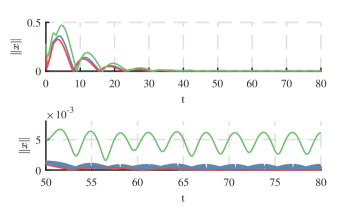
Figure 1: Top: Norm of the closed-loop solution obtained with LR based on unit control (blue), continuous LR based on approximation (9) (green), and LR based on STA (red). Bottom: Simulation result of the last 30 seconds

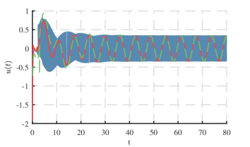
Figure 2: Top: Control signals of LR based on LR based on unit control (blue), continuous LR based on approximation (9) (green), and LR based on STA (red). Bottom: Simulation result of the last 30 seconds.

IV Conclusions

The robust stabilization of a class of uncertain systems with delays via a new continuous LR methodology based on the STA was addressed. A remarkable feature of the proposed approach is that it allows one to ensure asymptotic stability of the system using continuous control signals.

As a direct consequence of the considered class of Lyapunov-Krasovskii functionals, the associated sliding variable is delay-free. The latter allowed us to combine the STA with the LR technique without eliminating the sliding modes (see Chapter 13 in [30] and Section IV in [31]), providing a flexible, robust design methodology that can be easily extended to more complex scenarios studied in SMC for delay-free systems.

Appendix A Proposition 1

Proposition 1

Under Assumptions 1, 2, 3 and 4, system

$$\begin{split}\dot{w}(t)=&-k_{1}(t,\bar{x},\bar{\bar{x}})\xi_{1}(w)+z(t)+d_{1}(t,x),\\ \dot{z}(t)=&-k_{2}(t,\bar{x},\bar{\bar{x}})\xi_{2}(w)+d_{2}(t,\bar{x},\bar{\bar{x}}),\end{split}$$

with $k_{1}$ and $k_{2}$ given by (15), is finite time stable with

$$T=\dfrac{2}{\eta_{2}}\ln\left(1+\dfrac{\eta_{2}}{\eta_{1}}\sqrt{V_{st}(w_{0},z_{0})}\right).$$

Proof 2

The proof follows the same arguments as those presented in [23] up to the dependence of the gains on the delayed states. Let us consider the Lyapunov function

$$V_{st}(w,z)=\gamma^{T}P_{st}\gamma,$$

where

$$\gamma=\gamma(w,z):=\begin{pmatrix}\xi_{1}(w)\\ z\end{pmatrix},\>P_{st}:=\begin{pmatrix}\left(\beta+4\epsilon^{2}\right)I&-2\epsilon I\\ -2\epsilon I&I\end{pmatrix}.$$

The Lyapunov function $V_{st}$ is differentiable everywhere except on the set $\mathcal{W}:=\{(w,z)\in\mathbb{R}^{2k}:w=0\}$. Let us define $\xi_{1}^{\prime}(w):=\dfrac{d}{dw}\xi_{1}(w)\in\mathbb{R}^{k\times k}$. We observe that

$$\begin{split}\xi_{1}^{\prime}(w)=&\|w\|^{-1/2}I-\dfrac{1}{2}ww^{T}\|w\|^{-5/2}+k_{3}I\\ =&\frac{1}{\|w\|^{1/2}}\left(I-\frac{1}{2}\frac{ww^{T}}{\|w\|^{2}}\right)+k_{3}I\end{split}$$

for any different from zero $w\in\mathbb{R}^{k}$. We recall from [23] some properties of that are useful throughout the proof:

1. $\xi_{2}(w)=\xi_{1}^{\prime}(w)\xi_{1}(w),\>\>\forall w\neq 0$.

2. Matrix $\xi_{1}^{\prime}(w)$ is symmetric and positive definite for any different from zero $w\in\mathbb{R}^{k}$. Moreover,

   $$\lambda_{\min}(\xi_{1}^{\prime}(w))\|y\|^{2}\leq y^{T}\xi_{1}^{\prime}(w)y,\>\>\forall y\in\mathbb{R}^{k},$$

   with $\lambda_{\min}(\xi_{1}^{\prime}(w))=\dfrac{1}{2\|w\|^{1/2}}+k_{3}$.

3. $\|\xi_{1}^{\prime}(w)\|=\dfrac{1}{\|w\|^{1/2}}+k_{3}.$

By Property 1,

$$\begin{split}\dot{\gamma}=\begin{pmatrix}\xi_{1}^{\prime}(w)\dot{w}\\ \dot{z}\end{pmatrix}&=\begin{pmatrix}\xi_{1}^{\prime}(w)\left(-k_{1}\xi_{1}(w)+z+d_{1}\right)\\ -k_{2}\xi_{1}^{\prime}(w)\xi_{1}(w)+d_{2}\end{pmatrix}\\ &=A_{st}\gamma+f,\>(w,z)\in\mathbb{R}^{2k}\setminus\mathcal{W},\end{split}$$

where

$$A_{st}=A_{st}(t,\bar{x},\bar{\bar{x}}):=\begin{pmatrix}-k_{1}(t,\bar{x},\bar{\bar{x}})\xi_{1}^{\prime}(w)&\xi_{1}^{\prime}(w)\\ -k_{2}(t,\bar{x},\bar{\bar{x}})\xi_{1}^{\prime}(w)&0\end{pmatrix}$$

and

$$f=f(t,\bar{x},\bar{\bar{x}}):=\begin{pmatrix}d_{1}(t,x)\\ d_{2}(t,\bar{x},\bar{\bar{x}}))\end{pmatrix}.$$

Hence,

$$\dfrac{d}{dt}V_{st}(w,z)=-\gamma^{T}Q\gamma+2\gamma^{T}P_{st}f.$$

where

$$Q_{st} :=-\left(P_{st}A_{st}+A_{st}^{T}P_{st}\right)$$

$$=\begin{pmatrix}2\beta k_{1}-4\epsilon\left(\beta+4\epsilon^{2}\right)\xi_{1}^{\prime}(w)&0\\ 0&4\epsilon\xi_{1}^{\prime}(w)\end{pmatrix}.$$

From Assumption 4, it follows that

$$\begin{split}\gamma^{T}P_{st}f\leq&(\beta+4\epsilon^{2})\|\xi_{1}^{T}\xi_{1}^{\prime}(w)\|\|d_{1}\|+2\epsilon\|z\|\|\xi_{1}^{\prime}(w)\|\|d_{1}\|+\left(2\epsilon\|\xi_{1}\|+\|z\|\right)\|d_{2}\|\\ \leq&(\beta+4\epsilon^{2})\|\xi_{1}^{T}\xi_{1}^{\prime}(w)\|\rho_{1}\|\xi_{1}\|+2\epsilon\|z\|\|\xi_{1}^{\prime}(w)\|\rho_{1}\|\xi_{1}\|+\left(2\epsilon\|\xi_{1}\|+\|z\|\right)\rho_{2}\|\xi_{2}\|.\end{split}$$

Then, from equality $\|\xi_{1}^{T}\xi_{1}^{\prime}\|=\lambda_{\min}(\xi_{1}^{\prime}(w))\|\xi_{1}\|$ and $2\|\xi_{1}^{\prime}(w)\|\leq 4\lambda_{\min}(\xi_{1}^{\prime}(w))$, we obtain

$$2\gamma^{T}P_{st}f\leq 2\lambda_{\min}(\xi_{1}^{\prime}(w))((\beta+4\epsilon^{2})\|\xi_{1}\|^{2}\rho_{1}+4\epsilon\|z\|\|\xi_{1}\|\rho_{1}+2\epsilon\|\xi_{1}\|^{2}\rho_{2}+\|z\|\|\xi_{1}\|\rho_{2}),$$ (19)

and from Property 2 we have that for any $\gamma\in\mathbb{R}^{2k}$

$$-\gamma^{T}Q_{st}\gamma\leq-\lambda_{\min}(\xi_{1}^{\prime}(w))\left(\left(2\beta k_{1}-4\epsilon\left(\beta+4\epsilon^{2}\right)\right)\|\xi_{1}\|^{2}+4\epsilon\|z\|^{2}\right).$$ (20)

By (20) and (19),

$$\dfrac{d}{dt}V_{st}(w,z)\leq-\lambda_{\min}(\xi_{1}^{\prime}(w))\hat{\gamma}^{T}\hat{Q}\hat{\gamma},$$

with $\hat{\gamma}:=\begin{pmatrix}\|\xi_{1}\|&\|z\|\end{pmatrix}^{T}$ and

$$\hat{Q}=\begin{pmatrix}2\beta k_{1}-(4\epsilon+2\rho_{1})(\beta+4\epsilon^{2})-4\epsilon\rho_{2}&-4\epsilon\rho_{1}-\rho_{2}\\ \star&4\epsilon\end{pmatrix}.$$

Considering $k_{1}$ as in (15) one has that $\hat{Q}-2\epsilon I>0$, hence

$$\dfrac{d}{dt}V_{st}(w,z)\leq-2\epsilon\lambda_{\min}(\xi^{\prime}(w))\|\hat{\gamma}\|^{2}.$$

Since $\|w\|^{1/2}\leq\|\xi_{1}\|\leq\|\hat{\gamma}\|$ and $\lambda_{\min}(P_{st})\|\hat{\gamma}\|^{2}\leq V_{st}(w,z)\leq\lambda_{\max}(P_{st})\|\hat{\gamma}\|^{2}$,

$$\begin{split}\dfrac{d}{dt}V_{st}(w,z)&\leq-2\epsilon\left(\frac{1}{2\|w\|^{1/2}}+k_{3}\right)\|\hat{\gamma}\|^{2}\\ &\leq-\eta_{1}\sqrt{V_{st}(w,z)}-\eta_{2}V_{st}(w,z),\end{split}$$

where

$$\eta_{1}=\frac{\epsilon\sqrt{\lambda_{\min}(P_{st})}}{\lambda_{\max}(P_{st})},\>\eta_{2}=\frac{2\epsilon k_{3}}{\lambda_{\max}(P_{st})}.$$

Finally, as the solution of the differential equation

$$\dot{v}_{c}(t)=-\eta_{1}\sqrt{v_{c}(t)}-\eta_{2}v_{c}(t),\>v_{c}(0):=v_{c_{0}}$$

is determined by

$$v_{c}(t)=e^{-\eta_{2}t}\left(v_{c_{0}}^{1/2}+\dfrac{\eta_{1}}{\eta_{2}}\left(1-e^{\frac{{\eta_{2}}}{2}t}\right)\right)^{2}$$

it follows from the comparison theorem that $(w,z)$ converges to zero in finite time

$$T=\dfrac{2}{\eta_{2}}\ln\left(1+\dfrac{\eta_{2}}{\eta_{1}}\sqrt{V_{st}(w_{0},z_{0})}\right).$$

References

• [1] V. Kolmanovskii and A. Myshkis, Introduction to the theory and applications of functional differential equations.   Dordrecht: Springer Science + Business Media, 1999.
• [2] J.-P. Richard, F. Gouaisbaut, and W. Perruquetti, “Sliding mode control in the presence of delay,” Kybernetika, vol. 37, no. 3, pp. 277–294, 2001.
• [3] X. Han, E. Fridman, S. K. Spurgeon, and C. Edwards, “On the design of sliding-mode static-output-feedback controllers for systems with state delay,” IEEE Transactions on Industrial Electronics, vol. 56, no. 9, pp. 3656–3664, 2009.
• [4] X. Han, E. Fridman, and S. K. Spurgeon, “Sliding-mode control of uncertain systems in the presence of unmatched disturbances with applications,” International Journal of Control, vol. 83, no. 12, pp. 2413–2426, 2010.
• [5] T. R. Oliveira, J. P. V. Cunha, and A. Battistel, “Global stability and simultaneous compensation of state and output delays for nonlinear systems via output-feedback sliding mode control,” Journal of Control, Automation and Electrical Systems, vol. 27, no. 6, pp. 608–620, 2016.
• [6] T. Sanchez, A. Polyakov, J.-P. Richard, and D. Efimov, “Sliding-mode stabilization of SISO bilinear systems with delays,” in Variable-Structure Systems and Sliding-Mode Control.   Springer, 2020, pp. 215–236.
• [7] S. Gutman, “Uncertain dynamical systems–A Lyapunov min-max approach,” IEEE Transactions on Automatic Control, vol. 24, no. 3, pp. 437–443, 1979.
• [8] G. Leitmann, “Guaranteed asymptotic stability for some linear systems with bounded uncertainties,” Journal of Dynamic Systems Measurement and Control- Transactions of the ASME, vol. 101, no. 3, pp. 212–216, 1979.
• [9] H. K. Khalil, Nonlinear systems.   Macmillan Publishing Company, 1992.
• [10] A. Thowsen, “Uniform ultimate boundedness of the solutions of uncertain dynamic delay systems with state-dependent and memoryless feedback control,” International Journal of control, vol. 37, no. 5, pp. 1135–1143, 1983.
• [11] H. Wu, “Adaptive robust tracking and model following of uncertain dynamical systems with multiple time delays,” IEEE Transactions on Automatic Control, vol. 49, no. 4, pp. 611–616, 2004.
• [12] ——, “Adaptive robust control of uncertain nonlinear systems with nonlinear delayed state perturbations,” Automatica, vol. 45, no. 8, pp. 1979–1984, 2009.
• [13] L. Rodríguez-Guerrero, S. Mondié, and O. Santos-Sánchez, “Guaranteed cost control using Lyapunov redesign for uncertain linear time delay systems,” IFAC-PapersOnLine, vol. 48, no. 12, pp. 392–397, 2015.
• [14] L. Rodríguez-Guerrero, C. Cuvas-Castillo, O.-J. Santos-Sánchez, J.-P. Ordaz-Oliver, and C.-A. García-Samperio, “Robust guaranteed cost control for a class of perturbed systems with multiple distributed time delays,” Journal of Process Control, vol. 80, pp. 127–142, 2019.
• [15] E. Fridman, Introduction to time-delay systems: Analysis and control.   Springer, 2014.
• [16] E. Ryan and M. Corless, “Ultimate boundedness and asymptotic stability of a class of uncertain dynamical systems via continuous and discontinuous feedback control,” IMA journal of mathematical control and information, vol. 1, no. 3, pp. 223–242, 1984.
• [17] U. Pérez-Ventura and L. Fridman, “When is it reasonable to implement the discontinuous sliding-mode controllers instead of the continuous ones? frequency domain criteria,” International Journal of Robust and Nonlinear Control, vol. 29, no. 3, pp. 810–828, 2019.
• [18] S. V. Drakunov, W.-C. Su, and Ü. Özgüner, “Constructing discontinuity surfaces for variable structure systems: A Lyapunov approach,” Automatica, vol. 32, no. 6, pp. 925–928, 1996.
• [19] M. A. Estrada, L. Fridman, and J. Moreno, “Control of fully actuated mechanical systems via super-twisting based Lyapunov redesign,” in Proceedings of the IFAC World Congress, 2020, pp. 5192–5195.
• [20] A. Levant, “Sliding order and sliding accuracy in sliding mode control,” International journal of control, vol. 58, no. 6, pp. 1247–1263, 1993.
• [21] J. A. Moreno, “Lyapunov approach for analysis and design of second order sliding mode algorithms,” in Sliding Modes after the first decade of the 21st Century.   Springer, 2011, pp. 113–149.
• [22] J. A. Moreno and M. Osorio, “Strict lyapunov functions for the super-twisting algorithm,” IEEE Transactions on Automatic Control, vol. 57, no. 4, pp. 1035–1040, 2012.
• [23] P. V. Vidal, E. V. Nunes, and L. Hsu, “Output-feedback multivariable global variable gain super-twisting algorithm,” IEEE Transactions on Automatic Control, vol. 62, no. 6, pp. 2999–3005, 2016.
• [24] L. F. R. Jerónimo, J. Z. Torres, B. Saldivar, J. Dávila, and J. C. Á. Vilchis, “Robust stabilisation of linear time-invariant time-delay systems via first order and super-twisting sliding mode controllers,” IET Control Theory & Applications, vol. 14, no. 1, pp. 175–186, 2019.
• [25] H. Caballero-Barragán, L. P. Osuna-Ibarra, A. G. Loukianov, and F. Plestan, “Sliding mode predictive control of linear uncertain systems with delays,” Automatica, vol. 94, pp. 409–415, 2018.
• [26] S.-I. Niculescu and W. Michiels, “Stabilizing a chain of integrators using multiple delays,” IEEE Transactions on Automatic Control, vol. 49, no. 5, pp. 802–807, 2004.
• [27] W. Michiels, S.-I. Niculescu, and L. Moreau, “Using delays and time-varying gains to improve the static output feedback stabilizability of linear systems: a comparison,” IMA Journal of Mathematical Control and Information, vol. 21, no. 4, pp. 393–418, 2004.
• [28] E. Fridman and L. Shaikhet, “Delay-induced stability of vector second-order systems via simple lyapunov functionals,” Automatica, vol. 74, pp. 288–296, 2016.
• [29] F. Gouaisbaut, M. Dambrine, and J.-P. Richard, “Robust control of delay systems: a sliding mode control design via LMI,” Systems & control letters, vol. 46, no. 4, pp. 219–230, 2002.
• [30] W. Perruquetti and J.-P. Barbot, Sliding mode control in engineering.   Marcel Dekker, 2002.
• [31] D. Efimov and A. Aleksandrov, “Analysis of robustness of homogeneous systems with time delays using Lyapunov-Krasovskii functionals,” Int J of Robust and Nonlinear Control, pp. 1–17, 2020, https://doi.org/10.1002/rnc.5115.