Inverse Design of Grating Couplers Using the Policy Gradient Method from Reinforcement Learning

Abstract

We present a proof-of-concept technique for the inverse design of electromagnetic devices motivated by the policy gradient method in reinforcement learning, named PHORCED (PHotonic Optimization using REINFORCE Criteria for Enhanced Design). This technique uses a probabilistic generative neural network interfaced with an electromagnetic solver to assist in the design of photonic devices, such as grating couplers. We show that PHORCED obtains better performing grating coupler designs than local gradient-based inverse design via the adjoint method, while potentially providing faster convergence over competing state-of-the-art generative methods. As a further example of the benefits of this method, we implement transfer learning with PHORCED, demonstrating that a neural network trained to optimize 8^∘ grating couplers can then be re-trained on grating couplers with alternate scattering angles while requiring >$10\times$ fewer simulations than control cases.

Keywords adjoint method; deep learning; integrated photonics; inverse design; optimization; reinforcement learning

1 Introduction

There has been a recent, massive surge in research syncretizing topics in photonics and artificial intelligence / machine learning (AI/ML), including photonic analog accelerators [1, 2, 3, 4, 5, 6, 7, 8], physics emulators [9, 10, 11, 12, 13, 14, 15], and AI/ML-enhanced inverse electromagnetic design techniques [16, 17, 18, 19, 20, 21, 22, 23, 24, 25, 26, 27, 28, 29, 30, 31, 32, 15, 33, 34, 35]. While inverse electromagnetic design via local gradient-based optimization with the adjoint method has been successfully applied to a multitude of design problems throughout the entirety of the optics and photonics communities [36, 37, 38, 39, 40, 41, 42, 43, 44, 45, 46, 47, 48, 49, 50, 51, 52, 53, 54, 55, 56, 57, 58, 59, 60], inverse electromagnetic design leveraging AI/ML techniques promise superior computational performance, advanced data analysis and insight, or improved effort towards global optimization. For the lattermost topic in particular, Jiang and Fan recently introduced an unsupervised learning technique called GLOnet which uses a generative neural network interfaced with an electromagnetic solver to design photonic devices such as metasurfaces and distributed Bragg reflectors [24, 25, 26]. In this paper we propose a conceptually similar design technique, but with a contrasting theoretical implementation motivated by a concept in reinforcement learning called the policy gradient method – specifically a one-step implementation of the REINFORCE algorithm [61, 62]. We will refer to our technique as PHORCED = PHotonic Optimization using REINFORCE Criteria for Enhanced Design. PHORCED is compatible with any external physics solver including EMopt [63], a versatile electromagnetic optimization package that is employed in this work to perform 2D simulations of single-polarization grating couplers.

In Section 2, we will qualitatively compare and contrast three optimization techniques: local gradient-based optimization (e.g., gradient ascent), GLOnet, and PHORCED. We are specifically interested in a proof-of-concept demonstration of the PHORCED optimization technique applied to grating couplers, which we present in Section 3. We find that both our implementation of the GLOnet method and PHORCED find better grating coupler designs than local gradient-based optimization, but PHORCED requires fewer electromagnetic simulation evaluations than GLOnet. Finally, in Section 4 we introduce the concept of transfer learning to integrated photonic optimization, where in our application we demonstrate that a neural network trained to design 8^∘ grating couplers with the PHORCED method can be re-trained to design grating couplers that scatter at alternate angles with greatly accelerated time-to-convergence. We speculate that a hierarchical optimization protocol leveraging this technique can be used to design computationally complex devices while minimizing computational overhead.

2 Extending the Adjoint Method with Neural Networks

Local gradient-based optimization using the adjoint method has been successfully applied to the design of a plethora of electromagnetic devices. Detailed tutorials of the adjoint method applied to electromagnetic optimization may be found in Refs. [36, 37, 38, 39, 43, 46, 60]. Here, we qualitatively illustrate a conventional design loop utilizing the adjoint method in Fig. 1(a). This begins with the choice of an initial electromagnetic structure parameterized by vector $\mathbf{p}$, which might represent geometrical degrees-of-freedom like the width and height of the device. This is fed into an electromagnetic solver, denoted by a function $g$. The resulting electric and magnetic fields, $\mathbf{x}=g(\mathbf{p})$, can be used to evaluate a user-defined electromagnetic merit function $f(\mathbf{x})$ – the metric that we are interested in optimizing (e.g., coupling efficiency). Gradient-based optimization seeks to improve the value of the merit function by updating the design parameters, $\mathbf{p}$, in a direction specified by the gradient of the electromagnetic merit function, $\frac{\partial(f\circ g)}{\partial\mathbf{p}}$. The value of the gradient may be obtained very efficiently using the adjoint method, requiring just two electromagnetic simulations regardless of the number of degrees-of-freedom (called the forward simulation and adjoint simulation, respectively). A single iteration of gradient-based optimization is depicted visually in the center of Fig. 1(a), where $p$ is a single-dimension point sampled along a toy merit function $(f\circ g)(p)$ representing the optimization landscape (which is unknown, a priori). The derivative (gradient) of the merit function is illustrated by the arrow pointing from $p$ in the direction of steepest ascent (assuming this is a maximization problem). During an optimization, we slowly update $p$ in this direction until a local optimum is reached.

The adjoint method chain-rule derivative of the electromagnetic merit function resembles the concept of backpropagation in deep learning, where a neural network’s weights can be updated efficiently by application of the chain-rule with information from the forward pass. Naturally, we might extend the functionality of the adjoint method by placing a neural network in the design loop. The neural network takes the place of a deterministic update algorithm (such as gradient ascent), potentially learning information or patterns in the design problem that allows it to find a better optimum. Below we present two methods to implement inverse design with neural networks: GLOnet (introduced by Jiang and Fan [24, 25]) and PHORCED (this work). Both methods are qualitatively similar, but differ in the representation of the neural network. In the main text of this manuscript we will qualitatively describe the differences between these techniques; a detailed mathematical discussion may be found in Supplementary Material Section 1.

The GLOnet optimization method is depicted qualitatively in Fig. 1(b). The neural network is represented as a deterministic function $h_{\boldsymbol{\theta}}$ that takes in noise $\mathbf{z}$ from some known distribution D and outputs design parameters $\mathbf{p}$. Importantly, the neural network is parameterized by programmable weights $\boldsymbol{\theta}$ that we intend to optimize in order to generate progressively better electromagnetic devices. Similar to regular gradient ascent, we may evaluate the electromagnetic merit function of a device generated by the neural network $(f\circ g)(\mathbf{p})$ using our physics solver, and find its gradient with respect to the design parameters using the adjoint method, $\frac{\partial(f\circ g)}{\partial\mathbf{p}}$. However, the GLOnet design problem is inherently stochastic because of the presence of noise, and therefore the optimization objective becomes the expected value of the electromagnetic merit function, $\operatorname*{\mathbb{E}}_{\mathbf{z}}[(f\circ g\circ h_{\boldsymbol{\theta}})(\mathbf{z})]$ – sometimes called the reward in the reinforcement learning literature . In practice this expression can be approximated by taking a simple average over the electromagnetic merit functions of several devices generated by the neural network per iteration. The gradient that is then backpropagated to the neural network is given by the expected value of the chain-rule gradient of the reward function. The first term, $\frac{\partial(f\circ g)}{\partial\mathbf{p}}$, can once again be computed very efficiently using the adjoint method, requiring just two electromagnetic simulations per device. Meanwhile the latter term, $\frac{\partial\mathbf{p}}{\partial\boldsymbol{\theta}}|_{\mathbf{p}=h_{\mathbf{\theta}}(\mathbf{z})}$, can be calculated internal to the neural network using conventional backpropagation with automatic differentiation. Visually, one iteration of the GLOnet method is shown in the center of Fig. 1(b). In each iteration, the neural network in the GLOnet method suggests parameters, $p_{i}$, which are then individually simulated. Similar to gradient-based optimization from Fig. 1(a), we find the gradient of the merit function value with respect to each generated design parameter, represented by the arrows pointing towards the direction of steepest ascent at each point. The net gradient information from many simulated devices effectively tells the neural network where to explore in the next iteration. With a dense search, the global optimum along the domain of interest can potentially be found.

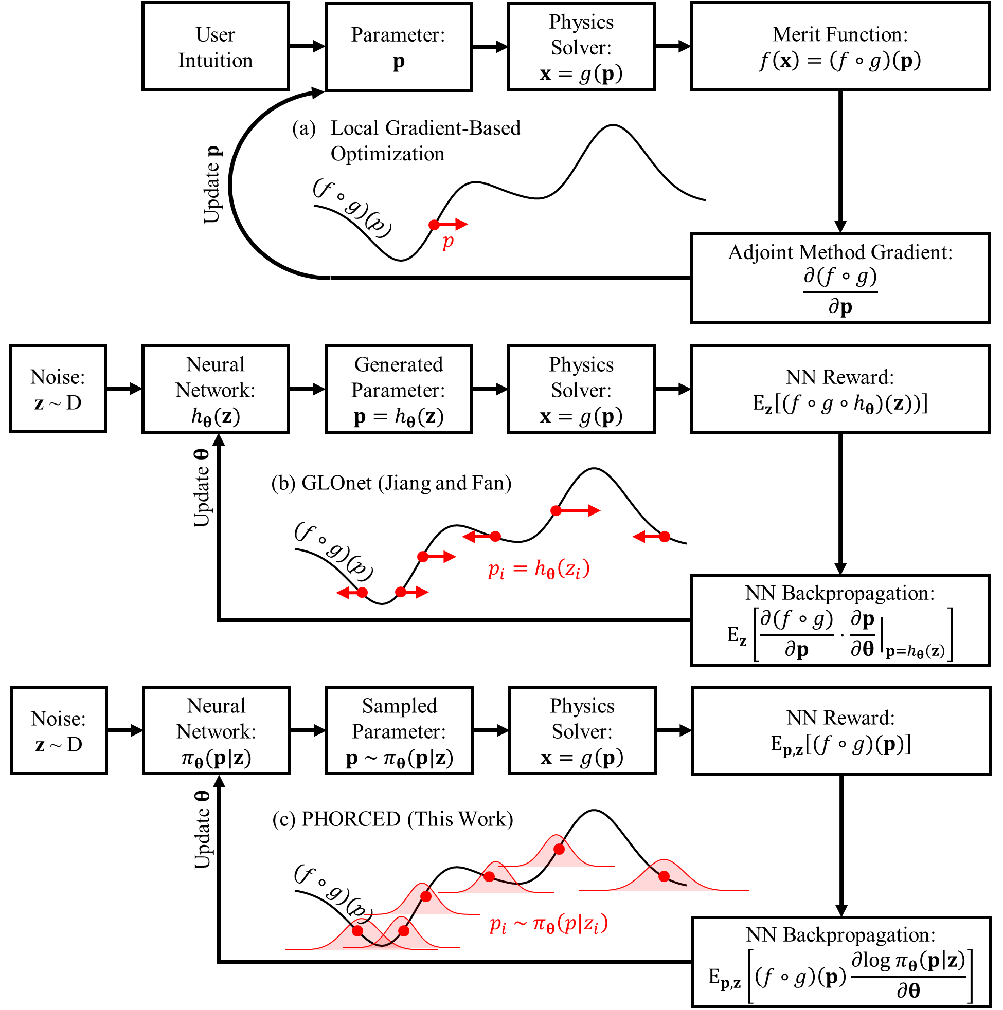
Figure 1: Neural networks provide a natural extension to conventional inverse design via the adjoint method. A typical gradient-based design loop is shown in (a) where the derivatives are calculated using the adjoint method. The GLOnet method (b), originally proposed by Jiang and Fan [24, 25], replaces a conventional gradient-based optimization algorithm with a deterministic neural network. In this work we propose PHORCED (c), which uses a probabilistic neural network to generate devices. (b) and (c) are qualitatively similar, but require different gradients in backpropagation because of the representation of the neural network (deterministic versus probabilistic). In particular, notice that PHORCED does not require an evaluation of the adjoint method gradient of the electromagnetic merit function, $\frac{\partial(f\circ g)}{\partial\mathbf{p}}$.

Our technique, called PHORCED, is provided in Fig. 1(c). Qualitatively speaking, it is very similar to GLOnet, but is motivated differently from a mathematical perspective. PHORCED is a special case of the REINFORCE algorithm [61, 62] from the field of reinforcement learning (RL), applied to electromagnetic inverse design. In particular, the neural network is treated as purely probabilistic, defining a continuous conditional probability density function over parameter variables $\mathbf{p}$ conditioned on the input vector $\mathbf{z}$ – denoted by $\pi_{\boldsymbol{\theta}}(\mathbf{p}|\mathbf{z})$. In other words, instead of outputting $\mathbf{p}$ deterministically given input noise, the neural network outputs probabilities of generating $\mathbf{p}$. We then randomly sample a parameter vector $\mathbf{p}$ for simulation and evaluation of the reward. Note that $\pi_{\boldsymbol{\theta}}(\mathbf{p}|\mathbf{z})$ is called the policy in RL, and in this work is chosen to be a multivariate Gaussian distribution with mean vector and standard deviation of random variable $\mathbf{p}$ as outputs. The reward for PHORCED is qualitatively the same as GLOnet – namely, we intend to optimize the expected value of the electromagnetic merit function. However, because both $\mathbf{p}$ and $\mathbf{z}$ are random variables, we take the joint expected value: $\operatorname*{\mathbb{E}}_{\mathbf{p},\mathbf{z}}[(f\circ g)(\mathbf{p})]$. Furthermore, because of the probabilistic representation of the neural network, the gradient of the reward with respect to the neural net weights for backpropagation is much different than the corresponding GLOnet case. In particular, we find that the backpropagated chain-rule gradient requires no evaluation of the gradient of the electromagnetic merit function, $\frac{\partial(f\circ g)}{\partial\mathbf{p}}$. Consequently, the electromagnetic adjoint simulation is no longer required, implying that fewer simulations are required overall for PHORCED compared to GLOnet under equivalent choices of neural network architecture and hyperparameters . PHORCED is visually illustrated in the center of Fig. 1(c). The neural network defines Gaussian probability density functions conditioned on input noise vectors $z_{i}$, shown in the light red bell curves representing $\pi_{\mathbf{\theta}}(p|z_{i})$, from which we sample points $p_{i}$ to simulate Using information from the merit function values, the neural network learns to update the mean and standard deviation of the Gaussians. Consequently, we emphasize that the Gaussian policy distribution is not static because its statistical parameters are adjusted by the trainable weights of the neural network, and is therefore capable of exploring throughout the feasible design space. For adequate choice of distribution and dense enough search, the PHORCED method can potentially find the global optimum in the domain of interest.

Before proceeding it should be remarked that the algorithms implemented by GLOnet and PHORCED have precedent in the literature, with some distinctions that we will outline here. Optimization algorithms similar to GLOnet were suggested in Refs. [64, 65], where the main algorithmic difference appears in the definition of the reward function. In particular, the reward defined in Ref. [64] was the same generalized form that we have presented in Fig. 1(b), while Jiang and Fan emphasized the use of an exponentially-weighted reward to enhance global optimization efforts [25]. On the other hand, PHORCED was motivated as a special case of the REINFORCE algorithm [61, 62], but also resembles some versions of evolutionary strategy [66, 67, 64, 65]. The main difference between PHORCED and evolutionary strategy (ignoring several heuristics) is the explicit use of a neural network to model the multivariate Gaussian policy distribution, albeit some recent works have used neural networks in their implementations of evolutionary strategy [67, 65] for different applications than those studied here. Furthermore, PHORCED does not require a Gaussian policy; any explicitly-defined probability distribution can be used as an alternative if desired. Beyond evolutionary strategy, a recent work in fluid dynamics [68] uses an algorithm akin to PHORCED called One-Step Proximal Policy Optimization (PPO-1) – a version of REINFORCE with a single policy, $\pi_{\boldsymbol{\theta}}$, operating on parallel instances of the optimization problem. The main distinction between PPO-1 and PHORCED is that we have implemented the option to use an input noise vector $\mathbf{z}$ to condition the output policy distribution, $\pi_{\boldsymbol{\theta}}(\mathbf{x}|\mathbf{z})$, which can effectively instantiate multiple distinct policies acting on parallel instances of the optimization problem. This potentially enables multi-modal exploration of the parameter space, bypassing a known issue of Bayesian optimization with Gaussian probability distributions [65]. However, note that the best results for the applications studied in this work used a constant input vector $\mathbf{z}$, thus making our implementation similar to PPO-1 in the results below. Regardless of the intricacies mentioned above, we emphasize that both GLOnet and PHORCED are unique in their application to electromagnetic optimization, to the authors’ knowledge. In the next section we will compare all three algorithms from Fig. 1 applied to grating coupler optimization.

3 Proof-of-Concept Grating Coupler Optimization

A grating coupler is a passive photonic device that is capable of efficiently diffracting light from an on-chip waveguide to an external optical fiber. Recent works have leveraged inverse design techniques in the engineering of grating couplers, resulting in state-of-the-art characteristics [44, 42, 52, 56, 21]. In this section we will show how generative neural networks can aid in the design of ultra-efficient grating couplers.

The grating coupler geometry used for our proof-of-concept is depicted in Fig. 2(a). We assume a silicon-on-insulator (SOI) wafer platform with a $280\,\mathrm{nm}$-thick silicon waveguide separated from the silicon substrate by a 2µm buried oxide (BOX) layer. The grating coupler consists of periodically spaced corrugations to the input silicon waveguide with etch depth $190\,\mathrm{nm}$. These grating coupler dimensions are characteristic of a high-efficiency integrated photonics platform operating in the C-band ($1550\,\mathrm{nm}$ central wavelength) as suggested by a transfer matrix based directionality calculation [55, 69], and are provided as an example in the open-source electromagnetic optimization package EMopt [63] that was used to perform forward and adjoint simulations in this work.

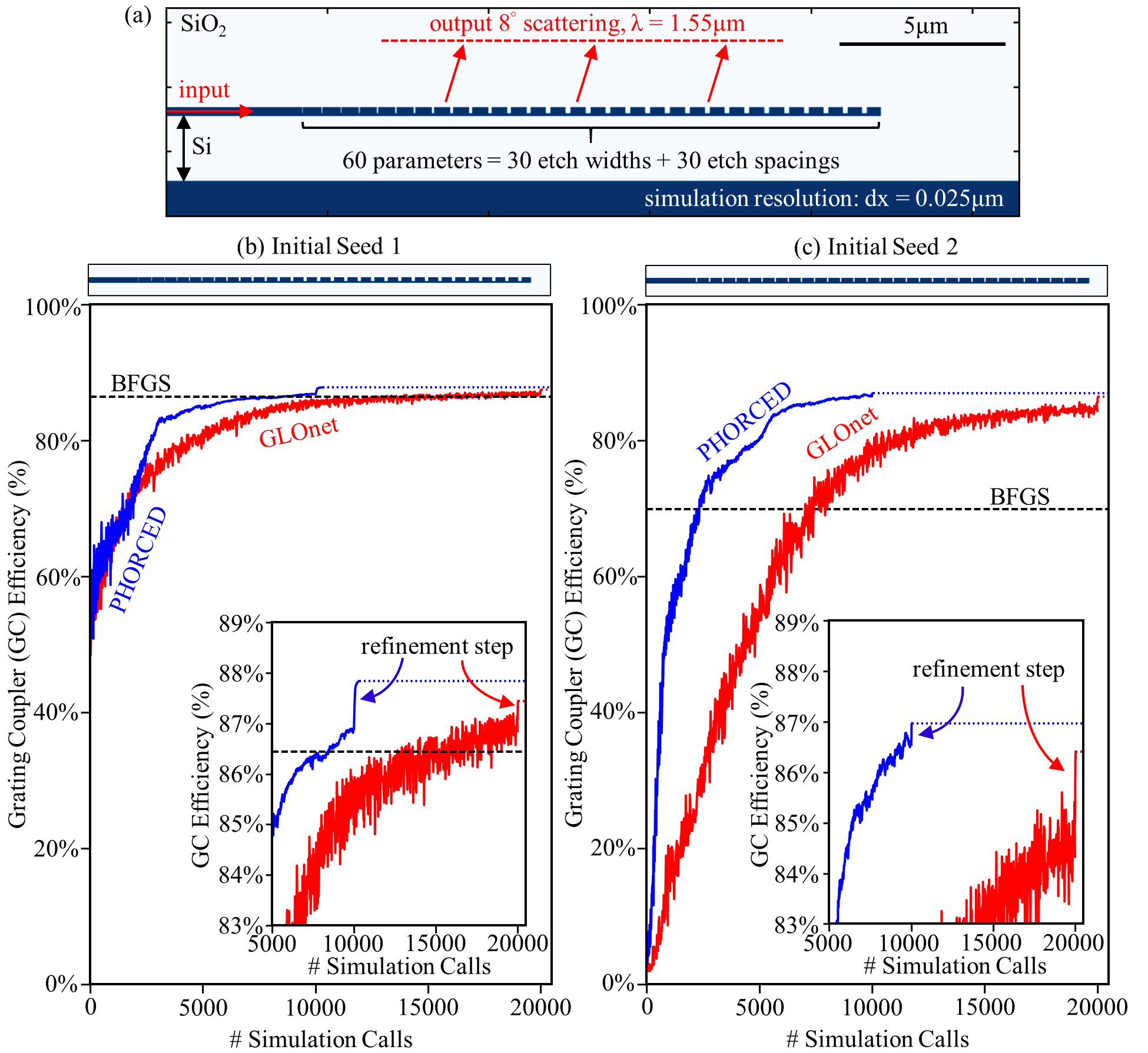
Figure 2: PHORCED and GLOnet outperform conventional gradient-based optimization, with different simulation evaluation requirements. The grating coupler simulation geometry for optimization is shown in (a), consisting of a SOI wafer platform with 280nm waveguide, 190nm etch depth, and 2µm BOX height. We optimized 60 device parameters in total, namely the width and spacing between 30 etch corrugations. The results of the BFGS, GLOnet, and PHORCED algorithms applied to Initial Seed 1 and Initial Seed 2 are presented in (b) and (c) as a function of the number of simulation calls. The initial seeds (grating designs) are illustrated above each optimization plot. The insets depict zoomed-in views of the peak efficiencies attained by PHORCED and GLOnet, along with respective BFGS refinement steps performed on the best design generated by each algorithm.

For our optimizations, we will consider 60 total designable parameters that define the grating coupler: the width of and spacing between 30 waveguide corrugations. For a well-designed grating coupler, input light to the waveguide scatters at some angle relative to vertical toward an external optical fiber. In this work we choose to optimize the grating coupler at fixed wavelength and scattering angle assuming specific manufacturing and assembly requirements for a modular optical transceiver application [70, 52]. In our case, the merit function for optimization is the coupling efficiency of scattered light with wavelength $\lambda=1550\,\text{nm}$ propagating $8^{\circ}$ relative to normal, mode-matched to an output Gaussian beam mode field diameter 10.4µm – characteristic of a typical optical fiber mode. The explicit definition of this electromagnetic merit function may be found in Refs. [44, 52, 71]. Note that we did not include fabrication constraints nor other specifications of interest in grating couplers in our parameterization choice, e.g. the BOX thickness and the Si etch depth, which will be desirable in future optimizations of experimentally-viable devices. Furthermore, the simulation domain is discretized with a $dx=25\text{nm}$ grid step which may result in some inaccuracy for very fine grating coupler features. This simulation discretization was chosen for feasibility of the optimization since individual simulations require about 4 seconds to compute on a high-performance server with over 30 concurrent MPI processes, and as we will show GLOnet and PHORCED can require as many as 20,000 simulation evaluations for convergence. Nevertheless, we utilized permittivity smoothing [43] to minimize the severity of this effect and obtain physically meaningful results.

We apply the Broyden–Fletcher–Goldfarb–Shanno (BFGS), GLOnet, and PHORCED algorithms to grating coupler optimization with two different initial designs (Initial Seed 1 and Initial Seed 2) in Fig. 2(b) and Fig 2(c). Initial Seed 1 corresponds to the grating depicted in Fig. 2(a) and the top of Fig. 2(b), where we used a parameter sweep to choose a linear apodization of the etch duty cycle before optimization. Initial Seed 2 corresponds to the grating shown at the top of Fig. 2(c) where we use a uniform duty cycle of 90%. Both initial designs have pitch that satisfy the grating equation [44, 52] for $8^{\circ}$ scattering. These initial seeds serve to explore the robustness of the optimization algorithms to “good” and “poor” choices of initial condition. Indeed, Initial Seed 1 satisfies physical intuition for a good grating coupler, because chirping the duty cycle is well-known to improve Gaussian beam mode-matching, and thus the initial grating coupler efficiency is already a reasonable value of 56%. Meanwhile, Initial Seed 2 has the correct pitch for $8^{\circ}$ scattering, but has a low efficiency of 1% owing to poor mode-matching and directionality. In essence, we are using these two cases as a proxy to explore whether PHORCED and GLOnet can reliably boost electromagnetic performance in a high-dimensional parameter space, even in cases where the intuition about the optimal initial conditions is limited.

BFGS is a conventional gradient-based optimization algorithm similar to that depicted in Fig. 1(a), and implemented using default settings from the open-source SciPy optimize module. After optimization with BFGS, the final simulated grating coupler efficiency of Initial Seed 1 and Initial Seed 2 are 86.4% and 69.9% respectively, which are shown in the black dashed lines of Fig. 2(b) and Fig. 2(c). Note that the number of simulation calls for BFGS is not shown because it is vastly smaller than that required for GLOnet and PHORCED (144 and 214 total simulations for Initial Seed 1 and Initial Seed 2, respectively).

The implementation of GLOnet and PHORCED for the grating coupler optimizations in Fig. 2(b) and Fig. 2(c) are described below; other details and specifications, such as a graphical illustration of the neural network models used in either case, may be found in Supplementary Materials Section 2. GLOnet is described qualitatively in Fig. 1(b) where we use a deterministic neural network and an exponentially-weighted electromagnetic merit function originally recommended by Jiang and Fan [24, 25] with a chosen hyperparameter $\sigma=0.6$. PHORCED is described qualitatively in Fig. 1(c) where we use a probabilistic neural network modeling a multivariate, isotropic Gaussian output distribution. The electromagnetic merit function used in the reward is just the unweighted grating coupler efficiency, except we used a “baseline” subtraction of the average merit function value in the backpropagated gradient (which is a common tactic in reinforcement learning for reducing model variance [72]). In both methods, we use a stopping criterion of 1,000 total optimizer iterations, with 10 devices sampled per iteration. Note that because GLOnet requires an adjoint simulation for each device and PHORCED does not, the effective stopping criteria are $1000\times 10\times 2=20,000$ simulation calls for GLOnet and $1000\times 10\times 1=10,000$ simulation calls for PHORCED. The neural network models for GLOnet and PHORCED were implemented in PyTorch, and are illustrated in Fig. S1 of the Supplementary Material. For GLOnet, we used a convolutional neural network with ReLU activations and linear output of the design vector. For PHORCED, we used a simple fully-connected neural network with ReLU activations and linear output defining the statistical parameters (mean and variance) of the Gaussian policy distribution. We applied initial conditions by adding the design vector representing Initial Seed 1 and Initial Seed 2 to either the direct neural network output or the mean of the Gaussian distribution for GLOnet and PHORCED, respectively. Hyperparameters such as the number of weights and learning rate of the neural network optimizer were individually tuned for GLOnet and PHORCED (specifications can be found in Fig. S2 of the Supplemental Material). For both neural networks, we used an input vector $\mathbf{z}$ of dimension 5. However, for GLOnet $\mathbf{z}$ was drawn from a uniform distribution $\mathcal{U}(-1,1)$, while for PHORCED we used a simple Dirac delta distribution centered on 1. In other words, the input for PHORCED was a constant vector of 1’s. In this work we achieved our best results with this choice, but similar results (within 1% absolute grating coupler efficiency) could be attained with alternative choices of input distribution. Anecdotally, we found that using a noisy input could improve training stability and performance in toy problems studied outside of this work, but further investigation is required.

We find that PHORCED and GLOnet outperform regular BFGS for both initial conditions studied in Fig 2. For Initial Seed 1 (Fig. 2(b)), we generated optimized grating coupler efficiencies of 86.9% and 87.2% for PHORCED and GLOnet, respectively. For Initial Seed 2 (Fig. 2(c)) we find optimized grating coupler efficiencies of 86.8% and 85.6% for PHORCED and GLOnet, respectively. Furthermore, as shown in the insets of Fig. 2(b) and Fig. 2(c), we were able to marginally improve each of the results by applying a BFGS “refinement step” to the best performing design output from GLOnet and PHORCED. This refinement step was limited to a maximum of 200 iterations, or until another default convergence criterion was met. For Initial Seed 1 we obtained improvements of $\{86.9\%\rightarrow 87.8\%\}$/$\{87.2\%\rightarrow 87.4\%$) for PHORCED/GLOnet, respectively. For Initial Seed 2, we find improvements of $\{86.8\%\rightarrow 87.0\%\}$/ $\{85.6\%\rightarrow 86.4\%\}$ for PHORCED/GLOnet, respectively. Since PHORCED and GLOnet are inherently statistical and noisy, the refinement step is useful for finding the nearest optimum without requiring one to run an exhaustive search of the neural network generator in inference mode,.

In summary, we find that the PHORCED + BFGS refinement optimization achieved the best performance for both Initial Seed 1 and Initial Seed 2 with final grating coupler efficiency of 87.8% and 87.0%, respectively. These results agree with a transfer matrix based directionality analysis of these grating coupler dimensions [55, 69], where we find that approximately 88% grating efficiency is possible under perfect mode-matching conditions – meaning that our result for Initial Seed 1 is close to a theoretical global optimum. Notably, GLOnet had better performance than PHORCED in Initial Seed 1 before the refinement step was applied, and it is possible that better results could have been achieved with further iterations of both algorithms (as indicated by the slowly rising slopes of the optimization curves in the insets of Fig. 2(b)-(c)). However, we emphasize that PHORCED required approximately $2\times$ fewer simulation than GLOnet with the same number of optimization iterations because of the lack of adjoint gradient calculations.

Perhaps the most important result of these optimizations is that both PHORCED and GLOnet proved to be resilient against our choice of initial condition. Indeed, while BFGS provided a competitive result for Initial Seed 1, it failed to find a favorable local optimum given Initial Seed 2. PHORCED and GLOnet, on the other hand, attained final results within 1% absolute grating coupler efficiency for both initial conditions. This outcome is promising when considering the relative sparsity of each algorithm’s search in a high-dimensional design space. Indeed, as mentioned previously, we only sampled 10 devices per iteration of the optimization, meaning that there were fewer samples than dimension of the resulting parameter vectors (60). As an additional reference, we compared our results to CMA-ES (implemented with the open-source package pycma), a popular “blackbox” global optimization algorithm that is known to be effective for high-dimensional optimization [66]. Under the same number of simulation calls as PHORCED (10,000), CMA-ES reached efficiencies of 87.3% and 86.7% for Initial Seed 1 and Initial Seed 2, respectively. Therefore our implementations of PHORCED and GLOnet are competitive with current state-of-the-art blackbox algorithms. While the simulation requirements for convergence of PHORCED and GLOnet remain computationally prohibitive for more complex electromagnetic structures than those studied here, in contrast to local gradient-based search, our results offer the possibility of global optimization effort in electromagnetic design problems, where we are capable of limiting the tradeoff of performance with search density as well as the need for human intervention in situations where physical intuition is more difficult to ascertain. Furthermore, we believe that our implementations of GLOnet and PHORCED have significant room for improvement, and have advantages that go beyond alternative global optimization algorithms like CMA-ES. In particular, leveraging advanced concepts in deep learning and reinforcement learning can further improve computational efficiency and performance. For example, whereas our implementations of PHORCED and GLOnet used simple neural networks, a ResNet architecture can improve neural network generalizability while simultaneously reducing overfitting [27]. Moreover, one could take advantage of complementary deep learning and reinforcement learning based approaches such as importance sampling [65, 72], or “model-based” methods that could utilize an electromagnetic surrogate model or inverse model to reduce the number of full electromagnetic Maxwell simulations needed for training [13, 28, 32, 19]. Alternatively, whereas we optimized our grating for a single objective (single wavelength, $8^{\circ}$ scattering) Jiang and Fan showed that generative neural network based optimization can be extremely efficient for multi-objective design problems (e.g., multiple wavelengths and scattering angles in metasurfaces [24]). Along the same vein, in the next section we will show how a technique known as transfer learning can be used to re-purpose a neural network trained with PHORCED for an alternative objective, meanwhile boosting computational efficiency and electromagnetic performance dramatically.

4 Transfer Learning with the PHORCED Method

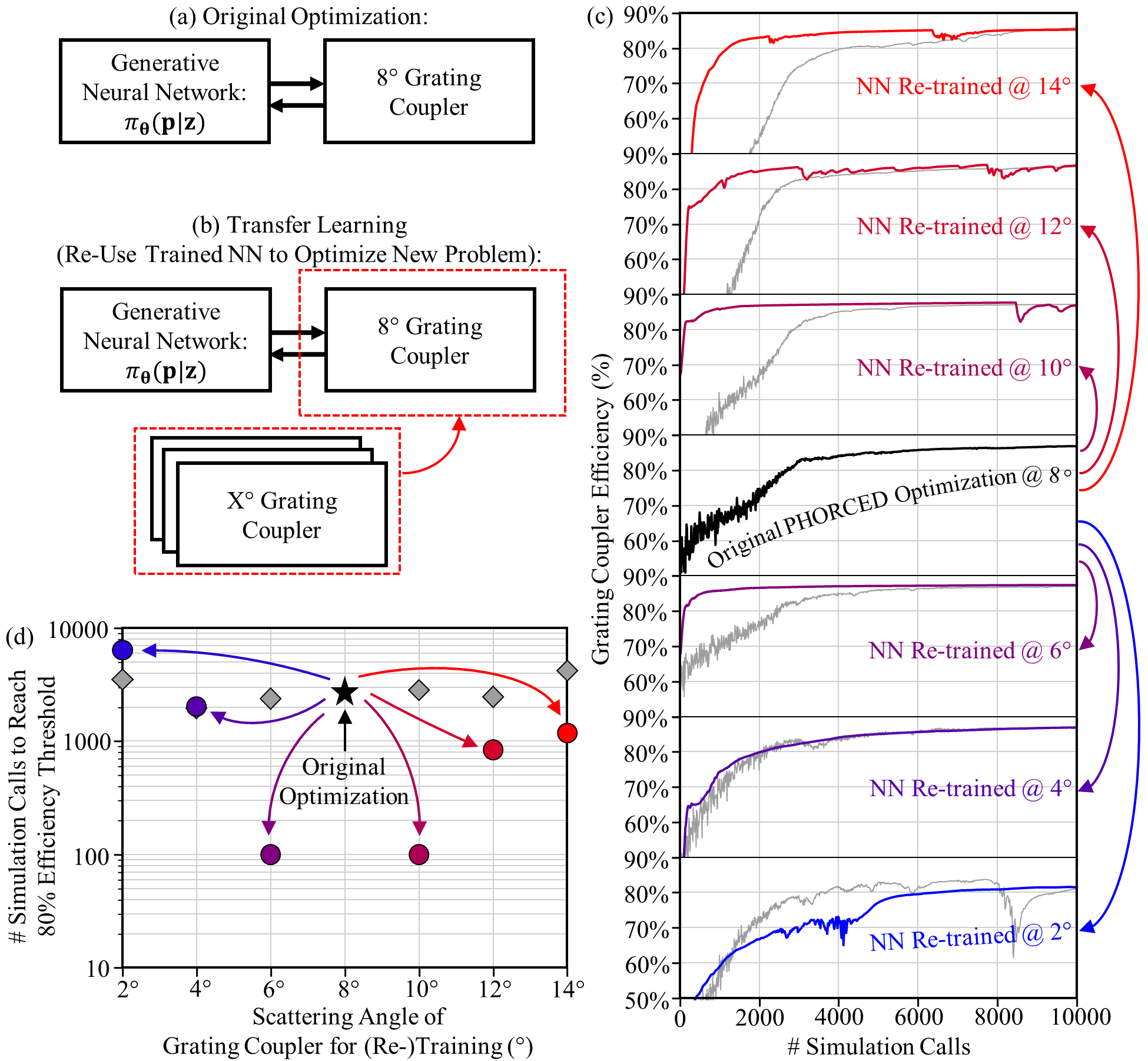
Figure 3: Transfer learning applied to grating coupler design yields accelerated convergence rate in optimization. The original PHORCED optimization from Fig. 2(b) is qualitatively depicted as a block diagram in (a) for comparison with the transfer learning approach in (b). Here, we exchange the $8^{\circ}$ grating coupler merit function with an alternative grating coupler angle for re-training. Optimization progressions as a function of the number of simulation calls for each of the re-training sessions are shown in the blue/red curves of (c). Control optimizations where transfer learning was not applied are plotted in gray for comparison. In (d) we plot the number of simulation calls for each optimization from (c) to reach 80% grating coupler scattering efficiency, with blue/red colored arrows and dots indicating applications of transfer learning and gray diamonds indicating the control cases.

Transfer learning is a concept in machine learning encompassing any method that reuses a model (e.g. a neural network) trained on one task for a different but related task. Qualitatively speaking and verified by real-world applications, we might expect the re-training of a neural network to occur faster than training a new model from scratch. Transfer learning has been extensively applied in classical machine learning tasks such as classification and regression, but has only recently been mentioned in the optics/photonics research domains [17, 27, 28, 33]. In this work we apply transfer learning to the inverse design of integrated photonics for the first time (to the authors’ knowledge), revealing that a neural network trained using PHORCED for the design of $8^{\circ}$ grating couplers can be re-trained to design grating couplers with varied scattering angle and increased rate of convergence.

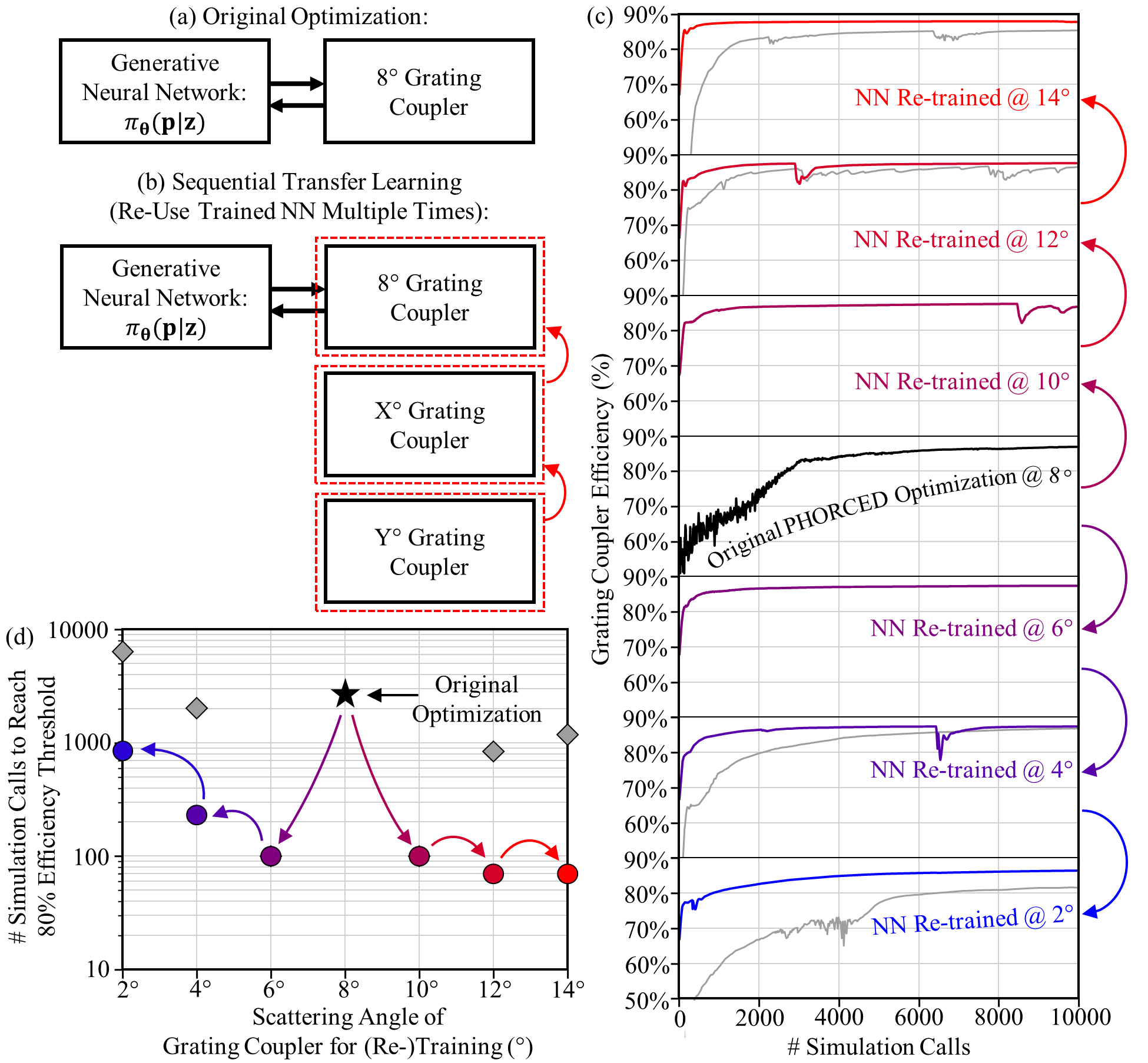
Figure 4: Transfer learning applied sequentially improves convergence for grating coupler scattering angles that are distant relative to the original optimization’s scattering angle. The original PHORCED optimization from Fig. 2(b) is qualitatively depicted in (a) for comparison with the “sequential” transfer learning approach in (b). Here, we sequentially re-train the neural network (originally trained to generate $8^{\circ}$ grating couplers) with progressively different scattering angles, with the intention of slowly changing the physics seen by the neural network. Grating coupler efficiency as a function of the number of simulation calls for each of the re-training sessions are shown in the blue/red curves of (c), where the arrows on the right-hand side show the sequence of each application of transfer learning. The results of the one-shot (non-sequential) transfer learning approach from Fig. 3(c) are shown in gray for comparison. In (d) we plot the number of simulation calls needed for the grating coupler optimizations from (c) to reach an 80% efficiency using the sequential transfer learning approach, similar to the corresponding plot in Fig. 3(d). The blue/red arrows and dots indicate applications of sequential transfer learning, and the gray diamonds correspond to non-sequential transfer learning cases.

Transfer learning applied to grating coupler optimization is qualitatively illustrated in Fig. 3(a)-(b). Fig. 3(a) shows a shorthand version of the PHORCED optimization of Initial Seed 1 that was performed in Fig. 2(b), where a neural network was specifically trained to design an $8^{\circ}$ grating coupler. In the case of transfer learning in Fig. 3(b), we re-use the trained neural network from Fig. 3(a) but now exchange the $8^{\circ}$ angle in the grating coupler efficiency merit function with an alternate scattering angle. In particular, we re-train the neural network on 6 alternative grating coupler angles: {$2^{\circ},4^{\circ},6^{\circ},10^{\circ},12^{\circ},14^{\circ}$}. Note that we maintained the exact same neural network architecture and optimization hyperparameters during these exchanges, including the optimization stopping criterion of 10,000 total simulation calls per training session; the only change in a given optimization was the grating coupler angle. As depicted in Fig. 3(c), we show the optimization progressions of these transfer learning sessions (blue/red curves) in comparison to the original PHORCED optimization of the $8^{\circ}$ grating coupler from Fig. 2(b) (reproduced in the black curve in the middle panel). Also shown are control optimizations for each grating coupler angle using the PHORCED method without transfer learning (in gray). We find that transfer learning to grating couplers with nearby scattering angles (e.g. $6^{\circ}$ and $10^{\circ}$) exhibit extremely accelerated rate of convergence relative to the original optimization and control cases. However, transfer learning is less effective or ineffective for more distant angles (e.g. $2^{\circ}$, $4^{\circ}$, and $14^{\circ}$). This observation is shown more clearly in Fig. 3(d) where we plot the number of simulations required to reach 80% efficiency in optimization versus the scattering angle for re-training . While the original optimization and control optimizations (black star and gray diamonds) required several thousand simulation calls before reaching this threshold, the $6^{\circ}$ and $10^{\circ}$ transfer learning optimizations required only about 100 simulations a piece – a >$10\times$ reduction in simulation calls, making transfer learning comparable with local gradient-based optimization in terms of computation requirements. On the other hand, the distant grating coupler angle transfer learning optimizations ($2^{\circ}$, $4^{\circ}$, and $14^{\circ}$) required similar simulation call requirements to reach the same threshold as the original optimization. Evidently, there is a bias towards less effective transfer learning for small scattering angles. Grating couplers become plagued by parasitic back-reflection for small diffraction angles relative to normal [44, 52], and thus it is possible that the neural network has difficulty adapting to the new physics that were not previously encountered. We conclude that the transfer learning approach is most effective for devices with very similar physics to the device originally optimized by the neural network.

The results of Fig. 3 lead to a natural follow-up query: can we apply transfer learning multiple times progressively in order to maintain the convergence rate advantage for optimizations at more distant grating coupler angles? We explore this question of sequential transfer learning in Fig. 4. In Fig. 4(a)-(b) we qualitatively compare sequential transfer learning to the original PHORCED optimization from Fig. 2(b). As indicated, we replace the original $8^{\circ}$ grating coupler scattering angle in the electromagnetic merit function with an alternative scattering angle in the same manner discussed in Fig. 3(b). Then, after that optimization has completed, we continue to iterate and exchange the grating coupler angle again. By sequentially applying transfer learning, we hope to slowly introduce new physics to the neural network such that we can maintain faster convergence at more physically distant problems from the initial optimization. We conduct two sequential transfer learning sessions where we evolve the grating coupler scattering angle in the following steps: $\{8^{\circ}\rightarrow 10^{\circ}\rightarrow 12^{\circ}\rightarrow 14^{\circ}\}$ and $\{8^{\circ}\rightarrow 6^{\circ}\rightarrow 4^{\circ}\rightarrow 2^{\circ}\}$. The results of these progressions are shown in Fig. 4(c) where we plot the grating coupler efficiency as a function of the number of simulation calls in each (re-)training session. The $6^{\circ}$, $8^{\circ}$, and $10^{\circ}$ cases are the same as those shown previously in Fig. 3(c); the new results may be seen in the $2^{\circ}$, $4^{\circ}$, $12^{\circ}$, and $14^{\circ}$ cases, where blue/red lines indicate the new optimization data and gray lines indicate the non-sequential transfer learning cases from Fig. 3(c) for comparison. We observe that sequential transfer learning improves the optimization convergence rate for the distant grating coupler scattering angles, in accordance with our initial prediction. This observation is made more explicit in Fig. 4(d) where we plot the simulation call requirement to reach an 80% grating coupler efficiency threshold for each of the transfer learning optimizations. Blue/red arrows and points indicate sequential transfer learning progressions, while gray diamonds indicate the one-shot transfer learning cases reproduced from Fig. 3(d). Evidently, sequential transfer learning improves simulation call requirements by approximately an order of magnitude relative to the single-step cases. While we find that there is still a noticeable bias towards longer (but less severely long) training at smaller scattering angles, sequential transfer learning had the added benefit of providing the most efficient devices overall at every scattering angle in the progression. Note that the plotted simulation call requirements do not include the simulation calls from the previous iteration in the sequential transfer learning progression (each application of transfer learning used 10,000 simulation calls, where the final neural network weightset after those 10,000 simulation calls was used as the initial weightset for the next iteration of transfer learning). Furthermore, note that each optimization in these sequential transfer learning cases used the same neural network architecture and hyperparameters as the original PHORCED optimization ($8^{\circ}$ case), except for the $\{12^{\circ}\rightarrow 14^{\circ}\}$ and $\{4^{\circ}\rightarrow 2^{\circ}\}$ cases which required a slightly smaller learning rate in optimization for better performance. The smaller learning rate negligibly affected the 80% efficiency simulation call requirement shown in Fig. 4(d).

5 Conclusion

In this work we introduced PHORCED, a photonic optimization package leveraging the policy gradient method from reinforcement learning. This method interfaces a probablistic neural network with an electromagnetic solver for enhanced inverse design capabilities. PHORCED does not require an evaluation of adjoint method gradient of the electromagnetic merit function with respect to the design parameters, therefore eliminating the need to perform adjoint simulations over the course of an optimization. We anticipate that this fact can be particularly advantageous for multi-frequency electromagnetic merit functions, where multiple adjoint simulations would normally be required in a simple frequency-domain implementation of the adjoint method (e.g., see Ref. [52]).

We applied both PHORCED and the GLOnet method to the proof-of-concept optimization of grating couplers. We found that both algorithms could outperform conventional gradient-based BFGS optimization, resulting in state-of-the-art simulated insertion loss for single-etch c-Si grating couplers and resilience against poor choices of initial condition. In future work we intend to implement fabrication constraints, alternative choices of geometrical parameterization, and other criteria to guarantee feasibility and robustness of experimental devices.

As an additional contribution we introduced the concept of transfer learning to integrated photonic optimization, revealing that a trained neural network using PHORCED could be re-trained on alternative problems with accelerated convergence. In particular, we showed that transfer learning could be applied to the design of grating couplers with varied scattering angle. Transfer learning was extremely effective for grating coupler scattering angles within $\approx\pm 4^{\circ}$ to the original optimization angle, improving the convergence rate by >$10\times$ in some cases. However, this range could be effectively extended to $\approx\pm 6^{\circ}$ or more using a sequential transfer learning approach, where transfer learning was applied multiple times progressively to slowly change the angle seen by the neural network. Because neural network based design methods such as PHORCED are generally data-hungry, we believe that transfer learning could greatly reduce the electromagnetic simulation and compute time that would otherwise be required by these techniques in the design of complex electromagnetic structures. For example, transfer learning could be used in multiple hierarchical stages to evolve an optimization from a two-dimensional structure to a three-dimensional structure, or from a surrogate model (e.g., the grating coupler model in Ref. [10]) to real physics.

Looking forward, we would like to emphasize that PHORCED takes advantage of fundamental concepts in reinforcement learning, but there is a plethora of burgeoning contemporary research in this field, such as advanced policy gradient, off-policy, and model-based approaches. We anticipate that further cross-pollination of the inverse electromagnetic design and reinforcement learning communities could open the floodgates for new research in electromagnetic optimization.

References

- [1] Yichen Shen et al. “Deep Learning with Coherent Nanophotonic Circuits” In Nature Photonics 11.June, 2016, pp. 441–446 DOI: 10.1038/nphoton.2017.93
- [2] Takahiro Inagaki et al. “A coherent Ising machine for 2000-node optimization problems” In Science 354.6312, 2016, pp. 603–606 DOI: 10.1126/science.aah4243
- [3] Nicholas C. Harris et al. “Quantum transport simulations in a programmable nanophotonic processor” In Nature Photonics 11.7, 2017, pp. 447–452 DOI: 10.1038/nphoton.2017.95
- [4] Yoshihisa Yamamoto et al. “Coherent Ising machines—optical neural networks operating at the quantum limit” In npj Quantum Information 3.1, 2017, pp. 1–15 DOI: 10.1038/s41534-017-0048-9
- [5] Erfan Khoram et al. “Nanophotonic media for artificial neural inference” In Photonics Research 7.8, 2019, pp. 823–827 DOI: 10.1364/prj.7.000823
- [6] Tyler W. Hughes, Ian A.. Williamson, Momchil Minkov and Shanhui Fan “Wave physics as an analog recurrent neural network” In Science Advances 5.12, 2019, pp. 1–6 DOI: 10.1126/sciadv.aay6946
- [7] Bhavin J. Shastri et al. “Photonics for artificial intelligence and neuromorphic computing” In Nature Photonics 15.2, 2021, pp. 102–114 DOI: 10.1038/s41566-020-00754-y
- [8] X. Xu et al. “11 TOPS photonic convolutional accelerator for optical neural networks” In Nature 589.7840, 2021, pp. 44–51 DOI: 10.1038/s41586-020-03063-0
- [9] M. Raissi, P. Perdikaris and G.. Karniadakis “Physics-informed neural networks: A deep learning framework for solving forward and inverse problems involving nonlinear partial differential equations” In Journal of Computational Physics 378, 2019, pp. 686–707 DOI: https://doi.org/10.1016/j.jcp.2018.10.045
- [10] Dusan Gostimirovic and Winnie N. Ye “An Open-Source Artificial Neural Network Model for Polarization-Insensitive Silicon-on-Insulator Subwavelength Grating Couplers” In IEEE Journal of Selected Topics in Quantum Electronics 25.3, 2019, pp. 1–5 DOI: 10.1109/JSTQE.2018.2885486
- [11] Yanan Guo, Xiaoqun Cao, Bainian Liu and Mei Gao “Solving Partial Differential Equations Using Deep Learning and Physical Constraints” In Applied Sciences 10.17, 2020, pp. 5917 DOI: 10.3390/app10175917
- [12] Yuyao Chen, Lu Lu, George Em Karniadakis and Luca Dal Negro “Physics-informed neural networks for inverse problems in nano-optics and metamaterials” In Optics Express 28.8, 2020, pp. 11618–11633 DOI: 10.1364/OE.384875
- [13] Raphaël Pestourie et al. “Active learning of deep surrogates for PDEs: application to metasurface design” In npj Computational Materials 6.1, 2020, pp. 1–7 DOI: 10.1038/s41524-020-00431-2
- [14] Abantika Ghosh et al. “Machine Learning-Based Diffractive Image Analysis with Subwavelength Resolution” In ACS Photonics 8.5, 2021, pp. 1448–1456 DOI: 10.1021/acsphotonics.1c00205
- [15] Lu Lu et al. “Physics-informed neural networks with hard constraints for inverse design” In arXiv:2102.04626 [physics], 2021
- [16] Rahul Trivedi et al. “Data-driven acceleration of photonic simulations” In Scientific Reports 9.1, 2019, pp. 1–7 DOI: 10.1038/s41598-019-56212-5
- [17] Yurui Qu et al. “Migrating Knowledge between Physical Scenarios Based on Artificial Neural Networks” In ACS Photonics 6.5, 2019, pp. 1168–1174 DOI: 10.1021/acsphotonics.8b01526
- [18] Daniele Melati et al. “Mapping the global design space of nanophotonic components using machine learning pattern recognition” In Nature Communications 10.1, 2019, pp. 1–9 DOI: 10.1038/s41467-019-12698-1
- [19] Mohammad H. Tahersima et al. “Deep Neural Network Inverse Design of Integrated Photonic Power Splitters” In Scientific Reports 9.1, 2019, pp. 1368 DOI: 10.1038/s41598-018-37952-2
- [20] Anat Demeter-Finzi and Shlomo Ruschin “S-matrix absolute optimization method for a perfect vertical waveguide grating coupler” In Optics Express 27.12, 2019, pp. 16713–16718 DOI: 10.1364/OE.27.016713
- [21] Mohsen Kamandar Dezfouli et al. “Design of fully apodized and perfectly vertical surface grating couplers using machine learning optimization” In Integrated Optics: Devices, Materials, and Technologies XXV 11689 International Society for OpticsPhotonics, 2021, pp. 116890J DOI: 10.1117/12.2576945
- [22] Mahmoud M.. Elsawy et al. “Global optimization of metasurface designs using statistical learning methods” In Scientific Reports 9.1, 2019, pp. 17918 DOI: 10.1038/s41598-019-53878-9
- [23] Alec M. Hammond and Ryan M. Camacho “Designing integrated photonic devices using artificial neural networks” In Optics Express 27.21, 2019, pp. 29620–29638 DOI: 10.1364/OE.27.029620
- [24] J. Jiang and J.. Fan “Global Optimization of Dielectric Metasurfaces Using a Physics-Driven Neural Network” In Nano Letters 19.8, 2019, pp. 5366–5372 DOI: 10.1021/acs.nanolett.9b01857
- [25] Jiaqi Jiang and Jonathan A. Fan “Simulator-based training of generative neural networks for the inverse design of metasurfaces” In Nanophotonics 9.5, 2020, pp. 1059–1069 DOI: doi:10.1515/nanoph-2019-0330
- [26] Jiaqi Jiang and Jonathan A. Fan “Multiobjective and categorical global optimization of photonic structures based on ResNet generative neural networks” In Nanophotonics 10.1, 2020, pp. 361–369 DOI: doi:10.1515/nanoph-2020-0407
- [27] Jiaqi Jiang, Mingkun Chen and Jonathan A. Fan “Deep neural networks for the evaluation and design of photonic devices” In Nature Reviews Materials 6.8, 2021, pp. 679–700 DOI: 10.1038/s41578-020-00260-1
- [28] Ravi S. Hegde “Deep learning: a new tool for photonic nanostructure design” In Nanoscale Advances 2.3, 2020, pp. 1007–1023 DOI: 10.1039/c9na00656g
- [29] Momchil Minkov et al. “Inverse Design of Photonic Crystals through Automatic Differentiation” In ACS Photonics 7.7, 2020, pp. 1729–1741 DOI: 10.1021/acsphotonics.0c00327
- [30] Sunae So et al. “Deep learning enabled inverse design in nanophotonics” In Nanophotonics 2234, 2020, pp. 1–17 DOI: 10.1515/nanoph-2019-0474
- [31] Zihao Ma and Yu Li “Parameter extraction and inverse design of semiconductor lasers based on the deep learning and particle swarm optimization method” In Optics Express 28.15, 2020, pp. 21971 DOI: 10.1364/oe.389474
- [32] Keisuke Kojima et al. “Deep Neural Networks for Inverse Design of Nanophotonic Devices” In Journal of Lightwave Technology 39.4, 2021, pp. 1010–1019 DOI: 10.1109/JLT.2021.3050083
- [33] Wei Ma et al. “Deep learning for the design of photonic structures” In Nature Photonics 15.2, 2021, pp. 77–90 DOI: 10.1038/s41566-020-0685-y
- [34] Daniele Melati et al. “Design of Compact and Efficient Silicon Photonic Micro Antennas with Perfectly Vertical Emission” In IEEE Journal of Selected Topics in Quantum Electronics 27.1, 2021, pp. 1–10 DOI: 10.1109/JSTQE.2020.3013532
- [35] Ravi Hegde “Sample-efficient deep learning for accelerating photonic inverse design” In OSA Continuum 4.3, 2021, pp. 1019–1033 DOI: 10.1364/OSAC.420977
- [36] Jakob S. Jensen and O. Sigmund “Topology optimization for nano-photonics” In Laser and Photonics Reviews 5.2, 2011, pp. 308–321 DOI: 10.1002/lpor.201000014
- [37] J. Lu and J. Vučković “Objective-first design of high-efficiency, small-footprint couplers between arbitrary nanophotonic waveguide modes” In Optics Express 20.7, 2012, pp. 7221–7236 DOI: 10.1364/OE.20.007221
- [38] C.. Lalau-Keraly, S. Bhargava, O.. Miller and E. Yablonovitch “Adjoint shape optimization applied to electromagnetic design” In Optics Express 21.18, 2013, pp. 21693–21701 DOI: 10.1364/OE.21.021693
- [39] Y. Elesin, B.. Lazarov, J.. Jensen and O. Sigmund “Time domain topology optimization of 3D nanophotonic devices” In Photonics and Nanostructures - Fundamentals and Applications 12.1, 2014, pp. 23–33 DOI: 10.1016/j.photonics.2013.07.008
- [40] Alexander Y. Piggott et al. “Inverse design and demonstration of a compact and broadband on-chip wavelength demultiplexer” In Nature Photonics 9.6, 2015, pp. 374–377 DOI: 10.1038/nphoton.2015.69
- [41] L.. Frellsen, Y. Ding, O. Sigmund and L.. Frandsen “Topology optimized mode multiplexing in silicon-on-insulator photonic wire waveguides” In Optics Express 24.15, 2016, pp. 16866–16873 DOI: 10.1364/OE.24.016866
- [42] Logan Su et al. “Fully-automated optimization of grating couplers” In Optics Express 26.4, 2017, pp. 2614–2617 DOI: 10.1364/OE.26.004023
- [43] Andrew Michaels and Eli Yablonovitch “Leveraging continuous material averaging for inverse electromagnetic design” In Optics Express 26.24, 2018, pp. 31717–31737 DOI: 10.1364/OE.26.031717
- [44] Andrew Michaels and Eli Yablonovitch “Inverse design of near unity efficiency perfectly vertical grating couplers” In Optics Express 26.4, 2018, pp. 4766–4779 DOI: 10.1364/OE.26.004766
- [45] Sean Molesky et al. “Inverse design in nanophotonics” In Nature Photonics 12.11, 2018, pp. 659–670 DOI: 10.1038/s41566-018-0246-9
- [46] T.. Hughes, M. Minkov, I… Williamson and S. Fan “Adjoint Method and Inverse Design for Nonlinear Nanophotonic Devices” In ACS Photonics 5.12, 2018, pp. 4781–4787 DOI: 10.1021/acsphotonics.8b01522
- [47] Yingjie Liu et al. “Very sharp adiabatic bends based on an inverse design” In Opt. Lett. 43.11, 2018, pp. 2482–2485 DOI: 10.1364/OL.43.002482
- [48] Nicolas M. Andrade et al. “Inverse design optimization for efficient coupling of an electrically injected optical antenna-LED to a single-mode waveguide” In Optics Express 27.14, 2019, pp. 19802–19814 DOI: 10.1364/OE.27.019802
- [49] Dries Vercruysse et al. “Analytical level set fabrication constraints for inverse design” In Scientific Reports 9.1, 2019, pp. 1–7 DOI: 10.1038/s41598-019-45026-0
- [50] Yannick Augenstein and Carsten Rockstuhl “Inverse Design of Nanophotonic Devices with Structural Integrity” In ACS Photonics 7.8, 2020, pp. 2190–2196 DOI: 10.1021/acsphotonics.0c00699
- [51] Elyas Bayati et al. “Inverse Designed Metalenses with Extended Depth of Focus” In ACS Photonics 7.4, 2020, pp. 873–878 DOI: 10.1021/acsphotonics.9b01703
- [52] Sean Hooten et al. “Adjoint Optimization of Efficient CMOS-Compatible Si-SiN Vertical Grating Couplers for DWDM Applications” In Journal of Lightwave Technology 38.13, 2020, pp. 3422–3430 DOI: 10.1109/JLT.2020.2969097
- [53] Weiliang Jin et al. “Inverse Design of Compact Multimode Cavity Couplers” In Optics Express 26.20, 2018, pp. 26713–26721 DOI: 10.1364/oe.26.026713
- [54] Weiliang Jin, Wei Li, Meir Orenstein and Shanhui Fan “Inverse Design of Lightweight Broadband Reflector for Relativistic Lightsail Propulsion” In ACS Photonics 7.9, 2020, pp. 2350–2355 DOI: 10.1021/acsphotonics.0c00768
- [55] Andrew Michaels, Ming C. Wu and Eli Yablonovitch “Hierarchical Design and Optimization of Silicon Photonics” In IEEE Journal of Selected Topics in Quantum Electronics 26.2, 2020, pp. 1–12 DOI: 10.1109/JSTQE.2019.2935299
- [56] Peng Sun, Thomas Van Vaerenbergh, Marco Fiorentino and Raymond Beausoleil “Adjoint-method-inspired grating couplers for CWDM O-band applications” In Optics Express 28.3, 2020, pp. 3756–3767 DOI: 10.1364/OE.382986
- [57] Zin Lin et al. “End-to-end nanophotonic inverse design for imaging and polarimetry” In Nanophotonics 10.3, 2021, pp. 1177–1187 DOI: 10.1515/nanoph-2020-0579
- [58] Z. Omair, S.. Hooten and E. Yablonovitch “Broadband mirrors with >99% reflectivity for ultra-efficient thermophotovoltaic power conversion” In Energy Harvesting and Storage: Materials, Devices, and Applications XI 11722 International Society for OpticsPhotonics, 2021, pp. 1172208 DOI: 10.1117/12.2588738
- [59] Dries Vercruysse, Neil V. Sapra, Ki Youl Yang and Jelena Vučković “Inverse-Designed Photonic Crystal Devices for Optical Beam Steering” In arXiv:2102.00681 [physics], 2021
- [60] Zhou Zeng, Prabhu K. Venuthurumilli and Xianfan Xu “Inverse Design of Plasmonic Structures with FDTD” In ACS Photonics 8.5, 2021, pp. 1489–1496 DOI: 10.1021/acsphotonics.1c00260
- [61] Ronald J. Williams “Simple statistical gradient-following algorithms for connectionist reinforcement learning” In Machine Learning 8.3, 1992, pp. 229–256 DOI: 10.1007/BF00992696
- [62] Richard S Sutton, David McAllester, Satinder Singh and Yishay Mansour “Policy Gradient Methods for Reinforcement Learning with Function Approximation” In Advances in Neural Information Processing Systems 12 MIT Press, 2000
- [63] A. Michaels “EMopt”, 2019 URL: https://github.com/anstmichaels/emopt
- [64] Louis Faury, Flavian Vasile, Clément Calauzènes and Olivier Fercoq “Neural Generative Models for Global Optimization with Gradients” In arXiv:1805.08594 [cs], 2018
- [65] Louis Faury, Clement Calauzenes, Olivier Fercoq and Syrine Krichen “Improving Evolutionary Strategies with Generative Neural Networks” In arXiv:1901.11271 [cs], 2019
- [66] Nikolaus Hansen “The CMA Evolution Strategy: A Tutorial” In arXiv:1604.00772 [cs, stat], 2016
- [67] Tim Salimans et al. “Evolution Strategies as a Scalable Alternative to Reinforcement Learning” In arXiv:1703.03864 [cs, stat], 2017
- [68] H. Ghraieb et al. “Single-step deep reinforcement learning for open-loop control of laminar and turbulent flows” In Physical Review Fluids 6.5, 2021, pp. 053902 DOI: 10.1103/PhysRevFluids.6.053902
- [69] A. Michaels “GCSlab”, 2019 URL: https://github.com/anstmichaels/gcslab
- [70] Sagi Mathai et al. “Detachable 1x8 single mode optical interface for DWDM microring silicon photonic transceivers” In Optical Interconnects XX 11286 SPIE, 2020, pp. 62–71 International Society for OpticsPhotonics DOI: 10.1117/12.2544400
- [71] Tatsuhiko Watanabe et al. “Perpendicular Grating Coupler Based on a Blazed Antiback-Reflection Structure” In Journal of Lightwave Technology 35.21, 2017, pp. 4663–4669 DOI: 10.1109/JLT.2017.2755673
- [72] Richard S Sutton and Andrew G Barto “Reinforcement learning: An introduction” MIT press, 2018