Cavity optimization for Unruh effect at small accelerations

Abstract

One of the primary reasons behind the difficulty in observing the Unruh effect is that for achievable acceleration scales the finite temperature effects are significant only for the low frequency modes of the field. Since the density of field modes falls for small frequencies in free space, the field modes which are relevant for the thermal effects would be less in number to make an observably significant effect. In this work, we investigate the response of a Unruh-DeWitt detector coupled to a massless scalar field which is confined in a long cylindrical cavity. The density of field modes inside such a cavity shows a resonance structure i.e. it rises abruptly for some specific cavity configurations. We show that an accelerating detector inside the cavity exhibits a non-trivial excitation and de-excitation rates for small accelerations around such resonance points. If the cavity parameters are adjusted to lie in a neighborhood of such resonance points, the (small) acceleration-induced emission rate can be made much larger than the already observable inertial emission rate. We comment on the possibilities of employing this detector-field-cavity system in the experimental realization of Unruh effect, and argue that the necessity of extremely high acceleration can be traded off in favor of precision in cavity manufacturing for realizing non-inertial field theoretic effects in laboratory settings.

Introduction– It is well known that the particle content of a quantum field is observer dependent Fulling-1973 , a fact manifested in numerous theoretical arenas, e.g., the Hawking radiation, cosmic fluctuations, and Unruh effect Hawking-1974 ; Davies-1975 ; Davies-1976 ; Unruh-1976 . In order to estimate the particle content and realize this theoretical idea, the Unruh-DeWitt detector (UDD) Unruh-1976 ; DeWitt-1980 is considered to be an operational device. The UDD is a two-level quantum system with the ground state $|E_{0}\rangle$ and the excited state $|E\rangle$, that is moving along a classical worldline ${\tilde{x}}(\tau)$, where $\tau$ is the proper time in the detector’s frame of reference. The detector is coupled to a quantum field through the interaction Lagrangian ${\cal L}_{\rm int}[\phi({\tilde{x}})]=\alpha m(\tau)\phi[{\tilde{x}}(\tau)]$, where $\alpha$ is a small coupling constant, and $m(\tau)$ is the detector’s monopole moment Unruh-1976 ; DeWitt-1980 which also incorporates a switching function. In the first-order perturbation theory, the transition probability rate of the detector, assuming the scalar field ${\hat{\phi}}$ in its vacuum state $|0\rangle$, is given as ${\dot{P}}(\Delta E)=|\langle E|{\hat{m}}(0)|E_{0}\rangle|^{2}\times{\dot{\cal F}}(\Delta E)$, where ${\dot{\cal F}}(\Delta E)=\int_{-\infty}^{\infty}{\rm d}u~{}e^{-i\Delta Eu}{\cal W}(u,0)$ is called as the response rate of the detector, $\Delta E\equiv E-E_{0}$, and ${\cal W}(x,x^{\prime})\equiv\langle 0|{\hat{\phi}}(x){\hat{\phi}}(x^{\prime})|0\rangle$ is the Wightman function of the field. The UDD probes the vacuum structure of the quantum field through ${\cal W}(x,x^{\prime})$, and registers the excitation of the detector when it absorbs a field quanta. This detector-field system has been popularly employed in investigating the effects of quantum fields in non-inertial frames, since it encompasses the essential aspects of an atom interacting with the electromagnetic field Martinez-2014 . The response rate of a UDD moving in an inertial trajectory can be found to be vanishing, since the vacuum structure of the quantum field in inertial frames is invariant due to Poincaré symmetry Matsas-2008 . However, since non-inertial trajectories are not generated by Poincaré transformations, a UDD moving non-inertially detects particles, a prime example being – for uniform acceleration $a$ the detector shows a non-vanishing thermal response, known as the Unruh effect Unruh-1976 ; DeWitt-1980 ; Matsas-2008 , i.e., ${\dot{\cal F}}=(\Delta E/2\pi)/({\rm e}^{2\pi\Delta E/a}-1)$.

Despite being a fundamental prediction, experimental realization of Unruh effect has not been made possible due to the demand of extremely high accelerations, for appreciable thermal effects one needs $a\geq 10^{21}~{}{\rm m/s}^{2}$ Matsas-2008 . For accelerations small compared to the energy gap $\Delta E$ of the detector, the response rate is exponentially suppressed, i.e., ${\dot{\cal F}}\approx(\Delta E/2\pi){\rm e}^{-2\pi\Delta E/a}$. This suppression basically originates from the fact that the temperature experienced by the accelerating detector is vanishingly small for achievable acceleration scales, since $T\sim\hbar a/{\rm k}_{B}c$. Hence, for such small temperatures, the significant thermal contribution comes only from the low frequency modes, for which the density of field modes (the Bose-Einstein distribution) falls rapidly as $\rho(\omega)\sim\omega^{2}$ in free space, suppressing the response in turn, making experimental verification of Unruh effect a non-trivial exercise of the current era.

In response, efforts have been made to enhance the detector response for maximum achievable accelerations (in foreseeable future) using techniques such as optical cavities Scully-2003 , ultra-intense lasers Chen-1999 ; Habs-2008 , and Penning traps Rogers-1988 . Techniques involving capturing the finite temperature effects of an accelerating system, such as, monitoring thermal quivering Raval-1996 , decay of accelerated protons Vanzella-2001 , and radiation emission in Bose-Einstein condensate Garay-2000 ; Retzker-2008 are also proposed. Other than these, there are attempts using geometric phases Mann-2011 , and properly selected Fock states Fuentes-2010 to enhance the effects of non-inertial motion. Despite these non-trivial attempts, the efforts are still far from the experimental realization of the Unruh effect (however, see Kaminer-2021 for a recent claim).

In this letter, we focus on the low acceleration properties of the UDD inside an optimized cavity. To observe Unruh effect for small accelerations, it is important to characterize scenarios where the density of field modes is increased appreciably, and the correlators of the quantum field are modified non-trivially, so that the detector responds in a distinct manner.

The response rate of a UDD moving along a given trajectory ${\tilde{x}}(\tau)$ can be written in a more general manner as

$${\dot{\cal F}}(\Delta E)\propto\int_{0}^{\infty}{\rm d}\omega_{k}\rho(\omega_{k}){\cal I}(\Delta E,\omega_{k}){\cal J}(\omega_{k},\eta^{i}),$$ (1)

where $\rho(\omega_{k})$ is the density of field modes. The quantity ${\cal I}$ depends on the trajectory of the detector through field correlations, and determines the field modes which stimulate the detector. For example, in the case of inertial detector ${\cal I}(\Delta E,\omega_{k})$ is proportional to $\delta(\Delta E+\omega_{k})$, i.e. only modes with energy $\omega_{k}=-\Delta E$ can contribute to the response rate of the detector, leading to a null response. The function ${\cal J}$ depends on the frequency of the field modes $\omega_{k}$, and the coordinates $\eta^{i}$ that are held fixed on the trajectory of the detector. Therefore, the response rate of the detector can be enhanced by the following ways: (i) Increasing the density of field modes $\rho(\omega_{k})$ at small $\omega_{k}$, say, by changing the boundary conditions, leading to non-trivial changes in the correlators, an aspect missed in the single mode analysis that is usually employed Deb-1997 ; Prants-1999 ; Scully-2003 ; Scully-2006 ; Mann-2011 ; Lopp-2018 . Even for the near resonant frequency modes, the response rate for a single mode Lopp-2018 is suppressed compared to the full-mode analysis (see Supplementary material). The analysis in this paper justifiably makes use of the complete set of modes, and not a few modes that are near the resonant cavity frequency, which gives an additional enhancement channel even at small accelerations; (ii) Choosing the trajectory of the detector appropriately. Even for fixed boundary conditions, different non-inertial trajectories associate different quantum fluctuations to a given inertial field vacuum Letaw-1981 , leading to a change in ${\cal I}(\Delta E,\omega_{k})$ which the detector is sensitive to; (iii) Choosing mechanisms, e.g. the stimulated emission, which are extremely sensitive to both the boundary conditions and the change in field correlations.

Making use of these, we demonstrate that for a uniformly accelerated UDD in a long cylindrical cavity, the acceleration-induced emission rate can be significantly enhanced, even dominating the inertial spontaneous emission, for low accelerations. Uniformly accelerating detector in cavity: Role of resonance points– We consider a UDD inside a cylindrical cavity of radius $R$. The length of the cylindrical cavity is assumed to be much larger than any scale associated with the detector. The scalar field $\phi(x)$ is assumed to satisfy Dirichlet boundary condition i.e., $\phi[\rho=R,\theta,z]=0$ in the cylindrical polar coordinates. The Wightman function corresponding to the scalar field inside the cavity can be expressed as

$${\cal W}(x,x^{\prime}) = \frac{1}{(2\pi R)^{2}}\sum_{m=-\infty}^{\infty}\sum_{n=1}^{\infty}\frac{J_{m}(\xi_{mn}\rho/R)J_{m}(\xi_{mn}\rho^{\prime}/R)}{J^{2}_{|m|+1}(\xi_{mn})}$$ (2)

$$\times \int_{-\infty}^{\infty}\frac{{\rm d}k_{z}}{\omega_{k}}{\rm e}^{-i\omega_{k}(t-t^{\prime}-i\epsilon)}{\rm e}^{im(\theta-\theta^{\prime})}{\rm e}^{ik_{z}(z-z^{\prime})},$$

where $\xi_{mn}$ denotes $n^{{\rm th}}$ zero of the Bessel function $J_{m}(z)$, and $\omega_{k}^{2}=k_{z}^{2}+(\xi_{mn}/R)^{2}$ (see Supplementary material).

For a UDD on a uniformly accelerating trajectory, i.e., ${\tilde{x}}(\tau)=[t,\rho,\theta,z]=(a^{-1}{\rm sinh}a\tau,\rho_{0},\theta_{0},a^{-1}{\rm cosh}a\tau)$, where $\rho_{0}$ and $\theta_{0}$ are constants, and $a$ denotes proper acceleration of the detector,the response rate can be found to be

$${\dot{\cal F}}(\Delta E)=\frac{1}{2\pi}\int_{0}^{\infty}{\rm d}\omega_{k}\underbrace{{\scriptstyle\frac{8}{a^{2}{\rm e}^{\pi\Delta E/a}}\frac{K_{2i\Delta E/a}(2\omega_{k}/a)}{(2\omega_{k}/a)}}}_{{\cal I}(\Delta E,\omega_{k})}$$ (3)

$$\times \sum_{m=-\infty}^{\infty}~{}\underbrace{\sum_{n=1}^{\infty}{\scriptstyle\frac{(\omega_{k}/\pi R^{2})}{J^{2}_{|m|+1}(\xi_{mn})}\frac{\Theta\left(\omega_{k}-\xi_{mn}/R\right)}{\sqrt{\omega_{k}^{2}-(\xi_{mn}/R)^{2}}}}}_{\rho(\omega_{k})}\times\underbrace{{\scriptstyle J_{m}^{2}(\xi_{mn}\rho_{0}/R)}}_{{\cal J}(\rho_{0}/R)},~{}~{}~{}~{}~{}$$

where $K_{\nu}(z)$ is the modified Bessel function of second kind, and $\Theta(x)$ is the Heaviside theta function. One can see that the density of field modes $\rho(\omega_{k})$ has some special features: Firstly, as expected it is independent of the detector parameters – $a$ or $\Delta E$. Secondly, we can see that $\rho(\omega_{k})$ rises abruptly whenever $\omega_{k}^{2}\rightarrow(\xi_{mn}/R)^{2}$, called cavity resonance points, implying the existence of field modes inside the cavity that have very large support in terms of density of states. How such modes contribute to the response rate of the detector is controlled by ${\cal I}(\Delta E,\omega_{k})$. In order to study that, we further evaluate the previous expression to

$${\dot{\cal F}}(\Delta E) = \frac{{\rm e}^{-\pi\Delta E/a}}{\pi^{2}R^{2}a}\sum_{m=-\infty}^{\infty}\sum_{n=1}^{\infty}\frac{J_{m}^{2}(\xi_{mn}\rho_{0}/R)}{J^{2}_{|m|+1}(\xi_{mn})}$$ (4)

$$\times K_{i\Delta E/a}^{2}(\xi_{mn}/Ra).$$

In the limit $a\rightarrow 0$ , the function ${\cal I}(\Delta E,\omega_{k})$ is proportional to $\delta(\Delta E+\omega_{k})$, as expected (see Supplementary material). Thus, in the inertial case there aren’t any modes which contribute to the detector response, including those at the resonance points. However, for the case of non-inertial detector, the function ${\cal I}(\Delta E,\omega_{k})$ allows for the modes around $\omega_{k}\sim\xi_{mn}/R$ to contribute, with some weightage, leading to a non-zero response.

In order to quantify the effects of cavity in enhancing the response rate of the accelerating detector inside the cavity, when compared to the response rate of an accelerating detector in free space ${\dot{\cal F}}_{\cal M}$, we define a quantity ${\cal E}\equiv{\dot{\cal F}}/{\dot{\cal F}}_{\cal M}$, called enhancement in response rate of the detector. In the small acceleration limit, i.e., $a\ll\Delta E$, we make use of the asymptotic expansion of $K_{i\alpha}(\alpha z)$ for large values of $\alpha$ Olver:1974 , with $\alpha\in\mathbb{R}$ and $|{\rm arg}~{}z|<\pi$, to approximate (see Supplementary material)

$${\cal E}\left(\Delta E\right)\approx\frac{4\pi}{(R\Delta E)^{2}}\sum_{m=-\infty}^{\infty}\sum_{n=1}^{\infty}\frac{J_{m}^{2}(\xi_{mn}\rho_{0}/R)}{J^{2}_{|m|+1}(\xi_{mn})}$$

$$\times \begin{cases}\frac{(\beta_{mn}^{<}\Delta E/a)^{1/3}}{\left[1-\left(\frac{\xi_{mn}}{R\Delta E}\right)^{2}\right]^{1/2}}~{}{\rm Ai}^{2}\left[-(\beta_{mn}^{<}\Delta E/a)^{2/3}\right];&\frac{\xi_{mn}}{R\Delta E}<1\\ \\ \frac{1}{3^{4/3}\Gamma^{2}(2/3)}(\Delta E/2a)^{1/3};&\frac{\xi_{mn}}{R\Delta E}=1\\ \\ \frac{(\beta_{mn}^{>}\Delta E/a)^{1/3}}{\left[\left(\frac{\xi_{mn}}{R\Delta E}\right)^{2}-1\right]^{1/2}}~{}{\rm Ai}^{2}\left[(\beta_{mn}^{>}\Delta E/a)^{2/3}\right];&\frac{\xi_{mn}}{R\Delta E}>1\end{cases},$$

where ${\rm Ai}(z)$ is known as the Airy function Olver:1974 , and

$$\beta_{mn}^{<} \equiv \frac{3}{2}{\scriptstyle\left[{\rm sech}^{-1}\left(\frac{\xi_{mn}}{R\Delta E}\right)-\sqrt{1-\left(\frac{\xi_{mn}}{R\Delta E}\right)^{2}}\right]},$$ (6)

$$\beta_{mn}^{>} \equiv \frac{3}{2}{\scriptstyle\left[\sqrt{\left(\frac{\xi_{mn}}{R\Delta E}\right)^{2}-1}-{\rm sec}^{-1}\left(\frac{\xi_{mn}}{R\Delta E}\right)\right]}.$$ (7)

It is evident from Eq.(Cavity optimization for Unruh effect at small accelerations) that in the small acceleration limit the enhancement ${\cal E}$ receives a large amplification, proportional to $(\Delta E/a)^{1/3}$, at the resonance points, i.e., $R\Delta E=\xi_{mn}$. Thus at small accelerations, if one chooses the radius of the cylindrical cavity such that it coincides with one of the resonance points, e.g., $R\Delta E=\xi_{01}=2.405$, the enhancement in response rate ${\cal E}$ shows very large amplifications (see Fig.1).

Though the enhancement in detector response diverges at the resonance points as $\left(\Delta E/a\right)^{1/3}$ in the limit $a/\Delta E\to 0$, the actual response rate of the detector inside the cavity is still small due to the exponential suppression of free space response rate for small accelerations, i.e., $\lim_{a/\Delta E\to 0}{\dot{\cal F}}=\lim_{a/\Delta E\to 0}{\dot{\cal F}}_{\cal M}\times{\cal E}\approx(\Delta E/2\pi){\rm e}^{-2\pi\Delta E/a}\times\lim_{a/\Delta E\to 0}{\cal E}.$ It has been argued in Scully-2003 that the exponential suppression in the response rate inside a cavity can be regulated considerably by introducing non-adiabatic switching of the detector. Now, if the size of the cylindrical cavity is optimized at one of the resonance points in addition to the usage of appropriate switching function, or state selection, as proposed in Scully-2003 , the response rate of the detector can potentially be enhanced exponentially. This line of study, however, will be pursued elsewhere.

In this paper we couple the enhancement in response rate ${\cal E}$ at the resonance points, due to the change in density of field modes $\rho(\omega_{k})$, to another scheme which is extremely sensitive to the change in field correlators, namely the stimulated emission. Since stimulated emission is sensitive to the number of particles present, and a uniformly accelerating detector perceives the Minkowski vacuum as a state with particles, one could expect that a uniformly accelerating detector can undergo stimulated emission. Higher the number of particles in the Minkowski vacuum the detector perceives, higher is its emission rate. The emission profile for a rotating detector was utilized in Lochan-2020 to propose measurable detection of non-inertial quantum field theoretic effects. In Kalinski-2005 the emission from a rotating muonic hydrogen atom in the so called Trojan states is shown to be extremely enhanced. Thus, modifying the density of field modes $\rho(\omega_{k})$ would further strengthen such effects which we analyze next. Acceleration-assisted enhanced emission in cavity: Role of ${\cal I}(-\Delta E,\omega_{k})$– The response rate corresponding to the emission from the UDD can simply be obtained as ${\dot{\cal F}}^{\rm em}\left(\Delta E\right)={\dot{\cal F}}\left(-\Delta E\right)$. One can show that the principle of detailed balance is satisfied for the detector-field system inside the cavity, i.e., ${\dot{\cal F}}^{\rm em}/{\dot{\cal F}}={\rm e}^{2\pi\Delta E/a},$ leading to a thermal distribution of population in equilibrium for a collection of such detectors $n_{g}/n_{e}={\rm e}^{-2\pi\Delta E/a}$, where $n_{g}$ and $n_{e}$ denote the number of detectors in the ground and the excited states respectively.

Since only the function ${\cal I}$ in Eq.(3) is sensitive to $\Delta E\rightarrow-\Delta E$, the emission rate in the cylindrical cavity can be written as

$${\dot{\cal F}}^{\rm em}\left(\Delta E\right)=\frac{1}{\pi R^{2}}\int_{0}^{\infty}{\rm d}\omega_{k}~{}{\cal I}(-\Delta E,\omega_{k})$$ (8)

$$\times \sum_{m=-\infty}^{\infty}\sum_{n=1}^{\infty}\frac{J_{m}^{2}(\xi_{mn}\rho_{0}/R)}{J^{2}_{|m|+1}(\xi_{mn})}\frac{\Theta\left(\omega_{k}-\xi_{mn}/R\right)}{\sqrt{\omega_{k}^{2}-(\xi_{mn}/R)^{2}}}.$$

Note that in the $a\rightarrow 0$ limit ${\cal I}(-\Delta E,\omega_{k})\rightarrow\delta(-\Delta E+\omega_{k})$, so for an inertial detector only the modes with energy $\omega_{k}=\Delta E$ are responsible for the emission of the detector. Since the density of field modes diverges for modes with energy $\omega_{k}=\xi_{mn}/R$, the emission rate becomes divergent if $R\Delta E=\xi_{mn}$, so an inertially moving excited detector emits instantaneously inside such a cavity. On the other hand, for uniformly accelerating detector ${\cal I}(-\Delta E,\omega_{k})\propto a^{-1}{\rm e}^{\pi\Delta E/a}K_{-2i\Delta E/a}(2\omega_{k}/a)$, there is a distribution of modes which determines the emission rate. Some resulting salient features are as follows:

• Since $\delta(-\Delta E+\omega_{k})$ in the expression for inertial emission rate in Eq.(8) is replaced by a smooth function ${\cal I}(-\Delta E,\omega_{k})$, the emission rate of the accelerating detector inside a cavity which is optimized at its resonant configuration $R\Delta E=\xi_{mn}$ is large, but finite. Thus, if the cavity is tuned to be at one of its resonance points, while the inertial detector de-excites in no time, the de-excitation of the accelerating detector takes finite amount of time, the delay marking the non-inertial effect.

• Secondly, due to the change in ${\cal I}(-\Delta E,\omega_{k})$, caused by the accelerated motion, the emission rate of the detector in a cavity, optimized slightly away from the resonance points, is larger than that of an inertial detector (see Fig.1). This is due to the fact that the Delta function (inertial detector) shows a sharper fall off away from the resonance points as compared to the smoother function ${\cal I}(-\Delta E,\omega_{k})$ of the accelerated detector.

Therefore, in comparison to the inertial detector, acceleration of the detector causes a delay in its emission at the resonance points of the cavity, but exhibits substantial enhancement in emission rate slightly away from the resonance points. Further, in the low acceleration limit the enhancement ${\cal E}$ can be related to the emission response rate of the detector ${\dot{\cal F}}^{\rm em}$ as $\lim_{a/\Delta E\to 0}{\dot{\cal F}}^{\rm em}\approx(\Delta E/2\pi)\times\lim_{a/\Delta E\to 0}{\cal E}.$

Figure 1: The emission rates for – the accelerating detector ${\scriptstyle{\dot{\cal F}}^{\rm em}}$ (which is also proportional to the enhancement factor ${\cal E}$ at small accelerations) and the inertial detector ${\scriptstyle{\dot{\tilde{\cal F}}}^{\rm em}}$ w.r.t. $R\Delta E$, with $\rho_{0}=0$, and $a/\Delta E=10^{-3}$. Inset: The discrete plot for the difference in emission rates of the accelerating and the inertial detectors $\Delta{\dot{\cal F}}^{\rm em}$ around the first resonance point $\xi_{01}$. The range of $R\Delta E$ and its step size are chosen such that the contribution exactly at the resonance point $\xi_{01}$ is avoided.

As the enhancement in response rate ${\cal E}$ of the detector exhibits a sharp amplification at the resonance points for small accelerations, one could estimate the amount of non-inertial contribution in the emission rate of the detector at the resonance points of the cavity. In order to further quantify, we subtract the emission rate of an inertial detector ${\scriptstyle{\dot{\cal\widetilde{F}}}^{\rm em}}$ from the non-inertial one, i.e., ${\scriptstyle\Delta{\dot{\cal F}}^{\rm em}\equiv{\dot{\cal F}}^{\rm em}-{\dot{\cal\widetilde{F}}}^{\rm em}}$, obtaining the purely non-inertial contribution in the emission rate slightly away from any resonance point as

$$\Delta{\dot{\cal F}}^{\rm em}\approx\frac{2\Delta E}{(R\Delta E)^{2}}\sum_{m=-\infty}^{\infty}\sum_{n=1}^{\infty}\frac{J_{m}^{2}(\xi_{mn}\rho_{0}/R)}{J^{2}_{|m|+1}(\xi_{mn})}$$

$$\times \begin{cases}\frac{1}{\left[1-\left(\frac{\xi_{mn}}{R\Delta E}\right)^{2}\right]^{1/2}}\{{\scriptstyle(\beta_{mn}^{<}\Delta E/a)^{1/3}{\rm Ai}^{2}\left[-(\beta_{mn}^{<}\Delta E/a)^{2/3}\right]}\\ -\frac{1}{2\pi}\};\hskip 116.65646pt\frac{\xi_{mn}}{R\Delta E}<1\\ \\ \frac{(\beta_{mn}^{>}\Delta E/a)^{1/3}}{\left[\left(\frac{\xi_{mn}}{R\Delta E}\right)^{2}-1\right]^{1/2}}{\scriptstyle{\rm Ai}^{2}\left[(\beta_{mn}^{>}\Delta E/a)^{2/3}\right]};~{}~{}\frac{\xi_{mn}}{R\Delta E}>1\end{cases}.$$

Since $\Delta{\dot{\cal F}}^{\rm em}>0$ amounts to a dominating non-inertial emission, we see (Fig.1) that the emission rate of the accelerating detector can be much higher than that of the inertial detector, if the cavity is designed to be slightly away from one of its resonance points i.e. $Q_{R}\equiv 1-(\xi_{mn}/R\Delta E)^{2}$ is a small (non-zero) number. Since the inertial response diverges at the resonance points, very close to the resonance points $\Delta{\dot{\cal F}}^{\rm em}$ is a large negative number (see Fig.1 (inset)). However, once one starts moving away from the resonance, both inertial and non-inertial emission rates start decaying, with the later decaying much slowly in comparison to the inertial delta function. As a consequence, closer to the resonance point there is a region where the non-inertial response dominates significantly (see Fig.2). Hence, the highly enhanced emission rate of the UDD in a slightly off-resonant cavity will clearly be a distinguishable direct realization of the Unruh effect. Thus, the requirement of high acceleration for observing the Unruh effect can be compensated for a precise cavity design i.e., one with small $Q_{R}$.

Figure 2: The non-inertial contribution to the emission rate $\Delta{\dot{\cal F}}^{\rm em}$ around the first resonance point, i.e., $R\Delta E=\xi_{01}+\epsilon$, w.r.t. $\epsilon$ for various values of $a/\Delta E$ (plots in the top row represent $a/\Delta E=10^{-2},~{}10^{-3}$, while for bottom row $a/\Delta E=10^{-4},~{}10^{-5}$). The black (dotted), red, blue, green, and orange curves correspond to $\beta=0,~{}10^{-4},~{}10^{-3},~{}10^{-2},~{}10^{-1}$ respectively.

Precision in cavity design– Since the non-zero acceleration of the detector allows a width of $R\Delta E$ about any resonance point (see Fig.1 (inset)) where the non-inertial component dominates, we explore the non-inertial component of the emission rate when we go off-resonant by an infinitesimal amount $\epsilon$, i.e., $R\Delta E=\xi_{mn}+\epsilon$. As can be seen in Fig.2, even for smaller value of acceleration ($a/\Delta E\sim 10^{-3}$), with increased precision [$\epsilon\sim(1.5-3)\times 10^{-2}$] in cavity design, the emission rate of the detector is substantially enhanced.

Moreover, in a realistic experimental setup the cylindrical cavity would not be ideal, and the associated $\rho(\omega_{k})$ may not really be diverging at the resonance points, as discussed above. Nevertheless, using a reasonably regularized cavity expressed by $\rho(\omega_{k})\propto 1/[\beta/R+\sqrt{\omega_{k}^{2}-(\xi_{mn}/R)^{2}}]$, with the regularization parameter $\beta\ll 1,$ it can be demonstrated that the dominance of non-inertial contribution near the resonance points is qualitatively independent of the occurrence of divergence in $\rho(\omega_{k})$ (see Fig.2). Further, such near-resonance features remain present for a realistic cavity with leakage of modes as well, which typically provides a Lorentzian broadening for the inertial detectors. In the cylindrical cavity this leakage only modifies the function ${\cal I}(\Delta E,\omega_{k})$, leaving the structure of density of modes $\rho(\omega_{k})$, that harbors the resonance, intact. For achievable quality factors ($\sim 10^{4-6}$) Bertet-2016 ; Zmuidzinas-2010 , the modification in the emission for the case of Rindler motion is only marginal, i.e., $<1\%$ (see the Supplementary material), suggesting the robustness of the scheme. Conclusions– To summarize, for small accelerations $a/\Delta E\to 0$, the enhancement ${\cal E}(\Delta E)$ in the response rate of the accelerating detector inside a long cylindrical cavity diverges as $(\Delta E/a)^{1/3}$ at the resonance points of the cavity, i.e., $\xi_{mn}/R\Delta E=1$. Such resonant configurations of cavity can be utilized very fruitfully for observing the Unruh effect at small accelerations if one couples it with stimulated emission. Since the emission rate of the inertial detector has a sharp fall off away from the resonant frequencies, unlike the accelerating case, to study the non-inertial emission rate of the accelerating detector it is advisable to design a cylindrical cavity to be in a close neighborhood of a resonance point, i.e., $R\Delta E=\xi_{mn}+\epsilon$. In such a cavity, even with small enough acceleration, the non-inertial emission rate can be made much larger than the inertial emission rate and observable. Similar suppression (dominance) of resonant (non-resonant) effects due to the accelerated motion is also observed in recent works Lochan-2020 ; Kempf-2021 .

The calculations presented in this paper can easily be generalized for other fields, e.g. for a UDD with $\Delta E\sim\text{MHz}$ (e.g. Hydrogen atom making a $2p\rightarrow 2s$ transition Lochan-2020 ) inside an optical cavity. The required dimensions of the cavity for such atoms could be $(\ell\sim aT^{2}\gg a/\Delta E^{2}\sim\text{cm}$ and $R\sim\xi_{mn}/\Delta E\sim\text{cm})$. For such dimensions even a marginal acceleration $a\sim 10^{9}ms^{-2}$, that can easily be obtained for instance by setting up a thermal gradient Gallina of $\Delta T=(ma/k_{B})\Delta x\sim 1K$ across the cavity of $\Delta x\sim cm$, leads to a significant emission enhancement. Further, multiple non-interacting accelerated particles, e.g. a beam of UDDs, can be sent inside the cavity, and an integrated enhanced effect can be observed to further strengthen the signal Blencowe-2021 .

Appendix A Appendix: Supplementary material

We consider a Unruh-DeWitt detector, with the ground state $|E_{0}\rangle$ and the excited state $|E\rangle$, coupled to a massless scalar field $\phi(x)$ which is confined inside a cylindrical cavity of radius $R$. The confined scalar field satisfies Dirichlet boundary condition. The interaction between the detector and the scalar field is described by the interaction Lagrangian ${\cal L}_{\rm int}[\phi({\tilde{x}}(\tau)]=\alpha m(\tau)\phi({\tilde{x}}(\tau)$. If the initial state of the detector-field system is $|0\rangle\otimes|E_{0}\rangle$, and the final state is $|{\bf k}\rangle\otimes|E\rangle$, where $|0\rangle$ and $|{\bf k}\rangle$ are respectively the vacuum state and the one-particle state of the scalar field, then the transition probability associated with this process in the first-order perturbation theory can be written as

$${\cal A}_{\bf k}=i\langle E|\otimes\langle{\bf k}|\int_{-\infty}^{\infty}{\rm d}\tau{\hat{m}}(\tau){\hat{\phi}}[{\tilde{x}}(\tau)]|0\rangle\otimes|E_{0}\rangle.$$ (10)

Integrating over all possible one-particle states of the field, one can obtain the transition probability as

$$P_{E_{0}\to E} = |\langle E|{\hat{m}}(0)|E_{0}\rangle|^{2}$$

$$\times \int_{-\infty}^{\infty}\int_{-\infty}^{\infty}{\rm d}\tau{\rm d}\tau^{\prime}{\rm e}^{-i\Delta E(\tau-\tau^{\prime})}{\cal W}[x(\tau),x(\tau^{\prime})],$$

where ${\cal W}(x,x^{\prime})=\langle 0|{\hat{\phi}}(x){\hat{\phi}}(x.)|0\rangle$ is the Wightman function corresponding to the field.

If the detector is allowed to move along the integral curve of a Killing vector field, then the transition probability can be reduced to transition probability rate as

$${\dot{P}}(\Delta E)\equiv\lim_{v\to\infty}\frac{P_{E_{0}\to E}}{v}=|\langle E|{\hat{m}}(0)|E_{0}\rangle|^{2}\times{\dot{\cal F}}(\Delta E),$$ (12)

where ${\dot{\cal F}}$ is called as response rate of the detector, and is

$${\dot{\cal F}}(\Delta E)=\int_{-\infty}^{\infty}{\rm d}u{\rm e}^{-i\Delta Eu}{\cal W}(u,0),$$ (13)

with $u=\tau-\tau^{\prime}$ and $v=(\tau+\tau^{\prime})/2$. Note that the response rate ${\dot{\cal F}}$ of the detector is just the Fourier transform of the pullback of the Wightman function on the trajectory of the detector.

The scalar field ${\hat{\phi}}$ confined inside the cavity satisfying Dirichlet boundary condition is

$${\hat{\phi}}(x) = \frac{1}{2\pi R}\sum_{m=-\infty}^{\infty}\sum_{n=1}^{\infty}\frac{J_{m}(\xi_{mn}r/R)}{J_{|m|+1}(\xi_{mn})}\int_{-\infty}^{\infty}\frac{{\rm d}k_{z}}{\sqrt{\omega_{k}}}$$

$$\times \left({\hat{a}}_{\bf k}{\rm e}^{-i\omega_{k}t}{\rm e}^{im\theta}{\rm e}^{ik_{z}z}+{\hat{a}}^{\dagger}_{\bf k}{\rm e}^{i\omega_{k}t}{\rm e}^{-im\theta}{\rm e}^{-ik_{z}z}\right),$$

where $[{\hat{a}}_{\bf k},{\hat{a}}^{\dagger}_{\bf k^{\prime}}]=\delta_{mm^{\prime}}\delta_{nn^{\prime}}\delta(k_{z}-k^{\prime}_{z})$, $[{\hat{a}}_{\bf k},{\hat{a}}_{\bf k^{\prime}}]=0$, and $[{\hat{a}}^{\dagger}_{\bf k},{\hat{a}}^{\dagger}_{\bf k^{\prime}}]=0$. Making use of the expression for the field ${\hat{\phi}}$ inside the cavity, we find the Wightman function as

$${\cal W}(x,x^{\prime}) = \frac{1}{(2\pi R)^{2}}\sum_{m=-\infty}^{\infty}\sum_{n=1}^{\infty}\frac{J_{m}(\xi_{mn}\rho/R)J_{m}(\xi_{mn}\rho^{\prime}/R)}{J^{2}_{|m|+1}(\xi_{mn})}$$ (15)

$$\times \int_{-\infty}^{\infty}\frac{{\rm d}k_{z}}{\omega_{k}}{\rm e}^{-i\omega_{k}(t-t^{\prime}-i\epsilon)}{\rm e}^{im(\theta-\theta^{\prime})}{\rm e}^{ik_{z}(z-z^{\prime})},$$

where $\omega_{k}^{2}=(\xi_{mn}/R)^{2}+k_{z}^{2}$.

Substituting the trajectory of an accelerating detector $[t=a^{-1}{\rm sinh}(a\tau),\rho=\rho_{0},\theta=\theta_{0},z=a^{-1}{\rm cosh}(a\tau)]$ in the expression for Wightman function, and using it in the expression for response rate ${\dot{\cal F}}$ of the detector, we find

$${\dot{\cal F}}(\Delta E) = \frac{2}{(2\pi R)^{2}}\sum_{m=-\infty}^{\infty}\sum_{n=1}^{\infty}\frac{J_{m}^{2}(\xi_{mn}\rho_{0}/R)}{J^{2}_{|m|+1}(\xi_{mn})}$$

$$\times \int_{0}^{\infty}{\rm d}\omega_{k}\frac{\Theta(\omega_{k}-\xi_{mn}/R)}{\sqrt{\omega_{k}^{2}-(\xi_{mn}/R)^{2}}}$$

$$\times \int_{-\infty}^{\infty}{\rm d}ue^{-i\Delta Eu}{\rm exp}\left\{-2i(\omega_{k}/a){\rm sinh}(au/2)\right\}.$$

In the limit $a\to 0$ in Eq.(A), we arrive at the response rate of the inertial detector inside the cavity as

$${\dot{\cal F}}(\Delta E)=\frac{1}{\pi R^{2}}\sum_{m=-\infty}^{\infty}\sum_{n=1}^{\infty}\frac{J_{m}^{2}(\xi_{mn}\rho_{0}/R)}{J^{2}_{|m|+1}(\xi_{mn})}$$ (17)

$$\times \int_{0}^{\infty}{\rm d}\omega_{k}\frac{\Theta(\omega_{k}-\xi_{mn}/R)}{\sqrt{\omega_{k}^{2}-(\xi_{mn}/R)^{2}}}~{}\delta(\Delta E+\omega_{k}),$$

which is vanishing since the argument of the delta function is positive throughout the range of $\omega_{k}$.

Evaluating the integrals in the expression for response rate of the accelerating detector in Eq.(A), we obtain

$${\dot{\cal F}}(\Delta E) = \frac{1}{\pi^{2}R}\frac{{\rm e}^{-\pi\Delta E/a}}{Ra}\sum_{m=-\infty}^{\infty}\sum_{n=1}^{\infty}\frac{J_{m}^{2}(\xi_{mn}\rho_{0}/R)}{J^{2}_{|m|+1}(\xi_{mn})}$$ (18)

$$\times K_{i\Delta E/a}^{2}(\xi_{mn}/Ra).$$

Making use of the asymptotic expansion of $K_{i\alpha}(\alpha x)$ for large positive values of $\alpha$ Olver:1974 , which is

$${\scriptstyle K_{i\alpha}(\alpha x)=\frac{{\rm e}^{-\pi\alpha/2}}{\sqrt{\alpha}}\pi\sqrt{2}}\begin{cases}{\scriptstyle\frac{(\beta^{<}\alpha)^{1/6}}{\left(1-x^{2}\right)^{1/4}}~{}{\rm Ai}\left[-(\beta^{<}\alpha)^{2/3}\right];}&{\scriptstyle x<1}\\ \\ {\scriptstyle\frac{\alpha^{1/6}}{3^{2/3}\Gamma(2/3)}};&{\scriptstyle x=1}\\ \\ {\scriptstyle\frac{(\beta^{>}\alpha)^{1/6}}{\left(x^{2}-1\right)^{1/4}}~{}{\rm Ai}\left[(\beta^{>}\alpha)^{2/3}\right];}&{\scriptstyle x>1}\end{cases},$$ (19)

where ${\rm Ai}(z)$ is the Airy function, with

$$\beta^{<} \equiv \frac{3}{2}\left({\rm sech}^{-1}x-\sqrt{1-x^{2}}\right),$$ (20)

$$\beta^{>} \equiv \frac{3}{2}\left(\sqrt{x^{2}-1}-{\rm sec}^{-1}x\right),$$ (21)

in Eq.(18), we obtain

$${\dot{\cal F}}(\Delta E)\approx\frac{2}{R}\frac{{\rm e}^{-2\pi\Delta E/a}}{R\Delta E}\sum_{m=-\infty}^{\infty}\sum_{n=1}^{\infty}\frac{J_{m}^{2}(\xi_{mn}\rho_{0}/R)}{J^{2}_{|m|+1}(\xi_{mn})}$$

$$\times \begin{cases}\frac{(\beta_{mn}^{<}\Delta E/a)^{1/3}}{\left[1-\left(\frac{\xi_{mn}}{R\Delta E}\right)^{2}\right]^{1/2}}~{}{\rm Ai}^{2}\left[-(\beta_{mn}^{<}\Delta E/a)^{2/3}\right];&\frac{\xi_{mn}}{R\Delta E}<1\\ \\ \frac{1}{3^{4/3}\Gamma^{2}(2/3)}(\Delta E/2a)^{1/3};&\frac{\xi_{mn}}{R\Delta E}=1\\ \\ \frac{(\beta_{mn}^{>}\Delta E/a)^{1/3}}{\left[\left(\frac{\xi_{mn}}{R\Delta E}\right)^{2}-1\right]^{1/2}}~{}{\rm Ai}^{2}\left[(\beta_{mn}^{>}\Delta E/a)^{2/3}\right];&\frac{\xi_{mn}}{R\Delta E}>1\end{cases},$$

where

$$\beta_{mn}^{<} \equiv \frac{3}{2}{\scriptstyle\left[{\rm sech}^{-1}\left(\frac{\xi_{mn}}{R\Delta E}\right)-\sqrt{1-\left(\frac{\xi_{mn}}{R\Delta E}\right)^{2}}\right]},$$

$$\beta_{mn}^{>} \equiv \frac{3}{2}{\scriptstyle\left[\sqrt{\left(\frac{\xi_{mn}}{R\Delta E}\right)^{2}-1}-{\rm sec}^{-1}\left(\frac{\xi_{mn}}{R\Delta E}\right)\right]}.$$

Appendix B Contribution due to a single-mode

When it comes to investigating the interaction of atoms with quantum fields confined inside cavities, it is quite common to employ the single-mode approximation where the field inside the cavity is assumed to be the field modes that are in resonance with the resonant configuration of the cavity Deb-1997 ; Prants-1999 ; Scully-2003 ; Mann-2011 ; Lopp-2018 . Recently it was shown that the single-mode approximation becomes inaccurate when it comes to trajectories of detectors/atoms that are relativistic and non-inertial Lopp-2018 . The enhancement discussed in this paper at low accelerations around the resonant configurations of the cavity is due to the divergence in the density of field modes $\rho(\omega_{k})$, which cannot be captured by the single-mode analysis. To see this, we write the scalar field inside a cylindrical cavity of finite length $L$ with boundary conditions

$$\phi(\rho=R,\phi,z) = 0,$$ (23)

$$\phi(\rho,\phi,z=\pm L/2) = 0,$$ (24)

as

$${\hat{\phi}}(t,{\bf x})=\frac{1}{\sqrt{\pi R^{2}L}}\sum_{l=-\infty}^{\infty}\sum_{m=-\infty}^{\infty}\sum_{n=1}^{\infty}\frac{J_{m}(\xi_{mn}\rho/R)}{J_{|m|+1}(\xi_{mn})}$$ (25)

$$\times \Biggl{\{}{\hat{a}}_{k}\Biggl{[}\frac{1}{\sqrt{2\omega^{(s)}_{k}}}{\rm cos}\left(\frac{(2l+1)\pi}{L}z\right){\rm e}^{-i\omega^{(s)}_{k}t}$$

$$+ \frac{i}{\sqrt{2\omega^{(a)}_{k}}}{\rm sin}\left(\frac{2l\pi}{L}z\right){\rm e}^{-i\omega^{(a)}_{k}t}\Biggr{]}{\rm e}^{im\theta}$$

$$+ {\hat{a}}^{\dagger}_{k}\Biggl{[}\frac{1}{\sqrt{2\omega^{(s)}_{k}}}{\rm cos}\left(\frac{(2l+1)\pi}{L}z\right){\rm e}^{i\omega^{(s)}_{k}t}$$

$$- \frac{i}{\sqrt{2\omega^{(a)}_{k}}}{\rm sin}\left(\frac{2l\pi}{L}z\right){\rm e}^{i\omega^{(a)}_{k}t}\Biggr{]}{\rm e}^{-im\theta}\Biggr{\}},$$

with $k\equiv(l,m,n)$, $\omega^{(s)}_{k}=\sqrt{\left(\frac{\xi_{mn}}{R}\right)^{2}+\left(\frac{(2l+1)\pi}{L}\right)^{2}}$, $\omega^{(a)}_{k}=\sqrt{\left(\frac{\xi_{mn}}{R}\right)^{2}+\left(\frac{2l\pi}{L}\right)^{2}}$, and

$$[{\hat{a}}_{k},{\hat{a}}_{k^{\prime}}^{\dagger}]=\delta_{ll^{\prime}}\delta_{mm^{\prime}}\delta_{nn^{\prime}},$$ (26)

$$[{\hat{a}}_{k},{\hat{a}}_{k^{\prime}}]=0,~{}~{}[{\hat{a}}_{k}^{\dagger},{\hat{a}}_{k^{\prime}}^{\dagger}]=0.$$ (27)

The Wightman function corresponding to the field confined inside the cavity can be found to be

$${\cal W}(x,x^{\prime})=\frac{1}{\pi R^{2}L}\sum_{l=-\infty}^{\infty}\sum_{m=-\infty}^{\infty}\sum_{n=1}^{\infty}$$ (28)

$$\times \frac{J_{m}(\xi_{mn}\rho/R)}{J_{|m|+1}(\xi_{mn})}\frac{J_{m}(\xi_{mn}\rho^{\prime}/R)}{J_{|m|+1}(\xi_{mn})}{\rm e}^{im(\theta-\theta^{\prime})}$$

$$\times \Biggl{\{}\frac{1}{2\omega^{(s)}_{k}}{\rm cos}\left(\frac{(2l+1)\pi}{L}z\right){\rm cos}\left(\frac{(2l+1)\pi}{L}z^{\prime}\right)$$

$$\times {\rm e}^{-i\omega^{(s)}_{k}(t-t^{\prime})}$$

$$- \frac{i}{2\sqrt{\omega^{(s)}_{k}\omega^{(a)}_{k}}}{\rm cos}\left(\frac{(2l+1)\pi}{L}z\right){\rm sin}\left(\frac{2l\pi}{L}z^{\prime}\right)$$

$$\times {\rm e}^{-i\omega^{(s)}_{k}t}{\rm e}^{i\omega^{(a)}_{k}t^{\prime}}$$

$$+ \frac{i}{2\sqrt{\omega^{(s)}_{k}\omega^{(a)}_{k}}}{\rm sin}\left(\frac{2l\pi}{L}z\right){\rm cos}\left(\frac{(2l+1)\pi}{L}z^{\prime}\right)$$

$$\times {\rm e}^{i\omega^{(s)}_{k}t^{\prime}}{\rm e}^{-i\omega^{(a)}_{k}t}$$

$$+ \frac{1}{2\omega^{(a)}_{k}}{\rm sin}\left(\frac{2l\pi}{L}z\right){\rm sin}\left(\frac{2l\pi}{L}z^{\prime}\right)$$

$$\times {\rm e}^{-i\omega^{(a)}_{k}(t-t^{\prime})}\Biggr{\}}.$$

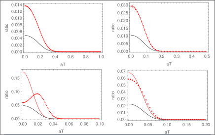
Figure 3: The ratio $r$ of emission rates due to a (symmetric) single-mode ($l^{\prime}=0,~{}m^{\prime}=0,~{}n^{\prime}=1$) and complete set of modes around the first resonance point, i.e., $R\Delta E=\xi_{01}$, is plotted with respect to. $aT$ for various values of $a/\Delta E$ (clockwise from left top, $a/\Delta E=10^{-2},~{}10^{-3},~{}10^{-4},~{}10^{-5}$). The dotted red, black, and joined red curves correspond to $R\Delta E-\xi_{01}=-10^{-3},0,10^{-3}$ respectively. Note that we have assumed $L/R=10^{3}$ for all the plots.

If one assumes the length $L$ of the cavity is much larger that the length scales involved in the system, i.e., $a^{-1}$, $\Delta E^{-1}$, and $R$, then the finite-time ($T$) response rate of the uniformly accelerating detector can be evaluated as

$$\dot{\cal F}\left(\Delta E\right)\approx\frac{{\rm e}^{-\pi\Delta E/a}}{\pi(aR)RL}\sum_{l=-\infty}^{\infty}\sum_{m=-\infty}^{\infty}\sum_{n=1}^{\infty}\frac{J^{2}_{m}(\xi_{mn}\rho_{0}/R)}{J^{2}_{|m|+1}(\xi_{mn})}$$ (29)

$$\times \Biggl{\{}\Biggl{(}\frac{1}{\omega^{(s)}_{k}}{\rm cos}\left[\frac{\Delta E}{a}\ln\left(\frac{L\omega^{(s)}_{k}-(2l+1)\pi}{L\omega^{(s)}_{k}+(2l+1)\pi}\right)\right]$$

$$- \frac{1}{\omega^{(a)}_{k}}{\rm cos}\left[\frac{\Delta E}{a}\ln\left(\frac{L\omega^{(a)}_{k}-2l\pi}{L\omega^{(a)}_{k}+2l\pi}\right)\right]\Biggr{)}$$

$$\times K_{2i\Delta E/a}\left(\frac{2\xi_{mn}}{Ra}{\rm cosh}aT\right)$$

$$+ \frac{1}{\omega^{(s)}_{k}}K_{2i\Delta E/a}\left[\frac{2}{a}\left(\omega^{(s)}_{k}{\rm cosh}aT-\frac{(2l+1)\pi}{L}{\rm sinh}aT\right)\right]$$

$$+ \frac{1}{\omega^{(a)}_{k}}K_{2i\Delta E/a}\left[\frac{2}{a}\left(\omega^{(a)}_{k}{\rm cosh}aT-\frac{2l\pi}{L}{\rm sinh}aT\right)\right]\Biggr{\}}.$$

Choosing one particular (symmetric) mode $\omega^{(s)}_{k^{\prime}}$ we calculate the response rate ${\dot{\cal F}}^{(s)}_{\rm sm}$ of the detector due to this single-mode to be

$${\dot{\cal F}}^{(s)}_{\rm sm}\left(\Delta E\right)\approx\frac{{\rm e}^{-\pi\Delta E/a}}{\pi(aR)RL}\frac{J^{2}_{m^{\prime}}(\xi_{m^{\prime}n^{\prime}}\rho_{0}/R)}{J^{2}_{|m^{\prime}|+1}(\xi_{m^{\prime}n^{\prime}})}$$

$$\times \Biggl{\{}\frac{1}{\omega^{(s)}_{k^{\prime}}}{\rm cos}\left[\frac{\Delta E}{a}\ln\left(\frac{L\omega^{(s)}_{k^{\prime}}-(2l^{\prime}+1)\pi}{L\omega^{(s)}_{k^{\prime}}+(2l^{\prime}+1)\pi}\right)\right]$$

$$\times K_{2i\Delta E/a}\left(\frac{2\xi_{m^{\prime}n^{\prime}}}{Ra}{\rm cosh}aT\right)$$

$$+ \frac{1}{\omega^{(s)}_{k^{\prime}}}K_{2i\Delta E/a}\left[\frac{2}{a}\left(\omega^{(s)}_{k^{\prime}}{\rm cosh}aT-\frac{(2l^{\prime}+1)\pi}{L}{\rm sinh}aT\right)\right]\Biggr{\}}.$$

Using this we calculate the ratio $r\equiv{\dot{\cal F}}^{(s)}_{\rm sm}/{\dot{\cal F}}$ to compare the response rate due to the single-mode viz-a-viz the same due to the complete set of modes, and plot it with respect to $aT$ as shown in Fig.(3). It is evident from Fig.(3) that the contribution due to a single-mode is insignificant in the late-time limit ($T\to\infty$) against the contribution due to the complete set of field modes Lopp-2018 . Also, the single-mode approximation evidently misses the near-resonance ($R\Delta E\approx\xi_{mn}$) enhancement in the response rate brought in by the complete set of field modes, particularly through the density of field modes $\rho(\omega_{k})$.

Appendix C Cavity with Loss

For realistic cavities with non-zero leakage, assuming the field encompasses the information about dissipation, one could write

$${\hat{\phi}}(t,{\bf x})=\frac{1}{2\pi R}\sum_{m=-\infty}^{\infty}\sum_{n=1}^{\infty}{\rm e}^{-\alpha_{mn}|t|}\frac{J_{m}(\xi_{mn}r/R)}{J_{|m|+1}(\xi_{mn})}$$

$$\times \int_{-\infty}^{\infty}\frac{{\rm d}k_{z}}{\sqrt{\omega_{k}}}\left({\hat{a}}_{{\bf k}}{\rm e}^{-i\omega_{k}t}{\rm e}^{im\theta}{\rm e}^{ik_{z}z}+{\hat{a}}^{\dagger}_{{\bf k}}{\rm e}^{i\omega_{k}t}{\rm e}^{-im\theta}{\rm e}^{-ik_{z}z}\right),$$

where $\alpha_{mn}=\xi_{mn}/RQ$ are the inertial leakage factors of the modes inside the cavity, and they depend on the quality factor $Q$ of the cavity. Making use of this in the two point function, we obtain the expression for the emission probability of the detector as

$${\cal P}(\Delta E) = \int_{-\infty}^{\infty}{\rm d}v\int_{-\infty}^{\infty}{\rm d}ue^{i\Delta Eu}\langle 0|{\hat{\phi}}(\tau){\hat{\phi}}(\tau^{\prime})|0\rangle$$ (32)

$$\equiv \int_{0}^{\infty}{\rm d}v~{}{\dot{\cal F}}^{\text{em}}_{Q}(\Delta E),$$

where $u=\tau-\tau^{\prime}$ and $v=(\tau+\tau^{\prime})/2$. The emission response rate of an inertial detector, i.e., the trajectory of the detector be $(\gamma\tau,\rho_{0},\theta_{0},\gamma v\tau)$, can be found to be $v$ dependent as

$${\dot{\cal F}}^{\text{em}}_{Q}\left(\Delta E\right)=\int_{0}^{\infty}{\rm d}\omega_{k}$$

$$\times \sum_{m=-\infty}^{\infty}~{}\sum_{n=1}^{\infty}{\scriptstyle\frac{(\omega_{k}/\pi R^{2})}{J^{2}_{|m|+1}(\xi_{mn})}\frac{\Theta\left(\omega_{k}-\xi_{mn}/R\right)}{\sqrt{\omega_{k}^{2}-(\xi_{mn}/R)^{2}}}}$$

$$\times {\scriptstyle{\rm e}^{-2\gamma\alpha_{mn}v}\Biggl{\{}\left[1-\frac{(\omega_{k}-\Delta E)^{2}}{[(\gamma\alpha_{mn})^{2}+(\omega_{k}-\Delta E)^{2}]}\right]\frac{{\rm sin}[2(\omega_{k}-\Delta E)v]}{(\omega_{k}-\Delta E)}}$$

$$+ {\scriptstyle\frac{\gamma\alpha_{mn}}{[(\gamma\alpha_{mn})^{2}+(\omega_{k}-\Delta E)^{2}]}~{}{\rm cos}[2(\omega_{k}-\Delta E)v]\Biggr{\}}\times\frac{J_{m}^{2}(\xi_{mn}\rho_{0}/R)}{\omega_{k}}}.$$

In the zero loss limit ($\{\alpha_{mn}\}\to 0$) we obtain the standard inertial expression for the emission rate as

$${\dot{\cal F}}^{\text{em}}_{Q\to\infty}(\Delta E)=\frac{1}{\pi R^{2}}\sum_{m=-\infty}^{\infty}\sum_{n=1}^{\infty}\frac{J_{m}^{2}(\xi_{mn}\rho_{0}/R)}{J^{2}_{|m|+1}(\xi_{mn})}$$ (34)

$$\times \int_{0}^{\infty}{\rm d}\omega_{k}\frac{\Theta\left(\omega_{k}-\xi_{mn}/R\right)}{\sqrt{\omega_{k}^{2}-(\xi_{mn}/R)^{2}}}\delta(\omega_{k}-\Delta E).$$

In the limit $v\to 0$, the rate has a Lorentzian support for various modes

$$\lim_{v\to 0}{\dot{\cal F}}^{\text{em}}_{Q}(\Delta E)=\int_{0}^{\infty}{\rm d}\omega_{k}$$ (35)

$$\times \sum_{m=-\infty}^{\infty}~{}\underbrace{\sum_{n=1}^{\infty}{\scriptstyle\frac{(\omega_{k}/\pi R^{2})}{J^{2}_{|m|+1}(\xi_{mn})}\frac{\Theta\left(\omega_{k}-\xi_{mn}/R\right)}{\sqrt{\omega_{k}^{2}-(\xi_{mn}/R)^{2}}}}}_{\rho(\omega_{k})}$$

$$\underbrace{{\scriptstyle\frac{\gamma\alpha_{mn}}{\omega_{k}[(\gamma\alpha_{mn})^{2}+(\omega_{k}-\Delta E)^{2}]}}}_{{\cal I}(-\Delta E,\omega_{k})}\times\underbrace{{\scriptstyle J_{m}^{2}(\xi_{mn}\rho_{0}/R)}}_{{\cal J}(\rho_{0}/R)}.$$

Similarly, the emission rate of the detector in a non-inertial Rindler trajectory, i.e., $[a^{-1}{\rm sinh}(a\tau),\rho_{0},\theta_{0},a^{-1}{\rm cosh}(a\tau)]$ in the limit $av\to 0$ can be obtained as

$$\lim_{av\to 0}{\dot{\cal F}}^{\text{em}}_{Q}(\Delta E)=\int_{0}^{\infty}{\rm d}\omega_{k}$$

$$\times \sum_{m=-\infty}^{\infty}\underbrace{\sum_{n=1}^{\infty}{\scriptstyle\frac{(\omega_{k}/\pi R^{2})}{J^{2}_{|m|+1}(\xi_{mn})}\frac{\Theta\left(\omega_{k}-\xi_{mn}/R\right)}{\sqrt{\omega_{k}^{2}-(\xi_{mn}/R)^{2}}}}}_{\rho(\omega_{k})}\times\underbrace{{\scriptstyle J_{m}^{2}(\xi_{mn}\rho_{0}/R)}}_{{\cal J}(\rho_{0}/R)}$$

$$\times \underbrace{{\scriptstyle\frac{1}{\omega_{k}}\text{Re}\Biggl{(}\int_{0}^{\infty}du~{}e^{i\Delta Eu}{\rm exp}\left[-i\frac{2(\omega_{k}+\alpha_{mn})}{a}{\rm sinh}(au/2)\right]\Biggr{)}}}_{{\cal I}(-\Delta E,\omega_{k})},$$

$$=\frac{1}{\pi^{2}R}\frac{(2\Delta E/a)}{(R\Delta E)}\sum_{m=-\infty}^{\infty}\sum_{n=1}^{\infty}\frac{J_{m}^{2}(\xi_{mn}\rho_{0}/R)}{J^{2}_{|m|+1}(\xi_{mn})}$$

$$\times \text{Re}\biggl{\{}\int_{0}^{\infty}dx~{}e^{-(2\Delta E/a)\left[(R\alpha_{mn}/R\Delta E)\sinh x-ix\right]}$$

$$\times K_{0}\left[i(2\Delta E/a)\frac{\xi_{mn}}{R\Delta E}{\rm sinh}x\right]\biggr{\}},$$ (37)

which for the no loss case $(\{\alpha_{mn}\}=0)$ reproduces Eq.4. In the limit $av\to 0$, the departure in emission rate from the same for an ideal cavity (no loss) for various values of the quality factor can be computed by evaluating the integral in Eq.(37).

$Q$	${\dot{\cal F}}^{\text{em}}_{Q}/\Delta E$	$(1-{\dot{\cal F}}^{\text{em}}_{Q}/{\dot{\cal F}}^{\text{em}}_{Q\to\infty})\times 100\%$
$10^{3}$	$\sim 1.226$	$~{}~{}~{}~{}~{}~{}~{}\sim 3\%$
$10^{4}$	$\sim 1.259$	$~{}~{}~{}~{}~{}~{}~{}\sim 0.3\%$
$10^{5}$	$\sim 1.262$	$~{}~{}~{}~{}~{}~{}~{}\sim 0.03\%$
$10^{6}$	$\sim 1.263$	$~{}~{}~{}~{}~{}~{}~{}\sim 0.003\%$

Table 1: The $Q$-modified emission rate and the $\%$ deviation of the same from the lossless ($Q\to\infty$) emission rate for different quality factors.

An estimate for the emission rate in a realistic cavity set up $(\Delta E\sim\text{MHz};a\sim 10^{12}ms^{-2};\rho_{0}=0;R\Delta E=\xi_{01}+0.1$) is presented in Table 1.

References

• (1) S. A. Fulling, Phys. Rev. D 7, 2850 (1973)
• (2) S. W. Hawking, Nature (London) 248, 30 (1974).
• (3) P. C. W. Davies, Journal of Physics A, 8, 609 (1975).
• (4) P. C. W. Davies, Nature (London) 263, 377 (1976).
• (5) W. G. Unruh, Phys. Rev. D 14, 870 (1976).
• (6) B. S. DeWitt, in General Relativity; an Einstein Centenary Survey, edited by S. W. Hawking and W. Israel (Cambridge University Press, Cambridge, England, 1980).
• (7) E. Martín-Martínez, M. Montero, and M. del Rey, Phys. Rev. D 87, 064038 (2013); A. M. Alhambra, A. Kempf, and E. Martín-Martínez, Phys. Rev. A 89, 033835 (2014).
• (8) L. C. B. Crispino, A. Higuchi, and G. E. A. Matsas, Rev. Mod. Phys. 80, 787 (2008).
• (9) M. O. Scully, V. V. Kocharovsky, A. Belyanin, E. Fry, and F. Capasso, Phys. Rev. Lett. 91, 243004 (2003).
• (10) P. Chen and T. Tajima, Phys. Rev. Lett. 83, 256 (1999).
• (11) R. Schutzhold, G. Schaller, and D. Habs, Phys. Rev. Lett. 100, 091301 (2008).
• (12) J. Rogers, Phys. Rev. Lett. 61, 2113 (1988).
• (13) A. Raval, B. L. Hu, and J. Anglin, Phys. Rev. D 53, 7003 (1996).
• (14) D. A. T. Vanzella and G. E. A. Matsas, Phys. Rev. Lett. 87, 151301 (2001).
• (15) L. J. Garay, J. R. Anglin, J. I. Cirac and P. Zoller, Phys. Rev. Lett. 85, 4643 (2000).
• (16) A. Retzker, J. I. Cirac, M. B. Plenio, and B. Reznik, Phys. Rev. Lett. 101, 110402 (2008).
• (17) E. Martín-Martínez, I. Fuentes, and R. B. Mann, Phys. Rev. Lett. 107, 131301 (2011).
• (18) M. Aspachs, G. Adesso, and I. Fuentes, Phys. Rev. Lett. 105, 151301 (2010).
• (19) M. H. Lynch, E. Cohen, Y. Hadad, and I. Kaminer, Phys. Rev. D 104, 025015 (2021).
• (20) B. Deb and S. Sen, Phys. Rev. A 56, 2470 (1997).
• (21) S. V. Prants, L. E. Konkov, and I. L. Kirilyuk, Phys. Rev. E 60, 335 (1999).
• (22) A. Belyanin, V. V. Kocharovsky, F. Capasso, E. Fry, M. S. Zubairy, and M. O. Scully, Phys. Rev. A 74, 023807 (2006).
• (23) R. Lopp, E. Martin-Martinez, and D. N. Page, Class. Quantum Grav., 35, 224001 (2018).
• (24) J. R. Letaw, Phys. Rev. D 23, 1709 (1981).
• (25) F. Olver, Asymptotics and special functions, A K Peters, Massachusetts (1974).
• (26) K. Lochan, H. Ulbricht, A. Vinante, and S. K. Goyal, Phys. Rev. Lett. 125, 241301 (2020).
• (27) M. Kalinski, Laser Physics 15, 10 (2005).
• (28) A. Bienfait, J. J. Pla, Y. Kubo, X. Zhou, M. Stern, C. C. Lo, C. D. Weis, T. Schenkel, D. Vion, D. Esteve, J. J. L. Morton, and P. Bertet, Nature (London) 531, 74 (2016).
• (29) H. G. Leduc, B. Bumble, P. K. Day, B. H. Eom, J. Gao, S. Golwala, B. A. Mazin, S. McHugh, A. Merrill, D. C. Moore, O. Noroozian, A. D. Turner, and J. Zmuidzinas, Appl. Phys. Lett. 97, 102509 (2010).
• (30) B. Soda, V. Sudhir, and A. Kempf, arXiv:2103.15838 [quant-ph] (2021).
• (31) V. Gallina, and M. Omini, Nuov Cim B 8, 65 (1972).
• (32) H. Wang, M. Blencowe, Commun Phys 4, 128 (2021).