Abstract:

Deep neural network (DNN) is a popular model implemented in many systems to handle complex tasks such as image classification, object recognition, natural language processing etc. Consequently DNN structural vulnerabilities become part of the security vulnerabilities in those systems. In this paper we study the root cause of DNN adversarial examples. We examine the DNN response surface to understand its classification boundary. Our study reveals the structural problem of DNN classification boundary that leads to the adversarial examples. Existing attack algorithms can generate from a handful to a few hundred adversarial examples given one clean image. We show there are infinitely many adversarial images given one clean sample, all within a small neighborhood of the clean sample. We then define DNN uncertainty regions and show transferability of adversarial examples is not universal. We also argue that generalization error, the large sample theoretical guarantee established for DNN, cannot adequately capture the phenomenon of adversarial examples. We need new theory to measure DNN robustness.

Key Words:

Adversarial Machine Learning, Deep Neural Network, Response Surface, Uncertainty Regions, DNN Classification Boundary

1 Introduction

DNN is a powerful tool for complex tasks, such as image classification, object recognition etc., especially when there are thousands of object classes. Pictures of connected nodes are often displayed to illustrate the structure of DNN. DNN generates feature maps from an input that are most strongly associated with the learning task. Pooling layers, such as max pooling, can further identify the features. And the popular activation function, the Rectified Non-Linear Unit (ReLU), aims to solve the vanishing gradient problem [20]. One earliest application of DNN was to classify handwritten images [32]. Starting with the success of AlexNet on the ImageNet classification task [29], DNN has regained popularity over other classifiers. Soon afterwards, researchers noticed that targetedly adding minor perturbations to a clean image can cause a DNN to misclassify the perturbed image [57]. This is the beginning of a new chapter on adversarial machine learning research.

There are real world implications when using DNN in critical applications without fully understanding its properties, such as its classification boundary and vulnerabilities. For example, Tesla uses camera and radar as sensors. DNN is used to process the videos received from cameras, as described on the webpage for Tesla AutopilotAI.   Soon Tesla Model 3 and Y vehicles will ditch radar and rely only on cameras.   In a system where the algorithm used to process sensor data has inherent vulnerabilities, they become part of the security vulnerabilities the attackers can explore. Notice Tesla suffered high profile fatal crashes where its Autopilot was suspected to play a role.    

The cause of the adversarial examples is a mystery until now. So far there are only conflicting conjectures. [57, 12] believed adversarial examples lie in “dense pockets” in lower dimensional manifold, caused by DNN’s non-linearity. On the other hand [21] believed it is DNN’s linear nature and the very high dimensional inputs that lead to the adversarial examples. Furthermore [21] used Figure 4 to show “adversarial examples occur in contiguous regions of the 1-D subspace defined by the fast gradient sign method, not in fine pockets.” Although Explainable Artificial Intelligence (XAI) becomes a hot research area, aiming to decipher DNN internal components, there is still a lack of understanding of one most basic concept of DNN – the shape of its classification boundary. For example, [60] showed the classification boundary of DNN as a curve in Figure 3, and the adversarial region was on the other side of the classification boundary in Figure 1.

In this paper we study DNN’s classification boundary through its response surface. Through experiments, we show the problem of adversarial examples is not as simple as linear vs. non-linear. It is a far more complex structural problem. Response surface methodology is a well studied subject in statistics. A response variable $y$ is influenced by several independent variables $x_{1}$, …, $x_{k}$. The relationship is modeled or approximated by a function with an error term, $y=h(x_{1},...,x_{k})+\epsilon$. The response surface describes the relationship between $y$ and $x_{1}$, …, $x_{k}$. Response surface methodology plays an important role in design of experiments, e.g., [30, 39]. We notice that along with the research on response surface methodology, design robustness and design uncertainty received considerable attention since [8, 9, 10].

We know the response surface of many well known models, such as linear regression, generalized linear regression, non-parametric regression, to name a few. For supervised learning techniques, support vector machine (SVM) uses hyper-planes to separate the data points; linear discriminant analysis has a linear decision boundary; quadratic discriminant analysis has non-linear decision boundary. Despite many work on building a robust DNN and to evaluate DNN robustness, we are yet to know the shape of DNN classification boundary. Without the knowledge of DNN classification boundary, building a robust DNN model will remain an elusive task. The most significant contributions of this paper are the following.

1. We show DNN classification boundary is highly fractured, unlike other classifiers. The adversarial examples exist in lower dimensional hyper-rectangles within a small neighborhood surrounding each clean image,

2. We show that transferability of adversarial examples is not universal, contrary to [57, 21, 60]. [57, 21, 60] suggested that adversarial examples generated against one DNN are misclassified by other DNNs, even if they have different model structures or are trained on different subsets of the training data. We show that adversarial examples against one DNN can be correctly classified by other DNN models, simply by using different initial random seeds in the training process. This leads to our definition of DNN uncertainty regions.

3. We argue that generalization error, which measures DNN large sample performance, cannot adequately capture the phenomenon of adversarial examples. New theory is needed to measure DNN robustness.

Besides the three major contributions, additional contributions of this paper are the following.

1. Given one clean image, existing attack algorithms generate up to a few hundred adversarial examples through an optimization approach. Sampling from the lower dimensional hyper-rectangles lead to a stronger attack – we have infinitely many adversarial examples given one clean image.

2. Far fewer pixels are perturbed to form these hyper-rectangles compared to the existing attack algorithms. Therefore we reduce the total amount of perturbations added to a clean image to create adversarial examples.

3. Training a DNN is a non-convex optimization problem. There are many local optima. By using different initial values, we obtain different trained DNN models. Some benchmark attacks, such as Carlini & Wagner $L_{2}$ attack, often attacks the target model only. Our adversarial examples can attack multiple models simultaneously.

The paper is organized as follows. Section 1.1 discusses the related work. Section 2 conducts experiments to show DNN response surface and introduces the concept of DNN uncertainty regions. Section 3 discusses the discrepancy between the theoretically proven DNN generalization error bound and the existence of adversarial examples. Section 4 concludes this paper.

1.1 Related Work

There is an extensive literature on robust statistics, e.g., [23, 47]. Robust regression, robust tests, and robust estimators have been developed to address the problems where the true distribution deviates from the model assumption, and outliers. Adversarial machine learning also aims to build robust learning models, but under a different scenario – adversaries discover the vulnerabilities of a learning model, which cause the learning model to make a costly mistake. There are two broad categories of attacks, poisoning attacks and evasion attacks [63]. Poisoning attacks inject malicious samples into the training data, to cause the resulting learning model to make a mistake with certain test samples. Assuming there is no easy access to the training process, evasion attacks generate test samples that the learning model cannot handle correctly. The adversarial examples generated to attack DNN belong to evasion attacks.

Adversarial (evasion) attacks against DNN are the earliest attacks. Recently there are attacks designed to break graph neural network (e.g., [67, 58]), recurrent neural network (e.g., [43, 13, 18, 51, 52]), and deep reinforcement learning (e.g., [34, 22, 46, 5]). In this paper, we study the response surface and uncertainty regions of DNN, i.e., convolutional neural network (CNN) or fully connected neural network (multilayer perceptron (MLP)). There are many existing attacks against such DNN models. In our experiments we use Foolbox [16], which implemented 42 attack algorithms. Depending on adversaries’ knowledge of a DNN model, there are white-box attacks and black-box attacks. For white-box attacks, adversaries know the true DNN model, including model structure and parameter values. For black-box attacks, adversaries don’t know the true model. Instead, adversaries query the true model, build a local substitute model based on the queries, and attack the local model. A targeted attack generates adversarial examples that are misclassified into a pre-determined class, while an untargeted attack simply generates misclassified samples.

Several survey papers are published, introducing the current state and the timeline of attacks and defenses, e.g., [2, 7, 63]. In general, the attack algorithms follow an optimization approach, i.e., generating adversarial examples while minimizing their distances to the clean samples. Let $W$ be a clean image and $W^{a}$ be an adversarial example. Let $M$ be a trained DNN model that assigns a class label to $W$. We have $M(W^{a})\neq M(W)$. $W$ is a matrix for a gray-scale image, and a tensor for a color image. The size of the matrix/tensor is determined by the image resolution. The individual elements (pixels) in $W$ represent the light level, having integer values ranging from 0 (no light) to 255 (maximum light). The pixels are often rescaled to $[0,1]$. $W$ can be vectorized. Our approach needs close to a hundred adversarial images $W^{a}$ given one clean image $W$. Some attack algorithms generate a single $W^{a}$ or only a handful of $W^{a}$s are not used in our experiments. We also exclude attack algorithms that need large perturbations to generate $W^{a}$, since the resulting adversarial images will be outside of a small $\delta$ neighborhood of the clean image $W$. Here we introduce the attack algorithms that are used in our experiments.

• Pointwise (PW) Attack [50]: An effective decision-based attack minimizing $||W^{a}-W||_{0}$, i.e., the number of pixels in $W$ and $W^{a}$ that have different values.

• Carlini & Wagner $L_{2}$ (CW2) Attack [11]: $W^{a}$ is generated by minimizing $\textrm{Distance}(W,W^{a})+a\times\textrm{loss}(W^{a})$. $L_{1}$, $L_{2}$, and $L_{\infty}$ norms are considered. The $L_{2}$ distance is the most commonly used.

• NewtonFool (NF) Attack [26]: The perturbation follows the gradient that reduces the probability $W^{a}$ belongs to the correct class $c$.

• Fast Gradient Sign Method (FGSM) [21]: Given a loss function, $W^{a}$ is generated as $W^{a}=W-\epsilon\times\textrm{sign}(\nabla\textrm{loss}(W))$. $\epsilon$ is the step size, usually a small number for producing minor perturbation. FGSM follows the sign of the gradient of the loss function. It generates adversarial examples much faster than Carlini & Wagner attack.

• Basic Iterative Method (BIM) [31]: It improves FGSM attack by clipping the pixel values in each iteration to reduce the amount of perturbation added to $W$. $L_{1}$, $L_{2}$ and $L_{\infty}$ distance can be used in the attack.

• Moment Iterative (MI) Attack [14]: It applies momentum to accelerate the gradient descent in a set-up similar to FGSM while escaping local maxima with poor results.

2 DNN Response Surface and Uncertainty Regions

DNN’s response surface is described by $M(W)=c$, where $c$ is the object class assigned to image $W$ by a trained DNN model $M$. In this paper we assume $M$ assigns hard labels. The response surface is more complex, when $W$ is a high resolution color image with $M$ assigning soft labels, and classification accuracy is assessed using top 5 classes. We leave it to the future work.

Uncertainty regions are proposed for SVM facing multi-class classification task. For one-against-all SVM, multiple separating hyper-planes are used to classify the samples. The areas within the margins of the binary hyper-planes are the SVM uncertainty regions [45, 24, 62, 61]. Meaning if a data point is very close to multiple binary decision boundaries, SVM is uncertain which class it belongs to.

We propose a different definition of DNN uncertainty regions. Given a training dataset $D_{n}$ with $n$ samples, let $\mathcal{M}=\{M_{1},M_{2},...\}$ be the set of DNN models with identical model structure, i.e., same number of layers, same activation, etc. $M_{i}\in\mathcal{M}$ is obtained by having a DNN model trained on $D_{n}$ and varying the initial seeds. Since DNN training is a non-convex optimization problem, they converge to different local optima. For $i\neq j$, $M_{i}$ and $M_{j}$ have different parameter values. Define DNN uncertainty region as follows.

Definition 1.

An uncertainty region is defined as $U~{}:=~{}\left\{W:\exists~{}M_{i},~{}M_{j}~{}\in\mathcal{M},~{}s.t.~{}M_{i}(W)~{}\neq~{}M_{j}(W)\right\}$.

In a small $\delta-$neighborhood of a clean image $W$, $\delta>0$, a perturbed image $W^{a}$ is a noisy but recognizable version of the clean image $W$. We use the $L_{2}$ distance between $W$ and $W^{a}$, $d(W,W^{a})=||W-W^{a}||_{2}$. Define $B(\delta,W)$ as $B(\delta,W)~{}:=~{}\left\{W:~{}d(W^{a},W)\leq\delta\right\}.$ Inside $B(\delta,W)$ with $\delta$ sufficiently small, ideally a classifier should assign all the noisy images to the same object class of $W$.

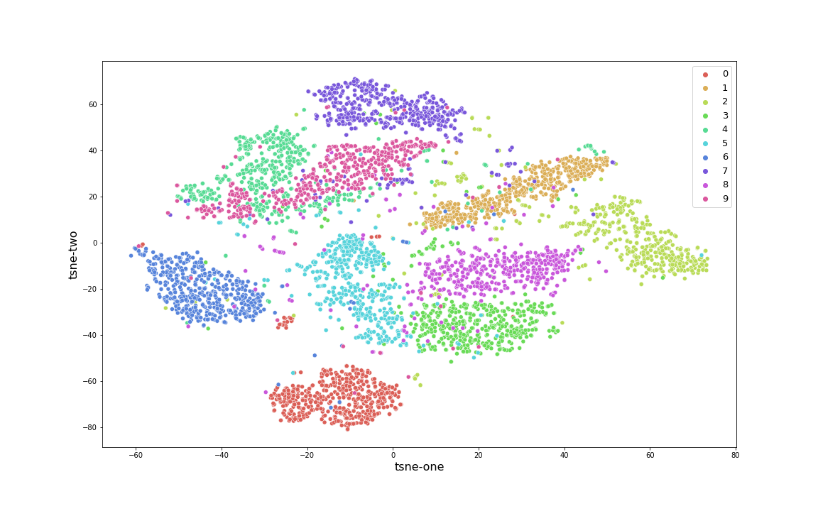
Figure 1: Lower Dimensional Projection of MNIST data

Table 1: CNN Mis-classification Rates on Clean MNIST Test Images

$M_{1}$	$M_{2}$	$M_{3}$	$M_{4}$	$M_{5}$	$M_{6}$	$M_{7}$	$M_{8}$	$M_{9}$	$M_{10}$
0.033	0.035	0.025	0.019	0.017	0.015	0.013	0.012	0.012	0.012

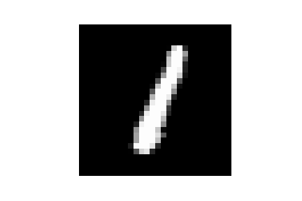
Figure 2: Clean Test Image 1

Table 2: CNN Misclassification Rates in Hyper-Rectangles

	$s_{(i)}$	$M_{1}$	$M_{2}$	$M_{3}$	$M_{4}$	$M_{5}$	$M_{6}$	$M_{7}$	$M_{8}$	$M_{9}$	$M_{10}$
PW 30d $1\to 2$	1	0.843	0.454	0.281	0.344	0.183	0.58	0.687	0.596	0.709	0.848
CW2 280d $1\to 2$	0.0001	0.929	0	0	0	0	0	0	0	0	0
BIM $L_{1}$ 240d $1\to 2$	0.016	0.429	0.445	0.461	0.427	0.406	0.426	0.453	0.441	0.444	0.450
NF 60d $1\to 2$	0.030	0	0	0	0.001	0.004	0.925	1	0.58	0.991	1
FGSM 375d $1\to 2$	0.012	0.915	0	0	0	0	0	0	0	0	0
CW2 210d $1\to 3$	0.008	0.855	0.01	0.843	0.974	1	1	0.998	0.984	0.999	1
BIM $L_{1}$ 230d $1\to 3$	0.016	0.458	0.456	0.484	0.482	0.472	0.466	0.462	0.469	0.497	0.480
BIM $L_{2}$ 200d $1\to 3$	0.019	0.706	0.734	0.669	0.698	0.698	0.672	0.701	0.718	0.685	0.708
MI 320d $1\to 3$	0.036	0.91	0	0	0	0	0	0	0	0	0
CW2 180d $1\to 4$	0.009	0.999	0	0	0	0	0	0	0	0	0
CW2 175d $1\to 5$	0.011	0.047	0	0.135	1	1	1	1	1	1	1
MI 205d $1\to 5$	0.036	0.991	0.041	0	1	0.916	1	0.845	0.035	0.907	1
CW2 150d $1\to 6$	0.013	0	0.099	0	0.993	0.007	0.945	0.807	0.042	1	0.652
BIM $L_{2}$ 220d $1\to 6$	0.003	0.448	0.455	0.472	0.454	0.407	0.432	0.421	0.449	0.431	0.421
CW2 220d $1\to 7$	0.003	0.871	0	0	0	0	0	0	0	0	0
BIM $L_{1}$ 200d $1\to 7$	0.028	0.826	0.81	0.824	0.812	0.832	0.811	0.825	0.813	0.801	0.828
BIM $L_{\infty}$ 380d $1\to 7$	0.002	0.782	0	0	0	0	0	0	0	0	0
MI 300d $1\to 7$	0.028	0.999	0	0	0	0	0	0	0	0	0
PW 35d $1\to 8$	1	0.809	0.818	0.48	0.856	0.896	0.974	0.932	0.754	0.92	0.937
CW2 190d $1\to 8$	0.0004	0.847	0	0	0.014	0.655	0.009	0	0	0	0
BIM $L_{1}$ 240d $1\to 8$	0.002	0.389	0.37	0.365	0.363	0.365	0.37	0.365	0.384	0.36	0.351
MI 280d $1\to 8$	0.006	0.908	0.909	0.908	0.900	0.930	0.919	0.904	0.911	0.918	0.917
CW2 200d $1\to 9$	0.025	0.995	0	0.01	0.97	1	1	0	0.022	0.396	0.99
BIM $L_{1}$ 140d $1\to 9$	0.013	0.651	0.001	0.008	0.252	0.503	0.758	0.071	0.244	0.013	0.182
CW2 200d $1\to 0$	0.005	0	0	0	0	0	1	0.946	0	1	1
BIM $L_{1}$ 120d $1\to 0$	0.036	0.761	0.714	0.751	0.724	0.738	0.748	0.722	0.742	0.743	0.752
BIM $L_{2}$ 120d $1\to 0$	0.030	0.928	0.95	0.935	0.927	0.924	0.931	0.937	0.93	0.92	0.932
BIM $L_{\infty}$ 350d $1\to 0$	0.003	0.527	0.868	0.127	0.227	0.02	0.007	0	0	0	0
MI 230d $1\to 0$	0.032	0.996	1	0	0.235	0	0	0	0	0	1

Table 3: $L_{2}$ Distance

	$L_{2}^{min}$	$L_{2}^{max}$	$\bar{L}_{2}$	$L_{2}^{min}$ Attack	$L_{2}^{max}$ Attack	$\bar{L}_{2}$ Attack
PW $1\to 2$	4.885	14.27	9.578	11.063	26.462	17.388
CW2 $1\to 2$	3.061	3.131	3.093	3.066	3.14	3.096
BIM $L_{1}$ $1\to 2$	2.915	3.455	3.165	3.091	3.514	3.164
NF $1\to 2$	4.881	5.729	5.305	4.986	8.803	6.806
FGSM $1\to 2$	14.259	14.41	14.335	14.413	15.213	14.784
CW2 $1\to 3$	7.948	11.91	8.879	5.663	16.674	8.467
BIM $L_{1}$ $1\to 3$	5.195	6.287	5.641	5.531	6.43	5.63
BIM $L_{2}$ $1\to 3$	4.403	6.081	5.042	5.504	7.732	5.631
MI $1\to 3$	10.406	11.112	10.695	16.457	21.854	20.135
CW2 $1\to 4$	6.385	6.87	6.528	6.591	6.924	6.743
CW2 $1\to 5$	10.743	12.989	11.567	9.932	16.703	12.298
MI $1\to 5$	17.502	19.526	18.514	34.122	48.086	43.28
CW2 $1\to 6$	7.285	8.435	7.86	7.485	12.687	9.719
BIM $L_{2}$ $1\to 6$	6.557	9.689	8.123	7.101	9.891	8.641
CW2 $1\to 7$	4.493	4.716	4.575	4.519	4.721	4.58
BIM $L_{1}$ $1\to 7$	5.039	7.565	6.002	5.321	7.614	5.69
BIM $L_{\infty}$ $1\to 7$	8.197	9.124	8.661	13.118	15.11	14.855
MI $1\to 7$	8.892	9.457	9.075	14.633	18.742	17.377
PW $1\to 8$	5.205	14.84	10.023	12.526	26.526	17.329
CW2 $1\to 8$	3.604	4.281	3.843	3.722	4.572	3.917
BIM $L_{1}$ $1\to 8$	3.316	4.009	3.562	3.637	4.188	3.778
MI $1\to 8$	8.569	9.158	8.863	9.615	14.493	13.126
CW2 $1\to 9$	11.062	11.276	11.069	10.975	12.52	11.586
BIM $L_{1}$ $1\to 9$	8.636	12.579	10.608	10.38	14.186	11.741
CW2 $1\to 0$	10.099	11.218	10.644	11.661	11.932	11.813
BIM $L_{1}$ $1\to 0$	9.231	11.994	10.255	12.733	20.247	14.552
BIM $L_{2}$ $1\to 0$	11.299	16.77	14.035	12.279	19.563	14.216
BIM $L_{\infty}$ $1\to 0$	12.392	15.827	14.11	34.519	79.041	39.734
MI $1\to 0$	21.261	22.607	21.852	43.76	43.297	38.818

Table 4: CNN Attack Misclassification Rates

	$M_{1}$	$M_{2}$	$M_{3}$	$M_{4}$	$M_{5}$	$M_{6}$	$M_{7}$	$M_{8}$	$M_{9}$	$M_{10}$
PW 38d $1\to 2$	1	0.02	0	0.02	0.04	0.27	0.23	0.27	0.30	0.49
CW2 286d $1\to 2$	1	0	0	0	0	0	0	0	0	0
BIM $L_{1}$ 425d $1\to 2$	1	0	0	0	0	0	0	0	0	0
NF 403d $1\to 2$	1	0.82	0.62	0.92	0.96	1	1	0.95	1	1
FGSM 403d $1\to 2$	1	0	0	0	0	0	0	0	0	0
CW2 263d $1\to 3$	1	0	0	0	0	0	0	0	0	0
BIM $L_{1}$ 455d $1\to 3$	1	0	0	0	0.01	0.14	0.01	0	0.01	0.05
BIM $L_{2}$ 454d $1\to 3$	1	0.01	0.02	0.08	0.11	0.23	0.06	0.02	0.09	0.12
MI 427d $1\to 3$	1	0	0	0.44	0.41	0.62	0.30	0.03	0.41	0.49
CW2 310d $1\to 4$	1	0	0	0	0	0	0	0	0	0
CW2 308d $1\to 5$	1	0	0	0	0	0	0	0	0	0
MI 489d $1\to 5$	1	1	1	1	1	1	1	1	1	1
CW2 318d $1\to 6$	1	0	0	0	0	0	0	0	0	0
BIM $L_{2}$ 483d $1\to 6$	1	1	0.19	1	0.12	0.98	0.46	0.05	1	0.28
CW2 258d $1\to 7$	1	0	0	0	0	0	0	0	0	0
BIM $L_{1}$ 460d $1\to 7$	1	0.02	0.03	0.03	0.03	0.02	0	0	0.11	0.32
BIM $L_{\infty}$ 491d $1\to 7$	1	0	0	0	0	0	0	0	0	0
MI 473d $1\to 7$	1	0	0	0	0	0	0	0	0	0.30
PW 40d $1\to 8$	1	0.04	0.01	0.15	0.16	0.55	0.37	0.41	0.33	0.48
CW2 258d $1\to 8$	1	0	0	0	0	0	0	0	0	0
BIM $L_{1}$ 424d $1\to 8$	1	0	0	0	0	0.07	0	0	0	0
MI 438d $1\to 8$	1	0	0	0.55	0	0.05	0	0	0	0
CW2 314d $1\to 9$	1	0	0	0	0	0	0	0	0	0
BIM $L_{1}$ 492d $1\to 9$	1	0.55	0.94	0.98	0.99	0.99	0.90	0.74	0.93	0.96
CW2 286d $1\to 0$	1	0	0	0	0	0	0	0	0	0
BIM $L_{1}$ 496d $1\to 0$	1	0.91	0.62	0.83	0.76	0.89	0.79	0.68	0.92	0.91
BIM $L_{2}$ 495d $1\to 0$	1	0.91	0.30	0.70	0.55	0.85	0.63	0.43	0.76	0.76
BIM $L_{\infty}$ 510d $1\to 0$	1	1	0.98	0.98	0.96	0.98	0.87	0.52	0.59	0.52
MI 462d $1\to 0$	1	1	0.95	1	0.87	0.85	0.82	0.62	0.63	0.67

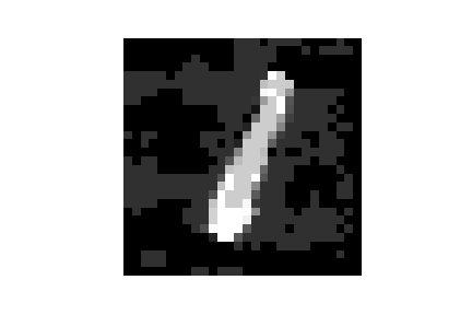
(a) FGSM $1\to 2$

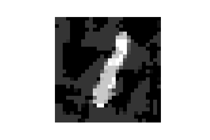
(b) MI $1\to 3$

(c) CW2 $1\to 4$

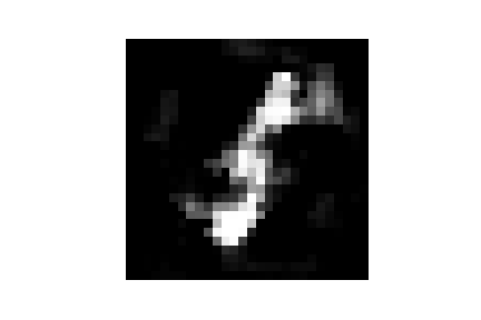
(d) CW2 $1\to 5$

(e) BIM $L_{2}$ $1\to 6$

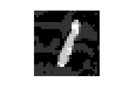
(f) MI $1\to 7$

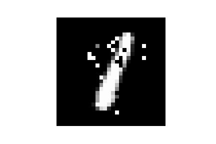
(g) PW $1\to 8$

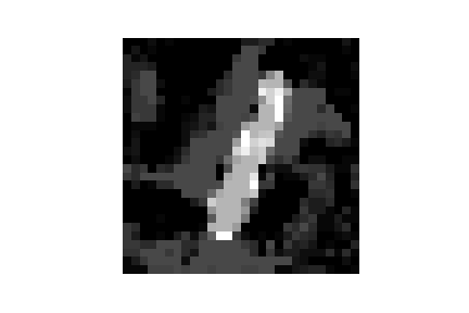
(h) BIM $L_{\infty}$ $1\to 9$

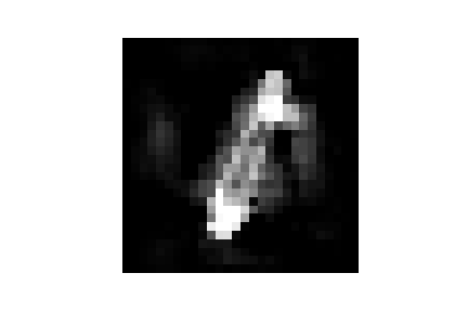
(i) BIM $L_{1}$ $1\to 0$

Figure 3: Adversarial Examples Generated by Attack Algorithms

(a) FGSM 375d $1\to 2$

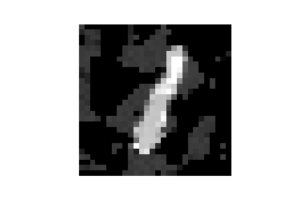
(b) MI 250d $1\to 3$

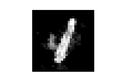
(c) CW2 180d $1\to 4$

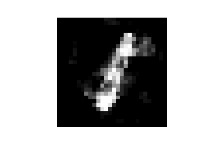
(d) CW2 175d $1\to 5$

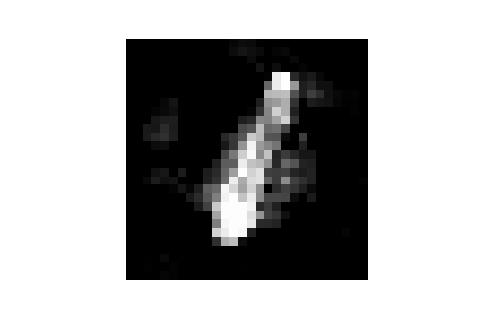
(e) BIM $L_{2}$ 220d $1\to 6$

(f) MI 300d $1\to 7$

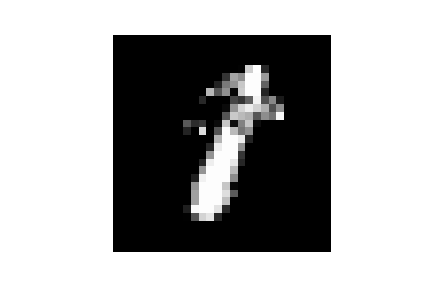
(g) PW 35d $1\to 8$

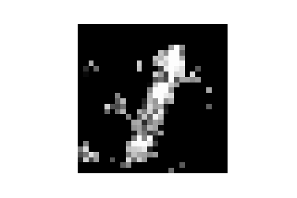
(h) BIM $L_{\infty}$ 110d $1\to 9$

(i) BIM $L_{1}$ 120d $1\to 0$

Figure 4: Adversarial Examples Generated by Sampling in Hyper-Rectangles $R_{k}(t)$

Uncertainty Region Construction

Assume $M_{1}$ is the model under attack. For a given attack algorithm and a object class $t$, $t\neq c$ where $c$ is the true object class of $W$, we combine the adversarial examples $W^{a}$ from both the targeted attack and the untargeted attack, s.t. $M_{1}(W^{a})=t$. We then construct the subspace spanned by $W^{a}$. This step requires an attack algorithm to generate sufficient amount of perturbed images $W^{a}$, at least 80-100 images, given a clean image. Although there are 42 attacks algorithms in Foolbox, most of them cannot satisfy this requirement, including several famous attacks – DeepFool attack [38], L-BFGS attack [57], PGD attack [35] on MNIST. Furthermore we only consider adversarial examples $W^{a}$ in $B(\delta,W)$ with a small $\delta$. Some attacks generate large perturbations that are barely recognizable, such as Spatial Transform Attack [64], Additive Gaussian Noise Attack [50], and Additive Uniform Noise Attack [50]. They are also excluded from the experiments. We only use the attack algorithms listed in Sec. 1.1 in the experiments.

Let $I_{k}(t):=\left\{W^{a}_{k}=(W^{a}_{k,i}):~{}M_{1}(W^{a}_{k})=t,~{}t\neq c\right\}$. $I_{k}(t)$ is the set of adversarial images misclassified to class $t$ by attack algorithm $k$. If $\exists~{}W^{a}_{k,i}\neq W_{i}$, i.e., attack $k$ adds perturbation to the $i$th pixel, we compute the interval size of the $i$th pixel as $s^{t,k}_{i}=max_{I_{k}(t)}(W^{a}_{k,i})-min_{I_{k}(t)}(W^{a}_{k,i})$. Assume $m$ pixels are perturbed by attack $k$. Then the intervals are ranked by interval size as $s^{t,k}_{(1)}\geq s^{t,k}_{(2)}\geq\cdots s^{t,k}_{(m)}$. We construct a hyper-rectangle $R_{k}(t)$ using $b$ largest intervals with $b\leq m$ as

$$R_{k}(t)~{}=~{}[min_{I_{k}(t)}(W^{a}_{k,(1)}),~{}max_{I_{k}(t)}(W^{a}_{k,(1)})]\otimes\cdots\otimes[min_{I_{k}(t)}(W^{a}_{k,(b)}),~{}max_{I_{k}(t)}(W^{a}_{k,(b)})].$$

$R_{k}(t)$ is the subspace based on the adversarial examples generated by attack $k$ and misclassified to class $t$. We choose the number of intervals $b$ that the remaining interval sizes are very small and the perturbations added can be considered as approximately constant.

2.1 MNIST CNN Experiment

Table 5: MLP Mis-classification Rates on Clean MNIST Test Images

$M_{1}$	$M_{2}$	$M_{3}$	$M_{4}$	$M_{5}$
0.0177	0.0178	0.0183	0.0177	0.0176

Table 6: MLP Misclassification Rates in Hyper-Rectangles

	$s_{(i)}$	$M_{1}$	$M_{2}$	$M_{3}$	$M_{4}$	$M_{5}$
CW2 230d $5\to 6$	0.005	0.94	0	0	0	0
CW2 440d $7\to 2$	0.01	0.82	0	0.78	0	0

Table 7: MLP Attack Misclassification Rates

	$M_{1}$	$M_{2}$	$M_{3}$	$M_{4}$	$M_{5}$
CW2 380d $5\to 6$	1	0	0	0	0
CW2 491d $7\to 2$	1	0	0.28	0	0

(a) Clean $5$

(b) CW2 $5\to 6$

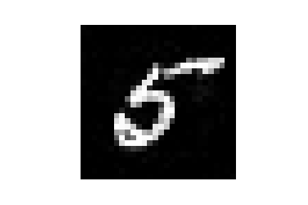
(c) Sampled $5\to 6$

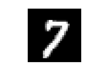
(d) Clean $7$

(e) CW2 $7\to 2$

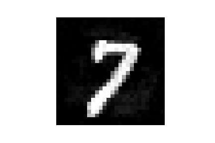
(f) Sampled $7\to 2$

Figure 5: Images for MLP experiment

Here we conduct an experiment with the task to classify MNIST dataset of 10 handwritten digits [37]. MNIST has 60,000 training images and 10,000 test images. Each image has 28x28 gray-scale pixels. Our model is the PyTorch implementation of LeNet [32], which has two convolutional layers. The model structure can be found in [48, 49]. The pixels are rescaled to $[0,1]$ in PyTorch implementation. $W$ is a vectorized MNIST image. We have $W\in[0,1]^{784}$. Table 1 shows the accuracy of 10 trained LeNet models on the MNIST test data using different initial seeds. $M_{1}$ to $M_{10}$ have similar performance.

Intuitively, the ten handwritten digits have distinct features that facilitate the classification task. Hence LeNet can achieve nearly 99% accuracy. We visualize the digits using t-Distributed Stochastic Neighbor Embedding (t-SNE) technique [36], a nonlinear dimension reduction technique. t-SNE uses t distribution to calculate the similarity between two points and can capture the local properties of high dimensional data that lie on lower dimensional manifold. Figure 1 provides a two dimensional projection of the ten digits, based on 2000 sampled images. The digits form tight clusters.

In the experiment, we choose a clean image $W$, and generate adversarial examples using the attack algorithms listed in Section 1.1. We then construct the hyper-rectangles $R_{k}(t)$ that contain the adversarial examples. We have studied many test images and training images, and have obtained similar results. Due to the limited space, here we show the results for a digit 1 from the test data, shown in Figure 2. We run the attacks against $M_{1}$. Table 2 shows the following information.

1. The number of intervals used to construct the hyper-rectangles. For example, CW2 280d $1\to 2$ means $R_{CW2}(2)$ is spanned by the largest 280 intervals.

2. The smallest interval size in $R_{k}(t)$, shown in column $s_{(i)}$. For PW attack, we use [0,1] for the selected pixels, since the measured interval sizes are all close to 1. For all other attacks, the interval size is measured from the added perturbations.

3. We sample 1000 images from each hyper-rectangle $R_{k}(t)$, and report the misclassification rates by $M_{1}$ to $M_{10}$.

The left three columns in Table 3 show the minimum amount of perturbations ($min(||W^{a}-W||_{2})$), the maximum amount of perturbations ($max(||W^{a}-W||_{2})$), and the average amount of perturbations ($mean(||W^{a}-W||_{2})$) of the 1000 sampled images in each hyper-rectangle $R_{k}(t)$. The right three columns in Table 3 show the same information for the adversarial examples generated by the attacks. Figure 3 shows the adversarial examples generated by the attacks. Figure 4 shows the adversarial images generated by sampling in the hyper-rectangles $R_{k}(t)$.

As shown in Table 2, the column of $s_{(i)}$ has the maximum value 0.036. This translates to 12 consecutive integer values on the original 0, 1, …, 255 scale. They are very similar light levels, and can be considered as approximately constant. If we add more dimensions to $R_{k}(t)$, the additional dimensions can be considered as moving the additional pixels to different values. Adding more dimensions do not change the shape and size of $R_{k}(t)$. Instead that moves the hyper-rectangle to a different location, increasing the amount of perturbation and away from the clean image $W$. The hyper-rectangles $R_{k}(t)$ in Table 2 used far fewer pixels than the original attacks. From Table 3, we see that leads to smaller perturbations to create adversarial examples in $R_{k}(t)$. There are more such hyper-rectangles with the same shape and size, as we add more pixels identified by the attacks. Adding more pixels does not necessarily increase the misclassification rates by all DNNs. For Carlini & Wagner $L_{2}$ attack and FGSM, eventually the hyper-rectangle is moved to a place where $M_{1}$ misclassification rate is close to 100% and all other models, $M_{2}$ to $M_{10}$, see near 0% misclassification rate. This is the effect of the optimization approach attacking $M_{1}$.

As highlighted in Table 2, we observe three types of $R_{k}(t)$: (1) the target DNN misclassifies most of the adversarial examples while there exists another DNN which correctly classifies the adversarial examples; (2) the target model correctly classifies the adversarial examples while another DNN misclassifies most of the adversarial examples; (3) the transferable adversarial regions where all DNNs misclassify a significant proportion of the adversarial examples. The highlighted rows in Table 3 shows this phenomenon occurs to attacks adding both small and large perturbations. The first two types of $R_{k}(t)$ belong to DNN uncertainty regions. The existence of DNN uncertainty regions shows transferability of adversarial examples is not universal, contrary to [57, 21, 60]. A better understanding of DNN classification boundary, its uncertainty regions, and transferable adversarial regions, is crucial to improve the robustness of DNN.

Table 4 shows the attacks’ misclassification rates on the 10 LeNet models, and the number of perturbed pixels. Adversarial examples by Carlini & Wagner $L_{2}$ attack are correctly classified by the other 9 models. Compared to Carlini & Wagner $L_{2}$ attack, BIM $L_{1}$, $L_{2}$, $L_{\infty}$, NewtonFool, Moment Iterative attacks perturbed a lot more pixels, between 400 to 600, to generate adversarial examples that cause misclassification from multiple trained DNN models. Notice the hyper-rectangles by our approach, having smaller number of perturbed pixels than the original attacks, can attack several DNNs simultaneously.

Table 8: MobileNet Mis-classification Rates on Clean CIFAR10 Test Images

$M_{1}$	$M_{2}$	$M_{3}$	$M_{4}$	$M_{5}$
0.0767	0.0728	0.0734	0.0727	0.0744

Table 9: MobileNet Attack Misclassification Rates

	$M_{1}$	$M_{2}$	$M_{3}$	$M_{4}$	$M_{5}$
BIM $L_{2}$ 3017d airplane$\to$deer	1	0	0.88	0	0

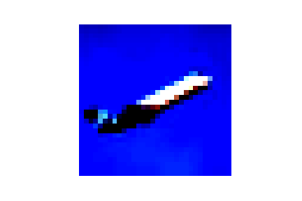
(a) Clean airplane

(b) BIM $L_{2}$ airplane$\to$deer

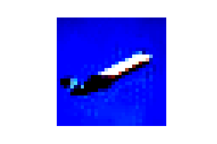
(c) Sampled airplane$\to$deer

Figure 6: Images for MobileNet experiment

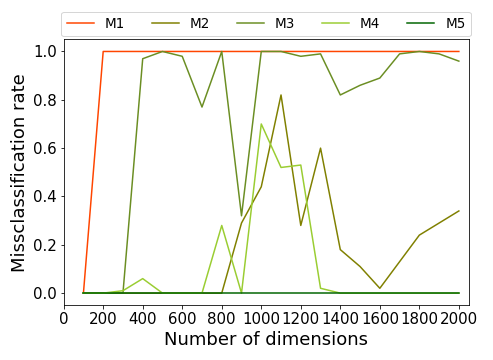
Figure 7: MobileNet misclassification rates in hyper-rectangles

2.2 MNIST MLP Experiment

Here we conduct experiment with a MLP trained on MNIST. It is a fully connected network with 3 layers, 3x512 hidden neurons and ReLU activation. We vary the initial seeds and train 5 MLPs. Table 5 shows the MLP misclassification rates on the clean MNIST test data. They have more consistent performance compared to the 10 CNN models. In the interest of space, here we show two examples, a digit 5 and a digit 7, under Carlini & Wagner $L_{2}$ attack. Table 6 shows the 5 MLPs’ misclassification rates in the hyper-rectangles. Table 7 shows the attacks’ misclassification rates. Figure 5 shows the clean images, adversarial examples generated by Carlini & Wagner $L_{2}$ attack, and adversarial examples generated by sampling from hyper-rectangles. The misclassification rates suggest the hyper-rectangles and the adversarial images generated by Carlini & Wagner $L_{2}$ attack lie in DNN’s uncertainty regions. Again Carlini & Wagner $L_{2}$ attack has great success with the target model $M_{1}$ but can be blocked by the other four MLPs.

Table 10: $L_{2}$ Distance for MLP and MobileNet Experiments

	$L_{2}^{min}$	$L_{2}^{max}$	$\bar{L}_{2}$	$L_{2}^{min}$ Attack	$L_{2}^{max}$ Attack	$\bar{L}_{2}$ Attack
CW2 MLP 230d $5\to 6$	10.47	10.72	10.61	11.06	11.51	11.26
CW2 MLP 440d $7\to 2$	11.18	11.41	11.30	11.51	11.89	11.68
BIM $L_{2}$ 2000d airplane$\to$deer	64.49	67.05	65.88	225	288.32	256.01

2.3 CIFAR10 MobileNet Experiment

We re-train the MobileNet [53] on CIFAR10 [28]. CIFAR10 has 60,000 32x32 color images in 10 classes, with 50,000 as training images and 10,000 as test images. A vectorized CIFAR10 image is in $[0,1]^{3072}$. The dimensionality of a CIFAR10 image is almost 4 times of a MNIST image. MobileNet has an initial convolution layers followed by 19 residual bottleneck layers. [53] shows the network structure. MobileNet has a more complex model structure aiming to reduce memory usage. The misclassification rates of five re-trained MobileNet models on the clean test data by varying initial seeds are in Table 8. For the interest of space, here we show an example with an airplane image under BIM $L_{2}$ attack. The attack success on the five MobileNet models are in Table 9. Note BIM $L_{2}$ attack perturbed 3071 dimensions and left 1 dimension untouched. The images are shown in Figure 6.

Figure 7 shows the misclassification rates as we increase the dimensions of the hyper-rectangle. The largest interval size is 0.2 and the 2000th largest interval size is 0.017. $M1$ misclassifies all the sampled images starting from around 200 perturbed dimensions. $M5$ correctly classifies all the sampled images. We see $M2$ and $M4$ misclassification rates increase as more effective dimensions are included, then decrease as we include additional irrelevant dimensions. The 2000-dimensional hyper-rectangle is a MobileNet uncertainty region. As noted in [21], the direction of adversarial perturbation is important. Adversarial examples cannot be generated by randomly sampling in 3072 dimensional $\delta-$ neighborhood $B(\delta,W)$. The lower dimensional hyper-rectangles $R_{k}(t)$ containing infinitely many adversarial examples are discovered through optimization approach, i.e., the attack algorithms. Table 10 shows that the sampled adversarial images from the hyper-rectangle have much smaller perturbations than the original attack on CIFAR10.

Strategy for Robust Classification

Our experiments confirm that transferability of adversarial examples is not universal. Notice all the trained DNNs achieve the same level of accuracy over the clean test images, but their performance vary a lot over the hyper-rectangles. Although in some hyper-rectangles, all the trained models misclassify a large portions of the sampled adversarial images, in uncertainty regions, there exist at least one DNN that can correctly classify all the adversarial images. This naturally leads to a strategy to make robust decision. If at least one DNN assigns a label that is different from another DNN, the image triggers an alert and requires additional screening, either involving a human operator or alternative classifiers. This strategy will significantly improve the accuracy over the adversarial examples in DNN uncertainty regions, but won’t solve the problem for transferable adversarial examples. Although an ensemble can mitigate many attacks, based on Tables 4, 7, 9, unfortunately an ensemble of DNNs may not achieve the desirable accuracy over uncertainty regions. There is no guarantee about the number of DNNs that can make correct decision over each uncertainty region. We also need to understand how to measure the size of DNN uncertainty regions vs. DNN transferable adversarial regions. We leave it to the future work.

3 Generalization Error and Adversarial Examples

The classification accuracy on test data is often used to measure a classifier’s performance. However, in [40], the authors argued the test data accuracy is not the most appropriate performance measure, because the variability due to the randomness of the training data needs to be taken into consideration, besides those due to the test data. Let $Z=(W,Y)$ denote a sample, where $W\in[0,1]^{h}$ is the $h-$dimensional vectorized image features and $Y\in\{1,\cdots,c\}$ is the true object class. $Z$ is generated independently and identically from a distribution $F$ over $[0,1]^{h}$. We denote a training dataset with $n$ sample points by $D_{n}=(Z_{1},\cdots,Z_{n})$. [40] defined generalization error as $E(loss_{M}(D_{n},Z_{n+1}))$, where $Z_{n+1}$ is a test sample, and $loss_{M}()$ is the loss of applying a classifier $M$ trained on $D_{n}$ to $Z_{n+1}$. If $loss_{M}()$ is a 0-1 loss, the generalization error is defined as the error probability $P(M(W)\neq Y)$ in [27]. Another definition of generalization error involves the empirical error on the training data. Let $\hat{loss}_{M}(D_{n})=\frac{1}{n}\sum_{1}^{n}loss(Z_{i})$ be the empirical risk estimated from the training data $D_{n}$. [66] defined generalization error as $E(loss_{M}(D_{n},Z_{n+1}))-\hat{loss}_{M}(D_{n})$, which is widely used in many recent papers to establish DNN theoretical guarantees.

There is an extensive literature on theoretical generalization error bound, for different type of classifiers including DNN. [40] suggested the generalization error can be estimated through cross validation. Experiments were conducted on least square linear regression, regression tree, classification tree and nearest neighbor classifier. They built normal confidence interval or confidence intervals based on Student’s t distribution for generalization error. Subsequently, [27] obtained generalization error bound based on the disagreement probability between classifiers, and computed the generalization error bound of SVM on MNIST data. Generalization error bound for DNN is proven to be $O(\frac{c(depth,width)}{\sqrt{n}})$, where $c(depth,width)$ refers to a constant based on the width and depth of a DNN model, e.g., in [65, 4, 3, 19, 33, 41, 42, 55].

We observe there is a discrepancy between the theoretically proven generalization error bound for DNN and the existence of adversarial examples. Following the theory, the error on test data should decrease to 0 at a rate proportional to $n^{-1/2}$ where $n$ is the training sample size. But given a clean image, we show there exists infinitely many adversarial images in $B(\delta,W)$ for different network structures and datasets. Adversarial examples exist for large DNN models trained on ImageNet with millions of training data, where the theoretical asymptotic behavior of DNN should already kick in. Here we offer an explanation for why this happens. Let $L_{r}$ be a $r-$dimensional region in $[0,1]^{h}$ with $r<h$. Let $\mathcal{L}=\cup_{i=1}^{\infty}L_{r_{i}}$ be the union of countably infinite non-overlapping lower dimensional regions $L_{r_{i}}$ in $[0,1]^{h}$ with all $r_{i}<h$.

Theorem 1.

Let $M_{1}$ and $M_{2}$ be two DNN models trained on $D_{n}$. Assume $\forall~{}W\in[0,1]^{h}-\mathcal{L}$, $M_{1}(W)=M_{2}(W)$. And assume $\exists~{}W\in\mathcal{L}$, s.t. $M_{1}(W)\neq M_{2}(W)$. We have

$$E(loss_{M_{1}}(D_{n},Z_{n+1}))=E(loss_{M_{2}}(D_{n},Z_{n+1})).$$

Proof.

For any continuous distribution $F$ on $[0,1]^{h}$, $F(\mathcal{L})=0$, i.e., the lower dimensional region $\mathcal{L}$ has 0 probability mass. For two functions that differ only on 0 probability region, we have

$$E(loss_{M_{1}}(D_{n},Z_{n+1}))=E(loss_{M_{2}}(D_{n},Z_{n+1})).$$

∎

Corollary 1.1.

There exist $M_{1}$ and $M_{2}$ s.t.

$$E(loss_{M_{1}}(D_{n},Z_{n+1}))-\hat{loss}_{M_{1}}(D_{n})=E(loss_{M_{2}}(D_{n},Z_{n+1}))-\hat{loss}_{M_{2}}(D_{n}).$$

Proof.

Corollary 1 in [66] states there exists neural networks with ReLU activation, depth $g$, width $O(n/g)$ and weights $O(n+h)$, that can fit exactly any function on $D_{n}$ in $h-$dimensional space. Assume $M_{1}$ and $M_{2}$ are such models trained on $D_{n}$. $\hat{loss}_{M_{1}}(D_{n})=\hat{loss}_{M_{2}}(D_{n})=0$. By only changing initial seeds during training, $M_{1}$ and $M_{2}$ satisfy the conditions in Theorem 1. Consequently we have

$$E(loss_{M_{1}}(D_{n},Z_{n+1}))-\hat{loss}_{M_{1}}(D_{n})=E(loss_{M_{2}}(D_{n},Z_{n+1}))-\hat{loss}_{M_{2}}(D_{n}).$$

∎

Remark

The volume of a $h-$dimensional $B(\delta,W)$ is $|B(\delta,W)|=\frac{\pi^{h/2}}{\Gamma(1+h/2)}\delta^{h}$. The volume of the feature space $[0,1]^{h}$ is 1. Hence for a fixed $\delta$ and $h$, there are only finite number of non-overlapping $\delta$ balls in the feature space $[0,1]^{h}$. As $h\longrightarrow\infty$, we have $|B(\delta,W)|\longrightarrow 0$. Hence the feature space for higher resolution color images can contain increasingly more clean images. The existing attack algorithms collectively identify finite number of lower dimensional regions in $B(\delta,W)$ for each clean image. Theorem 1 means $E(loss_{M_{1}}(D_{n},Z_{n+1}))$ cannot tell the difference between a trained classifier that assign correct labels to all sample points in $B(\delta,W)$ and a different classifier that assign wrong labels only to sample points in finite or countably infinite lower dimensional bounded regions. Hence the generalization error definition and the subsequently proven large sample property of DNN based on generalization error cannot adequately describe the phenomenon of adversarial examples. We need new theory to measure DNN robustness.

4 Conclusion

Limitation of our work is that we rely on the existing attack algorithms to identify these hyper-rectangles. Also our approach works with low resolution images. Our conjecture is for high resolution images, adversarial examples lie in bounded regions on lower dimensional manifold. Again we leave it to the future work to capture the DNN classification boundary in much higher dimensional feature space.

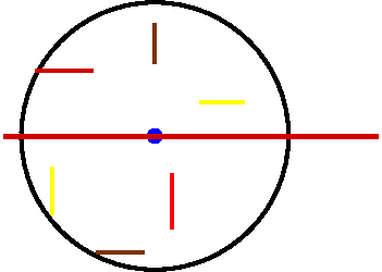
Figure 8: Conceptual Plot of DNN Classification Boundary in $B(\delta)$

We use Figure 8 to show a conceptual plot of DNN classification boundary in the neighborhood $B(\delta,W)$. For the digit 1, let $\delta=6$. The blue dot in the center is the clean image. Inside the black circle, the image samples can be correctly recognized by people as 1, but there exists adversarial examples causing misclassification errors. The hyper-rectangles are lower dimensional small “cracks” inside the circle. There are three types of such “cracks”, illustrated using three different colors.

1. $W^{a}$s are misclassified by $M_{1}$ but can be correctly classified by some other model $M_{j}$;

2. $W^{a}$s are correctly classified by $M_{1}$ but misclassified by some $M_{j}$;

3. $W^{a}$s are misclassified by all the models, $M_{1}$ to $M_{10}$.

Type 1 and 2 hyper-rectangles belong to DNN uncertainty regions. Type 3 hyper-rectangles are the transferable adversarial regions which are more difficult to handle. We conclude that the adversarial examples stem from a structure problem of DNN. DNN’s classification boundary is unlike that of any other classifier. Current defense strategies do not address this structural problem. We also need new theory to describe the phenomenon of adversarial examples and measure the robustness of DNN.

References

- [1] Adadi, A. and Berrada, M. Peeking inside the black-box: A survey on Explainable Artificial Intelligence (XAI). IEEE Access, 6, 52138-52160, (2018)
- [2] Akhtar, N. and Mian, A. Threat of adversarial attacks on deep learning in computer vision: A survey. IEEE Access, 6, 14410-14430, (2018).
- [3] Bartlett, P. L. The sample complexity of pattern classification with neural networks: The size of the weights is more important than the size of the network. I͡EEE Transactions on Information Theory, 44(2), 525–536. (1998).
- [4] Bartlett, P. L., Foster, D. J., and Telgarsky, M. J. Spectrally-normalized margin bounds for neural networks. Advances in neural information processing systems, 6241–6250. Long Beach, CA. (2017)
- [5] Behzadan, V. and Munir, A. Vulnerability of deep reinforcement learning to policy induction attacks. In International Conference on Machine Learning and Data Mining in Pattern Recognition, 262-275, (2017).
- [6] Brendel, W., Rauber, J. and Bethge, M. Decision-Based Adversarial Attacks: Reliable Attacks Against Black-Box Machine Learning Models. In International Conference on Learning Representations, 1-11, (2018)
- [7] Biggio, B. and Roli, F. Wild patterns: Ten years after the rise of adversarial machine learning. Pattern Recognition, 84, 317-331, (2018).
- [8] Box, G.E. and Draper, N.R. A basis for the selection of a response surface design. Journal of the American Statistical Association, 54(287), 622-654, (1959).
- [9] Box, G.E. and Draper, N.R. The choice of a second order rotatable design. Biometrika, 335-352, (1963).
- [10] Box, G.E. and Draper, N.R. Robust designs. Biometrika, 62(2), 347-352, (1975).
- [11] Carlini, N. and Wagner, D. Towards evaluating the robustness of neural networks. In 2017 IEEE Symposium on Security and Privacy, 39-57, (2017).
- [12] Crecchi, F., Bacciu, D. and Biggio, B. Detecting adversarial examples through nonlinear dimensionality reduction. In 27th European Symposium on Artificial Neural Networks, Computational Intelligence and Machine Learning (ESANN), 483-488, (2019).
- [13] Deka, S.A., Stipanović, D.M. and Tomlin, C.J.Dynamically Computing Adversarial Perturbations for Recurrent Neural Networks. arXiv preprint arXiv:2009.02874, (2020).
- [14] Dong, Y., Liao, F., Pang, T., Su, H., Zhu, J., Hu, X. and Li, J., 2018. Boosting adversarial attacks with momentum. In Proceedings of the IEEE conference on computer vision and pattern recognition, 9185-9193, (2018).
- [15] Dosilovic, F.K., Brcic, M. and Hlupic, N. Explainable artificial intelligence: A survey. In the 41st International convention on information and communication technology, electronics and microelectronics (MIPRO), 0210-0215, (2018).
- [16] Foolbox Native: Fast adversarial attacks to benchmark the robustness of machine learning models in PyTorch, TensorFlow, and JAX, https://github.com/bethgelab/foolbox (last accessed on 12/04/2020).
- [17] Rauber, J., Brendel, W. and Bethge, M. Foolbox: A python toolbox to benchmark the robustness of machine learning models. arXiv preprint arXiv:1707.04131, (2017).
- [18] Gao, J., Lanchantin, J., Soffa, M.L. and Qi, Y. Black-box generation of adversarial text sequences to evade deep learning classifiers. In 2018 IEEE Security and Privacy Workshops (SPW), 50-56, (2018).
- [19] Golowich, N., Rakhlin, A., and Shamir, O. Size-independent sample complexity of neural networks. In Proceedings of the 31st Conference on Learning Theory. Vancouver, BC, Canada. (2018).
- [20] Goodfellow, I., Bengio, Y., Courville, A. and Bengio, Y. Deep learning. Cambridge: MIT press, (2016).
- [21] Goodfellow, I.J., Shlens, J. and Szegedy, C. Explaining and harnessing adversarial examples. In International Conference on Learning Representations (ICLR), 1-11, (2015).
- [22] Huang, S., Papernot, N., Goodfellow, I., Duan, Y. and Abbeel, P. Adversarial attacks on neural network policies. arXiv preprint arXiv:1702.02284, (2017).
- [23] Huber, P.J. Robust statistics (Vol. 523). John Wiley & Sons, (2004).
- [24] Huo, L.Z. and Tang, P. A graph-based active learning method for classification of remote sensing images. International Journal of Wavelets, Multiresolution and Information Processing, 16(04), p.1850023, (2018)
- [25] Jakubovitz, D., Giryes, R., and Rodrigues, M. R. Generalization error in deep learning. In Compressed Sensing and Its Applications, 153–193. (2019)
- [26] Jang, U., Wu, X. and Jha, S. Objective metrics and gradient descent algorithms for adversarial examples in machine learning. In Proceedings of the 33rd Annual Computer Security Applications Conference, 262-277, (2017).
- [27] Kaariainen M. Generalization Error Bounds Using Unlabeled Data. In: International Conference on Computational Learning Theory (COLT). Lecture Notes in Computer Science, vol 3559: 127–142 (2005)
- [28] Alex Krizhevsky. Learning multiple layers of features fromtiny images. University of Toronto, 05 2012.
- [29] Krizhevsky, A., Sutskever, I. and Hinton, G.E. January. ImageNet Classification with Deep Convolutional Neural Networks. In Neural Information Processing Systems (NIPS), 1-9, (2012).
- [30] Khuri, A.I. and Mukhopadhyay, S. Response surface methodology. Wiley Interdisciplinary Reviews: Computational Statistics, 2(2), 128-149, (2010).
- [31] Kurakin, A., Goodfellow, I. and Bengio, S. Adversarial examples in the physical world. arXiv preprint arXiv:1607.02533, (2016).
- [32] LeCun, Y., Bottou, L., Bengio, Y. and Haffner, P.Gradient-based learning applied to document recognition. Proceedings of the IEEE, 86(11), 2278-2324, (1998).
- [33] Li, X., Lu, J., Wang, Z., Haupt, J., and Zhao, T. On tighter generalization bound for deep neural networks: CNNs, ResNets, and beyond. arXiv preprint arXiv:1806.05159. (2018).
- [34] Lin, Y.C., Hong, Z.W., Liao, Y.H., Shih, M.L., Liu, M.Y. and Sun, M. Tactics of adversarial attack on deep reinforcement learning agents. In Proceedings of the 26th International Joint Conference on Artificial Intelligence, 3756-3762, (2017).
- [35] Madry, A., Makelov, A., Schmidt, L., Tsipras, D. and Vladu, A. Towards Deep Learning Models Resistant to Adversarial Attacks. In International Conference on Learning Representations (ICLR), 1-10, (2018).
- [36] Maaten, L.V.D. and Hinton, G. Visualizing data using t-SNE. Journal of machine learning research, 9(Nov), 2579-2605, (2008).
- [37] Modified National Institute of Standards and Technology (MNIST) dataset. http://yann.lecun.com/exdb/mnist/ (last accessed on Dec. 07, 2020).
- [38] Moosavi-Dezfooli, S.M., Fawzi, A. and Frossard, P. Deepfool: a simple and accurate method to fool deep neural networks. In Proceedings of the IEEE conference on computer vision and pattern recognition (CVPR), 2574-2582, (2016).
- [39] Myers, R.H., Montgomery, D.C. and Anderson-Cook, C.M. Response surface methodology: process and product optimization using designed experiments. John Wiley & Sons. (2016)
- [40] Nadeau, C. and Bengio, Y. Inference for the generalization error. Machine learning, 52(3), 239-281, (2003).
- [41] Neyshabur, B., Tomioka, R., and Srebro, N. Norm-based capacity control in neural networks. In Conference on Learning Theory, 1376–1401. (2015).
- [42] Neyshabur, B., Bhojanapalli, S., and Srebro, N. A PAC-Bayesian approach to spectrally-normalized margin bounds for neural networks. In International Conference on Learning Representations. Vancouver, BC, Canada. (2018).
- [43] Papernot, N., McDaniel, P., Swami, A. and Harang, R. Crafting adversarial input sequences for recurrent neural networks. In IEEE Military Communications Conference (MILCOM), 49-54, (2016).
- [44] Papernot, N., McDaniel, P. and Goodfellow, I. Transferability in machine learning: from phenomena to black-box attacks using adversarial samples. arXiv preprint arXiv:1605.07277, (2016).
- [45] Patra, S. and Bruzzone, L. A batch-mode active learning technique based on multiple uncertainty for SVM classifier. IEEE Geoscience and Remote Sensing Letters, 9(3), 497-501, (2011).
- [46] Pattanaik, A., Tang, Z., Liu, S., Bommannan, G. and Chowdhary, G. Robust Deep Reinforcement Learning with Adversarial Attacks. In Proceedings of the 17th International Conference on Autonomous Agents and MultiAgent Systems, 2040-2042, (2018).
- [47] Portnoy, S. and He, X. A robust journey in the new millennium. Journal of the American Statistical Association, 95(452), 1331-1335, (2000).
- [48] PyTorch: Adversarial Example Generation, https://pytorch.org/tutorials/beginner/fgsm_tutorial.html
- [49] PyTorch Tutorial on Neural Network: https://pytorch.org/tutorials/beginner/blitz/neural_networks_tutorial.html
- [50] Rauber, J., Brendel, W. and Bethge, M. Foolbox: A python toolbox to benchmark the robustness of machine learning models. arXiv preprint arXiv:1707.04131 (2017).
- [51] Rosenberg, I., Shabtai, A., Elovici, Y. and Rokach, L. Query-Efficient Black-Box Attack Against Sequence-Based Malware Classifiers. arXiv preprint arXiv:1804.08778, (2018).
- [52] Rosenberg, I., Shabtai, A., Rokach, L. and Elovici, Y. Generic black-box end-to-end attack against state of the art API call based malware classifiers. In International Symposium on Research in Attacks, Intrusions, and Defenses, 490-510, (2018).
- [53] Sandler, M., Howard, A., Zhu, M., Zhmoginov, A., and Chen, L. C. Mobilenetv2: Inverted residuals and linear bottlenecks. In Proceedings of the IEEE conference on computer vision and pattern recognition, 4510–4520, 2018.
- [54] Sokolic, J., Giryes, R., Sapiro, G., and Rodrigues, M. R. D. Generalization Error of Invariant Classifiers. In Proceedings of the 20th International Conference on Artificial Intelligence and Statistics (AISTATS), PMLR 54:1094-1103, (2017)
- [55] Sun, S., Chen, W., Wang, L., Liu, X., and Liu, T.-Y. On the depth of deep neural networks: A theoretical view. In AAAI, Phoenix, Arizona, 2066–2072. (2016).
- [56] Suzuki, T. (2018, March). Fast generalization error bound of deep learning from a kernel perspective. In Proceedings of the 21st International Conference on Artificial Intelligence and Statistics (AISTATS), PMLR 84: 1397-1406. (2018)
- [57] Szegedy, C., Zaremba, W., Sutskever, I., Estrach, J.B., Erhan, D., Goodfellow, I. and Fergus, R. Intriguing properties of neural networks. In 2nd International Conference on Learning Representations (ICLR), 1-10, (2014).
- [58] Tang, X., Li, Y., Sun, Y., Yao, H., Mitra, P. and Wang, S. Transferring Robustness for Graph Neural Network Against Poisoning Attacks. In Proceedings of the 13th International Conference on Web Search and Data Mining, 600-608, (2020).
- [59] Terada, Y., and Hirose, R. Fast generalization error bound of deep learning without scale invariance of activation functions. Neural Networks, 129, 344-358. (2020)
- [60] Tramer, F., Papernot, N., Goodfellow, I., Boneh, D., and McDaniel, P. The space of transferable adversarial examples. arXiv preprint arXiv:1704.03453, 1–15, (2017)
- [61] Tuia, D., Ratle, F., Pacifici, F., Kanevski, M.F. and Emery, W.J. Active learning methods for remote sensing image classification. IEEE Transactions on Geoscience and Remote Sensing, 47(7), 2218-2232, (2009)
- [62] Voichita, C., Khatri, P. and Draghici, S. Identifying uncertainty regions in support vector machines using geometric margin and convex hulls. In 2008 IEEE International Joint Conference on Neural Networks (IEEE World Congress on Computational Intelligence), 3319-3324, (2008).
- [63] Xi, B., Adversarial machine learning for cybersecurity and computer vision: Current developments and challenges. Wiley Interdisciplinary Reviews: Computational Statistics, pp. e1511, (2020).
- [64] Xiao, C., Zhu, J.Y., Li, B., He, W., Liu, M. and Song, D. Spatially transformed adversarial examples. In 6th International Conference on Learning Representations (ICLR), 1-10, (2018).
- [65] Xu, Y. and Wang, X. Weight normalized deep neural networks. Stat, 10(1), e344, 1–9. (2021).
- [66] Zhang, C., Bengio, S., Hardt, M., Recht, B., and Vinyals, O. Understanding deep learning requires rethinking generalization. In 5th International Conference on Learning Representations (ICLR), 1–15, (2017)
- [67] Zügner, D., Akbarnejad, A. and Günnemann, S. Adversarial attacks on neural networks for graph data. In Proceedings of the 24th ACM SIGKDD International Conference on Knowledge Discovery & Data Mining, 2847-2856, (2018).