Gauge Enhanced Quantum Criticality
Beyond the Standard Model

Juven Wang¹   Yi-Zhuang You<sup>2

1</sup>Center of Mathematical Sciences and Applications, Harvard University, Cambridge, MA 02138, USA
²Department of Physics, University of California, San Diego, CA 92093, USA

Standard lore ritualizes our quantum vacuum in the 4-dimensional spacetime (4d) governed by one of the candidate Standard Models (SMs), while lifting towards some Grand Unification-like structure (GUT) at higher energy scales. In contrast, in our work, we introduce an alternative view that the SM is a low energy quantum vacuum arising from various neighbor vacua competition in an immense quantum phase diagram. In general, we can regard the SM arising near the gapless quantum criticality (either critical points or critical regions) between the competing neighbor vacua. In particular detail, we demonstrate how the $su(3)\times su(2)\times u(1)$ SM with 16n Weyl fermions arises near the quantum criticality between the GUT competition of Georgi-Glashow (GG) $su(5)$ and Pati-Salam (PS) $su(4)\times su(2)\times su(2)$. We propose two enveloping toy models. Model I is the conventional $so(10)$ GUT with a Spin(10) gauge group plus GUT-Higgs potential inducing various Higgs transitions. Model II modifies Model I by adding a new 4d discrete torsion class of Wess-Zumino-Witten-like term built from GUT-Higgs field (that matches a nonperturbative global mixed gauge-gravity anomaly captured by a 5d invertible topological field theory $w_{2}w_{3}(TM)=w_{2}w_{3}(V_{\rm SO(10)})$), which manifests a Beyond-Landau-Ginzburg quantum criticality between GG and PS models, with extra Beyond-the-Standard-Model (BSM) excitations emerging near a quantum critical region. If the internal symmetries were treated as global symmetries (or weakly coupled to probe background fields), we show an analogous gapless 4d deconfined quantum criticality with new BSM fractionalized fragmentary excitations of Color-Flavor separation, and gauge enhancement including a Dark Gauge force sector, altogether requiring a double fermionic Spin structure named DSpin. If the internal symmetries are dynamically gauged (as they are in our quantum vacuum), we show the 4d criticality as a boundary criticality such that only appropriately gauge enhanced dynamical $so(10)$ GUT gauge fields can propagate into an extra-dimensional 5d bulk. The phenomena may be regarded as SM deformation or “morphogenesis.”

“The Valley Spirit (Void Spirit) never dies;
It is named the Mysterious Female.
And the gateway of the Mysterious Female;
It is called the root of Heaven and Earth.
Dimly visible, it is there within us all the while;
Draw upon it as you will, yet use will never drain it.”

Laozi (B.C. 600) - Dao De Jing - an excerpt

1 Introduction, Motivation, and Summary

It is a common ritual practice in high-energy physics (HEP) to regards our quantum vacuum in the 4-dimensional spacetime (denoted as 4d or 3+1d) governed by one of the candidate $su(3)\times su(2)\times u(1)$ Standard Models (SMs) [1, 2, 3, 4] as a quantum field theory (QFT) and an effective field theory (EFT) suitable below a certain energy scale, while lifting towards one of some Grand Unification-like structure (GUT) [5, 6, 7] or String Theory at higher energy scales, see Fig. 1 (a). Although many non-supersymmetric GUT models had been ruled out by experiments due to no evidence yet on the predicted proton decay (proton lifetime $>10^{34}$ years) [8], many physicists still speculate that GUT plays a certain crucial role in a higher energy unification [9]. How can we remedy the conventional GUTs other than seeking for their supersymmetry (SUSY) variants or String Theory modifications at higher energy?

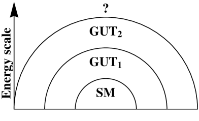
(a) (b)

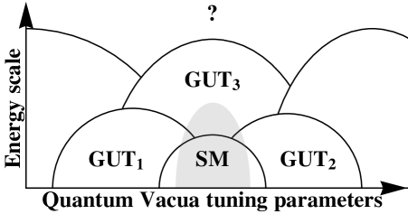
Figure 1: (a) Standard lore seeks for a single unified dynamically gauged internal symmetry at high energy. One probes the shorter distance and higher energy scales to look for the GUT, SUSY, or String Theory evidence. The vertical axis shows an energy scale, while the horizontal axis plays no physical role. (b) We propose an alternative view: SM is just one of many possible low energy phases of the quantum vacua of our universe. By introducing a horizontal axis that represent many possible quantum vacua tuning parameters, we can show that SM phase can tune to other GUT phases, even at a fix energy scale (without the necessity to go to higher energy) and at zero temperature. SM arises near the gapless quantum critical region (shown as the gray area).

To address the above question, we propose to seek for a new viewpoint. In our present work, instead of viewing GUT only as some higher-energy theory of SM, we suggest that various GUTs may be neighbor quantum vacua next to SM in an immense quantum phase diagram shown schematically in Fig. 1 (b), with an underlying larger quantum vacua tuning parameter space (i.e., the horizontal axis in Fig. 1 (b), 2 and 3). We provide two explicit Toy Models in Fig. 2 and Fig. 3: SM arises near the gapless quantum critical point (for Fig. 2) or critical region (gray area for Fig. 3) between the competing neighbor GUT vacua. Readers may be puzzled: What precisely can be the quantum vacua tuning parameters? What can we gain from this viewpoint? What are the motivations? Let us address these issues one by one.

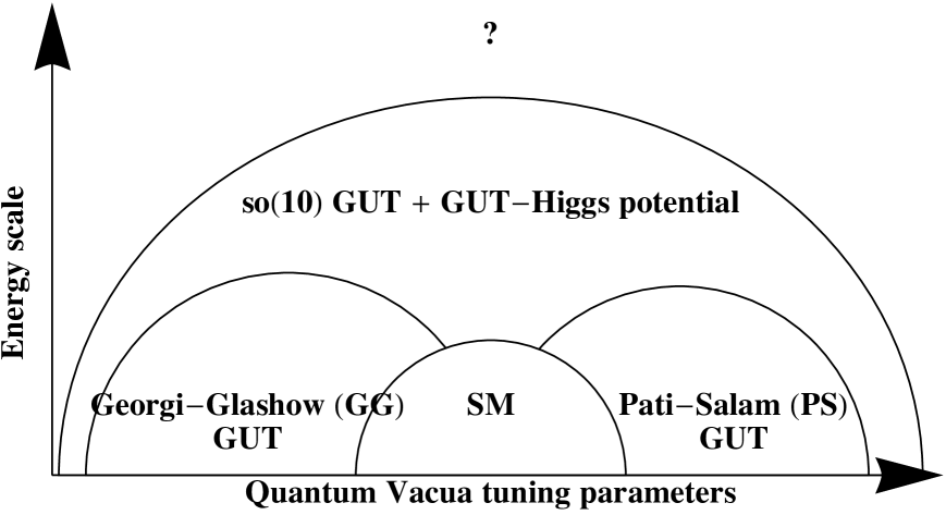
Figure 2: Schematic phases for the Toy Model I: The parent EFT is the conventional $so(10)$ GUT with a Spin(10) gauge group plus GUT-Higgs potential inducing various Higgs transitions to GG, PS, or SM.

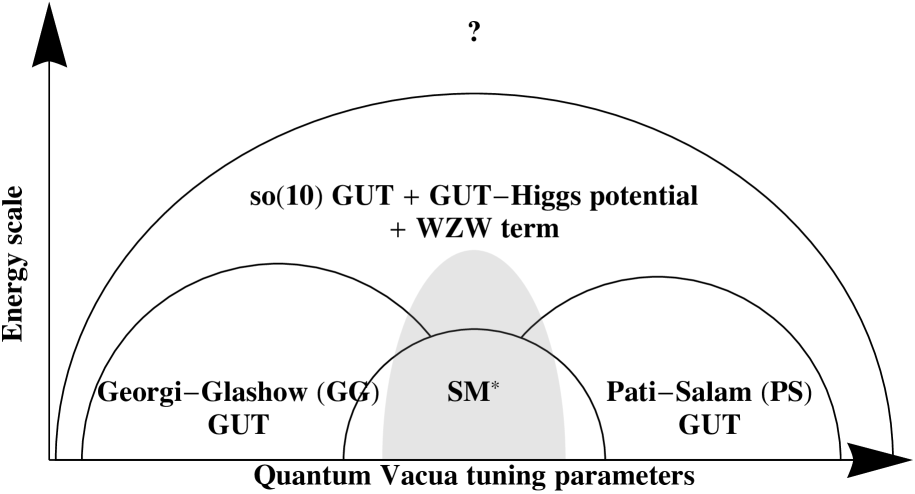
Figure 3: Schematic phases for the Toy Model II: The parent EFT is a modified $so(10)$ GUT with a Spin(10) gauge group, plus not only a GUT-Higgs potential but also a new 4d discrete torsion class of Wess-Zumino-Witten-like (WZW) term built from GUT-Higgs fields that saturates a nonperturbative global mixed gauge-gravity anomaly captured by a 5d invertible topological field theory $w_{2}w_{3}(TM)=w_{2}w_{3}(V_{\rm SO(10)})$, which manifests a Beyond-Landau-Ginzburg quantum critical region (shown in a gray area) between GG and PS models, with extra Beyond-the-Standard-Model (BSM) excitations emerging near the quantum criticality. The SM + BSM physics is denoted as SM^∗.

• Quantum vacua tuning parameters can be as familiarly simple as the tuning of the GUT-Higgs potential $(\Big{(}r_{{\mathbf{R}}}(\Phi_{\mathbf{R}})^{2}+\lambda_{{\mathbf{R}}}(\Phi_{{\mathbf{R}}})^{4}\Big{)})$ of some GUT-Higgs field $\Phi_{\mathbf{R}}$ that can induce a Higgs condensation phase transition via tuning from $r_{{\mathbf{R}}}>0$ to $r_{{\mathbf{R}}}<0$. The quantum vacua tuning parameters can be those triggering a scalar condensation $\langle\Phi_{\mathbf{R}}\rangle\neq 0$ in the $r_{{\mathbf{R}}}<0$ region. The possibility to access the GUT vacua from the SM vacuum by tuning certain model parameters has been largely overlooked in the existing literature, because some of these tuning parameters appear to be perturbatively irrelevant at the SM fixed point. A key proposal of this work is to investigate the non-perturbative effect of these tuning parameters in driving quantum phase transitions from the SM phase to adjacent GUT phases.

• Deformation class of QFT: Given the importance of symmetry and its associated ’t Hooft anomaly of QFT, Seiberg [11] and others conjectured that seemly different $d$d QFTs within the same symmetry $G$ and same ’t Hooft anomaly ${\mathbf{Z}}_{d+1}$ of symmetry $G$ [14] can indeed be deformed to each other via adding degrees of freedom at short distances that preserve the same symmetry and that maintain the same overall anomaly. Namely, the whole system allows all symmetric interactions between the original QFT and any new symmetric QFTs brought down from high energy. This organization principle that connects a large class of QFTs together within the same data $(G,{\mathbf{Z}}_{d+1})$ via any symmetric deformation (possibly with discontinuous or continuous quantum phase transitions [10] between different phases) is called the deformation class of QFTs in $d$d [11], which is indeed controlled by the cobordism or deformation class of invertible topological quantum field theory ${\mathbf{Z}}_{d+1}$ in $d+1$d [15]. One can further define the deformation class for 4d SM [16].

  As we will see, our viewpoint in Fig. 1 (b) (also in Fig. 2 and Fig. 3) is not only compatible with this symmetric deformation class of QFT [11], but also that we allow symmetry-breaking deformations, along the quantum vacua tuning parameter space. We may refer to all these deformations of the SM to other neighbor vacua as “morphogenesis” of the SM.

• Proton decay: The aforementioned issue of GUT proton decay may be resolved in our framework by two ways. First, the change of viewpoint — instead of looking for GUT proton decay in our vacuum (or in a higher energy GUT along the vertical axis, as in Fig. 1), we may look for GUT proton decay by first moving to the appropriate quantum vacuum along the horizontal axis in Fig. 1 (b) that already lives this specific GUT. Second, a modified parent EFT that controls all possible deformation of SM in the phase diagram may give rise to a different proton decay rate. The experimental bound on proton decay rate only rules out the possibility to access non-supersymetic GUT phases from the SM phases by thermal phase transitions (i.e. by raising the energy or temperature scales), but it does not say anything about accessing these GUT phases by quantum phase transitions (by tuning parameters near ground states at low-energy). This work exactly focuses on the later possibility of quantum phase transitions among the SM and GUTs.

The above three arguments summarize the motivation and philosophy behind our viewpoint. Namely, in our present work, we initiate and introduce an alternative complementary perspective — we propose that the SM vacuum can be a low energy quantum vacuum arising from the quantum competition of various neighbor GUT vacua in a quantum phase diagram. SM is just one possible phase allowed by the deformation class of SM [16]. Let us list down some key results of our work:

• In general, we propose that the SM may arise as one adjacent phase from the vicinity of gapless quantum criticality (either a critical point for Model I in Fig. 2, or a critical region for Model II in Fig. 3) between the competing neighbor GUT vacua.

• In particular, we demonstrate how the $su(3)\times su(2)\times u(1)$ SM [1, 2, 3, 4] with 16n Weyl fermions (Fig. 4) could emerge near the quantum criticality between two neighbor vacua of Georgi-Glashow $su(5)$ model (GG) [5] (Fig. 5) and Pati-Salam $su(4)\times su(2)\times su(2)$ model (PS) [6] (Fig. 6), which represents two distinct Higgs phases of the further unified $so(10)$ GUT (with a Spin(10) gauge group).

• We propose two explicit Toy Models. The two models are differed by whether they can carry a 4d nonperturbative global anomaly of mixed gauge-gravitational (i.e., gauge-diffeomorphism) probes, captured by a 5d invertible topological quantum field theory (TQFT):

  $$(-1)^{\int{\rm p}\;w_{2}w_{3}(TM)}=(-1)^{\int{\rm p}\;w_{2}w_{3}(V_{{\rm SO}(10)})}\text{ with ${\rm p}\in\{0,1\}=\mathbb{Z}_{2}$. }$$ (1.1)

  Toy Model I as the ${\rm p}=0$ class without $w_{2}w_{3}$ anomaly: Its parent EFT is the conventional $so(10)$ GUT with a Spin(10) gauge group [7] plus a GUT-Higgs potential inducing various Higgs transitions to GG, PS, or SM, schematically shown in Fig. 2. The first model has no $w_{2}w_{3}$ or any other anomaly within the Spin(10).

  Toy Model II as the ${\rm p}=1$ class with $w_{2}w_{3}$ anomaly and WZW term: To introduce non-trivial competitions between GG and PS phases, we consider a new parent EFT of a modified $so(10)$ GUT with a Spin(10) gauge group, which includes not only the familiar $so(10)$ GUT plus a GUT-Higgs potential, but also a new extra 4d discrete torsion class of Wess-Zumino-Witten-like (WZW) term that saturates a mod-2 class $w_{2}w_{3}$ anomaly within the Spin(10).

  The WZW term introduces nonperturbative interaction effects between different GUT-Higgs fields, which cause a substantial change of the deformation class of QFT vacuum that cannot be smoothly connected to the conventional $so(10)$ GUT vacuum. There are distinct ${\rm p}\in\{0,1\}=\mathbb{Z}_{2}$ deformation classes of QFT.

  We propose a schematic quantum phase diagram, shown in Fig. 8, interpolating between different quantum vacua: the modified $so(10)$ GUT + WZW term, the $su(5)$ GG GUT, the $su(4)\times su(2)_{\mathrm{L}}\times su(2)_{\mathrm{R}}$ PS model, and the $su(3)\times su(2)\times u(1)$ SM. In fact, this $w_{2}w_{3}$ global anomaly (hereafter $w_{2}w_{3}$ as a shorthand for the precise bundle constraint $w_{2}w_{3}(TM)=w_{2}w_{3}(V_{{\rm SO}(10)})$) does not occur when the internal symmetry is within $su(5)$ (for the GG $su(5)$ GUT), nor occur within $su(4)\times su(2)\times su(2)$ (for the PS model), nor occur within $su(3)\times su(2)\times u(1)$ (for the SM). Alternatively, we can also regard this $w_{2}w_{3}$ anomaly is matched in the GG, PS, and SM via the symmetry breaking. This $w_{2}w_{3}$ global anomaly only occurs when the internal symmetry is Spin(10) (for the modified $so(10)$ GUT + WZW term), but this anomaly still constrains the full quantum phase diagram (Fig. 8).

  For Toy Model I without WZW term and without $w_{2}w_{3}$ anomaly, we should remove the whiten quantum critical region in Fig. 8, but we are left with a quantum critical point at the origin.

  For Toy Model II with WZW term and with $w_{2}w_{3}$ anomaly, we encounter the whiten quantum critical region near the origin in Fig. 8.

  1. If the internal symmetries were pretended to be global symmetries (or weakly gauged by probe background fields), then we are dealing with the quantum criticality between Landau-Ginzburg global symmetry breaking phases in 4d. Conventionally, the global symmetry breaking pattern can be triggered by the GUT-Higgs fields. Surprisingly, for Model II (Fig. 3), we discover a gapless quantum phase with fractional excitations and deconfined emergent gauge structure in analogy to 4d deconfined quantum criticality beyond the Landau-Ginzburg-Wilson-Fisher critical phenomena. Specifically, we propose a 4d mother effective field theory, where the GUT-Higgs bosonic fields can be fractionalized to new fragmentary fermionic excitations, with extra gauge enhancement. An example of such gauge enhancement introduces a new U(1) gauge sector called $[{\rm U}(1)^{\prime}]^{\text{emergent}}_{\text{gauge}}$, different from the SM electrodynamics ${\rm U}(1)_{\mathrm{EM}}$. We name such a new theory as a Fragmentary GUT-Higgs Liquid model with emergent new fermions and new gauge fields, emergent only near the quantum criticality.

  2. If the internal symmetries are dynamically gauged (as they are not global symmetries but indeed are gauged in our quantum vacuum), we show the gauge-enhanced 4d criticality not merely has the emergent $[{\rm U}(1)^{\prime}]^{\text{emergent}}_{\text{gauge}}$, but also has the enhanced Spin(10) gauge group. The Spin(10) gauge group and $[{\rm U}(1)^{\prime}]^{\text{emergent}}_{\text{gauge}}$ forms a gauge enhancement of the smaller gauge groups of the SM, GG or PS models, only near the quantum criticality, see Fig. 8.

     Because the 5d invertible TQFT has the bundle constraint $w_{2}w_{3}(TM)=w_{2}w_{3}(V_{{\rm SO}(10)})$, once the internal symmetries (such as the Spin(10)) are dynamically gauged, the 5d bulk is no longer an invertible TQFT. The Spin(10) gauge fields have also to be dynamically gauged in the 5d bulk. The Spin(10) gauge fields contribute deconfined gapless modes in 5d (in contrast to the confined non-abelian gauge fields being gapped in 4d). Remarkably, the Spin(10) gauge fields in 5d turns the previous TQFT $w_{2}w_{3}(TM)=w_{2}w_{3}(V_{{\rm SO}(10)})$ into a 5d gapless bulk criticality!

     In summary, when the internal symmetries are dynamically gauged (as in our gauged quantum vacuum),

     • 4d gauge fields: The gauge fields of SM, GG, and PS GUT ($su(3)\times su(2)\times u(1)$, $su(5)$, and $su(4)\times su(2)_{\mathrm{L}}\times su(2)_{\mathrm{R}}$) are still restricted in 4d in their respective regions of quantum phase diagram (Fig. 8). There is still some emergent $[{\rm U}(1)^{\prime}]^{\text{emergent}}_{\text{gauge}}$ gauge field, also restricted in 4d, as a 4d boundary deconfined quantum criticality (the same as the previous Case (1) when internal symmetry is not gauged).

     • 5d gauge fields: However, when and only when the GUT gauge fields are appropriately gauge enhanced (to the Spin(10) gauge fields in our Fig. 8), then they can propagate into the extra-dimensional 5d bulk, and they can induce a 5d bulk criticality.

     Indeed our proposal manifests additional Beyond-the-Standard-Model (BSM) excitations. After all, what are these BSM excitations near the quantum criticality in our theory?

     • Dark Gauge force sector: the emergent $[{\rm U}(1)^{\prime}]^{\text{emergent}}_{\text{gauge}}$ gauge fields correspond to analogous Dark Photon. However, our $[{\rm U}(1)^{\prime}]^{\text{emergent}}_{\text{gauge}}\equiv[{\rm U}(1)^{\prime}]^{\text{dark}}_{\text{gauge}}$ does not directly interact with the SM gauge forces, nor interact with the SM quarks and leptons. This Dark Photon sector can be a light Dark Matter candidate. The $[{\rm U}(1)^{\prime}]^{\text{dark}}_{\text{gauge}}$ only interacts with the fractionalized new fragmentary fermionic excitations that we name colorons and flavorons.

     • Fragmentary fermionic colorons and flavorons: These are fractionalized excitations as the fermionic patrons. We implement the parton construction, where two (or multiple) of patrons ($\xi_{a},\xi_{b},\dots$) can combine with emergent gauge fields to form the GUT-Higgs $\Phi$:

       $${\Phi_{ab}\sim\xi_{a}^{\dagger}\xi_{b},\text{ or more precisely }\Phi_{ab}(x)\sim\xi_{a}^{\dagger}(x)\exp(\hskip 1.0pt\mathrm{i}\hskip 1.0pt\int_{x}^{x}a_{\mu,\text{gauge}}^{\text{dark}}\hskip 1.0pt\mathrm{d}x^{\mu})\xi_{b}(x)}.$$ (1.2)

       The GUT-Higgs $\Phi$ is also the basic degrees of freedom for the 4d WZW term that saturates the $w_{2}w_{3}$ anomaly. To rephrase what we had said, the GUT-Higgs $\Phi$ is split into the fractionalized fragmentary colorons and flavorons. Just as the GUT-Higgs $\Phi$ can interact with the SM particles and SM gauge forces, the fragmentary colorons and flavorons can also interact with the SM particles and SM gauge forces. The colorons carries the SM’s ${\rm SU}(3)_{c}$ strong gauge charge, while the flavorons carries the SM’s ${\rm SU}(2)_{\rm L}$ weak gauge charge. Just like the GUT-Higgs are made to be very heavy, these colorons and flavorons are also heavy and can also be the heavy Dark Matter candidates. This fractionalization accompanies the emergent dark gauge field $a_{\mu,\text{gauge}}^{\text{dark}}$.

• The number of generations/families $N_{f}$: So far we have not yet specified the role of the number of generations $N_{f}$ of quarks and leptons in our theory. If each generation of 16 SM Weyl fermions associates with its own GUT-Higgs field and its WZW term, then the generation number $N_{f}$ times of 16 SM Weyl fermions with $N_{f}$ GUT-Higgs field requires a constraint $N_{f}=1\mod 2$ to match the $w_{2}w_{3}$ anomaly, where $N_{f}=3$ generation indeed works. However, regardless the $N_{f}$ of SM, in general, we can just introduce a single (or any odd number) of GUT-Higgs field and WZW sector to match the $1\mod 2$ class of $w_{2}w_{3}$ anomaly. In any case, it is inspiring to confirm our proposal on the gauge enhanced quantum criticality can really happen between our $N_{f}=3$ SM quantum vacuum and the neighbor GUT vacua. In this article, we focus on $N_{f}=1$ for simplicity, but we can also triplicate $N_{f}=1$ to $N_{f}=3$.

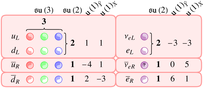
Figure 4: Standard Model (SM). The 15n Weyl fermions of SM contain the representation $(\overline{\bf 3},{\bf 1})_{2,L}\oplus({\bf 1},{\bf 2})_{-3,L}$ $\oplus$ $({\bf 3},{\bf 2})_{1,L}\oplus(\overline{\bf 3},{\bf 1})_{-4,L}\oplus({\bf 1},{\bf 1})_{6,L}$. The 16n Weyl fermions of SM add an extra ${({\bf 1},{\bf 1})_{0,L}}$.

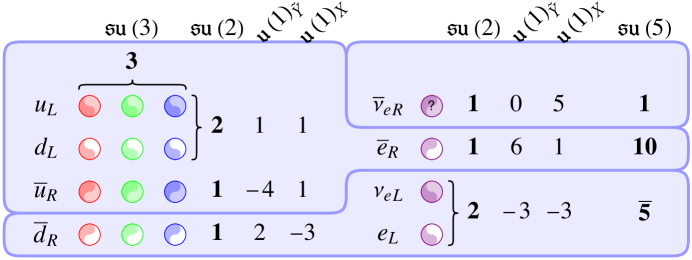
Figure 5: Georgi-Glashow SU(5) model and the $su(5)$ GUT. The 15 Weyl fermions of SM are $\overline{\bf 5}\oplus{\bf 10}$ of SU(5); namely, $(\overline{\bf 3},{\bf 1})_{2,L}\oplus({\bf 1},{\bf 2})_{-3,L}\sim\overline{\bf 5}$ and $({\bf 3},{\bf 2})_{1,L}\oplus(\overline{\bf 3},{\bf 1})_{-4,L}\oplus({\bf 1},{\bf 1})_{6,L}\sim{\bf 10}$ of SU(5). Also $({\bf 1},{\bf 1})_{0,L}\sim{\bf 1}$ of SU(5), so the 16 Weyl fermions of SM are $\overline{\bf 5}\oplus{\bf 10}\oplus{\bf 1}$ of SU(5).

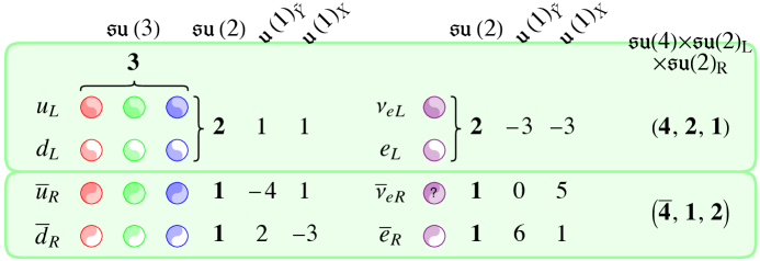
Figure 6: Pati-Salam (PS) model: $G_{\mathrm{PS}_{q^{\prime}}}\equiv\frac{{\rm SU}(4)\times{\rm SU}(2)_{\rm L}\times{\rm SU}(2)_{\rm R}}{\mathbb{Z}_{q^{\prime}}}\equiv\frac{{\rm Spin}(6)\times{\rm Spin}(4)}{\mathbb{Z}_{q^{\prime}}}$ with $q^{\prime}=1,2$. The 16 Weyl fermions of SM are $({\bf 4},{\bf 2},{\bf 1})\oplus(\overline{\bf 4},{\bf 1},{\bf 2})$ of $su(4)\times su(2)_{\mathrm{L}}\times su(2)_{\mathrm{R}}$, and the ${\bf 16}$ of $so(10)$ (or Spin(10)). These L and R are internal symmetry group indices. They are different from (but correlated with) the spacetime symmetry $L$ and $R$. So $({\bf 3},{\bf 2})_{1,L}\oplus({\bf 1},{\bf 2})_{-3,L}\sim({\bf 4},{\bf 2},{\bf 1})_{L}$, and $(\overline{\bf 3},{\bf 1})_{2,L}\oplus(\overline{\bf 3},{\bf 1})_{-4,L}\oplus({\bf 1},{\bf 1})_{6,L}\oplus({\bf 1},{\bf 1})_{0,L}\sim(\overline{\bf 4},{\bf 1},{\bf 2})_{L}$ of PS model.

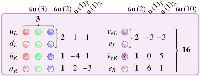
Figure 7: The $so(10)$ GUT model: The 16 Weyl fermions of Spin(10), form the ${\bf 16}$-dimensional representation of Spin(10).

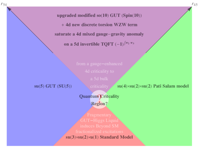
Figure 8: One of our research motif is proposing and investigating this schematic quantum phase diagram. The phase diagram interpolates between different quantum EFT vacua: the $so(10)$ GUT (Spin(10) group), the $su(5)$ GUT (SU(5) group), the $su(4)\times su(2)_{\mathrm{L}}\times su(2)_{\mathrm{R}}$ Pati-Salam model (PS), and the $su(3)\times su(2)\times u(1)$ Standard Model (SM). We will explore the nature of phase transitions later in Sec. 3. We propose the whiten region as a possible quantum critical region, which we explored in Sec. 3 and Sec. 4. Here $r_{\mathbf{R}}$ denotes the coefficient of the effective quadratic potential of $\Phi_{\mathbf{R}}$ field in the representation ${\mathbf{R}}$. The corresponding GUT-Higgs $\Phi_{\mathbf{R}}$ field will condense in the representation-${\mathbf{R}}$ if $r_{\mathbf{R}}<0$. Relatively speaking, the infrared (IR) low energy is drawn with the red color (for SM), the intermediate neighbor phases are drawn with the green or blue color (for PS or SU(5) models), while the ultraviolet (UV) higher energy is drawn with the violet purple color (for Spin(10)); although the readers should keep in mind that we really explore the near-ground-state, zero-energy and zero-temperature quantum phase diagram. These colors are also designed to match the colors of partitions of representations in Fig. 4 to Fig. 7. For Toy Model I without WZW term and without $w_{2}w_{3}$ anomaly, we should remove the whiten quantum critical region, but we are left with a quantum critical point at the origin. For Toy Model II with WZW term and with $w_{2}w_{3}$ anomaly, we encounter the whiten quantum critical region near the origin. The quantum critical region can have dynamical consequences such as emergent deconfined dark gauge force $[{\rm U}(1)^{\prime}]^{\text{emergent}}_{\text{gauge}}$, see Sec. 3.4.2.

In the remaining part of Section 1, we start from an overview on the basic required ingredients of SM and GUT in Sec. 1.1. The outline of this article is given in the table of Contents.

1.1 Various Standard Models and Grand Unifications as Effective Field Theories

Unification, as a central theme in the modern fundamental physics, is a theoretical framework aiming to embody the “elementary” excitations and forces into a common origin. Assuming without any significant dynamical gravity effect at the subatomic scale (i.e., we are only limited to probe the underlying quantum theory by placing the quantum systems on any curved spacetime geometry, but without significant gravity back-reactions), the quantum field theory (QFT) provides a suitable framework for such a unification. Furthermore, assuming that we look at the QFT description valid below a certain energy scale (thus we are ignorant above that energy scale), we shall also implement the effective field theory (EFT) perspective.

In fact, from the EFT perspective, we should remind ourselves the “elementary” excitations are only “elementary” respect to a given EFT quantum vacuum. Moving away from the EFT vacuum (by tuning appropriate physical parameters) to a new quantum vacuum, we shall see that the “elementary” excitations of the new vacuum may be drastically different from the original “elementary” excitations of the previous EFT. So the “elementary” excitations reveal the limitations of our EFT descriptions of quantum vacua. Several examples of such 3+1d QFT and EFT paradigms for high energy physics (HEP) include Standard Model (SM) and Grand Unification (Grand Unified Theory or GUT) [1, 2, 3, 4, 5, 6, 7]:

1. Standard Model (SM) : Glashow-Salam-Weinberg (GSW) [1, 2, 3, 4] proposed the electroweak theory of the unified electromagnetic and weak forces between elementary particles. The GSW theory together with the strong force [32, 33] becomes the Standard Model (SM), which is essential to describe the subatomic particle physics. The SM gauge group can be

   $$G_{{\rm SM}_{q}}\equiv\frac{{{\rm SU}(3)}_{c}\times{{\rm SU}(2)}_{\rm L}\times{\rm U}(1)_{\tilde{Y}}}{\mathbb{Z}_{q}}$$

   with the mod $q=1,2,3,6$ so far undetermined by the current experiments (see an overview [34, 35] on this global structure of SM Lie group issue). The subscript $c$ is for color, the L is for the internal SU(2) (L for internal symmetry and its spinor) locked with the left-handed Weyl fermion ($L$ for spacetime symmetry and its spinor) in the standard HEP convention, and ${\tilde{Y}}$ for electroweak hypercharge. The “elementary” particle excitations of this SM EFT, with 15n or 16n Weyl fermions, are constrained by the representation of $su(3)\times su(2)\times u(1)$ as (see Fig. 4):

   $${(\overline{\bf 3},{\bf 1})_{2,L}\oplus({\bf 1},{\bf 2})_{-3,L}\oplus({\bf 3},{\bf 2})_{1,L}\oplus(\overline{\bf 3},{\bf 1})_{-4,L}\oplus({\bf 1},{\bf 1})_{6,L}\oplus{({\bf 1},{\bf 1})_{0,L}}}.$$ (1.3)

   The 16th Weyl fermion ${({\bf 1},{\bf 1})_{0,L}}$ is an extra sterile neutrino, sterile to the SM gauge force, also called the right-handed neutrino. We will focus on the 16n Weyl fermion model in this present work. In our convention, we write Weyl fermions in the left-handed ($L$) basis which means that each is a 2-component ${\bf 2}_{L}$ spinor of the spacetime symmetry group Spin(1,3).

2. The $su(5)$ Grand Unification ($su(5)$ GUT): Georgi-Glashow (GG) [5] hypothesized that at a higher energy, the three SM gauge interactions merged into a single electronuclear force under a simple Lie algebra $su(5)$, or precisely a Lie group

   $$G_{\mathrm{GG}}\equiv{\rm SU}(5)$$

   gauge theory. The su(5) GUT works for 15n Weyl fermions, also for 16n Weyl fermions (i.e., 15 or 16 Weyl fermions per generation). The “elementary” particle excitations of this SU(5) EFT, with 15n or 16n Weyl fermions, are constrained by the representation of SU(5) as (see Fig. 5):

   $$\overline{\bf 5}\oplus{\bf 10}\oplus{\bf 1},$$ (1.4)

   again written all in the left-handed ($L$) Weyl basis. The 16th Weyl fermion is an extra sterile neutrino, sterile to the SU(5) gauge force, also called the right-handed neutrino.

3. The Pati-Salam model (PS model): Pati-Salam (PS) [6] hypothesized that the lepton forms the fourth color, extending SU(3) to SU(4). The PS also puts the left ${\rm SU}(2)_{\mathrm{L}}$ and a hypothetical right ${\rm SU}(2)_{\mathrm{R}}$ on equal footing. The PS gauge Lie algebra is $su(4)\times su(2)_{\mathrm{L}}\times su(2)_{\mathrm{R}}$, and the PS gauge Lie group is

   $$G_{\mathrm{PS}_{q^{\prime}}}\equiv\frac{{\rm SU}(4)_{c}\times({\rm SU}(2)_{\mathrm{L}}\times{\rm SU}(2)_{\mathrm{R}})}{\mathbb{Z}_{q^{\prime}}}=\frac{{\rm Spin}(6)\times{\rm Spin}(4)}{\mathbb{Z}_{q^{\prime}}}$$

   with the mod $q^{\prime}=1,2$ depending on the global structure of Lie group. The “elementary” particle excitations of this PS EFT, with 16n Weyl fermions, are constrained by the representation of $G_{\mathrm{PS}_{q^{\prime}}}$as (see Fig. 6):

   $$({\bf 4},{\bf 2},{\bf 1})\oplus(\overline{\bf 4},{\bf 1},{\bf 2}),$$ (1.5)

   written all in the left-handed ($L$) Weyl basis.

4. The $so(10)$ Grand Unification ($so(10)$ GUT): Georgi and Fritzsch-Minkowski [7] hypothesized that quarks and leptons become the 16-dimensional spinor representation

   $${\bf 16}^{+} G_{so(10)}\equiv{\rm Spin}(10)$$ of gauge group (1.6)

   (with a local Lie algebra $so(10)$). Thus, the 16n Weyl fermions can interact via the Spin(10) gauge fields at a higher energy. In this case, the 16th Weyl fermion, previously a sterile neutrino to the SU(5), is no longer sterile to the Spin(10) gauge fields; it also carries a charge 1, thus not sterile, under the gauged center subgroup $Z({\rm Spin}(10))=\mathbb{Z}_{4}$.

We relegate several tables of data relevant for SMs and GUTs into Appendix A, for readers’ convenience to check the quantum numbers of various elementary particles or field quanta of SMs and GUTs.

2 Standard Models from the competing phases of Grand Unifications

In Sec. 2, we start by enlisting and explaining some group embedding structures from some of relevant GUTs to SM in Sec. 2.1.

2.1 Spacetime-Internal Symmetry Group embedding of SMs and GUTs, and the $w_{2}w_{3}$ anomaly

Here we use the inclusion notation $G_{\text{large}}\hookleftarrow G_{\text{small}}$ to imply that:

• $G_{\text{large}}\supset G_{\text{small}}$, namely the $G_{\text{large}}$ contains $G_{\text{small}}$ as a subgroup, or equivalently $G_{\text{small}}$ can be embedded in $G_{\text{large}}$.

• $G_{\text{large}}$ can be broken to $G_{\text{small}}$ via symmetry breaking of Higgs condensation (which we will explore).

The internal symmetry group embedding structure has been explored, for example summarized in [39]:

(2.5)

We further include both the complete spacetime-internal symmetry group embedding structure as follows:

$$\bar{G}\equiv{{G_{\text{spacetime}}}\times_{{N_{\text{shared}}}}{{G}_{\text{internal}}}}\equiv({\frac{{G_{\text{spacetime}}}\times{{G}_{\text{internal}}}}{{N_{\text{shared}}}}}).$$ (2.6)

$$\lx@xy@svg{\hbox{\raise 0.0pt\hbox{\kern 76.44118pt\hbox{\ignorespaces\ignorespaces\ignorespaces\hbox{\vtop{\kern 0.0pt\offinterlineskip\halign{\entry@#!@&&\entry@@#!@\cr&\\&\\}}}\ignorespaces{\hbox{\kern-76.44118pt\raise 0.0pt\hbox{\hbox{\kern 0.0pt\raise 0.0pt\hbox{\hbox{\kern 3.0pt\raise 0.0pt\hbox{$\textstyle{{\bar{G}_{{\rm SM}_{6}}\equiv{\rm Spin}\times_{\mathbb{Z}_{2}^{F}}\mathbb{Z}_{4,X}\times\frac{{{\rm SU}(3)}_{c}\times{{\rm SU}(2)}_{\rm L}\times{\rm U}(1)_{Y}}{\mathbb{Z}_{6}}}\ignorespaces\ignorespaces\ignorespaces\ignorespaces\ignorespaces\ignorespaces\ignorespaces\ignorespaces}$}}}}}}}\ignorespaces\ignorespaces\ignorespaces\ignorespaces{\hbox{\kern 76.4412pt\raise 0.0pt\hbox{\hbox{\kern 0.0pt\raise 0.0pt\hbox{\lx@xy@hook{1}}}}}}{\hbox{\lx@xy@droprule}}\ignorespaces{\hbox{\kern 100.44118pt\raise 0.0pt\hbox{\hbox{\kern 0.0pt\raise 0.0pt\hbox{\lx@xy@tip{1}\lx@xy@tip{-1}}}}}}{\hbox{\lx@xy@droprule}}{\hbox{\lx@xy@droprule}}\ignorespaces\ignorespaces\ignorespaces\ignorespaces{\hbox{\kern 0.0pt\raise-6.4911pt\hbox{\hbox{\kern 0.0pt\raise 0.0pt\hbox{\lx@xy@hook{1}}}}}}{\hbox{\lx@xy@droprule}}\ignorespaces{\hbox{\kern 0.0pt\raise-28.7636pt\hbox{\hbox{\kern 0.0pt\raise 0.0pt\hbox{\lx@xy@tip{1}\lx@xy@tip{-1}}}}}}{\hbox{\lx@xy@droprule}}{\hbox{\lx@xy@droprule}}{\hbox{\kern 100.44118pt\raise 0.0pt\hbox{\hbox{\kern 0.0pt\raise 0.0pt\hbox{\hbox{\kern 3.0pt\raise 0.0pt\hbox{$\textstyle{\bar{G}_{\mathrm{GG}}\equiv{\rm Spin}\times_{\mathbb{Z}_{2}^{F}}\mathbb{Z}_{4,X}\times{\rm SU}(5)\ignorespaces\ignorespaces\ignorespaces\ignorespaces}$}}}}}}}\ignorespaces\ignorespaces\ignorespaces\ignorespaces{\hbox{\kern 158.5362pt\raise-6.4911pt\hbox{\hbox{\kern 0.0pt\raise 0.0pt\hbox{\lx@xy@hook{1}}}}}}{\hbox{\lx@xy@droprule}}\ignorespaces{\hbox{\kern 158.5362pt\raise-35.58247pt\hbox{\hbox{\kern 0.0pt\raise 0.0pt\hbox{\lx@xy@tip{1}\lx@xy@tip{-1}}}}}}{\hbox{\lx@xy@droprule}}{\hbox{\lx@xy@droprule}}{\hbox{\kern-65.88351pt\raise-46.08247pt\hbox{\hbox{\kern 0.0pt\raise 0.0pt\hbox{\hbox{\kern 3.0pt\raise 0.0pt\hbox{$\textstyle{\displaystyle{\bar{G}_{\mathrm{PS}_{2}}\equiv{\rm Spin}\times_{\mathbb{Z}_{2}^{F}}\frac{{\rm Spin}(6)\times{\rm Spin}(4)}{\mathbb{Z}_{2}}}\ignorespaces\ignorespaces\ignorespaces\ignorespaces}$}}}}}}}\ignorespaces\ignorespaces\ignorespaces\ignorespaces{\hbox{\kern 65.88353pt\raise-46.08247pt\hbox{\hbox{\kern 0.0pt\raise 0.0pt\hbox{\lx@xy@hook{1}}}}}}{\hbox{\lx@xy@droprule}}\ignorespaces{\hbox{\kern 104.2664pt\raise-46.08247pt\hbox{\hbox{\kern 0.0pt\raise 0.0pt\hbox{\lx@xy@tip{1}\lx@xy@tip{-1}}}}}}{\hbox{\lx@xy@droprule}}{\hbox{\lx@xy@droprule}}{\hbox{\kern 104.2664pt\raise-46.08247pt\hbox{\hbox{\kern 0.0pt\raise 0.0pt\hbox{\hbox{\kern 3.0pt\raise 0.0pt\hbox{$\textstyle{\bar{G}_{so(10)}\equiv{\rm Spin}\times_{\mathbb{Z}_{2}^{F}}{\rm Spin}(10)}$}}}}}}}\ignorespaces}}}}\ignorespaces. \textstyle{{\bar{G}_{{\rm SM}_{6}}\equiv{\rm Spin}\times_{\mathbb{Z}_{2}^{F}}\mathbb{Z}_{4,X}\times\frac{{{\rm SU}(3)}_{c}\times{{\rm SU}(2)}_{\rm L}\times{\rm U}(1)_{Y}}{\mathbb{Z}_{6}}}\ignorespaces\ignorespaces\ignorespaces\ignorespaces\ignorespaces\ignorespaces\ignorespaces\ignorespaces} \textstyle{\bar{G}_{\mathrm{GG}}\equiv{\rm Spin}\times_{\mathbb{Z}_{2}^{F}}\mathbb{Z}_{4,X}\times{\rm SU}(5)\ignorespaces\ignorespaces\ignorespaces\ignorespaces} \textstyle{\displaystyle{\bar{G}_{\mathrm{PS}_{2}}\equiv{\rm Spin}\times_{\mathbb{Z}_{2}^{F}}\frac{{\rm Spin}(6)\times{\rm Spin}(4)}{\mathbb{Z}_{2}}}\ignorespaces\ignorespaces\ignorespaces\ignorespaces} \textstyle{\bar{G}_{so(10)}\equiv{\rm Spin}\times_{\mathbb{Z}_{2}^{F}}{\rm Spin}(10)} \textstyle{{\bar{G}_{{\rm SM}_{6}}\equiv{\rm Spin}\times_{\mathbb{Z}_{2}^{F}}\mathbb{Z}_{4,X}\times\frac{{{\rm SU}(3)}_{c}\times{{\rm SU}(2)}_{\rm L}\times{\rm U}(1)_{Y}}{\mathbb{Z}_{6}}}\ignorespaces\ignorespaces\ignorespaces\ignorespaces\ignorespaces\ignorespaces\ignorespaces\ignorespaces} \textstyle{\bar{G}_{\mathrm{GG}}\equiv{\rm Spin}\times_{\mathbb{Z}_{2}^{F}}\mathbb{Z}_{4,X}\times{\rm SU}(5)\ignorespaces\ignorespaces\ignorespaces\ignorespaces} \textstyle{\displaystyle{\bar{G}_{\mathrm{PS}_{2}}\equiv{\rm Spin}\times_{\mathbb{Z}_{2}^{F}}\frac{{\rm Spin}(6)\times{\rm Spin}(4)}{\mathbb{Z}_{2}}}\ignorespaces\ignorespaces\ignorespaces\ignorespaces} \textstyle{\bar{G}_{so(10)}\equiv{\rm Spin}\times_{\mathbb{Z}_{2}^{F}}{\rm Spin}(10)}$$ (2.11)

Some comments about (2.11) follow:

1. The ${\rm Spin}$ means the spacetime rotational symmetry group ${\rm Spin}\equiv{\rm Spin}(1,3)$ for 4d Lorentz signature (or ${\rm Spin}\equiv{\rm Spin}(4)$ for 4d Euclidean signature). The ${\rm Spin}$ contains the fermionic parity $\mathbb{Z}_{2}^{F}$ at the center subgroup thus ${{\rm Spin}}/{\mathbb{Z}_{2}^{F}}={\rm SO}$ where the ${\rm SO}$ is the bosonic spacetime (special orthogonal) rotational symmetry group (similarly, ${\rm SO}\equiv{\rm SO}(1,3)$ for 4d Lorentz signature, or ${\rm SO}\equiv{\rm SO}(4)$ for 4d Euclidean signature). The notation $G_{1}\times_{N_{\text{shared}}}G_{2}\equiv\frac{G_{1}\times G_{2}}{{N_{\text{shared}}}}$ means modding out their common normal subgroup ${N_{\text{shared}}}$. So ${\rm Spin}\times_{\mathbb{Z}_{2}^{F}}G\equiv\frac{{\rm Spin}\times G}{{\mathbb{Z}_{2}^{F}}}$ means modding out their common normal subgroup ${\mathbb{Z}_{2}^{F}}$.

2. The $\mathbb{Z}_{4,X}$ has the $X$-symmetry generator such that its square $(X)^{2}=(-1)^{F}$ is the fermion parity operator, so $\mathbb{Z}_{4,X}\supset\mathbb{Z}_{2}^{F}$. Wilczek-Zee [40] firstly noticed that the $X\equiv 5({\mathbf{B}-\mathbf{L}})-4Y$, with the baryon minus lepton number ${\mathbf{B}-\mathbf{L}}$ and the electroweak hypercharge $Y$, is a good global symmetry respected by SM and the $su(5)$ GUT. All known quarks and leptons carry a charge 1 of $\mathbb{Z}_{4,X}$, in the left-handed Weyl spinor basis. The center of Spin(10) can be chosen exactly as $Z({\rm Spin}(10))=\mathbb{Z}_{4,X}$. We summarize how $\mathbb{Z}_{4,X}$ can be obtained in Table 3 and Table 4. See more discussions on $\mathbb{Z}_{4,X}$ in [21, 24, 36, 37, 38].

3. The $(X)^{2}=(-1)^{F}$ relation is obeyed in the non-supersymmetric SM and GUT models, so it is natural to introduce the ${\rm Spin}\times_{\mathbb{Z}_{2}^{F}}\mathbb{Z}_{4,X}$ structure in (2.11). However, it is possible to have new fermions, such as in supersymmetric SMs or GUTs, which does not necessarily obey $(X)^{2}=(-1)^{F}$ relation. In that case, we can introduce just ${\rm Spin}\times\mathbb{Z}_{4,X}$ structure. See a footnote for the alternative symmetry embedding with the ${\rm Spin}\times\mathbb{Z}_{4,X}$ structure.

4. In this (2.11), we keep a structure of ${\rm Spin}\times_{\mathbb{Z}_{2}^{F}}\mathbb{Z}_{4,X}$ which is essential to produce a mixed gauge-gravity nonperturbative global anomaly constraint of a $\mathbb{Z}_{16}$ class. As already mentioned in footnote 12, in this article, we keep the 16n Weyl fermions in all our SM and GUT models, thus the $\mathbb{Z}_{16}$ global anomaly is already cancelled by 16n chiral fermions.

5. In this (2.11), we also keep a structure of ${\rm Spin}\times_{\mathbb{Z}_{2}^{F}}{\rm Spin}(10)$ — the cobordism group $\Omega^{d}_{G}\equiv\mathrm{TP}_{d}(G)$ shows [12, 22]

   $$\mathrm{TP}_{5}({\rm Spin}\times_{\mathbb{Z}_{2}^{F}}{\rm Spin}(10))=\mathbb{Z}_{2} \mathrm{TP}_{5}({\rm Spin}\times{\rm Spin}(10))=0$$,  but . (2.17)

   This implies only the ${\rm Spin}\times_{\mathbb{Z}_{2}^{F}}{\rm Spin}(10)$ structure offers a possible $\mathbb{Z}_{2}$ class global anomaly in 4d that is captured by a 5d invertible TQFT with a partition function on a 5d manifold $M^{5}$:

   $${\bf Z}(M^{5})=(-1)^{\int_{M^{5}}w_{2}(TM)w_{3}(TM)}=(-1)^{\int_{M^{5}}w_{2}(V_{{\rm SO}(10)})w_{3}(V_{{\rm SO}(10)})}.$$ (2.20)

   But this mod 2 anomaly is absent and not allowed on the ${\rm Spin}\times{\rm Spin}(10)$ structure. The difference between ${\rm Spin}\times_{\mathbb{Z}_{2}^{F}}{\rm Spin}(10)$ and ${\rm Spin}\times{\rm Spin}(10)$ is the following: the fermion charge under $(-1)^{F}$ thus odd under ${\mathbb{Z}_{2}^{F}}$ must be in the $\mathbb{Z}_{2}$ normal subgroup of the center subgroup $Z({\rm Spin}(10))=\mathbb{Z}_{4,X}$ so $(X)^{2}=(-1)^{F}$ in order to impose the spacetime-internal ${\rm Spin}\times_{\mathbb{Z}_{2}^{F}}{\rm Spin}(10)$ structure. However, in contrast, the ${\rm Spin}\times{\rm Spin}(10)$ allows other fermions to not obey the $(X)^{2}=(-1)^{F}$ relation.

   As mentioned in Ref. [12, 17] and footnote 7, as ${\rm Spin}(10)\supset{\rm Spin}(3)={\rm SU}(2)$, so

   $${\rm Spin}\times_{\mathbb{Z}_{2}^{F}}{\rm Spin}(10)\supset{\rm Spin}\times_{\mathbb{Z}_{2}^{F}}{\rm Spin}(3)={\rm Spin}\times_{\mathbb{Z}_{2}^{F}}{\rm SU}(2).$$ (2.21)

   The ${\rm Spin}\times_{\mathbb{Z}_{2}^{F}}{\rm Spin}(10)$-structure is tightly related to the ${\rm Spin}\times_{\mathbb{Z}_{2}^{F}}{\rm SU}(2)$ also known as the ${\rm Spin}^{h}$-structure. We can project the ${\rm Spin}\times_{\mathbb{Z}_{2}^{F}}{\rm Spin}(10)$-structure to the ${\rm Spin}^{h}$-structure. Then, in the ${\rm Spin}^{h}$-structure, because the fermionic wavefunction gains a $(-1)$ statistical sign under a $2\pi$ self rotation on a Spin manifold is identified with the $(-1)^{F}$ as the center $Z({\rm SU}(2))=\mathbb{Z}_{2}^{F}$, we can read that imposing the ${\rm Spin}^{h}$-structure [12, 17]:
   $\bullet$ the fermions must be in the half-integer isospin representation 1/2, 3/2, $\dots$, etc. of SU(2) (namely, the even-dimensional representations ${\bf 2},{\bf 4},\dots,$ etc. of SU(2)).
   $\bullet$ the bosons must be in the integer isospin representation 0, 1, 2, $\dots$, etc. of SU(2) (namely, the odd-dimensional representations ${\bf 0},{\bf 1},{\bf 3},\dots,$ etc. of SU(2)).

6. The last but the most important comment above all, is that in order to realize a possible continuous deconfined quantum phase transition, we do require to use the $w_{2}w_{3}$ anomaly in (2.20), such that this anomaly occurs in the phase transition between the GG and PS models in Fig. 8. So we do aim to impose the ${\rm Spin}\times_{\mathbb{Z}_{2}^{F}}{\rm Spin}(10)$-structure as in (2.11) in order to implement the $w_{2}w_{3}$ anomaly. In short, the readers can ask:

   $$\text{\emph{Why do we need the $w_{2}w_{3}$ anomaly near the criticality for establishing}}\cr\text{\emph{a possible continuous quantum phase transition between the GG and PS models?}}$$ (2.22)

   The answer is that:
   $\bullet$ The GG and PS models are Landau-Ginzburg symmetry breaking type of phases (when we treat the internal symmetry as global symmetry) or the gauge-symmetry breaking type of phases (when we treat the internal symmetry group as gauge group). The $w_{2}w_{3}$ anomaly is matched on two sides of phases by GG and PS models via symmetry breaking. (In fact, no $w_{2}w_{3}$ anomaly is allowed in GG and PS models.)
   $\bullet$ But the $w_{2}w_{3}$ anomaly can protect a gapless quantum phase transition (or a gapless intermediate quantum critical region) between the GG and PS models when the Spin(10) symmetry is restored at their phase transition. Their phase transition can be protected to be Spin(10)-symmetry-preserving gapless due to the $w_{2}w_{3}$ anomaly exists only in the enlarged Spin(10) internal symmetry group.

   Because the conventional $so(10)$ GUT is free from the $w_{2}w_{3}$ anomaly [12, 17], we will need to explicitly introduce a new WZW-like term built out of GUT-Higgs field in the mother EFT, which allows the GUT-Higgs sector (beyond the SM sector) to saturate the $w_{2}w_{3}$ anomaly. To this end, we will start from writing down a GUT-Higgs model in the context of $so(10)$ GUT, and then trying to modifying the GUT-Higgs model to saturate the $w_{2}w_{3}$ anomaly. (That mother EFT will be the main achievement later in Sec. 3.)

2.2 Branching Rule of SMs and GUTs, and a GUT-Higgs model

In the following, we motivate the GUT model with GUT-Higgs as the gauge symmetry breaking pattern to go to the lower energy EFT (such as SM). Most of these breaking patterns are well-established and overviewed in [41]. The additional new input is that we try to unify several models into a GUT-Higgs model with as minimum amount of GUT-Higgs as possible. In Appendix B, we try to go through the logic again, and carefully examine the consequences and possibilities of the types of required GUT-Higgs. Later we will motivate the possible Lagrangian of the GUT-Higgs potential.

Here we summarize what we need from the analysis done in Appendix B:

• We can use a Lorentz scalar boson with a 45-dimensional real representation of $so(10)$ or Spin(10):

  $$\Phi_{so(10),\bf 45}\equiv\Phi_{\bf 45}\in{\mathbb{R}}.$$ (2.23)

  to break the ${\rm Spin}(10)$ of $so(10)$ GUT to the ${\rm SU}(5)$ of GG model, also we can use this same $\Phi_{\bf 45}$ to break $G_{\mathrm{PS}_{2}}\equiv\frac{{\rm Spin}(6)\times{\rm Spin}(4)}{\mathbb{Z}_{2}}$ of PS model to the $G_{{\rm SM}_{6}}\equiv\frac{{{\rm SU}(3)}_{c}\times{{\rm SU}(2)}_{\rm L}\times{\rm U}(1)_{Y}}{\mathbb{Z}_{6}}$ of the SM.

• We can use a Lorentz scalar boson with a 54-dimensional real representation of $so(10)$ or Spin(10):

  $$\Phi_{so(10),\bf 54}\equiv\Phi_{\bf 54}\in{\mathbb{R}},$$ (2.24)

  to break the ${\rm Spin}(10)$ of $so(10)$ GUT to the $G_{\mathrm{PS}_{2}}\equiv\frac{{\rm Spin}(6)\times{\rm Spin}(4)}{\mathbb{Z}_{2}}$ of PS model, also we can use this same $\Phi_{\bf 54}$ to break ${\rm SU}(5)$ of GG model to the $G_{{\rm SM}_{6}}\equiv\frac{{{\rm SU}(3)}_{c}\times{{\rm SU}(2)}_{\rm L}\times{\rm U}(1)_{Y}}{\mathbb{Z}_{6}}$ of the SM.

• The combinations of the two facts above is summarized in Fig. 9, where we can use the $\Phi_{\bf 45}$ and $\Phi_{\bf 54}$ to write the GUT-Higgs model, that can induce the qualitative phase diagram similar to Fig. 8.

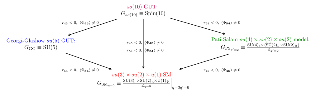
Figure 9: Beware that the direction of the group symmetry breaking “$\rightarrow$” is the opposite direction to the group inclusion “$\hookleftarrow$.” (These colors are also designed to match the colors in Fig. 4 to Fig. 7, and Fig. 8).

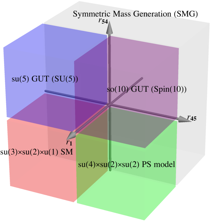
Figure 10: Schematic quantum phase diagram interpolating between the $so(10)$ GUT (Spin(10) group), the Georgi-Glashow $su(5)$ GUT (SU(5) group), the $su(4)\times su(2)_{\mathrm{L}}\times su(2)_{\mathrm{R}}$ Pati-Salam model (PS), and the $su(3)\times su(2)\times u(1)$ Standard Model (SM), and the symmetric mass generation (SMG). Here the real parameter $r_{\mathbf{R}}\in{\mathbb{R}}$ denotes the coefficient of the effective quadratic potential of $\Phi$ field in the representation ${\mathbf{R}}$. The corresponding GUT-Higgs $\Phi$ field will condense in the representation-${\mathbf{R}}$ if $r_{\mathbf{R}}<0$. Relatively speaking, the infrared (IR) low energy is drawn with the red color (for SM), the intermediate neighbor phases are drawn with the green or blue color (for PS or SU(5) models), while the ultraviolet (UV) higher energy is drawn with the violet purple color (for Spin(10)). These colors are also designed to match the colors of partitions of representations in Fig. 4 to Fig. 7.

Given the $so(10)$ GUT, to induce the three other models in Fig. 9, we can add the GUT-Higgs potential ${\rm U}(\Phi_{{\mathbf{R}}})$ with $\Phi_{{\mathbf{R}}}$ of some representation ${\mathbf{R}}$. The ${\rm U}(\Phi_{{\mathbf{R}}})$ is chosen to have positive $\Phi^{4}$ coefficients (thus $\lambda_{{\mathbf{45}}},\lambda_{{\mathbf{54}}}>0$), while the $r_{{\mathbf{45}}}$ and $r_{{\mathbf{54}}}$ are real-number tunable parameters shown in Fig. 8 and Fig. 10:

$${\rm U}(\Phi_{{\mathbf{R}}})=\Big{(}r_{{\mathbf{45}}}(\Phi_{{\mathbf{45}}})^{2}+\lambda_{{\mathbf{45}}}(\Phi_{{\mathbf{45}}})^{4}\Big{)}+\Big{(}r_{{\mathbf{54}}}(\Phi_{{\mathbf{54}}})^{2}+\lambda_{{\mathbf{54}}}(\Phi_{{\mathbf{54}}})^{4}\Big{)}.$$ (2.25)

A slice of Fig. 10 becomes the Fig. 8. (Temporarily now we get rid of the GUT-Higgs $\Phi_{\mathbf{1}}$ thus get rid of $r_{{\mathbf{1}}}$ axis in Fig. 10. More on this $\Phi_{\mathbf{1}}$ later.) We can use this ${\rm U}(\Phi_{{\mathbf{R}}})$ potential in (2.25) to induce these interior parts of four phases (the $so(10)$ GUT, the $su(5)$ GUT, the PS model, and the SM).

• If $\langle\Phi_{\mathbf{45}}\rangle$ condenses, namely if $r_{{\mathbf{45}}}<0$ so $\langle\Phi_{\mathbf{45}}\rangle\neq 0$, then the $so(10)$ GUT becomes Higgs down to the $su(5)$ GUT.

• If $\langle\Phi_{\mathbf{54}}\rangle$ condenses, namely if $r_{{\mathbf{54}}}<0$ so $\langle\Phi_{\mathbf{54}}\rangle\neq 0$, then the $so(10)$ GUT becomes Higgs down to the PS model.

• If $\langle\Phi_{\mathbf{45}}\rangle$ and $\langle\Phi_{\mathbf{54}}\rangle$ both condense, namely if $r_{{\mathbf{45}}}<0$ and $r_{{\mathbf{54}}}<0$ so that $\langle\Phi_{\mathbf{45}}\rangle\neq 0$ and $\langle\Phi_{\mathbf{54}}\rangle\neq 0$. The theory becomes Higgs down to the SM.

All these above Higgs condensations induce continuous phase transitions.

The purpose of the next Section 3 is to design various EFT and to explore the possible phase structures and phase transitions (of Fig. 8 and Fig. 10). In particular, we will write down a mother EFT such that it saturates the $w_{2}w_{3}$ global anomaly and it realizes an excotic quantum phase transition between the GG $su(5)$ GUT and the PS model.

3 Mother Effective Field Theory with Competing GUT-Higgs fields

3.1 Elementary GUT-Higgs model induces the SM

In Section 2 (especially Sec. 2.2), we write down a GUT-Higgs potential ${\rm U}(\Phi_{{\mathbf{R}}})$ in (2.25) appending to the $so(10)$ GUT with 16n complex Weyl fermions $\psi_{L}$. Let us write down the full path integral ${\mathbf{Z}}_{{\rm GUT}}$ of such $so(10)$ GUT plus ${\rm U}(\Phi_{{\mathbf{R}}})$, in a Lorentzian signature, evaluated on a 4-manifold $M^{4}$:

$${\mathbf{Z}}_{{\rm GUT}}\equiv\int[{\cal D}{\psi_{L}}][{\cal D}{\psi_{L}^{\dagger}}][{\cal D}A][{\cal D}\Phi_{{\mathbf{R}}}]\dots\exp(\hskip 1.0pt\mathrm{i}\hskip 1.0pt\left.S_{\text{GUT}}[\psi_{L},{\psi_{L}^{\dagger}},A,\Phi_{{\mathbf{R}}},\dots]\right\rvert_{M^{4}}).$$ (3.1)

The action $S_{\text{GUT}}$ is:

$$S_{\text{GUT}}=\int_{M^{4}}\Big{(}{\mathrm{Tr}}(F\wedge\star F)-\frac{\theta}{8\pi^{2}}g^{2}{\mathrm{Tr}}(F\wedge F)\Big{)}+\int_{M^{4}}\Big{(}{\psi}^{\dagger}_{L}(\hskip 1.0pt\mathrm{i}\hskip 1.0pt{\bar{\sigma}}^{\mu}{D}_{\mu,A})\psi_{L}\\ +|{D}_{\mu,A}\Phi_{{\mathbf{R}}}|^{2}-{\rm U}(\Phi_{{\mathbf{R}}})-((\Phi_{{\mathbf{R}}})({\psi}^{\dagger}_{L}\cdots)({\psi}_{L}\cdots)+{\rm h.c.})+\dots\Big{)}\,\hskip 1.0pt\mathrm{d}^{4}x.$$ (3.2)

The $S_{\text{YM}}=\int{\mathrm{Tr}}(F\wedge\star F)$ part is the Yang-Mills gauge theory, with Lie algebra valued field strength curvature 2-form $F=\hskip 1.0pt\mathrm{d}A-\hskip 1.0pt\mathrm{i}\hskip 1.0pt{g}A\wedge A$. Here $({\psi}^{\dagger}_{L}\cdots)$ and $({\psi}_{L}\cdots)$ imply indefinite multiple numbers of Weyl fermion fields, so as to properly match the representation $\mathbf{R}$ of the Higgs field $\Phi_{\mathbf{R}}$. For the $so(10)$ GUT, we have to sum over the Spin(10) gauge bundle, whose 1-form connection is the spin-1 Lorentz vector and Spin(10) gauge field, written as

$$A=(\sum_{\mathrm{a}=1}^{45}{{\rm T}^{\mathrm{a}}}A_{{{\rm Spin}(10)},\mu}^{\mathrm{a}})\hskip 1.0pt\mathrm{d}x^{\mu}.$$ (3.3)

There are 45 of such Lie algebra generators, ${{\rm T}^{\mathrm{a}}}$, with:
$\bullet$ rank-16 matrix representations that act on the quark-and-lepton matter representation ${\bf 16}^{+}$ of Spin(10).
$\bullet$ rank-45 matrix representations that act on the $\Phi_{\mathbf{45}}$ as the ${\bf 45}$ of Spin(10).
$\bullet$ rank-54 matrix representations that act on the $\Phi_{\mathbf{54}}$ as the ${\bf 54}$ of Spin(10).

Locally the Spin(10) Lie algebra is the same as the $so(10)$ Lie algebra, but globally we really need to define the principal Spin(10) gauge bundle $P_{A}$ to sum over. So more precisely the path integral over the gauge field measure really means $\int[{\cal D}A]\dots\equiv\sum_{\text{gauge bundle $P_{A}$}}\int[{\cal D}\tilde{A}]\dots$, where $\tilde{A}$ are gauge connections over each specific gauge bundle choice $P_{A}$. The $\theta$ term, $\theta{\mathrm{Tr}}(F\wedge F)$, can be added or removed depending on the model. In this work, we shall set $\theta=0$ or close to zero.

The $\psi_{L}$ is a 2-component spin-1/2 Weyl fermion ${\bf 2}_{L}$ of Spin(1,3). The $\dagger$ is the standard complex conjugate transpose. The $\bar{\sigma}^{\mu}=(\sigma^{0},-\sigma^{1},-\sigma^{2},-\sigma^{3})$ and ${\sigma}^{\mu}=(\sigma^{0},\sigma^{1},\sigma^{2},\sigma^{3})$ are the standard spacetime spinor rotational $su(2)$ Lie algebra generators for $L$ and $R$ Weyl spinors. The action $S_{\text{GUT}}$ also includes the Weyl spinor kinetic term and GUT-Higgs kinetic term, coupling to gauge fields via the covariant derivative operator ${D}_{\mu,A}\equiv\nabla_{\mu}-\hskip 1.0pt\mathrm{i}\hskip 1.0ptg\,A_{\mu}$. The $\nabla_{\mu}$ can contain the curve-spacetime covariant derivative data such as Christoffel symbols or the spinor’s spin-connection if needed. The $\dots$ are possible extra deformation terms to be added later.

This subsection Sec. 3.1 mostly treats the spin-0 Lorentz scalar Higgs field $\Phi_{\bf R}$ with some representation ${\bf R}$ as the elementary Higgs field. We will however fractionalize this elementary Higgs field $\Phi_{\bf R}$ to other further elementary fermionic fields in the later Sec. 3.3 and Sec. 3.4.

3.1.1 Model I: Without Wess-Zumino-Witten term, and Symmetric Mass Generation

Follow the choice in Sec. 2.2 and in (2.25), we can further adjust it to

$${\rm U}(\Phi_{{\mathbf{R}}})=\Big{(}r_{{\mathbf{45}}}(\Phi_{{\mathbf{45}}})^{2}+\lambda_{{\mathbf{45}}}(\Phi_{{\mathbf{45}}})^{4}\Big{)}+\Big{(}r_{{\mathbf{54}}}(\Phi_{{\mathbf{54}}})^{2}+\lambda_{{\mathbf{54}}}(\Phi_{{\mathbf{54}}})^{4}\Big{)}+\Big{(}r_{{\mathbf{1}}}(\Phi_{{\mathbf{1}}})^{2}+\lambda_{{\mathbf{1}}}(\Phi_{{\mathbf{1}}})^{4}\Big{)}.$$ (3.4)

The property (whether $\langle\Phi_{\mathbf{45}}\rangle\neq 0$ or $\langle\Phi_{\mathbf{54}}\rangle\neq 0$ condenses, or both condense, namely whether $r_{{\mathbf{54}}}<0$ or $r_{{\mathbf{54}}}<0$) still follows Sec. 2.2. The theory becomes Higgs down to the $su(5)$ GUT, or the PS model, or the SM, see Fig. 9. Here are some extra comments for adding $\Phi_{\mathbf{1}}$ or other $\Phi_{\mathbf{R}}$ terms to Fig. 10:

• We can introduce a Lorentz scalar boson with a 1-dimensional trivial but real representation of $so(10)$ or Spin(10):

  $$\Phi_{so(10),\bf 1}\equiv\Phi_{\bf 1}\in{\mathbb{R}}.$$ (3.5)

  • If $\langle\Phi_{\mathbf{1}}\rangle=0$ does not condense, namely if $r_{{\mathbf{1}}}>0$, the theory remains in the $so(10)$ GUT.

  • If $\langle\Phi_{\mathbf{1}}\rangle\neq 0$ condenses, namely if $r_{{\mathbf{1}}}<0$, for a small $\langle\Phi_{\mathbf{1}}\rangle<\Phi_{{\mathbf{1}},c}$, the theory still remains in the $so(10)$ GUT (as $\langle\Phi_{\mathbf{1}}\rangle$ is an irrelevant perturbation).

  • However, not only $\langle\Phi_{\mathbf{1}}\rangle\neq 0$ condenses, but when $\langle\Phi_{\mathbf{1}}\rangle>\Phi_{{\mathbf{1}},c}$ exceeds a critical value, it can drive to the Symmetric Mass Generation (SMG) phase and gap out all fermions while preserving the $G$-symmetry (if the theory is free from all ’t Hooft anomalies in $G$).

  How do we associate $\langle\Phi_{\mathbf{1}}\rangle>\Phi_{{\mathbf{1}},c}$ with the SMG effect? First notice that the four of the spinor representation ${\bf 16}^{+}$ of Spin(10) can produce the tensor product decomposition [56]

  $${\bf 16}\otimes{\bf 16}\otimes{\bf 16}\otimes{\bf 16}=({\bf 10}\oplus{\bf 120}\oplus\overline{\bf 126})\otimes({\bf 10}\oplus{\bf 120}\oplus\overline{\bf 126})$$ (3.6)

  $$=({\bf 10}\otimes{\bf 10})\oplus({\bf 120}\otimes{\bf 120})\oplus(\overline{\bf 126}\otimes\overline{\bf 126})\oplus 2({\bf 10}\otimes{\bf 120})\oplus 2({\bf 10}\otimes\overline{\bf 126})\oplus 2({\bf 120}\otimes\overline{\bf 126})$$ (3.7)

  $$=({\bf 1}\oplus{\bf 45}\oplus{\bf 54})\oplus({\bf 1}\oplus{\bf 45}\oplus{\bf 54}\oplus 2({\bf 210})\oplus{\bf 770}\oplus{\bf 945}\oplus{\bf 1050}\oplus\overline{\bf 1050}\oplus{\bf 4125}\oplus{\bf 5940})$$ (3.8)

  $$\;\quad\oplus({\bf 54\oplus 945\oplus\overline{1050}\oplus\overline{2772}\oplus 4125\oplus\overline{6930}})\oplus 2({\bf 45}\oplus{\bf 210}\oplus{\bf 945})\oplus 2({\bf 210}\oplus\overline{\bf 1050})$$ (3.9)

  $$\;\quad\oplus 2({\bf 45}\oplus{\bf 210}\oplus{\bf 945}\oplus\overline{\bf 1050}\oplus{\bf 5940}\oplus\overline{\bf 6930})$$ (3.10)

  More systematically, with the symmetric (S) or anti-symmetric (A) matrix representation subscript indicated on the right hand side:

  $${\bf 16}\otimes{\bf 16} = {\bf 10}_{\rm S}\oplus{\bf 120}_{\rm A}\oplus\overline{\bf 126}_{\rm S}.$$ (3.11)

  $${\bf 10}\otimes{\bf 10} = {\bf 1}_{\rm S}\oplus{\bf 45}_{\rm A}\oplus{\bf 54}_{\rm S}.$$ (3.12)

  $${\bf 120}\otimes{\bf 120} = {\bf 1}_{\rm S}\oplus{\bf 45}_{\rm A}\oplus{\bf 54}_{\rm S}\oplus{\bf 210}_{\rm S}\oplus{\bf 210}_{\rm A}\oplus{\bf 770}_{\rm S}\oplus{\bf 945}_{\rm A}\oplus{\bf 1050}_{\rm S}\oplus\overline{\bf 1050}_{\rm S}\oplus{\bf 4125}_{\rm S}\oplus{\bf 5940}_{\rm A}.$$ (3.13)

  $${\bf 126}\otimes{\bf 126} = {\bf 54_{\rm S}\oplus 945_{\rm A}\oplus 1050_{\rm S}\oplus 2772_{\rm S}\oplus 4125_{\rm S}\oplus 6930_{\rm A}}.$$ (3.14)

  $${\bf 10}\otimes{\bf 120} = {\bf 45}\oplus{\bf 210}\oplus{\bf 945}.$$ (3.15)

  $${\bf 10}\otimes{\bf 126} = {\bf 210}\oplus{\bf 1050}.$$ (3.16)

  $${\bf 120}\otimes{\bf 126} = {\bf 45}\oplus{\bf 210}\oplus{\bf 945}\oplus{\bf 1050}\oplus{\bf 5940}\oplus{\bf 6930}.$$ (3.17)

  From (3.6), we learn that four of ${\bf 16}$ can produce two trivial representations ${\bf 1}$ of $so(10)$ or Spin(10), one from ${\bf 10}\otimes{\bf 10}$ and one from ${\bf 120}\otimes{\bf 120}$. Therefore, on the mean field level, we can deduce the expectation of the GUT-Higgs $\Phi_{\mathbf{1}}$ from some schematic effective four-fermion interactions of $\psi$ in ${\bf 16}$ of Spin(10):

  $$\langle\Phi_{\mathbf{1}}\rangle\simeq\langle\psi\psi\psi\psi\rangle\neq 0.$$ (3.18)

  But we do not wish to impose the ordinary Anderson-Higgs quadratic mass term induced by $\langle\psi\psi\rangle\neq 0$, otherwise this $\langle\psi\psi\rangle\neq 0$ will lead to Spin(10) symmetry breaking, instead of the Spin(10) symmetry preserving SMG. This means that we have to impose $\langle\psi\psi\rangle=0$, so

  $$\langle\psi\psi\rangle\psi\psi=0,\quad\quad\text{no conventional mass due to $\langle\psi\psi\rangle=0$.}$$ (3.19)

  Thus the above argument implies that above a critical condensation value $\langle\Phi_{\mathbf{1}}\rangle>\Phi_{{\mathbf{1}},c}$ as the interaction strength goes above a critical value, we do obtain the SMG effect in Fig. 10!

  To implement the SMG to gap out the 16 Weyl fermions in ${\bf 16}$, a necessary check is that the fermions are free from all ’t Hooft anomalies in the Spin(10), or more precisely free from all ’t Hooft anomalies in the spacetime-internal ${\rm Spin}\times_{\mathbb{Z}_{2}^{F}}{\rm Spin}(10)$ structure. This is true based on (2.17), because there is only a mod 2 class $w_{2}w_{3}$ global anomaly, which the 16 Weyl fermions in ${\bf 16}$ do not carry any $w_{2}w_{3}$ global anomaly. So we are able to gap out the 16 Weyl fermions while preserving ${\rm Spin}\times_{\mathbb{Z}_{2}^{F}}{\rm Spin}(10)$-symmetry.

  To strengthen and improve Ref. [48]’s argument, we may regard our $\Phi$ as a bivector of two 10-dimensional vector $\phi_{so(10),{\bf 10}}\equiv\phi_{{\bf 10}}$ in ${\bf 10}$ (or regard $\Phi$ as a bivector of two 120-dimensional vector $\phi_{so(10),{\bf 120}}\equiv\phi_{{\bf 120}}$ in ${\bf 120}$). Thus, schematically

  $$\langle\Phi_{\mathbf{1}}\rangle\simeq\langle\phi_{{\bf 10}}\phi_{{\bf 10}}\rangle+\langle\phi_{{\bf 120}}\phi_{{\bf 120}}\rangle+\dots\simeq\langle\psi\psi\psi\psi\rangle+\dots\neq 0.$$ (3.20)

  This $\langle\Phi_{\mathbf{1}}\rangle>\Phi_{{\mathbf{1}},c}\neq 0$ implies that the bi-linear of vectors (bivector) condense: $\langle\phi_{{\bf 10}}\phi_{{\bf 10}}\rangle\neq 0$ and/or $\langle\phi_{{\bf 120}}\phi_{{\bf 120}}\rangle\neq 0$, but the $\langle\phi_{{\bf 10}}\rangle=\langle\phi_{{\bf 120}}\rangle=0$. So no ordinary quadratic fermion mass term is induced, but only the SMG is induced. The SMG causes the symmetry-preserving disordered mass.

  But one of the mother EFTs (Model II) that we will propose later in Sec. 3.1.2, indeed have an extra new bosonic sector carrying the mod 2 class $w_{2}w_{3}$ global anomaly. This bosonic sector include the WZW term built out of GUT-Higgs fields. To reiterate, there is no conflict about gapping the 16 Weyl fermions, but having the extra bosonic sector carry another anomaly. This simply implies that if we demand to preserve ${\rm Spin}\times_{\mathbb{Z}_{2}^{F}}{\rm Spin}(10)$-symmetry, although we can gap out the Weyl fermions in ${\bf 16}$, the extra GUT-Higgs WZW bosonic sectors will still induce additional symmetry-preserving gapless modes.

• In the standard Anderson-Higgs electroweak symmetry breaking mechanism, Higgs coupling $({\psi}^{\dagger}_{L}\Phi_{{\mathbf{R}}}({\hskip 1.0pt\mathrm{i}\hskip 1.0pt}\sigma^{2}{\psi_{L}^{\prime}}^{*})+{\rm h.c.})$ is introduced in order to give quadratic masses to Weyl fermions. In this work, we may need to introduce more general GUT-Higgs fields $\Phi_{{\mathbf{R}}}$ with various representations ${\mathbf{R}}$. For a generic representation ${\mathbf{R}}$, the Higgs field may couple to a product of even number (not limited to two) of fermion operators (e.g. $\psi^{\dagger}\psi^{\dagger}\psi\psi$ or $\psi\psi\psi\psi$), such that the fermion representation can combine to match the corresponding Higgs field representation. (We shall not get distracted to handle the Anderson-Higgs electroweak symmetry breaking masses of Weyl fermions in this article, as this effect is well-studied. But we make some comments in Appendix B.)

• Scaling dimensions of tuning parameters $r_{\mathbf{R}}$. Because the GUT-Higgs field $\Phi_{\mathbf{45}}$, $\Phi_{\mathbf{54}}$, and $\Phi_{\mathbf{1}}$ all couple to four fermion operators (e.g. $\psi^{\dagger}\psi^{\dagger}\psi\psi$ or $\psi\psi\psi\psi+\text{h.c.}$), the term $r_{\mathbf{R}}\Phi_{\mathbf{R}}^{2}$ that tunes the Higgs transition will correspond to a eight-fermion interaction. At the SM fixed point, the matter fermion $\psi$ has a scaling dimension $3/2$ . So the eight-fermion interaction that drives the Higgs transition will have a scaling dimension $3/2\times 8=12$, which is much higher than the space-time dimension $4$. For this reason, such interaction is often ignored in the existing study of the SM. Although such interaction is perturbatively irrelevant at the SM fixed point, strong enough interaction will lead to non-perturbative effect that modifies the tuning parameters $r_{\mathbf{R}}$ and eventually drives the Higgs transitions between the SM phase and its adjacent GUT phases (such as the PS and GG phases).

So taking into account the GUT-Higgs condensation or non-condensation, we obtain a qualitative phase diagram in Fig. 10.

3.1.2 Model II: With Wess-Zumino-Witten term, and Deconfined Quantum Criticality

Now we propose a new mother EFT path integral by modifying the action $S_{\text{GUT}}$ to $S_{\text{GUT}}^{\text{WZW}}$ via adding the WZW term and other terms, in a Lorentzian signature path integral:

$${\mathbf{Z}}_{{\rm GUT}}^{\text{WZW}}\equiv\int[{\cal D}{\psi_{L}}][{\cal D}{\psi_{L}^{\dagger}}][{\cal D}A][{\cal D}\Phi_{{\mathbf{R}}}][{\cal D}\Phi^{\rm{bi}}][{\cal D}\phi]\dots\exp(\hskip 1.0pt\mathrm{i}\hskip 1.0pt\left.S^{\text{WZW}}_{\text{GUT}}[\psi_{L},{\psi_{L}^{\dagger}},A,\Phi_{{\mathbf{R}}},\Phi^{\rm{bi}},\phi,\dots]\right\rvert_{M^{4}}).$$ (3.21)

$$S_{\text{GUT}}^{\text{WZW}}\equiv\int_{M^{4}}{\mathrm{Tr}}(F\wedge\star F)+\int_{M^{4}}\Big{(}{\psi}^{\dagger}_{L}(\hskip 1.0pt\mathrm{i}\hskip 1.0pt{\bar{\sigma}}^{\mu}{D}_{\mu,A})\psi_{L}+|{D}_{\mu,A}\Phi_{{\mathbf{R}}}|^{2}-{\rm U}(\Phi_{{\mathbf{R}}})\\ +\frac{1}{2}\phi^{\intercal}\Phi^{\rm{bi}}\phi+\frac{1}{2}\sum_{a=1}^{5}\big{(}\psi_{L}^{\intercal}\hskip 1.0pt\mathrm{i}\hskip 1.0pt\sigma^{2}(\phi_{2a-1}\Gamma_{2a-1}-\hskip 1.0pt\mathrm{i}\hskip 1.0pt\phi_{2a}\Gamma_{2a})\psi_{L}+\text{h.c.}\big{)}\Big{)}\,\hskip 1.0pt\mathrm{d}^{4}x+S^{\text{WZW}}[\Phi^{\rm{bi}}].$$ (3.22)

The purpose of the new discrete torsion class 4d WZW-like term (written on a 5d manifold with 4d boundary), that we will introduce in details later, is to saturate the $w_{2}w_{3}$ global anomaly. The mother EFT contains the following detailed ingredients:

1. There are 16n complex Weyl fermions, each $\psi_{L}$ is the ${\bf 16}$ of Spin(10) minimally coupled to ${\rm Spin}(10)$ gauge field in the covariant derivative. Properties of the Spin(10) gauge field $A$ and other familiar terms in $S_{\text{GUT}}$ had been explained in the earlier Sec. 3.1.

2. An ${\rm SO}(10)$ real vector field $\phi\in{\mathbb{R}}$ is in ${\bf 10}$ of $so(10)$ also of Spin(10). To be explicit, $\phi$ contains one vector index, $\phi_{a}$ with $a\in\{1,2,\dots,10\}$.

3. An ${\rm SO}(10)$ real bivector field $\Phi^{\rm{bi}}\in{\mathbb{R}}$ is obtained from the tensor product of the two $\phi$, in the ${\bf 10}\otimes{\bf 10}={\bf 1}_{\rm S}\oplus{\bf 45}_{\rm A}\oplus{\bf 54}_{\rm S}$ of $so(10)$ also of Spin(10). To be explicit, $\Phi^{\rm{bi}}$ contains two vector indices, $\Phi^{\rm{bi}}_{ab}$ with $a,b\in\{1,2,\dots,10\}$. We can arrange $\Phi^{\rm{bi}}_{ab}$ into three different representations ${\mathbf{R}}$ of $\Phi_{{\mathbf{R}}}$ as the three GUT-Higgs fields $\Phi_{{\mathbf{1}}}$, $\Phi_{{\mathbf{45}}}$ and $\Phi_{{\mathbf{54}}}$ (which appeared in Sec. 3.1.1):

   $$\Phi^{\rm{bi}}_{ab}=\phi_{a}\phi_{b}\text{ includes}\left\{\begin{array}[]{l}{\mathrm{Tr}}\Phi^{\rm{bi}}=\sum_{a}\Phi^{\rm{bi}}_{aa}\text{ gives $\Phi_{{\mathbf{R}}}=\Phi_{{\mathbf{1}}}$ in ${\bf 1}_{\rm S}$}.\\ \hat{\Phi}^{\rm{bi}}\equiv\Phi^{\rm{bi}}_{[a,b]}=\tfrac{1}{2}(\Phi^{\rm{bi}}_{ab}-\Phi^{\rm{bi}}_{ba})=\tfrac{1}{2}(\phi_{a}\phi_{b}-\phi_{b}\phi_{a})=\tfrac{1}{2}[\phi_{a},\phi_{b}]\text{ gives $\Phi_{{\mathbf{R}}}=\Phi_{{\mathbf{45}}}$ in ${\bf 45}_{\rm A}$}.\\ \tilde{\Phi}^{\rm{bi}}\equiv\Phi^{\rm{bi}}_{\{a,b\}}=\tfrac{1}{2}(\Phi^{\rm{bi}}_{ab}+\Phi^{\rm{bi}}_{ba})=\tfrac{1}{2}(\phi_{a}\phi_{b}+\phi_{b}\phi_{a})=\tfrac{1}{2}\{\phi_{a},\phi_{b}\}\text{ gives $\Phi_{{\mathbf{R}}}=\Phi_{{\mathbf{54}}}$ in ${\bf 54}_{\rm S}$}.\end{array}\right.$$ (3.23)

   For brevity, we also denote the anti-symmetric bivector $\Phi^{\rm{bi}}_{[a,b]}$ or $\Phi_{{\mathbf{45}}}$ as $\hat{\Phi}^{\rm{bi}}$, and denote the symmetric bivector $\Phi^{\rm{bi}}_{\{a,b\}}$ or $\Phi_{{\mathbf{54}}}$ as $\tilde{\Phi}^{\rm{bi}}$.

4. GUT-Higgs field kinetic term and covariant derivative: The kinetic term for the GUT-Higgs fields is written as $|{D}_{\mu,A}\Phi_{{\mathbf{R}}}|^{2}\equiv({D}_{A}^{\mu}\Phi_{{\mathbf{R}}})^{\dagger}({D}_{\mu,A}\Phi_{{\mathbf{R}}})$, with the complex conjugate transpose written as dagger $\dagger$.

   Moreover, we can also combine the kinetic terms for $\Phi_{{\mathbf{1}}}$, $\Phi_{{\mathbf{45}}}$ and $\Phi_{{\mathbf{54}}}$ in terms of the kinetic term for the bivector $\Phi^{\rm{bi}}$. This kinetic term becomes ${\mathrm{Tr}}\big{(}(D^{\mu}_{A}\Phi^{\rm{bi}})^{\intercal}(D_{\mu,A}\Phi^{\rm{bi}})\big{)}$, with the matrix transpose written as $\intercal$, where the Trace Tr is over the 10-dimensional Lie algebra representation of $so(10)$. We can write down the explicit form $(D_{\mu,A}\Phi^{\rm{bi}})_{ab}\equiv\nabla_{\mu}\Phi^{\rm{bi}}_{ab}-\hskip 1.0pt\mathrm{i}\hskip 1.0ptg[A_{\mu},\Phi^{\rm{bi}}]_{ab}=\nabla_{\mu}\Phi^{\rm{bi}}_{ab}-\hskip 1.0pt\mathrm{i}\hskip 1.0ptg(A_{\mu,ab}\Phi^{\rm{bi}}_{bc}-\Phi^{\rm{bi}}_{ab}A_{\mu,bc})$ with $a,b,c\in\{1,2,\dots,10\}$, where $A_{\mu,ab}=\sum_{\alpha}A_{\mu}^{\alpha}{\rm T^{\prime}}^{\alpha}_{ab}$ with another 45 pieces of the rank-10 matrix representation ${\rm T^{\prime}}^{\alpha}$.

   In general, the Lie algebra generator ${\rm T}^{\alpha}$ is hermitian. In the case of the real representation ${\mathbf{10}}$, the ${\rm T^{\prime}}^{\alpha}$ is not only hermitian, but also an imaginary and anti-symmetric matrix.

   In summary, for our purpose, the two expressions of GUT-Higgs kinetic terms are both correct: $\sum_{{\mathbf{R}}={\bf 1},{\bf 45},{\bf 54}}|{D}_{\mu,A}\Phi_{{\mathbf{R}}}|^{2}\equiv({D}_{A}^{\mu}\Phi_{{\mathbf{1}}})^{\dagger}({D}_{\mu,A}\Phi_{{\mathbf{1}}})+({D}_{A}^{\mu}\Phi_{{\mathbf{45}}})^{\dagger}({D}_{\mu,A}\Phi_{{\mathbf{45}}})+({D}_{A}^{\mu}\Phi_{{\mathbf{54}}})^{\dagger}({D}_{\mu,A}\Phi_{{\mathbf{54}}})$, and the bi-vector field expression: ${\mathrm{Tr}}\big{(}(D^{\mu}_{A}\Phi^{\rm{bi}})^{\intercal}(D_{\mu,A}\Phi^{\rm{bi}})\big{)}$.

   All these above GUT-Higgs fields (in the vector or bivector representations) also coupled to the $so(10)$ gauge fields in the standard way.

5. Yukawa-like coupling terms: We also have several Yukawa-like coupling terms,
   (i) between the GUT-Higgs bivectors $\Phi^{\rm{bi}}$ and the vectors $\phi$, explicitly, $\phi^{\intercal}\Phi^{\rm{bi}}\phi\equiv\sum_{a,b}\phi_{a}^{\intercal}\Phi^{\rm{bi}}_{ab}\phi_{b}$.

   (ii) between the GUT-Higgs vectors $\phi$ and the Weyl spinor $\psi_{L}$, the $\big{(}\psi_{L}^{\intercal}\hskip 1.0pt\mathrm{i}\hskip 1.0pt\sigma^{2}(\phi_{2a-1}\Gamma_{2a-1}-\hskip 1.0pt\mathrm{i}\hskip 1.0pt\phi_{2a}\Gamma_{2a})\psi_{L}+\text{h.c.}\big{)}$ is apparently a hermitian scalar. The $\sigma^{2}$ matrix acts on the 2-component spacetime Weyl spinor $\psi_{L}$. $\Gamma_{a}$ (with $a\in\{1,2,\dots,10\}$) are ten rank-16 matrices satisfying $\{\Gamma_{2a-1},\Gamma_{2b-1}\}=2\delta_{ab},\{\Gamma_{2a},\Gamma_{2b}\}=2\delta_{ab},[\Gamma_{2a-1},\Gamma_{2b}]=0$ (for $a,b=1,2,\cdots,5$).

6. Mean-field approximation: If for a moment, we neglect the gauge field $A$ coupling in the covariant derivative, neglect the GUT-Higgs potential ${\rm U}(\Phi_{{\mathbf{R}}})$, and neglect the possible WZW term $S^{\text{WZW}}[\Phi^{\rm{bi}}]$, then we only have the quadratic Lagrangian in between GUT-Higgs bivectors $\Phi^{\rm{bi}}$, vectors $\phi$, and the Weyl spinor $\psi_{L}$. Then this quadratic Lagrangian, $\frac{1}{2}\phi^{\intercal}\Phi^{\rm{bi}}\phi+\frac{1}{2}\sum_{a=1}^{5}\big{(}\psi_{L}^{\intercal}\hskip 1.0pt\mathrm{i}\hskip 1.0pt\sigma^{2}(\phi_{2a-1}\Gamma_{2a-1}-\hskip 1.0pt\mathrm{i}\hskip 1.0pt\phi_{2a}\Gamma_{2a})\psi_{L}+\text{h.c.}\big{)}$, at the mean-field level, can be integrated out to impose constraints and relations between the bivectors $\Phi^{\rm{bi}}$, vectors $\phi$, and the Weyl spinor $\psi_{L}$. In some sense, what is integrated out becomes a Lagrange multiplier to impose a constraint on the remained fields. In this limit, we only need to regard the Weyl spinor $\psi_{L}$ as the elementary fields, the vectors $\phi$ is the ${\bf 10}$ from the tensor product of two $\psi_{L}$ since ${\bf 16}\otimes{\bf 16}=({\bf 10}\oplus{\bf 120}\oplus\overline{\bf 126})$. Then the bivector $\Phi^{\rm{bi}}$ is from the tensor product of two $\phi$ as the ${\bf 10}\otimes{\bf 10}$, out of the quartic $\psi_{L}$’s ${\bf 16}\otimes{\bf 16}\otimes{\bf 16}\otimes{\bf 16}$.

7. Wess-Zumino-Witten-like discrete torsion term: For now, we directly provide our endgame answer to WZW term, later we will backup and derive this WZW term in details from scratch in Sec. 3.2.

   The schematic WZW action that we propose to match the mod 2 class $w_{2}w_{3}$ global anomaly is:

   $$S^{\text{WZW}}[\Phi]=\pi\int_{M^{5}}B({\Phi})\wedge\hskip 1.0pt\mathrm{d}B^{\prime}({\Phi}),$$ (3.24)

   in terms of differential form with mod 2 valued forms of $B$ and $B^{\prime}$ fields, in the de Rham cohomology. The theory is defined on the 5d manifold ${M^{5}}$ whose boundary is the 4d space time $M^{4}=\partial{M^{5}}$. The $B$ and $B^{\prime}$ are constructed out of some GUT-Higgs field ${\Phi}$ (such as the bivector $\tilde{\Phi}^{\rm{bi}}$ or $\hat{\Phi}^{\rm{bi}}$, for $\Phi^{\rm{bi}}_{\{a,b\}}$ or $\Phi^{\rm{bi}}_{[a,b]}$ respectively, organized in (3.23)). More precisely, the WZW term is written in the singular cohomology class of $B$ and $B^{\prime}$ cochain fields:

   $$S^{\text{WZW}}[\Phi]{=\pi\int_{M^{5}}B(\tilde{\Phi}^{\rm{bi}})\smile\delta B^{\prime}(\hat{\Phi}^{\rm{bi}})}{=2\pi\int_{M^{5}}B(\tilde{\Phi}^{\rm{bi}})\smile\frac{\delta}{2}B^{\prime}(\hat{\Phi}^{\rm{bi}})}{=2\pi\int_{M^{5}}B(\tilde{\Phi}^{\rm{bi}})\smile\mathrm{Sq}^{1}B^{\prime}(\hat{\Phi}^{\rm{bi}})}.\quad$$ (3.25)

   Here the 2-cochain fields are $\mathbb{Z}_{2}$-valued, they can be chosen as cohomology classes thus $B\in{\rm H}^{2}(M,\mathbb{Z}_{2})$ and $B^{\prime}\in{\rm H}^{2}(M,\mathbb{Z}_{2})$. The $\delta$ is the coboundary operator, and the Steenrod square $\mathrm{Sq}^{1}\equiv\frac{\delta}{2}\mod 2$ here maps the singular cohomology $\operatorname{H}^{2}(M,\mathbb{Z}_{2})\mapsto\operatorname{H}^{3}(M,\mathbb{Z}_{2})$, on some triangulable manifold $M$. The wedge product $\wedge$ of differential form in (3.24) becomes the cup product $\smile$ of cochains or cohomology classes in (3.25). Note that the triangulable manifold $M$ is always a smooth differentiable manifold, thus we can downgrade the singular cohomology result (3.25) to reproduce the de Rham cohomology expression (3.24).

8. GUT-Higgs potential ${\rm U}(\Phi_{{\mathbf{R}}})$, and a relation to non-linear sigma model (NLSM): Mostly we shall simply choose the GUT-Higgs potential written in (3.4),

   $${\rm U}(\Phi_{{\mathbf{R}}})=\Big{(}r_{{\mathbf{45}}}(\Phi_{{\mathbf{45}}})^{2}+\lambda_{{\mathbf{45}}}(\Phi_{{\mathbf{45}}})^{4}\Big{)}+\Big{(}r_{{\mathbf{54}}}(\Phi_{{\mathbf{54}}})^{2}+\lambda_{{\mathbf{54}}}(\Phi_{{\mathbf{54}}})^{4}\Big{)}+\Big{(}r_{{\mathbf{1}}}(\Phi_{{\mathbf{1}}})^{2}+\lambda_{{\mathbf{1}}}(\Phi_{{\mathbf{1}}})^{4}\Big{)},$$

   which is sufficient for a continuum QFT description. Some lattice or condensed matter based theorists may wonder whether there is a non-linear sigma model (NLSM) description at a deeper UV. One approach is to write down a potential with a NLSM constraint $({\mathrm{Tr}}(\Phi^{\intercal}\Phi)-\mathrm{R}^{2})$ with the norm of GUT-Higgs centered around a radius $\mathrm{R}$, and introduce a Lagrange multiplier $\lambda$, such that integrating out $\int[{\cal D}{\lambda}]\dots$ gives the fixed radius constraint at UV. With appropriate deformations, we anticipate a RG flow from UV to IR gives the GUT-Higgs potential. One reason to introduce a NLSM is that it is natural to adding the WZW term to NLSM. However, an NLSM description turns out to be not necessary for writing our WZW term.

9. Deconfined Quantum Criticality (DQC): The motivation to add this 4d $S^{\text{WZW}}[\Phi]$ into our 4d mother EFT is to induce the analogous phenomenon called the deconfined quantum criticality [27]. The original deconfined quantum criticality [27] is proposed as a continuous quantum phase transition between two kinds of Landau symmetry breaking orders: Néel anti-ferromagnet order and Valence-Bond Solid (VBS) order in 3d (namely, 2+1d).

   Here in out gauge theory context in 4d (namely, 3+1d), between the GG $su(5)$ GUT and the PS ${su(4)\times su(2)\times su(2)}$ model, we do not really have the conventional Landau symmetry breaking orders as both the $su(5)$ and ${su(4)\times su(2)\times su(2)}$ are dynamically gauged as gauge theories. But if we regard the $su(5)$ and ${su(4)\times su(2)\times su(2)}$ are internal global symmetries that are not yet gauged, then we are able to seek for a deconfined quantum criticality construction between the GG and PS models, as we will verify in the next Sec. 3.2.

3.2 Homotopy and Cohomology group arguments to induce a WZW term

We review the 3d WZW term construction in the familiar deconfined quantum criticality (dQCP) in 3d (namely, 2+1d) [27], in Appendix C, based on more nonperturbative arguments from homotopy and cohomology groups, and anomaly classifications from cobordism. Here we proceed with the same logic, to construct the 4d WZW term in the new deconfined quantum criticality (DQC) in 4d (namely, 3+1d) to justify what we claimed in (3.25).

Below we write $G$ as the original larger symmetry group, while ${G_{\text{sub}}}$ is the remained preserved unbroken symmetry in the corresponding order (i.e., Néel or VBS orders for 3d dQCP; the GG or PS for the 4d DQC we will propose). Then we have the following fibration structure:

$${G_{\text{sub}}}\lhook\joinrel\xrightarrow{\quad}G\longrightarrow\frac{G}{G_{\text{sub}}},$$ (3.26)

where the quotient space $\frac{G}{G_{\text{sub}}}$ is the base manifold (i.e., the orbit) as the symmetry-breaking order parameter space. The $G$ is the total space obtained from the fibration of the ${G_{\text{sub}}}$ fiber (i.e., the stabilizer) over the base $\frac{G}{G_{\text{sub}}}$.

Now we follow the similar logic for the 3d dQCP summarized in Appendix C, generalizing the idea to deal with our 4d DQC.

3.2.1 Induce a 4d WZW term between Georgi-Glashow $su(5)$ and Pati-Salam $su(4)\times su(2)\times su(2)$ models on a 5d bulk $w_{2}(V_{{\rm SO}(10)})w_{3}(V_{{\rm SO}(10)})$

Follow the principle in Appendix C, we aim to induce a 4d WZW term between Georgi-Glashow $su(5)$ and Pati-Salam $su(4)\times su(2)\times su(2)$ models on a 5d bulk $w_{2}(V_{{\rm SO}(10)})w_{3}(V_{{\rm SO}(10)})$. First we look at the order-parameter target manifold via the fibration structure (3.26), formed by the bosonic GUT-Higgs fields. For the bosonic GUT-Higgs fields, we only have the internal SO(10) symmetry not the Spin(10) symmetry, but we can include the orientation reversal which gives an ${\rm O}(10)={\rm SO}(10)\rtimes\mathbb{Z}_{2}$ symmetry. Then the fibration (3.26) becomes:

$$\text{GG $su(5)$ GUT: }\Big{(}{G_{\text{sub}}}={{\rm U}(5)}\Big{)}\lhook\joinrel\xrightarrow{\quad}\Big{(}G={{\rm O}(10)}\Big{)}\longrightarrow\Big{(}\frac{G}{G_{\text{sub}}}=\frac{{\rm O}(10)}{{\rm U}(5)}\Big{)}.$$ (3.27)

Here we can keep the larger ${{\rm U}(5)}$ instead of SU(5) as the preserved internal symmetry of the $su(5)$ GUT.

$$\text{PS $su(4)\times su(2)\times su(2)$: }\Big{(}{G_{\text{sub}}}={{\rm O}(6)\times{\rm O}(4)}\Big{)}\lhook\joinrel\xrightarrow{\quad}\Big{(}G={{\rm O}(10)}\Big{)}\longrightarrow\Big{(}\frac{G}{G_{\text{sub}}}=\frac{{\rm O}(10)}{{\rm O}(6)\times{\rm O}(4)}\Big{)}.$$ (3.28)

Recall that $su(4)\times su(2)\times su(2)$ has the same Lie algebra as $so(6)\times so(4)$. Here we also keep the larger ${{\rm O}(6)\times{\rm O}(4)}$ instead of ${{\rm SO}(6)\times{\rm SO}(4)}$ as the preserved internal symmetry of the PS model. Homotopy groups for these target manifolds of GUT-Higgs fields are in the table:

$$\begin{tabular}[]{lcccccc}\hline\cr&$\pi_{0}$&$\pi_{1}$&$\pi_{2}$&$\pi_{3}$&$\pi_{4}$&$\pi_{5}$\\ \hline\cr GG $\frac{{\rm O}(10)}{{\rm U}(5)}$&$\mathbb{Z}_{2}$&$0$&$\mathbb{Z}$&$0$&$0$&$0$\\ \hline\cr PS $\frac{{\rm O}(10)}{{\rm O}(6)\times{\rm O}(4)}$&$0$&$\mathbb{Z}_{2}$&$\mathbb{Z}_{2}$&$0$&$\mathbb{Z}^{2}$&$\mathbb{Z}_{2}^{2}$\\ \hline\cr${\rm O}(10)$&$\mathbb{Z}_{2}$&$\mathbb{Z}_{2}$&$0$&$\mathbb{Z}$&$0$&$0$\\ ${\rm O}(4)$&$\mathbb{Z}_{2}$&$\mathbb{Z}_{2}$&$0$&$\mathbb{Z}^{2}$&$\mathbb{Z}_{2}^{2}$&$\mathbb{Z}_{2}^{2}$\\ ${\rm O}(6)$&$\mathbb{Z}_{2}$&$\mathbb{Z}_{2}$&$0$&$\mathbb{Z}$&$0$&$0$\\ \hline\cr${\rm U}(5)$&$0$&$\mathbb{Z}$&$0$&$\mathbb{Z}$&$0$&$\mathbb{Z}$\\ \hline\cr${\rm SO}(10)$&$0$&$\mathbb{Z}_{2}$&$0$&$\mathbb{Z}$&$0$&$0$\\ ${\rm SO}(4)$&$0$&$\mathbb{Z}_{2}$&$0$&$\mathbb{Z}^{2}$&$\mathbb{Z}_{2}^{2}$&$\mathbb{Z}_{2}^{2}$\\ ${\rm SO}(6)$&$0$&$\mathbb{Z}_{2}$&$0$&$\mathbb{Z}$&$0$&$0$\\ \hline\cr${\rm SU}(5)$&$0$&$0$&$0$&$\mathbb{Z}$&$0$&$\mathbb{Z}$\\ \hline\cr\end{tabular}.$$ (3.40)

Let us comment about the construction of 4d WZW and its 4d ’t Hooft anomaly, step by step,

1. Start with the hint from homotopy groups, we need to find topological defects trapped in the order-parameter target manifold of bosonic GUT-Higgs fields in the GG and PS models, classified by $\pi_{n_{\mathrm{GG}}}(\frac{{\rm O}(10)}{{\rm U}(5)})$ and $\pi_{n_{\mathrm{PS}}}(\frac{{\rm O}(10)}{{\rm O}(6)\times{\rm O}(4)})$ such that the dimensionality ${n_{\mathrm{GG}}}+{n_{\mathrm{PS}}}=d$ where the $d$ is the total spacetime dimension thus $d=4$ (or one lower dimension compared with the 5d where the WZW is extended to put on). This suggests that we take

   $$\pi_{2}(\frac{{\rm O}(10)}{{\rm U}(5)})=\mathbb{Z},\quad\pi_{2}(\frac{{\rm O}(10)}{{\rm O}(6)\times{\rm O}(4)})=\mathbb{Z}_{2},\quad{n_{\mathrm{GG}}}+{n_{\mathrm{PS}}}=2+2=4.$$

   Note that $(\frac{{\rm O}(m+n)}{{\rm O}(m)\times{\rm O}(n)})\equiv{\rm Gr}(m,m+n)$ is a Grassmannian manifold. Here we need ${\rm Gr}(6,10)={\rm Gr}(4,10)$.

2. We will use the cohomology construction of the WZW term, furnished by the hints of homotopy groups. Then we need a relation between homotopy group and cohomology group.

   In algebraic topology, an Eilenberg-MacLane space $K(G,n)$ is a topological space with a single nontrivial homotopy group, s.t. $\pi_{n}(K(G,n))\cong G$ and $\pi_{m}(K(G,n))=0$ if $m\neq n$. It can be regarded as a building block for homotopy theory, also it provides a bridge between homotopy and cohomology. Let $X$ be a topological space or a manifold. The set $[X,K(G,n)]$ of based homotopy classes of based maps from $X$ to $K(G,n)$ is a natural bijection with the $n$-th singular cohomology group $\operatorname{H}^{n}(X,G)$. In particular, when $\pi_{n}(X)\cong G$,

   $$\operatorname{H}^{n}(X,G)=\mathrm{Hom}(\pi_{n}(X),G)=\mathrm{Hom}(G,G).$$ (3.41)

   There is a distinguished element $\omega\in\operatorname{H}^{n}(X,G)$, as the generator of the cohomology group $\operatorname{H}^{n}(X,G)$, corresponding to the identity morphism in $\mathrm{Hom}(G,G)$. The morphism is realized as

   $$\begin{split}\omega:&\pi_{n}(X)\to G,\quad\quad\quad f\in\pi_{n}(X)\mapsto\int_{x\in S^{n}}\omega(f(x))\in G.\end{split}$$ (3.42)

3. With the above homotopy group (3.40) in mind, we can use the Serre spectral sequence to derive the following:

   $$\operatorname{H}^{2}({\rm O}(10)/{\rm U}(5),\mathbb{Z})=\mathbb{Z}^{2}.\quad\quad\quad\operatorname{H}^{2}({\rm O}(10)/{\rm U}(5),\mathbb{Z}_{2})=\mathbb{Z}_{2}^{2}.$$ (3.43)

   In fact, we just need one of the two components from ${\rm SO}(10)/{\rm U}(5)$, whose cohomology group:

   $$\operatorname{H}^{2}({\rm SO}(10)/{\rm U}(5),\mathbb{Z})=\mathbb{Z}.\quad\quad\quad\operatorname{H}^{2}({\rm SO}(10)/{\rm U}(5),\mathbb{Z}_{2})=\mathbb{Z}_{2}.$$ (3.44)

4. We can also derive

   $$\operatorname{H}^{2}({\rm O}(10)/({\rm O}(6)\times{\rm O}(4)),\mathbb{Z})=\mathbb{Z}_{2}.\quad\quad\quad\operatorname{H}^{2}({\rm O}(10)/({\rm O}(6)\times{\rm O}(4)),\mathbb{Z}_{2})=\mathbb{Z}_{2}^{2}.$$ (3.45)

   The mod 2 cohomology of real Grassmannian manifold is well-known from the theory of Stiefel-Whitney characteristic classes. The integral cohomology is trickier but it can be worked out.

5. We now take a $\mathbb{Z}_{2}$ cohomology class called $B(\tilde{\Phi}^{\rm{bi}})$ out of

   $$B(\tilde{\Phi}^{\rm{bi}})\in\operatorname{H}^{2}({\rm O}(10)/({\rm O}(6)\times{\rm O}(4)),\mathbb{Z}_{2}),$$ (3.46)

   and another $\mathbb{Z}_{2}$ cohomology class called $B^{\prime}(\hat{\Phi}^{\rm{bi}})$ out of

   $$B^{\prime}(\hat{\Phi}^{\rm{bi}})\in\operatorname{H}^{2}({\rm O}(10)/{\rm U}(5),\mathbb{Z}_{2}).$$ (3.47)

   $\bullet$ The $B(\tilde{\Phi}^{\rm{bi}})$-field as a second cohomology class, can be constructed out of the GUT-Higgs field $\Phi_{{\mathbf{54}}}$ in the ${\mathbf{54}}$ representation of $so(10)$. In particular, we can also write $\Phi_{{\mathbf{54}}}$ as a bivector GUT-Higgs field symmetric representation, ${\bf 54}_{\rm S}$ out of ${\bf 10}\otimes{\bf 10}$, called $\tilde{\Phi}^{\rm{bi}}$ that we detail in Sec. 3.3.
   $\bullet$ The $B^{\prime}(\hat{\Phi}^{\rm{bi}})$-field as a second cohomology class, can be constructed out of the GUT-Higgs field $\Phi_{{\mathbf{45}}}$ in the ${\mathbf{45}}$ representation of $so(10)$. In particular, we can also write $\Phi_{{\mathbf{45}}}$ as a bivector GUT-Higgs field anti-symmetric representation, ${\bf 45}_{\rm A}$ out of ${\bf 10}\otimes{\bf 10}$, called $\hat{\Phi}^{\rm{bi}}$ that we detail in Sec. 3.3.

   Similar to the familiar 3d dQCP in Appendix C, we can also provide the physical intuitions on the link invariants between various topological defects: between the charged objects and the charge operators constructed from homotopy groups and cohomology groups. For example,

   1. Georgi-Glashow GUT-Higgs target manifold and topological defects:
      The $B^{\prime}(\hat{\Phi}^{\rm{bi}})\in\operatorname{H}^{2}({\rm O}(10)/{\rm U}(5),\mathbb{Z}_{2})$ can be placed on a 2-surface called $\hat{\varrho}^{2}$, as a charge operator $\exp(\hskip 1.0pt\mathrm{i}\hskip 1.0pt\pi\displaystyle\int\mkern-7.0mu\begin{picture}(0.0,3.0)\put(0.0,3.0){\oval(10.0,8.0)}\end{picture}\mkern-8.0mu\int_{\hat{\varrho}^{2}}B^{\prime}(\hat{\Phi}^{\rm{bi}}))=\exp(\hskip 1.0pt\mathrm{i}\hskip 1.0pt\pi\displaystyle\int\mkern-7.0mu\begin{picture}(0.0,3.0)\put(0.0,3.0){\oval(10.0,8.0)}\end{picture}\mkern-8.0mu\int_{\hat{\varrho}^{2}}c_{1}(V_{{\rm U}(5)}))$ (i.e., symmetry generator) measures the charge of a preserved U(5) symmetry in the topological defect trapped in the target manifold ${\rm O}(10)/{\rm U}(5)$. The first Chern class $c_{1}(V_{{\rm U}(5)})$ of the associated vector bundle of U(5) evaluates a magnetic flux mod 2 on this 2-surface ${\hat{\varrho}^{2}}$. There is a topological defect line along a 1d loop called $\varsigma^{1}_{\mathrm{GG}}$, paired up with a 1-connection called $\hat{v}$ gives a 1d line operator $\exp(\hskip 1.0pt\mathrm{i}\hskip 1.0pt\pi\oint_{\varsigma^{1}_{\mathrm{GG}}}\hat{v})$ as a charged object. The charge operator 2-surface ${\hat{\varrho}^{2}}$ can be linked with a charged 1d loop $\varsigma^{1}_{\mathrm{GG}}$ in the 4d spacetime. Follow the generalized higher global symmetry language [57], this nontrivial linking number Lk implies a measurement of U(5) symmetry on the topological defect. Precisely, the linking number Lk, manifested as a statistical Berry phase, is evaluated via the expectation value of path integral:

      $$\langle\exp(\hskip 1.0pt\mathrm{i}\hskip 1.0pt\pi\displaystyle\int\mkern-7.0mu\begin{picture}(0.0,3.0)\put(0.0,3.0){\oval(10.0,8.0)}\end{picture}\mkern-8.0mu\int_{\hat{\varrho}^{2}}B^{\prime}(\hat{\Phi}^{\rm{bi}}))\cdot\exp(\hskip 1.0pt\mathrm{i}\hskip 1.0pt\pi\oint_{\varsigma^{1}_{\mathrm{GG}}}\hat{v})\rangle=(-1)^{{\rm Lk}(\hat{\varrho}^{2},{\varsigma^{1}_{\mathrm{GG}}})}\Big{|}_{M^{4}}.$$ (3.48)

      Related descriptions of link invariants of QFTs can be found in [58, 59] and references therein.

   2. Pati-Salam GUT-Higgs target manifold and topological defects:
      The $B(\tilde{\Phi}^{\rm{bi}})\in\operatorname{H}^{2}({\rm O}(10)/({\rm O}(6)\times{\rm O}(4)),\mathbb{Z}_{2})$ can be placed on a 2-surface called $\tilde{\varrho}^{2}$, as a charge operator $\exp(\hskip 1.0pt\mathrm{i}\hskip 1.0pt\pi\displaystyle\int\mkern-7.0mu\begin{picture}(0.0,3.0)\put(0.0,3.0){\oval(10.0,8.0)}\end{picture}\mkern-8.0mu\int_{\tilde{\varrho}^{2}}B(\tilde{\Phi}^{\rm{bi}}))=\exp(\hskip 1.0pt\mathrm{i}\hskip 1.0pt\pi\displaystyle\int\mkern-7.0mu\begin{picture}(0.0,3.0)\put(0.0,3.0){\oval(10.0,8.0)}\end{picture}\mkern-8.0mu\int_{\tilde{\varrho}^{2}}w_{2}(V_{({\rm O}(6)\times{\rm O}(4))}))$ (i.e., symmetry generator) measures the charge of a preserved $({\rm O}(6)\times{\rm O}(4))$ symmetry in the topological defect trapped in the target manifold ${\rm O}(10)/({\rm O}(6)\times{\rm O}(4))$. There is a topological defect line along a 1d loop called $\varsigma^{1}_{\mathrm{PS}}$, paired up with a 1-connection called $\tilde{v}$ gives a 1d line operator $\exp(\hskip 1.0pt\mathrm{i}\hskip 1.0pt\pi\oint_{\varsigma^{1}_{\mathrm{PS}}}\tilde{v})$ as a charged object. The charge operator 2-surface ${\tilde{\varrho}^{2}}$ can be linked with a charged 1d loop $\varsigma^{1}_{\mathrm{PS}}$ in the 4d spacetime. Follow the generalized higher global symmetry language [57], this nontrivial linking number Lk implies a measurement of $({\rm O}(6)\times{\rm O}(4))$ symmetry on the topological defect. Precisely, the linking number Lk, manifested as a statistical Berry phase, is evaluated via the expectation value of path integral:

      $$\langle\exp(\hskip 1.0pt\mathrm{i}\hskip 1.0pt\pi\displaystyle\int\mkern-7.0mu\begin{picture}(0.0,3.0)\put(0.0,3.0){\oval(10.0,8.0)}\end{picture}\mkern-8.0mu\int_{\tilde{\varrho}^{2}}B(\tilde{\Phi}^{\rm{bi}}))\cdot\exp(\hskip 1.0pt\mathrm{i}\hskip 1.0pt\pi\oint_{\varsigma^{1}_{\mathrm{PS}}}\tilde{v})\rangle=(-1)^{{\rm Lk}(\tilde{\varrho}^{2},{\varsigma^{1}_{\mathrm{PS}}})}\Big{|}_{M^{3}}.$$ (3.49)

   3. If we extend the 4d spacetime $t,x,y,z$ to an extra 5th dimension $\varpi$, the previous 1d loop $\varsigma^{1}_{\mathrm{GG}}$ trajectory can be a 2d pseudo-worldsheet $\varsigma^{\prime 2}_{\mathrm{GG}}$ in the 5d $M^{5}$. Similarly, the previous 1d loop $\varsigma^{1}_{\mathrm{PS}}$ trajectory can be a 2d pseudo-worldsheet $\varsigma^{\prime 2}_{\mathrm{PS}}$ in the 5d $M^{5}$. Such two 2d configurations can be linked in 5d, with a linking number:

      $${{\rm Lk}({\varsigma^{\prime 2}_{\mathrm{GG}}},{\varsigma^{\prime 2}_{\mathrm{PS}}})}\Big{|}_{M^{5}}.$$

      This describes the link in the extended 5d spacetime of two charged objects, charged under U(5) and $({\rm O}(6)\times{\rm O}(4))$ respectively.
      

   4. In a parallel story, the charge operators (of the above charged objects) are the 2d $B^{\prime}(\hat{\Phi}^{\rm{bi}})$ operator on $\hat{\varrho}^{2}$, and 2d $B(\tilde{\Phi}^{\rm{bi}})$ surface operator on $\tilde{\varrho}^{2}$. Such two configurations can be linked in 5d, with a linking number:

      $${{\rm Lk}(B^{\prime}(\hat{\Phi}^{\rm{bi}})\text{ on }\hat{\varrho}^{2},B(\tilde{\Phi}^{\rm{bi}})\text{ on }\tilde{\varrho}^{2})}\Big{|}_{M^{5}}.$$

      This describes the link in the extended 5d spacetime of two charge operators.

      $\bullet$ If we open up the closed $\displaystyle\int\mkern-7.0mu\begin{picture}(0.0,3.0)\put(0.0,3.0){\oval(10.0,8.0)}\end{picture}\mkern-8.0mu\int_{\tilde{\varrho}^{2}}B(\tilde{\Phi}^{\rm{bi}})$ on ${\tilde{\varrho}^{2}}$ with an open end on the 4d boundary ${M^{4}}$ of the bulk ${M^{5}}$, then this open end carries a closed 1d loop $\oint_{\varsigma^{1}_{\mathrm{GG}}}\hat{v}$. Their link configuration in 4d corresponds to the earlier (3.48):

      $${{\rm Lk}(\hat{\varrho}^{2},{\varsigma^{1}_{\mathrm{GG}}})}\Big{|}_{M^{4}}.$$

      $\bullet$ If we open up the closed $\displaystyle\int\mkern-7.0mu\begin{picture}(0.0,3.0)\put(0.0,3.0){\oval(10.0,8.0)}\end{picture}\mkern-8.0mu\int_{\hat{\varrho}^{2}}B^{\prime}(\hat{\Phi}^{\rm{bi}})$ on ${\hat{\varrho}^{2}}$ with an open end on the 4d boundary ${M^{4}}$ of the bulk ${M^{5}}$, then this open end carries a closed 1d loop $\oint_{\varsigma^{1}_{\mathrm{PS}}}\tilde{v}$. Their link configuration in 4d corresponds to the earlier (3.49):

      $${{\rm Lk}(\tilde{\varrho}^{2},{\varsigma^{1}_{\mathrm{PS}}})}\Big{|}_{M^{4}}.$$

   We leave more of these picturesque discussions and imaginative figures, in a companion work.

6. Based on the above observations about the link invariants, follow Appendix C’s logic, our 4d DQC construction is valid if we introduce a mod 2 class 4d WZW term, defined on a 4d boundary $M^{4}$ of a 5d manifold $M^{5}$, schematically in a differential form or de Rham cohomology,

   $$\exp(\hskip 1.0pt\mathrm{i}\hskip 1.0ptS^{\text{WZW}}[\Phi])=\exp(\hskip 1.0pt\mathrm{i}\hskip 1.0pt\pi\int_{M^{5}}B(\tilde{\Phi}^{\rm{bi}})\wedge\hskip 1.0pt\mathrm{d}B^{\prime}(\hat{\Phi}^{\rm{bi}}))\Big{|}_{{M^{4}=\partial{M^{5}}}}.$$ (3.50)

   Recall the footnote 19 about our normalizations of differential forms and cohomology classes. More precisely, we can improve this to construct WZW in the singular cohomology class:

   $$\exp(\hskip 1.0pt\mathrm{i}\hskip 1.0ptS^{\text{WZW}}[\Phi]){=\exp(\hskip 1.0pt\mathrm{i}\hskip 1.0pt\pi\int_{M^{5}}B(\tilde{\Phi}^{\rm{bi}})\smile\delta B^{\prime}(\hat{\Phi}^{\rm{bi}}))\Big{|}_{{M^{4}=\partial{M^{5}}}}}{=\exp(\hskip 1.0pt\mathrm{i}\hskip 1.0pt2\pi\int_{M^{5}}B(\tilde{\Phi}^{\rm{bi}})\smile\mathrm{Sq}^{1}B^{\prime}(\hat{\Phi}^{\rm{bi}}))\Big{|}_{{M^{4}=\partial{M^{5}}}}}.\;\;\;$$ (3.51)

   We thus succeed to verify our claims in (3.24) and (3.25), while all notations here follow there in Sec. 3.1.2.

7. Our 4d DQC construction will be supported by a 4d ’t Hooft anomaly in the spacetime-internal global symmetry $({\rm Spin}\times_{\mathbb{Z}_{2}^{F}}{\rm Spin}(10))$ on a 4-manifold $M^{4}$, captured by a 5d bulk invertible TQFT [12, 17] living on a 5-manifold $M^{5}$ with $\partial M^{5}=M^{4}$:

   $${\exp(\hskip 1.0pt\mathrm{i}\hskip 1.0pt\pi\int_{M^{5}}w_{2}(TM)w_{3}(TM))=}\exp(\hskip 1.0pt\mathrm{i}\hskip 1.0pt\pi\int_{M^{5}}w_{2}(V_{{\rm SO}(10)})w_{3}(V_{{\rm SO}(10)})).$$ (3.52)

   This 4d ’t Hooft anomaly is a mod 2 class global anomaly, mentioned already in (2.17) and (2.20). We comment more about the cobordism group data on perturbative local and nonperturbative global anomalies in various SMs and GUTs in Appendix D.

These conclude our derivation of 4d WZW and ’t Hooft anomaly for a candidate 4d DQC for GG-PS GUT transition.

3.3 Composite GUT-Higgs model within the SM

Before analyzing the effect of the 4d WZW term, we will first review how $so(10)$ GUT, GG, PS, and SM can be unified in the same quantum phase diagram by the different condensation pattern of the ${\rm SO}(10)$ bivector GUT-Higgs field. Follow Sec. 2.2, for this discussion, we will first turn off the WZW term, assuming that the theory has no additional $w_{2}w_{3}$ anomaly. Starting from the $so(10)$ GUT phase, which has the largest internal symmetry group Spin(10), the GUT-Higgs field can be unified as an ${\rm SO}(10)$ bivector field

$$\Phi_{ab}^{\text{bi}}\sim\phi_{a}\phi_{b}\quad\text{(for $a,b=1,2,\cdots,10$)},$$ (3.53)

which can be considered as a composition of two ${\rm SO}(10)$ vector fields $\phi_{a}$, where the ${\rm SO}(10)$ vector $\phi_{a}$ can be further considered as a composition of two Weyl fermions $\psi$

$$\phi_{2a-1}\sim\frac{1}{2}(\psi^{\intercal}\hskip 1.0pt\mathrm{i}\hskip 1.0pt\sigma^{2}\Gamma_{2a-1}\psi+\text{h.c.}),\quad\phi_{2a}\sim\frac{1}{2\hskip 1.0pt\mathrm{i}\hskip 1.0pt}(\psi^{\intercal}\hskip 1.0pt\mathrm{i}\hskip 1.0pt\sigma^{2}\Gamma_{2a}\psi-\text{h.c.}),\quad\text{(for $a=1,2,\cdots,5$).}$$ (3.54)

Here when two quantum fields $\Phi_{A}$ and $\Phi_{B}$ are linearly coupled with each other in the field theory (as source and original fields), we denote them in this notation $\Phi_{A}\sim\Phi_{B}$, such that they are “dual” to each other and share exactly the same symmetry properties. There are $16\times 16$ real symmetric matrices $\Gamma_{a}$ acting in the fermion flavor space, which are determined by the following algebraic relations (for $a,b=1,2,\cdots,5$):

$$\{\Gamma_{2a-1},\Gamma_{2b-1}\}=2\delta_{ab},\quad\{\Gamma_{2a},\Gamma_{2b}\}=2\delta_{ab},\quad[\Gamma_{2a-1},\Gamma_{2b}]=0.$$ (3.55)

In view of the above composite construction, we refer to the bivector representation $\Phi^{\text{bi}}$ as the composite GUT-Higgs field.

The composite Higgs field contains elementary Higgs components of both $\Phi_{\bf 45}$ and $\Phi_{\bf 54}$, since $\mathbf{10}\otimes\mathbf{10}=\mathbf{1}\oplus\mathbf{45}_{\rm A}\oplus\mathbf{54}_{\rm S}$. Follow (3.23), we introduce the following notations to denote different irreducible representations of the composite GUT-Higgs field (in terms of ${\rm SO}(10)$ vector bilinears):

• ${\mathrm{Tr}}\Phi^{\text{bi}}\sim\sum_{a}\phi_{a}\phi_{a}$ is equivalent to $\Phi_{\bf 1}$ as the ${\bf 1}_{\rm S}$ of ${\rm SO}(10)$.

• $\hat{\Phi}^{\text{bi}}:\Phi^{\text{bi}}_{[a,b]}\sim\frac{1}{2}[\phi_{a},\phi_{b}]$ is equivalent to $\Phi_{\bf 45}$ as the ${\bf 45}_{\rm A}$, antisymmetric (A) part of $\mathbf{10}\otimes\mathbf{10}$, of ${\rm SO}(10)$.

• $\tilde{\Phi}^{\text{bi}}:\Phi^{\text{bi}}_{\{a,b\}}-\frac{1}{10}{\mathrm{Tr}}\Phi^{\text{bi}}\delta_{ab}\sim\frac{1}{2}\{\phi_{a},\phi_{b}\}-\frac{1}{10}\sum_{c}\phi_{c}\phi_{c}\delta_{ab}$ is equivalent to $\Phi_{\bf 54}$ as the ${\bf 54}_{\rm S}$, symmetric (S) part of $\mathbf{10}\otimes\mathbf{10}$, of ${\rm SO}(10)$.

The competition between $\tilde{\Phi}^{\text{bi}}$ and $\hat{\Phi}^{\text{bi}}$ condensation leads to different GUT or SM phases in the phase diagram. We enumerate all the symmetry breaking patterns (below “$\to$” means “breaking to”) as follows:

1. ${\rm Spin}(10)\to\frac{{\rm Spin}(6)\times{\rm Spin}(4)}{\mathbb{Z}_{2}}=\frac{{\rm SU}(4)\times{\rm SU}(2)_{\rm L}\times{\rm SU}(2)_{\rm R}}{\mathbb{Z}_{2}}$ by condensing $\tilde{\Phi}^{\text{bi}}$ (the $\mathbf{54}_{\rm S}$ symmetric representation) to the following specific configuration in the symmetric rank-10 bi-vector matrix form:

   $$\langle\tilde{\Phi}^{\text{bi}}\rangle=\Big{(}-3\sum_{a=1}^{4}+2\sum_{a=5}^{10}\Big{)}\Phi^{\text{bi}}_{\{a,a\}}=\phi^{\intercal}\begin{pmatrix}-3\cdot\mathbf{1}_{2\times 2}&\\ &2\cdot\mathbf{1}_{3\times 3}\end{pmatrix}\otimes\sigma^{0}\phi\in\frac{{\rm O}(10)}{{\rm O}(6)\times{\rm O}(4)}.$$ (3.56)

   The GUT-Higgs field $\tilde{\Phi}$ discriminates the ${\rm SO}(4)$ vector $(\phi_{1},\phi_{2},\phi_{3},\phi_{4})$ from the ${\rm SO}(6)$ vector $(\phi_{5},\phi_{6},\phi_{7},\phi_{8},\phi_{9},\phi_{10})$, which breaks ${\rm Spin}(10)$ down to $\frac{{\rm Spin}(6)\times{\rm Spin}(4)}{\mathbb{Z}_{2}}$ realizing the Pati-Salam symmetry $G_{\mathrm{PS}_{2}}$. The 16 Weyl fermions split as $\mathbf{16}\sim(\mathbf{4},\mathbf{2},\mathbf{1})_{\rm L}\oplus(\overline{\mathbf{4}},\mathbf{1},\mathbf{2})_{\rm R}$ under $\frac{{\rm SU}(4)\times{\rm SU}(2)_{\rm L}\times{\rm SU}(2)_{\rm R}}{\mathbb{Z}_{2}}$. The $\rm L$/$\rm R$ sectors are distinguished by the operator

   $$\chi=\psi^{\dagger}(\prod_{a=1}^{10}\Gamma_{a})\psi=\pm 1.$$ (3.57)

   Let $\rho_{[a,b]}=\frac{1}{2\hskip 1.0pt\mathrm{i}\hskip 1.0pt}[\phi_{a},\phi_{b}]$ be the ${\rm SU}(4)$ generators (for $a,b=5,6,\cdots,10$). Using algebraic relations, we can check that in the ${\rm L}$ sector, ${\rm SU}(4)$ acts as $\psi_{\rm L}\mapsto e^{\hskip 1.0pt\mathrm{i}\hskip 1.0pt\rho_{[a,b]}}\psi_{\rm L}e^{-\hskip 1.0pt\mathrm{i}\hskip 1.0pt\rho_{[a,b]}}$, matching the $\mathbf{4}$ representation; and in the ${\rm R}$ sector, ${\rm SU}(4)$ acts as $\psi_{\rm R}\mapsto e^{-\hskip 1.0pt\mathrm{i}\hskip 1.0pt\rho_{[a,b]}^{*}}\psi_{\rm R}e^{\hskip 1.0pt\mathrm{i}\hskip 1.0pt\rho_{[a,b]}^{*}}$, matching the $\overline{\mathbf{4}}$ representation.

2. ${\rm Spin}(10)\to{\rm SU}(5)\times\mathbb{Z}_{4,X}$ by condensing $\hat{\Phi}^{\text{bi}}$ (the $\mathbf{45}_{\rm A}$ antisymmetric representation) to the following specific configuration in the antisymmetric rank-10 bi-vector matrix form:

   $$\langle\hat{\Phi}^{\text{bi}}\rangle=\sum_{a=1}^{5}\Phi^{\text{bi}}_{[2a-1,2a]}=-\frac{1}{2}\phi^{\intercal}\mathbf{1}_{5\times 5}\otimes\hskip 1.0pt\mathrm{i}\hskip 1.0pt\sigma^{2}\phi\in\frac{{\rm O}(10)}{{\rm U}(5)}.$$ (3.58)

   If we combine the ${\rm SO}(10)$ vector $\phi_{b}$ (for $b=1,2,\cdots,10$) into a 5-component complex vector $\varphi_{a}=(\phi_{2a-1}+\hskip 1.0pt\mathrm{i}\hskip 1.0pt\phi_{2a})/\sqrt{2}$ (for $a=1,2,\cdots,5$), $\varphi$ would transform as the $\mathbf{5}_{1}$ under ${\rm U}(5)=\frac{{\rm SU}(5)\times{\rm U}(1)}{\mathbb{Z}_{5}}$ in ${\rm SO}(10)$. The GUT-Higgs field $\hat{\Phi}^{\text{bi}}=\sum_{a=1}^{5}\varphi_{a}^{\dagger}\varphi_{a}$ itself defines the generator of the ${\rm U}(1)_{X}$ group, whose $\mathbb{Z}_{4}$ subgroup defines $\mathbb{Z}_{4,X}$. The 16 Weyl fermions split as $\mathbf{16}\sim\overline{\mathbf{5}}_{1}\oplus\mathbf{10}_{1}\oplus\mathbf{1}_{1}$ under ${\rm SU}(5)\times\mathbb{Z}_{4,X}$. The $\mathbb{Z}_{4,X}$ generator in the ${\rm Spin}(10)$ spinor representation is given by

   $$q_{X}=\sum_{a=1}^{5}\psi^{\dagger}\hskip 1.0pt\mathrm{i}\hskip 1.0pt\Gamma_{2a-1}\Gamma_{2a}\psi.$$ (3.60)

   By diagonalizing $q_{X}$ operator, we indeed found five-fold eigenvalues of $-3$, ten-fold eigenvalues of $1$ and a one-fold eigenvalue of $5$. After mod 4, they all correspond to charge $1$ under $\mathbb{Z}_{4,X}$. Further investigate the representation of ${\rm SU}(5)$ generators in each $q_{X}$-charge sectors, we can confirm that the $q_{X}=-3$ sector is indeed in the anti-fundamental representation $\overline{\mathbf{5}}$ and so on to form $\mathbf{16}\sim\overline{\mathbf{5}}_{-3}\oplus\mathbf{10}_{1}\oplus\mathbf{1}_{5}$.

3. ${\rm Spin}(10)\to\frac{{\rm SU}(3)\times{\rm SU}(2)\times{\rm U}(1)_{\tilde{Y}}}{\mathbb{Z}_{6}}\times\mathbb{Z}_{4,X}$ by simultaneously condensing $\tilde{\Phi}^{\text{bi}}$ and $\hat{\Phi}^{\text{bi}}$ (both $\mathbf{54}_{\rm S}$ and $\mathbf{45}_{\rm A}$ representations) to configurations specified in Eqn. (3.56) and (3.58). The unbroken symmetry group is generated by the sub-algebra of $so(10)$ that commute with both GUT-Higgs condensates $\langle\tilde{\Phi}^{\text{bi}}\rangle$ and $\langle\hat{\Phi}^{\text{bi}}\rangle$, which must take the form of

   $$\phi^{\intercal}\begin{pmatrix}\hskip 1.0pt\mathrm{i}\hskip 1.0pt{\rm A}_{2\times 2}&\\ &\hskip 1.0pt\mathrm{i}\hskip 1.0pt{\rm A}_{3\times 3}\end{pmatrix}\otimes\sigma^{0}\phi\text{ or }\phi^{\intercal}\begin{pmatrix}{\rm S}_{2\times 2}&\\ &{\rm S}_{3\times 3}\end{pmatrix}\otimes\sigma^{2}\phi,$$ (3.61)

   where ${\rm A}_{n\times n}=-{\rm A}_{n\times n}^{\intercal}\in{\mathbb{R}}_{n\times n}$ are real antisymmetric matrices and ${\rm S}_{n\times n}={\rm S}_{n\times n}^{\intercal}\in{\mathbb{R}}_{n\times n}$ are real symmetric matrices. They can be combined in the complex representation as

   $$\varphi^{\dagger}\begin{pmatrix}{\rm S}_{2\times 2}+\hskip 1.0pt\mathrm{i}\hskip 1.0pt{\rm A}_{2\times 2}&\\ &{\rm S}_{3\times 3}+\hskip 1.0pt\mathrm{i}\hskip 1.0pt{\rm A}_{3\times 3}\end{pmatrix}\varphi=\varphi^{\dagger}\begin{pmatrix}{\rm H}_{2\times 2}&\\ &{\rm H}_{3\times 3}\end{pmatrix}\varphi,$$ (3.62)

   such that ${\rm H}_{n\times n}={\rm H}_{n\times n}^{\dagger}\in{\mathbb{C}}_{n\times n}$ are complex Hermitian matrices. There is no traceless condition imposed on ${\rm H}_{3\times 3}$ and ${\rm H}_{2\times 2}$ and they act independently in each subspace, so they generate the ${\rm U}(3)\times{\rm U}(2)$ subgroup of ${\rm U}(5)$, which is further a subgroup of ${\rm SO}(10)$. The two ${\rm U}(1)$ subgroups of ${\rm U}(3)$ and ${\rm U}(2)$ are generated by $\sum_{a=3}^{5}\varphi_{a}^{\dagger}\varphi_{a}$ and $\sum_{a=1}^{2}\varphi_{a}^{\dagger}\varphi_{a}$ respectively. Since the ${\rm U}(1)_{X}$ (or $\mathbb{Z}_{4,X}$) generator has already been identified as $\sum_{a=1}^{5}\varphi_{a}^{\dagger}\varphi_{a}$, so the ${\rm U}(1)_{\tilde{Y}}$ generator must be given by the remaining ${\rm U}(1)$ generator $\frac{1}{2}(-3\sum_{a=1}^{2}+2\sum_{a=3}^{5})\varphi_{a}^{\dagger}\varphi_{a}$, which is represented in the ${\rm Spin}(10)$ spinor representation as

   $$q_{\tilde{Y}}=\frac{1}{2}\Big{(}-3\sum_{a=1}^{2}+2\sum_{a=3}^{5}\Big{)}\psi^{\dagger}\hskip 1.0pt\mathrm{i}\hskip 1.0pt\Gamma_{2a-1}\Gamma_{2a}\psi.$$ (3.63)

   By diagonalizing $\chi$, $q_{\tilde{Y}}$ and $q_{X}$ operators jointly (defined in Eqns. (3.57), (3.63), (3.60)), we can classify the 16 Weyl fermions $\psi$ (actually they are all in the left-handed spacetime Weyl spinor $\psi_{L}$ basis) by the quantum numbers as follows

   $$\begin{array}[]{cccccc}\hline\cr{\rm U}(1)_{\tilde{Y}}&{\rm U}(1)_{X}&\text{internal }{\rm L}/{\rm R}&{\rm SU}(2)_{\rm L}^{z}&{\rm SU}(2)_{\rm R}^{z}&\psi\\ \hline\cr 2&-3&{\rm R}&0&1&\bar{d}_{R}\\ -3&-3&{\rm L}&1&0&\nu_{L}\\ -3&-3&{\rm L}&-1&0&e_{L}\\ 1&1&{\rm L}&1&0&u_{L}\\ 1&1&{\rm L}&-1&0&d_{L}\\ -4&1&{\rm R}&0&-1&\bar{u}_{R}\\ 6&1&{\rm R}&0&1&\bar{e}_{R}\\ 0&5&{\rm R}&0&-1&\bar{\nu}_{R}\\ \hline\cr\end{array},$$ (3.73)

   matching all the fermion contents in the SM (see Table 3).

No bilinear mass generation by bivector GUT-Higgs: Unlike the SM-Higgs that generates a bilinear mass for SM Weyl fermions, the GUT-Higgs in 45 and 54 do not generate a bilinear mass for SM Weyl fermions. Because the ${\rm SO}(10)$ bivector GUT-Higgs field ${\Phi}^{\text{bi}}$ corresponds to four-fermion operators, which is supposed to be perturbatively irrelevant. Even if it condenses, it is not expected to gap out the Weyl fermions if its vaccum expectation value is small (but it will Higgs down the gauge group), so the theory remains gapless in the fermion sector in all phases. However, sufficiently strong Higgs condensation of ${\mathrm{Tr}}\Phi^{\text{bi}}$ (or $\Phi_{\bf 1}$ equivalently) can lead to symmetric mass generation (SMG)[42, 43, 44, 45, 46, 47, 48, 49, 50, 51, 52, 53, 54, 13, 55] as discussed previously.

3.4 Fragmentary GUT-Higgs Liquid model beyond the SM

3.4.1 Low-energy descriptions for the WZW theory

The WZW term and its associated $w_{2}w_{3}$ global anomaly can significantly modify the dynamics in the GUT-Higgs sector. There are several possibilities for the low-energy fate of the WZW theory:

1. Spontaneous symmetry breaking (SSB). The ${\rm SO}(10)$ internal symmetry of WZW term (or Spin(10) for the full modified $so(10)$ GUT) is spontaneously broken by GUT-Higgs condensation. Within this scenario, there are a few different symmetry breaking patterns relevant to our discussion (recall Sec. 2.2):

   • $\langle\Phi_{\bf 45}\rangle\neq 0$, the $so(10)$ GUT is Higgs down to the $su(5)$ GUT.

   • $\langle\Phi_{\bf 54}\rangle\neq 0$, the $so(10)$ GUT is Higgs down to the PS model.

   • $\langle\Phi_{\bf 45}\rangle\neq 0$ and $\langle\Phi_{\bf 54}\rangle\neq 0$, the $so(10)$ GUT is Higgs down to the SM.

   In all three cases, the $w_{2}w_{3}(V_{{\rm SO}(10)})$ anomaly is matched by symmetry breaking the Spin(10) down to the GG, PS and SM groups. The resulting vacua is in the same quantum phase as the corresponding vacua in the absence of the WZW term.

2. The ${\rm SO}(10)$ symmetry remains unbroken, and the $w_{2}w_{3}$ anomaly persists to low-energy. The low-energy effective theory must saturate the anomaly requirement, which further leads to several different possibilities:

   1. WZW conformal field theory (CFT): The WZW theory flows to a non-trivial CFT fixed point, where the GUT-Higgs field $\Phi$ remains gapless and disordered (not condensing), and also does not deconfine into fragmented excitations.

   2. Deconfined quantum criticality (DQC): The GUT-Higgs field $\Phi$ deconfines into fragmented excitations: partons and emergent gauge fields, which are new particles beyond the SM. The low-energy physics will be described by new quantum electrodynamics (QED^′) or quantum chromodynamics (QCD^′) sectors. In any case, the total gauge group must be enlarged to include the emergent gauge structure of partons, which is a phenomenon called gauge enhanced quantum criticality (GEQC) [31]. This can be viewed as the generalization of the deconfined quantum criticality (DQC)[27, 62, 63, 64] to gauge-Higgs models. Possible field theory descriptions of the DQC can be classified by the parton statistics as:

      • Fermionic parton theory, where the fractionalized particles in the emergent matter sector are fermions, which is the focus of our following work.

      • Bosonic parton theory, where the fractionalized particles in the emergent matter sector are bosons.

      It is possible that two seemly different descriptions (e.g. fermionic v.s. bosonic parton theories) may be related by dualities, as discussed in[65, 64]. In this scenario, the $w_{2}w_{3}$ anomaly should be matched either by the anomalous fermionic matter or by a non-trivial $\theta$-term of the emergent gauge field.

   3. Topological order with low-energy non-invertible TQFT: The $w_{2}w_{3}$ anomaly could also be matched by a certain 4d topological order. A simplest possibility is the $\mathbb{Z}_{2}$-gauge theory topological order (more precisely, generated by dynamical spin structures), which can be considered as a descendent of the DQC when the emergent gauge group is reduced to $\mathbb{Z}_{2}$ by some further Higgsing.

Among the above possibilities: 1. The SSB scenario in the WZW theory has no substantial difference with our previous discussions without the WZW term, which will not be repeated here. 2.(a) The WZW CFT is a non-trivial possibility, which the authors are not aware of suitable theoretical tools to study it, which will thus be left for future exploration. 2.(b) The DQC scenario will be the focus of the following discussion. In particular, we will consider a QED${}^{\prime}_{4}$ theory with fermionic partons as the effective field theory description. The WZW theory could potentially admits dual bosonic parton descriptions as well, but we will also leave this possibility for future study. 2.(c) The topological order scenario could be derived from the DQC scenario, which will also be left for future study.

3.4.2 Dirac Fermionic Parton Theory and a Double-Spin structure DSpin within a modified $so(10)$ GUT

Here we propose a fermionic parton construction for the WZW term in Sec. 3.2. We propose that WZW term Eqn. (3.24) can also be viewed as a low-energy description of this Dirac fermionic parton theory with an action:

$$S_{\text{QED}^{\prime}_{4}}{[\xi,\bar{\xi},a,\Phi]}=\int_{M^{4}}\bar{\xi}(\hskip 1.0pt\mathrm{i}\hskip 1.0pt\gamma^{\mu}D_{\mu}-\tilde{\Phi}^{\text{bi}}-\hskip 1.0pt\mathrm{i}\hskip 1.0pt{\gamma^{\text{FIVE}}}\hat{\Phi}^{\text{bi}})\xi\;\hskip 1.0pt\mathrm{d}^{4}x.$$ (3.74)

We will soon argue that importantly the fermion parity $\mathbb{Z}_{2}^{F^{\prime}}$ of this Dirac fermionic parton $\xi$ requires to be different from the original fermion parity $\mathbb{Z}_{2}^{F}$ of the standard model or GUT fermions $\psi$. Namely, we will soon introduce a new kind of spin structure with two distinct fermion parities, which we name it formally a double spin structure:

$$\mathrm{DSpin}\equiv(\mathbb{Z}_{2}^{F}\times\mathbb{Z}_{2}^{F^{\prime}})\rtimes{\rm SO}.$$ (3.75)

The theory contains the following ingredients:

1. There are 10 Dirac fermions $\xi$ forming the $\mathbf{10}$ (vector representation) of ${\rm SO}(10)$. Here $\gamma^{\mu}$ are the standard rank-4 $\gamma$ matrices of 4-component Dirac fermions with $\gamma^{\text{FIVE}}=\hskip 1.0pt\mathrm{i}\hskip 1.0pt\gamma^{0}\gamma^{1}\gamma^{2}\gamma^{3}$ and $\bar{\xi}=\xi^{\dagger}\gamma^{0}$.

2. The covariant derivative $D_{\mu}=\nabla_{\mu}-\hskip 1.0pt\mathrm{i}\hskip 1.0pta_{\mu}-\hskip 1.0pt\mathrm{i}\hskip 1.0ptgA_{\mu}$ contains the minimal coupling of the fermionic parton $\xi$ to a new emergent dynamical ${\rm U}(1)^{\prime}$ gauge field $a_{\mu}$, as well as the minimal coupling to the ${\rm SO}(10)$ gauge field $A_{\mu}$ (which is part of the Spin(10) gauge field in the conventional $so(10)$ GUT in Sec. 2.2). We may treat the ${\rm SO}(10)$ gauge field $A_{\mu}$ as a background field for now, and discuss how it can be gauged later.

3. The GUT-Higgs field $\Phi$ is written as its $10\times 10$ matrix representation $\Phi^{\text{bi}}$ of the ${\rm SO}(10)$ bivector form. It couples to the fermionic partons by taking its traceless symmetric component $\tilde{\Phi}^{\text{bi}}$ (the ${\bf 54}$ of ${\rm SO}(10)$) as the vector mass of $\xi$ and its antisymmetric component $\hat{\Phi}^{\text{bi}}$ (the ${\bf 45}$ of ${\rm SO}(10)$) as the axial mass of $\xi$. In this way, the ${\rm SO}(10)$ bivector GUT-Higgs boson effectively deconfines into two ${\rm SO}(10)$ vector fermions: $\Phi^{\text{bi}}_{ab}\sim\xi^{\dagger}_{a}\xi_{b}$.

4. In the ${\text{QED}^{\prime}_{4}}$ theory $S_{{\text{QED}^{\prime}_{4}}}$, the GUT-Higgs field fractionalizes into gapless fermionic partons with emergent ${\rm U}(1)^{\prime}$ gauge interactions. The situation is similar to the ${\rm U}(1)$ Dirac spin liquid[66, 67] discussed in the condensed matter physics context. Therefore we may also call this QED${}^{\prime}_{4}$ theory as the Fragmentary GUT-Higgs Liquid model.

5. The name of “fragmentary” GUT-Higgs liquid (Sec. 3.4.2) is meant to distinguish and emphasize the fractionalization of bivector field as $\Phi_{ab}\sim\xi_{a}^{\dagger}\xi_{b}$ of fermionic partons in (3.74), instead of $\Phi_{ab}^{\text{bi}}\sim\phi_{a}\phi_{b}$ of the bosonic partons in (3.23) and (3.53) for the “composite” GUT-Higgs model (Sec. 3.3).

We first argue that the QED${}^{\prime}_{4}$ theory (without a $\theta$-term) in Eqn. (3.74) saturates the same $w_{2}w_{3}$ anomaly as the WZW term in Sec. 3.2. The starting point is to identify that the spacetime-internal symmetry (here ${{\rm Spin}^{\prime}\times_{\mathbb{Z}_{2}^{F^{\prime}}}{\rm U}(1)^{\prime}}$) and the gauge group (here ${\rm SO}(10)$) of the fermionic parton theory is

$${G_{\text{QED${}^{\prime}_{4}$}}\equiv{{{\rm Spin}^{\prime}\times_{[\mathbb{Z}_{2}^{F^{\prime}}]}[{\rm U}(1)^{\prime}]}\times{{\rm SO}(10)}}\equiv{\rm Spin}^{c^{\prime}}\times{\rm SO}(10),}$$ (3.76)

with fermions in the ${\bf 10}_{1}$ representation of ${\rm SO}(10)$ and ${\rm U}(1)^{\prime}$. Notice that we use the prime notation to indicate that those groups contain the new fermion parity ${\mathbb{Z}_{2}^{F^{\prime}}}$. Such that ${\rm U}(1)^{\prime}\supset{\mathbb{Z}_{2}^{F^{\prime}}}$, ${\rm Spin}^{\prime}\supset{\mathbb{Z}_{2}^{F^{\prime}}}$, and ${\rm Spin}^{c^{\prime}}\supset{\mathbb{Z}_{2}^{F^{\prime}}}$. Here we use the bracket notation around $[{\rm U}(1)^{\prime}]$ to indicate that this ${\rm U}(1)^{\prime}$ is dynamically gauged eventually in terms of the emergent gauge fields near the quantum criticality. In other words, the new fermion parity ${\mathbb{Z}_{2}^{F^{\prime}}}$ must also be dynamically gauged because $[{\rm U}(1)^{\prime}]\supset[{\mathbb{Z}_{2}^{F^{\prime}}}]$.

How do we reconcile the Spin structure (of the familiar SM and GUT in Sec. 3) and the ${\rm Spin}^{\prime}$ structure (of this new fermion parton theory (3.74)) in the full theory? After all, we have to place a full theory on some curved spacetime with a single unified geometric structure. The full spacetime-internal structure of this modified $so(10)$-GUT, that we require to include ${\rm Spin}\times_{\mathbb{Z}_{2}^{F}}{\rm Spin}(10)$ of (2.11) and ${\rm Spin}^{c^{\prime}}\times{\rm SO}(10)$ of (3.76) as subgroups, turns out to be:

$$G^{\text{modified}}_{\text{$so(10)$-GUT}}\equiv(\mathrm{DSpin}\times_{\mathbb{Z}_{2}^{F}}{\rm Spin}(10))\times_{[\mathbb{Z}_{2}^{F^{\prime}}]}[{\rm U}(1)^{\prime}],$$ (3.77)

where we implement the early advertised double spin structure $\mathrm{DSpin}\equiv(\mathbb{Z}_{2}^{F}\times\mathbb{Z}_{2}^{F^{\prime}})\rtimes{\rm SO}$ structure. We leave the detail construction of this full spacetime-internal $G^{\text{modified}}_{\text{$so(10)$-GUT}}$ symmetry based on the group extension in the footnote remark and the Appendix E.

The ${\rm U}(1)^{\prime}$ group is free of anomaly, which is consistent with the fact that this emergent ${\rm U}(1)^{\prime}$ structure can be gauged. Gauging ${\rm U}(1)^{\prime}$ out of ${\rm Spin}^{c^{\prime}}\times{\rm SO}(10)$ removes the spin structure of the fermion theory, allowing the gauge theory to be placed on non-spin manifolds. So the resulting theory is a bosonic theory with an ${\rm SO}\times{\rm SO}(10)$ symmetry. It is expected that the spacetime ${\rm SO}$ group should carry the $w_{2}w_{3}$ anomaly, and the anomaly could only originate from the fermionic partons in the QED${}^{\prime}_{4}$ theory.

To check the anomaly in the fermion sector, we first turn off the Higgs coupling (as it does not affect the anomaly analysis), such that the theory becomes as simple as $\int_{M^{4}}\bar{\xi}\gamma^{\mu}D_{\mu}\xi\,\hskip 1.0pt\mathrm{d}^{4}x$. Without coupling to the GUT-Higgs field, the theory has an enlarged ${\rm SU}(2)^{\prime}$ gauge group, generated by $\xi^{\dagger}\xi$, ${\rm Re}\xi^{\intercal}\gamma^{5}\xi$, $\operatorname{Im}\xi^{\intercal}\gamma^{5}\xi$, among which $\xi^{\dagger}\xi$ generates the ${\rm U}(1)^{\prime}$ gauge group as a subgroup of ${\rm SU}(2)^{\prime}$. With the enlarged ${\rm SU}(2)^{\prime}$ gauge group, the fermionic parton theory is promoted from a QED${}^{\prime}_{4}$ theory to a QCD${}^{\prime}_{4}$ theory (without enlarging the fermion content), whose group structure is

$$G_{\text{QCD${}^{\prime}_{4}$}}={{{\rm Spin}^{\prime}\times_{[\mathbb{Z}_{2}^{F^{\prime}}]}[{\rm SU}(2)^{\prime}]}\times{\rm SO}(10)}\equiv{\rm Spin}^{h^{\prime}}\times{\rm SO}(10),$$ (3.80)

the original Dirac fermion $\xi$ is in ${\bf 2}_{L}\oplus{\bf 2}_{R}$ of Spin(1,3) and $({1},{\bf 10})$ of ${\rm U}(1)^{\prime}\times{\rm SO}(10)$, while now the fermion $\xi$ becomes in ${\bf 2}_{L}$ of Spin(1,3) and in the $({\bf 2},{\bf 10})$ representation of ${\rm SU}(2)^{\prime}\times{\rm SO}(10)$. Again we use the bracket notation around $[{\rm SU}(2)^{\prime}]$ and $[\mathbb{Z}_{2}^{F^{\prime}}]$ to indicate that they must be dynamically gauged near the criticality. This QED${}^{\prime}_{4}$ to QCD${}^{\prime}_{4}$ promotion does not change the anomaly structure, because the ${\rm SU}(2)^{\prime}$ group is still anomaly-free. Namely, there are only two possible combinations of nonperturbative global anomalies out of the cobordism classification for ${{\rm Spin}^{\prime}\times_{\mathbb{Z}_{2}^{F^{\prime}}}{\rm SU}(2)^{\prime}}$ symmetry given by $\mathrm{TP}_{5}({{\rm Spin}^{\prime}\times_{\mathbb{Z}_{2}^{F^{\prime}}}{\rm SU}(2)^{\prime}})=\mathbb{Z}_{2}^{2}$ [12, 17, 22]:

1. No Witten SU(2)^′ anomaly [70]: Given that there are even number (ten) of fundamental fermions ${\bf 2}$ of ${\rm SU}(2)^{\prime}$, so $10\mod 2=0$.

2. No new SU(2)^′ anomaly [12]: Given that there is no ${\bf 4}$ of ${\rm SU}(2)^{\prime}$ fermions, so $0\mod 2=0$.

So the anomaly is still contained in the ${\rm SO}(10)$ group out of $G_{\text{QCD${}^{\prime}_{4}$}}={\rm Spin}^{h^{\prime}}\times{\rm SO}(10)$. To match the $w_{2}w_{3}$ anomaly, we make a connection to the recently discovered new ${\rm SU}(2)$ anomaly [17] by the following trick on the ${\rm SO}\times{\rm SO}(10)$ sector: we first embed ${\rm SU}(2)^{\prime}\times{\rm SO}(10)$ in ${\rm Sp}(10)$ and use a sequence of maximal special (S) or regular (R) Lie subalgebra [56] decomposition ${\rm Sp}(10)\hookleftarrow{\rm Sp}(2)\times{\rm Sp}(8)\hookleftarrow{\rm SU}(2)^{\prime\prime}\times{\rm Sp}(8)$ to show that a different ${\rm SU}(2)^{\prime\prime}$ subgroup carries the $w_{2}w_{3}$ anomaly. Under the embedding, the representation of the fermionic parton $\xi$ splits as

$$\begin{array}[]{ccccccccc}{\rm U}(1)^{\prime}\times{\rm SO}(10)&\hookrightarrow&{\rm SU}(2)^{\prime}\times{\rm SO}(10)&\hookrightarrow&{\rm Sp}(10)&\hookleftarrow&{\rm Sp}(2)\times{\rm Sp}(8)&\hookleftarrow&{\rm SU}(2)^{\prime\prime}\times{\rm Sp}(8)\\ {\bf 10}_{1}&&({\bf 2},{\bf 10})&\overset{\rm S}{\sim}&{\bf 20}&\overset{\rm R}{\sim}&({\bf 4},{\bf 1})\oplus({\bf 1},{\bf 16})&\overset{\rm S}{\sim}&({\bf 4},{\bf 1})\oplus({\bf 1},{\bf 16}).\end{array}$$ (3.81)

Some comments on (3.81):

• The $({\bf 1},{\bf 16})$ is free from both the old Witten’s ${\rm SU}(2)^{\prime}$ and the new ${\rm SU}(2)^{\prime}$ anomaly, but the $({\bf 4},{\bf 1})$ has the new ${\rm SU}(2)^{\prime\prime}$ anomaly $w_{2}w_{3}(V_{{\rm SO}(3)^{\prime\prime}})$ [17].

• Since we have argued that $({\bf 2},{\bf 10})$ in ${\rm SU}(2)^{\prime}\times{\rm SO}(10)$ has no Witten or the new ${\rm SU}(2)^{\prime}$ anomalies in the ${\rm SU}(2)^{\prime}$ sector, so the new-${\rm SU}(2)^{\prime\prime}$ anomaly must come from the remained ${\rm SO}(10)$, or more precisely the remained ${\rm SO}\times{\rm SO}(10)$ out of the full ${\rm Spin}^{h^{\prime}}\times{\rm SO}(10)$ in (3.80). According to [22, 24], the classification of ’t Hooft anomaly of ${\rm SO}\times{\rm SO}(10)$ symmetry is generated respectively by the cobordism group:

  $$\mathrm{TP}_{5}({{\rm SO}\times{\rm SO}(10)})=\mathbb{Z}_{2}^{2},\quad\left\{\begin{array}[]{l}\text{$(-1)^{\int w_{2}w_{3}(TM)}$ out of the tangent bundle $TM$ of ${\rm SO}$ ,}\\ \text{$(-1)^{\int w_{2}w_{3}(V_{{\rm SO}(10)})}$ out of the associated vector bundle of ${\rm SO}(10)$.}\end{array}\right.$$ (3.84)

  Therefore, we claim that the new-${\rm SU}(2)^{\prime\prime}$ anomaly can be identified by $w_{2}w_{3}(V_{{\rm SO}(10)})$, come from the remained ${\rm SO}(10)$ out of the ${\rm Spin}^{h^{\prime}}\times{\rm SO}(10)$.

• We can further extend the ${\rm Spin}^{h^{\prime}}\times{\rm SO}(10)$ structure of the fermionic parton theory QCD${}^{\prime}_{4}$ to the full $(\mathrm{DSpin}\times_{\mathbb{Z}_{2}^{F}}{\rm Spin}(10))\times_{[\mathbb{Z}_{2}^{F^{\prime}}]}[{\rm SU}(2)^{\prime}]$ structure of the modified $so(10)$ GUT, under the pullback:

  $$1\to\mathbb{Z}_{2}^{F}\to(\mathrm{DSpin}\times_{\mathbb{Z}_{2}^{F}}{\rm Spin}(10))\times_{[\mathbb{Z}_{2}^{F^{\prime}}]}[{\rm SU}(2)^{\prime}]\to{\rm Spin}^{h^{\prime}}\times{\rm SO}(10)\to 1.$$ (3.85)

  In terms of the interpretation of the anomaly (we can gauge the anomaly-free ${\rm SU}(2)^{\prime}$), we are left with

  $$1\to\mathbb{Z}_{2}^{F}\to{\rm Spin}\times_{\mathbb{Z}_{2}^{F}}{\rm Spin}(10)\to{\rm SO}\times{\rm SO}(10)\to 1.$$ (3.86)

  The two $w_{2}w_{3}(TM)$ and $w_{2}w_{3}(V_{{\rm SO}(10)})$ anomalies in the $\mathrm{TP}_{5}({{\rm SO}\times{\rm SO}(10)})=\mathbb{Z}_{2}^{2}$ becomes identified as the same anomaly in the $\mathrm{TP}_{5}({\rm Spin}\times_{\mathbb{Z}_{2}^{F}}{\rm Spin}(10))=\mathbb{Z}_{2}$ of (2.17). Thus, of course, now we can also interpret as the gauge anomaly $w_{2}w_{3}(V_{{\rm SO}(10)})$ as the gravitational anomaly $w_{2}w_{3}(TM)$ due to the relation $(-1)^{\int w_{2}w_{3}(TM)}=(-1)^{\int w_{2}w_{3}(V_{{\rm SO}(10)})}$ as mentioned before. The analysis establishes that the proposed QED${}^{\prime}_{4}$ or QCD${}^{\prime}_{4}$ theory in Eqn. (3.74) at least has the same 4d nonperturbative global mixed gauge-gravitational $w_{2}w_{3}$ anomaly as the proposed 4d WZW term in (3.25).

To reproduce the WZW term more explicitly, we extend the QED${}^{\prime}_{4}$ theory to the 5d bulk

$$S_{\text{QED${}^{\prime}_{5}$}}[\xi,\bar{\xi},a,\Phi]=\int_{M^{5}}\bar{\xi}(\hskip 1.0pt\mathrm{i}\hskip 1.0pt\gamma^{\mu}D_{\mu}-m-\gamma^{5}\tilde{\Phi}^{\text{bi}}-\gamma^{6}\hskip 1.0pt\mathrm{i}\hskip 1.0pt\hat{\Phi}^{\text{bi}})\xi\;\hskip 1.0pt\mathrm{d}^{5}x,$$ (3.87)

where $\xi$ still forms the ${\bf 10}_{1}$ under ${\rm U}(1)^{\prime}\times{\rm SO}(10)$. Note that in 5d, each Dirac fermion already defines five gamma matrices $\gamma^{0},\gamma^{1},\gamma^{2},\gamma^{3},\gamma^{4}$, which are rank-4 matrices. By doubling the fermion content ( which means we need two sets of 5d Dirac fermions in 10, thus there are $2\times{\bf 10}$ Dirac fermions in 5d), we are able to introduce two more gamma matrices, denoted $\gamma^{5}$ and $\gamma^{6}$, such that all seven gamma matrices $\gamma^{0},\cdots,\gamma^{6}$ are rank-8 matrices satisfying the Clifford algebra relation $\{\gamma^{\mu},\gamma^{\nu}\}=2\delta^{\mu\nu}$. The bulk fermions are gapped by the mass term $m$. The boundary QED${}^{\prime}_{4}$ theory (with massless fermions) is reduced from the bulk QED${}^{\prime}_{5}$ theory (with massive fermions) as the effective domain wall theory, which lives on the 4d domain wall separating the $m>0$ and $m<0$ phases in 5d.

To show that the QED${}^{\prime}_{4}$ theory is equivalent to the WZW theory, we only need to show that the bulk QED${}^{\prime}_{5}$ theory can reproduce the WZW term (3.25). For this purpose, we introduce two 2-form ${\mathbb{R}}$ gauge fields ${\cal B}={\cal B}_{\mu\nu}\hskip 1.0pt\mathrm{d}x^{\mu}\wedge\hskip 1.0pt\mathrm{d}x^{\nu}$ and ${\cal B}^{\prime}={\cal B}^{\prime}_{\mu\nu}\hskip 1.0pt\mathrm{d}x^{\mu}\wedge\hskip 1.0pt\mathrm{d}x^{\nu}$ that couple to the fermionic parton as

$$S_{\text{QED${}^{\prime}_{5}$}}[\xi,\bar{\xi},a,\Phi,{\cal B},{\cal B}^{\prime}]=\int_{M^{5}}\bar{\xi}(\hskip 1.0pt\mathrm{i}\hskip 1.0pt\gamma^{\mu}D_{\mu}-m-\gamma^{5}\tilde{\Phi}^{\text{bi}}-\gamma^{6}\hskip 1.0pt\mathrm{i}\hskip 1.0pt\hat{\Phi}^{\text{bi}}-\hskip 1.0pt\mathrm{i}\hskip 1.0pt\gamma^{5}\gamma^{\mu}\gamma^{\nu}{\cal B}_{\mu\nu}-\hskip 1.0pt\mathrm{i}\hskip 1.0pt\gamma^{6}\gamma^{\mu}\gamma^{\nu}{\cal B}^{\prime}_{\mu\nu})\xi\;\hskip 1.0pt\mathrm{d}^{5}x.$$ (3.88)

Integrating out the massive fermion $\xi$, we obtain the BF 5-form term with 2-form ${\cal B}$ and ${\cal B}^{\prime}$ fields:

$$S_{\text{BF}_{5}}[{\cal B},{\cal B}^{\prime}]=\frac{1}{\pi}\int_{M^{5}}{\cal B}\wedge\hskip 1.0pt\mathrm{d}{\cal B}^{\prime},$$ (3.89)

with the constraint that the 2-form gauge fields ${\cal B}$ and ${\cal B}^{\prime}$ are locked to the cohomology classes that measure the topological defects in $\tilde{\Phi}^{\text{bi}}$ and $\hat{\Phi}^{\text{bi}}$ respectively

$$B(\tilde{\Phi}^{\text{bi}})=\frac{{\cal B}}{\pi}=\frac{{\cal B}(\tilde{\Phi}^{\text{bi}})}{\pi}\in{\rm H}^{2}({\rm O}(10)/({\rm O}(6)\times{\rm O}(4)),\mathbb{Z}_{2}),\quad B^{\prime}(\hat{\Phi}^{\text{bi}})=\frac{{\cal B}^{\prime}}{\pi}=\frac{{\cal B}^{\prime}(\hat{\Phi}^{\text{bi}})}{\pi}\in{\rm H}^{2}({\rm O}(10)/{\rm U}(5),\mathbb{Z}_{2}).$$ (3.90)

The emergent ${\rm U}(1)^{\prime}$ gauge field $a$ decouples from the GUT-Higgs field $\Phi$ and the 2-form gauge fields ${\cal B},{\cal B}^{\prime}$, which can be integrated out independently. Further integrate out the 2-form gauge fields ${\cal B},{\cal B}^{\prime}$, we obtain an action for $\Phi$ (simply by substituting the constraint), $S_{\text{WZW}}[\Phi]=\frac{1}{\pi}\int_{M^{5}}{\cal B}(\tilde{\Phi}^{\text{bi}})\wedge\hskip 1.0pt\mathrm{d}{\cal B}^{\prime}(\hat{\Phi}^{\text{bi}}).$ Recall the footnote 19 about our normalizations of differential forms and cohomology classes. This leads to the proposed WZW term in Eqn. (3.25)

$$S_{\text{WZW}}[\Phi]={\pi}\int_{M^{5}}B(\tilde{\Phi}^{\text{bi}})\smile\delta B^{\prime}(\hat{\Phi}^{\text{bi}}),$$ (3.91)

which is expected to be placed on the 5d manifold $M^{5}$ whose boundary is the 4d spacetime $M^{4}=\partial M^{5}$.

3.4.3 Color-Flavor Separation and Dark Gauge Sector: 4d Deconfined Quantum Criticality

The QED${}^{\prime}_{4}$ theory describes the DQC scenario of the 4d WZW-term like theory at low-energy. In this scenario, the GUT-Higgs field deconfines into fragmentary excitations, which are new 0d particles beyond the SM:

• 10 new fermions $\xi$ in the ${\bf 10}_{1}$ of ${\rm U}(1)^{\prime}\times{\rm SO}(10)$, as fermionic partons that fractionalize the GUT-Higgs field;

• a new ${\rm U}(1)^{\prime}$ photon $a_{\mu}$ in the ${\bf 1}_{0}$ of ${\rm U}(1)^{\prime}\times{\rm SO}(10)$, which mediates a new gauge force that exists between and only between fermionic partons. It does not couple to any particle in the SM sector, hence appears dark to us. Therefore, we will call it the dark photon.

The GUT-Higgs boson can be considered as the bound state of two fermionic partons (of opposite emergent ${\rm U}(1)^{\prime}$ gauge charges) bind together by the the emergent ${\rm U}(1)^{\prime}$ gauge force mediated by dark photons.
$\bullet$ From particle physic perspective, the fermionic partons and dark photons are more fundamental constituents of the GUT-Higgs bosons.
$\bullet$ From condensed matter physics perspective, these fragmentary excitations are emergent collective modes of the GUT-Higgs field instead.
The two complementary viewpoints are a matter of culture. The readers can take whichever interpretation that is more favorable to their mindset.

Because the QED${}^{\prime}_{4}$ theory is deconfined in 4d, the fragmentary GUT-Higgs liquid is expected to be a stable phase in the phase diagram Fig. 8. It covers the quantum critical region (critical in the sense that excitations are gapless), and may possibly extend into the modified $so(10)$ GUT phase (as long as fermionic partons remain deconfined). Starting from the fragmentary GUT-Higgs liquid phase, we can access the adjacent phases by GUT-Higgs condensation.

• $\langle\tilde{\Phi}^{\text{bi}}\rangle\neq 0$, the system enters the PS GUT phase, where fermionic partons are fully gapped by the vector mass.

• $\langle\hat{\Phi}^{\text{bi}}\rangle\neq 0$, the system enters the $su(5)$ GUT phase, where fermionic partons are fully gapped by the axial mass.

• $\langle\tilde{\Phi}^{\text{bi}}\rangle\neq 0$ and $\langle\hat{\Phi}^{\text{bi}}\rangle\neq 0$, the system enters the SM phase, where fermionic partons are fully gapped by both vector and axial masses.

In all phases, the dark photon will remain gapless and decoupled from all the other particles, which provides a new candidate for the light dark matter.

A substantial difference of fermionic partons $\xi$ in the fragmentary GUT-Higgs liquid from quarks and leptons $\psi$ in the SM, lies in their distinct assignment of quantum numbers. For the spacetime symmetry representation, the Dirac fermion partons $\xi$ is in the complex ${\bf 2}_{L}\oplus{\bf 2}_{R}$ of ${{\rm Spin}(1,3)}$; the SM’s Weyl fermion is in the complex ${\bf 2}_{L}$ of ${{\rm Spin}(1,3)}$.

For the internal symmetry representation, consider entering the SM phase from the fragmentary GUT-Higgs liquid, the Dirac fermionic partons, apart from the gap opening, also has its representation split from ${\bf 10}_{1}$ under ${\rm U}(1)^{\prime}\times{\rm SO}(10)$ to

$$({\bf 1},{\bf 2})_{1,3,-2}\oplus({\bf 3},{\bf 1})_{1,-2,-2}\oplus({\bf 1},{\bf 2})_{1,-3,2}\oplus({\bf\bar{3}},{\bf 1})_{1,2,2}\text{ under }{\rm SU}(3)_{c}\times{\rm SU}(2)_{\rm L}\times{{\rm U}(1)^{\prime}}_{\text{gauge}}^{\text{dark}}\times{\rm U}(1)_{\tilde{Y}}\times{\rm U}(1)_{X}$$

of the SM. The weak ${\rm SU}(2)$ flavor and the strong ${\rm SU}(3)$ color quantum numbers separate to different fermions, called flavoron and coloron, denoted by the $f$ and $c$ Dirac fermions as Grassmann numbers respectively, as summarized in Table 1. We shall name this phenomenon as color-flavor separation, as it is analogous to the spin-charge separation [71, 72, 73] in condensed matter physics.

	${{\rm U}(1)^{\prime}}_{\text{gauge}}^{\text{dark}}$	${\rm SU}(3)_{c,\text{color}}$	${\rm SU}(2)_{\rm{L},\text{flavor}}$	${\rm U}(1)_{\tilde{Y}}$	${\rm U}(1)_{X}$	${\rm U}(1)_{\text{EM}}$
$f$	$1$	${\bf 1}$	${\bf 2}$	$3$	$-2$	$1$ or $0$
$c$	$1$	${\bf 3}$	${\bf 1}$	$-2$	$-2$	$-1/3$
${f}^{\prime}$	$1$	${\bf 1}$	${\bf 2}$	$-3$	$2$	$0$ or $-1$
${c}^{\prime}$	$1$	${\bf\bar{3}}$	${\bf 1}$	$2$	$2$	$1/3$

Table 1: The Dirac fermionic parton $\xi$ contains flavorons $f$ and colorons $c$ as Grassmann numbers. Please beware that the ${{\rm U}(1)^{\prime}}_{\text{gauge}}^{\text{dark}}$ is for the Dark Gauge (dark photon) sector, which is totally distinct from the ${\rm U}(1)_{\text{EM}}$. The ${\rm U}(1)_{\text{EM}}$ is from the electroweak Higgs symmetry breaking of the ${\rm SU}(2)_{\rm{L},\text{flavor}}\times{\rm U}(1)_{\tilde{Y}}$ down to a subgroup ${\rm U}(1)_{\text{EM}}$.

The flavoron can participate SU(2) weak interaction but not SU(3) strong interaction. On the contrary, the coloron can participate SU(3) strong interaction but not SU(2) electroweak interaction. Many of them also carry electromagnetic charge, such that they can also participate electromagnetic interaction. Beyond the SM interactions, the flavoron and coloron also interact among themselves by the emergent ${\rm U}(1)^{\prime}$ gauge force mediated by the dark photon. Note that there exist a flavoron (in the $f_{L}$ sector) which do not participate SU(3) strong and electromagnetic interactions. It only participate SU(2) weak interaction (like left-handed neutrinos) and dark gauge interaction (unlike neutrinos), which makes it especially a potential better candidate for heavy dark matter.

4 Conclusion: Mother Effective Field Theory for BSM Gauge Enhanced Quantum Criticality

4.1 Summary of Main Results:
EFT for Internal Spin(10) Global Symmetry or Dynamical Gauge Theory

To conclude, here in Table 2, we summarize the quantum field content of the mother effective field theory of the 4d $so(10)$ GUT + GUT-Higgs potential + with or without WZW term. we summarize our physical findings. on the various quantum vacua of mother effective field theory

Field content	${\rm Spin}\equiv{{\rm Spin}(1,3)}$	${\rm Spin}(10)$	$\mathbb{Z}_{2}^{F}$	$\mathbb{Z}_{2}^{F^{\prime}}$	${{\rm U}(1)^{\prime}}_{\text{gauge}}^{\text{dark}}$
Model I
$\psi$	${\bf 2}_{L}$	${\bf 16}$	$1$	$0$	$0$
$A$	${\bf 4}$	${45}_{\text{adj.}}$	$0$	$0$	$0$
$\begin{array}[]{c}{\Phi}^{\text{bi}}=\\ {\Phi}_{\bf 1}\oplus\hat{\Phi}^{\text{bi}}\oplus\tilde{\Phi}^{\text{bi}}\end{array}$	${\bf 1}$	$\begin{array}[]{c}{\bf 10}\otimes{\bf 10}={\bf 100}=\\ {\bf 1}\oplus{\bf 45}\oplus{\bf 54}\end{array}$	$0$	$0$	$0$
$\phi$	${\bf 1}$	${\bf 10}$	$0$	$0$	$0$
Model II (include Model I’s above + extra below)
$\xi$	${\bf 2}_{L}\oplus{\bf 2}_{R}$	${\bf 10}$	$0$	$1$	$1$
$a$	${\bf 4}$	${\bf 1}$	$0$	$0$	$1_{\text{adj.}}$

Table 2: Quantum field representations (reps) for two Toy Models. Model I contains the Weyl spacetime-spinor $\psi$, the Spin(10) gauge field $A$ (45 Lie algebra generators denoted as ${45}_{\text{adj.}}$, but not the ${\bf 45}$ rep), the SO(10)-bivector spacetime-scalar ${\Phi}^{\text{bi}}$, and the SO(10)-vector spacetime-scalar ${\phi}$ as an auxiliary field (Lagrange multiplier with no dynamics). Model II contains all the field contents of Model I, in addition, Model II contains extra fields: the 4d WZW term $\pi\int_{M^{5}}B(\tilde{\Phi}^{\rm{bi}})\smile\delta B^{\prime}(\hat{\Phi}^{\rm{bi}})$ lives on the boundary of a 5d bulk can induce a candidate low energy QED${}^{\prime}_{4}$ theory with a Dirac spacetime-spinor $\xi$ (as a fermionic parton) and a ${{\rm U}(1)^{\prime}}$ emergent dark gauge field $a$ (1 Lie algebra generator denoted as ${1}_{\text{adj.}}$, which carries no ${{\rm U}(1)^{\prime}}$ charge). The rep of fermionic parton $\xi$ in $su(3)\times su(2)\times u(1)_{\tilde{Y}}\times u(1)_{X}$ is given in Table 1. There are two types of fermion parities in a double Spin structure $\mathrm{DSpin}\equiv(\mathbb{Z}_{2}^{F}\times\mathbb{Z}_{2}^{F^{\prime}})\rtimes{\rm SO}$.

Based on three binary conditions:

1. Without or with the GUT-Higgs potential ${\rm U}(\Phi_{{\mathbf{R}}})$ and GUT-Higgs condensation $\langle\Phi_{{\mathbf{R}}}\rangle\neq 0$ of Eqn. (3.4): (i) Whether we stays in the Spin(10) group of $so(10)$ GUT, or (ii) add the GUT-Higgs potential to Higgs down the Spin(10) deforming it to $G_{\mathrm{GG}}$, $G_{\mathrm{PS}}$, and $G_{{\rm SM}}$.

2. Without or with the WZW term $S^{\text{WZW}}[\Phi]{=\pi\int_{M^{5}}B(\tilde{\Phi}^{\rm{bi}})\smile\delta B^{\prime}(\hat{\Phi}^{\rm{bi}})}$ of Eqn. (3.25): Namely (i) Whether we stays in the Model I — an $so(10)$ GUT without the $w_{2}w_{3}$ anomaly, or (ii) the Model II — a modified so(10) GUT + WZW matches the $w_{2}w_{3}$ anomaly.

3. Without or with the dynamically gauged internal symmetry group $G=G_{\text{internal}}$: (i) Whether we keep the $[G_{\text{internal}}]$ symmetry as a global symmetry, or (ii) we gauge the $[G_{\text{internal}}]$, namely gauging $[{\rm Spin}(10)],[G_{\mathrm{GG}}]$, $[G_{\mathrm{PS}}]$, and $[G_{{\rm SM}}]$.

The three binary conditions enumerate totally eight possibilities (where below we can use 3-bits, “???”, each bit “?” labels a “x” or “o” to specify without or with that binary condition holds), which we enlist their physics interpretations, one by one:

1. xxx - Without ${\rm U}(\Phi_{{\mathbf{R}}})$, without WZW, without gauged $[G_{\text{internal}}]$:
   We stay in the Landau-Ginzburg phase of the Spin(10) global symmetry.

2. oxx - With ${\rm U}(\Phi_{{\mathbf{R}}})$, without WZW, without gauged $[G_{\text{internal}}]$:
   We stay in the Landau-Ginzburg phases, but the ${\rm U}(\Phi_{{\mathbf{R}}})$ potentially breaks the Spin(10) global symmetry to other continuous Lie group global symmetries $G_{\mathrm{GG}}$, $G_{\mathrm{PS}}$, and $G_{{\rm SM}}$, via spontaneous global symmetry breaking. There are 45, 24, 21, and 12 Lie algebra generators for each of these groups. So there are corresponding numbers of the low energy Nambu-Goldstone modes, matching the number of the broken Lie algebra generators based on the Goldstone’s theorem.

   In principle, because there is no ’t Hooft anomaly for the 16n chiral fermions with these $G_{\text{internal}}$ internal global symmetries, we can gap out all chiral fermions while preserving $G_{\text{internal}}$ via a symmetric mass generation through appropriate interactions [12, 13].

3. xxo - Without ${\rm U}(\Phi_{{\mathbf{R}}})$, without WZW, with gauged $[G_{\text{internal}}]$:
   We obtain the familiar $so(10)$ GUT with the $[{\rm Spin}(10)]$ gauged. At a deep UV higher energy, there shows the asymptotic freedom of 16n Weyl fermions (quarks and leptons are liberated with a weaker coupling at a shorter distance for such a non-abelian Lie group gauge force [32, 33]). At an IR lower energy, the Spin(10) gauge fields confine the 16n Weyl fermions, which is a strongly coupled gauge theory with all fermions can gain an energy gap (i.e., “mass” due to the confinement).

4. oxo - With ${\rm U}(\Phi_{{\mathbf{R}}})$, without WZW, with gauged $[G_{\text{internal}}]$:
   Then we are in the dynamical gauge theory phases but with gauge symmetry breaking. The ${\rm U}(\Phi_{{\mathbf{R}}})$ potentially breaks the Spin(10) gauge group to other continuous Lie gauge group $G_{\mathrm{GG}}$, $G_{\mathrm{PS}}$, and $G_{{\rm SM}}$, via Anderson-Higgs mechanism of spontaneous gauge symmetry breaking. There are 45, 24, 21, and 12 Lie algebra generators for each of these groups. Recall in the global symmetry story, there are corresponding numbers of the low energy Nambu-Goldstone modes, matching the number of the broken Lie algebra generators based on the Goldstone’s theorem. But now some massless gauge fields can "eats" the degrees of freedom of Goldstone bosons, so to become the massive gauge field with extra degrees of freedom.

   Note that again, at a deep UV higher energy, there shows the asymptotic freedom of Weyl fermions; while at an IR lower energy, the non-abelian Lie gauge forces of $G_{\mathrm{GG}}$, $G_{\mathrm{PS}}$, and $G_{{\rm SM}}$) can confine some of the Weyl fermions. In this strongly coupled gauge theory, some fermions can gain an energy gap (i.e., “mass”) due to the confinement. But we do still have the electroweak-Higgs causing spontaneous gauge symmetry breaking $su(2)_{\rm L}\times u(1)_{Y}\to u(1)_{\mathrm{EM}}$. The $u(1)_{\mathrm{EM}}$ stays deconfined and propagate the gaplss electromagnetic waves in our vacuum.

   Here the fermion mass can come from a combination of mechanism from: the confinement mass, the Anderson-Higgs (gauge-)symmetry-breaking mass, or the gauge theory analog of the symmetric mass generation.

5. xox - Without ${\rm U}(\Phi_{{\mathbf{R}}})$, with WZW, without gauged $[G_{\text{internal}}]$:
   We stay in the Landau-Ginzburg phase of the Spin(10) global symmetry, but the 4d WZW term causes the 4d deconfined quantum criticality (DQC) with fractionalized fragmentary excitations.

   This DQC is also a gauge-enhanced criticality (GEQC) because we have a new gauge force (that we call Dark Gauge force with ${{\rm U}(1)^{\prime}}_{\text{gauge}}^{\text{dark}}$ Dark Photons) emergent near the criticality. The fractionalized fragmentary excitations carry the ${{\rm U}(1)^{\prime}}_{\text{gauge}}^{\text{dark}}$ gauge charge. If the ${{\rm U}(1)^{\prime}}_{\text{gauge}}^{\text{dark}}$ dark photons stay gapless dynamically at deep IR, then it is due to the protection of $w_{2}w_{3}$ anomaly.

6. oox - With ${\rm U}(\Phi_{{\mathbf{R}}})$, with WZW, without gauged $[G_{\text{internal}}]$:
   We stay in the Landau-Ginzburg phases, but the ${\rm U}(\Phi_{{\mathbf{R}}})$ potentially breaks the Spin(10) global symmetry to other continuous Lie group global symmetries $G_{\mathrm{GG}}$, $G_{\mathrm{PS}}$, and $G_{{\rm SM}}$, via spontaneous global symmetry breaking. Other than the low energy Nambu-Goldstone modes matching the number of the broken Lie algebra generators in the neighbor phases, we still have the fractionalized fragmentary excitations that also carries ${{\rm U}(1)^{\prime}}_{\text{gauge}}^{\text{dark}}$ gauge charge, with ${{\rm U}(1)^{\prime}}_{\text{gauge}}^{\text{dark}}$ Dark Photons.

7. xoo - Without ${\rm U}(\Phi_{{\mathbf{R}}})$, with WZW, with gauged $[G_{\text{internal}}]$:
   We obtain the modified $so(10)$ GUT + WZW with the $[{\rm Spin}(10)]$ gauged. At a deep UV higher energy, the GUT-Higgs potential + WZW term may affect the renormalizability of EFT; however, what we concern is the EFT that works below certain energy cutoff scale such as GUT scale ${M_{\rm GUT}}$ or the 5d bulk invertible TQFT energy gap ${\Delta_{\rm iTQFT}}$. Other than the DQC and GEQC phenomena described above in the scenario 5., the theory shows:
   $\bullet$ The Spin(10) gauge bosons can propagate or leak to the 5d bulk.
   $\bullet$ The 16n Weyl fermions are gappable (because there is no anomaly protection for these 16n fermions).
   $\bullet$ We have again the 10 fractionalized fragmentary fermions, gauge charged under ${{\rm U}(1)^{\prime}}_{\text{gauge}}^{\text{dark}}$ Dark Photon. Furthermore, the 10 fractionalized fragmentary fermions carry also the strong SU(3)_c gauge charge, and the weak SU(2)_L gauge charge, recall from Table 1.
   $\bullet$ Here we are doing the Fragmentary GUT-Higgs Liquid model beyond the SM (with 10 fractionalized fragmentary fermions coupled to ${{\rm U}(1)^{\prime}}_{\text{gauge}}^{\text{dark}}$ Dark Photon) of Sec. 3.4 that can match the $w_{2}w_{3}$ anomaly. In contrast, we are not thinking of the 10 gauge neutral bosons from Composite GUT-Higgs model within the SM of Sec. 3.3 that does not have the $w_{2}w_{3}$ anomaly.

8. ooo - With ${\rm U}(\Phi_{{\mathbf{R}}})$, with WZW, with gauged $[G_{\text{internal}}]$:
   This scenario follows directly from the scenario 7., but with a GUT-Higgs potential triggering (gauge-)symmetry-breaking. All statements in the scenario 7. follow also here. Moreover,
   $\bullet$ There is a sequence of various possibilities at various energy scales from the UV to the IR dynamical fates of this QFT. We do not know the definite answer of quantum dynamics. Here we only enlist the possibilities of quantum dynamical fates of the modified $so(10)$ GUT + 4d WZW term (with 16n Weyl fermions) based on the $w_{2}w_{3}$ anomaly matching constraints:
   i). Spin(10) gauge group can be broken down to contain an SU(2) gauge subgroup such that there is a new SU(2) anomaly of mixed gauge-gravity type $w_{2}w_{3}(TM)=w_{2}w_{3}(V_{\rm SO(3)})$ within the ${\rm Spin}\times_{\mathbb{Z}_{2}^{F}}{\rm SU}(2)\equiv{\rm Spin}^{h}$ symmetry [17], again dynamically gauging SU(2) makes the SU(2) gauge bosons can propagate to the 5d bulk.
   ii). The gauge group can be broken down to contain a U(1) gauge subgroup which can also have a pure gravitational $w_{2}w_{3}(TM)$ anomaly if the theory is all-fermion U(1) gauge theory [19, 20]. The ${\rm Spin}\times_{\mathbb{Z}_{2}^{F}}{\rm U}(1)\equiv{\rm Spin}^{c}$ structure trivializes the $w_{2}w_{3}(TM)$ anomaly.
   iii). The gauge group can be broken down to contain a $\mathbb{Z}_{2}$ gauge subgroup which can also have a pure gravitational $w_{2}w_{3}(TM)$ anomaly if the theory has fermionic strings [18, 74, 75, 76]. The Spin structure trivializes the $w_{2}w_{3}(TM)$ anomaly.
   
   $\bullet$ However, the WZW dynamics in the quantum critical region that we propose in Sec. 3.4.2 shows none of the above. Instead, we suggest a different IR low energy fate of WZW theory: the Spin(10) symmetry can be fully preserved, while the mixed gauge-gravity anomaly $w_{2}w_{3}(TM)=w_{2}w_{3}(V_{\rm SO(10)})$ is matched by a Dirac fermionic parton theory QED${}^{\prime}_{4}$ with emergent ${{\rm U}(1)^{\prime}}$ dark gauge force and with a DSpin structure. Fig. 11 shows a schematic phase diagram. For Model I, without a WZW term, there is no deconfined QED${}^{\prime}_{4}$ within the dashed circle region. For Model II, with a WZW term, there is a deconfined QED${}^{\prime}_{4}$ within the dashed circle region.

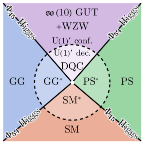
Figure 11: Follow Fig. 8, here we show the same phase diagram in the presence of the WZW term if its low energy consequence is the fermionic parton theory QED${}^{\prime}_{4}$ (Sec. 3.4.2). The dashed circle denotes the confine-deconfine phase transition of the emergent ${\rm U}(1)^{\prime}$ gauge field. The solid-line phase boundaries between two neighbor phases all are described by GUT-Higgs condensation continuous phase transitions. The SM^∗ phase means a modification of SM plus additional BSM fields due to QED${}^{\prime}_{4}$, within the ${\rm U}(1)^{\prime}$ deconfined region inside the dashed circle. Similar situations for GG^∗ and PS^∗.

4d boundary criticality and a 5d bulk bosonic invertible TQFT: Notice that we can interpret the above 4d criticality as a boundary criticality with the $w_{2}w_{3}$ anomaly on the 5d bulk of a mod 2 class invertible TQFT. The 4d WZW, that can be built from the GUT-Higgs fields, can saturate 4d $w_{2}w_{3}(TM)=w_{2}w_{3}(V_{\rm SO(10)})$ anomaly. So we only require the 5d bulk as some 5d invertible topological order or symmetry-protected topological states (SPTs) if we require an onsite Spin(10) symmetry on the 4d boundary and on the 5d bulk; see an overview of modern quantum matter terminology and definitions in [77, 78].

Bosonic UV completion: For this 16n Weyl fermion models, once the $[{\rm Spin}(10)]\supset[\mathbb{Z}_{2}^{F}]$ is dynamically gauged, the whole UV completion of the full 4d and 5d system requires only the bosons, as the local onsite Hilbert space with gauge-invariant bosonic operators.

Although above we focus on the 16n-Weyl-fermion SMs or GUTs, we can consider the 15n-Weyl-fermion models, especially for the $su(5)$ GUT and the SM + 4d WZW term, see Sec. 4.2.

4.2 16n vs 15n Weyl fermions: Give “mass” to “right-handed sterile” neutrinos, canceling mod 2 and mod 16 anomalies, and topological quantum criticality

Although we mostly focus on the 16n-Weyl-fermion SMs or GUTs in this work, here we comment about several ways to obtain the low-energy 15n-Weyl-fermion models (since the real-world experiments only observed the 15n-Weyl-fermion so far) by giving a large mass to the 16th Weyl fermions, the so-called “right-handed sterile” neutrinos (in any of the 3 generation of leptons).

What are examples of conventional ways [41] to give a large (Anderson-Higgs type quadratic) mass to the 16th Weyl fermions? We can pair Weyl fermion to itself (i.e., Majorana mass) or to another Weyl fermion (e.g., Dirac mass):

1. Introduce a Higgs $\Phi_{so(10),\bf 126}$ which can be paired with $\overline{\bf 126}$ out of two Weyl fermions in ${\bf 16}\otimes{\bf 16}={\bf 10}\oplus{\bf 120}\oplus\overline{\bf 126}$.

2. Introduce a Higgs $\Phi_{so(10),\bf 16}$ and add an extra Weyl fermion (17th Weyl fermion) singlet ${\bf 1}$ under Spin(10). This works only if some of the following holds:

   1. The 17th Weyl fermion is not charged under the $\mathbb{Z}_{4,X}$-symmetry, so we have the $\mathbb{Z}_{16}$-anomaly cancelled already by 16n Weyl fermions. This is likely to be true because this 17th Weyl fermion is singlet ${\bf 1}$ under Spin(10), thus is also not acted by the center $Z({\rm Spin}(10))=\mathbb{Z}_{4,X}$.

   2. If the 17th Weyl fermion is also charged under the $\mathbb{Z}_{4,X}$-symmetry, then we require the $\mathbb{Z}_{4,X}$-symmetry is broken (thus the $\mathbb{Z}_{16}$-anomaly is removed), or the $\mathbb{Z}_{4,X}$-symmetry is preserved but $17\mod 16$-anomaly is cancelled again by additional new sectors with $-1\mod 16$-anomaly.

What are other new ways to leave only the observed 15n Weyl fermions at low energy, but the $\mathbb{Z}_{16}$ global anomaly can still be cancelled in the full quantum system? To begin with, to characterize the full 4d anomaly of this 15n SMs or GUTs, we should combine the two types of anomalies: First, a potential global $\mathbb{Z}_{2}$ anomaly, the $w_{2}w_{3}$ for our 4d WZW term, such as in the Fragmentary GUT-Higgs Liquid model in Sec. 3.4. Second, the $\mathbb{Z}_{16}$ global anomaly captured by a 5d version of Atiyah-Patodi-Singer (APS) eta invariant for the ${\rm Spin}\times_{\mathbb{Z}_{2}^{F}}\mathbb{Z}_{4,X}$-structure from $\mathrm{TP}_{5}({\rm Spin}\times_{\mathbb{Z}_{2}^{F}}\mathbb{Z}_{4,X})=\mathbb{Z}_{16}$. We can write that 5d APS invariant in terms of the 4d APS invariant of $\mathrm{Pin}^{+}$-structure from $\mathrm{TP}_{4}(\mathrm{Pin}^{+})=\mathbb{Z}_{16}$. The two combined invertible TQFT, labeled by ${\rm p}\in\mathbb{Z}_{2}$ and $\upnu\in\mathbb{Z}_{16}$, has a partition function ${\bf Z}$ on $M^{5}$, which together labels a deformation class of SM [16]:

$${{\bf Z}_{{\text{$5$d-iTQFT}}}^{({\rm p},\upnu)}}\equiv\exp(\hskip 1.0pt\mathrm{i}\hskip 1.0pt\pi\cdot{\rm p}\cdot\int_{M^{5}}w_{2}w_{3})\cdot\exp(\frac{2\pi\hskip 1.0pt\mathrm{i}\hskip 1.0pt}{16}\cdot\upnu\cdot\eta(\text{PD}({\cal A}_{{\mathbb{Z}_{2}}}))\bigg{\rvert}_{M^{5}}),\\ \text{ with }{\rm p}\in\mathbb{Z}_{2},\quad\text{a 4d Atiyah-Patodi-Singer $\eta$ invariant}\equiv\eta_{\text{Pin}^{+}}\in\mathbb{Z}_{16},\quad\upnu\in\mathbb{Z}_{16}.\;$$ (4.1)

The cohomology classes of background gauge field ${\cal A}_{{\mathbb{Z}_{2}}}\in\operatorname{H}^{1}(M,\frac{\mathbb{Z}_{4,X}}{\mathbb{Z}_{2}^{F}})$ is defined on a ${{\rm Spin}\times_{\mathbb{Z}_{2}^{F}}{\mathbb{Z}_{4,X}}}$-manifold $M$ obeys a constraint: $w_{2}(TM)={\cal A}_{{\mathbb{Z}_{2}}}^{2}$.

Inspired by highly-entangled interacting quantum matter recent developments (see reviews in [77, 78]), Ref. [36, 37, 38] proposed additional new sectors to cancel the anomalies, for example,

1. Symmetry-preserving anomalous gapped 4d TQFT.

2. Symmetric-preserving 5d invertible TQFT in the extra dimension.

3. Symmetry-breaking gapped phase of Landau-Ginzburg kinds.

4. Symmetry-preserving (or breaking) 5d topological gravity theory.

5. Symmetry-preserving or symmetry-breaking gapless phase, e.g., extra massless theories, free or interacting conformal field theories (CFTs). The interacting CFT can also be related to unparticle physics [79] in the high-energy phenomenology community.

The heavy gapped new sectors above can be heavy Dark Matter candidates. The interesting constraints from mod 2 and mod 16 global anomalies on our 4d DQC model are:

• $\mathbb{Z}_{16}$ anomaly constraints on the GG and SM of 15n Weyl fermions: On the Georgi-Glashow $su(5)$ GUT and the Standard Model SM_q=6 side, we can have 15n Weyl fermions, plus additional new sectors enlisted (above and in [36, 37, 38]) to match the $\mathbb{Z}_{16}$ anomaly.

• $\mathbb{Z}_{2}$ $w_{2}w_{3}$ anomaly constraints on the $so(10)$ GUT and PS of 16n Weyl fermions: On the $so(10)$ GUT and the Pati-Salam model sides, there are various types of $\mathbb{Z}_{2}$ class $w_{2}w_{3}$ anomalies, of the ${\rm SO}(10)$, ${\rm SO}(6)$, or ${\rm SO}(4)$ bundles. The $\mathbb{Z}_{2}$ $w_{2}w_{3}$ anomaly is meant to be cancelled by our 4d WZW term.

• At the vicinity of the 4d DQC we have proposed, there can be another interplay between the 15n Weyl fermions (GG and SM) to 16n Weyl fermions (the $so(10)$ GUT and PS), such that the DQC becomes a topological quantum phase transition or topological quantum criticality.

4d boundary criticality to a 5d bulk criticality: Compare with the phase diagram in Fig. 8. Notice that we can interpret the above 4d criticality as a boundary criticality —

• On the modified $so(10)$ GUT and the PS model + WZW term side with 16n Weyl fermions in Fig. 8: with the $w_{2}w_{3}$ $\mathbb{Z}_{2}$-class anomaly on the 5d bulk of a mod 2 class invertible TQFT.

• On the modified $su(5)$ GUT and the SM + WZW term side with 15n Weyl fermions in Fig. 8: with the $\eta(\text{PD}({\cal A}_{{\mathbb{Z}_{2}}}))$ $\mathbb{Z}_{16}$-class anomaly on the 5d bulk of a mod 2 class invertible TQFT.

Once the $[{\rm Spin}(10)]$ is dynamically gauged,

• The 5d bulk on the modified $so(10)$ GUT and the PS model side (16n Weyl fermions): The $[{\rm Spin}(10)]$ dynamical gauge fields can propagate and leak to the 5d bulk are deconfined and gapless.

• The 5d bulk on the modified $su(5)$ GUT and the SM side (15n Weyl fermions): Only the $[\mathbb{Z}_{4,X}]$ subgroup ($Z({\rm Spin}(10))=\mathbb{Z}_{4,X}$) are dynamically gauged in the 5d bulk of the original fermionic invertible TQFT $\eta(\text{PD}({\cal A}_{{\mathbb{Z}_{2}}}))$. Gauging $[\mathbb{Z}_{4,X}]$ turns the 5d fermionic bulk to a 5d bosonic bulk TQFT (with long-range entanglement, gapped topological order, and described by gauged cohomology, gauged cobordism, or higher category theory). The 5d bulk can remain to be gapped.

Thus there is a phase transition between the deconfined and gapless 5d bulk to another side of gapped 5d bulk. This phase transition can be interpreted as a 5d bulk topological quantum criticality.

5 Acknowledgements

JW thanks Pierre Deligne, Lena Funcke, Jun Hou Fung, Chang-Tse Hsieh, Pavel Putrov, Subir Sachdev, Luuk Stehouwer, David Tong, Zheyan Wan, and Yunqin Zheng for helpful comments. YZY thanks John McGreevy for helpful comments. YZY is supported by a startup fund at UCSD. This work is supported by NSF Grant DMS-1607871 “Analysis, Geometry and Mathematical Physics” and Center for Mathematical Sciences and Applications at Harvard University.

Appendix A Quantum Numbers and Representations of SMs and GUTs in Tables

Here we summarize the representations of “elementary” chiral fermionic particles of quarks and leptons of SMs and GUTs in Tables.

Spacetime symmetry representation

Here Weyl fermions are spacetime Weyl spinors, which we prefer to write all Weyl fermions as

$${\bf 2}_{L}\text{ of }{{\rm Spin}(1,3)}=\rm{SL}(2,{\mathbb{C}})$$ (A.1)

with a complex representation in the 4d Lorentz signature. On the other hand, the Weyl spinor is

$${\bf 2}_{L}\text{ of }{\rm Spin}(4)={\rm SU}(2)_{L}\times{\rm SU}(2)_{R}$$ (A.2)

with a pseudoreal representation in the 4d Euclidean signature.

Internal symmetry representation

Below we provide two Tables, 3 and 4, to organize the internal symmetry representations of particle contents of the SM, the $su(5)$ GUT, the Pati-Salam model, the $so(10)$ GUT.

A.1 Embed the SM into the $su(5)$ GUT, then into the $so(10)$ GUT

There is a QFT embedding, the $so(10)$ GUT $\supset$ the $su(5)$ GUT $\supset$ the SM₆ only for $G_{{\rm SM}_{q=6}}$ via an internal symmetry group embedding:

$${{\rm Spin}(10)}\supset G_{\mathrm{GG}}\equiv{\rm SU}(5)\supset G_{{\rm SM}_{6}}\equiv\frac{{{\rm SU}(3)}_{c}\times{{\rm SU}(2)}_{\rm L}\times{\rm U}(1)_{\tilde{Y}}}{\mathbb{Z}_{6}}.$$ (A.3)

The representations of quarks and leptons for these models are organized in Table 3. There are two versions of electroweak hypercharge normalization listed in Table 3, such that the charge of ${\rm U}(1)_{Y}$ is $\frac{1}{6}$ of the charge of ${\rm U}(1)_{\tilde{Y}}$.

$\begin{array}[]{c}\textbf{SM}\\ \textbf{fermion}\\ \textbf{spinor}\\ \textbf{field}\end{array}$ ${{\rm SU}(3)}$ ${{\rm SU}(2)}$ ${\rm U}(1)_{Y}$ ${\rm U}(1)_{\tilde{Y}}$ ${\rm U}(1)_{\rm{EM}}$ ${\rm U}(1)_{{\mathbf{B}-\mathbf{L}}}$ ${\rm U}(1)_{X}$ $\mathbb{Z}_{5,X}$ $\mathbb{Z}_{4,X}$ $\mathbb{Z}_{2}^{F}$ SU(5) Spin(10) $\bar{d}_{R}$ $\overline{\mathbf{3}}$ $\mathbf{1}$ 1/3 2 1/3 $-1/3$ $-3$ $-3$ 1 1 $\overline{\bf{5}}$ ${\bf{16}}$ $l_{L}$ $\mathbf{1}$ $\mathbf{2}$ $-1/2$ $-3$ 0 or $-1$ $-1$ $-3$ $-3$ 1 1 $q_{L}$ ${{\mathbf{3}}}$ $\mathbf{2}$ 1/6 1 2/3 or $-1/3$ 1/3 1 1 1 1 ${\bf{10}}$ $\bar{u}_{R}$ $\overline{\mathbf{3}}$ $\mathbf{1}$ $-2/3$ $-4$ $-2/3$ $-1/3$ 1 $1$ 1 1 $\bar{e}_{R}=e_{L}^{+}$ $\mathbf{1}$ $\mathbf{1}$ 1 6 1 1 1 1 1 1 $\bar{\nu}_{R}={\nu}_{L}$ $\mathbf{1}$ $\mathbf{1}$ 0 0 0 1 5 0 1 1   ${\bf{1}}$

Table 3: Embed the $su(3)\times su(2)\times u(1)$ SM into the Georgi-Glashow $su(5)$ GUT, then into the $so(10)$ GUT. We show the quantum numbers of $15+1=16$ left-handed Weyl fermion (spacetime spinors ${\bf 2}_{L}$ in ${\rm Spin}(1,3)$) in each of three generations of matter fields in SM. The $15$ of 16 Weyl fermion are $\overline{\bf 5}\oplus{\bf 10}$ of SU(5); namely, $(\overline{\bf 3},{\bf 1},1/3)_{L}\oplus({\bf 1},{\bf 2},-1/2)_{L}\sim\overline{\bf 5}$ and $({\bf 3},{\bf 2},1/6)_{L}\oplus(\overline{\bf 3},{\bf 1},-2/3)_{L}\oplus({\bf 1},{\bf 1},1)_{L}\sim{\bf 10}$ of SU(5). The $1$ of 16 is presented neither in the standard GSW SM nor in the $su(5)$ GUT, but it is within ${\bf 16}$ of the $so(10)$ GUT. The numbers in the Table entries indicate the quantum numbers associated with the representation of the groups given in the top row. We show a generation of SM fermion matter fields in Table 3. There are 3 generations, triplicating Table 3, in SM. All fermions have the fermion parity $\mathbb{Z}_{2}^{F}$ representation charge 1. In the $su(5)$ GUT, by including the ${\rm U}(1)_{X}$, we have the $({\rm SU}(5)\times{\rm U}(1)_{X})/\mathbb{Z}_{5}={\rm U}(5)_{\hat{q}=2}$ structure described in Ref. [60, 61]. Here ${\rm U}(1)_{X}\supset\mathbb{Z}_{4,X}\supset\mathbb{Z}_{2}^{F}$ and ${\rm SU}(5)\supset{\rm U}(1)_{Y}$. Both ${\rm U}(1)_{X}$ and ${\rm U}(1)_{{\mathbf{B}-\mathbf{L}}}$ are outside the ${\rm SU}(5)$.

A.2 Embed the SM into the Left-Right and Pati-Salam models, into the $so(10)$ GUT

There are two version of internal symmetry groups for Pati-Salam (PS) model [6]:

$$G_{\mathrm{PS}_{q^{\prime}}}\equiv\frac{{\rm SU}(4)\times{\rm SU}(2)_{\rm L}\times{\rm SU}(2)_{\rm R}}{\mathbb{Z}_{q^{\prime}}}\equiv\frac{{\rm Spin}(6)\times{\rm Spin}(4)}{\mathbb{Z}_{q^{\prime}}}$$

with $q^{\prime}=1,2$. There are two version of internal symmetry groups for Senjanovic-Mohapatra’s Left-Right (LR) model [80],

$$G_{\mathrm{LR}_{q^{\prime}}}\equiv\frac{{{\rm SU}(3)}_{c}\times{{\rm SU}(2)}_{\rm L}\times{{\rm SU}(2)}_{\rm R}\times{\rm U}(1)_{\frac{\mathbf{B}-\mathbf{L}}{2}}}{\mathbb{Z}_{3q^{\prime}}}$$

with $q^{\prime}=1,2$. In general, there is a QFT embedding, the PS model $\supset$ the LR model $\supset$ the SM for both $q^{\prime}=1,2$ via the internal symmetry group embedding:

$$G_{\mathrm{PS}_{q^{\prime}}}\supset G_{\mathrm{LR}_{q^{\prime}}}\supset G_{{\rm SM}_{q=3q^{\prime}}}\equiv\frac{{{\rm SU}(3)}_{c}\times{{\rm SU}(2)}_{\rm L}\times{\rm U}(1)_{\tilde{Y}}}{\mathbb{Z}_{q=3q^{\prime}}}.$$ (A.4)

Namely, when $q^{\prime}=1$, we have

$$G_{\mathrm{PS}_{1}}\supset G_{\mathrm{LR}_{1}}\supset G_{{\rm SM}_{3}}.$$ (A.5)

Furthermore, only when $q^{\prime}=2$, we can have the whole embedded into the Spin(10) for the $so(10)$ GUT:

$${{\rm Spin}(10)}\supset G_{\mathrm{PS}_{2}}\supset G_{\mathrm{LR}_{2}}\supset G_{{\rm SM}_{6}}.$$ (A.6)

The representations of quarks and leptons for these models are organized in Table 4.

$\begin{array}[]{c}\textbf{SM}\\ \textbf{fermion}\\ \textbf{spinor}\\ \textbf{field}\end{array}$ ${{\rm SU}(3)}$ ${{\rm SU}(2)}_{\rm L}$ ${{\rm SU}(2)}_{\rm R}$ ${\rm U}(1)_{\frac{\mathbf{B}-\mathbf{L}}{2}}$ ${\rm U}(1)_{Y}$ ${\rm U}(1)_{Y_{R}}$ ${\rm U}(1)_{\rm{EM}}$ ${\rm U}(1)_{X}$ $\mathbb{Z}_{4,X}$ $\mathbb{Z}_{2}^{F}$ Spin(10) $u_{L}$ ${{\mathbf{3}}}$ $q_{L}:\mathbf{2}$ $\mathbf{1}$ 1/6 1/6 2/3 2/3 1 1 1 ${\bf{16}}$ $d_{L}$ ${{\mathbf{3}}}$ $\mathbf{1}$ 1/6 1/6 $-1/3$ $-1/3$ 1 1 1 $\nu_{L}$ $\mathbf{1}$ $l_{L}:\mathbf{2}$ $\mathbf{1}$ $-1/2$ $-1/2$ 0 0 $-3$ 1 1 $e_{L}$ $\mathbf{1}$ $\mathbf{1}$ $-1/2$ $-1/2$ $-1$ $-1$ $-3$ 1 1 $\bar{u}_{R}$ $\bar{\mathbf{3}}$ $\mathbf{1}$ $q_{R}:\mathbf{2}$ $-1/6$ $-2/3$ $-1/6$ $-2/3$ $1$ 1 1 $\bar{d}_{R}$ $\bar{\mathbf{3}}$ $\mathbf{1}$ $-1/6$ 1/3 $-1/6$ 1/3 $-3$ 1 1 $\bar{\nu}_{R}={\nu}_{L}$ $\mathbf{1}$ $\mathbf{1}$ $l_{R}:\mathbf{2}$ 1/2 0 1/2 0 5 1 1 $\bar{e}_{R}=e_{L}^{+}$ $\mathbf{1}$ $\mathbf{1}$ 1/2 1 1/2 1 1 1 1

Table 4: Embed the $su(3)\times su(2)\times u(1)$ SM into the Pati-Salam ${su(4)\times su(2)\times su(2)}$, then into the $so(10)$ GUT. We have $T_{3,\rm{L}}+Y=Q_{\rm{EM}}$, the Lie algebra linear combination ${{\rm SU}(2)}_{\rm L}$ (the third generator) and ${\rm U}(1)_{Y}$ gives the ${\rm U}(1)_{\rm{EM}}$ charge. We have $T_{3,\rm{R}}+Y=\frac{\mathbf{B}-\mathbf{L}}{2}$, the Lie algebra linear combination of ${{\rm SU}(2)}_{\rm R}$ (the third generator) and ${\rm U}(1)_{Y}$ gives the ${\rm U}(1)_{\mathbf{B}-\mathbf{L}}$. We choose the right-handed anti-particle to be in $\mathbf{2}$ of ${{\rm SU}(2)}_{\rm R}$ (so its right-handed particle to be in $\bar{\mathbf{2}}$ of ${{\rm SU}(2)}_{\rm R}$) that makes a specific assignment on the $\pm$ sign of its $T_{3,{\rm R}}$ charge. So we have the formula, $T_{3,{\rm L}}-T_{3,{\rm R}}=Q_{\rm{EM}}-\frac{\mathbf{B}-\mathbf{L}}{2}$.

Appendix B Representation and Branching Rule for GUT-Higgs symmetry breaking

Here are we organize the set of branching rules of representations following the symmetry breaking pattern of various GUTs to SM (these rules are used in Sec. 2.1):

1. ${\rm Spin}(10)\hookleftarrow{\rm SU}(5)\hookleftarrow\frac{{{\rm SU}(3)}_{c}\times{{\rm SU}(2)}_{\rm L}\times{\rm U}(1)_{Y}}{\mathbb{Z}_{6}}$ branching rules:
   $\diamond$ For ${\rm Spin}(10)\hookleftarrow{\rm SU}(5)$, also for ${\rm SO}(10)\hookleftarrow{\rm U}(5)_{\hat{q}=1}=\frac{{\rm SU}(5)\times{\rm U}(1)_{\hat{q}=1}}{\mathbb{Z}_{5}}$ or ${\rm Spin}(10)\hookleftarrow{\rm U}(5)_{\hat{q}=2}=\frac{{\rm SU}(5)\times{\rm U}(1)_{\hat{q}=2}}{\mathbb{Z}_{5}}$ (or in terms of Lie algebra $so(10)\hookleftarrow{su(5)\times u(1)}$ with a regular Lie subalgebra in [56]), the branching rule says:

   $$\left\{\begin{array}[]{l c l}{\bf 10}\sim{\bf 5}\oplus{\overline{\bf 5}}&\text{or}&{\bf 10}\sim{\bf 5}_{2}\oplus{\overline{\bf 5}}_{-2}.\\ {\bf 16}\sim{\bf 1}\oplus{\overline{\bf 5}}\oplus{\bf 10}&\text{or}&{\bf 16}\sim{\bf 1}_{-5}\oplus{\overline{\bf 5}}_{3}\oplus{\bf 10}_{-1}.\\ {\bf 45}\sim{\bf 1}\oplus{\bf 10}\oplus{\overline{\bf 10}}\oplus{\bf 24}&\text{or}&{\bf 45}\sim{\bf 1}_{0}\oplus{\bf 10}_{4}\oplus{\overline{\bf 10}}_{-4}\oplus{\bf 24}_{0}.\\ {\bf 54}\sim{\bf 15}\oplus{\overline{\bf 15}}\oplus{\bf 24}&\text{or}&{\bf 54}\sim{\bf 15}_{4}\oplus{\overline{\bf 15}}_{-4}\oplus{\bf 24}_{0}.\\ {\bf 120}\sim{\bf 5}\oplus\overline{\bf 5}\oplus{\bf 10}\oplus\overline{\bf 10}\oplus{\bf 45}\oplus\overline{\bf 45}&\text{or}&{\bf 5}_{2}\oplus\overline{\bf 5}_{-2}\oplus{\bf 10}_{-6}\oplus\overline{\bf 10}_{6}\oplus{\bf 45}_{2}\oplus\overline{\bf 45}_{-2}.\\ {\bf 126}\sim{\bf 1}\oplus{\bf 5}\oplus\overline{\bf 10}\oplus{\bf 15}\oplus\overline{\bf 45}\oplus{\bf 50}&\text{or}&{\bf 1}_{10}\oplus{\bf 5}_{2}\oplus\overline{\bf 10}_{6}\oplus{\bf 15}_{-6}\oplus\overline{\bf 45}_{-2}\oplus{\bf 50}_{2}.\end{array}\right.$$ (B.7)

   $\diamond$ For ${\rm SU}(5)\hookleftarrow\frac{{{\rm SU}(3)}_{c}\times{{\rm SU}(2)}_{\rm L}\times{\rm U}(1)_{Y}}{\mathbb{Z}_{6}}$ (or in terms of Lie algebra $su(5)\hookleftarrow{su(3)\times su(2)\times u(1)}$ with a regular Lie subalgebra in [56]), the branching rule says:

   $$\left\{\begin{array}[]{l }{\bf 5}\sim({\bf 1},{\bf 2})_{-3}\oplus({\bf 3},{\bf 1})_{2}.\\ {\bf 10}\sim({\bf 1},{\bf 1})_{-6}\oplus(\overline{\bf 3},{\bf 1})_{4}\oplus({\bf 3},{\bf 2})_{-1}.\\ {\bf 15}\sim({\bf 1},{\bf 3})_{-6}\oplus({\bf 3},{\bf 2})_{-1}\oplus({\bf 6},{\bf 1})_{4}.\\ {\bf 24}\sim({\bf 1},{\bf 1})_{0}\oplus({\bf 1},{\bf 3})_{0}\oplus({\bf 3},{\bf 2})_{5}\oplus(\overline{\bf 3},{\bf 2})_{-5}\oplus({\bf 8},{\bf 1})_{0}.\\ \dots\\ {\bf 45}\sim({\bf 1},{\bf 2})_{-3}\oplus({\bf 3},{\bf 1})_{2}\oplus(\overline{\bf 3},{\bf 1})_{-8}\oplus(\overline{\bf 3},{\bf 2})_{7}\oplus({\bf 3},{\bf 3})_{2}\oplus(\overline{\bf 6},{\bf 1})_{2}\oplus({\bf 8},{\bf 2})_{-3}.\\ {\bf 50}\sim({\bf 1},{\bf 1})_{12}\oplus({\bf 3},{\bf 1})_{2}\oplus(\overline{\bf 3},{\bf 2})_{7}\oplus({\bf 6},{\bf 1})_{-8}\oplus(\overline{\bf 6},{\bf 3})_{2}\oplus({\bf 8},{\bf 2})_{-3}.\\ \end{array}\right.$$ (B.15)

   (1) First, in order to break the Spin(10) or SO(10) down to SU(5), we take the representation whose branching rule in (B.7) contains the ${\bf 1}$ of SU(5) or ${\bf 1}_{0}$ of U(5) on the right-handed side so that SU(5) or U(5) is left unbroken. This means that we may take a GUT-Higgs ${\bf 45}$ that we name it as (2.23):

   $$\Phi_{so(10),\bf 45}\equiv\Phi_{\bf 45}.$$ (B.16)

   (2) Second, in order to break SU(5) further down to $G_{{\rm SM}_{6}}\equiv\frac{{{\rm SU}(3)}_{c}\times{{\rm SU}(2)}_{\rm L}\times{\rm U}(1)_{Y}}{\mathbb{Z}_{6}}$, we take the representation whose branching rule in (B.15) contains the $({\bf 1},{\bf 1})_{0}$ of $G_{{\rm SM}_{6}}$. This means that we can take the ${\bf 24}$ of SU(5) as the second GUT-Higgs called $\Phi_{su(5),\bf 24}$. But if we want to obtain this second GUT-Higgs from a higher-energy $so(10)$ GUT, it turns out that we can find $\Phi_{su(5),\bf 24}$ within (2.24):

   $$\Phi_{so(10),\bf 54}\equiv\Phi_{\bf 54},$$ (B.17)

   from (B.7) more naturally, as we will soon see.

2. ${\rm Spin}(10)\hookleftarrow\frac{{\rm Spin}(6)\times{\rm Spin}(4)}{\mathbb{Z}_{2}}\hookleftarrow\frac{{{\rm SU}(3)}_{c}\times{{\rm SU}(2)}_{\rm L}\times{\rm U}(1)_{Y}}{\mathbb{Z}_{6}}$ branching rules:
   $\diamond$ For ${\rm Spin}(10)\hookleftarrow\frac{{\rm Spin}(6)\times{\rm Spin}(4)}{\mathbb{Z}_{2}}=\frac{{\rm SU}(4)\times{\rm SU}(2)\times{\rm SU}(2)}{\mathbb{Z}_{2}}$, also for ${\rm SO}(10)\hookleftarrow{{\rm SO}(6)\times{\rm SO}(4)}$ (or in terms of Lie algebra $so(10)\hookleftarrow{so(6)\times so(4)}$ or ${su(4)\times su(2)\times su(2)}$ with a regular Lie subalgebra in [56]), we find that:

   $$\left\{\begin{array}[]{l }{\bf 10}\sim({\bf 1},{\bf 2},{\bf 2})\oplus({\bf 6},{\bf 1},{\bf 1}).\\ {\bf 16}\sim({\bf 4},{\bf 2},{\bf 1})\oplus(\overline{\bf 4},{\bf 1},{\bf 2}).\\ {\bf 45}\sim({\bf 1},{\bf 3},{\bf 1})\oplus({\bf 1},{\bf 1},{\bf 3})\oplus({\bf 6},{\bf 2},{\bf 2})\oplus({\bf 15},{\bf 1},{\bf 1}).\\ {\bf 54}\sim({\bf 1},{\bf 1},{\bf 1})\oplus({\bf 1},{\bf 3},{\bf 3})\oplus({\bf 6},{\bf 2},{\bf 2})\oplus({\bf 20}^{\prime},{\bf 1},{\bf 1}).\\ {\bf 120}\sim({\bf 1},{\bf 2},{\bf 2})\oplus({\bf 6},{\bf 3},{\bf 1})\oplus({\bf 6},{\bf 1},{\bf 3})\oplus({\bf 10},{\bf 1},{\bf 1})\oplus(\overline{\bf 10},{\bf 1},{\bf 1})\oplus({\bf 15},{\bf 2},{\bf 2}).\\ {\bf 126}\sim({\bf 6},{\bf 1},{\bf 1})\oplus(\overline{\bf 10},{\bf 3},{\bf 1})\oplus({\bf 10},{\bf 1},{\bf 3})\oplus({\bf 15},{\bf 2},{\bf 2}).\end{array}\right.$$ (B.24)

   $\diamond$ For $\frac{{\rm Spin}(6)\times{\rm Spin}(4)}{\mathbb{Z}_{2}}=\frac{{\rm SU}(4)\times{\rm SU}(2)\times{\rm SU}(2)}{\mathbb{Z}_{2}}\hookleftarrow\frac{{{\rm SU}(3)}_{c}\times{{\rm SU}(2)}_{\rm L}\times{\rm U}(1)_{Y}}{\mathbb{Z}_{6}}$ (or in terms of Lie algebra ${so(6)\times so(4)}$ or ${su(4)\times su(2)\times su(2)}\hookleftarrow{su(3)\times su(2)\times u(1)}$), we find that the $su(4)\hookleftarrow{su(3)\times u(1)}$ (with a regular Lie subalgebra in [56]) branching rule says:

   $$\left\{\begin{array}[]{l }{\bf 4}\sim{\bf 1}_{-3}\oplus{\bf 3}_{1}.\\ {\bf 6}\sim{\bf 3}_{-2}\oplus\overline{\bf 3}_{2}.\\ {\bf 10}\sim{\bf 1}_{-6}\oplus{\bf 3}_{-2}\oplus{\bf 6}_{2}.\\ {\bf 15}\sim{\bf 1}_{0}\oplus{\bf 3}_{4}\oplus\overline{\bf 3}_{-4}\oplus{\bf 8}_{0}.\end{array}\right.$$ (B.29)

   (1) First, in order to break the Spin(10) down to $G_{\mathrm{PS}_{2}}\equiv\frac{{\rm Spin}(6)\times{\rm Spin}(4)}{\mathbb{Z}_{2}}=\frac{{\rm SU}(4)\times{\rm SU}(2)\times{\rm SU}(2)}{\mathbb{Z}_{2}}$, we take the representation whose branching rule in (B.24) contains the $({\bf 1},{\bf 1},{\bf 1})$ on the right-handed side so that $G_{\mathrm{PS}_{2}}$ is left unbroken. This means that we may take a GUT-Higgs ${\bf 54}$ that we had named it in (2.24) as

   $$\Phi_{so(10),\bf 54}\equiv\Phi_{\bf 54}.$$

   (2) Second, in order to break $G_{\mathrm{PS}_{2}}$ further down to $G_{{\rm SM}_{6}}\equiv\frac{{{\rm SU}(3)}_{c}\times{{\rm SU}(2)}_{\rm L}\times{\rm U}(1)_{Y}}{\mathbb{Z}_{6}}$, we take the representation whose branching rule in (B.15) contains the $({\bf 1},{\bf 1})_{0}$ of $G_{{\rm SM}_{6}}$. This means that we can take the ${\bf 15}$ of SU(4) as the second GUT-Higgs called $\Phi_{su(4),\bf 15}$. But if we want to obtain this second GUT-Higgs from a higher-energy $so(10)$ GUT, it turns out that we can find $\Phi_{su(4),\bf 15}$ from what we had named in (2.23) called

   $$\Phi_{so(10),\bf 45}\equiv\Phi_{\bf 45},$$

   from (B.24) more naturally, as we will soon see.

3. $\frac{{{\rm SU}(3)}_{c}\times{{\rm SU}(2)}_{\rm L}\times{\rm U}(1)_{Y}}{\mathbb{Z}_{6}}\hookleftarrow\frac{{{\rm SU}(3)}_{c}\times{\rm U}(1)_{\rm{EM}}}{\mathbb{Z}_{3}}$ branching rules:
   The Standard Model (SM) electroweak Higgs in the representation

   $$\Phi_{{\rm SM}}\text{ in }({\bf 1},{\bf 2})_{Y=\frac{1}{2}}=({\bf 1},{\bf 2})_{Y_{W}={1}}=({\bf 1},{\bf 2})_{\tilde{Y}={3}}\text{ of }su(3)\times su(2)\times u(1)$$ (B.30)

   does the job to break $G_{{\rm SM}_{6}}\equiv\frac{{{\rm SU}(3)}_{c}\times{{\rm SU}(2)}_{\rm L}\times{\rm U}(1)_{Y}}{\mathbb{Z}_{6}}$ to $\frac{{{\rm SU}(3)}_{c}\times{\rm U}(1)_{\rm{EM}}}{\mathbb{Z}_{3}}$. Then next, we can ask how to find $\Phi_{{\rm SM}}$ from the representation of $su(5)$, or ${su(4)\times su(2)\times su(2)}$, or $so(10)$.

   $\bullet$ $\Phi_{{\rm SM}}$ from $su(5)$: From the branching rule in (B.15), one can try to take the $\Phi_{su(5),\bf 5}$ and $\Phi_{su(5),\bf 45}$ which contains $({\bf 1},{\bf 2})_{-{3}}$ of ${su(3)\times su(2)\times u(1)}$ which is the complex conjugation of $\Phi_{{\rm SM}}$’s $({\bf 1},{\bf 2})_{\tilde{Y}={3}}$.

   $\bullet$ $\Phi_{{\rm SM}}$ from ${su(4)\times su(2)\times su(2)}$: From the branching rule in (B.29), one can try to take the $\Phi_{{su(4)\times su(2)\times su(2)},({\bf 4},{\bf 2},{\bf 1})}$ that contains $({\bf 1},{\bf 2})_{-{3}}$ of ${su(3)\times su(2)\times u(1)}$, which is also the complex conjugation of $\Phi_{{\rm SM}}$’s $({\bf 1},{\bf 2})_{\tilde{Y}={3}}$. We may also need $\Phi_{{su(4)\times su(2)\times su(2)},(\overline{\bf 4},{\bf 1},{\bf 2})}$ if we wish to break the ${\rm SU}(2)_{\rm R}$ completely.

   $\bullet$ $\Phi_{{\rm SM}}$ from $so(10)$:
   From the branching rule in (B.7), we can get the $\Phi_{su(5),\bf 5}$ and $\Phi_{su(5),\bf 45}$ out of ${\bf 10}$, ${\bf 120}$ or $\overline{\bf 126}$ of $so(10)$, which we can call $\Phi_{so(10),\bf 10}$, $\Phi_{so(10),\bf 120}$, and $\Phi_{so(10),\overline{\bf 126}}$. These ${\bf 10}$, ${\bf 120}$ or $\overline{\bf 126}$ are particular sensible according to [41], because these Higgs can be paired up with the fermion bilinear operators $\psi_{i}\psi_{j}$ whose representations are also in the tensor product ${\bf 16}\otimes{\bf 16}={\bf 10}\oplus{\bf 120}\oplus\overline{\bf 126}$.

   From the branching rule in (B.24), we can get the $\Phi_{{su(4)\times su(2)\times su(2)},({\bf 4},{\bf 2},{\bf 1})}$ and $\Phi_{{su(4)\times su(2)\times su(2)},(\overline{\bf 4},{\bf 1},{\bf 2})}$ out of ${\bf 16}$ of Spin(10), which we can call $\Phi_{so(10),\bf 16}$.

Appendix C Induce a 3d WZW term between Néel $so(2)$ and VBS $so(3)$ on a 4d bulk $w_{2}(V_{{\rm SO}(3)})w_{2}(V_{{\rm SO}(2)})$

This Appendix provides a logical pedagogical account on the familiar 3d dQCP [27] proposed as a continuous quantum phase transition, on a 2+1d bosonic lattice model with an internal non-relativistic (iso)spin-1/2 bosons, between two kinds of Landau-Ginzburg symmetry breaking orders on each lattice site:

1. One side has the Néel anti-ferromagnet order: This order breaks the $\mathbb{Z}^{2}$-spatial lattice translation to $(\mathbb{Z}_{2})^{2}$ on a lattice. It also breaks the ${\rm SO}(3)$ internal (iso)spin rotational symmetry (actually, breaking SO(3) faithfully, not SU(2)). But it respects the spatial rotational symmetry, which is $\mathbb{Z}_{4}$ spatial rotational symmetry on a square lattice, but it preserves an enhanced ${\rm SO}(2)$ spatial rotational symmetry in the continuum.

2. Another side has the Valence-Bond Solid (VBS) order, which preserves a faithful ${\rm SO}(3)$ (iso)spin rotational symmetry (again, see footnote 41), because the VBS order pairs the two neighbor-site (iso)spin-1/2 bosons to an (iso)spin-0 state $\frac{1}{\sqrt{2}}(|\uparrow\rangle|\downarrow\rangle-|\downarrow\rangle|\uparrow\rangle)$. But the pattern of VBS breaks the $\mathbb{Z}_{4}$ spatial rotational symmetry on a square lattice, so the VBS breaks an ${\rm SO}(2)$ spatial rotational symmetry in the continuum.

If we take into account the discrete $\mathbb{Z}_{2}$ symmetry (a time-reversal or a spatial reflection symmetry), the above ${\rm SO}(2)$ symmetry becomes an ${\rm O}(2)={\rm SO}(2)\rtimes\mathbb{Z}_{2}$ symmetry, while the above ${\rm SO}(3)$ symmetry becomes an ${\rm O}(3)={\rm SO}(3)\times\mathbb{Z}_{2}$ symmetry.

Below we write $G$ as the original symmetry group (such as ${{\rm SO}(3)\times{\rm SO}(2)}$ valid to the UV lattice scale), while ${G_{\text{sub}}}$ is the remained preserved unbroken symmetry in the corresponding order (Néel or VBS orders). Then we have the following fibration structure:

$${G_{\text{sub}}}\lhook\joinrel\xrightarrow{\quad}G\longrightarrow\frac{G}{G_{\text{sub}}},$$ (C.1)

where the quotient space $\frac{G}{G_{\text{sub}}}$ is the base manifold (i.e., the orbit) as the symmetry-breaking order parameter space. The $G$ is the total space obtained from the fibration of the ${G_{\text{sub}}}$ fiber (i.e., the stabilizer) over the base $\frac{G}{G_{\text{sub}}}$. Here is a systematic table computation on the homotopy group $\pi_{k}$ of $(\frac{G}{G_{\text{sub}}})$ for Néel or VBS orders,

$$\begin{tabular}[]{lccccccc}\hline\cr&$\pi_{0}$&$\pi_{1}$&$\pi_{2}$&$\pi_{3}$&$\pi_{4}$&$\pi_{5}$\\ \hline\cr N\'{e}el $S^{2}=\frac{{\rm O}(3)\times{\rm O}(2)}{{\rm O}(2)\times{\rm O}(2)}=\frac{{\rm O}(3)}{{\rm O}(2)}$&$0$&$0$&$\mathbb{Z}$&$\mathbb{Z}$&$\mathbb{Z}_{2}$&$\mathbb{Z}_{2}$\\ \;\;\,\quad\quad\quad$=\frac{{\rm SO}(3)\times{\rm SO}(2)}{{\rm SO}(2)\times{\rm SO}(2)}=\frac{{\rm SO}(3)}{{\rm SO}(2)}$&&&&&&\\ \hline\cr VBS $S^{1}=\frac{{\rm O}(3)\times{\rm O}(2)}{{\rm O}(3)\times{\rm O}(1)}=\frac{{\rm O}(2)}{{\rm O}(1)}$&$0$&$\mathbb{Z}$&$0$&$0$&$0$&$0$\\ \;\;\,\quad\quad\quad$=\frac{{\rm SO}(3)\times{\rm SO}(2)}{{\rm SO}(3)\times{\rm SO}(1)}=\frac{{\rm SO}(2)}{{\rm SO}(1)}$&&&&&&\\ \hline\cr${\rm O}(5)$&$\mathbb{Z}_{2}$&$\mathbb{Z}_{2}$&$0$&$\mathbb{Z}$&$\mathbb{Z}_{2}$&$\mathbb{Z}_{2}$\\ \hline\cr${\rm SO}(5)$&$0$&$\mathbb{Z}_{2}$&$0$&$\mathbb{Z}$&$\mathbb{Z}_{2}$&$\mathbb{Z}_{2}$\\ \hline\cr\end{tabular}.$$ (C.9)

To our knowledge, the most systematic, physically intuitive, and mathematically transparent construction of the 3d dQCP and its 3d WZW term can be based on the following arguments:

1. The Néel order breaks an ${\rm SO}(3)$ (iso)spin rotational symmetry down to an ${\rm U}(1)={\rm SO}(2)$ (iso)spin rotational symmetry such as along the $z$ axis, such that (3.26) in the Néel order becomes:

   $$\Big{(}{G_{\text{sub}}}={{\rm SO}(2)\times{\rm SO}(2)}\Big{)}\lhook\joinrel\xrightarrow{\quad}\Big{(}G={{\rm SO}(3)\times{\rm SO}(2)}\Big{)}\longrightarrow\Big{(}\frac{G}{G_{\text{sub}}}=S^{2}\Big{)}.$$ (C.10)

   1. Hedgehog core, instanton, and magnetic monopole: The ${\rm SO}(3)$ symmetry breaking hedgehog core has a 0d singularity in the spacetime. This 0d singularity of this hedgehog core in the 3d spacetime can be also regarded an instanton in the 3d spacetime. We can couple this whole configuration to SO(3) background gauge field, this means that we can use the $w_{2}(V_{SO(3)})$ to measure the magnetic charge of SO(3). We evaluate the $w_{2}(V_{SO(3)})$ over the Néel’s SO(3) symmetry-breaking target space $S^{2}$, it turns out that there is a $2\pi$-flux over $S^{2}$. Therefore, the hedgehog core is not only an instanton event but also an SO(3) magnetic monopole, living on a 0d open end of some non-dynamical 1d ’t Hooft line defect of SO(3) background gauge field.

   2. This ${\rm SO}(3)$ symmetry-breaking hedgehog core traps a “fractionalized charge-1/2 object charged under the preserved SO(2) symmetry (or $\mathbb{Z}_{4}$ symmetry on a lattice scale),” namely in the projective representation of $\mathbb{Z}_{4}$, which is in the unit integer representation $\mathbb{Z}_{8}$. Namely, the ${\rm SO}(3)$-symmetry-breaking topological defect, hedgehog core in the Néel phase, traps the $\frac{1}{2}$-fractionalization of the unbroken ${\rm SO}(2)$, or $\mathbb{Z}_{4}$, charged object of VBS order.

   3. The winding number of such Néel hedgehog configuration can be classified by

      $$\pi_{2}(\frac{{\rm SO}(3)\times{\rm SO}(2)}{{\rm SO}(2)\times{\rm SO}(2)})=\pi_{2}(\frac{{\rm SO}(3)}{{\rm SO}(2)})=\pi_{2}(S^{2})=\mathbb{Z}.$$ (C.11)

      This says the $S^{2}$ as a 2d surface in 3d spacetime wrapping around the target $S^{2}$ of the Néel’s SO(3) symmetry-breaking target space (the base manifold and stabilizer in (C.10)). The spatial $S^{2}$ circle as a homology class (in $\operatorname{H}_{2}(M,\mathbb{Z})$, called this 2d sphere $\varrho^{2}_{\text{}}$) can be paired up with a cohomology class ${\cal B}\in\operatorname{H}^{2}(M,\mathbb{Z})$. To make sense the unit generator of the winding $\mathbb{Z}$ class, the ${\cal B}$ evaluated on $\varrho^{2}$ (bounding a 3-disk $\Sigma^{3}$ by $\varrho^{2}$ so $\partial\Sigma^{3}=\varrho^{2}$) must have the following:

      $$\displaystyle\int\mkern-7.0mu\begin{picture}(0.0,3.0)\put(0.0,3.0){\oval(10.0,8.0)}\end{picture}\mkern-8.0mu\int_{\varrho^{2}=\partial\Sigma^{3}}{\cal B}=\displaystyle\int\mkern-7.0mu\begin{picture}(0.0,3.0)\put(0.0,3.0){\oval(10.0,8.0)}\end{picture}\mkern-8.0mu\int_{\varrho^{2}}w_{2}(V_{{\rm SO}(3)})=1\mod 2.$$ (C.12)

   4. Now imagine in a 3d spacetime picture, we can regard:
      $\bullet$ the 0d hedgehog core $\varsigma^{0}_{\text{N\'{e}el hedgehog}}$ as the charged object, fractionalized charged under the preserved SO(2) (a projective representation in $\mathbb{Z}_{4}$, precisely a linear representation in $\mathbb{Z}_{8}$).
      $\bullet$ the 2d $S^{2}$ called $\varrho^{2}_{\text{}}$ with ${\cal B}\in\operatorname{H}^{2}(M,\mathbb{Z})$ on the $\varrho^{2}_{\text{}}$, as the charge operator, or the symmetry generator of the SO(2).
      Then, follow the higher symmetry or generalized global symmetry language [57], the measurement of the symmetry is exactly performed by evaluating the linking between the $\varsigma^{0}_{\text{N\'{e}el hedgehog}}$ and $\varrho^{2}_{\text{}}$ in a 3d spacetime $M^{3}$. Precisely, the linking number Lk, manifested as a statistical Berry phase, is evaluated via the expectation value of path integral:

      $$\langle\exp(\hskip 1.0pt\mathrm{i}\hskip 1.0pt\pi\displaystyle\int\mkern-7.0mu\begin{picture}(0.0,3.0)\put(0.0,3.0){\oval(10.0,8.0)}\end{picture}\mkern-8.0mu\int_{\varrho^{2}=\partial\Sigma^{3}}{\cal B})\cdot\exp(\hskip 1.0pt\mathrm{i}\hskip 1.0pt\pi\varphi\big{|}_{\varsigma^{0}_{\text{N\'{e}el hedgehog}}})\rangle=(-1)^{{\rm Lk}(\varrho^{2},\varsigma^{0}_{\text{N\'{e}el hedgehog}})}\Big{|}_{M^{3}}$$ (C.13)

      Here $\varphi\big{|}_{\varsigma^{0}_{\text{N\'{e}el hedgehog}}}$ is the 0d vertex operator evaluated around the 0d hedgehog core, which is again the 0d magnetic monopole at the open end of the SO(3) background-gauged 1d ’t Hooft line. Related descriptions of link invariants of QFTs can be found in [58, 59] and references therein.

2. The VBS order breaks an ${\rm SO}(2)$ spatial rotational symmetry in the continuum (or breaks $\mathbb{Z}_{4}$ rotational symmetry on a lattice), such that (3.26) in the VBS order becomes:

   $$\Big{(}{G_{\text{sub}}}={{\rm SO}(3)\times{\rm SO}(1)}\Big{)}\lhook\joinrel\xrightarrow{\quad}\Big{(}G={{\rm SO}(3)\times{\rm SO}(2)}\Big{)}\longrightarrow\Big{(}\frac{G}{G_{\text{sub}}}=S^{1}\Big{)}.$$ (C.14)

   1. The ${\rm SO}(2)$ symmetry-breaking VBS vortex core has a 0d singularity trapping an (iso)spin-1/2 object called the (iso)spinon in the space (famously popularized by Levin-Senthil [81]), which indeed is a 1d vortex loop (called this 1d loop $\varsigma^{1}_{\text{VBS vortex}}$) in the spacetime.

   2. The (iso)spinon with (iso)spin-1/2 trapped at the VBS order parameter vortex core is a “fractionalized charge-1/2 object charged under the preserved symmetry SO(3),” namely in the projective representation of SO(3), which is in the fundamental representation 2 of SU(2). Namely, the ${\rm SO}(2)$-symmetry-breaking topological defect, the vortex in the VBS phase, traps the $\frac{1}{2}$-fractionalization of ${\rm SO}(3)$ charged object of Néel order.

   3. The winding number of such VBS vortex configuration can be classified by

      $$\pi_{1}(\frac{{\rm SO}(3)\times{\rm SO}(2)}{{\rm SO}(3)\times{\rm SO}(1)})=\pi_{1}(\frac{{\rm SO}(2)}{{\rm SO}(1)})=\pi_{1}(S^{1})=\mathbb{Z}.$$ (C.15)

      This says the spatial $S^{1}$ wrapping around the target $S^{1}$ of the VBS’s SO(2) symmetry-breaking target space (the base manifold and stabilizer in (C.14)). The spatial $S^{1}$ circle as a homology class (in $\operatorname{H}_{1}(M,\mathbb{Z})$, called this 1d circle $\varrho^{1}_{\text{}}$) can be paired up with a cohomology class ${\cal A}\in\operatorname{H}^{1}(M,\mathbb{Z})$. To make sense the unit generator of the winding $\mathbb{Z}$ class, the $\hskip 1.0pt\mathrm{d}{\cal A}$ evaluated on a 2-disk $\Sigma^{2}$ (bounded by $\varrho^{1}$ so $\partial\Sigma^{2}=\varrho^{1}$) must have the following Stoke theorem:

      $$\oint_{\varrho^{1}=\partial\Sigma^{2}}{\cal A}=\int_{\Sigma^{2}}\hskip 1.0pt\mathrm{d}{\cal A}=\int_{\Sigma^{2}}w_{2}(V_{{\rm SO}(2)})=1\mod 2.$$ (C.16)

   4. Now imagine in a 3d spacetime picture, we can regard:
      $\bullet$ the 1d vortex loop $\varsigma^{1}_{\text{VBS vortex}}$ as the charged object, fractionalized charged under the preserved SO(3) (a projective representation in SO(3), precisely a linear representation in SU(2)).
      $\bullet$ the 1d $S^{1}$ circle $\varrho^{1}_{\text{}}$ with ${\cal A}\in\operatorname{H}^{1}(M,\mathbb{Z})$ on the loop, as the charge operator, or the symmetry generator of the SO(3).
      Then, the measurement of the symmetry is exactly performed by evaluating the linking between the $\varsigma^{1}_{\text{VBS vortex}}$ and $\varrho^{1}_{\text{}}$ in 3d spacetime. Precisely, the linking number Lk, manifested as a statistical Berry phase, is evaluated via the expectation value of path integral:

      $$\langle\exp(\hskip 1.0pt\mathrm{i}\hskip 1.0pt\pi\oint_{\varrho^{1}=\partial\Sigma^{2}}{\cal A})\cdot\exp(\hskip 1.0pt\mathrm{i}\hskip 1.0pt\pi\oint_{\varsigma^{1}_{\text{VBS vortex}}}a)\rangle=(-1)^{{\rm Lk}(\varrho^{1},\varsigma^{1}_{\text{VBS vortex}})}\Big{|}_{M^{3}}$$ (C.17)

      Here $a$ is a 1d background-gauged ${\rm SO}(2)$ connection evaluated around the 1d vortex loop. Related descriptions of link invariants of QFTs can be found in [58, 59] and references therein.

3. Overall, combined the above data, we have learned that the 3d dQCP construction can be induced by the linking number ${{\rm Lk}(\varrho^{2},\varsigma^{0}_{\text{N\'{e}el hedgehog}})}=1$ and ${{\rm Lk}(\varrho^{1},\varsigma^{1}_{\text{VBS vortex}})}=1$ in the 3d spacetime. To furnish more physical intuitions, we can deduce that:

   1. If we extend the 3d spacetime $t,x,y$ to an extra 4th dimension $z$, the previous 0d hedgehog core $\varsigma^{0}_{\text{N\'{e}el hedgehog}}$ trajectory can be a 1d pseudo-worldline ${\varsigma^{\prime 1}_{\text{N\'{e}el hedgehog}}}$ in the 4d spacetime $M^{4}$. Similarly, the previous 1d vortex loop ${\varsigma^{1}_{\text{VBS vortex}}}$ trajectory can be a 2d pseudo-worldsheet ${\varsigma^{\prime 2}_{\text{VBS vortex}}}$ in the 4d spacetime $M^{4}$. Such two configurations can be linked in 4d, with a linking number:

      $${{\rm Lk}({\varsigma^{\prime 1}_{\text{N\'{e}el hedgehog}}},{\varsigma^{\prime 2}_{\text{VBS vortex}}})}\Big{|}_{M^{4}}.$$ (C.18)

      This describes the link in the extended 4d spacetime of two charged objects, charged under SO(2) and SO(3) respectively.
      

   2. In a parallel story, the charge operators (of the above charged objects) are the 1d SO(2)-background gauged ${\cal A}$ line operator on $\varrho^{1}$, and 2d SO(3)-background gauged ${\cal B}$ surface operator on $\varrho^{2}$. Such two configurations can be linked in 4d, with a linking number:

      $${{\rm Lk}({\cal A}\text{ on }\varrho^{1},{\cal B}\text{ on }\varrho^{2})}\Big{|}_{M^{4}}.$$ (C.19)

      This describes the link in the extended 4d spacetime of two charge operators, of SO(2) and SO(3) respectively.

      $\bullet$ If we open up the closed $\oint_{\varrho^{1}}{\cal A}$ on $\varrho^{1}$ with two open ends on the 3d boundary ${M^{3}}$ of the bulk ${M^{4}}$, then one open end carries a $\varphi\big{|}_{\varsigma^{0}_{\text{N\'{e}el hedgehog}}}$. Their link configuration in 3d corresponds to the earlier (C.13):

      $${{\rm Lk}(\varsigma^{0}_{\text{N\'{e}el hedgehog}},\varrho^{2})}\Big{|}_{M^{3}}.$$

      $\bullet$ If we open up the closed $\displaystyle\int\mkern-7.0mu\begin{picture}(0.0,3.0)\put(0.0,3.0){\oval(10.0,8.0)}\end{picture}\mkern-8.0mu\int_{\varrho^{2}}{\cal B}$ on $\varrho^{2}$ with an open end on the 3d boundary ${M^{3}}$ of the bulk ${M^{4}}$, then this open end carries a closed 1d vortex loop $\oint_{\varsigma^{1}_{\text{VBS vortex}}}a$. Their link configuration in 3d corresponds to the earlier (C.17):

      $${{\rm Lk}(\varsigma^{1}_{\text{VBS vortex}},\varrho^{1})}\Big{|}_{M^{3}}.$$

   These above facts together imply that:

   1. The 3d dQCP construction [27] is valid if we introduce a mod 2 class 3d WZW term defined on a 3d boundary $M^{3}$ of a 4d manifold $M^{4}$. Based on the homotopy data $\pi_{1}(S^{1})=\mathbb{Z}$ and $\pi_{2}(S^{2})=\mathbb{Z}$, schematically the WZW in a differential form or de Rham cohomology is:

      $$\exp(\hskip 1.0pt\mathrm{i}\hskip 1.0ptS^{\text{WZW}})=\exp(\hskip 1.0pt\mathrm{i}\hskip 1.0pt\pi\int_{M^{4}}{\cal A}\wedge\hskip 1.0pt\mathrm{d}{\cal B}).\Big{|}_{{M^{3}=\partial{M^{4}}}}$$ (C.20)

      More precisely, we can improve this to construct the cohomology class relying on ${\cal A}\in\operatorname{H}^{1}(S^{1},\mathbb{Z})=\mathbb{Z}$ and ${\cal B}\in\operatorname{H}^{2}(S^{2},\mathbb{Z})=\mathbb{Z}$ classes, the WZW term is written in the singular cohomology class of ${\cal A}$ and ${\cal B}$:

      $$\exp(\hskip 1.0pt\mathrm{i}\hskip 1.0ptS^{\text{WZW}})=\exp(\hskip 1.0pt\mathrm{i}\hskip 1.0pt\pi\int_{M^{4}}{\cal A}\smile\delta{\cal B})\Big{|}_{{M^{3}=\partial{M^{4}}}}=\exp(\hskip 1.0pt\mathrm{i}\hskip 1.0pt2\pi\int_{M^{4}}{\cal A}\smile\mathrm{Sq}^{1}{\cal B})\Big{|}_{{M^{3}=\partial{M^{4}}}},$$ (C.21)

      with the coboundary operator $\delta$, and the Steenrod square $\mathrm{Sq}^{1}\equiv\frac{\delta}{2}\mod 2$ here maps the singular cohomology $\operatorname{H}^{2}(M,\mathbb{Z}_{2})\mapsto\operatorname{H}^{3}(M,\mathbb{Z}_{2})$, on some triangulable manifold $M$.

   2. The 3d dQCP construction [27] is supported by a 3d ’t Hooft anomaly in the ${{\rm SO}(3)\times{\rm SO}(2)}$ global symmetry on a 3-manifold $M^{3}$, captured by a 4d bulk invertible TQFT [64] living on a 4-manifold $M^{4}$ with a boundary $\partial M^{4}=M^{3}$:

      $$\exp(\hskip 1.0pt\mathrm{i}\hskip 1.0pt\pi\int_{M^{4}}w_{2}(V_{{\rm SO}(3)})w_{2}(V_{{\rm SO}(2)})).$$ (C.22)

      This 3d ’t Hooft anomaly is a mod 2 class global anomaly, whose 4d invertible TQFT corresponds to a $\mathbb{Z}_{2}$ generator in the following cobordism group $\Omega^{d}_{G}\equiv\mathrm{TP}_{d}(G)$ (see the detailed computations in [61]):

      a $$\mathbb{Z}_{2} w_{4}(V_{{\rm SO}(5)}) \mathrm{TP}_{4}({\rm SO}\times{\rm SO}(5))=\mathbb{Z}_{2}$$ generator in , (C.23)

      a $$\mathbb{Z}_{2} w_{2}(V_{{\rm SO}(3)})w_{2}(V_{{\rm SO}(2)})) \mathrm{TP}_{4}({\rm SO}\times{\rm SO}(3)\times{\rm SO}(2))=\mathbb{Z}_{2}$$ generator in . (C.24)

With (C.21) and (C.22), these conclude our derivation of 3d WZW and ’t Hooft anomaly for 3d dQCP for Néel-VBS transition.

Appendix D Perturbative Local and Nonperturbative Global Anomalies via Cobordism: Without or With $T$ or $CP$ symmetry

Here we enlist the results of perturbative local and nonperturbative global anomalies via cobordism mostly obtained from [22, 24]. Some of these results are used in (2.17). For some spacetime-internal symmetry group $\bar{G}$ of the SM or GUT models, we denote:

$$\bar{G}\equiv{{G_{\text{spacetime}}}\times_{{N_{\text{shared}}}}{{G}_{\text{internal}}}}\equiv({\frac{{G_{\text{spacetime}}}\times{{G}_{\text{internal}}}}{{N_{\text{shared}}}}}).$$

We apply a version of cobordism group $\Omega^{d}_{\bar{G}}\equiv\mathrm{TP}_{d}(\bar{G})$ from Freed-Hopkins [26]. Ref. [12, 22, 24, 61] had computed some of these 5th cobordism group $\mathrm{TP}_{5}$ classifications of the 4d anomalies (via Thom-Madsen-Tillmann spectra [82, 83], Adams spectral sequence [84], and Freed-Hopkins’s theorem [26]), to obtain:

$$\mathrm{TP}_{5}({\rm Spin}\times_{\mathbb{Z}_{2}^{F}}\mathbb{Z}_{4,X}\times G_{{\rm SM}_{q}}) = \left\{\begin{array}[]{ll}\mathbb{Z}^{5}\times\mathbb{Z}_{2}\times\mathbb{Z}_{4}^{2}\times\mathbb{Z}_{16},&q=1,3.\\ \mathbb{Z}^{5}\times\mathbb{Z}_{2}^{2}\times\mathbb{Z}_{4}\times\mathbb{Z}_{16},&q=2,6.\end{array}\right.$$ (D.3)

$$\mathrm{TP}_{5}({\rm Spin}\times_{\mathbb{Z}_{2}^{F}}\mathbb{Z}_{4,X}\times{\rm SU}(5)) = \mathbb{Z}\times\mathbb{Z}_{2}\times\mathbb{Z}_{16}.$$ (D.4)

$$\mathrm{TP}_{5}({{\rm Spin}\times_{\mathbb{Z}_{2}^{F}}G_{\mathrm{PS}_{2}}})=\mathrm{TP}_{5}({{\rm Spin}\times_{\mathbb{Z}_{2}^{F}}\frac{{\rm Spin}(6)\times{\rm Spin}(4)}{\mathbb{Z}_{2}}}) = \mathbb{Z}\times\mathbb{Z}_{2}^{2}.$$ (D.5)

$$\mathrm{TP}_{5}({{\rm Spin}\times_{\mathbb{Z}_{2}^{F}}G_{\mathrm{PS}_{1}}})=\mathrm{TP}_{5}({{\rm Spin}\times_{\mathbb{Z}_{2}^{F}}{{\rm Spin}(6)\times{\rm Spin}(4)}}) = \mathbb{Z}\times\mathbb{Z}_{2}^{3}.$$ (D.6)

$$\mathrm{TP}_{5}({\rm Spin}\times_{\mathbb{Z}_{2}^{F}}{\rm Spin}(10)) = \mathbb{Z}_{2}.$$ (D.7)

$$\mathrm{TP}_{5}({\rm Spin}\times{\rm Spin}(10)) = 0.$$ (D.8)

For details about their 5d manifold generators and 5d invertible TQFTs, see Ref. [24]. Comments on these perturbative local and nonperturbative global anomalies are in order:

• Perturbative local anomalies are classified by integer $\mathbb{Z}$ classes, detectable via the infinitesimal or small gauge or diffeomorphism transformations deformable to the identity element. Given the chiral fermion (quarks and leptons) contents in Appendix A, we can check that all the perturbative local anomalies (all $\mathbb{Z}$ classes) are cancelled in SMs and GUTs. These perturbative local anomaly cancellations are well-known, verified in any standard text books on SMs and GUTs.

• Nonperturbative global anomalies are classified by finite torsion $\mathbb{Z}_{n}$ classes, detectable via the large gauge or diffeomorphism transformations, not deformable to the identity element.

  • The $\mathbb{Z}_{2}$ and $\mathbb{Z}_{4}$ anomalies in $\mathrm{TP}_{5}({\rm Spin}\times_{\mathbb{Z}_{2}^{F}}\mathbb{Z}_{4,X}\times G_{{\rm SM}_{q}})$ or $\mathrm{TP}_{5}({\rm Spin}\times_{\mathbb{Z}_{2}^{F}}\mathbb{Z}_{4,X}\times{\rm SU}(5))$ include the variants or mutated versions of the Witten anomaly [70], by modifying the original SU(2) bundle to some principal ${\rm SU}(n)$ bundles. Also there is a $\mathbb{Z}_{4}$ class anomaly from the hypercharge ${\rm U}(1)_{Y}^{2}$ paired with a $X$-background field with $(X)^{2}=(-1)^{F}$. All these $\mathbb{Z}_{2}$ and $\mathbb{Z}_{4}$ anomalies are checked to be cancelled [36, 37, 38].

  • The $\mathbb{Z}_{16}$ anomaly in $\mathrm{TP}_{5}({\rm Spin}\times_{\mathbb{Z}_{2}^{F}}\mathbb{Z}_{4,X}\times G_{{\rm SM}_{q}})$ or $\mathrm{TP}_{5}({\rm Spin}\times_{\mathbb{Z}_{2}^{F}}\mathbb{Z}_{4,X}\times{\rm SU}(5))$ can be cancelled if there are 16n Weyl fermions, each is charged under $\mathbb{Z}_{4,X}$ with $(X)^{2}=(-1)^{F}$. Since we only observe 15n Weyl fermions so far by experiments, Ref. [36, 37, 38] proposed alternative scenarios to cancel $\mathbb{Z}_{16}$ anomaly with 15n Weyl fermions at low energy — we revisit this issue separately in Sec. 4.2

  • Several $\mathbb{Z}_{2}$ anomalies in $\mathrm{TP}_{5}({{\rm Spin}\times_{\mathbb{Z}_{2}^{F}}G_{\mathrm{PS}_{q^{\prime}=1,2}}})$ or $\mathrm{TP}_{5}({\rm Spin}\times_{\mathbb{Z}_{2}^{F}}{\rm Spin}(10))$ come from either the variants of the Witten SU(2) anomaly [70] (modifying the SU(2) gauge bundle to other bundles) or the variants of the new SU(2) anomaly [17] (modifying the $w_{2}(TM)w_{3}(TM)=w_{2}(V_{{\rm SO}(3)})w_{3}(V_{{\rm SO}(3)})$ of ${\rm SO}(3)$ bundle to other ${\rm SO}(n)$ bundles). Follow [12, 17], we can check that the chiral fermion sectors (of quarks and leptons) of PS and $so(10)$ GUTs do not suffer from any of these $\mathbb{Z}_{2}$ global anomalies.

However, the hallmark of our 4d WZW term, and the Fragmentary GUT-Higgs Liquid model in Sec. 3.4, relies on matching them with the $w_{2}w_{3}$ anomaly. So below, we walk through the distinct properties of the various kinds of $w_{2}w_{3}$ anomalies listed in (D.3), in more details.

1. $\mathrm{TP}_{5}({\rm Spin}\times_{\mathbb{Z}_{2}^{F}}{\rm Spin}(10))=\mathbb{Z}_{2}$ is generated by a 5d invertible TQFT, explained in [12, 17, 22, 24],

   $$(-1)^{\int w_{2}(TM)w_{3}(TM)}=(-1)^{\int w_{2}(V_{{\rm SO}(10)})w_{3}(V_{{\rm SO}(10)})}.$$

2. $\mathrm{TP}_{5}({{\rm Spin}\times_{\mathbb{Z}_{2}^{F}}G_{\mathrm{PS}_{1}}})$ includes $(\mathbb{Z}_{2})^{3}$. One $\mathbb{Z}_{2}$ is closely related to the Witten SU(2) anomaly, see [24]. The other $(\mathbb{Z}_{2})^{2}$ are generated by 5d invertible TQFTs:

   $$(-1)^{\int w_{2}(V_{{\rm SO}(6)})w_{3}(V_{{\rm SO}(6)})} (-1)^{\int\tilde{\eta}({\rm PD}(w_{4}(V_{{\rm SO}(4)})))}$$ and .

   The $\tilde{\eta}$ is a mod 2 index of 1d Dirac operator as a real massive 1d fermion, as a 1d cobordism invariant of $\mathrm{TP}_{1}({{\rm Spin}})=\mathbb{Z}_{2}$.

3. $\mathrm{TP}_{5}({{\rm Spin}\times_{\mathbb{Z}_{2}^{F}}G_{\mathrm{PS}_{2}}})$ includes $(\mathbb{Z}_{2})^{2}$, which are generated by 5d invertible TQFTs:

   $$(-1)^{\int w_{2}(V_{{\rm SO}(6)})w_{3}(V_{{\rm SO}(6)})} (-1)^{\int w_{2}(V_{{\rm SO}(4)})w_{3}(V_{{\rm SO}(4)})}$$ and .

4. Now we can ask what are the relations between the $w_{2}w_{3}$ of ${\rm SO}(10)$ bundle (for the $so(10)$ GUT), and that of ${\rm SO}(6)$ and ${\rm SO}(4)$ bundles (for the PS model)? We find that:

   $$w_{2}(V_{{\rm SO}(n+m)})w_{3}(V_{{\rm SO}(n+m)})=w_{2}(V_{{\rm SO}(n)})w_{3}(V_{{\rm SO}(n)})+w_{2}(V_{{\rm SO}(m)})w_{3}(V_{{\rm SO}(m)})\mod 2,$$ (D.9)

   where the crossing terms become

   $$w_{2}(V_{{\rm SO}(n)})w_{3}(V_{{\rm SO}(m)})+w_{2}(V_{{\rm SO}(m)})w_{3}(V_{{\rm SO}(n)})\\ =\mathrm{Sq}^{1}(w_{2}(V_{{\rm SO}(n)})w_{2}(V_{{\rm SO}(m)}))=w_{1}(TM)(w_{2}(V_{{\rm SO}(n)})w_{2}(V_{{\rm SO}(m)})),$$ (D.10)

   based on the Wu formula using the Steenrod square $\mathrm{Sq}^{1}$. This (D.10) vanishes if we restrict to the system without time-reversal $T$ symmetry (i.e., charge-conjugation-parity $CP$ symmetry) or on orientable manifolds so $w_{1}(TM)=0$ (i.e., here we only require ${\rm Spin}$ structures instead of $\mathrm{Pin}^{\pm}$ structures). So if no $T$ or $CP$ symmetry, we simply relate a mod 2 anomaly of the $so(10)$, to two mod 2 anomalies of PS model:

   $$w_{2}(V_{{\rm SO}(10)})w_{3}(V_{{\rm SO}(10)})=w_{2}(V_{{\rm SO}(6)})w_{3}(V_{{\rm SO}(6)})+w_{2}(V_{{\rm SO}(4)})w_{3}(V_{{\rm SO}(4)})\mod 2.$$ (D.11)

5. With a time-reversal $T$ or $CP$ symmetry, or a generic $T^{\prime}$ such as $CT$ symmetry:
   If we hope to have the crossing term

   $$w_{2}(V_{{\rm SO}(6)})w_{3}(V_{{\rm SO}(4)})+w_{2}(V_{{\rm SO}(4)})w_{3}(V_{{\rm SO}(6)})$$ (D.12)

   to enter the anomaly constraint in the PS models, we need to have $\mathrm{Sq}^{1}(w_{2}(V_{{\rm SO}(6)})w_{2}(V_{{\rm SO}(4)}))=w_{1}(TM)(w_{2}(V_{{\rm SO}(6)})w_{2}(V_{{\rm SO}(4)}))\neq 0$, this means that we need to include the time-reversal $T$ (or $CP$) symmetry, or a generic $T^{\prime}$ such as $CT$ symmetry.

   In the $so(10)$ GUT, there are actually two kinds of time-reversal symmetry square:

   $$T^{2}=(-1)^{F}\text{ for }\mathrm{Pin}^{+},\quad T^{2}=+1\text{ for }\mathrm{Pin}^{-}.$$ (D.13)

   There are two kinds of commutation relations between time-reversal $T$ and the Spin(10) generators: either commute (direct product “$\times$”) or non-commute (semi-direct product “$\ltimes$” ).

   So if we include the time-reversal $T$ into the $({\rm Spin}\times_{\mathbb{Z}_{2}^{F}}{\rm Spin}(10))$-structure, there are totally (at least) four kinds of time-reversal symmetries for the $so(10)$ GUT. Based on the computation in Ref. [61], we summarize the four versions of the $so(10)$ GUT with time-reversal symmetries, and their cobordism group $\mathrm{TP}_{5}$:

   $$\mathrm{TP}_{5}(\mathrm{Pin}^{+}\times_{\mathbb{Z}_{2}^{F}}{\rm Spin}(10)) = \mathbb{Z}_{2}.$$ (D.14)

   $$\mathrm{TP}_{5}(\mathrm{Pin}^{-}\times_{\mathbb{Z}_{2}^{F}}{\rm Spin}(10)) = \mathbb{Z}_{2}.$$ (D.15)

   $$\mathrm{TP}_{5}(\mathrm{Pin}^{+}\ltimes_{\mathbb{Z}_{2}^{F}}{\rm Spin}(10)) = \mathbb{Z}_{2}.$$ (D.16)

   $$\mathrm{TP}_{5}(\mathrm{Pin}^{-}\ltimes_{\mathbb{Z}_{2}^{F}}{\rm Spin}(10)) = \mathbb{Z}_{2}.$$ (D.17)

   Interestingly, for the cases of $\mathrm{TP}_{5}(\mathrm{Pin}^{+}\ltimes_{\mathbb{Z}_{2}^{F}}{\rm Spin}(10))=\mathbb{Z}_{2}$ and $\mathrm{TP}_{5}(\mathrm{Pin}^{-}\ltimes_{\mathbb{Z}_{2}^{F}}{\rm Spin}(10))=\mathbb{Z}_{2}$, their 4d anomalies are generated by a subtilely distinct 5d invertible TQFT

   $$(-1)^{\int w_{2}(TM)w_{3}(TM)}=(-1)^{\int w_{2}(V_{{\rm O}(10)})w_{3}(V_{{\rm O}(10)})}.$$ (D.18)

   Notice now we have $w_{2}(V_{{\rm O}(10)})w_{3}(V_{{\rm O}(10)})$ instead of $w_{2}(V_{{\rm SO}(10)})w_{3}(V_{{\rm SO}(10)})$. The bundle constraints for $(\mathrm{Pin}^{+}\ltimes_{\mathbb{Z}_{2}^{F}}{\rm Spin}(10))$ and $(\mathrm{Pin}^{-}\ltimes_{\mathbb{Z}_{2}^{F}}{\rm Spin}(10))$ are also different:

   $$\bullet\quad\mathrm{Pin}^{+}\ltimes_{\mathbb{Z}_{2}^{F}}{\rm Spin}(10)\text{ constraint}:\quad w_{2}(V_{{\rm O}(10)})=w_{2}(TM),\quad w_{3}(V_{{\rm O}(10)})=w_{3}(TM).$$ (D.19)

   $$\bullet\quad\mathrm{Pin}^{-}\ltimes_{\mathbb{Z}_{2}^{F}}{\rm Spin}(10)\text{ constraint}:\quad w_{2}(V_{{\rm O}(10)})=w_{2}(TM)+w_{1}(TM)^{2},\quad$$ (D.20)

   $$w_{3}(V_{{\rm O}(10)})+w_{1}(V_{{\rm O}(10)})w_{2}(V_{{\rm O}(10)})=\mathrm{Sq}^{1}w_{2}(V_{{\rm O}(10)})=\mathrm{Sq}^{1}w_{2}(TM)=w_{3}(TM)+w_{1}(TM)w_{2}(TM).$$ (D.21)

   The punchline here in (D.19) is that because time-reversal $T$ (or $CP$) or some $T^{\prime}$ is a valid global symmetry, we can put the theory on an unorientable manifold with $w_{1}(TM)\neq 0$ also $w_{1}(V_{{\rm O}(10)})\neq 0$. Therefore, the crossing term in (D.12) can still contribute a potential anomaly. This crossing term anomaly $w_{2}(V_{{\rm SO}(6)})w_{3}(V_{{\rm SO}(4)})+w_{2}(V_{{\rm SO}(4)})w_{3}(V_{{\rm SO}(6)})$ turns out to play a possible crucial role in our construction of Sec. 3.4. See more discussions in a companion work.

   Similar stories apply to a larger gauge group unification for three generations of fermions, such as the $so(18)$ GUT with a Spin(18) gauge group. We simply replace all above discussions of $so(10)$ to $so(18)$, and replace Spin(10) to Spin(18).

Appendix E Fermionic Double Spin structure DSpin for a modified $so(10)$ GUT-Higgs liquid model

Here are detailed comments about our construction of spacetime-internal symmetry that involves the fermionic double spin structure DSpin given in Sec. 3.4.2.

1. First, we recall that we have introduced:

   $$\left\{\begin{array}[]{l}\text{{Weyl} fermion $\psi$ in the ${\bf 16}$ of ${\rm Spin}(10)$ for the $so(10)$ GUT,}\\ \text{{Dirac} fermion $\xi$ in the ${\bf 10}$ of ${\rm SO}(10)$ (also of ${\rm Spin}(10)$) for the fermionic parton QED${}^{\prime}_{4}$ theory.}\end{array}\right.$$

2. The modified $so(10)$ GUT requires a ${\rm Spin}\times_{\mathbb{Z}_{2}^{F}}{\rm Spin}(10)$ structure in order to manifest a $w_{2}w_{3}$ anomaly. In this structure, the fermion $\psi$ in ${\bf 16}$ is charged with $(-1)^{F}$ odd under the fermion parity ${\mathbb{Z}_{2}^{F}}$. This meanwhile implies the constraint on the matter field spectrum under the ${\rm Spin}\times_{\mathbb{Z}_{2}^{F}}{\rm Spin}(10)$ structure:
   There is a short exact sequence: $1\to{\mathbb{Z}_{2}^{F}}\to Z({\rm Spin}(10))=\mathbb{Z}_{4,X}\to Z({\rm SO}(10))=\mathbb{Z}_{2}\to 1$. Given the $\mathbb{Z}_{4,X}$ charge state $|X\rangle$ with $X=0,1,2,3$, we have its representation $z^{X}$ such that $z\in{\rm U}(1)$ with $|z|=1$, where we embed the normal subgroup $\mathbb{Z}_{2}^{F}\subset\mathbb{Z}_{4,X}\subset{\rm U}(1)$.
   $\bullet$ The $\mathbb{Z}_{4,X}$ symmetry generator ${\rm U}_{\mathbb{Z}_{4,X}}$ acts on $|X\rangle$, which becomes ${\rm U}_{\mathbb{Z}_{4,X}}|X\rangle=\hskip 1.0pt\mathrm{i}\hskip 1.0pt^{X}|X\rangle$ with $z=\hskip 1.0pt\mathrm{i}\hskip 1.0pt$.
   $\bullet$ The subgroup $\mathbb{Z}_{2}^{F}$ symmetry generator ${\rm U}_{\mathbb{Z}_{2}^{F}}=({\rm U}_{\mathbb{Z}_{4,X}})^{2}$ can also act on $|X\rangle$, which becomes ${\rm U}_{\mathbb{Z}_{2}^{F}}|X\rangle=({\rm U}_{\mathbb{Z}_{4,X}})^{2}|X\rangle=\hskip 1.0pt\mathrm{i}\hskip 1.0pt^{2X}|X\rangle=(-1)^{X}|X\rangle$. Thus, we read the fermion parity $(-1)^{F}$, the $|1\rangle$ and $|3\rangle$ are fermionic with $-1$ (thus odd in $\mathbb{Z}_{2}^{F}$), while the $|0\rangle$ and $|2\rangle$ are bosonic with $+1$ (thus even in $\mathbb{Z}_{2}^{F}$).
   $\bullet$ Any fermion charged under ${\mathbb{Z}_{2}^{F}}$ must have the $(-1)^{F}=-1$ also identified as the $\mathbb{Z}_{2}$ normal subgroup of the center $Z({\rm Spin}(10))=\mathbb{Z}_{4,X}$. Thus these fermions must have a $Z({\rm Spin}(10))=\mathbb{Z}_{4,X}$ charge either 1 or 3 mod 4.
   $\bullet$ Any boson not charged under ${\mathbb{Z}_{2}^{F}}$ must have a $Z({\rm Spin}(10))=\mathbb{Z}_{4,X}$ charge either 0 or 2 mod 4.
   

3. The $\xi$ fermion in the ${\bf 10}$ of ${\rm SO}(10)$ has a charge 1 mod 2 under $Z({\rm SO}(10))=\mathbb{Z}_{2}$. The $\xi$ fermion has a charge 2 mod 4 under $Z({\rm Spin}(10))=\mathbb{Z}_{4,X}$, thus the $\xi$ is “bosonic under the ${\mathbb{Z}_{2}^{F}}$.” Thus the $\xi$ fermion is not compatible with the fermion parity required in ${\rm Spin}\times_{\mathbb{Z}_{2}^{F}}{\rm Spin}(10)$ described earlier. Thus, we must introduce a new fermion parity $\mathbb{Z}_{2}^{F^{\prime}}$ for $\xi$.

4. We construct the full spacetime-internal symmetry group by including the bosonic spacetime rotational symmetry ${\rm SO}$, the bosonic internal symmetry ${\rm SO}(10)$, and the two fermion parities $\mathbb{Z}_{2}^{F}\times\mathbb{Z}_{2}^{F^{\prime}}$, then we combine the group extensions

   $$1\to\mathbb{Z}_{2}^{F}\to {\rm Spin}=\mathbb{Z}_{2}^{F}\rtimes{\rm SO} \to{\rm SO}\to 1,$$ (E.1)

   $$1\to\mathbb{Z}_{2}^{F^{\prime}}\to {\rm Spin}^{\prime}=\mathbb{Z}_{2}^{F^{\prime}}\rtimes{\rm SO} \to{\rm SO}\to 1,$$ (E.2)

   $$1\to\mathbb{Z}_{2}^{F}\times\mathbb{Z}_{2}^{F^{\prime}}\to \mathrm{DSpin} \to{\rm SO}\to 1,$$ (E.3)

   $$1\to\mathbb{Z}_{2}^{F}\to {\rm Spin}(10) \to{\rm SO}(10)\to 1,$$ (E.4)

   $$1\to\mathbb{Z}_{2}^{F^{\prime}}\to \mathbb{Z}_{2}^{F^{\prime}}\times{\rm SO}(10) \to{\rm SO}(10)\to 1,$$ (E.5)

   to obtain the full web (3.78),

   (E.6)

   where we can choose ${G^{\prime}_{\text{int}}}=\mathbb{Z}_{2}^{F^{\prime}},{\rm U}(1)^{\prime}$, or ${\rm SU}(2)^{\prime}$ to reproduce the required structure in Sec. 3.4.2. In all cases, we have ${G^{\prime}_{\text{int}}}\supseteq\mathbb{Z}_{2}^{F^{\prime}}$ contains the new fermion parity as its normal subgroup.

In addition to the DSpin structure, by including an extra discrete symmetry (such as a time-reversal symmetry), the literature also discovers the structure known as DPin [68] and EPin [35] structures.

• The DPin [68] is known as introducing two types of fermions (with $\mathbb{Z}_{2}^{F_{+}}$ and $\mathbb{Z}_{2}^{F_{-}}$, such that an extra discrete $\mathbb{Z}_{2}^{T}$ symmetry (e.g., called it a time-reversal symmetry) exchanges this two types of fermions. The $\mathrm{DPin}(d)$ contains a discrete dihedral group of order 8, known as $\mathbb{D}_{8}=(\mathbb{Z}_{2}^{F_{+}}\times\mathbb{Z}_{2}^{F_{-}})\rtimes_{\rho,0}\mathbb{Z}_{2}^{T}$, where $\rho$ is a nontrivial $\mathbb{Z}_{2}^{T}$ action on ${\rm Aut}(\mathbb{Z}_{2}^{F_{+}}\times\mathbb{Z}_{2}^{F_{-}})$ with two kinds of fermion parity $\mathbb{Z}_{2}^{F_{+}}\times\mathbb{Z}_{2}^{F_{-}}$ at the $\mathbb{D}_{8}$’s center. Overall, the $\mathbb{D}_{8}$ structure sits at the group extension $1\to(\mathbb{Z}_{2}^{F_{+}}\times\mathbb{Z}_{2}^{F_{-}})\to\mathbb{D}_{8}\to\mathbb{Z}_{2}^{T}\to 1$.

• The EPin [35] is known as simultaneously imposing both $\mathrm{Pin}^{+}$ and $\mathrm{Pin}^{-}$ structure, via introducing two types of fermions (with $\mathbb{Z}_{2}^{F_{+}}$ and $\mathbb{Z}_{2}^{F_{-}}$) with the time-reversal symmetry acting differently on fermions, $T^{2}=(-1)^{F_{+}}$ and $T^{2}=+1$ respectively (via the group extension $1\to\mathbb{Z}_{2}^{F_{+}}\to\mathbb{Z}_{4}^{TF_{+}}\to\mathbb{Z}_{2}^{T}\to 1$ and $1\to\mathbb{Z}_{2}^{F_{-}}\to\mathbb{Z}_{2}^{T}\times\mathbb{Z}_{2}^{F_{-}}\to\mathbb{Z}_{2}^{T}\to 1$).

See also the interpretations via the regularized quantum many-body model [69].

Appendix F Bibliography

References

- [1] S. L. Glashow, Partial Symmetries of Weak Interactions, Nucl. Phys. 22 579–588 (1961).
- [2] A. Salam and J. C. Ward, Electromagnetic and weak interactions, Phys. Lett. 13 168–171 (1964).
- [3] A. Salam, Weak and Electromagnetic Interactions, Conf. Proc. C 680519 367–377 (1968).
- [4] S. Weinberg, A Model of Leptons, Phys. Rev. Lett. 19 1264–1266 (1967).
- [5] H. Georgi and S. L. Glashow, Unity of All Elementary Particle Forces, Phys. Rev. Lett. 32 438–441 (1974).
- [6] J. C. Pati and A. Salam, Lepton Number as the Fourth Color, Phys. Rev. D10 275–289 (1974).
- [7] H. Fritzsch and P. Minkowski, Unified Interactions of Leptons and Hadrons, Annals Phys. 93 193–266 (1975).
- [8] Particle Data Group collaboration, P. A. Zyla et al., Review of Particle Physics, PTEP 2020 083C01 (2020).
- [9] A. Zee, Quantum field theory in a nutshell. Princeton, UK: Princeton Univ. Pr. (2010) 576 p, 2003.
- [10] S. Sachdev, Quantum Phase Transitions. Cambridge University Press, 2 ed., 2011, 10.1017/CBO9780511973765.
- [11] N. Seiberg, “Thoughts About Quantum Field Theory”, https://www.ias.edu/sites/default/files/sns/files/QFT.pdf , (Talk at Strings 2019) (2019).
- [12] J. Wang and X.-G. Wen, A Non-Perturbative Definition of the Standard Models, Phys. Rev. Res. 2 023356 (2020), [arXiv:1809.11171].
- [13] S. S. Razamat and D. Tong, Gapped Chiral Fermions, Phys. Rev. X 11 011063 (2021), [arXiv:2009.05037].
- [14] G. ’t Hooft, Naturalness, chiral symmetry, and spontaneous chiral symmetry breaking, NATO Sci. Ser. B 59 135–157 (1980).
- [15] D. S. Freed and M. J. Hopkins, Reflection positivity and invertible topological phases, arXiv e-prints arXiv:1604.06527 (2016 Apr), [arXiv:1604.06527].
- [16] J. Wang, Z. Wan and Y.-Z. You, Cobordism and Deformation Class of the Standard Model, arXiv:2112.14765.
- [17] J. Wang, X.-G. Wen and E. Witten, A New SU(2) Anomaly, J. Math. Phys. 60 052301 (2019), [arXiv:1810.00844].
- [18] R. Thorngren, Framed Wilson Operators, Fermionic Strings, and Gravitational Anomaly in 4d, JHEP 02 152 (2015), [arXiv:1404.4385].
- [19] C. Wang, A. C. Potter and T. Senthil, Classification of interacting electronic topological insulators in three dimensions, Science 343 629 (2014), [arXiv:1306.3238].
- [20] S. M. Kravec, J. McGreevy and B. Swingle, All-fermion electrodynamics and fermion number anomaly inflow, Phys. Rev. D 92 085024 (2015), [arXiv:1409.8339].
- [21] I. Garcia-Etxebarria and M. Montero, Dai-Freed anomalies in particle physics, JHEP 08 003 (2019), [arXiv:1808.00009].
- [22] Z. Wan and J. Wang, Higher Anomalies, Higher Symmetries, and Cobordisms I: Classification of Higher-Symmetry-Protected Topological States and Their Boundary Fermionic/Bosonic Anomalies via a Generalized Cobordism Theory, Ann. Math. Sci. Appl. 4 107–311 (2019), [arXiv:1812.11967].
- [23] J. Davighi, B. Gripaios and N. Lohitsiri, Global anomalies in the Standard Model(s) and Beyond, arXiv e-prints arXiv:1910.11277 (2019 Oct), [arXiv:1910.11277].
- [24] Z. Wan and J. Wang, Beyond Standard Models and Grand Unifications: Anomalies, Topological Terms, and Dynamical Constraints via Cobordisms, JHEP 07 062 (2020), [arXiv:1910.14668].
- [25] J. Wang, “Ultra Unification: Quantum Fields Beyond the Standard Model”, https://www.youtube.com/watch?v=vPuNULvtkCI , Seminar at Harvard CMSA Quantum Matter in Mathematics and Physics. (June 2, 2021).
- [26] D. S. Freed and M. J. Hopkins, Reflection positivity and invertible topological phases, ArXiv e-prints (2016 Apr.), [arXiv:1604.06527].
- [27] T. Senthil, A. Vishwanath, L. Balents, S. Sachdev and M. P. A. Fisher, Deconfined Quantum Critical Points, Science 303 1490–1494 (2004), [arXiv:cond-mat/0311326].
- [28] Z. Bi and T. Senthil, Adventure in Topological Phase Transitions in 3+1 -D: Non-Abelian Deconfined Quantum Criticalities and a Possible Duality, Phys. Rev. X 9 021034 (2019), [arXiv:1808.07465].
- [29] Z. Wan and J. Wang, Adjoint QCD4, Deconfined Critical Phenomena, Symmetry-Enriched Topological Quantum Field Theory, and Higher Symmetry-Extension, Phys. Rev. D99 065013 (2019), [arXiv:1812.11955].
- [30] Z. Bi, E. Lake and T. Senthil, Landau ordering phase transitions beyond the Landau paradigm, Phys. Rev. Research. 2 023031 (2020), [arXiv:1910.12856].
- [31] J. Wang, Y.-Z. You and Y. Zheng, Gauge enhanced quantum criticality and time reversal deconfined domain wall: SU(2) Yang-Mills dynamics with topological terms, Phys. Rev. Research. 2 013189 (2020), [arXiv:1910.14664].
- [32] D. J. Gross and F. Wilczek, Ultraviolet Behavior of Nonabelian Gauge Theories, Phys. Rev. Lett. 30 1343–1346 (1973).
- [33] H. D. Politzer, Reliable Perturbative Results for Strong Interactions?, Phys. Rev. Lett. 30 1346–1349 (1973).
- [34] D. Tong, Line Operators in the Standard Model, JHEP 07 104 (2017), [arXiv:1705.01853].
- [35] Z. Wan, J. Wang and Y. Zheng, Higher anomalies, higher symmetries, and cobordisms II: Lorentz symmetry extension and enriched bosonic / fermionic quantum gauge theory, Ann. Math. Sci. Appl. 05 171–257 (2020), [arXiv:1912.13504].
- [36] J. Wang, Anomaly and Cobordism Constraints Beyond the Standard Model: Topological Force, arXiv:2006.16996.
- [37] J. Wang, Anomaly and Cobordism Constraints Beyond Grand Unification: Energy Hierarchy, arXiv:2008.06499.
- [38] J. Wang, Ultra Unification, Phys. Rev. D 103 105024 (2021), [arXiv:2012.15860].
- [39] J. C. Baez and J. Huerta, The Algebra of Grand Unified Theories, Bull. Am. Math. Soc. 47 483–552 (2010), [arXiv:0904.1556].
- [40] F. Wilczek and A. Zee, Operator Analysis of Nucleon Decay, Phys. Rev. Lett. 43 1571–1573 (1979).
- [41] H. Georgi, Lie Algebras In Particle Physics: from Isospin To Unified Theories. CRC Press, 2018.
- [42] L. Fidkowski and A. Kitaev, Effects of interactions on the topological classification of free fermion systems, Phys. Rev. B 81 134509 (2010).
- [43] J. Wang and X.-G. Wen, Non-Perturbative Regularization of 1+1D Anomaly-Free Chiral Fermions and Bosons: On the equivalence of anomaly matching conditions and boundary gapping rules, arXiv:1307.7480.
- [44] J. Wang and X.-G. Wen, A Solution to the 1+1D Gauged Chiral Fermion Problem, Phys. Rev. D99 111501 (2019), [arXiv:1807.05998].
- [45] Y.-Z. You, Y.-C. He, C. Xu and A. Vishwanath, Symmetric Fermion Mass Generation as Deconfined Quantum Criticality, Phys. Rev. X 8 011026 (2018), [arXiv:1705.09313].
- [46] Y.-Z. You, Y.-C. He, A. Vishwanath and C. Xu, From Bosonic Topological Transition to Symmetric Fermion Mass Generation, Phys. Rev. B 97 125112 (2018), [arXiv:1711.00863].
- [47] E. Eichten and J. Preskill, Chiral Gauge Theories on the Lattice, Nucl. Phys. B268 179–208 (1986).
- [48] X.-G. Wen, A lattice non-perturbative definition of an SO(10) chiral gauge theory and its induced standard model, Chin. Phys. Lett. 30 111101 (2013), [arXiv:1305.1045].
- [49] Y. You, Y. BenTov and C. Xu, Interacting Topological Superconductors and possible Origin of Chiral Fermions in the Standard Model, arXiv:1402.4151.
- [50] Y.-Z. You and C. Xu, Interacting topological insulator and emergent grand unified theory, Phys. Rev. B 91 125147 (2015 Mar.), [arXiv:1412.4784].
- [51] Y. BenTov and A. Zee, Origin of families and grand unification, Phys. Rev. D93 065036 (2016), [arXiv:1505.04312].
- [52] Y. Kikukawa, On the gauge invariant path-integral measure for the overlap Weyl fermions in of SO(10), PTEP 2019 113B03 (2019), [arXiv:1710.11618].
- [53] S. Catterall, Chiral Lattice Theories From Staggered Fermions, arXiv:2010.02290.
- [54] S. Catterall, G. C. Toga and N. Butt, Symmetric mass generation for Kähler-Dirac fermions, arXiv:2101.01026.
- [55] D. Tong, Comments on Symmetric Mass Generation in 2d and 4d, arXiv:2104.03997.
- [56] R. Feger, T. W. Kephart and R. J. Saskowski, LieART 2.0 – A Mathematica application for Lie Algebras and Representation Theory, Comput. Phys. Commun. 257 107490 (2020), [arXiv:1912.10969].
- [57] D. Gaiotto, A. Kapustin, N. Seiberg and B. Willett, Generalized Global Symmetries, JHEP 02 172 (2015), [arXiv:1412.5148].
- [58] P. Putrov, J. Wang and S.-T. Yau, Braiding Statistics and Link Invariants of Bosonic/Fermionic Topological Quantum Matter in 2+1 and 3+1 dimensions, Annals Phys. 384 254–287 (2017), [arXiv:1612.09298].
- [59] M. Guo, K. Ohmori, P. Putrov, Z. Wan and J. Wang, Fermionic Finite-Group Gauge Theories and Interacting Symmetric/Crystalline Orders via Cobordisms, Commun. Math. Phys. 376 1073 (2020), [arXiv:1812.11959].
- [60] J. Wang and Y.-Z. You, Gauge Enhanced Quantum Criticality Between Grand Unifications: Categorical Higher Symmetry Retraction, arXiv:2111.10369.
- [61] Z. Wan and J. Wang, Higher anomalies, higher symmetries, and cobordisms IV: Beyond Standard Models, Grand Unification, and Ultra Unification (2021), arXiv:21xx.xxxxx.
- [62] A. Vishwanath and T. Senthil, Physics of three-dimensional bosonic topological insulators: Surface-deconfined criticality and quantized magnetoelectric effect, Phys. Rev. X 3 011016 (2013 Feb).
- [63] A. W. Sandvik, Evidence for deconfined quantum criticality in a two-dimensional heisenberg model with four-spin interactions, Phys. Rev. Lett. 98 227202 (2007 Jun).
- [64] C. Wang, A. Nahum, M. A. Metlitski, C. Xu and T. Senthil, Deconfined quantum critical points: symmetries and dualities, Phys. Rev. X 7 031051 (2017), [arXiv:1703.02426].
- [65] L. Zou, C. Wang and T. Senthil, Symmetry enriched U(1) quantum spin liquids, Physical Review B 97 195126 (2018 May), [arXiv:1710.00743].
- [66] Y. Zhou, K. Kanoda and T.-K. Ng, Quantum spin liquid states, Rev. Mod. Phys. 89 025003 (2017 Apr).
- [67] L. Savary and L. Balents, Quantum spin liquids: a review, Reports on Progress in Physics 80 016502 (2017 Jan.), [arXiv:1601.03742].
- [68] J. Kaidi, J. Parra-Martinez, Y. Tachikawa and w. a. m. a. b. A. Debray, Topological Superconductors on Superstring Worldsheets, SciPost Phys. 9 10 (2020), [arXiv:1911.11780].
- [69] A. Prakash and J. Wang, Unwinding Fermionic SPT Phases: Supersymmetry Extension, Phys. Rev. B 103 085130 (2021), [arXiv:2011.13921].
- [70] E. Witten, An SU(2) Anomaly, Phys. Lett. 117B 324–328 (1982).
- [71] S. Tomonaga, Remarks on Bloch’s Method of Sound Waves applied to Many-Fermion Problems, Progress of Theoretical Physics 5 544–569 (1950 July).
- [72] J. M. Luttinger, An Exactly Soluble Model of a Many-Fermion System, Journal of Mathematical Physics 4 1154–1162 (1963 Sept.).
- [73] P. W. Anderson, Spin-charge separation is the key to the high Tc cuprates, Physica C Superconductivity 341 9–10 (2000 Jan.), [arXiv:cond-mat/0007185].
- [74] Y.-A. Chen and P.-S. Hsin, Exactly Solvable Lattice Hamiltonians and Gravitational Anomalies, arXiv:2110.14644.
- [75] L. Fidkowski, J. Haah and M. B. Hastings, Gravitational anomaly of 3+1 dimensional Z_2 toric code with fermionic charges and fermionic loop self-statistics, arXiv:2110.14654.
- [76] Z. Wan, J. Wang and X.-G. Wen, 3+1d Boundaries with Gravitational Anomaly of 4+1d Invertible Topological Order for Branch-Independent Bosonic Systems, arXiv:2112.12148.
- [77] X.-G. Wen, Zoo of quantum-topological phases of matter, Rev. Mod. Phys. 89 041004 (2017), [arXiv:1610.03911].
- [78] T. Senthil, Symmetry-Protected Topological Phases of Quantum Matter, Annual Review of Condensed Matter Physics 6 299–324 (2015 Mar.), [arXiv:1405.4015].
- [79] H. Georgi, Unparticle physics, Phys. Rev. Lett. 98 221601 (2007), [arXiv:hep-ph/0703260].
- [80] G. Senjanovic and R. N. Mohapatra, Exact Left-Right Symmetry and Spontaneous Violation of Parity, Phys. Rev. D 12 1502 (1975).
- [81] M. Levin and T. Senthil, Deconfined quantum criticality and Néel order via dimer disorder, Phys. Rev. B 70 220403 (2004 Dec.), [arXiv:cond-mat/0405702].
- [82] R. Thom, Quelques propriétés globales des variétés différentiables, Commentarii Mathematici Helvetici 28 17–86 (1954).
- [83] S. Galatius, I. Madsen, U. Tillmann and M. Weiss, The homotopy type of the cobordism category, Acta Math. 202 195–239 (2009), [arXiv:math/0605249].
- [84] J. F. Adams, On the structure and applications of the Steenrod algebra, Comment. Math. Helv. 32 180–214 (1958).