Effects of quantum deformation on the Jaynes-Cummings and anti-Jaynes-Cummings models

Abstract

The theory of non-Hermitian systems and the theory of quantum deformations have attracted a great deal of attention in the past decades. In general, non-Hermitian Hamiltonians are constructed by an ad hoc manner. Here, we study the (2+1) Dirac oscillator and show that in the context of the $\kappa$–deformed Poincaré-Hopf algebra its Hamiltonian is non-Hermitian but has real eigenvalues. The non-Hermiticity stems from the $\kappa$-deformed algebra. From the mapping in Bermudez et al., Phys. Rev. A 76, 041801(R) (2007), we propose the $\kappa$-Jaynes-Cummings and $\kappa$-anti-Jaynes-Cummings models, which describe an interaction between a two-level system with a quantized mode of an optical cavity in the $\kappa$-deformed context. We find that the $\kappa$-deformation modifies the Zitterbewegung frequencies and the collapses and revivals of quantum oscillations. In particular, the total angular momentum in the $z$ direction is not conserved anymore, as a direct consequence of the deformation.

DOI: 10.1103/PhysRevA.105.013703

I Introduction

The interest in non-Hermitian Hamiltonians with real spectrum started with the seminal work of Bender and Boettcher [1]. In the past two decades, these systems have been discussed in connection with invariance under spatio-temporal reflection. A $\mathcal{PT}$-symmetric Hamiltonian is invariant under spatial reflection ($\mathcal{P}$) and time-reversal ($\mathcal{T}$) symmetries [2, 3]. Many applications of $\mathcal{PT}$-symmetric Hamiltonians are found in the study of gain and loss systems [4] which may be found in different physical contexts [5]. In standard quantum mechanics, the Hermiticity, or being more precise, the self-adjointness of physical observables, especially of Hamiltonians, guarantees that the quantum evolution is unitary and the spectrum is real. If the eigenstates of the Hamiltonian and the $\mathcal{PT}$ operator are the same, it is said to have an unbroken $\mathcal{PT}$ symmetry, and the $\mathcal{PT}$-symmetric Hamiltonian is also quasi-Hermitian [6, 7]. From the theory of quasi-Hermitian operators, we know that it has real eigenvalues but the time evolution is not unitary. However, for time-independent non-Hermitian Hamiltonians [8], it is possible to have a unitary evolution if we employ a similarity transformation [9] which leads to its Hermitian counterpart.

In parallel and separately, in the past decades the theory of quantum deformations based on the $\kappa$-Poincaré-Hopf algebra has also attracted a great deal of attention and has been an alternative framework for studying relativistic and non-relativistic quantum systems and represents an interesting theory due to its phenomenological applications. The $\kappa$-deformed Poincaré-Hopf algebra, established in Refs. [10, 11, 12, 13], is based on the following commutation relations

$$\left[P_{\nu},P_{\mu}\right]={} 0,$$ (1a)

$$\left[M_{i},P_{\mu}\right]={} (1-\delta_{0\mu})i\epsilon_{ijk}P_{k},$$ (1b)

$$\left[L_{i},P_{\mu}\right]={} i[P_{i}]^{\delta_{0\mu}}[\delta_{ij}\varepsilon^{-1}\sinh\left(\varepsilon P_{0}\right)]^{1-\delta_{0\mu}},$$ (1c)

$$\left[M_{i},M_{j}\right]={} i\epsilon_{ijk}M_{k},\qquad\left[M_{i},L_{j}\right]=i\epsilon_{ijk}L_{k},$$ (1d)

$$\left[L_{i},L_{j}\right]={} -i\epsilon_{ijk}\left[M_{k}\cosh\left(\varepsilon P_{0}\right)-\frac{\varepsilon^{2}}{4}P_{k}P_{l}M_{l}\right],$$ (1e)

where $\varepsilon$ is defined by

$$\varepsilon=\frac{1}{\kappa}=\lim_{R\rightarrow\infty}(R\ln q),$$ (2)

with $R$ being the de Sitter curvature and $q$ a real deformation parameter, $P_{\mu}=(P_{0},\boldsymbol{P})$ are the $\kappa$-deformed generators for energy and momenta, and $M_{i}$ and $L_{i}$ represent the spatial rotations and deformed boost generators, respectively. The parameter $\kappa$ has the dimension of mass and claimed from the very beginning that it must have something to do with quantum gravity, and therefore it is usually interpreted as being the Planck mass $M_{P}$ [14]. We also comment that in Ref. [15], it was discussed that if the parameter $\kappa$ does not correspond to an observable, then its value should be inferred through some indirect measurements. For a short introduction to the $\kappa$-deformation framework, see Ref. [16]. In the context of $\kappa$-deformed theory, the physical properties of relativistic quantum mechanics can be addressed by solving the $\kappa$-deformed Dirac equation [17, 18, 19, 20]. For instance, it has implications in the divergenceless of the vacuum energy in quantum field theory [21] and in the spin-1/2 Aharonov-Bohm problem [22] leading to additional bound states [23], as well as in the in the Landau levels [24, 25] and in the two-dimensional (2D) and three-dimensional (3D) Dirac oscillators [26, 27].

As stated above, although some quantum systems could be effectively described by non-Hermitian Hamiltonians as considered, for instance, in Refs. [28, 29, 30], non-Hermitian systems are usually constructed by exactly balancing loss and gain [31] and this is usually achieved in an ad hoc manner. In the present work, we revisit the 2D Dirac oscillator, the relativistic version of the simple harmonic oscillator (see below) and show that in the context of the $\kappa$-deformed algebra, this system has a non-Hermitian Hamiltonian. Then, here we show that we obtain a non-Hermitian Hamiltonian from first principles by employing the $\kappa$-deformed algebra. Moreover, from mapping this system onto the Jaynes-Cummings (JC) and anti-Jaynes-Cummings (AJC) models, this allows us to propose the $\kappa$-JC and $\kappa$-AJC models, respectively. Our derivations are general and can be applied to other similar cases.

The remainder of this paper is organized as follows. In Sec. II we revise the solution of the (2+1) Dirac oscillator and the mapping of this system onto the JC and AJC systems. In Sec. III we propose the $\kappa$-JC and $\kappa$-AJC models. In Sec. IV we study the symmetries of the $\kappa$-(A)JC Hamiltonian. In Sec. V the dynamics of the $\kappa$-JC model is presented. Finally, our conclusions are presented in Sec. VI.

II The Dirac Oscillator and the mapping onto the JC and AJC systems

In this section, we briefly review the Dirac oscillator and the exact mapping onto the JC and AJC systems. The Dirac oscillator, first proposed by Itô et al.[32] and then further developed by Moshinsky et al.[33], has been a usual model for studying physical properties of systems in various branches of physics. In the non-relativistic limit, the Dirac oscillator reduces to the simple harmonic oscillator with strong spin-orbit coupling. It was shown that the Dirac oscillator can be regarded as describing a neutral particle interaction with a static linear electric field [34]. Recently, the one-dimensional Dirac oscillator has had its first experimental realization [35], and it also was proposed as a tabletop experiment for direct observation of the corresponding analog of virtual pair creation on quantum measurement backaction [36]. These results have made the system more attractive from the point of view of applications. For a detailed approach to the Dirac oscillator see Refs. [37, 38].

The Dirac oscillator is obtained by means of the nonminimal coupling [33]

$$\mathbf{p}\to\mathbf{p}\pm im\omega\beta\mathbf{r},$$ (3)

in the Dirac equation, with $\mathbf{p}$ the momentum operator, $m$ the mass, $\omega$ the oscillator frequency, $\mathbf{r}$ the position vector, and $\beta$ a Dirac matrix. The double signal introduced in Eq. (3) leads us to similar results [39] and serves to map the Dirac oscillator onto the JC (AJC) model for $+$ ($-$) in a transparent manner. The Dirac oscillator in (2+1) dimensions, when the third spatial coordinate is absent, was studied in Refs. [40, 41, 42, 43]. This system is achieved by writing the Dirac equation in (2+1) dimensions including the nonminimal interaction in Eq. (3),

$$H^{\pm}\ket{\psi}=\left(c\boldsymbol{\alpha}\cdot\boldsymbol{\pi}^{\pm}+\beta mc^{2}\right)\ket{\psi}=E\ket{\psi},$$ (4)

where $\ket{\psi}$ is a two-component spinor, $\boldsymbol{\alpha}=\beta\boldsymbol{\gamma}$, $\boldsymbol{\pi}^{\pm}=\mathbf{p}\pm im\omega\beta\mathbf{r}$ and the $2\times 2$ Dirac matrices are defined in terms of the Pauli matrices [44]

$$\beta=\gamma_{0}=\sigma_{z},\qquad\beta\gamma_{1}=\sigma_{x},\qquad\beta\gamma_{2}=s\sigma_{y}.$$ (5)

The parameter $s$ is twice the spin value and here serves to characterize the two possible chiralities of the system, with $s=-1$ ($s=+1$) corresponding to the left (right) chirality. The approach employed here based on the matrix set (5) differs from the usual one which chooses one specific value of the chirality $s$ and has the advantage of making the results dependent on the chirality in a transparent manner. Thus, considering the two-component spinor as $\ket{\psi}=(\ket{\psi_{1}},\ket{\psi_{2}})^{T}$, from Eq. (4) we arrive at the following set of coupled equations:

$$(E-mc^{2})\ket{\psi_{1}}={} c(\pi_{x}^{\mp}-is\pi_{y}^{\mp})\ket{\psi_{2}},$$

$$(E+mc^{2})\ket{\psi_{2}}={} c(\pi_{x}^{\pm}+is\pi_{y}^{\pm})\ket{\psi_{1}},$$ (6)

where $\pi_{i}^{\pm}=p_{i}\pm im\omega r_{i}$, $i=x,y$. Introducing the chiral creation and annihilation operators [42]

$$a_{s}^{\pm}={} \frac{1}{\sqrt{2}}(a_{x}^{\pm}\mp isa_{y}^{\pm}),$$ (7)

where $a_{i}^{+}$ ($a_{i}^{-}$) is the usual creation (annihilation) operators of the usual harmonic oscillator,

$$a^{\pm}_{i}=\frac{1}{\sqrt{2}}\left(\frac{1}{\Delta}r_{i}\mp i\frac{\Delta}{\hbar}p_{i}\right),$$ (8)

and $\Delta=\sqrt{\hbar/m\omega}$ is the ground state oscillator width, Eqs. (II) can be written as

$$(E-mc^{2})\ket{\psi_{1}}={} 2imc^{2}\sqrt{\xi}a^{\mp}_{s}\ket{\psi_{2}},$$

$$(E+mc^{2})\ket{\psi_{2}}={} -2imc^{2}\sqrt{\xi}a_{s}^{\pm}\ket{\psi_{1}},$$ (9)

with $\xi=\hbar\omega/mc^{2}$ representing the relativistic parameter which leads to the nonrelativistic limit when $\xi\to 0$. By squaring (II), we find

$$(E^{2}-m^{2}c^{4})\ket{\psi_{1}}={} 4m^{2}c^{4}\xi a^{\mp}_{s}a_{s}^{\pm}\ket{\psi_{1}},$$

$$(E^{2}-m^{2}c^{4})\ket{\psi_{2}}={} 4m^{2}c^{4}\xi a_{s}^{\pm}a_{s}^{\mp}\ket{\psi_{2}}.$$ (10)

Introducing the chiral quanta basis

$$\ket{n_{s}^{\pm}}=\frac{1}{\sqrt{n_{s}^{\pm}!}}(a_{s}^{+})^{n_{s}^{\pm}}\ket{0},$$ (11)

with $n_{s}^{+}=0,1,2,\ldots$ and $n_{s}^{-}=1,2,3\ldots$ representing the eigenvalues of the number operator, $N_{s}=a_{s}^{+}a_{s}^{-}$, it is possible to diagonalize both equations simultaneously. In this manner, with $\ket{\psi_{1}}=\ket{n_{s}^{\pm}}$, $\ket{\psi_{2}}=\ket{\tilde{n}^{\pm}_{s}}$ and due to the fact these states represent the components of the same state vector with energy $E^{\pm}$, we conclude that $\tilde{n}^{\pm}_{s}=n_{s}^{\pm}\pm 1$, and the energy eigenvalues are given by

$$E^{\pm}=\pm E_{n_{s}^{\pm}}^{\pm}=\pm mc^{2}\sqrt{1+4\xi\left[n_{s}^{\pm}+\Theta(\pm)\right]},$$ (12)

where we have made use of the Heaviside step function $\Theta(\pm)=(1\pm 1)/2$. We observe that the particle and antiparticle spectrum are symmetric and, as we shall show shortly, the deformation breaks this symmetry. These energy eigenvalues should be compared with those obtained by the directed solution of the second-order differential equation in polar coordinates that arises from the position representation of the Dirac equation. The result seems to be [40]

$$E^{\pm}=\pm E_{n}^{\pm}=\pm mc^{2}\sqrt{1+4\xi\left[n+(|l|-sl)/2+\Theta(\pm)\right]},$$ (13)

where $n=0,1,2,\ldots$ is the radial quantum number and $l=0,\pm 1,\pm 2,\ldots$ is the angular momentum quantum number. So, the comparison leads to $n_{s}^{\pm}=n+(|l|-sl)/2$, showing the dependency on $s$ and the high degeneracy of the (2+1) Dirac oscillator spectra [27].

The Hamiltonian $H^{\pm}$ for the (2+1) Dirac oscillator can be rewritten as

$$H^{\pm}=\begin{pmatrix}mc^{2}&\mp 2imc^{2}\sqrt{\xi}a_{\pm s}^{\mp}\\ \pm 2imc^{2}\sqrt{\xi}a_{\pm s}^{\pm}&-mc^{2}\end{pmatrix}.$$ (14)

As shown in [42], using the notation $\sigma_{z}=\outerproduct{e}{e}-\outerproduct{g}{g}$, $\sigma^{+}=\outerproduct{e}{g}$, and $\sigma^{-}=\outerproduct{g}{e}$, in which $\sigma^{\pm}$ are the standard fermionic two-level transition operators that obey the commutation relation $[\sigma^{+},\sigma^{-}]=\sigma_{z}$ and $\ket{g}$ and $\ket{e}$ are, respectively, the ground and excited states of a two level quantum system, the Hamiltonian $H^{+}$ can be mapped onto the JC model of quantum optics,

$$H^{+}={} 2imc^{2}\sqrt{\xi}\left(a_{s}^{-}\outerproduct{e}{g}-a_{s}^{+}\outerproduct{g}{e}\right)+mc^{2}\sigma_{z}$$

$$={} \hbar\left(ga_{s}^{+}\sigma^{-}+g^{*}a_{s}^{-}\sigma^{+}\right)+\delta\sigma_{z},$$

$$={} H_{\text{JC}}^{s},$$ (15)

where $g=2imc^{2}\sqrt{\xi}/\hbar$ is the coupling constant and $\delta=mc^{2}$ is the detuning parameter proportional to the rest mass. In an analogous manner, the AJC model can be obtained from $H^{-}$,

$$H^{-}={} \hbar\left(ga_{-s}^{+}\sigma^{+}+g^{*}a_{-s}^{-}\sigma^{-}\right)+\delta\sigma_{z}$$

$$={} H_{\text{AJC}}^{-s}.$$ (16)

Thus, the mapping onto the JC or AJC systems may be accomplished by a suitable choice of the nonminimal coupling signal in Eq. (3), which amounts to the substitution $\omega\to-\omega$. Besides that, the substitution of the oscillator frequency turns the JC system into the AJC system with opposite chirality, which is evident when comparing (II) with (II). The results presented here are generalizations of results present in the literature. Thus using the double signal in the nonminimal coupling together with the $s$ parameter, the mapping of the Dirac oscillator onto the JC and AJC models is now more transparent.

III The $\kappa$-JC and the $\kappa$-AJC models

In this section, we present the $\kappa$-deformed Dirac oscillator, and using the mapping of the previous section, we propose the $\kappa$-deformed JC and AJC models. The deformation studied here differs from previous models proposed in the literature in the sense that it arises naturally from the $\kappa$-deformed algebra. It is interesting to comment that there are other proposals in the literature for deformed (A)JC models, namely the q-deformed [45] and the f-deformed [46] models. Both models are based on the deformation of the commutation relations for the creation and annihilation operators and lead to Hermitian Hamiltonians. In the scenario presented here, the deformation stems from the $\kappa$-deformed algebra and does not affect the creation and annihilation operators and leads naturally to a non-Hermitian Hamiltonian.

The $\kappa$-deformed Dirac equation in (2+1) dimensions can be written as [23]

$$\big{\{}\gamma_{0}P_{0}-c\gamma_{i}P_{i}+\frac{\epsilon}{mc^{2}}\left[\gamma_{0}(P^{2}_{0}-P_{i}P_{i})-mc^{2}P_{0}\right]\big{\}}\ket{\psi}\\ =mc^{2}\ket{\psi},$$ (17)

where $\epsilon=mc^{2}\varepsilon/2$ is the dimensionless deformation parameter. To obtain the $\kappa$-Dirac oscillator equation, we can proceed by gauging Eq. (17) introducing the nonminimal coupling of the previous section. Thus gauging the above equation with the nonminimal coupling prescription in Eq. (3),

$$P_{0} \to P_{0}=H=E,$$ (18)

$$P_{i} \to\pi_{i}^{\pm}=p_{i}\pm im\omega\beta r_{i},$$ (19)

we can write Eq. (17) as

$$H\ket{\psi}={} \Big{[}\left(c\gamma_{0}\gamma_{i}\pi_{i}^{\pm}+\gamma_{0}mc^{2}\right)$$

$$-\frac{\epsilon}{mc^{2}}\left(H^{2}-\pi_{i}^{\pm}\pi_{i}^{\pm}-\gamma_{0}mc^{2}H\right)\Big{]}\ket{\psi}.$$ (20)

In general, noncommutative Hamiltonians should be addressed by employing the Seiberg-Witten transformation, as discussed in [47]. However, the gauge in Eq. (18) leads to a commutative Hamiltonian and, consequently, we do not need to deal with the Seiberg-Witten transformation here. Nevertheless, the above equation is quite complicated to solve without using some sort of approximation. A common approach [18] to solve it is to recognize the first term in parentheses as the undeformed Hamiltonian [see Eq. (4)], and iterate it only keeping terms up to $O(\epsilon)$, leading to

$$H_{\epsilon}^{\pm}\ket{\psi}=E\ket{\psi},$$ (21)

with

$$H_{\epsilon}^{\pm}=H^{\pm}-\frac{\epsilon}{mc^{2}}\left[\left(H^{\pm}\right)^{2}-\pi_{i}^{\pm}\pi_{i}^{\pm}-\gamma_{0}mc^{2}H^{\pm}\right].$$ (22)

Equation (21) defines the (2+1) $\kappa$-Dirac oscillator [27].

We now proceed by employing the same reasoning used in the previous section. Thus using the representation of the $\gamma$ matrices as in Eq. (5), considering a two-component spinor and also introducing the chiral creation and annihilation operators, the deformed Hamiltonian $H_{\epsilon}^{\pm}$ can be written as

$$H_{\epsilon}^{\pm}={} \hbar\left(g\hat{a}^{+}_{\pm s}\sigma^{\mp}\mu_{\epsilon}^{\mp}+g^{*}\hat{a}^{-}_{\pm s}\sigma^{\pm}\mu_{\epsilon}^{\pm}\right)+\delta_{\epsilon}^{\pm}\sigma_{z}$$

$$-2mc^{2}\epsilon\xi(2\hat{N}_{\pm s}+1)\mathbbm{1},$$ (23)

with $\delta_{\epsilon}^{\pm}=(1\mp 2\epsilon\xi)\delta$, $\mu_{\epsilon}^{\pm}=1\pm\epsilon$, and $\mathbbm{1}$ the identity matrix. Notice that for $\epsilon=0$ we get back the Hamiltonians in Eqs. (II) and (II), i.e., the JC or AJC models, respectively. In this manner, by the mapping of the previous section, we propose the Hamiltonian in Eq. (III) as representing the $\kappa$-JC and $\kappa$-AJC models:

$$H_{\kappa\text{--JC}}^{s}=H_{\epsilon}^{+},\qquad H_{\kappa\text{--AJC}}^{-s}=H_{\epsilon}^{-}.$$ (24)

It is important to note that due to the presence of $\mu_{\epsilon}^{\pm}$ in $H_{\epsilon}^{\pm}$, which comes from the term $\epsilon\gamma_{0}mc^{2}H^{\pm}$ in the deformed Hamiltonian in Eq. (22), it fails to be Hermitian, i.e., $H_{\epsilon}^{\pm}\neq{H_{\epsilon}^{\pm}}^{\dagger}$. As a consequence, $H_{\epsilon}^{\pm}$ being non-Hermitian leads to a non-unitary time evolution. Nevertheless, the spectrum of the allowed energy eigenvalues of $H_{\epsilon}^{\pm}$ is real, and is given by

$$E_{n_{s}^{\pm}}^{\epsilon\pm}=\pm E_{n_{s}^{\pm}}^{\pm}-4mc^{2}\xi\epsilon[n_{s}^{\pm}+\Theta(\pm)],$$ (25)

which coincides with the result obtained in [27] and immediately reduces to the undeformed energy eigenvalues in Eq. (12) for $\epsilon=0$. We observe that the deformation causes an asymmetric energy shift in the energy eigenvalues when compared with the standard (A)JC model, $|\Delta^{\epsilon}E|=4mc^{2}\xi\epsilon[n_{s}^{\pm}+\Theta(\pm)]$, which increases with $\xi$ and is larger for larger values of $n_{s}^{\pm}$. In the context of the $\kappa$-Dirac oscillator, this asymmetry stems from the fact that the deformed Hamiltonian breaks the charge conjugation symmetry [26, 27]. The energy spectrum of the $\kappa$-(A)JC has a positive energy branch which is bounded from below by $mc^{2}\sqrt{1+4\xi}-4mc^{2}\xi\epsilon$ and a negative branch bounded from above by $-mc^{2}\sqrt{1+4\xi}-4mc^{2}\xi\epsilon$, as displayed in Fig. 1 for the JC and $\kappa$-JC. The graph for the AJC and $\kappa$-AJC looks identical. Following Ref. [27], in which an upper bound for the deformation parameter was obtained, we used value $\epsilon=5\times 10^{-4}$ as the value for the dimensionless deformation parameter.

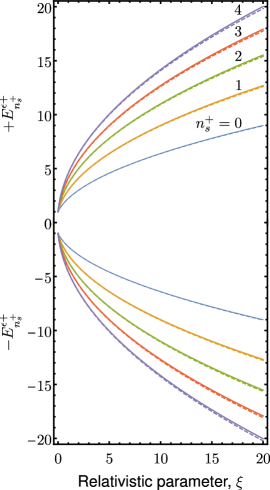
Figure 1: (Color online) JC (solid lines) and the $\kappa$-JC (dashed lines) eigenenergies $E_{n_{s}}^{\epsilon+}$ as a function of the relativistic parameter $\xi$, in units such as $\hbar=m=c=1$, for $n_{s}^{+}=0,\ldots,4$. The value used for the dimensionless deformation parameter is $\epsilon=5\times 10^{-4}$.

IV Symmetries and the non-Hermiticity of the $\kappa$-JC and $\kappa$-AJC models

As we stated above, $H_{\epsilon}^{\pm}$ is non-Hermitian and it leads to a non-unitary evolution. In fact, the $\kappa$-deformed Hamiltonian is not even $\mathcal{PT}$-symmetric, but it is quasi-Hermitian. We can check this by first looking at the effects of parity and time reversal symmetry operations on $a$’s and $\sigma$’s operators [48]:

$$\mathcal{P}a_{s}^{\pm}\mathcal{P}^{-1} =a_{-s}^{\pm}, \mathcal{P}\sigma_{z}\mathcal{P}^{-1} =\sigma_{z}, \mathcal{P}\sigma^{\pm}\mathcal{P}^{-1} =\sigma^{\pm},$$

$$\mathcal{T}a_{s}^{\pm}\mathcal{T}^{-1} =-a_{s}^{\pm}, \mathcal{T}\sigma_{z}\mathcal{T}^{-1} =-\sigma_{z}, \mathcal{T}\sigma^{\pm}\mathcal{T}^{-1} =\sigma^{\mp}.$$

Through this, one notes that the deformed Hamiltonian in Eq. (III) is not $\mathcal{PT}$-symmetric since

$$\mathcal{PT}H_{\epsilon}^{\pm}(\mathcal{PT})^{-1}={} \hbar\left(ga^{+}_{\pm s}\sigma^{\mp}\mu_{\epsilon}^{\mp}+g^{*}a^{-}_{\pm s}\sigma^{\pm}\mu_{\epsilon}^{\pm}\right)-\delta_{\epsilon}^{\pm}\sigma_{z}$$

$$-2mc^{2}\epsilon\xi(2N_{\pm s}+1)\mathbbm{1}$$

$$\neq{} H_{\epsilon}^{\pm}.$$ (26)

However, the Hamiltonian is invariant under the transformation $\mathcal{P}\sigma_{z}$, so that

$$\mathcal{P}\sigma_{z}H_{\epsilon}^{\pm}(\mathcal{P}\sigma_{z})^{-1}=H_{\epsilon}^{\pm}.$$ (27)

This symmetry was also observed in a similar system in Ref. [49]. Another interesting transformation is given by

$$\mathcal{T}\sigma_{x}H_{\epsilon}^{\pm}{(\mathcal{T}\sigma_{x})}^{-1}={} \hbar\left(ga^{+}_{\mp s}\sigma^{\mp}\mu_{\epsilon}^{\mp}+g^{*}a^{-}_{\mp s}\sigma^{\pm}\mu_{\epsilon}^{\pm}\right)+\delta_{\epsilon}^{\pm}\sigma_{z}$$

$$-2mc^{2}\epsilon\xi(2N_{\mp s}+1)\mathbbm{1},$$ (28)

which leads to the original Hamiltonian but with the chirality changed, $s\rightarrow-s$. Although the Hamiltonian is not $\mathcal{PT}$-symmetric, it is quasi-Hermitian since its eigenvalues are real [7]. Therefore, the Hamiltonian satisfies a quasi-Hermiticity relation

$${H_{\epsilon}^{\pm}}^{\dagger}=\eta_{\pm}H_{\epsilon}^{\pm}\eta_{\pm}^{-1},$$ (29)

for some positive-defined operator $\eta_{\pm}$ , the so-called metric operator, which defines the inner-product

$$\langle\cdot,\cdot\rangle_{\eta_{\pm}}=\langle\cdot,\eta_{\pm}\cdot\rangle,$$ (30)

with respect to which the Hamiltonian is said to be Hermitian since

$$\langle\phi,H_{\epsilon}^{\pm}\psi\rangle_{\eta_{\pm}}={} \langle\phi|\eta_{\pm}H_{\epsilon}^{\pm}|\psi\rangle$$

$$={} \langle\phi|{H_{\epsilon}^{\pm}}^{\dagger}\eta_{\pm}|\psi\rangle$$

$$={} \langle{H_{\epsilon}^{\pm}}\phi,\psi\rangle_{\eta_{\pm}},$$ (31)

for all $\phi$ and $\psi$ in the domain of $H_{\epsilon}^{\pm}$. Thus, decomposing the metric operator as $\eta_{\pm}={\rho_{\pm}}^{\dagger}\rho_{\pm}$, Eq. (29) allows us to define a Hermitian counterpart associated with the non-Hermitian one,

$$h_{\epsilon}^{\pm}=\rho_{\pm}H_{\epsilon}^{\pm}{\rho_{\pm}}^{\dagger},$$ (32)

in such a way that $h_{\epsilon}^{\pm}={h_{\epsilon}^{\pm}}^{\dagger}$. The expected values in both representations are the same

$$\langle H_{\epsilon}^{\pm}\rangle_{\eta_{\pm},\Phi}={} \langle\Phi|\eta_{\pm}H_{\epsilon}^{\pm}|\Phi\rangle$$

$$={} \langle\Phi|{\rho_{\pm}}^{\dagger}h_{\epsilon}^{\pm}\rho_{\pm}|\Phi\rangle$$

$$={} \langle\Psi|h_{\epsilon}^{\pm}|\Psi\rangle$$

$$={} \langle h_{\epsilon}^{\pm}\rangle_{\Psi},$$ (33)

with $|\Psi\rangle=\rho_{\pm}|\Phi\rangle$.

V System dynamics

Until now we have worked with both $\kappa$-JC and $\kappa$-AJC systems simultaneously. For the sake of clarity, in what follows we focus our discussion on the $\kappa$-JC Hamiltonian, $H^{s}_{\kappa\text{--JC}}=H_{\epsilon}^{+}$. At the end we comment briefly on how to obtain the results for the $\kappa$-AJC Hamiltonian, $H^{-s}_{\kappa\text{--AJC}}=H_{\epsilon}^{-}$. Thus, to simplify the notation, we drop the $+$ signal in our equations. To obtain the Hermitian operator associated with $H_{\kappa\text{--JC}}^{s}$, a suitable similarity transformation is given by the operator

$$\rho=e^{\epsilon a^{-}_{s}a^{-}_{s}-\epsilon a^{+}_{s}a^{+}_{s}+\epsilon a^{+}_{s}a^{-}_{s}},$$ (34)

satisfying $\rho^{\dagger}\rho=\eta$. Note that this operator is a function of creation and annihilation operators with same chiralities and reduces to the identity operator for $\epsilon=0$. Thus, the Hermitian operator can be obtained from the similarity transformation

$$h_{\kappa\text{--JC}}^{s}=\rho H_{\kappa\text{--JC}}^{s}\rho^{-1},$$ (35)

with $\rho^{\dagger}\rho=\eta$. The result seems to be

$$h^{s}_{\kappa\text{--JC}}={} \hbar(g\sigma^{-}a_{s}^{+}+g^{*}\sigma^{+}a_{s}^{-})+(1-2\epsilon\xi)\delta\sigma_{z}$$

$$+\epsilon\hbar(g\sigma^{-}a_{s}^{-}+g^{*}\sigma^{+}a_{s}^{+})$$

$$-2mc^{2}\epsilon\xi(2N_{s}+1)\mathbbm{1}.$$ (36)

The spectrum of the Hermitian operator $h_{\kappa\text{--JC}}^{s}$ is given by (25) as it shares the spectrum with the non-Hermitian operator $H_{\kappa\text{--JC}}^{s}$. To find the associated deformed energy eigenstates for the positive and negative deformed energy eigenvalues of $h_{\kappa\text{JC}}^{s}$, we first solve the eigenvalue equation for the non-Hermitian operator, $H_{\kappa\text{--JC}}^{s}\ket{E_{n_{s}}^{\epsilon}}=E_{n_{s}}^{\epsilon}\ket{E_{n_{s}}^{\epsilon}}$, then apply the transformation $\rho$. In this manner, using the Pauli spinors $\ket{{\uparrow}}=(1,0)^{\dagger}$ and $\ket{{\downarrow}}=(0,1)^{\dagger}$, the deformed energy eigenstates of $H_{\kappa\text{--JC}}^{s}$ can be written as

$$\ket{\pm E_{n_{s}}^{\epsilon}}={} \sqrt{\frac{E_{n_{s}}\pm mc^{2}}{2E_{n_{s}}}}\ket{n_{s}}\ket{{\uparrow}}$$

$$\pm i\sqrt{\frac{E_{n_{s}}\mp mc^{2}}{2E_{n_{s}}}}(1-\epsilon)\ket{n_{s}+1}\ket{{\downarrow}},$$ (37)

and by applying the transformation $\rho$, we obtain

$$\ket{+\bar{E}_{n_{s}}^{\epsilon}}={} \rho\ket{+E_{n_{s}}^{\epsilon}}$$

$$={} \alpha_{n_{s}}\ket{n_{s}}\ket{{\uparrow}}+i\beta_{n_{s}}\ket{n_{s}+1}\ket{{\downarrow}}$$

$$+\epsilon\alpha_{n_{s}}\left(c_{n_{s}}\ket{n_{s}-2}\ket{{\uparrow}}-c_{n_{s}+2}\ket{n_{s}+2}\ket{{\uparrow}}\right)$$

$$+i\epsilon\beta_{n_{s}}\left(c_{n_{s}+1}\ket{n_{s}-1}\ket{{\downarrow}}-c_{n_{s}+3}\ket{n_{s}+3}\ket{{\downarrow}}\right),$$ (38)

and

$$\ket{-\bar{E}_{n_{s}}^{\epsilon}}={} \rho\ket{-E_{n_{s}}^{\epsilon}}$$

$$={} \beta_{n_{s}}\ket{n_{s}}\ket{{\uparrow}}-i\alpha_{n_{s}}\ket{n_{s}+1}\ket{{\downarrow}}$$

$$+\epsilon\beta_{n_{s}}\left(c_{n_{s}}\ket{n_{s}-2}\ket{{\uparrow}}-c_{n_{s}+2}\ket{n_{s}+2}\ket{{\uparrow}}\right)$$

$$-i\epsilon\alpha_{n_{s}}\left(c_{n_{s}}\ket{n_{s}-1}\ket{{\downarrow}}-c_{n_{s}+3}\ket{n_{s}+3}\ket{{\downarrow}}\right),$$ (39)

with

$$\alpha_{n_{s}}=\sqrt{\dfrac{E_{n_{s}}+mc^{2}}{2E_{n_{s}}}},\qquad\beta_{n_{s}}=\sqrt{\dfrac{E_{n_{s}}-mc^{2}}{2E_{n_{s}}}},$$ (40)

and $c_{n_{s}}=\sqrt{n_{s}(n_{s}-1)}$. Note that the eigenstates in (V) and (V) are normalized up to first order in $\epsilon$ and, as observed in [42], these eigenstates show that the spin and angular momentum are entangled. Moreover, the presence of deformation gives rise to new entangled states. Equations (V) and (V) allow us to write an initial state $\ket{\Psi_{n_{s}}(0)}=\ket{n_{s}}\ket{{\uparrow}}$ in terms of the positive- and negative-energy eigenstates, namely

$$\ket{\Psi_{n_{s}}(0)}={} \alpha_{n_{s}}\ket{+\bar{E}_{n_{s}}^{\epsilon}}+\beta_{n_{s}}\ket{-\bar{E}_{n_{s}}^{\epsilon}}$$

$$-\epsilon c_{n_{s}}\left(\alpha_{n_{s}-2}\ket{+\bar{E}_{n_{s}-2}^{\epsilon}}+\beta_{n_{s}-2}\ket{-\bar{E}_{n_{s}-2}^{\epsilon}}\right)$$

$$+\epsilon c_{n_{s}+2}\left(\alpha_{n_{s}+2}\ket{+\bar{E}_{n_{s}+2}^{\epsilon}}+\beta_{n_{s}+2}\ket{-\bar{E}_{n_{s}+2}^{\epsilon}}\right).$$ (41)

This superposition of the positive- and negative-energy eigenstates is a signature of the Zitterbewegung, which here is encoded in the spin degree of freedom, and can be associated to Rabi oscillations due to the interference of these eigenstates [42]. The Zitterbewegung is a relativistic quantum effect generally understood as a trembling motion of relativistic particles [51], difficult to be measured, but can be simulated experimentally in one dimension [52]. We observe again that the deformation introduces more eigenstates in the superposition and for $\epsilon=0$ our results immediately reduce to the ones in Ref. [42].

Now that we have a Hermitian operator and its eigenstates, we can proceed to study the system dynamics. Thus starting with (V), it leads to a state at time $t$ given by

$$\ket{\Psi_{n_{s}}(t)}={} \alpha_{n_{s}}\ket{+\bar{E}_{n_{s}}^{\epsilon}}e^{-i\omega^{\epsilon+}_{n_{s}}t}+\beta_{n_{s}}\ket{-\bar{E}_{n_{s}}^{\epsilon}}e^{-i\omega^{\epsilon-}_{n_{s}}t}$$

$$-\epsilon c_{n_{s}}\alpha_{n_{s}-2}\ket{+\bar{E}_{n_{s}-2}^{\epsilon}}e^{-i\omega^{\epsilon+}_{n_{s}-2}t}-\epsilon c_{n_{s}}\beta_{n_{s}-2}\ket{-\bar{E}_{n_{s}-2}^{\epsilon}}e^{-i\omega^{\epsilon-}_{n_{s}-2}t}$$

$$+\epsilon c_{n_{s}+2}\alpha_{n_{s}+2}\ket{+\bar{E}_{n_{s}+2}^{\epsilon}}e^{-i\omega^{\epsilon+}_{n_{s}+2}t}+\epsilon c_{n_{s}+2}\beta_{n_{s}+2}\ket{-\bar{E}_{n_{s}+2}^{\epsilon}}e^{-i\omega^{\epsilon-}_{n_{s}+2}t},$$ (42)

where

$$\omega^{\epsilon\pm}_{n_{s}}=\pm\omega_{n_{s}}-\phi_{n_{s}}^{\epsilon},$$ (43)

is the $\kappa$-deformed Zitterbewegung frequency, with $\omega_{n_{s}}=E^{+}_{n_{s}}/\hbar$, and $\phi_{n_{s}}^{\epsilon}=4m^{2}c^{4}\epsilon\xi(n_{s}+1)/\hbar$. Now, writing the evolved state in the language of Pauli spinors, we have

$$\ket{\Psi_{n_{s}}(t)}={} e^{i\phi_{n_{s}}^{\epsilon}t}\left(f_{n_{s}}(t)\ket{n_{s}}\ket{{\uparrow}}+g_{n_{s}}(t)\ket{n_{s}+1}\ket{{\downarrow}}\right)$$

$$+\epsilon e^{i\phi_{n_{s}}^{\epsilon}t}\left[c_{n_{s}}f_{n_{s}}(t)\ket{n_{s}-2}\ket{{\uparrow}}+c_{n_{s}+1}g_{n_{s}}(t)\ket{n_{s}-1}\ket{{\downarrow}}\right]$$

$$-\epsilon e^{i\phi_{n_{s}}^{\epsilon}t}\left(c_{n_{s}+2}f_{n_{s}}(t)\ket{n_{s}+2}\ket{{\uparrow}}-c_{n_{s}+3}g_{n_{s}}(t)\ket{n_{s}+3}\ket{{\downarrow}}\right)$$

$$-\epsilon c_{n_{s}}e^{i\phi_{n_{s}-2}^{\epsilon}t}\left(f_{n_{s}-2}(t)\ket{n_{s}-2}\ket{{\uparrow}}+g_{n_{s}-2}(t)\ket{n_{s}-1}\ket{{\downarrow}}\right)$$

$$+\epsilon c_{n_{s}+2}e^{i\phi_{n_{s}+2}^{\epsilon}t}\left(f_{n_{s}+2}(t)\ket{n_{s}+2}\ket{{\uparrow}}+g_{n_{s}+2}(t)\ket{n_{s}+3}\ket{{\downarrow}}\right),$$ (44)

where

$$f_{n_{s}}(t)=\cos(\omega_{n_{s}}t)-\frac{i\sin(\omega_{n_{s}}t)}{\sqrt{1+4\xi(n_{s}+1)}},$$ (45)

and

$$g_{n_{s}}(t)=2\sin(\omega_{n_{s}}t)\alpha_{n_{s}}\beta_{n_{s}},$$ (46)

with $|f_{n_{s}}(t)|^{2}+|g_{n_{s}}(t)|^{2}=1$.

We can appreciate the modifications caused by the $\kappa$-deformation by evaluating the expectation values of the $z$ component of the spin, orbital and total angular momentum observables, which are defined by

$$S_{z}=\frac{\hbar}{2}\sigma_{z},\quad L_{z}=\hbar(N_{s}-N_{-s}),\quad J_{z}=L_{z}+S_{z},$$ (47)

respectively. Surprisingly, even though the $\kappa$-deformation modifies the energy eigenvalues, gives rise to new entangled states with different quantum numbers, and modifies the Zitterbewegung frequency, there is no first-order correction on the expectation values of the $\kappa$-JC. This kind of result was already observed in the $\kappa$-Dirac-Coulomb problem [18], where the first-order correction on this system is identically zero.

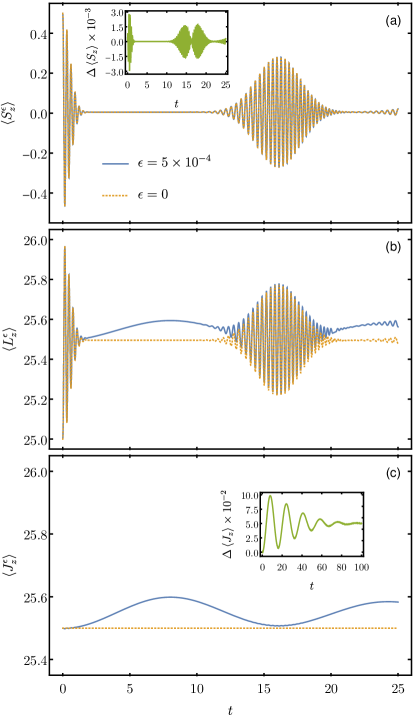
Figure 2: (Color online) Behavior of the expectation values (a) $\expectationvalue{S_{z}^{\epsilon}}$, (b) $\expectationvalue{L_{z}^{\epsilon}}$, and (c) $\expectationvalue{J_{z}^{\epsilon}}$ as a function of time for a system with mean photon number $\expectationvalue{n_{s}}=25$ for $\epsilon=5\times 10^{-4}$ (blue solid line) and $\epsilon=0$ (orange dotted line) using units such as $m=\hbar=\omega=c=1$. In (a), the two curves are superposed and the inset shows the difference between them. In (c), the inset shows the asymptotic behavior of the $\Delta\expectationvalue{J_{z}^{\epsilon}}$.

On the other hand, we can observe first-order effects of the $\kappa$-deformation on the scenario of collapsed and revivals of the atomic population in the $\kappa$-JC model by employing an initial coherent state. Thus, considering the initial state as $\ket{\Psi_{n_{s}}(0)}=\ket{\alpha}\ket{{\uparrow}}$, with

$$\ket{\alpha}=e^{-\frac{|\alpha|^{2}}{2}}\sum_{n_{s}=0}^{\infty}\frac{\alpha^{n_{s}}}{\sqrt{n_{s}!}}\ket{n_{s}},$$ (48)

the $\kappa$-deformed expectation values are given by

$$\expectationvalue{S_{z}^{\epsilon}}={} \frac{\hbar}{2}-\hbar\sum_{n_{s}=0}^{\infty}\frac{\expectationvalue{n_{s}}^{n_{s}}e^{-\expectationvalue{n_{s}}}}{n_{s}!}\mathcal{S}_{n_{s}}(t)$$

$$+\hbar\epsilon\sum_{n_{s}=0}^{\infty}\frac{\expectationvalue{n_{s}}^{n_{s}+1}e^{-\expectationvalue{n_{s}}}}{n!}[\mathcal{S}_{n_{s}}(t)-\mathcal{S}_{n_{s}+2}(t)],$$ (49)

$$\expectationvalue{L_{z}^{\epsilon}}={} \hbar\expectationvalue{n_{s}}+\hbar\sum_{n_{s}=0}^{\infty}\frac{\expectationvalue{n_{s}}^{n_{s}}e^{-\expectationvalue{n_{s}}}}{n_{s}!}\mathcal{S}_{n_{s}}(t)$$

$$-\hbar\epsilon\sum_{n_{s}=0}^{\infty}\frac{\expectationvalue{n_{s}}^{n_{s}+1}e^{-\expectationvalue{n_{s}}}}{n!}[\mathcal{S}_{n_{s}}(t)-\mathcal{S}_{n_{s}+2}(t)]$$

$$+\hbar\epsilon\sum_{n_{s}=0}^{\infty}\frac{\expectationvalue{n_{s}}^{n_{s}+1}e^{-\expectationvalue{n_{s}}}}{n!}\mathcal{L}_{n_{s}}^{\epsilon}(t),$$ (50)

and

$$\expectationvalue{J_{z}^{\epsilon}}={} \hbar\left[\expectationvalue{n_{s}}+\frac{1}{2}\right]+\hbar\epsilon\sum_{n_{s}=0}^{\infty}\frac{\expectationvalue{n_{s}}^{n_{s}+1}e^{-\expectationvalue{n_{s}}}}{n!}\mathcal{L}_{n_{s}}^{\epsilon}(t),$$ (51)

where $\expectationvalue{n_{s}}=|\alpha|^{2}$,

$$\mathcal{S}_{n_{s}}(t)={} \frac{4\xi(n_{s}+1)}{[1+4\xi(n_{s}+1)]}\sin^{2}{(\omega_{n_{s}}t)},$$ (52)

$$\mathcal{L}_{n_{s}}^{\epsilon}(t)={} \frac{4c_{n_{s}+2}}{\sqrt{(n_{s}+2)!}}-\frac{2c_{n_{s}+2}}{\sqrt{(n_{s}+2)!}}w_{n_{s}}(t)\cos(\Phi^{\epsilon}t)$$

$$-\frac{2c_{n_{s}+2}}{\sqrt{(n_{s}+2)!}}s_{n_{s}}(t)\sin(\Phi^{\epsilon}t)$$

$$-\frac{2c_{n_{s}+3}}{\sqrt{(n_{s}+2)!}}p_{n_{s}}(t)\cos(\Phi^{\epsilon}t),$$ (53)

with

$$\Phi^{\epsilon}=\phi_{n_{s}}^{\epsilon}-\phi_{n_{s}+2}^{\epsilon}=-8m^{2}c^{4}\xi\epsilon,$$ (54)

$$w_{n_{s}}(t)={} 2\cos(\omega_{n_{s}}t)\cos(\omega_{n_{s}+2}t)$$

$$+\frac{2\sin(\omega_{n_{s}}t)\sin(\omega_{n_{s}+2}t)}{\sqrt{[1+4\xi(n_{s}+1)][1+4\xi(n_{s}+3)]}},$$ (55)

$$s_{n_{s}}(t)={} \frac{2\cos(\omega_{n_{s}+2}t)\sin(\omega_{n_{s}}t)}{\sqrt{1+4\xi(n_{s}+1)}}$$

$$-\frac{2\cos(\omega_{n_{s}}t)\sin(\omega_{n_{s}+2}t)}{\sqrt{1+4\xi(n_{s}+3)}},$$ (56)

and

$$p_{n_{s}}(t)=2\alpha_{n_{s}}\alpha_{n_{s}+2}\sin(\omega_{n_{s}}t)\sin(\omega_{n_{s}+2}t).$$ (57)

We can observe that the deformation modifies all the expectation values. To help us analyze the effects of the deformation on the expectation values, let us define

$$\Delta\expectationvalue{O}=\expectationvalue{O^{\epsilon}}-\expectationvalue{O},$$ (58)

as the difference between the $\kappa$-deformed expectation value of the observable $O$ and the usual (undeformed) one. Figure 2 shows the results for the expectation values as a function of time $t$ for a system with mean photon number $\expectationvalue{n_{s}}=25$, using units such as $m=\hbar=\omega=c=1$ and $\epsilon=5\times 10^{-4}$ (blue solid lines) and for $\epsilon=0$ (orange dotted lines). In Fig. 2(a) we show $\expectationvalue{S_{z}^{\epsilon}}$ and it shows the well-known initial collapse followed by the revival of the spin inversion. The inset shows $\Delta\expectationvalue{S_{z}}$ and we observe that the expectation value is slightly modified by the deformation. On the other hand, in Fig. 2(b) we show the $\expectationvalue{L_{z}^{\epsilon}}$ and we can also observe collapse and revival, but now the orbital angular momentum is noticeably more affected by the deformation than the spin angular momentum. As a result, we observe that $\expectationvalue{J_{z}^{\epsilon}}$ is not constant of motion anymore when the deformation is present, as we can see in Fig. 2(c). So, the $\kappa$-deformed expectation value of the $z$ component of the total angular momentum is not a conserved quantity. This result can be understood by noting that $J_{z}$ fails to commute with $h_{\kappa\text{--JC}}^{s}$,

$$[h_{\kappa\text{--JC}}^{s},J_{z}]=4\epsilon\hbar g(\sigma^{-}\hat{a}^{-}_{s}+\sigma^{+}\hat{a}^{+}_{s}),$$ (59)

and this failure is a direct consequence of the deformation. We can also observe that deformation displaces the expectation value of the $J_{z}$ [see the inset in Fig 2(c)] and for large values of $t$ it converges to a fixed amount, $\Delta\expectationvalue{J_{z}}|_{t\to\infty}\sim 5\times 10^{-2}$. It is easy to see that for $\epsilon=0$, $J_{z}$ commutes with the Hamiltonian and we recover all the results of the usual JC system, as it should be.

Finally, we end up saying that for the $\kappa$-AJC Hamiltonian, we observe that a suitable similarity transformation is

$$\rho=e^{\epsilon a^{-}_{s}a^{-}_{s}-\epsilon a^{+}_{s}a^{+}_{s}-\epsilon a^{+}_{s}a^{-}_{s}},$$ (60)

in which, in comparison with the map for the $\kappa$-JC in Eq. (34), the last term has a sign reversal, and leads us to the following Hermitian $\kappa$-AJC Hamiltonian

$$h_{\kappa\text{--AJC}}^{-s}={} \rho H_{\kappa\text{--AJC}}^{-s}\rho^{-1}$$

$$={} \hbar(g\sigma^{+}a_{-s}^{+}+g^{*}\sigma^{-}a_{-s}^{-})+(1+2\epsilon\xi)\delta\sigma_{z}$$

$$+\epsilon\hbar(g\sigma^{+}a_{-s}^{-}+g^{*}\sigma^{-}a_{-s}^{+})$$

$$-2mc^{2}\epsilon\xi(2N_{-s}+1)\mathbbm{1}.$$ (61)

Thus it is straightforward to show that similar results can be obtained for the $\kappa$-AJC system by using the Hermitian Hamiltonian $h_{\kappa\text{--AJC}}^{-s}$.

VI Conclusion

In conclusion, we have revisited the Dirac oscillator in (2+1) dimensions and its mapping onto the JC and AJC models. The mapping is now transparent as we have made the connection between the non-minimal coupling signal $+$ ($-$) of the Dirac oscillator Hamiltonian and the JC (AJC) model. We have also introduced the parameter $s=\pm 1$ to characterize the two possible chiralities, allowing one to discuss them simultaneously. By considering the (2+1) Dirac oscillator in the context of the $\kappa$-deformed algebra and using the above mapping, we have proposed the $\kappa$-JC and the $\kappa$-AJC models. We have shown that the $\kappa$-deformation leads naturally to a non-Hermitian Hamiltonian, something that leads to a non-unitary time evolution. Moreover, the $\kappa$-(A)JC Hamiltonian is not even $\mathcal{PT}$-symmetric, but is quasi-Hermitian as it possesses a real spectrum, and by employing the theory of quasi-Hermitian Hamiltonians, we have found its Hermitian counterpart, allowing us to study the dynamics of the $\kappa$-deformed system. Although the displacement was caused by the deformation on the eigenenergies and, consequently, on the Zitterbewegung frequencies, we have observed no first-order effects on the expectation values of $S_{z}$, $L_{z}$, and $J_{z}$, when considering an initial state such as $\ket{\Psi_{n_{s}}(0)}=\ket{n_{s}}\ket{\uparrow}$. On the other hand, when considering a coherent initial state, we have observed modifications on the well-known collapse and revival behavior, as well as on the above expectation values. Especially, we have observed that the expectation value of the total angular momentum in the $z$ direction, $J_{z}$, is not a constant of motion anymore as a direct consequence of the $\kappa$-deformation.

We comment that the mapping between quantum optical and relativistic quantum systems [53] led to a great breakthrough in quantum simulation experiments of relativistic quantum effects [52] since direct measurements of relativistic quantum phenomena are not easy to do. Significant examples of relativistic quantum effects simulated through optical setups are the experimental simulation of the Zitterbewegung effect in trapped ions [54] and others [55, 56]. As shown in [42], the dynamics of the 2D Dirac oscillator can be implemented in a single trapped ion inside a Paul trap, and given the fact these systems allow a vast coherent control of ionic internal and external degrees of freedom [57], and the ability to tune experimental parameters that could also introduce certain modifications that would entail novel phenomena, our work suggests that some future experiment might be able to detect the effects of the $\kappa$-deformation presented here.

References

- Bender and Boettcher [1998] C. M. Bender and S. Boettcher, Real spectra in non-hermitian hamiltonians HavingPTSymmetry, Phys. Rev. Lett. 80, 5243 (1998).
- Bender [2005] C. M. Bender, Introduction to -symmetric quantum theory, Contemp. Phys. 46, 277 (2005).
- Bender [2007] C. M. Bender, Making sense of non-hermitian hamiltonians, Rep. Progr. Phys. 70, 947 (2007).
- Novitsky et al. [2018] D. V. Novitsky, A. Karabchevsky, A. V. Lavrinenko, A. S. Shalin, and A. V. Novitsky, PT symmetry breaking in multilayers with resonant loss and gain locks light propagation direction, Phys. Rev. B 98, 125102 (2018).
- Klauck et al. [2019] F. Klauck, L. Teuber, M. Ornigotti, M. Heinrich, S. Scheel, and A. Szameit, Observation of PT-symmetric quantum interference, Nat. Photonics 13, 883 (2019).
- Scholtz et al. [1992] F. Scholtz, H. Geyer, and F. Hahne, Quasi-hermitian operators in quantum mechanics and the variational principle, Ann. Phys. (NY) 213, 74 (1992).
- Croke [2015] S. Croke, PT-symmetric hamiltonians and their application in quantum information, Phys. Rev. A 91, 052113 (2015).
- Fring and Moussa [2016] A. Fring and M. H. Y. Moussa, Unitary quantum evolution for time-dependent quasi-hermitian systems with nonobservable hamiltonians, Phys. Rev. A 93, 042114 (2016).
- Dyson [1956] F. J. Dyson, Thermodynamic behavior of an ideal ferromagnet, Phys. Rev. 102, 1230 (1956).
- Lukierski et al. [1991] J. Lukierski, H. Ruegg, A. Nowicki, and V. N. Tolstoy, q-deformation of poincaré algebra, Phys. Lett. B 264, 331 (1991).
- Lukierski et al. [1992] J. Lukierski, A. Nowicki, and H. Ruegg, New quantum poincaré algebra and -deformed field theory, Phys. Lett. B 293, 344 (1992).
- Lukierski and Ruegg [1994] J. Lukierski and H. Ruegg, Quantum -poincaré in any dimension, Phys. Lett. B 329, 189 (1994).
- Majid and Ruegg [1994] S. Majid and H. Ruegg, Bicrossproduct structure of -poincare group and non-commutative geometry, Phys. Lett. B 334, 348 (1994).
- Kovacević et al. [2012] D. Kovacević, S. Meljanac, A. Pachoł, and R. Štrajn, Generalized poincaré algebras, hopf algebras and -minkowski spacetime, Phys. Lett. B 711, 122 (2012).
- Liu et al. [2018] X. Liu, Z. Tian, J. Wang, and J. Jing, Relativistic motion enhanced quantum estimation of -deformation of spacetime, Eur. Phys. J. C 78, 665 (2018).
- Kowalski-Glikman [2017] J. Kowalski-Glikman, A short introduction to -deformation, Int. J. Modern Phys. A 32, 1730026 (2017).
- Nowicki et al. [1993] A. Nowicki, E. Sorace, and M. Tarlini, The quantum deformed dirac equation from the -poincaré algebra, Phys. Lett. B 302, 419 (1993).
- Biedenharn et al. [1993] L. Biedenharn, B. Mueller, and M. Tarlini, The dirac-coulomb problem for the -poincaré quantum group, Phys. Lett. B 318, 613 (1993).
- Agostini et al. [2004] A. Agostini, G. Amelino-Camelia, and M. Arzano, Dirac spinors for doubly special relativity and -minkowski noncommutative spacetime, Class. Quantum Grav. 21, 2179 (2004).
- Aloisio et al. [2004] R. Aloisio, A. Galante, A. F. Grillo, F. Méndez, J. M. Carmona, and J. L. Cortés, Particle and antiparticle sectors in DSr1 and -minkowski space-time, J. High Energy Phys. 2004 (05), 028.
- Arzano and Marcianò [2007] M. Arzano and A. Marcianò, Fock space, quantum fields, and -poincaré symmetries, Phys. Rev. D 76, 125005 (2007).
- Andrade and Silva [2013] F. M. Andrade and E. O. Silva, Effects of quantum deformation on the spin-1/2 Aharonov-bohm problem, Phys. Lett. B 719, 467 (2013).
- Roy and Roychoudhury [1995] P. Roy and R. Roychoudhury, Aharonov-bohm interaction for a deformed non-relativistic spin 1/2 particle, Phys. Lett. B 359, 339 (1995).
- Roy and Roychoudhury [1994] P. Roy and R. Roychoudhury, A note on the -deformed landau problem, Phys. Lett. B 339, 87 (1994).
- Andrade et al. [2016] F. M. Andrade, E. O. Silva, D. Assafrão, and C. Filgueiras, Effects of quantum deformation on the integer quantum hall effect, Europhys. Lett. 116, 31002 (2016).
- Andrade et al. [2014] F. M. Andrade, E. O. Silva, M. M. Ferreira Jr., and E. C. Rodrigues, On the -dirac oscillator revisited, Phys. Lett. B 731, 327 (2014).
- Andrade and Silva [2014a] F. M. Andrade and E. O. Silva, The 2D -dirac oscillator, Phys. Lett. B 738, 44 (2014a).
- Lee and Chan [2014] T. E. Lee and C.-K. Chan, Heralded magnetism in non-hermitian atomic systems, Phys. Rev. X 4, 041001 (2014).
- Naghiloo et al. [2019] M. Naghiloo, M. Abbasi, Y. N. Joglekar, and K. W. Murch, Quantum state tomography across the exceptional point in a single dissipative qubit, Nat. Phys. 15, 1232 (2019).
- Wang et al. [2021] K. Wang, A. Dutt, K. Y. Yang, C. C. Wojcik, J. Vučković, and S. Fan, Generating arbitrary topological windings of a non-hermitian band, Science 371, 1240 (2021).
- Makris et al. [2008] K. G. Makris, R. El-Ganainy, D. N. Christodoulides, and Z. H. Musslimani, Beam dynamics inPTSymmetric optical lattices, Phys. Rev. Lett. 100, 103904 (2008).
- Itô et al. [1967] D. Itô, K. Mori, and E. Carriere, An example of dynamical systems with linear trajectory, Nuovo Cimento A 51, 1119 (1967).
- Moshinsky and Szczepaniak [1989] M. Moshinsky and A. Szczepaniak, The dirac oscillator, J. Phys. A: Math. Gen. 22, L817 (1989).
- Martinez-y Romero et al. [1995] R. P. Martinez-y Romero, H. N. Nunez-Yepez, and A. L. Salas-Brito, Relativistic quantum mechanics of a dirac oscillator, Eur. J. Phys. 16, 135 (1995).
- Franco-Villafañe et al. [2013] J. A. Franco-Villafañe, E. Sadurní, S. Barkhofen, U. Kuhl, F. Mortessagne, and T. H. Seligman, First experimental realization of the dirac oscillator, Phys. Rev. Lett. 111, 170405 (2013).
- Zhang et al. [2018] K. Zhang, L. Zhou, P. Meystre, and W. Zhang, Relativistic measurement backaction in the quantum dirac oscillator, Phys. Rev. Lett. 121, 110401 (2018).
- Strange [1998] P. Strange, Relativistic Quantum Mechanics (Cambridge University Press, 1998).
- Moshinsky and Smirnov [1996] M. Moshinsky and Y. Smirnov, The Harmonic Oscillator in Modern Physics, Contemporary concepts in physics (Harwood Academic Publishers, 1996).
- Sadurni [2011] E. Sadurni, The dirac-moshinsky oscillator: theory and applications, AIP Conf. Proc. 1334, 249 (2011), 1101.3011 .
- Andrade and Silva [2014b] F. M. Andrade and E. O. Silva, Remarks on the dirac oscillator in (2 + 1) dimensions, Europhys. Lett. 108, 30003 (2014b).
- Bermudez et al. [2008] A. Bermudez, M. A. Martin-Delgado, and A. Luis, Nonrelativistic limit in the (2+1) dirac oscillator: A ramsey-interferometry effect, Phys. Rev. A 77, 033832 (2008).
- Bermudez et al. [2007] A. Bermudez, M. A. Martin-Delgado, and E. Solano, Exact mapping of the 2+1 dirac oscillator onto the jaynes-cummings model: Ion-trap experimental proposal, Phys. Rev. A 76, 041801(R) (2007).
- Villalba [1994] V. M. Villalba, Exact solution of the two-dimensional dirac oscillator, Phys. Rev. A 49, 586 (1994).
- Hagen [1990] C. R. Hagen, Aharonov-bohm scattering of particles with spin, Phys. Rev. Lett. 64, 503 (1990).
- Majari et al. [2017] P. Majari, A. Luis, and M. R. Setare, Mapping of the 2 + 1 q-deformed dirac oscillator onto the q-deformed jaynes-cummings model, Europhys. Lett. 120, 44002 (2017).
- Setare and Majari [2017] M. R. Setare and P. Majari, (2+1) -dimensional f-deformed dirac oscillator as f-deformed AJC model, Eur. Phys. J. Plus 132, 458 (2017).
- dos Santos et al. [2019] J. F. G. dos Santos, F. S. Luiz, O. S. Duarte, and M. H. Y. Moussa, Non-hermitian noncommutative quantum mechanics, Eur. Phys. J. Plus 134, 332 (2019).
- Sakurai and Napolitano [2011] J. J. Sakurai and J. Napolitano, Modern Quantum Mechanics, 2nd ed. (Addison-Wesley, 2011).
- Mandal [2005] B. P. Mandal, Pseudo-hermitian interaction between an oscillator and a spin-1/2 particle in the external magnetic field, Modern Phys. Lett. A 20, 655 (2005).
- Note [1] In order to restrict to theories with positive-definite norm.
- Greiner [2000] W. Greiner, Relativistic Quantum Mechanics. Wave Equations (Springer-Verlag Berlin Heidelberg, 2000).
- Gerritsma et al. [2010] R. Gerritsma, G. Kirchmair, F. Zähringer, E. Solano, R. Blatt, and C. F. Roos, Quantum simulation of the dirac equation, Nature 463, 68 (2010).
- Rozmej and Arvieu [1999] P. Rozmej and R. Arvieu, The dirac oscillator. a relativistic version of the jaynes-cummings model, J. Phys. A: Math. Gen. 32, 5367 (1999).
- Lamata et al. [2007] L. Lamata, J. León, T. Schätz, and E. Solano, Dirac equation and quantum relativistic effects in a single trapped ion, Phys. Rev. Lett. 98, 253005 (2007).
- Schliemann et al. [2005] J. Schliemann, D. Loss, and R. M. Westervelt, Zitterbewegungof electronic wave packets in III-v zinc-blende semiconductor quantum wells, Phys. Rev. Lett. 94, 206801 (2005).
- Garay et al. [2000] L. J. Garay, J. R. Anglin, J. I. Cirac, and P. Zoller, Sonic analog of gravitational black holes in bose-einstein condensates, Phys. Rev. Lett. 85, 4643 (2000).
- Leibfried et al. [2003] D. Leibfried, R. Blatt, C. Monroe, and D. Wineland, Quantum dynamics of single trapped ions, Rev. Mod. Phys. 75, 281 (2003).