Fixed points of nonnegative neural networks

Abstract

We use fixed point theory to analyze nonnegative neural networks, which we define as neural networks that map nonnegative vectors to nonnegative vectors. We first show that nonnegative neural networks with nonnegative weights and biases can be recognized as monotonic and (weakly) scalable functions within the framework of nonlinear Perron-Frobenius theory. This fact enables us to provide conditions for the existence of fixed points of nonnegative neural networks having inputs and outputs of the same dimension, and these conditions are weaker than those recently obtained using arguments in convex analysis. Furthermore, we prove that the shape of the fixed point set of nonnegative neural networks with nonnegative weights and biases is an interval, which under mild conditions degenerates to a point. These results are then used to obtain the existence of fixed points of more general nonnegative neural networks. From a practical perspective, our results contribute to the understanding of the behavior of autoencoders, and the main theoretical results are verified in numerical simulations using the Modified National Institute of Standards and Technology (MNIST) dataset.

Keywords: Nonnegative neural networks, nonlinear Perron-Frobenius theory, monotonic and (weakly) scalable functions, fixed point analysis, convergence analysis.

1 Introduction

Neural networks consist of multiple layers that are able to extract patterns of input signals for decision-making without any human intervention. This fact has profound consequences in a wide range of classification, communications, recognition, image and speech processing tasks, where neural networks set high standards of performance LeCun et al. (2015); Goodfellow et al. (2016); Samek et al. (2021). Neural networks have also recently been introduced as efficient iterative regularization methods in inverse problems, which opens a vista of new applications, especially in medical imaging Adler and Öktem (2017); Benning and Burger (2018); Ongie et al. (2020).

Of our particular interest are nonnegative neural networks, which we define as neural networks that map nonnegative vectors to nonnegative vectors. Nonnegative neural networks have been used in applications such as spectral analysis, and image and text processing, among others – see, for example, Lemme et al. (2012); Nguyen et al. (2013); Chorowski and Zurada (2015); Hosseini-Asl et al. (2015); Zhou et al. (2016); Ali and Yangyu (2017); Ayinde and Zurada (2018); Su et al. (2018); Chen et al. (2019); Yu et al. (2019); Palsson et al. (2019) and references therein. Moreover, restricting the weights to the nonnegative cone has been shown to equip neural networks with the ability of decomposing the input signal into additive sparse components. By doing so, we obtain an understandable hierarchical representation of the input data, which is a feature similar to how the human brain processes sensory inputs Lee and Seung (1999); Shashanka et al. (2008); Lemme et al. (2012); Nguyen et al. (2013); Chorowski and Zurada (2015); Ayinde and Zurada (2018). For example, the main idea of an autoencoder with nonnegative weights is to decompose the input data into additive features in the encoding layer, which are later additively recombined in the decoding layer to reconstruct the original data Lemme et al. (2012); Ayinde and Zurada (2018). In some scenarios, the gains in transparency and interpretation obtained by restricting the weights of the neural network to be nonnegative do not translate into a significant loss of predictive power Nguyen et al. (2013); Chorowski and Zurada (2015).

Neural networks with nonnegative weights have also been increasingly gaining attention in recent years because of the resurgence of analog neural networks, which have been demonstrated to be both readily implementable and more energy efficient than their digital counterparts Kendall et al. (2020); Paliy et al. (2021). In analog networks, the weight parameters are physically encoded in the conductance of programmable resistors. Thus, these analog neural networks are examples of neural networks that are nonnegative because of the laws of physics. Moreover, various approaches can be used to mitigate the loss of predictive power caused by the physical nonnegative constraints Kendall et al. (2020). These results are consistent with those obtained with the digital neural networks in Nguyen et al. (2013); Chorowski and Zurada (2015).

With the objective of improving our understanding of nonnegative neural networks, we shed light on questions related to the existence of fixed points and the shape of the fixed point set of nonnegative neural networks (with matching input and output spaces). To illustrate the importance of fixed point analysis using concrete examples, let us first consider the widely used neural networks known as autoencoders, which can be seen as self-mappings taking the form $T:{}^{k}\to{}^{k}$ with $x\mapsto T_{1}(T_{2}(x))$, where $T_{1}:\mathbb{R}^{k}\to\mathbb{R}^{l}$ with $k>l$ is a mapping (encoder) used to learn compact representations of typical inputs, and $T_{2}:\mathbb{R}^{l}\to\mathbb{R}^{k}$ is a mapping (decoder) used to reconstruct the input from the compact representation obtained with $T_{1}$. From this mathematical perspective, the fixed points of an autoencoder $T$ are exactly the inputs that can be perfectly reconstructed. It is therefore important to determine whether the fixed point set of an autoencoder is nonempty, and if so, how rich this set is (i.e., determine its shape).

As a second example of the importance of fixed point analysis in neural networks, we note that inverse problems are often posed as the minimization of cost functions $f\colon\mathbb{R}^{k}\to\mathbb{R}$ that are solved with fixed point iterations of mappings determined by $f$. As a simple example, for the gradient descent iterative algorithm of the form $x_{n+1}:=x_{n}-\alpha\nabla f(x_{n}),\ n=0,1,2,\dots$, the iterative scheme can be equivalently cast as a fixed-point iteration of the form $x_{n+1}:=(Id-\alpha\nabla f)(x_{n}),\ n=0,1,2,\dots$, and, hence, $\nabla f(x^{*})=0$ if and only if $x^{*}$ is a fixed-point of the mapping $(Id-\alpha\nabla f)$, where $Id\colon\mathbb{R}^{k}\to\mathbb{R}^{k}\colon x\mapsto x$ is the identity mapping. Many other iterative algorithms for optimization have a similar interpretation; they can be seen as fixed point algorithms based on a particular instance of the Mann iteration Yamada et al. (2011). One potential limitation of this traditional approach for inverse problems is that the function $f$ that needs to be minimized is often imperfectly known (e.g., owing to the uncertainty about the noise distribution), so, in a fairly recent line of research, neural networks are used as the mappings of the Mann iteration. In this approach, known as loop unrolling, the number of layers is directly related to the number of fixed point iterations. As a result, some of these neural network architectures are essentially approximating a particular instance of the general Mann iteration, but this connection to fixed point theory is rarely mentioned explicitly. From a practical perspective, one important aspect of establishing connections of this type is to understand the behavior of the loop unrolling technique in neural networks, so that efficient training schemes can be devised.

In light of the above discussion, it is clear that studying the properties of the fixed point set of neural networks is crucial for the development of general theory able to explain their behavior in many applications. To this end, we show that, for nonnegative neural networks with nonnegative weights and biases, one of the tractable paths for establishing the existence and the shape of fixed point sets is the nonlinear Perron-Frobenius (PF) theory Lemmens and Nussbaum (2012), which is used to study monotonic and weakly scalable mappings defined on a cone (e.g., the nonnegative orthant). As shown in this manuscript, nonnegative neural networks with nonnegative weights and biases can be considered as instances of these mappings under mild and natural assumptions, which opens up the possibility for establishing the existence of fixed points of general nonnegative neural networks. More precisely, the main technical contributions of the present study are as follows:

1. We first show that nonnegative neural networks with nonnegative weights and biases are, under mild assumptions, both monotonic and (weakly) scalable in the sense of Definition 1 in Section 3. This result is a major departure from a recent line of research Chen et al. (2019); Combettes and Pesquet (2020a, b) that has used convex analysis in Hilbert spaces to study the behavior of neural networks. In the framework of nonlinear PF theory, monotonicity and (weak) scalability have been widely exploited in the context of wireless networks Boche and Schubert (2008); Schubert and Boche (2011); Shindoh (2019, 2020); Cavalcante et al. (2016); Cavalcante and Stańczak (2019); Cavalcante et al. (2019, 2014, 2017); You and Yuan (2020), economic studies Oshime (1992); Woodford (2022), and biological systems Krause (2015), to cite a few fields.

2. Using the monotonicity and (weak) scalability properties of nonnegative neural networks with nonnegative weights and biases, we then proceed to characterize the shape of the fixed point set of these neural networks in the interior of the nonnegative cone $\mathbb{R}^{k}_{+}$. In particular, we prove that the shape of the fixed point set of nonnegative neural networks with nonnegative weights and biases is often an interval, which degenerates to a point in the case of scalable networks.

3. Based on the above results, we give conditions that guarantee that generic monotonic nonnegative neural networks have at least one fixed point, and we show that the standard fixed point iteration converges to a fixed point.

4. We provide conditions for the existence of fixed point(s) of generic nonnegative neural networks in settings where Brouwer’s fixed point theorem is not directly applicable. Furthermore, we show that these conditions are weaker than those found in the literature Combettes and Pesquet (2020a, b), which typically use arguments based on the nonexpansivity of activation functions in Hilbert spaces and operator norms of weight operators.

At first glance, the nonnegativity constraint applied to autoencoders, which is deeply rooted in biological inspiration, may appear to limit the effectiveness of these neural networks by significantly restricting their ability to perfectly reconstruct input data. However, we argue that the connection to human cognition runs even deeper, as one could argue convincingly that the brain processes sensory inputs “adequately”, and that expecting “perfection” in this context is impractical. This viewpoint is supported by relevant sections in computational neuroscience literature, such as those found in books from the series Doya et al. (2007); Arbib and Bonaiuto (2016); Poggio and Anselmi (2016).

Using this analogy, we can expect that nonnegatively-constrained autoencoders process input data in most cases “sufficiently well” if trained appropriately. Empirical evidence of this property has been obtained in, for example, Lemme et al. (2012); Ayinde and Zurada (2018), and here we relate this property with our theoretical findings using various simple autoencoders on the MNIST dataset. For example, we found that the fixed points of the autoencoders were usually in the form of a noisy average of the input classes. Therefore, we can interpret the output of an autoencoder as the first iteration of a fixed point algorithm. From this viewpoint of fixed point theory, a natural idea is to make the mapping (i.e., the autoencoder) used in the fixed point iteration to produce sequences that converge or diverge as slow as possible. By doing so, we can expect the output of the autoencoder to be an almost perfect reconstruction of its input. The theoretical developments shown here provide us with possible strategies to make the autoencoder, seen as the mapping used in a fixed point algorithm, to produce slowly converging sequences, and this intriguing property has been confirmed numerically. This fact provides another dimension of the applicability of the theory derived in this study.

2 Key concepts

We start by introducing key concepts and definitions pertaining to vectors and mappings on the nonnegative cone $\mathbb{R}^{k}_{+}.$ Let $u,v\in\mathbb{R}^{k}_{+}$; then, $u\leq v$ denotes the partial ordering induced by the nonnegative cone, i.e., $u\leq v\Leftrightarrow v-u\in\mathbb{R}^{k}_{+}$. Similarly, $u<v$ means that $v-u\in\mathbb{R}^{k}_{+}$ and $u\neq v$, while $u\ll v$ means that $v-u\in\operatorname{int}(\mathbb{R}^{k}_{+})$, where $\operatorname{int}(\mathbb{R}^{k}_{+})$ denotes the interior of the nonnegative cone $\mathbb{R}^{k}_{+}.$

Definition 1

A continuous mapping $f\colon\mathbb{R}^{s}_{+}\to\mathbb{R}^{p}$ is said to be

1. nonnegative if

   $$\forall x\in\mathbb{R}^{s}_{+}\quad f(x)\in\mathbb{R}^{p}_{+},$$ (1)

2. monotonic if

   $$\forall x,\tilde{x}\in\mathbb{R}^{s}_{+}\quad x\leq\tilde{x}\implies f(x)\leq f(\tilde{x}),$$ (2)

3. weakly scalable if

   $$\forall x\in\mathbb{R}^{s}_{+}\quad\forall\rho\geq 1\quad f(\rho x)\leq\rho f(x),$$ (3)

4. scalable if

   $$\forall x\in\mathbb{R}^{s}_{+}\quad\forall\rho>1\quad f(\rho x)\ll\rho f(x).$$ (4)

We use the convention that each subscript applied to $A$ refers to one of the above properties, so that, for example:

• continuous and nonnegative mappings are $(A_{0})$-mappings;

• continuous, nonnegative, and monotonic mappings are $(A_{0,1})$-mappings;

• continuous, nonnegative, monotonic, and weakly scalable mappings are $(A_{0,1,2})$-mappings; and

• continuous, nonnegative, monotonic, and scalable mappings are $(A_{0,1,2,3})$-mappings.

The above classes of mappings satisfy the relations $A_{0,1,2,3}\subset A_{0,1,2}\subset A_{0,1}\subset A_{0}$ by definition. We will also use the class $A_{0,2}$ of continuous, nonnegative, and weakly scalable mappings in conjunction with a stricter than $A_{1}$ notion of monotonicity.

Definition 2

An $(A_{0})$-mapping $f\colon\mathbb{R}^{s}_{+}\to\mathbb{R}^{p}_{+}$ is said to be

1. strictly monotonic if

   $$\forall x,\tilde{x}\in\mathbb{R}^{s}_{+}\quad x<\tilde{x}\implies f(x)<f(\tilde{x})\quad\text{and}\quad x\ll\tilde{x}\implies f(x)\ll f(\tilde{x});$$ (5)

2. strongly monotonic if

   $$\forall x,\tilde{x}\in\mathbb{R}^{s}_{+}\quad x<\tilde{x}\implies f(x)\ll f(\tilde{x}).$$ (6)

We now introduce the standard definition of a neural network.

Definition 3

Let $T_{i}\colon\mathbb{R}^{k_{i-1}}\to\mathbb{R}^{k_{i}}$ of the form $T_{i}(x_{i-1})\stackrel{{\scriptstyle\mathclap{\tiny\mbox{df.}}}}{{=}}\sigma_{i}(W_{i}x_{i-1}+b_{i})$ be the $i$-th layer of an $n$-layered feed forward neural network, $i=1,\dots,n$, where $x_{i-1}\in\mathbb{R}^{k_{i-1}}$ is the input to the layer, $W_{i}\colon\mathbb{R}^{k_{i-1}}\to\mathbb{R}^{k_{i}}$ is the linear weight operator (matrix), $b_{i}\in\mathbb{R}^{k_{i}}$ is the bias, and $\sigma_{i}\colon\mathbb{R}^{k_{i}}\to\mathbb{R}^{k_{i}}$ is the activation function. A neural network $T$ is then the composition

$$T\stackrel{{\scriptstyle\mathclap{\tiny\mbox{df.}}}}{{=}}T_{n}\circ\dots\circ T_{1},$$ (7)

with the zeroth layer corresponding to the input to the network. Hereafter, we assume that the input and output layers have the same dimension $k\stackrel{{\scriptstyle\mathclap{\tiny\mbox{df.}}}}{{=}}k_{0}=k_{n}$, which enables us to consider traditional recurrent neural networks and autoencoders as particular cases.

We also assume that the layers of a neural network $T$ taking the form in (7) use separable activation functions in the sense defined below.

Definition 4

Let $T_{i}$ be the $i$-th layer of a neural network $T$ in (7). An activation function $\sigma_{i}\colon\mathbb{R}^{k_{i}}\to\mathbb{R}^{k_{i}}$ for this layer is composed of $k_{i}$ scalar activation functions $\sigma_{i_{j}}\colon\real\to\real$ ($j=1,2,\dots,k_{i}$), and its operation is defined as

$$\sigma_{i}(y_{i})=\sum_{j=1}^{k_{i}}(\sigma_{i_{j}}(y_{i_{j}}))e_{i_{j}},$$ (8)

where $y_{i_{j}}\in\mathbb{R}$ is the $j$-th coefficient of the vector $y_{i}\stackrel{{\scriptstyle\mathclap{\tiny\mbox{df.}}}}{{=}}W_{i}x_{i-1}+b_{i}\in\mathbb{R}^{k_{i}}$ and $e_{i_{j}}$ is the $j$-th coefficient of the canonical basis of $\,\mathbb{R}^{k_{i}}$ for $j=1,2,\dots,k_{i}.$ For later reference, we equivalently express a layer $T_{i}$ with the activation function $\sigma_{i}$ in (8) as

$$T_{i}(x_{i-1})=\sigma_{i}(y_{i})=\Big{(}\sigma_{i_{1}}(y_{i_{1}}),\sigma_{i_{2}}(y_{i_{2}}),\dots,\sigma_{i_{k_{i}}}(y_{i_{k_{i}}})\Big{)},$$ (9)

where $\sigma_{i_{j}}$ are scalar activation functions for $j=1,2,\dots,k_{i}.$

We are now ready to study the set of fixed points of nonnegative neural networks, which are networks that have already been used in the literature and that are increasingly gaining attention because of the new trends in analog computation Nguyen et al. (2013); Lemme et al. (2012); Ayinde and Zurada (2018); Chorowski and Zurada (2015); Hosseini-Asl et al. (2015); Chen et al. (2019); Ali and Yangyu (2017); Palsson et al. (2019); Su et al. (2018); Kendall et al. (2020); Paliy et al. (2021). With the theory we develop in Sections 3 and 4, we can, for example, understand some limitations of autoenconders and gain insights into useful approaches for improving their reconstruction performance.

3 Fixed points of $(A_{0,1,2})$-neural networks

We begin with the following assumption.

Assumption 5

In Section 3 we assume that, for all layers $i=1,\dots,n$:

1. the weight matrices $W_{i}$ and biases $b_{i}$ have nonnegative coefficients; and

2. the activation functions $\sigma_{i}$ are $(A_{0,1,2})$-mappings.

In Corollary 9 below, we show that Assumption 5 guarantees that the resulting network is an $(A_{0,1,2})$-neural network, and, in certain cases, even an $(A_{0,1,2,3})$-neural network. However, we first demonstrate that Assumption 5.2 holds for activation functions constructed with commonly used scalar activation functions, and we show an explicit construction of neural networks satisfying Assumption 5.

3.1 Construction of $(A_{0,1,2})$-activation functions

Many commonly used scalar activation functions ($\sigma_{i_{j}}$ in Definition 4) are continuous and concave in the nonnegative orthant. Therefore, in light of [Lemma 1]Cavalcante and Stańczak (2019), they belong to a proper subclass of $(A_{0,1,2})$-scalar activation functions. Some of them are listed below.

Remark 6

The following two lists provide examples of widely-used continuous scalar concave activation functions (with their domains restricted to $\xi\in\mathbb{R}_{+}$), and, hence, $(A_{0,1,2})$-scalar activation functions. We divide them into two classes:

• functions satisfying $\lim_{\xi\to\infty}\sigma^{\prime}(\xi)=0$, and

• functions satisfying $\lim_{\xi\to\infty}\sigma^{\prime}(\xi)=1.$

1. continuous scalar concave activation functions satisfying $\lim_{\xi\to\infty}\sigma^{\prime}(\xi)=0$:

   • (sigmoid) $\xi\mapsto\frac{1}{1+\exp{(-\xi)}}$

   • (capped ReLU) $\xi\mapsto\min\{\xi,\beta\},\beta>0$

   • (saturated linear) $\xi\mapsto\left\{\begin{array}[]{ll}1,&\textrm{ if }\xi>1;\\ \xi,&\textrm{ if }0\leq\xi\leq 1\end{array}\right.$

   • (inverse square root unit) $\xi\mapsto\frac{\xi}{\sqrt{1+\xi^{2}}}$

   • (arctangent) $\xi\mapsto(2/\pi)\arctan{\xi}$

   • (hyperbolic tangent) $\xi\mapsto\tanh{\xi}$

   • (inverse hyperbolic sine) $\xi\mapsto\operatorname{arcsinh}{\xi}$

   • (Elliot) $\xi\mapsto\frac{\xi}{1+\xi}$

   • (logarithmic) $\xi\mapsto\log(1+\xi)$

2. continuous scalar concave activation function satisfying $\lim_{\xi\to\infty}\sigma^{\prime}(\xi)=1$:

   • (ReLU, inverse square root linear unit) $\xi\mapsto\xi$

The above lists are by no means exhaustive. Indeed, a variety of the commonly used scalar activation functions reduce to a certain function from the above two lists if restricted to $\mathbb{R}_{+}$, so we do not list all variations here. For example, various versions of the ReLU (e.g., parameterized, exponential), including the original ReLU listed above, and also the inverse square root linear unit, reduce to the identity function on $\mathbb{R}_{+}.$

The following fact enables us to establish scalability and strict monotonicity of activation functions, and it will be useful later in Section 3.2.

Fact 7

Consider an $(A_{0,1,2})$-activation function $\sigma_{i}$ constructed with continuous scalar concave activation functions listed in Remark 6. Then:

• if all scalar activation functions $\sigma_{i_{j}}$ are such that $\sigma_{i_{j}}(0)>0$ for $j\in\{1,2,\dots,k_{i}\}$, then, by (Cavalcante et al., 2016, Proposition 1), $\sigma_{i}$ in (8) is an $(A_{0,1,2,3})$-activation function. Thus, limiting the choice to scalar activation functions from lists (L1)-(L2) in Remark 6, we obtain that $\sigma_{i}$ in (8) is an $(A_{0,1,2,3})$-activation function only if it is constructed with the sigmoid scalar activation function; and

• $\sigma_{i}$ in (8) is strictly monotonic if it is constructed with scalar activation functions from lists (L1)-(L2) in Remark 6, except for the capped ReLU and the saturated linear scalar activation functions.

3.2 Construction of $(A_{0,1,2})$-neural networks

We now prove that the neural networks satisfying Assumption 5 are in the $(A_{0,1,2})$ class. Namely, the following lemma provides simple sufficient conditions to construct such networks.

Lemma 8

Consider a neural network $T$ of the form in (7), and let $T_{i}\colon\mathbb{R}^{k_{i-1}}\to\mathbb{R}^{k_{i}}\colon\ x_{i-1}\mapsto\sigma_{i}(W_{i}x_{i-1}+b_{i})$ be its $i$-th layer. Then:

1. if the affine function $y_{i}=W_{i}x_{i-1}+b_{i}$ has nonnegative weights $W_{i}$ and biases $b_{i}$, then it is in $(A_{0,1,2})$;

2. if the affine function $y_{i}=W_{i}x_{i-1}+b_{i}$ has nonnegative weights $W_{i}$ and positive biases $b_{i}$, then it is in $(A_{0,1,2,3})$;

3. if the affine function $y_{i}=W_{i}x_{i-1}+b_{i}$ is in $(A_{0,1,2})$ and the activation function $\sigma_{i}$ is also in $(A_{0,1,2})$, then the layer $T_{i}$ is in $(A_{0,1,2})$;

4. if the affine function $y_{i}=W_{i}x_{i-1}+b_{i}$ is in $(A_{0,1,2})$ and the activation function $\sigma_{i}$ is in $(A_{0,1,2,3})$, then the layer $T_{i}$ is in $(A_{0,1,2,3})$;

5. if the affine function $y_{i}=W_{i}x_{i-1}+b_{i}$ is in $(A_{0,1,2,3})$, and the activation function $\sigma_{i}$ is strictly monotonic and is in the class $(A_{0,2})$, then the layer $T_{i}$ is in $(A_{0,1,2,3})$;

6. if all layers $T_{i}$ for $i=1,2,\dots,n$ are in $(A_{0,1,2})$, then $T$ is an $(A_{0,1,2})$-neural network;

7. if $T_{i_{0}}$ is in $(A_{0,1,2,3})$ for some $1\leq i_{0}\leq n$, $T_{i}$ are in $(A_{0,1,2})$ for $i=1,\dots,i_{0}-1$, and $T_{i}$ are strictly monotonic and are in $(A_{0,2})$ for $i=i_{0}+1,\dots,n$, then $T$ is an $(A_{0,1,2,3})$-neural network.

Proof See Appendix C.

Corollary 9

Suppose that a neural network $T$ with the general structure in (7) satisfies Assumption 5. Then:

1. $T$ is an $(A_{0,1,2})$-neural network;

2. if, in addition, the $n$-th layer $T_{n}$ has a bias vector $b_{n}$ such that $b_{n}\gg 0$, and it uses a strictly monotonic activation function, then $T$ is an $(A_{0,1,2,3})$-neural network; or

3. if, in addition, the $n$-th layer $T_{n}$ uses only $(A_{0,1,2,3})$ activation functions (e.g., sigmoid scalar activation functions), then $T$ is an $(A_{0,1,2,3})$-neural network.

Proof By Assumption 5 and Lemma 8, points 1 and 3, the layers $T_{i}$ are in $(A_{0,1,2})$ for $i=1,\dots,n.$ By Lemma 8, point 6, $T$ is an $(A_{0,1,2})$-neural network, which establishes point 1 above. Furthermore, if the additional assumption of point 2 above is used, from Lemma 8, points 2 and 5, we obtain that the layer $T_{n}$ is in $(A_{0,1,2,3}).$ In Lemma 8, point 7, we set $i_{0}=n$ to obtain the assertion of point 2 above. Similarly, if the additional assumption of point 3 above is used, from the first point in Fact 7 we obtain that $\sigma_{n}$ is an $(A_{0,1,2,3})$-activation function. Thus, from Lemma 8, point 4, we conclude that $T_{n}$ is in $(A_{0,1,2,3}).$ For $i_{0}=n$, from Lemma 8, point 7, we conclude that $T$ is an $(A_{0,1,2,3})$-neural network. $\blacksquare$

3.3 Existence and uniqueness of fixed points of $(A_{0,1,2})$-neural networks

Next, we prove the following key properties of $(A_{0,1,2})$-neural networks, which, as shown in the previous section, include as a subset neural networks satisfying Assumption 5:

1. We provide conditions for the existence of fixed points of an $(A_{0,1,2})$-neural network (Corollary 14).

2. We provide conditions for the uniqueness of the fixed point of a neural network $T$ in cases where $T$ is:

   1. an $(A_{0,1,2,3})$-neural network (Corollary 15),

   2. a strongly primitive $(A_{0,1,2})$-neural network, and with its activation functions constructed with the continuous scalar concave activation functions listed in Remark 6 (Corollary 20).

3. We show that the condition for the existence of a fixed point of an $(A_{0,1,2})$-neural network (Corollary 14) is weaker than those obtained using arguments in convex analysis (Remark 17).

4. We provide numerically efficient methods for verifying the existence and uniqueness of fixed point(s) of $(A_{0,1,2})$-neural networks (Proposition 19 and Corollary 20).

3.3.1 Nonlinear spectral radius of an $(A_{0,1,2})$-neural network

The path toward obtaining the main results of Section 3.3 is via the concept of the asymptotic mapping associated with an $(A_{0,1,2})$-neural network (Definition 10), and we provide a closed algebraic form of the asymptotic mapping of an $(A_{0,1,2})$-neural network in Proposition 11. This result is then used to determine the (nonlinear) spectral radius of an $(A_{0,1,2})$-neural network in Corollary 13.

Definition 10

Let $T:\mathbb{R}^{k}_{+}\to\mathbb{R}^{k}_{+}$ be an $(A_{0,1,2})$-neural network of the form (7). The asymptotic mapping associated with $T$ is the mapping defined by

$$T_{\infty}:\mathbb{R}^{k}_{+}\to\mathbb{R}^{k}_{+}:x\mapsto\lim_{p\to\infty}\dfrac{1}{p}T(px).$$ (10)

We recall that the above limit always exists Cavalcante et al. (2019).

We now prove that the asymptotic mapping $T_{\infty}$ associated with an $(A_{0,1,2})$-neural network $T$ is linear, even if the activation functions are possibly nonlinear. This property is very special because asymptotic mappings are nonlinear in general Cavalcante et al. (2019), and linearity is a property that can be exploited to simplify the analysis of the set of fixed points of $(A_{0,1,2})$-neural networks.

For the common case of a nonnegative neural network with activation functions constructed with continuous scalar concave activation functions listed in Remark 6, we have the following result:

Proposition 11

Consider a neural network $T$ of the form in (7) with nonnegative weight matrices and biases. Assume that the activation functions are constructed with continuous scalar concave activation functions from lists (L1)-(L2) in Remark 6. Then $T$ is an $(A_{0,1,2})$-neural network. Moreover:

1. If all layers use continuous scalar concave activation functions from list (L2) in Remark 6, then the asymptotic mapping of $T$ is given by $T_{\infty}(x)=\prod_{i=n}^{1}W_{i}x.$

2. On the other hand, if at least one layer of $T$ uses only continuous scalar concave activation functions from list (L1) in Remark 6, then $T_{\infty}(x)=0.$

Proof From Remark 6 we obtain that $\sigma_{i}$ are $(A_{0,1,2})$-activation functions for $i=1,2,\dots,n.$ Thus, $T$ satisfies both parts of Assumption 5, and, hence, from Corollary 9, point 1, we obtain that $T$ is an $(A_{0,1,2})$-neural network.

Case 1) : Define

$$T_{1_{\infty}}(x)\stackrel{{\scriptstyle\mathclap{\tiny\mbox{df.}}}}{{=}}\lim_{p\to\infty}\frac{1}{p}T_{1}(px)=\lim_{p\to\infty}\frac{\sigma_{1}(W_{1}px+b_{1})}{p}.$$

Applying L’Hôpital’s rule to the coordinate continuous scalar concave activation functions $(\sigma_{1_{j}}:\mathbb{R}\to\mathbb{R})_{j\in\{1,\ldots,k_{1}\}}$ from list (L2) in Remark 6, with the scalar $p$ as their arguments with $x$ fixed, we deduce

$$T_{1_{\infty}}(x)=\lim_{p\to\infty}\sigma^{\prime}_{1}(W_{1}px+b_{1})W_{1}x=W_{1}x.$$

Analogously, for the second layer we have

$$T_{{1,2}_{\infty}}(x)\stackrel{{\scriptstyle\mathclap{\tiny\mbox{df.}}}}{{=}}\lim_{p\to\infty}\frac{1}{p}T_{2}(T_{1}(px))=\\ \lim_{p\to\infty}\frac{\sigma_{2}\Big{(}W_{2}\big{(}\sigma_{1}(W_{1}px+b_{1})\big{)}+b_{2}\Big{)}}{p}.$$

Then, applying L’Hôpital’s rule to the coordinate functions $(\sigma_{2_{j}}:\mathbb{R}\to\mathbb{R})_{j\in\{1,\ldots,k_{2}\}}$ from list (L2) in Remark 6, we obtain

$$T_{{1,2}_{\infty}}(x)=\lim_{p\to\infty}\sigma^{\prime}_{2}\Big{(}W_{2}\big{(}\sigma_{1}(W_{1}px+b_{1})\big{)}+b_{2}\Big{)}W_{2}\sigma^{\prime}_{1}(W_{1}px+b_{1})W_{1}x=W_{2}W_{1}x.$$ (11)

Proceeding as above for the remaining layers, we conclude that $T_{\infty}(x)=\prod_{i=n}^{1}W_{i}x.$

Case 2) : If $\sigma_{i}$ is composed only of continuous scalar concave activation functions from list (L1) in Remark 6 for some $1\leq i\leq n$, then $\lim_{p\to\infty}\sigma^{\prime}_{i}(p)=0.$ In such a case, we obtain $T_{\infty}(x)=0$, as can be deduced from the special case $n=2$ in (11). $\blacksquare$

The asymptotic mapping obtained in Proposition 11 associated with an $(A_{0,1,2})$-neural network $T$ can be used to define the (nonlinear) spectral radius of $T$ as follows:

Definition 12

The (nonlinear) spectral radius of an $(A_{0,1,2})$-neural network $T$ of the form (7) is given by the largest eigenvalue of the corresponding (linear) asymptotic mapping Oshime (1992); Cavalcante et al. (2019):

$$\rho(T_{\infty})=\max\{\lambda\in\mathbb{R}_{+}:\ \exists\ x\in\mathbb{R}^{k}_{+}\backslash\{0\}\textrm{ s.t. }T_{\infty}(x)=\lambda x\}\in\mathbb{R}_{+}.$$

From Proposition 11 and Definition 12 we obtain the following corollary yielding the desired result of this section.

Corollary 13

Consider a neural network $T$ of the form (7) with nonnegative weight matrices and biases. Assume that the activation functions are constructed with continuous scalar concave activation functions from lists (L1)-(L2) in Remark 6 [from Proposition 11, $T$ is an $(A_{0,1,2})$-neural network]. Then the spectral radius of $T$ is given by

$$\rho(T_{\infty})=\max\{\lambda\in\mathbb{R}_{+}:\ \exists\ x\in\mathbb{R}^{k}_{+}\backslash\{0\}\textrm{ s.t. }\prod_{i=n}^{1}W_{i}x=\lambda x\}$$ (12)

if all layers $i=1,2,\dots,n$ use continuous scalar concave activation function from list (L2) in Remark 6. On the other hand, if at least one layer of $T$ uses only continuous scalar concave activation functions from list (L1) in Remark 6, then $\rho(T_{\infty})=0.$

3.3.2 Conditions of existence of fixed points of $(A_{0,1,2})$-neural networks

The following corollary of Proposition 38 gives a sufficient condition for $(A_{0,1,2})$-neural networks to have a nonempty fixed point set.

Corollary 14

Consider an $(A_{0,1,2})$-neural network $T$ of the form (7). Assume that $\rho(T_{\infty})<1.$ Then, from Proposition 38, we have that $\operatorname{Fix}({T})\neq\emptyset.$

Furthermore, the following corollary shows that for $(A_{0,1,2,3})$-neural networks, the assertion of Corollary 14 can be significantly strengthened. More precisely, in this setting the condition $\rho(T_{\infty})<1$ is not only sufficient but also necessary to prove the existence and uniqueness of the fixed point.

Corollary 15

Consider an $(A_{0,1,2,3})$-neural network $T$ of the form (7). Then, from Proposition 39, the neural network $T$ has a fixed point if and only if $\rho(T_{\infty})<1.$ Furthermore, from Proposition 40 the fixed point is unique, and it is also positive as a consequence of the scalability of $T.$

3.3.3 Comparison of assumptions implying existence of fixed points of $(A_{0,1,2})$-neural networks

In this subsection, we emphasize that the results of Proposition 11, Corollary 14, and Corollary 15 yield weaker conditions for the existence of fixed points of $(A_{0,1,2})$-neural networks than existing conditions based on arguments in convex analysis. To establish this claim, we use the following fact.

Fact 16

Consider a neural network $T$ of the form (7) with nonnegative weight matrices and biases. Assume that the activation functions are constructed with continuous scalar concave activation functions from lists (L1)-(L2) in Remark 6 [from Proposition 11, $T$ is an $(A_{0,1,2})$-neural network]. A standard result is that the spectral radius of a matrix, in the conventional sense in linear algebra, is the infimum of all matrix operator norms, so the spectral radius $\rho(W)$ of the nonnegative matrix $W$, given by

$$\mathbb{R}^{k\times k}\ni W\stackrel{{\scriptstyle\mathclap{\tiny\mbox{df.}}}}{{=}}\prod_{i=n}^{1}W_{i},$$

can be equivalently written as $\rho(W)=\inf\{\|W\|:\ \|\cdot\|\textrm{ - operator norm of }W\}$. Therefore, if all layers $i=1,2,\dots,n$ use continuous scalar concave activation function from list (L2) in Remark 6, from Corollary 13 and arguments in classical Perron-Frobenius theory (Meyer, 2000, p. 670) we obtain that

$$\rho(T_{\infty})=\rho(W)\leq\|W\|\leq\prod_{i=1}^{n}\|W_{i}\|,$$ (13)

where the matrix norm $\|\cdot\|$ in (13) is an arbitrary operator norm. The second inequality follows from the submultiplicativity property of operator norms.

We are now able to provide concrete examples of $(A_{0,1,2})$-neural networks for which the existence of fixed points can be established using the above results, but not from previous arguments based on convex analysis. We summarize them in the following remark.

Remark 17

Let $T$ be a neural network of the form in (7) with nonnegative weight matrices and biases. Assume that the activation functions are selected from the continuous scalar concave activation functions in lists (L1)-(L2) in Remark 6 [from Proposition 11, $T$ is an $(A_{0,1,2})$-neural network]. Then:

• From Proposition 11 and Corollary 14, we conclude that if at least one layer of $T$ uses only continuous scalar concave activation functions from list (L1) in Remark 6, then $T$ has a nonempty fixed point set for arbitrary (finite) nonnegative weights. No assumptions on the (operator or other) norms of the weight matrices are necessary to guarantee the existence of fixed points.

• From Fact 16, we obtain that, even if all layers $i=1,2,\dots,n$ use exclusively continuous scalar concave activation functions from list (L2) in Remark 6, the conditions for the existence of a nonempty fixed point set stated in Corollaries 14 and 15 are weaker than those obtained using arguments in convex analysis Combettes and Pesquet (2020a) [see also the bounds on the Lipschitz constant of a neural network with nonnegative weights in (Combettes and Pesquet, 2020b, Section 5.3)].

3.3.4 Numerically efficient methods for verifying the existence of fixed points of strongly primitive $(A_{0,1,2})$-neural networks

We now introduce the concepts of primitivity and strong primitivity of $(A_{0,1,2})$-neural networks. The former is used in Section 3.4.2, and the latter is used in Proposition 19 and Corollary 20 below to obtain numerically efficient methods for verifying the existence and uniqueness of fixed points of neural networks.

Definition 18

We say that an $(A_{0,1,2})$-neural network $T\colon\mathbb{R}^{k}_{+}\to\mathbb{R}^{k}_{+}$ is primitive if

$$\forall x\in\mathbb{R}^{k}_{+}\backslash\{0\}\quad\exists m\in\mathbb{N}\textrm{ s.t. }T^{m}(x)\gg 0.$$

Similarly, we say that $T$ is strongly primitive if

$$\forall x\in\mathbb{R}^{k}_{+}\quad\exists m\in~{}\mathbb{N}\textrm{ s.t. }T^{m}(x)\gg 0.$$

Proposition 19

Consider an $(A_{0,1,2})$-neural network $T\colon\mathbb{R}^{k}_{+}\to\mathbb{R}^{k}_{+}.$ In addition, assume that there exists $m\in\mathbb{N}$ such that $T^{m}(0)\gg 0.$ Then each of the following holds:

1. $T$ is strongly primitive.

2. If $\rho(T_{\infty})<1$, then $\emptyset\neq\mathrm{Fix}(T)\subset\operatorname{int}(\mathbb{R}^{k}_{+})$. In contrast, if $\rho(T_{\infty})>1$, then $\mathrm{Fix}(T)=\emptyset$.

3. If $H:\mathbb{R}^{k}_{+}\to\mathbb{R}^{k}_{+}:x\mapsto T^{m}(x)$ is an $(A_{0,1,2,3})$-neural network and $T$ is as in Proposition 11, then $T$ has a fixed point if and only if $\rho(T_{\infty})<1.$ Furthermore, $\mathrm{Fix}(T)=\mathrm{Fix}(H)$, and the fixed point of $T$ is unique and positive.

4. If $H:\mathbb{R}^{k}_{+}\to\mathbb{R}^{k}_{+}:x\mapsto T^{m}(x)$ is an $(A_{0,1,2,3})$-neural network and $T$ is as in Proposition 11 with $\rho(T_{\infty})<1$, then the sequence $(x_{n})_{n\in\mathbb{N}}$ generated via $x_{n+1}=T(x_{n})$, with $x_{1}\in\mathbb{R}^{k}_{+}$ arbitrarily chosen, converges to the unique fixed point of $T$.

Proof 1) By assumption, $\exists m\in\mathbb{N}$ such that $T^{m}(0)\gg 0.$ Let $x\in\mathbb{R}^{k}_{+}.$ From the monotonicity of $T$, one has $\forall n\geq m\ T^{n}(x)\geq T^{n}(0)\gg 0$, and the desired result follows.

2) The first statement is immediate from Corollary 14 and strong primitivity of $T.$ Now, for the sake of contradiction, assume that $\rho(T_{\infty})>1$ and the network has a fixed point denoted by $x\in\mathrm{Fix}(T)$. Part 1) of the proposition shows that $x=T^{m}(x)\gg 0$, which is a contradiction because (Cavalcante and Stańczak, 2019, Proposition 2) asserts that a monotonic and weakly scalable $T$ with $\rho(T_{\infty})>1$ has no fixed points in $\operatorname{int}(\mathbb{R}^{k}_{+}).$

3) From the definition of $H$, we verify that $\mathrm{Fix}(T)\subseteq\mathrm{Fix}({H})$, because if $x^{\star}$ is such that $T(x^{\star})=x^{\star}$, then $H(x^{\star})=T^{m}(x^{\star})=x^{\star}.$ By repeating the proof of Proposition 11 for $H$ we obtain that $H_{\infty}(x)=W^{m}(x)$ if and only if $T_{\infty}(x)=\prod_{i=n}^{1}W_{i}x$, where $W\stackrel{{\scriptstyle\mathclap{\tiny\mbox{df.}}}}{{=}}\prod_{i=n}^{1}W_{i}$, and $H_{\infty}(x)=0$ if and only if $T_{\infty}(x)=0.$ Then, for the first case, the equality $\rho(H_{\infty})=(\rho(T_{\infty}))^{m}$ is obtained from (Johnson and Bru, 1990, Theorem 1), whereas it is immediate for the second case. Hence, in particular, $\rho(T_{\infty})<1$ if and only if $\rho(H_{\infty})<1.$

Now consider the case $\rho(T_{\infty})<1$. Then, we conclude that the extended neural network $H$ has a unique (positive) fixed point as a consequence of the statement in Corollary 15. Moreover, Part 2) of the proposition guarantees that $\mathrm{Fix}(T)\neq\emptyset$, so we must have $\mathrm{Fix}(H)=\mathrm{Fix}(T)$ because $\mathrm{Fix}(H)$ is a singleton and $\emptyset\neq\mathrm{Fix}(T)\subseteq\mathrm{Fix}(H)$. Similarly, for the case $\rho(T_{\infty})\geq 1$, we deduce $\rho(H_{\infty})=(\rho(T_{\infty}))^{m}\geq 1$, which implies $\mathrm{Fix}(H)=\emptyset$ from the statement of Corollary 15. Therefore, $T$ cannot have a fixed point because $\mathrm{Fix}(T)\subseteq\mathrm{Fix}({H})=\emptyset$, and the proof is complete.

4) Part 3) of the proposition and the assumptions of Part 4) guarantee that $T$ and $H$ have a common unique positive fixed point that we denote by $x^{\star}\in\operatorname{int}(\mathbb{R}^{k}_{+})$. We also note that, as $T$ is monotonic and weakly scalable on $\operatorname{int}(\mathbb{R}^{k}_{+})$, by (Lemmens and Nussbaum, 2012, Lemma 2.1.7) it is nonexpansive in the Thompson metric space $(\operatorname{int}({\mathbb{R}^{k}_{+}}),d_{T})$, see Definition 37. Let $i\in\mathbb{N}$ and let $k\geq im.$ Then

$$\forall x\in\mathbb{R}^{k}_{+}\quad\forall k\geq im\quad d_{T}(T^{k}(x),x^{\star})=d_{T}(T^{k}(x),T^{k-im}(x^{\star}))\leq d_{T}(T^{im}(x),x^{\star}),$$

where the last inequality follows from the nonexpansivity of $T$ w.r.t. $d_{T}.$ We note that for $k\geq im$ if $i\to\infty$ then $k\to\infty.$ Thus, we obtain that

$$\forall x\in\mathbb{R}^{k}_{+}\quad\lim_{k\to\infty}d_{T}(T^{k}(x),x^{\star})\leq\lim_{i\to\infty}d_{T}(T^{im}(x),x^{\star})=\lim_{i\to\infty}d_{T}(H^{i}(x),x^{\star})=0,$$

where the last equality follows from (Cavalcante et al., 2019, Fact 1(iv)). $\blacksquare$

Corollary 20

Consider a neural network $T$ of the form (7) with nonnegative weight matrices and biases. Assume that the activation functions are selected from the continuous scalar concave activation functions in lists (L1)-(L2) in Remark 6 [from Proposition 11, $T$ is an $(A_{0,1,2})$-neural network]. If there exists $m\in\mathbb{N}$ such that $T^{m}(0)\gg 0$, then $T$ has a fixed point if and only if $\rho(T_{\infty})<1.$ Furthermore, the fixed point is unique and positive.

Proof Standard arguments in convex analysis (Boyd and Vandenberghe, 2006, p. 86) shows that the mapping $H:\mathbb{R}^{k}_{+}\to\mathbb{R}^{k}_{+}:x\mapsto T^{m}(x)$ is concave. Furthermore, $H$ is necessarily a positive mapping because, by the monotonicity of $T$, $\forall x\in\mathbb{R}^{k}_{+}~{}H(x)=T^{m}(x)\geq T^{m}(0)\gg 0$. Concavity and positivity of $H$ in the nonnegative orthant imply that $H$ is an $(A_{0,1,2,3})$-neural network (Cavalcante et al., 2016, Proposition 1). Thus, from Proposition 19, point 3, we obtain that $T$ has a fixed point if and only if $\rho(T_{\infty})<1$. Furthermore, this fixed point is unique and positive. $\blacksquare$

3.4 Shape of fixed point sets of $(A_{0,1,2})$-neural networks

In the previous sections, we provided conditions for the existence and uniqueness of fixed points of $(A_{0,1,2})$-neural networks under different mild assumptions. However, if the fixed point set is not a singleton, we have not yet established the shape of this set. In the following, we address this limitation of the analysis done so far. In more detail, in this section, we show the following results:

1. First, in Section 3.4.1:

   1. in Proposition 22, we show the shape of the fixed point set of a generic $(A_{0,1,2})$-mapping under the assumption of lower- and upper-primitivity (see Definition 21 below) at its fixed points; and

   2. we show that the condition of lower- and upper-primitivity is essential to obtain a meaningful shape of the fixed point set of a generic $(A_{0,1,2})$-mapping, otherwise the fixed point set of such a mapping can be in principle arbitrary (Examples 1 and 2).

2. Afterwards, in Section 3.4.2, we specialize the results of Section 3.4.1 to the case of $(A_{0,1,2})$-neural networks. More precisely:

   1. we compare the results in Section 3.3.2 and Section 3.4.1 related to the shape of the fixed point set of $(A_{0,1,2})$-neural networks (Remark 25);

   2. we derive a numerically verifiable sufficient condition for an $(A_{0,1,2})$-neural network to be lower- and upper-primitive at its fixed points (Lemma 26).

3.4.1 Nonlinear Perron-Frobenius Theory

The results of this section establish the shape of the fixed point sets of $(A_{0,1,2})$-mappings $f\colon\mathbb{R}^{k}_{+}\to\mathbb{R}^{k}_{+}$ in the interior of the $\mathbb{R}^{k}_{+}$ cone. They are derived using tools from nonlinear Perron-Frobenius theory, and the following definition is required to state the main contributions:

Definition 21

(Lemmens and Nussbaum, 2012, Definition 6.5.2) Let $f:\operatorname{int}(\mathbb{R}^{k}_{+})\to\operatorname{int}(\mathbb{R}^{k}_{+}).$ We say that $f$ is lower-primitive at $x\in\operatorname{int}(\mathbb{R}^{k}_{+})$ if there exists an open neighbourhood $U\subseteq\operatorname{int}(\mathbb{R}^{k}_{+})$ of $x$ such that for each $y\in U$ with $y<x$ there exists an integer $p_{y}\geq 1$ with $f^{p_{y}}(y)\ll f^{p_{y}}(x).$ Likewise, we say that $f$ is upper-primitive at $x\in\operatorname{int}(\mathbb{R}^{k}_{+})$ if there exists an open neighbourhood $U\subseteq\operatorname{int}(\mathbb{R}^{k}_{+})$ of $x$ such that for each $y\in U$ with $x<y$ there exists an integer $p_{y}\geq 1$ with $f^{p_{y}}(x)\ll f^{p_{y}}(y).$

The following proposition provides the shape of the fixed point set of an $(A_{0,1,2})$-mapping under the conditions of lower- and upper-primitivity. It extends (Cavalcante and Stańczak, 2019, Proposition 3) to the case $x\in\operatorname{int}(\mathbb{R}^{k}_{+})$, and it can be seen as a corollary of (Lemmens and Nussbaum, 2012, Theorem 6.5.6). For clarity, we provide a proof that quotes parts of the original proof of (Lemmens and Nussbaum, 2012, Theorem 6.5.6).

Proposition 22 (cf. Theorem 6.5.6 in Lemmens and Nussbaum (2012))

Let us define $f:\operatorname{int}(\mathbb{R}^{k}_{+})\to\operatorname{int}(\mathbb{R}^{k}_{+})$ to be the restriction of an $(A_{0,1,2})$-mapping to the positive orthant. Furthermore, let $\operatorname{Fix}({f})\neq\emptyset$ and let $f$ satisfy the conditions of lower- and upper-primitivity at $u\in\operatorname{Fix}({f}).$ Let $x\in\operatorname{int}(\mathbb{R}^{k}_{+}).$ Then, there exists $\lambda_{x}>0$ such that $\lim_{p\to\infty}f^{p}(x)=\lambda_{x}u\in\operatorname{Fix}({f}).$ Moreover, define

$$s_{0}\stackrel{{\scriptstyle\mathclap{\tiny\mbox{df.}}}}{{=}}\inf\{\lambda>0:\ \lambda u\in\operatorname{Fix}({f})\},$$

and

$$t_{0}\stackrel{{\scriptstyle\mathclap{\tiny\mbox{df.}}}}{{=}}\sup\{\lambda>0:\ \lambda u\in\operatorname{Fix}({f})\}.$$

Then:

$$\begin{split}&\textrm{if }s_{0}>0\textrm{ and }t_{0}<\infty\Rightarrow\ \operatorname{Fix}({f})=\{\lambda u:\ s_{0}\leq\lambda\leq t_{0}\};\\ &\textrm{if }s_{0}=0\textrm{ and }t_{0}<\infty\Rightarrow\ \operatorname{Fix}({f})=\{\lambda u:\ 0<\lambda\leq t_{0}\};\\ &\textrm{if }s_{0}>0\textrm{ and }t_{0}=\infty\Rightarrow\ \operatorname{Fix}({f})=\{\lambda u:\ s_{0}\leq\lambda\};\text{ and}\\ &\textrm{if }s_{0}=0\textrm{ and }t_{0}=\infty\Rightarrow\ \operatorname{Fix}({f})=\{\lambda u:\ 0<\lambda\}.\\ \end{split}$$ (14)

Proof Let $u\in\operatorname{Fix}({f})$ and let $x\in\operatorname{int}(\mathbb{R}^{k}_{+}).$ As $f$ is monotonic and weakly scalable on $\operatorname{int}(\mathbb{R}^{k}_{+})$, by (Lemmens and Nussbaum, 2012, Lemma 2.1.7) it is nonexpansive in the Thompson metric space $(\operatorname{int}({\mathbb{R}^{k}_{+}}),d_{T})$ (see Definition 37), which is a complete metric space (Lemmens and Nussbaum, 2012, Proposition 2.5.2). We further note from (Piotrowski and Cavalcante, 2022, Remark 3 and Corollary 1) that $(\operatorname{int}({\mathbb{R}^{k}_{+}}),d_{T})$ is also a proper metric space in the sense that every closed ball in $(\operatorname{int}({\mathbb{R}^{k}_{+}}),d_{T})$ is compact.

Denote the orbit of $f$ at $x$ by $\mathcal{O}(x;f)\stackrel{{\scriptstyle\mathclap{\tiny\mbox{df.}}}}{{=}}\{f^{p}(x):\ p=0,1,2,\dots\}$ with $f^{0}(x)\stackrel{{\scriptstyle\mathclap{\tiny\mbox{df.}}}}{{=}}x.$ Then, the orbit $\mathcal{O}(u;f)=\{u\}$ is bounded, thus, by Całka’s Theorem (Lemmens and Nussbaum, 2012, Theorem 3.1.7), $\mathcal{O}(x;f)$ is also bounded in $(\operatorname{int}({\mathbb{R}^{k}_{+}}),d_{T}).$ The closure ${}\mkern 3.0mu\overline{\mkern-3.0mu\mathcal{O}}(x;f)$ of $\mathcal{O}(x;f)$ consists of $\mathcal{O}(x;f)$ and the bounded set of all limit points of subsequences of $\mathcal{O}(x;f).$ Hence, by (Piotrowski and Cavalcante, 2022, Corollary 1), ${}\mkern 3.0mu\overline{\mkern-3.0mu\mathcal{O}}(x;f)$ is compact in $(\operatorname{int}({\mathbb{R}^{k}_{+}}),d_{T}).$ Then, from (Lemmens and Nussbaum, 2012, Lemma 3.1.2), one has that $f(\omega(x;f))=\omega(x;f)$, where $\omega(x;f)\stackrel{{\scriptstyle\mathclap{\tiny\mbox{df.}}}}{{=}}\{y\in\operatorname{int}(\mathbb{R}^{k}_{+}):\ f^{p_{i}}(x)\to y\textrm{ for some }(p_{i})_{i}\textrm{ with }p_{i}\to\infty\}$, and, consequently, $f^{p}(\omega(x;f))=\omega(x;f)$ for any $p\in\mathbb{N}.$

Furthermore, by our assumptions on $f$, we can apply (Lemmens and Nussbaum, 2012, Lemma 6.5.4) to $f$ and conclude that there are two cases: either there exists $0<\alpha_{x}\leq 1$ such that $m(y/u)=\alpha_{x}$ for all $y\in\omega(x;f)$, or there exists $\beta_{x}\geq 1$ such that $M(y/u)=\beta_{x}$ for all $y\in\omega(x;f)$, where $m(y/u)\stackrel{{\scriptstyle\mathclap{\tiny\mbox{df.}}}}{{=}}\sup\{\gamma>0:\ \gamma u\leq y\}$ and $M(y/u)\stackrel{{\scriptstyle\mathclap{\tiny\mbox{df.}}}}{{=}}\inf\{\gamma>0:\ y\leq\gamma u\}.$ We note that for $y,u\in\operatorname{int}(\mathbb{R}^{k}_{+})$ one has simply $m(y/u)=\min_{i=1,\dots,k}\{y_{i}/u_{i}\}$ and $M(y/u)=\max_{i=1,\dots,k}\{y_{i}/u_{i}\}$, see (Lemmens and Nussbaum, 2012, eqs.(2.8),(2.9)).

We now show that, in the first case, $\omega(x;f)=\{\alpha_{x}u\}.$ To obtain a contradiction, we assume that there exists $z\in\omega(x;f)$ with $z\neq\alpha_{x}u$ such that $m(z/u)=\alpha_{x}.$ Then $z_{i}\geq\alpha_{x}u_{i}$ for $i=1,\dots,k$, and there exists $i_{0}\in\{1,\dots,k\}$ such that $z_{i_{0}}>\alpha_{x}u_{i_{0}}$, hence $\alpha_{x}u<z.$ Since $f$ is upper-primitive at $u$, there exists $p\in\mathbb{N}$ such that

$$\alpha_{x}u=\alpha_{x}f^{p}(u)\ll\alpha_{x}f^{p}(\alpha_{x}^{-1}z)\leq f^{p}(z),$$

where the second inequality follows from the weak scalability of $f.$ Consequently, $\alpha_{x}u\ll f^{p}(z).$ It follows that $m(f^{p}(z)/u)=\sup\{\gamma>0:\ \gamma u\leq f^{p}(z)\}>\alpha_{x}$, which is impossible, as $f^{p}(z)\in\omega(x;f).$ In a similar way, it can be shown that, in the second case, $\omega(x;f)=\{\beta_{x}u\}.$ Thus, we have proved that there exists $\lambda_{x}>0$ such that $\omega(x;f)=\{\lambda_{x}u\}.$

Consequently, since $f(\omega(x;f))=\omega(x;f)$, we have $f(\lambda_{x}u)=\lambda_{x}u$, thus $\lambda_{x}u\in\operatorname{Fix}({f}).$ We also note that, if $v\in\operatorname{Fix}({f})$ is such that $v\neq u$, we obtain that $\omega(v;f)=\{v\}$, and thus it must be either $v=\alpha_{v}u$ or $v=\beta_{v}u$, where $0<\alpha_{v}\leq 1$ and $1\leq\beta_{v}.$

Furthermore, as $\alpha_{x}u\leq u\leq\beta_{x}u$ for each $x\in\operatorname{int}(\mathbb{R}^{k}_{+})$, from (Lemmens and Nussbaum, 2012, Lemma 6.5.5) we obtain that $\operatorname{Fix}({f})$ is in this case one of the intervals in (14). Moreover, from (Lemmens and Nussbaum, 2012, Lemma 3.1.3) for a periodic point with period 1, one has that

$$\lim_{p\to\infty}f^{p}(x)=\lambda_{x}u\in\operatorname{Fix}({f}).\ \blacksquare$$

The conditions of lower- and upper-primitivity are important, as the following examples demonstrate.

Example 1

Let $f:\operatorname{int}(\mathbb{R}^{2}_{+})\to\operatorname{int}(\mathbb{R}^{2}_{+})$ be defined as $f(x)=(x_{1},\min\{2,x_{2}\})$ for $x=(x_{1},x_{2})\in\operatorname{int}(\mathbb{R}^{2}_{+}).$ Then $f$ is an $(A_{0,1,2})$-mapping that is also subadditive, see (Oshime, 1992, Example 2.4). We can check that $\operatorname{Fix}({f})=\operatorname{int}(\mathbb{R}_{+})\times(0,2].$ However, neither of the conditions of lower- and upper-primitivity are satisfied by $f$ on $\operatorname{Fix}({f})$, as the following analysis shows.

Let $u=(u_{1},u_{2})\in\operatorname{Fix}({f})$, and let $x=(2u_{1},u_{2}).$ Then $x\in\operatorname{Fix}({f})$ and $u<x$ because $x\neq u$ and $x-u=(u_{1},0)\in\mathbb{R}^{2}_{+}.$ However, for all $p_{x}\geq 1$, we have $f^{p_{x}}(u)=u\centernot{\ll}f^{k_{x}}(x)=x$ because $x-u=(u_{1},0)\notin\operatorname{int}(\mathbb{R}^{2}_{+}).$ Similarly, if $x=(u_{1}/2,u_{2})\in\operatorname{Fix}({f})$, then $x<u$ because $u\neq x$ and $u-x=(u_{1}/2,0)\in\mathbb{R}^{2}_{+}$. However, for all $p_{x}\geq 1$, we have $f^{p_{x}}(x)=x\centernot{\ll}f^{p_{x}}(u)=u$ because $u-x=(u_{1}/2,0)\notin\operatorname{int}(\mathbb{R}^{2}_{+}).$

Example 2

Let $f:\operatorname{int}(\mathbb{R}^{2}_{+})\to\operatorname{int}(\mathbb{R}^{2}_{+})$ be the Gauss arithmetic-geometric mean given by $f(x)=(\frac{x_{1}+x_{2}}{2},\sqrt{x_{1}x_{2}})$ for $x=(x_{1},x_{2})\in\operatorname{int}(\mathbb{R}^{2}_{+}).$ Then $f$ is an $(A_{0,1,2})$-mapping, and, for each $x\in\operatorname{int}(\mathbb{R}^{2})$, there exists $\lambda>0$ such that $\lim_{p\to\infty}f^{p}(x_{1},x_{2})=(\lambda,\lambda)$ (Lemmens and Nussbaum, 2012, Section 1.4). Indeed, it is clear that $\operatorname{Fix}({f})=\{x\in\operatorname{int}(\mathbb{R}^{2}_{+})\ |\ x_{1}=x_{2}\}$, and, from the properties of arithmetic and geometric means, we verify that $f$ is both lower- and upper-primitive at each $u\in\operatorname{Fix}({f}).$ Hence, let $u=(\lambda,\lambda)$ for some $\lambda>0$, and let $x\in\operatorname{int}(\mathbb{R}^{2}_{+}).$ Then, from Proposition 22 we conclude that there exists $\lambda_{x}>0$ such that $\lim_{p\to\infty}f^{p}(x)=(\lambda_{x}\lambda,\lambda_{x}\lambda).$ It is also seen that, in this case, $\operatorname{Fix}({f})=\{(\gamma,\gamma),\ \gamma>0\}$, see (14).

We close this section with the following remarks, which will be useful later in this study.

Remark 23

From the proof of Proposition 22 it is seen that, if $f$ is both lower- and upper-primitive at any $u\in\operatorname{Fix}({f})$, then it satisfies these conditions on the whole $\operatorname{Fix}({f}).$

Remark 24

Every $(A_{0,1,2})$-mapping $f:\operatorname{int}(\mathbb{R}^{k}_{+})\to\operatorname{int}(\mathbb{R}^{k}_{+})$ has a continuous extension $f_{\operatorname{ext}}\colon\mathbb{R}^{k}_{+}\to\mathbb{R}^{k}_{+}$ that is also an $(A_{0,1,2})$-mapping (Burbanks et al., 2003, Theorem 3.10). This fact justifies calling $f$ itself an $(A_{0,1,2})$-mapping in the sense of Definition 1.

3.4.2 Applications to neural networks

We now specialize the results derived above to neural networks.

Remark 25

From Corollary 15, we verify that, if a neural network $T$ of the form (7) is in $(A_{0,1,2,3})$, then $\operatorname{Fix}({T})$ is either the empty set or a singleton. Moreover, from Corollary 14 and Proposition 22, we conclude that $\operatorname{Fix}({T})$ remains simple if $T$ is more generally an $(A_{0,1,2})$-neural network, because in this case $\operatorname{Fix}({T})$ is an interval. This result is obtained in Proposition 22 under the assumption that $T$ grows “fast enough” at its fixed points, i.e., it satisfies the conditions of lower- and upper-primitivity on $\emptyset\neq\operatorname{Fix}({T})\subset\operatorname{int}(\mathbb{R}^{k}_{+}).$

From the above remark, we note that providing an easily verifiable sufficient condition of lower- and upper-primitivity to hold at an arbitrary $u\in\operatorname{Fix}({T})$ is important for obtaining information about the shape of the fixed point set of neural networks. Fortunately, for neural networks that are differentiable at their fixed points, the following sufficient condition exists. We note that, in view of Remark 23, it is sufficient to verify this condition for a particular fixed point $u\in\operatorname{Fix}({T})$ to guarantee that it holds for every other point in $\operatorname{Fix}({T}).$

Lemma 26

Consider an $(A_{0,1,2})$-neural network $T:\operatorname{int}(\mathbb{R}^{k}_{+})\to\operatorname{int}(\mathbb{R}^{k}_{+})$ of the form (7) along with its continuous extension (see Remark 24). Let $T$ have a fixed point $u\in\operatorname{int}(\mathbb{R}^{k}_{+})$, and let $T$ be differentiable at $u\in\operatorname{int}(\mathbb{R}^{k}_{+}).$ Then $T$ is both lower- and upper-primitive at $u$ if the Jacobian matrix of $T$ evaluated at $u$ is primitive.

Proof Since $T$ is differentiable at $u\in\operatorname{int}(\mathbb{R}^{k}_{+})$, it is Fréchet differentiable at $u\in\operatorname{int}(\mathbb{R}^{k}_{+})$ with $DT_{u}(v)=J_{T}(u)v$ for $v\in\mathbb{R}^{k}$, where $DT_{u}\colon\mathbb{R}^{k}\to\mathbb{R}^{k}$ is the Fréchet derivative of $T$ at $u$, and $J_{T}(u)$ is the Jacobian matrix of $T$ evaluated at $u.$ Then the assertion of the lemma follows from (Lemmens and Nussbaum, 2012, Lemma 6.5.7) specialized to a Fréchet-differentiable function at $u.$ $\blacksquare$

Remark 27

With notation as in Lemma 26, the Jacobian $J_{T}(x)$ of $T$ evaluated at $x\in\operatorname{int}(\mathbb{R}^{k}_{+})$ is nonnegative owing to the monotonicity of $T.$ Moreover, $J_{T}(x)$ is primitive in the sense of Definition 18 if and only if $\exists p\in\mathbb{N}$ s.t. $J_{T}^{p}(x)$ is positive, i.e., all of its entries are strictly positive.

We close Section 3 by anticipating that, later in Fact 31 in Section 4, we establish convergence of the fixed point iteration of any $(A_{0,1})$-neural network (and, hence, of any $(A_{0,1,2})$-neural network) to its fixed point.

4 Fixed points of $(A_{0,1})$-neural networks

The results of Section 3 provide a largely complete answer to the problem of determining fixed point(s) of $(A_{0,1,2})$-neural networks satisfying Assumption 5 in Section 3. We now proceed to relax the assumptions imposed on the neural networks studied so far. In particular, we extend the concepts of nonnegativity and monotonicity to mappings defined on the whole space as follows:

Definition 28

A continuous mapping $f\colon\mathbb{R}^{s}\to\mathbb{R}^{p}$ is said to be

1. globally nonnegative if

   $$\forall x\in\mathbb{R}^{s}\quad f(x)\in\mathbb{R}^{p}_{+},$$ (15)

2. globally monotonic if

   $$\forall x,\tilde{x}\in\mathbb{R}^{s}\quad x\leq\tilde{x}\implies f(x)\leq f(\tilde{x}),$$ (16)

where $u\leq v\Leftrightarrow v-u\in\mathbb{R}^{s}_{+}$ for $u,v\in\mathbb{R}^{s}.$

We note that, with $\zeta\in\real$, the sigmoid: $\zeta\mapsto\frac{1}{1+\exp{(-\zeta)}}$ and ReLU: $\zeta\mapsto 0$ for $\zeta<0$ and $\zeta\mapsto\zeta$ for $\zeta\geq 0$ are activation functions that are in $(A_{0^{\prime},1^{\prime}}).$

Below, we replace Assumption 5 with the following assumptions, which, in particular, lift the restriction of nonnegative biases in all layers and enlarge the class of possible activation functions.

Assumption 29

For all layers $i=1,\dots,n$:

1. The weight matrices $W_{i}$ have nonnegative coefficients.

2. Let $S\in 2^{\{1\dots,n\}}$, where $2^{\{1\dots,n\}}$ denotes the power set of $\{1,\dots,n\}$, be the set of layers with activation functions $\sigma_{s}$ that belong to the class $(A_{0^{\prime},1^{\prime}})$ (e.g., layers constructed with the ReLU or sigmoid scalar activation functions), where $s\in S$. The biases $b_{s}$ are allowed to be negative.

3. Define $P\stackrel{{\scriptstyle\mathclap{\tiny\mbox{df.}}}}{{=}}\{1,\dots,n\}\backslash S$. Then, the activation functions $\sigma_{p}$ for $p\in P$ are required to be in the class $(A_{0,1}).$ The biases $b_{p}$ are assumed to be nonnegative.

To emphasize that Assumption 29 covers well-known activation functions that have not been considered in our analysis until this moment, we list the following activation functions, which are in $(A_{0,1})$ but not in $(A_{0,1,2})$ for $\xi\in\mathbb{R}_{+}$:

1. scalar $(A_{0,1})$-activation functions:

   • (Mish) $\xi\mapsto\xi\tanh(\log(1+\exp(\xi)))$

   • (Swish) $\xi\mapsto\frac{\xi}{1+\exp{(-\xi)}}$

   • (GELU) $\xi\mapsto\xi\Phi(\xi)$, where $\Phi(\xi)\stackrel{{\scriptstyle\mathclap{\tiny\mbox{df.}}}}{{=}}\mathbb{P}(X\leq\xi),\quad X\sim\mathcal{N}(0,1).$

Corollary 30

If a neural network $T$ of the form (7) satisfies Assumption 29, then $T$ is an $(A_{0,1})$-neural network.

Proof If $S\neq\emptyset$, then nonnegativity of layers $T_{S}$ for $s\in S$ is implied by the assumption that the activation functions $\sigma_{s}$ are nonnegative on the whole $\mathbb{R}^{k_{s}}.$ To establish monotonicity of $T_{s}$ for $s\in S$, let $x,\tilde{x}\in\mathbb{R}^{k_{s-1}}_{+}$ such that $x\leq\tilde{x}.$ Then, by Assumption 29, point 1, $W_{s}x\leq W_{s}\tilde{x}$, and by Assumption 29, point 2, $\sigma_{s}(W_{s}x+b)\leq\sigma_{s}(W_{s}\tilde{x}+b)$ for any $b\in\mathbb{R}^{k_{s}}.$ Similarly, if $P\neq\emptyset$, then $T_{p}$ for $p\in P$ is an $(A_{0,1})$-layer from Lemma 8, point 1, followed by an application of Lemma 41, point 2(a). The fact that $T$ is an $(A_{0,1})$-neural network now follows by application of Lemma 41, point 2(a), across layers. $\blacksquare$

As the following examples show, we may leverage the results of Section 3 together with Fact 34 from Section 5 below to establish the existence of fixed points of $(A_{0,1})$-neural networks.

Example 3

Assume that $T_{2}\colon\mathbb{R}^{k}_{+}\to\mathbb{R}^{k}_{+}$ satisfies Assumption 29 with $S=\{1,\dots,n\}$ and $P=\emptyset$ and such that the $(A_{0^{\prime},1^{\prime}})$-activation functions $\sigma_{s}$ are in $(A_{0,1,2})$ if their domains are restricted to $\mathbb{R}^{k_{s}}_{+}$, e.g., composed of ReLU or sigmoid activation functions for $s\in S.$ Define $L\colon\mathbb{R}^{k}_{+}\to\mathbb{R}^{k}_{+}$ by replacing the negative biases on layers $S$ with arbitrary nonnegative values. Such an $L$ is an $(A_{0,1,2})$-neural network by Lemma 8, point 3, followed by Lemma 8, point 6, and we have that $\forall x\in\mathbb{R}^{k}_{+}\ T_{2}(x)\leq L(x).$ We may now use Corollary 14 and Fact 34 to conclude that, if $\rho(L_{\infty})<1$, then $\operatorname{Fix}({T_{2}})\neq\emptyset.$

Example 4

Assume that $T_{2}\colon\mathbb{R}^{k}_{+}\to\mathbb{R}^{k}_{+}$ satisfies Assumption 29 with $S=\emptyset$ and $P=\{1,\dots,n\}.$ Construct a neural network $L\colon\mathbb{R}^{k}_{+}\to\mathbb{R}^{k}_{+}$ from $T_{2}$ by replacing the activation functions in layers $P$ with pointwise upper-bounding $(A_{0,1,2})$-activation functions, e.g., by replacing the Swish, Mish, or GELU activation functions with the ReLU function. Then, analogously as in the previous example, the neural network $L$ is an $(A_{0,1,2})$-neural network by Lemma 8, point 3, and Lemma 8, point 6, and such that $\forall x\in\mathbb{R}^{k}_{+}\ T_{2}(x)\leq L(x).$ We can now use Corollary 14 and Fact 34 to conclude that $\operatorname{Fix}({T_{2}})\neq\emptyset$ if $\rho(L_{\infty})<1$.

If $T_{2}$ satisfies Assumption 29 with $\emptyset\neq S\subsetneq\{1,\dots,n\}$, then the previous two examples can be combined to obtain a pointwise upper-bounding network $L$ that can be used to infer the existence of fixed points of $T_{2}$ if $\rho(L_{\infty})<1.$

We close Section 4 with the following fact yielding convergence of the fixed point iteration of an $(A_{0,1})$-neural network to its fixed point. This fact is well-known, and it can be obtained, for example, by following the proof of (Cavalcante and Stańczak, 2019, Proposition 3). We remark that, although the statement of (Cavalcante and Stańczak, 2019, Proposition 3) considers mappings in class $(A_{0,1,2})$, the proof uses only the assumptions of continuity and monotonicity of the mappings under consideration.

Fact 31 (Cavalcante and Stańczak (2019))

Let $T$ be an $(A_{0,1})$-neural network of the form (7) with $\rho(T_{\infty})<1.$ Then, $\exists\,x^{\star}\in\operatorname{Fix}({T})$ such that $\forall y\in\operatorname{Fix}({T})$ $x^{\star}\leq y.$ Furthermore, this least fixed point $x^{\star}$ is obtained as the limit of the fixed point iteration $x_{n+1}\stackrel{{\scriptstyle\mathclap{\tiny\mbox{df.}}}}{{=}}T(x_{n})$ of $T$ with $x_{1}=0.$

5 Fixed points of $(A_{0})$-neural networks

In Section 5, we further relax the assumptions made so far to include in our analysis neural networks that are only nonnegative. More specifically, we replace Assumption 5 with the following:

Assumption 32

The final $n$-th layer of the neural network has an $(A_{0}^{\prime})$-activation function $\sigma_{n}.$ All other layers are only required to be constructed with continuous activation functions.

We emphasize that Assumption 32 imposes no restrictions on the weight matrices or biases. They can have arbitrary real coefficients in any layer. As an immediate consequence of Assumption 32, we have the following result.

Corollary 33

If a neural network $T$ of the form (7) satisfies Assumption 32, then $T$ is an $(A_{0})$-neural network.

We close the analytical derivations of this paper with a simple result establishing the existence of a fixed point of an $(A_{0})$-neural network.

Fact 34

Let $L\colon\mathbb{R}^{k}_{+}\to\mathbb{R}^{k}_{+}$ be an $(A_{0,1})$-neural network. Assume that $\operatorname{Fix}({L})\neq\emptyset.$ Let $T_{2}:\mathbb{R}^{k}_{+}\to\mathbb{R}^{k}_{+}$ be an $(A_{0})$-neural network such that $\forall x\in\mathbb{R}^{k}_{+}\ T_{2}(x)\leq L(x).$ Then $\operatorname{Fix}({T_{2}})\neq\emptyset.$

Proof Define $F\stackrel{{\scriptstyle\mathclap{\tiny\mbox{df.}}}}{{=}}\{x\in\mathbb{R}^{k}_{+}\colon\ x\leq x^{\star}\}$, where $x^{\star}\in\operatorname{Fix}({L}).$ We note that $F$ is convex and compact in the standard Euclidean metric space. Therefore,

$$\forall x\in F\quad\mathbb{R}^{k}_{+}\ni T_{2}(x)\leq L(x)\leq L(x^{\star})=x^{\star},$$ (17)

which proves that $T_{2}(x)\in F$ for all $x\in F.$ As a result, $T_{2|{F}}$ is a continuous self-mapping on $F$, and, by Brouwer’s fixed point theorem, it possesses a fixed point in $F.$ $\blacksquare$

Remark 35

From Fact 34, we conclude that, in order to establish the existence of fixed points of an $(A_{0})$-neural network $T_{2}$ of the form (7), it suffices to upper-bound $T_{2}$ by an $(A_{0,1})$-neural network $L$, for example, by one satisfying Assumption 29 (see Corollary 30). Then, the existence of fixed points of both $T_{2}$ and $L$ can be established by upper-bounding $L$ (e.g., as in Examples 3 and 4) by an $A_{0,1,2}$-neural network $T$ and by using the results of Section 3.

Remark 36

The existence of a fixed point of an $(A_{0})$-neural network can be established using Fact 34, but the fixed point iteration of such a network does not necessarily converge to its fixed point.

6 Simulations

We now proceed to verify numerically many of the results derived in the previous sections. For all experiments, we trained a two-layered autoencoder with input and output layers of dimension $k=784$ and hidden layer with $k_{1}=200$ neurons. The networks were trained for 30 epochs using the ADAM optimization algorithm with a learning rate of 0.005. The batch size was set to 64, and, as a loss function, the mean squared error was chosen. To enforce nonnegativity of the weights and biases, the negative values were clipped to zero after each iteration of the ADAM algorithm. The experiments were performed on both the entire MNIST dataset and a subset containing only the digit “zero,” which we refer to as the ZERO dataset. We considered various constraints on the weights and biases, so, to simplify notation, we use below the following acronyms:

• NN denotes an autoencoder with nonnegative weights and nonnegative biases;

• PN denotes an autoencoder with positive weights and nonnegative biases;

• NR denotes an autoencoder with nonnegative weights and real-valued biases; and

• RR denotes an autoencoder with real-valued weights and real-valued biases.

6.1 Sigmoid NN

In this setup, the autoencoder $T$ used sigmoid activation functions in both layers. Thus, according to Corollary 9, $T$ is an $(A_{0,1,2,3})$-neural network. The sigmoid activation function is in list (L1) in Remark 6, and, hence, from Proposition 11, point 2, and Corollary 13, the spectral radius of $T$ is $\rho(T_{\infty})=0.$ Thus, from Corollary 15, $T$ has a unique and positive fixed point. Moreover, it follows from Fact 31 that this fixed point can be found using the fixed point iteration of $T$ starting at $x_{1}=0.$ The fixed points obtained on the MNIST and ZERO datasets are presented in Figure 1.

(a)

(b)

Figure 1: The unique fixed points of an autoencoder with sigmoid activation functions and nonnegative weights and biases on (a) the full MNIST dataset and (b) the ZERO dataset.

6.2 Tanh NN

In this setup, the autoencoder $T$ used hyperbolic tangent activation functions in both layers. Thus, according to Corollary 9, $T$ is an $(A_{0,1,2})$-neural network. The hyperbolic tangent activation function is in list (L1) in Remark 6, hence, from Proposition 11, point 2, and Corollary 13, the spectral radius of $T$ is $\rho(T_{\infty})=0.$ Thus, from Corollary 14, $T$ has at least one fixed point. Moreover, it follows from Fact 31 that the least fixed point of $T$ can be computed using the fixed point iteration of $T$ starting at $x_{1}=0.$ We have also checked that the other fixed points of $T$ can be obtained for different positive starting points of the fixed point iteration of $T.$ However, the sufficient condition of lower- and upper-primitivity of $T$ at its fixed point given in Lemma 26 was not satisfied by $T$, thus the shape of the fixed point set of $T$ could not be determined. Numerically, the fixed points obtained in the MNIST and ZERO datasets are shown in Figure 2. For the considered case, we have empirical evidence that the shape of the fixed point set is probably an interval, but there is no theory to prove formally this claim at this moment, and this topic should be investigated in future studies.

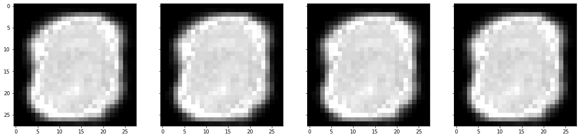
(a)

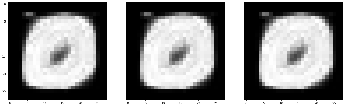
(b)

Figure 2: The sample fixed points of an autoencoder with hyperbolic tangent activation functions and nonnegative weights and biases on (a) the full MNIST dataset and (b) the ZERO dataset.

6.3 Tanh PN

In this setup, we modified slightly the autoencoder $T$ in Section 6.2 by clipping the negative coefficients of the weights in the training to 0.001 instead of 0. The resulting autoencoder $T$ has a primitive Jacobian matrix evaluated at a fixed point of $T$, hence, by Lemma 26 and Remark 23, such an autoencoder is both lower- and upper-primitive on the whole $\operatorname{Fix}({T}).$ Thus, from Proposition 22, we obtain that $\operatorname{Fix}({T})$ is an interval and that the fixed point iteration of $T$ converges to $u\in\operatorname{Fix}({T})$ for any positive starting point $x_{1}\gg 0.$ Figure 3 depicts fixed points of $T$ obtained for various positive starting points of the fixed point iteration. We note that the fixed points are very similar to the fixed points obtained for the autoencoder in Section 6.2.

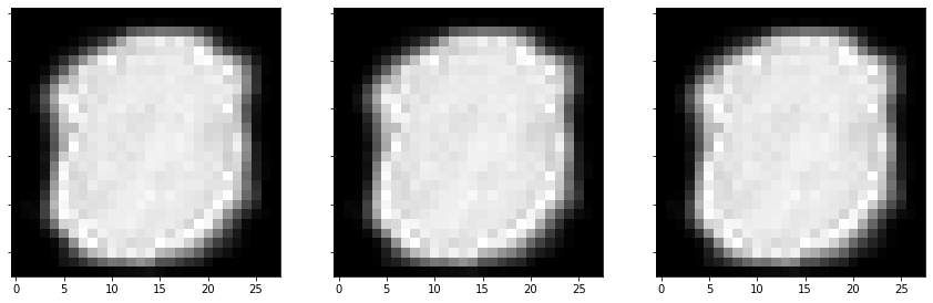
(a)

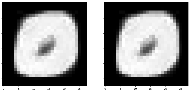
(b)

Figure 3: The sample fixed points of an autoencoder with a primitive Jacobian, positive weights, nonnegative biases, and hyperbolic tangent activation functions on (a) the full MNIST dataset and (b) the ZERO dataset.

6.4 ReLU spectral NN

In this setup, the autoencoder $T$ used the ReLU activation function in both layers. Thus, according to Corollary 9, $T$ is an $(A_{0,1,2})$-neural network. The ReLU activation function is in list (L2) in Remark 6, hence, from Proposition 11, point 2, and Corollary 13, the spectral radius of $T$ is $\rho(T_{\infty})=\max\{\lambda\in\mathbb{R}_{+}:\ \prod_{i=n}^{1}W_{i}x=\lambda x\}.$ After training, we obtained a neural network $T$ with $\rho(T_{\infty})=1.01>1$ for both the MNIST and ZERO datasets. In such a case, according to (Cavalcante and Stańczak, 2019, Proposition 2), the fixed-point of $T$ may only exist on the boundary of the cone. Indeed, we have numerical evidence that, in this case, the only fixed point of $T$ is the zero vector. Moreover, the obtained autoencoder had a high test loss compared to other setups. Therefore, to obtain a nondegenerate fixed point set of $T$, we enforced the spectral radius of the autoencoder to be less than 1 using spectral normalization Miyato et al. (2018), which normalizes all weight values by the largest singular value of the weight matrix. Indeed, the spectral radius obtained by the autoencoder $T$ trained with spectral normalization on the MNIST dataset is $\rho(T_{\infty})=0.93$ and on the ZERO dataset is $\rho(T_{\infty})=0.91$. Thus, from Corollary 14, $T$ has at least one fixed point. Moreover, it follows from Fact 31 that the least fixed point of $T$ can be computed with the fixed point iteration of $T$ starting at $x_{1}=0.$ We have also checked that the other fixed points of $T$ can be obtained for different positive starting points of the fixed point iteration of $T.$ However, similarly to the Tanh NN autoencoder in Section 6.2 above, the sufficient condition of lower- and upper-primitivity of $T$ at its fixed point given in Lemma 26 was not satisfied by $T$, thus the shape of the fixed point set of $T$ could not be determined. Numerically, the fixed points obtained in the MNIST and ZERO datasets are shown in Figure 4. For this case under consideration, the shape of the fixed point set is probably an interval, but, as already mentioned, at this moment there is no theory to prove formally this claim.

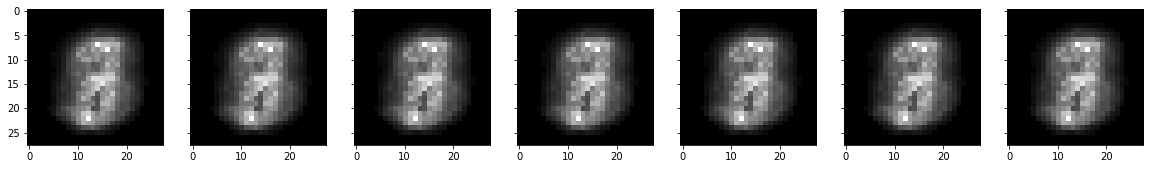
(a)

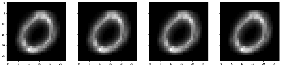
(b)

Figure 4: The sample fixed points of an autoencoder with nonnegative weights and biases, and ReLU activation functions using spectral normalization on (a) the MNIST dataset and (b) the ZERO dataset.

6.5 ReLU spectral PN

In this setup, we modified slightly the autoencoder $T$ in Section 6.4 by clipping the negative coefficients of the weights during training to 0.001 instead of 0. The resulting autoencoder $T$ has a primitive Jacobian matrix evaluated at a fixed point of $T$, hence, by Lemma 26 and Remark 23, such an autoencoder is both lower- and upper-primitive on the whole $\operatorname{Fix}({T}).$ Thus, from Proposition 22, we conclude that $\operatorname{Fix}({T})$ is an interval and that the fixed point iteration of $T$ converges to some $u\in\operatorname{Fix}({T})$ for any positive starting point $x_{1}\gg 0.$ Figure 5 presents sample fixed points of $T$ obtained for various positive starting points of the fixed point iteration.

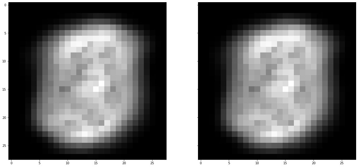
(a)

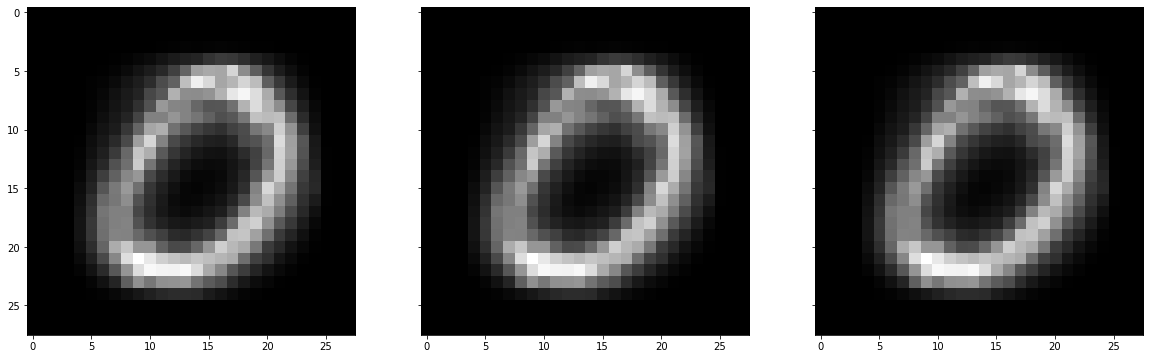
(b)

Figure 5: The sample fixed points of an autoencoder with primitive Jacobian, positive weights, nonnegative biases, and ReLU activation functions on (a) the MNIST dataset and (b) the ZERO dataset.

6.6 Tanh + Swish NN

In this setup, the autoencoder $T_{2}$ used the hyperbolic tangent activation functions in the first layer and the Swish activation functions in the second layer. Such an autoencoder satisfies Assumption 29 for $S=\emptyset$ and $P=\{1,2\}$, and thus it is an $(A_{0,1})$-neural network by Corollary 30. Then, following Example 4, this autoencoder is pointwise upper-bounded by an autoencoder $L$ constructed by replacing the Swish activation functions with the ReLU activation functions in the second layer, and we verify that $L$ is an $(A_{0,1,2})$-neural network. Therefore, using Proposition 11 and Corollary 13, we obtain that $\rho(L_{\infty})=0$, and, consequently, from Corollary 14 we know that $\operatorname{Fix}({L})\neq\emptyset.$ Hence, from Fact 34, we conclude that the autoencoder $T_{2}$ has at least one fixed point, and, from Fact 31, we obtain that the least fixed point of $T_{2}$ is the limit of the sequence constructed via the fixed point iteration of $T_{2}$ starting at $x_{1}=0.$ We have also checked that the other fixed points of $T_{2}$ can be obtained for different positive starting points of the fixed point iteration of $T_{2}.$ The sample fixed points obtained for $T_{2}$ are depicted in Figure 6.

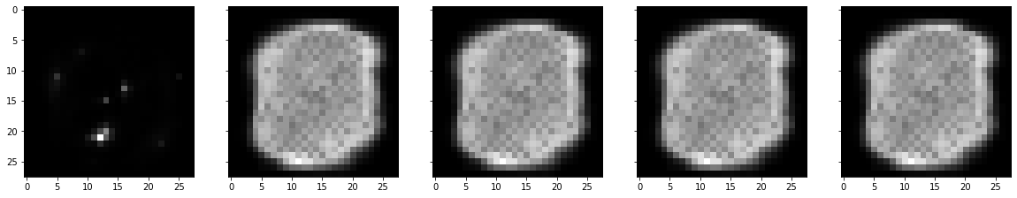
(a)

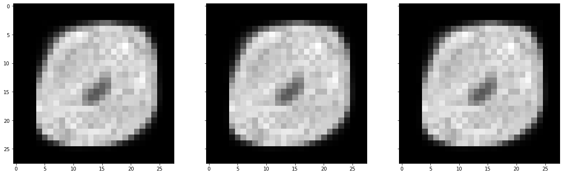
(b)

Figure 6: The sample fixed points of an autoencoder with nonnegative weights and biases, and with hyperbolic tangent and Swish activation functions on (a) the MNIST dataset and (b) the ZERO dataset.

6.7 ReLU + Sigmoid NR

In this setup, the autoencoder $T_{2}$ had nonnegative weights and real-valued biases, and it used ReLU activation functions in the first layer and sigmoid activation functions in the second layer. Such an autoencoder satisfies Assumption 29 for $S=\{1,2\}$ and $P=\emptyset$, and thus it is an $(A_{0,1})$-neural network by Corollary 30. Then, following Example 3, such an autoencoder is pointwise upper-bounded by the autoencoder $L$ with the same structure but with negative biases replaced with zeros. By doing so, $L$ is an $(A_{0,1,2})$-neural network. Therefore, using Proposition 11 and Corollary 13, we verify that $\rho(L_{\infty})=0$. Consequently, from Corollary 14 we deduce that $\operatorname{Fix}({L})\neq\emptyset.$ Hence, from Fact 34 we conclude that the autoencoder $T_{2}$ has at least one fixed point, and, from Fact 31, we know that the least fixed point of $T_{2}$ can be computed using the fixed point iteration of $T_{2}$ starting at $x_{1}=0.$ We have also checked that the other fixed points of $T_{2}$ can be computed for different positive starting points of the fixed point iteration of $T_{2}.$ The sample fixed points obtained for $T_{2}$ are depicted in Figure 7.

(a)

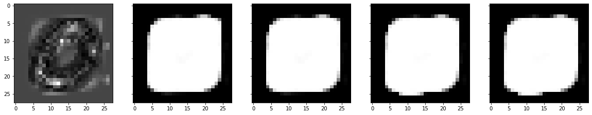
(b)

Figure 7: The sample fixed points of an autoencoder with only nonnegative weights, and with ReLU and sigmoid activation functions on (a) the MNIST dataset and (b) the ZERO dataset.

6.8 ReLU + Sigmoid RR

In this setup, the autoencoder $T_{2}$ had real-valued weights and biases, and it used ReLU activation functions in the first layer and sigmoid activation functions in the second layer. Thus, the autoencoder satisfies Assumption 32, and, hence, by Corollary 33, $T_{2}$ is an $(A_{0})$-neural network. By replacing negative weights and biases with zeros, we obtain from Corollary 9 an $(A_{0,1,2,3})$-neural network $L$ that upper-bounds $T_{2}$. From Proposition 11 and Corollary 13, we have that $\rho(L_{\infty})=0$, and, from Corollary 15, we conclude that $L$ has a unique and positive fixed point. We note that $L$ is in particular an $(A_{0,1})$-neural network, which follows from the relations $(A_{0,1,2,3})\subset(A_{0,1,2})\subset(A_{0,1}).$ Therefore, using Fact 34 and Remark 35, we conclude that $\operatorname{Fix}({T_{2}})\neq\emptyset.$ However, as stated in Remark 36, the fixed point iteration of $T_{2}$ does not necessarily converge to its fixed point. Indeed, using the fixed point iteration of $T_{2}$ for various starting points, we obtained fixed points for the MNIST dataset, but not for the ZERO dataset. The sample fixed points obtained on the MNIST dataset are depicted in Figure 8.

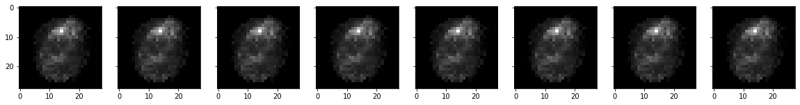
Figure 8: The sample fixed points of an autoencoder with real-valued weights and biases on the MNIST dataset.

Table 1: Spectral radii, products of weight matrices spectral norms, spectral norms of products of weight matrices, and test loss on the MNIST dataset for different configurations of autoencoders.

Configuration	Test loss	$\rho(T_{\infty})$	$\|W_{1}\|\cdot\|W_{2}\|$	$\|W_{2}\cdot W_{1}\|$
Sigmoid NN 6.1	0.2308	0.00	7.271	6.052
Tanh NN 6.2	0.0065	0.00	463.9	187.3
Tanh PN 6.3	0.0255	0.00	40.63	35.85
ReLU spectral NN 6.4	0.0063	0.98	1.072	0.999
ReLU spectral PN 6.5	0.0059	0.99	1.0006	1.0001
Tanh + Swish NN 6.6	0.0041	—	15.221	8.8120
ReLU + Sigmoid NR 6.7	0.0025	—	2845.3	215.13
ReLU + Sigmoid RR 6.8	0.0052	—	3196.9	332.97

Below, we discuss possible future research directions, based on analytic and simulation results of previous sections.

7 Research directions

Current studies indicate that obtaining simple and general results about the shape of the fixed point set of generic $(A_{0,1})$-neural networks might be a difficult task. As an example, a very recent result Reich and Zaslavski (2023) shows that, even for the simple case of $(A_{1})$ (continuous and monotonic) self-mappings defined on an interval $[a,b]$, i.e., nondecreasing functions $f\colon[a,b]\to[a,b]$, the problem of determining explicitly $\operatorname{Fix}({f})$ is a highly non-trivial task. In particular, (Reich and Zaslavski, 2023, Theorem 2.2) asserts that, for any integer $n\geq 2$, there exists an open and everywhere dense set of such functions for which the cardinality of $\operatorname{Fix}({f})$ is lower bounded by $n$. Furthermore, any uniqueness conditions on fixed points of $(A_{0,1,2})$-mappings, beyond those presented in this paper, must clearly preclude simple cases such as the identity mapping $Id\colon\mathbb{R}^{k}_{+}\to\mathbb{R}^{k}_{+}$, which is the simplest example of an $(A_{0,1,2})$-mapping with an uncountable number of fixed points ($\operatorname{Fix}({Id})=\mathbb{R}^{k}_{+}$).

Two additional important questions, especially from an application perspective, are the following:

1. determine the sets of approximate fixed points, that is, find $x\in\mathbb{R}^{k}_{+}$ such that $T(x)\approx x$ (in some sense), where $T$ is the nonnegative neural network under consideration; and

2. lift the restriction of nonnegative inputs and outputs.

Below we discuss potential research directions toward these goals.

7.1 Approximate fixed points

In the previous sections, we have established the simplicity of fixed points sets of $(A_{0,1,2})$- and $(A_{0,1,2,3})$-neural networks, and we have also obtained reasonably good performance of nonnegative autoencoders with different architectures in simulations. A promising research direction is to address two hypotheses discussed in the Introduction (Section 1); namely, that only “sufficiently good” performance is all we should expect from a nonnegative self-mapping neural network, and that perfection is in practice neither desirable nor achievable. The approaches described in the next two subsections may serve as starting points.

7.1.1 Slow convergence to fixed points

The fixed points obtained in the simulations in Section 6 on the MNIST dataset frequently resemble a noisy average of input classes. We may also consider the input-output relation $x\mapsto T(x)$ of a nonnegative autoencoder $T$ as the first iteration of the fixed point algorithm $x_{n+1}\stackrel{{\scriptstyle\mathclap{\tiny\mbox{df.}}}}{{=}}T^{n}(x)$ for $n\in\mathbb{N}.$ As a result, an autoencoder $T$ is expected to provide good reconstruction performance ($x\approx T(x)$) if the fixed point algorithm $x_{n+1}=T^{n}(x)$ is slow. Based on this viewpoint of fixed point theory, a natural strategy for improving the performance of autoencoders is to design them in a way that guarantees slow convergence of their fixed point iterations. We now show that the theory described in the study gives rise to simple heuristics with some analytical justification to achieve this goal.

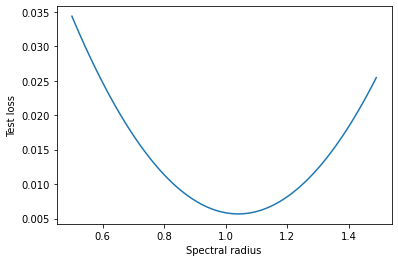
Figure 9: Dependence of the test loss on the spectral radius of the ReLU spectral PN autoencoder described in Section 6.5.

For the special case of a positive concave autoencoder $T$, which belongs to the subclass of $(A_{0,1,2,3})$-autoencoders, the result in (Piotrowski and Cavalcante, 2022, Remark 8) shows the explicit factor $c\in[0,1)$ of geometric convergence of the fixed point iteration of $T$ to its unique fixed point. The closer $c$ is to one, the slower the convergence speed of the fixed point algorithm is expected to be, and, hence, the better reconstruction performance we may expect from the autoencoder. In particular, the contraction $c$ is lower bounded by the spectral radius $\rho(T_{\infty})$ (Piotrowski and Cavalcante, 2022, Proposition 4). Furthermore, if $\rho(T_{\infty})>0$, it follows from (12) that we can modify the autoencoder $T$ to have its spectral radius to an arbitrary nonnegative value $u$ by simply scaling the weights of the first layer by $u/\rho(T_{\infty})$. In Figure 9, we extrapolated heuristically this procedure to the $(A_{0,1,2})$-ReLU spectral PN autoencoder considered in Section 6.5, and we verify that the test loss indeed achieves its minimum value if the spectral radius is close to one. More precisely, if $1-\epsilon<c<1$ for some sufficiently small $\epsilon>0$, we may expect slowly converging fixed point iterations. On the other hand, if $1\leq c<1+\epsilon$, Figure 9 suggests that autoencoders with possibly slowly diverging fixed point iterations are also able to produce good approximate fixed points.

7.1.2 Lipschitz continuity

Continuing our quest for good reconstruction performance (informally defined as $T(x)\approx x$) of nonnegative autoencoders, we may aim at exploiting continuity of the neural networks. Unfortunately, simple properties such as Lipschitz continuity are not likely to succeed because the best Lipschitz constant can be prohibitively large. More precisely, the result in (Combettes and Pesquet, 2020a, Section 2) shows that all activation functions from lists (L1)-(L2) in Remark 6 are nonexpansive in a Hilbert space. Thus, from (Combettes and Pesquet, 2020b, Proposition 4.3), we deduce that neural networks satisfying the conditions in Definitions 3-4, and, in particular, those considered in Sections 3-5, are Lipschitz-continuous, and the corresponding Lipschitz constant $\theta$ can be bounded by

$$\|\prod_{i=n}^{1}W_{i}\|\leq\theta\leq\prod_{i=1}^{n}\|W_{i}\|.$$ (18)

As Table 1 at the end of Section 6 shows, for $n=2$ the lower bound $\|\prod_{i=n}^{1}W_{i}\|$ (achievable by neural networks with nonnegative weights, see (Combettes and Pesquet, 2020b, Section 5.3)) is too large to obtain meaningful bounds for $\|T(x)-x\|$ around its fixed point(s) $x^{\star}\in\operatorname{Fix}({T})$. Therefore, a more subtle argument, perhaps based on local Lipschitz continuity at input classes, should be considered for exploiting the continuity of $T$ with the aim of finding $x$ such that $T(x)\approx x.$

7.2 Extending current results beyond nonnegativity

This study mostly focuses on monotonic neural networks with nonnegative inputs and outputs, but a well-known pre- and post-processing step enables us to extend the above results to a particular class of monotonic neural networks with inputs and outputs possibly taking values in the whole real line. More precisely, let $T:\operatorname{int}(\mathbb{R}^{k}_{+})\to\operatorname{int}(\mathbb{R}^{k}_{+})$ be a neural network with a structure that can be analyzed with the theory in this study. To train and operate a neural network of this type with inputs and outputs taking values in $\mathbb{R}^{k}$, we can proceed as follows. Let $L:\operatorname{int}(\mathbb{R}^{k}_{+})\to\mathbb{R}^{k}:x\mapsto[\log(x_{1}),\ldots,\log(x_{k})]$ and $E:\mathbb{R}^{k}\to\operatorname{int}(\mathbb{R}^{k}_{+}):x\mapsto[\exp(x_{1}),\ldots,\exp(x_{k})]$ denote, respectively, the coordinate-wise log and exponential mappings. Now, consider the neural network defined by $N:\mathbb{R}^{k}\to\mathbb{R}^{k}:x\mapsto L(T(E(x)))$; i.e., we first map an input in $\mathbb{R}^{k}$ to $\operatorname{int}(\mathbb{R}^{k}_{+})$ with the exponential mapping, process the mapped input with the original positive neural network $T$, and then map the output of $T$ back to $\mathbb{R}^{k}$ with the log mapping. Some properties of $N$ can be directly deduced from $T$. For example, we verify that $N$ has a fixed point if and only if $T$ also has a fixed point. Furthermore, the uniqueness of the fixed point of $T$ implies the uniqueness of the fixed point of $N$. These are all properties that can be verified with the theory described in the previous sections. From a mathematical perspective, the mapping $L$ is the known isometry between Thompson’s metric space $(\operatorname{int}({\mathbb{R}^{k}_{+}}),d_{T})$ (see Definition 37) and the normed vector space $(\mathbb{R}^{k},~{}\|\cdot\|_{\infty})$, and further properties of the neural network $N$ are strongly connected to the theory of topical mappings (Lemmens and Nussbaum, 2012, Sect. 1.5).

8 Conclusion

We have shown that the behavior of many neural networks that can be seen as self-mappings with nonnegative weights (as often proposed in the literature) can be rigorously analyzed with the framework of nonlinear Perron-Frobenius theory. We also demonstrated that the concept of the spectral radius of asymptotic mappings is useful for determining whether a neural network has an empty or nonempty fixed point set, and, for an autoencoder, we recall that its fixed point set corresponds to the inputs that can be perfectly reconstructed at the output. Our conditions for the existence of fixed points of nonnegative neural networks are weaker than those previously considered in the literature, which are often based on arguments in convex analysis in Hilbert spaces. Our theoretical results also open new and possibly interesting research questions, such as the existence of “approximate” fixed points, which may be extremely useful in practical applications of nonnegative neural networks such as nonnegative autoencoders.

Appendix A Known results

Definition 37

We define Thompson’s metric by

$$\begin{array}[]{rl}d_{T}:\operatorname{int}({\mathbb{R}^{k}_{+}})\times\operatorname{int}({\mathbb{R}^{k}_{+}})&\to[0,\infty)\\ (x,y)&\mapsto\ln(\max\{M(x,y),M(y,x)\}),\end{array}$$ (19)

where

$$\begin{array}[]{rl}M:\operatorname{int}({\mathbb{R}^{k}_{+}})\times\operatorname{int}({\mathbb{R}^{k}_{+}})&\to[0,\infty)\\ (x,y)&\mapsto\inf\{\beta>0~{}|~{}x\leq\beta y\}.\end{array}$$

We call the metric space $(\operatorname{int}({\mathbb{R}^{k}_{+}}),d_{T})$ the Thompson metric space.

Proposition 38 ((Cavalcante and Stańczak, 2019, Proposition 1))

Let $T\colon\mathbb{R}^{k}_{+}\to\mathbb{R}^{k}_{+}$ be an $(A_{0,1,2})$-mapping. If $\rho(T_{\infty})<1$, then $\operatorname{Fix}({T})\neq\emptyset.$

Proposition 39 ((Cavalcante et al., 2019, Proposition 4))

Let $T\colon\mathbb{R}^{k}_{+}\to\operatorname{int}(\mathbb{R}^{k}_{+})$ be an $(A_{0,1,2,3})$-mapping. Then $\operatorname{Fix}({T})\neq\emptyset$ if and only if $\rho(T_{\infty})<1.$

Proposition 40 ((Cavalcante et al., 2019, Fact 1(ii)))

Let $T\colon\mathbb{R}^{k}_{+}\to\mathbb{R}^{k}_{+}$ be an $(A_{0,1,2,3})$-mapping. Then $\operatorname{Fix}({T})\neq\emptyset$ is either a singleton or the empty set.

Appendix B Construction of monotonic and weakly scalable functions

The following general lemma introduces building blocks to construct $(A_{0,1,2})$-mappings, or even $(A_{0,1,2,3})$-mappings. It extends (Oshime, 1992, Proposition 2.3) to functions that are not necessarily self-mappings.

Lemma 41

  

1. Let $f_{1}\colon\mathbb{R}^{s}_{+}\to\mathbb{R}^{p}_{+}$ and $f_{2}\colon\mathbb{R}^{s}_{+}\to\mathbb{R}^{p}_{+}$ be $(A_{0})$-mappings and let $\alpha,\beta\geq 0.$ Consider the following mappings:

   $$x\mapsto(\alpha f_{1}+\beta f_{2})(x),$$ (20)

   $$x\mapsto\max\{f_{1},f_{2}\}(x),$$ (21)

   $$x\mapsto\min\{f_{1},f_{2}\}(x).$$ (22)

   Then we have:

   1. If $f_{1},f_{2}$ are $(A_{0,1})$-mappings, then so are the mappings in (20)-(22).

   2. If $f_{1},f_{2}$ are $(A_{0,1,2})$-mappings, then so are the mappings in (20)-(22).

   3. If $f_{1}$ in as $(A_{0,1,2})$-mapping and $f_{2}$ is an $(A_{0,1,2,3})$-mapping, $\alpha\geq 0$ and $\beta>0$, then the function in (20) is an $(A_{0,1,2,3})$-mapping.

   4. if $f_{1},f_{2}$ are $(A_{0,1,2,3})$-mappings, then so are the mappings in (21)-(22).

2. Let $g\colon\mathbb{R}^{p}_{+}\to\mathbb{R}^{r}_{+}$ be an $(A_{0})$-mapping and consider the following mapping:

   $$x\mapsto(g\circ f_{1})(x).$$ (23)

   1. If $f_{1},g$ are $(A_{0,1})$-mappings, then so is the function in (23).

   2. If $f_{1},g$ are strictly monotonic, then so is the function in (23).

   3. If $f_{1},g$ are strongly monotonic, then so is the function in (23).

   4. If $f_{1}$ is an $(A_{0,2})$-mapping and $g$ is an $(A_{0,1,2})$-mapping, then the mapping in (23) is an $(A_{0,2})$-mapping.

   5. If $f_{1}$ is an $(A_{0,2})$-mapping and $g$ is an $(A_{0,1,2,3})$-mapping, then the mapping in (23) is an $(A_{0,2,3})$-mapping.

   6. If $f_{1}$ is an $(A_{0,2,3})$-mapping, and $g$ is a strictly monotonic $(A_{0,2})$-mapping, then the mapping in (23) is an $(A_{0,2,3})$-mapping.

Proof

Part 1: Properties of mappings in (20)-(22)

1.(a)

Let $x,\tilde{x}\in\mathbb{R}^{s}_{+}$ be such that $x\leq\tilde{x}$, let $\alpha,\beta\geq 0$, and let $f_{1},f_{2}$ be $(A_{0,1})$-mappings. Then $\alpha f_{1}(x)\leq\alpha f_{1}(\tilde{x})$ and $\beta f_{2}(x)\leq\beta f_{2}(\tilde{x}).$ By adding these two inequalities we obtain monotonicity of $x\mapsto(\alpha f_{1}+\beta f_{2})(x).$ Furthermore, we also have $\max\{f_{1},f_{2}\}(x)\leq\max\{f_{1},f_{2}\}(\tilde{x})$ and $\min\{f_{1},f_{2}\}(x)\leq\min\{f_{1},f_{2}\}(\tilde{x}).$

1.(b)

Let $x\in\mathbb{R}^{s}_{+}$, let $\alpha,\beta\geq 0$, and let $f_{1},f_{2}$ be $(A_{0,1,2})$-mappings. Fix $\rho\geq 1.$ Then $\alpha f_{1}(\rho x)\leq\alpha\rho f_{1}(x)$ and $\beta f_{2}(\rho x)\leq\beta\rho f_{2}(x).$ By adding these two inequalities we obtain weak scalability of $x\mapsto(\alpha f_{1}+\beta f_{2})(x).$ Furthermore, we have $\max\{f_{1},f_{2}\}(\rho x)\leq\max\{\rho f_{1},\rho f_{2}\}(x)=\rho\max\{f_{1},f_{2}\}(x)$, with the same arguments for weak scalability of $\min\{f_{1},f_{2}\}(\rho x).$

1.(c)

Let $f_{1}$ be an $(A_{0,1,2})$-mapping and $f_{2}$ be an $(A_{0,1,2,3})$-mapping, with $\alpha\geq 0$ and $\beta>0$, and let $\rho>1.$ Then $\alpha f_{1}(\rho x)\leq\alpha\rho f_{1}(x)$ and $\beta f_{2}(\rho x)\ll\beta\rho f_{2}(x).$ By adding these two inequalities we obtain scalability of $x\mapsto(\alpha f_{1}+\beta f_{2})(x).$

1.(d)

We have $\max\{f_{1},f_{2}\}(\rho x)\ll\max\{\rho f_{1},\rho f_{2}\}(x)=\rho\max\{f_{1},f_{2}\}(x)$, with the same arguments for scalability of $\min\{f_{1},f_{2}\}(\rho x).$

Part 2: Properties of mapping in (23)

2.(a)

Let $x,\tilde{x}\in\mathbb{R}^{s}_{+}$ be such that $x\leq\tilde{x}$ and let $f_{1},g$ be $(A_{0,1})$-mappings. Then $f_{1}(x)\leq f_{1}(\tilde{x})$, and, hence, $g(f_{1}(x))\leq g(f_{1}(\tilde{x})).$

2.(b) and 2.(c)

As above.

2.(d)

Let $x\in\mathbb{R}^{s}_{+}$, and let $f_{1}$ be an $(A_{0,2})$-mapping and $g$ be an $(A_{0,1,2})$-mapping. Fix $\rho\geq 1.$ From weak scalability of $f_{1}$, we have $f_{1}(\rho x)\leq\rho f_{1}(x)$, and, from monotonicity of $g$, we deduce $g(f_{1}(\rho x))\leq g(\rho f_{1}(x)).$ Weak scalability of $g$ yields $g(\rho f_{1}(x))\leq\rho g(f_{1}(x)).$

2.(e)

Let $x\in\mathbb{R}^{s}_{+}$, and let $f_{1}$ be an $(A_{0,2})$-mapping and $g$ be an $(A_{0,1,2,3})$-mapping. Fix $\rho>1.$ As above, we have $g(f_{1}(\rho x))\leq g(\rho f_{1}(x)).$ Then, from scalability of $g$, it follows that $g(\rho f_{1}(x))\ll\rho g(f_{1}(x)).$

2.(f)

Let $x\in\mathbb{R}^{s}_{+}$, and let $f_{1}$ be an $(A_{0,2,3})$-mapping, and $g$ be a strictly monotonic $(A_{0,2})$-mapping. Fix $\rho>1.$ By our assumptions, we have $f_{1}(\rho x)\ll\rho f_{1}(x)$, and, from strict monotonicity of $g$, we have $g(f_{1}(\rho x))\ll g(\rho f_{1}(x)).$ Weak scalability of $g$ implies $g(\rho f_{1}(x))\leq\rho g(f_{1}(x))$, and the proof is completed. $\blacksquare$

Appendix C Proof of Lemma 8

Proof We use the results of Lemma 41 to prove points 1)-7) as follows:

1) Put $f_{1}(x)=Wx$ and $g(x)=x+b$, and note that $f_{1}$ is an $(A_{0,1,2})$-mapping if $W$ is nonnegative, whereas $g$ is a strictly monotonic $(A_{0,2})$-mapping for $b\geq 0.$ Then, from 2(a) in Lemma 41, the affine function $y_{i}=W_{i}x_{i-1}+b_{i}$ is monotonic, and from 2(d) in Lemma 41, it is also weakly scalable.

2) From point 1) we have that $y_{i}=W_{i}x_{i-1}+b_{i}$ is an $(A_{0,1,2})$-mapping. To prove scalability, we note that, if $b\gg 0$, then $g(x)=x+b$ is a strictly monotonic $(A_{0,2,3})$-mapping. The desired assertion now follows from 2(e) in Lemma 41.

3) Monotonicity of $T_{i}$ follows from 2(a) in Lemma 41 and its weak scalability from 2(d) in Lemma 41.

4) Monotonicity of $T_{i}$ follows from point 3) above. Scalability of $T_{i}$ follows from 2(e) in Lemma 41.

5) Monotonicity of $T_{i}$ follows from point 3) above. Scalability of $T_{i}$ follows from 2(f) in Lemma 41.

6) Monotonicity and weak scalability of $T$ follows from, respectively, an application of 2(a) and 2(d) in Lemma 41 to consecutive layers of $T.$

7) Monotonicity of $T$ follows from point 6) above. To prove scalability, verify from 2(e) in Lemma 41 that a subnetwork of $T$ composed of the first $i_{0}$ layers of $T$ is scalable. Scalability of $T$ now follows from an application of 2(f) in Lemma 41 to consecutive layers of $T$, starting with the $i_{0}+1$-st layer. $\blacksquare$

References

- Adler and Öktem (2017) J. Adler and O. Öktem. Solving ill-posed inverse problems using iterative deep neural networks. Inverse Problems, 33(12):124007, 2017.
- Ali and Yangyu (2017) Afan Ali and Fan Yangyu. Automatic modulation classification using deep learning based on sparse autoencoders with nonnegativity constraints. IEEE Signal Processing Letters, 24(11):1626–1630, 2017.
- Arbib and Bonaiuto (2016) M. A. Arbib and J. J. Bonaiuto. From Neuron to Cognition via Computational Neuroscience. MIT Press, 2016.
- Ayinde and Zurada (2018) Babajide O Ayinde and Jacek M Zurada. Deep learning of constrained autoencoders for enhanced understanding of data. IEEE Transactions on Neural Networks and Learning Systems, 29(9):3969–3979, 2018.
- Benning and Burger (2018) M. Benning and M. Burger. Modern regularization methods for inverse problems. Acta Numerica, 27:1–111, May 2018.
- Boche and Schubert (2008) Holger Boche and Martin Schubert. Concave and convex interference functions—general characterizations and applications. IEEE Transactions on Signal Processing, 56(10):4951–4965, 2008.
- Boyd and Vandenberghe (2006) S. Boyd and L. Vandenberghe. Convex Optimization. Cambridge Univ. Press, Cambridge, U.K., 2006.
- Burbanks et al. (2003) A. D. Burbanks, R. D. Nussbaum, and C. T. Sparrow. Extensions of order-preserving maps on a cone. Proc. Royal Society of Edinburgh Sect.A, 133(1):35–59, 2003.
- Cavalcante and Stańczak (2019) R. L. G. Cavalcante and S. Stańczak. Weakly standard interference mappings: Existence of fixed points and applications to power control in wireless networks. In ICASSP 2019 - 2019 IEEE International Conference on Acoustics, Speech and Signal Processing (ICASSP), pages 4824–4828, 2019.
- Cavalcante et al. (2014) R. L. G. Cavalcante, S. Stańczak, M. Schubert, A. Eisenbläter, and U. Türke. Toward energy-efficient 5G wireless communication technologies. IEEE Signal Processing Mag., 31(6):24–34, Nov. 2014.
- Cavalcante et al. (2017) R. L. .G. Cavalcante, M. Kasparick, and S. Stańczak. Max-min utility optimization in load coupled interference networks. IEEE Trans. Wireless Commun., 16(2):705–716, Feb. 2017.
- Cavalcante et al. (2019) R. L. G. Cavalcante, Q. Liao, and S. Stańczak. Connections between spectral properties of asymptotic mappings and solutions to wireless network problems. IEEE Transactions on Signal Processing, 67(10):2747–2760, 2019.
- Cavalcante et al. (2016) Renato L. G. Cavalcante, Yuxiang Shen, and Sławomir Stańczak. Elementary properties of positive concave mappings with applications to network planning and optimization. IEEE Transactions on Signal Processing, 64(7):1774–1783, 2016.
- Chen et al. (2019) Y. Chen, Y. Shi, and B. Zhang. Optimal control via neural networks: a convex approach. In The International Conference on Learning Representations (ICLR), 2019.
- Chorowski and Zurada (2015) Jan Chorowski and Jacek M Zurada. Learning understandable neural networks with nonnegative weight constraints. IEEE Transactions on Neural Networks and Learning Systems, 26(1):62–69, 2015.
- Combettes and Pesquet (2020a) P. L. Combettes and J.-C. Pesquet. Deep neural network structures solving variational inequalities. Set-Valued and Variational Analysis, 28:491–518, September 2020a.
- Combettes and Pesquet (2020b) P. L. Combettes and J.-C. Pesquet. Lipschitz certificates for layered network structures driven by averaged activation operators. SIAM Journal on Mathematics of Data Science, 2(2):529–557, June 2020b.
- Doya et al. (2007) K. Doya, S. Ishii, A. Pouget, and R. P. N. Rao, editors. Bayesian Brain: Probabilistic Approaches to Neural Coding. MIT Press, 2007.
- Goodfellow et al. (2016) I. Goodfellow, Y. Bengio, and A. Courville. Deep Learning. The MIT Press, Cambridge, Massachusetts, 2016.
- Hosseini-Asl et al. (2015) Ehsan Hosseini-Asl, Jacek M Zurada, and Olfa Nasraoui. Deep learning of part-based representation of data using sparse autoencoders with nonnegativity constraints. IEEE Transactions on Neural Networks and Learning Systems, 27(12):2486–2498, 2015.
- Johnson and Bru (1990) Charles R. Johnson and Rafael Bru. The spectral radius of a product of nonnegative matrices. Linear Algebra and its Applications, 141:227–240, 1990.
- Kendall et al. (2020) Jack Kendall, Ross Pantone, Kalpana Manickavasagam, Yoshua Bengio, and Benjamin Scellier. Training end-to-end analog neural networks with equilibrium propagation. 2020. arXiv:2006.01981 [cs.NE].
- Krause (2015) Ulrich Krause. Positive dynamical systems in discrete time: theory, models, and applications, volume 62. Walter de Gruyter GmbH & Co KG, 2015.
- LeCun et al. (2015) Y. A. LeCun, Y. Bengio, and G. Hinton. Deep learning. Nature, 521:436–444, 2015.
- Lee and Seung (1999) D. D. Lee and H. S. Seung. Learning the parts of objects by nonnegative matrix factorization. Nature, 401(6755):788–791, 1999.
- Lemme et al. (2012) Andre Lemme, René Felix Reinhart, and Jochen Jakob Steil. Online learning and generalization of parts-based image representations by non-negative sparse autoencoders. Neural Networks, 33:194–203, 2012.