Influence of Roughening Transition on Magnetic Ordering

Abstract

In the literature of magnetic phase transitions, in addition to a critical point, existence of another special point has been discussed. This is related to the broadening of interface between two different ordering phases and is referred to as the point of roughening transition. While there exists good understanding on equilibrium properties associated with this transition, influence of this on nonequilibrium dynamics has not been investigated. In this paper we present comprehensive results, from Monte Carlo simulations, on coarsening dynamics in a system, over a wide range of temperature, in space dimension $d=3$, for which there exists roughening transition at a nonzero temperature. State-of-the-art analysis of the simulation data, on structure, growth and aging, shows that the onset of unexpected glass-like slow dynamics in this system, that has received much attention in recent times, for quenches to zero temperature, actually occurs at this transition point. This demonstrates an important structure-dynamics connection in phase-ordering dynamics. We compare the key results with those from $d=2$, for which there exists no non-zero roughening transition temperature. Absence of the above mentioned anomalous features in the latter dimension places our conjecture on the role of roughening transition on a firmer footing.

I Introduction

Over past several decades there has been significant interest spirin1 ; spirin2 ; oliveira ; kondrat ; arenzon ; olejarz1 ; olejarz2 ; olejarz3 ; corberi ; blanchard ; blanchard2 ; amar ; shore ; cueille ; das1 ; das2 ; das3 ; denholm ; godriche ; mullick ; yu ; cugliandolo ; liu ; ohta ; yeung2 in the understanding of ordering dynamics following quenches of paramagnetic configurations to the ferromagnetic region by crossing the critical temperature mfisher1 $T_{c}$. In recent times glass-like dynamics in a popular ordering system, despite the absence of in-built frustration, following quenches to the final temperature $T_{f}=0$, drew attention olejarz1 ; olejarz2 ; olejarz3 ; blanchard ; blanchard2 ; shore ; cueille ; das1 ; das2 ; das3 . This slow dynamics perhaps is due to non-conventional structure formation. The observation is striking and it is unknown whether such unexpected behavior corberi ; das1 ; das2 ; das3 is specific to $T_{f}=0$. It is possible that the origin is at the roughening transition beijern , that occurs at a much higher temperature $T_{R}$ $(<T_{c})$, given that below $T_{R}$ interfaces are sharp. Knowledge of this is crucial not only in the understanding of this intriguing fact but also in establishing structure-dynamics coupling in the general context of growth phenomena. Interestingly, the consequences of the presence or absence of rough interfaces, of importance in real systems, in such nonequilibrium phenomena has not been investigated, though the equilibrium aspects of roughening transition is reasonably well explored.

Some of the key aspects of ordering dynamics bray ; puri ; dfisher ; yeung1 ; henkel ; lorenz ; liu ; ohta ; das4 ; yeung2 ; huse ; das5 ; allen ; landau are: i) self-similarity and scaling property of structure, ii) growth of the latter, and iii) related aging. The structure is typically probed via the two-point equal time $(t)$ correlation function bray , which, for a spin system, reads $C(r,t)=\langle S_{i}(t)S_{j}(t)\rangle-\langle S_{i}(t)\rangle\langle S_{j}(t)\rangle$, $S_{i}$ and $S_{j}$ representing orientations of spins or atomic magnets at sites $i$ and $j$, located $r$ distance apart. It is also customary to study the Fourier transform of $C(r,t)$, the structure factor, $S(k,t)$, $k$ being the wave number bray . The latter has direct experimental relevance. These quantities obey certain scaling properties when the growth is self-similar. E.g., in simple situations, when structures are non-fractal, $C(r,t)$ satisfies bray $C(r,t)\equiv\tilde{C}(r/\ell)$, $\ell$ being the average domain size or characteristic length scale of the growing system at time $t$ and $\tilde{C}(x)$ a time-independent master function. In such a situation $\ell$ is expected bray to grow as $\sim t^{\alpha}$. A power-law behavior is expected for aging phenomena also. In the latter case the autocorrelation function puri ; dfisher , $C_{\textrm{ag}}(t,t_{w})=\langle S_{i}(t)S_{i}(t_{w})\rangle-\langle S_{i}(t)\rangle\langle S_{i}(t_{w})\rangle$, should scale as $\sim$ $(\ell/\ell_{w})^{-\lambda}$, in the asymptotic limit when $\ell>>\ell_{w}$. Here, $t_{w}$ $(\leq t)$ is the waiting time or age of the system and $\ell_{w}$ is the value of $\ell$ at $t=t_{w}$.

For uniaxial ferromagnets one expects bray ; allen $\alpha=1/2$. The structure in this case is supposed to be described by the Ohta-Jasnow-Kawasaki (OJK) function bray ; ohta : $C(r,t)=\frac{2}{\pi}\sin^{-1}[\exp(-r^{2}/Dt)]$, $D$ being a constant. Note that while the form of $C(r,t)$ and the value of growth exponent $\alpha$ are independent of space dimension $d$, aging exponent $\lambda$ changes with it. The values of $\lambda$ for this ordering, as obtained by Liu and Mazenko (LM) liu , are expected to be $\simeq 1.67=\lambda_{3}^{\rm{LM}}$ in $d=3$, whereas in $d=2$, it is $\lambda_{2}^{\rm{LM}}\simeq 1.29$. Unless otherwise mentioned, in the rest of the paper all our discussions are for $d=3$.

While these theoretical predictions were confirmed via the Monte Carlo landau simulations of the Ising model, for moderately high values of $T_{f}$, striking deviations were reported for $T_{f}=0$, in $d=3$. In the latter case, several works concluded that $\alpha=1/3$ or the growth is even slower. Most recently it was reported that the OJK function does not das3 describe the pattern at $T_{f}=0$. Furthermore, $\lambda$ was also estimated das3 to be much weaker than $\lambda_{3}^{\rm{LM}}$. Thorough investigations, we believe, are necessary, in order to arrive at a complete and correct picture. It needs to be understood if such anomalies bear any connection with any other special point. If such a special point turns out to be that of the roughening transition, important relation concerning structure and dynamics das6 can be established in the nonequilibrium context. Our study clearly suggests that the above mentioned anomalous features are not specific to $T_{f}=0$. The onset of the anomalies occurs at the roughening transition. The key results have been verified by sophisticated finite-size scaling analysis das4 ; mfisher2 ; das_pre_fss . We believe that these will inspire novel investigations, thereby explaining intriguing dynamical phenomena in the nonequilibrium domain.

II Model and Methods

We choose $J>0$ in the Ising Hamiltonian landau ; mfisher1 $H=-J\sum_{<ij>}S_{i}S_{j}$, where $S_{i}$ and $S_{j}$ can take values $+1$ and $-1$, corresponding to up and down orientations of the atomic magnets. We study this model on a simple cubic lattice, having $T_{c}\simeq 4.51J/k_{B}$ landau , where $k_{B}$ is the Boltzmann constant. For the limited set of results in $d=2$, we considered the square lattice. Note that in this case $T_{c}\simeq 2.27J/k_{B}$ landau . In $d=3$, the value of $T_{R}$ for this model is $\simeq 2.57J/k_{B}$ beijern , whereas a non-zero roughening transition temperature does not exist in $d=2$.

Moves in our MC simulations were tried by randomly choosing a spin and changing its sign landau ; glauber . These were accepted by following standard Metropolis criterion landau . Unit of time in our simulations is a MC step (MCS) that consists of $L^{d}$ trial moves, $L$ being the linear dimension of a cubic or a square box, in units of the lattice constant.

All our results are presented after averaging over runs with 50 independent random initial configurations, with $L=512$. Periodic boundary conditions were applied in all possible directions. Average domain lengths were measured, from the simulation snapshots, as the first moments das5 of the domain-size distribution function, in which length of a domain was estimated as the distance between two successive interfaces along any Cartesian direction. Results on the structure and growth were obtained after appropriately eliminating the thermal noise in the snapshots via a majority spin rule das5 . We repeat, unless otherwise stated, the results are from $d=3$.

III Results

In Fig. 1 we show $\ell$ versus $t$ plots for several values of $T_{f}$. For $T_{f}=0$ few early works were suggestive of olejarz2 ; amar ; shore ; cueille an exponent $\alpha=1/3$ or even slower growth. Similar quantitative behavior is seen here as well. However, at very late time a crossover das1 ; das3 of the exponent to a higher value, viz., $\alpha=1/2$, can be appreciated. The very early works could not capture this, either due to consideration of small systems or simulations over short periods, owing, perhaps, to inadequate computational resources. As can be seen, such a slow looking early growth is not unique to $T_{f}=0$. The data sets for nonzero $T_{f}$ values also exhibit similar trend. However, with the increase of $T_{f}$ departure from this slow behavior occurs earlier, the $1/3$-like regime ceasing to exist for $T_{f}=T_{R}=2.57$. At this stage, it is worth warning that the early evolution should not be taken seriously, at the quantitative level. This is because, during this period satisfaction of the scaling property of the correlation function is not observed, as demonstrated below.

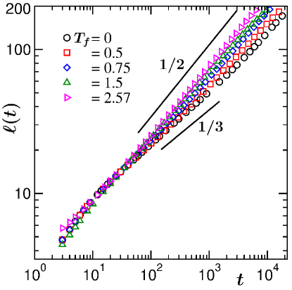
Figure 1: Average domain lengths, $\ell(t)$, are plotted versus time, on a log-log scale. Results from different final temperatures are presented. The solid lines are power-laws. The values of the exponents are mentioned.

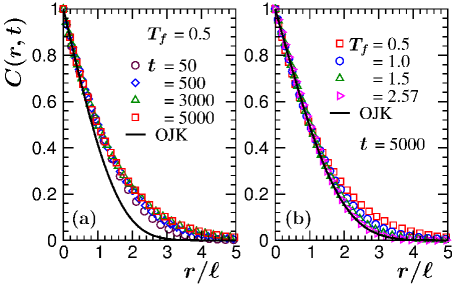
Figure 2: (a) Two-point equal time correlation functions, $C(r,t)$, are plotted versus the scaled distance $r/\ell$, for $T_{f}=0.5$. Data from few different times are shown. (b) Same as (a) but here we have shown $C(r,t)$ from different final temperatures. In each of the cases we have chosen $t=5000$ that fall in the scaling regimes. In both (a) and (b) the continuous lines represent the Ohta-Jasnow-Kawasaki (OJK) function. The correlation functions have been plotted in such a way that there exists good collapse in the early abscissa range.

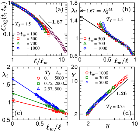
Figure 3: (a) $C_{\textrm{ag}}(t,t_{w})$, the autocorrelation functions, are plotted versus $\ell/\ell_{w}$, on a log-log scale. Data from different $t_{w}$, for $T_{f}=1.5$, are included. The solid line is a power-law with $\lambda=\lambda_{3}^{\rm{LM}}=1.67$. (b) The instantaneous exponents $\lambda_{i}$ are shown as a function of $\ell_{w}/\ell$, for the same final temperature. The arrow-headed line is a linear extrapolation to the $\ell/\ell_{w}=\infty$ limit, done by excluding the late time finite-size affected as well as early time domain-magnetization relaxation parts. (c) Here we have shown $\lambda_{i}$, as a function of $\ell_{w}/\ell$, for a few different values of $T_{f}$. In each of the cases $t_{w}$ belongs to the scaling regime. The arrow-headed lines are linear guides to the eyes. (d) Finite-size scaling plot of $C_{\rm{ag}}(t,t_{w})$ for $T_{f}=0.75$. The solid line there corresponds to a power-law with the value of the exponent mentioned near the line.

In Fig. 2(a) we show plots of $C(r,t)$, from different times, by scaling the distance axis by a characteristic length, extracted by exploiting the satisfaction of scaling of $C(r,t)$ at small distances, for $T_{f}=0.5$. It appears that the collapse starts only from $t\gtrsim 1000$, approximately the time since when departure to $\alpha=1/2$ behavior starts. This general picture is true for other low temperatures also. In Fig. 2(b) we have shown $C(r,t)$, again versus $r/\ell$, from the scaling regimes of different $T_{f}$ values. Interestingly, $\tilde{C}(r/\ell)$ at different $T_{f}$ values do not agree with each other. However, with the increase of $T_{f}$ the agreement with the OJK function $[\tilde{C}_{\rm{OJK}}(r/\ell)]$ ohta keeps getting better. This observation suggests that perhaps there exists a special temperature $T_{\rm{sp}}$ ($<T_{c}$), beyond which the coarsening dynamics is more unique than below it. In fact for $T_{f}=T_{R}$ the agreement between simulation data and the OJK function is quite well. We will return to this central theme after discussion of the basic results on aging.

Fig. 3(a) shows plots of $C_{\textrm{ag}}(t,t_{w})$, with the variation of $\ell/\ell_{w}$. The value of $T_{f}$ for this representative case is set at $1.5$. Data sets from a few different waiting times are shown. Good collapse of data is visible for the considered values of $t_{w}$. However, there exist deviations from the master curve, for $\ell/\ell_{w}>>1$. These are related to finite-size effects das4 . Decay in the finite-size unaffected regime does not appear consistent with the LM value liu – see the disagreement with the solid line. In Fig. 3(b) we show the instantaneous exponent dfisher ; das4 $\lambda_{i}$ $[=-\textrm{d}\ln C_{\textrm{ag}}(t,t_{w})/\textrm{d}\ln(\ell/\ell_{w})]$ as a function of $\ell_{w}/\ell$, for multiple choices of $t_{w}$ lying in the scaling regime. The data sets appear linear in the finite-size unaffected regimes. Note that at early time relaxation of domain magnetization interferes and should be discarded from the process of estimation of $\lambda$. A linear extrapolation to $\ell/\ell_{w}=\infty$ provides $\lambda\simeq 1.5$. Given that the above quoted number lies between $\lambda_{3}^{\rm{LM}}$ and $\lambda(T_{f}=0)$, being significantly different from each of these, one gets a strong hint on the presence of a special point.

In Fig. 3(c) we show plots of $\lambda_{i}$, as a function of $\ell_{w}/\ell$, for few different values of $T_{f}$. Here we discarded the parts corresponding to finite-size effects and equilibration of domain magnetization. Furthermore, in each of the cases the results are from well inside the scaling regimes of $t_{w}$. The arrow-headed lines are related to the estimations of the values of $\lambda$, from linear extrapolations to the $\ell_{w}/\ell=\infty$ limit. Clearly, $\lambda$ depends strongly on $T_{f}$. The accuracy of these estimates is validated by the independent quantifications of $\lambda$ via a finite-size scaling method das4 ; das_pre_fss . A representative exercise related to this is shown in Fig. 3(d), for $T_{f}=0.75$. In this figure $Y$ is a $t_{w}$-independent scaling function and $y$ is a dimensionless scaling variable. Note that here we have avoided studying systems of different sizes, contrary to the standard practice in the literature of such analysis. Instead, we have obtained collapse of data from different $t_{w}$ values. Note that when $t_{w}$ is varied a system has different effective sizes to grow further. Details of the scaling construction is provided below.

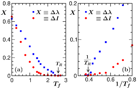
Figure 4: (a) Plots are shown by comparing $\Delta\lambda$ and $\Delta I$ with the variation of $T_{f}$. (b) Plots of $\Delta\lambda$ and $\Delta I$ as a function of $1/T_{f}$. The locations of $T_{R}$ are marked inside the frames.

The behavior of $\lambda_{i}$ in Fig. 3(b) and Fig. 3(c) suggest $\lambda_{i}=\lambda-B/x$, with $x=\ell/\ell_{w}$ and $B$ being a constant, in the finite-size unaffected late time regime. This leads to a form das4 ; das_pre_fss $C_{\textrm{ag}}(t,t_{w})=Ae^{-B/x}x^{-\lambda}$. By taking $y=L/\ell$ as a scaling variable and $y_{w}=L/\ell_{w}$, a finite-size scaling function can be written as das3 $Y=C_{\textrm{ag}}(t,t_{w})e^{By/y_{w}}y_{w}^{\lambda}$, where $Y$ contains a factor $y^{\lambda}$. When results from different $t_{w}$ are plotted, for optimum choices of the unknown parameters, including $\lambda$, there will be collapse of data sets that will satisfy the expected $y^{\lambda}$ behavior at large $y$. This is demonstrated in Fig. 3(d) for $T_{f}=0.75$. Here the collapse is obtained for $\lambda=1.26$, the number being consistent with the value that was suggested by the exercise in Fig. 3(c). Next we quantify the special temperature from a more systematic study.

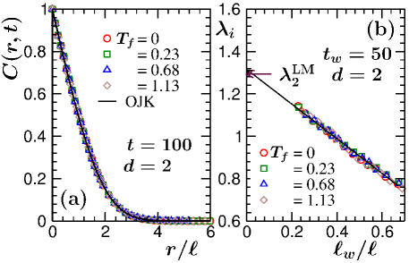
Figure 5: (a) Plots of scaled two-point equal time correlation functions, $C(r,t)$, from $d=2$, for different $T_{f}$ values. The time has been chosen from the scaling regime. The continuous line represents the OJK function. (b) The instantaneous exponents, $\lambda_{i}$, are plotted as a function of $\ell_{w}/\ell$, for different $T_{f}$ values. The solid line is a common linear extrapolation of the data sets. The arrow-headed horizontal line points to the LM value of $\lambda$ in $d=2$.

In Fig. 4(a) we show $\Delta\lambda=\lambda_{3}^{\rm{LM}}-\lambda(T_{f})$, as a function of $T_{f}$. Given that the general expectation is $\lambda_{3}^{\rm{LM}}$, it is meaningful to look at the stated difference. There appears to be a nice convergence of the data set to zero as $T_{f}\rightarrow T_{\rm{R}}\simeq 2.57$. With respect to the deviation of $\tilde{C}(r/\ell)$ from the OJK form ohta , that we observed above, there may also be a similar trend. In this case an appropriate quantity to consider is $\Delta I=\int dr[\tilde{C}(r/\ell)-\tilde{C}_{\rm{OJK}}(r/\ell)]$. Here note that there exists an LM form for $C(r,t)$ as well liu . However, this practically overlaps with the OJK function. It will be interesting to see if $\Delta I$ approaches zero at the same $T_{f}$ as in the case of $\Delta\lambda$. Thus, in Fig. 4(a) we have included the $T_{f}$-dependence of $\Delta I$ as well. The presented data sets are in nice agreement with each other, over a wide range of temperature, within a factor – see Fig. 4(b) for a clearer convergence to zero for $T_{f}\rightarrow T_{R}$.

In Fig. 5 we show analogous results from $d=2$. Fig. 5(a) contains results for the scaled $C(r,t)$ and in Fig. 5(b) we have shown data for $\lambda_{i}$, as a function of $\ell_{w}/\ell$. For each of the cases results from a wide range of $T_{f}$ are included. The anomalies present in $d=3$ are clearly absent in this case. No detectable $T_{f}$-dependence can be observed. The theoretical expectations are satisfied over the whole range of $T_{f}$. Recall that in this dimension, a nonzero roughening transition temperature does not exist for this model.

IV Conclusions

From extensive Monte Carlo simulations landau we have presented results on nonequilibrium dynamics in the Glauber landau ; glauber Ising model. This mimics ordering in uniaxial ferromagnets. Our quantitative analysis of data from space dimension $d=3$ on structure, growth and aging, over a wide range of temperature below the critical point, suggests that the low temperature behavior is anomalous.

We show that that the anomalies are not unique to the case of zero temperature quench, as was previously thought. Various quantities exhibit zero-temperature-like trend till a certain nonzero value of $T_{f}$. Above this temperature, behavior of all the aspects become consistent with various theoretical expectations bray ; liu ; ohta ; allen . This transition or special temperature coincides with that of the roughening transition beijern . Such a conclusion appears more meaningful from the fact that these anomalies are absent in $d=2$ and for this dimension roughening transition temperature is zero.

To understand the anomalies, more detailed theoretical investigations by exploiting the well travelled auxiliary field ansatz should be carried out yeung . Recently, it was shown mpemba_pccp that the ordering dynamics in the Glauber Ising model exhibits Mpemba effect. It needs to be further investigated in light of the present observation.

SKD acknowledges previous collaborations on similar matter with S. Chakraborty, S. Majumder and J. Midya. The authors are grateful to SERB, DST, INDIA for support via Grant No. MTR/2019/001585.

References

- (1) V. Spirin, P.L. Krapivsky, and S. Redner, Phys. Rev. E 63, 036118 (2001).
- (2) V. Spirin, P.L. Krapivsky, and S. Redner, Phys. Rev. E 65, 016119 (2001).
- (3) P.M.C. de Oliveira, C.M. Newman, V. Sidoravicious, and D.L. Stein, J. Phys. A 39, 6841 (2006).
- (4) G. Kondrat and K. Sznajd-Weron, Phys. Rev. E 79, 011119 (2009).
- (5) J.J. Arenzon, A.J. Bray, L.F. Cugliandolo, and A. Sicilia, Phys. Rev. Lett. 98, 145701 (2007).
- (6) J. Olejarz, P.L. Krapivsky, and S. Redner, Phys. Rev. Lett. 109, 195702 (2012).
- (7) J. Olejarz, P.L. Krapivsky, and S. Redner, Phys. Rev. E 83, 051104 (2011).
- (8) J. Olejarz, P.L. Krapivsky, and S. Redner, Phys. Rev. E 83, 030104 (2011).
- (9) F. Corberi, E. Lippiello, and M. Zannetti, Phys. Rev. E 78, 011109 (2008).
- (10) T. Blanchard, F. Corberi, L.F. Cugliandolo, and M. Picco, Europhys. Lett. 106, 66001 (2014).
- (11) T. Blanchard, L.F. Cugliandolo, M. Picco, and A. Tartaglia, J. Stat. Mech. 2017, P113201.
- (12) J.G. Amar and F. Family, Bull. Am. Phys. Soc. 34, 491 (1989).
- (13) J.D. Shore, M. Holzer, and J.P. Sethna, Phys. Rev. B 46, 11376 (1992).
- (14) S. Cueille and C. Sire, J. Phys. A 30, L791 (1997).
- (15) S.K. Das and S. Chakraborty, Eur. Phys. J. Spec. Top. 226, 765 (2017).
- (16) S. Chakraborty and S.K. Das, Europhys. Lett. 119, 50005 (2017).
- (17) N. Vadakkayil, S. Chakraborty and S.K. Das, J. Chem. Phys. 150, 054702 (2019).
- (18) J. Denholm and B. Hourahina, J. Stat. Mech: Theory and Expt. 2020, 093205 (2020).
- (19) C. Godriche and M. Pleimling, J. Stat. Mech 2018, 043209 (2018).
- (20) P. Mullick and P. Sen, Phys. Rev. E 95, 052150 (2017).
- (21) U. Yu, J. Stat. Mech 2017, 123203 (2017).
- (22) L.F. Cugliandolo, Comptes Rendus Physique 16, 257 (2015).
- (23) F. Liu and G.F. Mazenko, Phys. Rev. B 44, 9185 (1991).
- (24) T. Ohta, D. Jasnow, and K. Kawasaki, Phys. Rev. Lett. 49, 1223 (1982).
- (25) C. Yeung, Phys. Rev. Lett. 61, 1135 (1988).
- (26) M.E. Fisher, Rep. Prog. Phys. 30, 615 (1967).
- (27) H. Van Beijern and I. Nolden, in Structure and Dynamics of Surfaces II: Phenomena, Models and Methods, Topics in Current Physics, vol. 43, ed. W. Schommers and P. von Blanckenhagen (Springer, Berlin, 1987).
- (28) A.J. Bray, Adv. Phys. 51, 481 (2002).
- (29) S. Puri and V. Wadhawan (ed.), Kinetics of Phase Transitions (CRC Press, Boca Raton, 2009).
- (30) D.S. Fisher and D.A. Huse, Phys. Rev. B 38, 373 (1988).
- (31) C. Yeung, M. Rao, and R.C. Desai, Phys. Rev. E 53, 3073 (1996).
- (32) M. Henkel, A. Picone, and M. Pleimling, Europhys. Lett. 68, 191 (2004).
- (33) E. Lorenz and W. Janke, Europhys. Lett. 77, 10003 (2007).
- (34) J. Midya, S. Majumder, and S.K. Das, J. Phys.: Condens. Matter 26, 452202 (2014).
- (35) D.A. Huse, Phys. Rev. B 34, 7845 (1986).
- (36) S. Majumder and S.K. Das, Phys. Rev. E 84, 021110 (2011).
- (37) S.M. Allen and J.W. Cahn, Acta Metall. 27, 1085 (1979).
- (38) D.P. Landau and K. Binder, A Guide to Monte Carlo Simulations in Statistical Physics (Cambridge University Press, Cambridge, 2009).
- (39) J. Midya and S.K. Das, Phys. Rev. Lett. 118, 165701 (2017).
- (40) M.E. Fisher and M.N. Barber, Phys. Rev. Lett. 28, 1516 (1972).
- (41) J. Midya, S. Majumder, and S.K. Das, Phys. Rev. E 92, 022124 (2015).
- (42) R.J. Glauber, J. Math. Phys. 4, 294 (1963).
- (43) C. Yeung, Phys. Rev. E 97, 062107 (2018).
- (44) N. Vadakkayil and S.K. Das, Phys. Chem. Chem. Phys 23, 11186 (2021).