Abstract

We revisit the theoretical properties of Hamiltonian stochastic differential equations (sdes) for Bayesian posterior sampling, and we study the two types of errors that arise from numerical sde simulation: the discretization error and the error due to noisy gradient estimates in the context of data subsampling. Our main result is a novel analysis for the effect of mini-batches through the lens of differential operator splitting, revising previous literature results. The stochastic component of a Hamiltonian sde is decoupled from the gradient noise, for which we make no normality assumptions. This leads to the identification of a convergence bottleneck: when considering mini-batches, the best achievable error rate is $\mathcal{O}(\eta^{2})$, with $\eta$ being the integrator step size. Our theoretical results are supported by an empirical study on a variety of regression and classification tasks for Bayesian neural networks.

1 INTRODUCTION

Hamiltonian Monte Carlo (hmc) is a popular approach to obtain samples from intractable distributions (Neal, 1996; Neal et al., 2011; Hoffman and Gelman, 2014). It presents, however, significant computational challenges for large datasets, as it requires access to the full gradient of the associated Hamiltonian system. Stochastic-Gradient hmc (sghmc) (Chen et al., 2014) was proposed as a scalable alternative to hmc, by admitting noisy estimates of the gradient using mini-batching. In sghmc, the Hamiltonian dynamics is modified so as to include a friction term that counteracts the effects of the gradient noise. This approach has proven effective in dealing with the difficulties in sampling from the posterior distribution over model parameters of Bayesian Neural/Convolutional Networks (bnns) (Wenzel et al., 2020; Tran et al., 2020).

Stochastic gradient (sg) methods have been extensively studied as a means for Markov chain Monte Carlo (mcmc)-based algorithms to scale to large data. Variants of sg-mcmc algorithms have been studied through the lenses of first (Welling and Teh, 2011; Ahn et al., 2012; Patterson and Teh, 2013) or second-order (Chen et al., 2014; Ma et al., 2015) Langevin dynamics; these are mathematically convenient continuous-time processes which correspond to discrete-time gradient methods with and without momentum, respectively. Langevin dynamics are formally captured by an appropriate set of stochastic differential equations (sdes), whose theoretical properties have been extensively studied (Kloeden and Platen, 2013; Debussche and Faou, 2012) with a particular emphasis on the stationary property of these processes (Abdulle et al., 2014; Milstein and Tretyakov, 2007). As in Abdulle et al. (2014, 2015), we are interested in the asymptotic (in time) performance of such sampling schemes. The reader is referred to Vollmer et al. (2016); Gao et al. (2018b, a); Futami et al. (2020); Xu et al. (2018) for additional insights into the non-asymptotic behavior of these methods.

In this work, we seek to re-evaluate the connections between sg and stochastic Hamiltonian dynamics (also known as second order or underdamped Langevin dynamics) with the aim of improving our current understanding of the goodness of sampling from intractable distributions when considering mini-batching. We consider a system with potential $U(\boldsymbol{\theta})$ which is the negative of the logarithm of the density function associated with the distribution we aim to sample from. We then introduce position variables $\boldsymbol{\theta}\in\mathbb{R}^{d}$ (i.e., parameters) and momentum variables $\mathbf{r}\in\mathbb{R}^{d}$ obeying the following sde:

$$\begin{split}d\mathbf{r}(t)&=-\nabla_{\boldsymbol{\theta}}U(\boldsymbol{\theta}(t))dt-C\mathbf{M}^{-1}\mathbf{r}(t)dt+\sqrt{2C}d\mathbf{w}(t)\\ d\boldsymbol{\theta}(t)&=\mathbf{M}^{-1}\mathbf{r}(t)dt.\end{split}$$ (1)

This is an extension of an Hamiltonian system with a friction term and an appropriately scaled Brownian motion $\mathbf{w}(t)$, where $C>0$ and $\mathbf{M}$ is a symmetric, positive definite matrix (a.k.a. mass matrix). A common assumption in the literature (Chen et al., 2014; Ahn et al., 2012; Ma et al., 2015), is that the noise associated with stochastic estimates of $\nabla_{\boldsymbol{\theta}}U(\boldsymbol{\theta}(t))$ is normally distributed. This noise is linked with the additive Brownian motion term in Eq. 1.

In this work we challenge this assumption and we advocate that sg should be completely decoupled from the sde dynamics. More specifically, we show that the Brownian motion term is not a good model for the stochasticity of the gradient introduced by the mini-batching scheme (see also Appendix A for an extended discussion). In this sense, our framework is similar to Chen et al. (2015); however we propose an interpretation of the effect of mini-batching through the lenses of differential operator splitting, by leveraging the huge literature concerning the simulation of high dimensional Hamiltonian systems (Childs et al., 2021; Suzuki, 1977; Hatano and Suzuki, 2005; Childs and Su, 2019; Low et al., 2019). Earlier attempts (Betancourt, 2015; Shahbaba et al., 2014) to use operator splitting as a tool to describe mini-batching focus on hmc, whereas Hamiltonian sde dynamics have never been studied under this formalism, to the best of our knowledge. Recently Zou and Gu (2021) have studied non-asymptotic convergence for hmc when considering mini-batches, but these results are limited to strongly convex potentials.

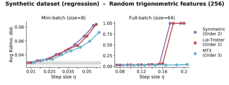
Figure 1: We evaluate integrators of different orders based on the distance from the true posterior distribution for a Gaussian-linear system. Left: for mini-batch size equal to $8$, there is an area for which the 3-rd order integrator does not perform any better than integrators of lower order. Right: There is no such bottleneck for the full-batch version.

Our main contribution can be summarized as the derivation of new convergence results considering the two types of error induced by the simulation of the proposed sde scheme: the discretization and the sg errors. The discretization of sdes has been extensively studied in the literature (Kloeden and Platen, 2013; Debussche and Faou, 2012; Abdulle et al., 2014; Milstein and Tretyakov, 2007). In Section 2, we leverage these results to present quantitatively precise claims about sampling schemes in the context of Bayesian inference for modern machine learning problems. In Section 3, our treatment of mini-batches in terms of differential operator splitting does not rely on Gaussian assumptions regarding the form of the noise. Given a numerical integrator of order $p$ and step size $\eta$, we show that although the discretization error vanishes at a rate $O(\eta^{p})$, the sg error vanishes at rate $O(\eta^{2})$. We thus identify a convergence bottleneck, as demonstrated on an example (details in Section F.1) in Figure 1, introduced by the mini-batching. This result is in contrast with the current understanding of convergence properties of sampling algorithms (Chen et al., 2015). Our work then updates the previous best result about convergence rates for a broad range of integrators and with minimal assumptions about the mini-batching process.

Our second contribution (Section 4) is a reinterpretation of the hmc algorithm with partial momentum refreshment (Neal et al., 2011; Horowitz, 1991) as an integrator for Hamiltonian sdes (Abdulle et al., 2015). This connection provides insights into the behavior of classical hmc schemes and extends the results of our theoretical analysis.

In Section 5, we conduct an extensive experimental campaign that corroborates our theory on the convergence rate of various Hamiltonian-based sde schemes, by exploring the behavior of step size and mini-batch size for a large number of models and datasets.

2 HAMILTONIAN SDES FOR SAMPLING

Given a dataset of observations $\mathrm{D}=\{\mathbf{x}_{i}\}_{i=1}^{N}$, the Bayesian treatment of machine learning models can be summarized as the combination of a prior belief $p(\boldsymbol{\theta})$ and a likelihood function $p(\mathrm{D}|\boldsymbol{\theta})$, into a posterior distribution $p(\boldsymbol{\theta}|\mathrm{D})\propto p(\mathrm{D}|\boldsymbol{\theta})p(\boldsymbol{\theta})$. Since the posterior is analytically intractable for non-linear models such as bnns (Bishop, 2006), our goal is to draw samples from the density $p(\boldsymbol{\theta}|\mathrm{D})$, which is expressed implicitly in exponential form as $p(\boldsymbol{\theta}|\mathrm{D})\propto\exp(-U(\boldsymbol{\theta}))$, where:

$$-U(\boldsymbol{\theta})=\sum\limits_{i=1}^{N}\log p(\mathbf{x}_{i}|\boldsymbol{\theta})+\log p(\boldsymbol{\theta}),\qquad$$

$$\text{and}\qquad p(\mathrm{D}|\boldsymbol{\theta})=\prod_{i=1}^{N}p(\mathbf{x}_{i}|\boldsymbol{\theta}).$$ (2)

In Hamiltonian systems, $U(\boldsymbol{\theta})$ is known as the potential, which, together with a kinetic energy term, yields the Hamiltonian function $H(\mathbf{z})=U(\boldsymbol{\theta})+\nicefrac{{1}}{{2}}||\mathbf{M}^{-1}\mathbf{r}||^{2}$. The vector $\mathbf{z}=[\mathbf{r}^{\top},\boldsymbol{\theta}^{\top}]^{\top}$ denotes the overall system state, which includes the position $\boldsymbol{\theta}$ (i.e., parameters) and the conjugate momentum $\mathbf{r}$, while $\mathbf{M}$ is a symmetric, positive definite mass matrix. Then, we consider the following sde, which is a compact form of Eq. 1:

$$d\mathbf{z}(t)=\begin{bmatrix}-C\boldsymbol{I}&-\boldsymbol{I}\\ \boldsymbol{I}&\mathbf{0}\end{bmatrix}\nabla H(\mathbf{z}(t))dt+\begin{bmatrix}\sqrt{2C}d\mathbf{w}(t)\\ \mathbf{0}\end{bmatrix}.$$ (3)

We study the stationary behavior of the process of Eq. 3, defining $\nabla_{\mathbf{z}}=[\nabla_{\mathbf{r}}^{\top},\nabla_{\boldsymbol{\theta}}^{\top}]^{\top}$, through the following differential operator:

$$\mathcal{L}=-\left(\nabla^{\top}_{\boldsymbol{\theta}}U(\boldsymbol{\theta})\right)\nabla_{\mathbf{r}}+\left(\left(\mathbf{M}^{-1}\mathbf{r}\right)^{\top}\right)\nabla_{\boldsymbol{\theta}}$$

$$-C\left(\left(\mathbf{M}^{-1}\mathbf{r}\right)^{\top}\right)\nabla_{\mathbf{r}}+C\nabla_{\mathbf{r}}^{\top}\nabla_{\mathbf{r}},$$ (4)

which is known as the infinitesimal generator. The Fokker Planck equation, that can be used to obtain the stationary distribution $\rho_{ss}(\mathbf{z})$ of the stochastic process writes as $\mathcal{L}^{\dagger}\rho_{ss}=0$, where ^† indicates the adjoint of the operator. Some sample paths for a simple two-parameter logistic regression can be seen in Fig. 2, where we vary the constant $C$. Although the stationary distribution is independent of $C$, the transient dynamics change, resulting in paths of different form, as we see in the figure. Essentially, $C$ is a user-defined parameter whose effect we explore in Section F.4 for a wide range of machine learning models. Then we have the following theorem:

Theorem 1.

For an ergodic stochastic process described by the sde of Eq. 3 with stationary distribution $\rho_{ss}(\mathbf{z})$ we have:

$$\rho_{ss}(\mathbf{z})\propto\exp(-H(\mathbf{z}))=\exp(-U(\boldsymbol{\theta})-\nicefrac{{1}}{{2}}||\mathbf{M}^{-1}\mathbf{r}||^{2})$$ (5)

The proof can be found in Section B.2. A direct implication is that simulating the stochastic process allows us to compute ergodic averages of functions of interest $\phi(\mathbf{z})$, of the form $\int\phi(\mathbf{z})\rho_{ss}(\mathbf{z})d\mathbf{z}$ (details in Appendix B). Since $\rho_{ss}(\mathbf{z})=\rho_{ss}(\boldsymbol{\theta})\rho_{ss}(\mathbf{r})$, the procedure can be used to perform Bayesian averages of functions of $\boldsymbol{\theta}$ only, $\phi(\boldsymbol{\theta})$ , as the following holds $\int\phi(\boldsymbol{\theta})p(\boldsymbol{\theta}|\mathrm{D})d\boldsymbol{\theta}=\int\phi(\boldsymbol{\theta})\rho_{ss}(\boldsymbol{\theta})d\boldsymbol{\theta}$. In this paper the theoretical derivations are carried out for generic functions of $\mathbf{z}$.

We shall refer to our scheme as sde-based hmc (shmc). This is different from sghmc, for which Eq. 3 is modified so that the Brownian motion term has covariance $2(\mathbf{C}-\tilde{\mathbf{V}})$, where $\tilde{\mathbf{V}}$ is an estimate of the covariance of the gradient. This was done to counterbalance the effect of the stochastic gradient, which we believe is not necessary, as we discuss in Section 5.

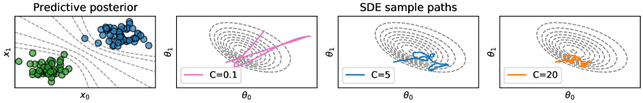
Figure 2: Sample paths for simple a two-parameter logistic regression problem (shown in the leftmost panel). We show sde paths for different choices of friction coefficient $C$.

Remark: In recent literature, Eq. 3 has been associated with normally-distributed estimates of the gradient (Chen et al., 2014; Mandt et al., 2017). In our view, however, this connection is not well-justified, as for the Brownian motion term of Eq. 3 we have that $d\mathbf{w}(t)=\sqrt{dt}\mathcal{N}(\mathbf{0},\boldsymbol{I})$, while a (Gaussian) stochastic gradient term in the continuous limit becomes $dt\mathcal{N}(\mathbf{0},\boldsymbol{I})$. A more detailed exposition can be found in Appendix A. Our alternative treatment for the study of the effect of mini-batches follows in Section 3.

2.1 Ergodic errors of sdes

Except from a handful of cases, it is not possible to draw exact sample paths from arbitrary sdes. We consider a generic numerical integrator $\psi$, with step size $\eta$, whose purpose is to simulate the stochastic evolution of the sde of interest. Formally, we look for a stochastic mapping, that from a given initial condition $\mathbf{z}_{0}$, generates a new random variable $\mathbf{z}_{1}=\psi(\mathbf{z}_{0};\eta)$ by faithfully simulating the true continuous time stochastic dynamics $\mathbf{z}(\eta)|_{\mathbf{z}(0)=\mathbf{z}_{0}}$. Several quantitative metrics measuring the degree of accuracy of the simulation are available (Kloeden and Platen, 2013). The simplest is the strong error, which is the expected difference between true paths and simulated ones. Relaxing to the expected difference between functions of paths corresponds to quantifying the weak error:

Definition 1.

(Debussche and Faou, 2012) Consider Eq. 3 with initial condition $\mathbf{z}_{0}$. The numerical integrator $\psi$ has weak order of convergence $p$ if $|\mathbb{E}\left[\phi(\psi(\mathbf{z}_{0};\eta))\right]-\mathbb{E}\left[\phi(\mathbf{z}(\eta))\right]|=\mathcal{O}(\eta^{p+1})$, where $\mathbf{z}(\eta)$ is the value taken by Eq. 3 after a time $\eta$, the chosen step size.

The transformation of the functions $\phi(\mathbf{z})$ of the true stochastic dynamics $\mathbf{z}(t)$, starting from initial conditions $\mathbf{z}_{0}$ is described by the Kolmogorov differential equation $\mathbb{E}\left[\phi(\mathbf{z}(t))\right]=\exp{(t\mathcal{L})}\phi(\mathbf{z})|_{\mathbf{z}=\mathbf{z}_{0}}$, that throughout the paper we indicate with abuse of notation as $\mathbb{E}\left[\phi(\mathbf{z}(t))\right]=\exp{(t\mathcal{L})}\phi(\mathbf{z}_{0})$. The operator $\mathcal{U}$, defined as $\mathcal{U}\phi(\mathbf{z}_{0})=\mathbb{E}\left[\phi(\psi(\mathbf{z}_{0};\eta))\right]$, represents a $p_{\text{th}}$ order weak integrator if $\mathcal{U}=\exp{(\eta\mathcal{L})}+\mathcal{O}(\eta^{p+1})$.

Since we are only interested in samples from $p(\boldsymbol{\theta}|D)$, it is sufficient to consider the even weaker ergodic average error, defined hereafter. The numerical integrator iteratively induces a stochastic process $\mathbf{z}_{i}=\psi({\mathbf{z}_{i-1}};\eta),i=1,\dots N$. The ergodic average of a given function $\phi(\cdot)$ converges to the integral $\int\phi(\mathbf{z})\rho^{\psi}_{ss}(\mathbf{z})d\mathbf{z}$, where $\rho^{\psi}_{ss}$ is the stationary distribution of the stochastic process induced by the numerical integrator $\psi$. The ergodic average error is the difference between the ergodic average of the numerical integrator and the true average obtained with the stationary distribution of Eq. 3:

$$e(\psi,\phi)=\int\phi(\mathbf{z})\rho^{\psi}_{ss}(\mathbf{z})d\mathbf{z}-\int\phi(\mathbf{z})\rho_{ss}(\mathbf{z})d\mathbf{z}.$$ (6)

We stress that, although outside the scope of this work, the results presented here can be extended to non-asymptotic (in time) settings. Indeed the error with respect to a finite time empirical average can be expressed as $\frac{1}{N}\sum\limits_{n=0}^{N-1}\phi(\mathbf{z}_{n})-\int\phi(\mathbf{z})\rho_{ss}(\mathbf{z})d\mathbf{z}$. By triangle inequality its absolute value can be bounded by $|\frac{1}{N}\sum\limits_{n=0}^{N-1}\phi(\mathbf{z}_{n})-\int\phi(\mathbf{z})\rho^{\psi}_{ss}(\mathbf{z})d\mathbf{z}|+|e(\psi,\phi)||$. The first term can be bounded in expectation by considering the convergence speed (as a function of time) to the stationary distribution of the numerical integration scheme, either by classical arguments or attempting a weak backward error analysis characterization (Debussche and Faou, 2012). In this work we consider only the quantity in Eq. 6.

Our goal is to characterize the rate of convergence to zero for $e(\psi,\phi)$ as a function of the step size $\eta$, the most important free parameter. A sufficient condition for an integrator to be of a given ergodic order $p$, i.e. $e(\psi,\phi)=\mathcal{O}(\eta^{p})$, is to have weak order $p$ (Abdulle et al., 2014). See Section B.3 for a more detailed exposition.

2.2 Numerical integrators

We explore the effect of a number of sde integrators of weak order two and three; these schemes are outlined in detail in Section B.5. Hamiltonian systems evolve on manifolds with peculiar geometrical properties whose study is the subject of symplectic geometry. In Section B.4 we present the class of quasi-symplectic integrators (Milstein and Tretyakov, 2003). For the purpose of understanding the main text it is sufficient to know that such integrators are empirically known to outperform their non-symplectic counterpart.

The leapfrog scheme is probably the simplest form of quasi-symplectic integrator, which involves updating the position and momentum at interleaved time steps. Importantly, while it has theoretically order-one of convergence both in weak and ergodic sense, we observe empirically that its performance is very close to other quasi-symplectic order-two schemes. A similar phenomenon has been observed by Milstein and Tretyakov (2003).

In the experimental section, we also examine the symmetric splitting integrator proposed in Chen et al. (2015) (symmetric), which is also compatible with our shmc scheme. Finally we consider a lie-trotter splitting scheme (Abdulle et al., 2015) that is of weak order-two, while it is also quasi-symplectic. In Section 4 this scheme will be used to draw a theoretical connection between hmc (Neal et al., 2011) and the proposed sde framework in Eq. 3.

In order to demonstrate the convergence bottleneck more clearly, we also include an integrator of third order in our comparisons. We employ the 3-stage quasi-symplectic integrator of Milstein and Tretyakov (2003). This scheme might not be always practical, as it involves three stages and one computation of the Hessian. However, it is sufficient to demonstrate the convergence bottleneck effect due to mini-batches.

3 MINIBATCHES AS OPERATOR SPLITTING

Traditionally, the effect of mini-batching has been modeled as a source of additional independent Gaussian noise (Chen et al., 2014) at every step of the simulated dynamics. We challenge this common modeling assumption by considering the geometrical perspective of differential operator splitting. We build the link between the true generator $\mathcal{L}$ and numerical integration performed using mini-batch subsets of the full potential. Our analysis does not make any assumption about Gaussianity of sg noise. Our approach is rooted in the geometrical view of splitting schemes for high dimensional Hamiltonian systems (Childs et al., 2021; Suzuki, 1977; Hatano and Suzuki, 2005; Childs and Su, 2019; Low et al., 2019). This allows us to derive Theorem 3, which presents a result in terms of convergence rate to the desired posterior distribution. A purely geometrical approach has not received much attention in the context of data subsampling for Bayesian inference, with the notable exceptions of Betancourt (2015); Shahbaba et al. (2014) that explored related ideas for the case of hmc only.

Without loss of generality, suppose that the dataset $\mathrm{D}$ is split into two mini-batches $\mathrm{D}_{1},\mathrm{D}_{2}$. Following Eq. 4 we can define the infinitesimal generators $\mathcal{L}_{1},\mathcal{L}_{2}$, for which we have $\mathcal{L}=\mathcal{L}_{1}+\mathcal{L}_{2}$. Intuitively, given an operator in exponential form $\exp(\eta(\mathcal{L}_{1}+\mathcal{L}_{2}))$, we would like to determine under which conditions the following holds

$$\exp(\eta(\mathcal{L}_{1}+\mathcal{L}_{2}))\simeq\exp(\eta\mathcal{L}_{1})\exp(\eta\mathcal{L}_{2}),$$ (7)

and to quantify the discrepancy error in a rigorous way. In the general case we consider splitting $\mathcal{L}$ into $K$ mini-batches of the form $\mathcal{L}=\sum\limits_{i=1}^{K}\mathcal{L}_{i}$ where

$$\mathcal{L}_{i}=-\left(\nabla^{\top}_{\boldsymbol{\theta}}U_{i}(\boldsymbol{\theta})\right)\nabla_{\mathbf{r}}+K^{-1}\left(\left(\mathbf{M}^{-1}\mathbf{r}\right)^{\top}\right)\nabla_{\boldsymbol{\theta}}$$

$$-K^{-1}C\left(\left(\mathbf{M}^{-1}\mathbf{r}\right)^{\top}\right)\nabla_{\mathbf{r}}+K^{-1}C\nabla_{\mathbf{r}}^{\top}\nabla_{\mathbf{r}},$$ (8)

with $U_{i}(\boldsymbol{\theta})$ the potential computed using only the $i_{\text{th}}$ mini-batch. The theorems presented in this section clarify how concatenations of the form $\prod_{i}\exp(\eta K\mathcal{L}_{i})$ induce errors and clarify their relevance for the considered problem.

The following theorem characterizes the order of convergence of the randomized splitting scheme.

Theorem 2.

Split the full dataset into $K$ mini-batches and consider numerical integrators $\psi_{i}$ of order $p$ obtained using the mini-batches, i.e. $\mathbb{E}\left[\phi_{i}(\psi(\mathbf{z}_{0};\eta))\right]=\exp(\eta K\mathcal{L}_{i})\phi(\mathbf{z}_{0})+\mathcal{O}(\eta^{p+1})$. Extract uniformly $\boldsymbol{\pi}=\begin{bmatrix}\pi_{1},\dots,\pi_{K}\end{bmatrix}\in\mathbb{P}$, the set of all the possible permutations of the indeces $\{1,K\}$. The scheme in which initial condition has stochastic evolution through the chain of integrators with order

$$\mathbf{z}_{fin}=\psi_{\pi_{K}}(\psi_{\pi_{K-1}}(\dots\psi_{\pi_{1}}(\mathbf{z}_{0}))),$$ (9)

transforms the functions $\phi$ with an operator $\mathcal{U}$ that has the following expression

$$\mathcal{U}=\exp(\eta K\mathcal{L})+\mathcal{O}(K\eta^{p+1})+\mathcal{O}(K\eta^{3})$$ (10)

The proof can be found in Section C.4. Particularly relevant to our discussion are works that explore randomized splitting schemes for Hamiltonian simulation, but not in a sampling context (Childs et al., 2019; Zhang, 2012).

Theorem 3.

Consider the settings described by Theorem 2. Repeatedly apply the numerical integration scheme. Then the ergodic error has expansion

$$e(\psi,\phi)=\mathcal{O}(\eta^{\min{(p,2)}})$$ (11)

See Section C.5 for the proof. This theorem tells us that the effect of mini-batches is an extra error of order two in the convergence rate. This extra error is not due to an equivalent noise injection into the sde dynamics, and attempting to counterbalance it, as suggested by the literature (Chen et al., 2014), is irrelevant as we will show in Section 5. Importantly, this error can become the bottleneck whenever $p>2$.

The experimental validation carried out in this work, of which Fig. 1 is a prototypical example, confirms the presence of this bottleneck. We include a toy example taken from Vollmer et al. (2016), where an analytical solution is available. The complete specification can be found in Appendix E. The results, reported in Fig. 6, are obtained by comparing an order-2 integrator against an analytical solution, when considering or not mini-batches. Qualitatively, the presence of a bottleneck is clear: when considering mini-batches, the stationary distribution is not the desired one, even with a perfect integrator.

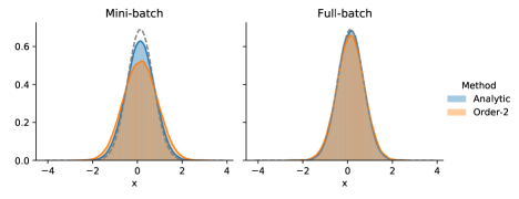
Figure 3: Histograms of stationary distributions. The grey dotted line denotes the true posterior density. Irrespectively of order, mini-batching prevents from convergence to true posterior.

Our main result, the presence of a bottleneck, is in direct disagreement with previous results presented in Chen et al. (2015), where the mini-batching does not affect the ergodic average error. Instead, our theoretical and empirical discussions clearly show that the introduction of mini-batches impedes convergence to the desired posterior.

Details on the constants in the convergence results. Some clarifications are in order. First, the constants in the $\mathcal{O}$ notation of weak and ergodic errors, could be refined considering the geometry of the potentials and the norms inequality of differential operators. We leave such a possibility for future works and refer the interested reader to Childs et al. (2021, 2019) and in particular also to Zhang (2012), that proposes randomized schemes strictly related to the one discussed here. Second, we stress that when performing sampling for Bayesian inference problems, the full potential is divided into mini-batches, and each subset rescaled by the constant $K$. This rescaling allows one to “cover” the same amount of distance per steps independently from $K$, given that with a pure splitting one would need $K$ steps to simulate $\exp(\eta\mathcal{L})$.

For the case of hmc, this connection is acknowledged in Betancourt (2015), drawing an equivalence with the work of Shahbaba et al. (2014).

4 A LIE-TROTTER INTEGRATION SCHEME AND CONNECTIONS WITH HMC

We discuss a sde integration scheme that relies on a lie-trotter splitting of the infinitesimal generator $\mathcal{L}$. That allows us to draw a connection between Hamiltonian sdes and the original hmc family of algorithms, by showing that the latter can be interpreted as an integration scheme of the sde dynamics.

The infinitesimal generator in Eq. 4 can be expressed as the sum $\mathcal{L}=\mathcal{H}+\mathcal{D}$, where:

$$\mathcal{H}=-\left(\nabla^{\top}_{\boldsymbol{\theta}}U(\boldsymbol{\theta})\right)\nabla_{\mathbf{r}}+\left(\left(\mathbf{M}^{-1}\mathbf{r}\right)^{\top}\right)\nabla_{\boldsymbol{\theta}},$$

$$\mathcal{D}=-C\left(\left(\mathbf{M}^{-1}\mathbf{r}\right)^{\top}\right)\nabla_{\mathbf{r}}+C\nabla_{\mathbf{r}}^{\top}\nabla_{\mathbf{r}}.$$

In its general form (Abdulle et al., 2015), the lie-trotter scheme is derived as an application of the Baker–Campbell–Hausdorff formula (Dynkin, 1947), where the dynamics are approximated as follows:

$$\exp(\eta\mathcal{L})=\exp(\nicefrac{{\eta}}{{2}}\mathcal{D})\exp(\eta\mathcal{H})\exp(\nicefrac{{\eta}}{{2}}\mathcal{D})+\mathcal{O}(\eta^{3})$$

In practice, the scheme consists of alternating steps that solve the $\mathcal{H}$ and $\mathcal{D}$ parts of $\mathcal{L}$. The design space is the one of deterministic integrators for the Hamiltonian part $\mathcal{H}$, as the term $\mathcal{D}$ can be solved exactly. Having chosen a deterministic integrator $\psi$, a single step of the sde simulation has the following form:

$$\mathbf{z}^{*}=\begin{bmatrix}{\mathbf{r}^{*}}^{\top},{\boldsymbol{\theta}^{*}}^{\top}\end{bmatrix}^{\top}=\psi(\mathbf{z}_{0}),$$ (12)

$$\mathbf{z}_{1}=\begin{bmatrix}{\exp(-\eta C){\mathbf{r}^{*}}^{\top}+\sqrt{1-\exp(-2\eta C)}\mathbf{w}^{\top},\boldsymbol{\theta}^{*}}^{\top}\end{bmatrix}$$ (13)

It can be shown (Abdulle et al., 2015) that whenever the numerical integrator $\psi$ for the Hamiltonian part $\mathcal{H}$ has order $p$, i.e. $\mathcal{U}\phi=\exp(\eta\mathcal{H})+\mathcal{O}(\eta^{p+1})$, the lie-trotter scheme has convergence order $\mathcal{O}(\eta^{p})$.

In the experiments of Section 5, we consider $\psi$ to be the deterministic version of leapfrog, for which we have $p=2$. Therefore, our practical application of lie-trotter is of order $\mathcal{O}(\eta^{2})$.

hmc with partial momentum refreshment

We examine a generalized hmc variant featuring partial momentum refreshment (Horowitz, 1991; Neal et al., 2011), which consists of two (repeated) steps. First, we have a numerical approximation of a Hamiltonian system by means of a (deterministic) integrator $\psi$:

$$\mathbf{z}^{*}=\begin{bmatrix}{\mathbf{r}^{*}}^{\top},{\boldsymbol{\theta}^{*}}^{\top}\end{bmatrix}^{\top}=\underbrace{\psi(\dots\psi(\psi(}_{N_{l}\text{times}}\mathbf{z}_{0}))),$$ (14)

where $N_{l}$ denotes the number of integration steps and it is assumed to be finite. Then, we have a a partial momentum update as follows:

$$\mathbf{z}_{1}=\begin{bmatrix}{\alpha{\mathbf{r}^{*}}^{\top}+\sqrt{1-\alpha^{2}}\mathbf{w}^{\top},\boldsymbol{\theta}^{*}}^{\top}\end{bmatrix},$$ (15)

where $\mathbf{w}\sim\mathcal{N}(\mathbf{0},\mathbf{I})$ and $\alpha>0$.

The connection between hmc and the lie-trotter is drawn by noticing that mechanically, the two schemes simulate sdes (and thus transform functions) in a similar fashion. lie-trotter transforms functions after a step as $\mathbb{E}\left[\phi(\mathbf{z}_{1})\right]=\mathcal{U}\exp(\eta\mathcal{D})$, while hmc as $\mathbb{E}\left[\phi(\mathbf{z}_{1})\right]=\left(\mathcal{U}\right)^{N_{l}}\exp(\eta N_{l}\mathcal{D})$. The claim is true when we consider the $\alpha$ of hmc to be $\alpha=\exp(-\eta N_{l}C)$ (the full momentum resampling corresponds to $C\rightarrow\infty$).

By exploiting this connection to classical sde integrators, we can thus study the ergodic error of hmc scheme with and without mini-batches. The ergodic error for the two cases is $\mathcal{O}(\eta^{p})$ and $\mathcal{O}(\eta^{\min(p,2)})$ respectively, showing again the bottleneck introduced by mini-batches. See Appendix D for the derivation details.

In both cases, the orders of convergence are independent on $N_{l}$. This is reflected in the experimental results in Section 5. We note that, in practice, the approximation quality degrades by increasing $N_{l}$ for higher learning rates.

5 EXPERIMENTS

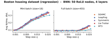
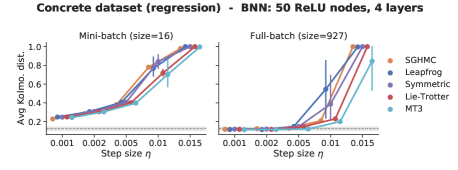
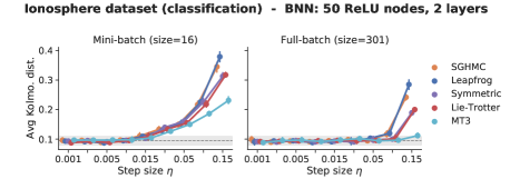
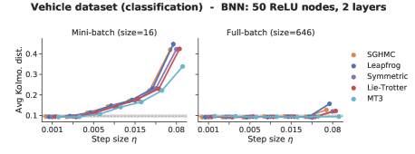
Figure 4: Exploration of step size and batch size for different Hamiltonian-based methods; the grey dotted line denotes the self-distance for the distribution of the oracle.

Comparison framework. The main objective of the experiments is to investigate convergence to the true posterior distribution for a wide range of bnn models and datasets. Metrics that reflect regression and classification accuracy are not of main interest; nevertheless, some of these are reported in Section F.1. Instead, we turn our attention to the quality of the predictive distribution.

We consider the true predictive posterior as the ground truth, which is approximated by a careful application of sghmc (Springenberg et al., 2016) featuring a very small step size and full-batch gradient calculation; this is referred to as the oracle. Any comparison between high-dimensional empirical distributions gives rise to significant challenges. Therefore, we resort to comparing one-dimensional predictive distributions by means of the Kolmogorov distance. For a given test dataset, we explore the average Kolmogorov distance from the true posterior predictive distributions for different methods, step sizes and mini-batch sizes. These should be compared with average Kolmogorov self-distance for the oracle, which is marked as grey dotted lines in the figures that follow. In all cases we compare empirical distributions of 200 samples; the example of Fig. 1 is an exception, where we compare distributions of 2000 samples. See Section F.2 for a complete account.

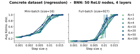
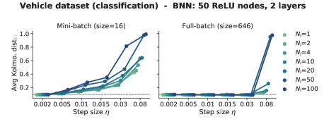
Figure 5: Generalized lie-trotter scheme: Exploration of step size and batch size for different values of the (deterministic) integration length $N_{l}$. The grey dotted line denotes the self-distance for the distribution of the oracle.

For shmc, we examine integrators of different orders: leapfrog, lie-trotter and mt3, and we investigate whether they differ from sghmc (Chen et al., 2014). The leapfrog scheme, which is provably of order 1 for sdes, is also used in sghmc. The lie-trotter integrator introduced in Section 4 is of order 2, while mt3 denotes the order-3 quasi-symplectic integrator of Milstein & Tretyakov (Milstein and Tretyakov, 2003). We also compare against the symmetric splitting integrator proposed in Chen et al. (2015), which we refer to as symmetric. In all cases we set $C=5$; we find this to be a reasonable choice, as can be seen in the exploration of Section F.4.

We consider four regression datasets (boston, concrete, energy, yacht) and two classification datasets (ionosphere, vehicle) from the UCI repository, as well as a 1-D synthetic dataset, for which the regression result is shown in Section F.1. Due to space limitations, here we only present a summary of the results in Figs. 4 and 5. A more detailed exposition, including a more fine-grained exploration of the batch size, can be found in Section F.3 and Section F.4. In what follows, we summarize some findings that apply to all the datasets and models we have considered.

Comparing with sghmc. In Fig. 4 we focus our attention on the comparison between shmc (with leapfrog integrator) and sghmc (Chen et al., 2014). We note that shmc (leapfrog) is different from sghmc in the sense that no counterbalancing of the noise is performed. Nevertheless, we do not observe significant difference between the two approaches. We argue that this result is compatible with our position that counterbalancing the gradient noise is not necessary to sample from the posterior.

On the convergence bottleneck. As a general remark, we notice that for larger mini-batch sizes (or equivalently, for smaller gradient noise) the model can admit larger step sizes, while as the gradient noise becomes larger, then a smaller value for $\eta$ is required to guarantee a good approximation.

When comparing integrators of different order in Figs. 1 and 4, the most interesting finding is that all of our results appear to confirm the existence of the convergence bottleneck identified in Section 3. This becomes particularly obvious in Fig. 1, where we use shmc to draw $2000$ samples. In the cases where mini-batches are used, there is a zone in which higher-order integrators do not deliver significant improvements. Note that this zone is absent from the full-batch comparison, as higher order schemes are consistently better everywhere in the range of step size $\eta$.

Comparison of integrators. In Figs. 1 and 4, although all of the integrators considered converge to the true posterior regardless of the mini-batch size given a sufficiently small step size, we observe that the methods behave differently depending on their theoretical properties.

The symmetric and lie-trotter schemes, which are both of second order, respond similarly to the changes of step size and batch size. Although the leapfrog scheme is provably of order 1, it has been mostly competitive to higher order schemes (lie-trotter, symmetric, mt3) in our experiments; its performance deteriorates for larger values for $\eta$ only. Lastly, the third order mt3 scheme consistently outperforms the rest of the integrators in the full batch case, especially for larger step sizes; this has little effect from a practical point of view however, as mt3 requires extra calculations per step (i.e. for 3 gradients and the Hessian).

Exploring the connection with hmc. As a last experiment, we consider a generalized lie-trotter scheme where we explore different values for the integration length $N_{l}$. For $N_{l}=1$ we obtain the standard lie-trotter of Section 4, while as $N_{l}$ grows we recover a hmc algorithm with partial momentum refreshments. We have claimed that regardless of the $N_{l}$ value, the scheme enjoys ergodic convergence of order $\mathcal{O}(\eta^{2})$. The results of the exploration can be seen in Figure 5. For smaller step sizes $\eta$, the order of convergence is shown to be similar for all $N_{l}$, especially in the full-batch case. Nevertheless, we observe larger errors as $\eta$ grows and $N_{l}$ approaches $100$. This effect seems to be further pronounced by the introduction of mini-batches. Note that divergence that we observe for larger step sizes does not contradict our claim for same ergodic convergence, as this is not the region of interest in terms of $\mathcal{O}(\cdot)$ notation. This finding is not surprising nevertheless: it is well-established in the literature that hmc is sensitive to the choice of integration length (Neal et al., 2011; Hoffman and Gelman, 2014). We remark that a sensible choice is to use $N_{l}=1$, which is the most direct simulation of the Hamiltonian sde system.

6 CONCLUSIONS

In this work, we revisited the connections between sg and stochastic Hamiltonian dynamics to improve our current understanding of the role played by mini-batching on the goodness of sampling from intractable distributions, by means of simulating a Hamiltonian sde. We challenged the common assumption of associating stochastic gradient estimates that arise due to data subsampling to the stochastic component of the sde, arguing that the Brownian motion is a poor model of this kind of gradient noise.

Our main contribution was to produce new convergence results for Hamiltonian sde-based sampling methods, by studying their properties through the lenses of differential operator splitting. We found that, for an integrator of weak order $p$ and step size $\eta$, the discretization error may vanish at rate $\mathcal{O}(\eta^{p})$, but the mini-batch error vanishes at rate $\mathcal{O}(\eta^{2})$, which is a bottleneck that has been overlooked in the literature.

Using our theory, we also showed that hmc with partial momentum refreshments can be interpreted as an integration scheme for the same class of sdes. Then, we showed that convergence rates are independent on the hmc inner loop size $N_{l}$, as we confirmed experimentally.

We have demonstrated the validity of our theory on a wide range of experiments, where we have meticulously documented the deviation from the true posterior distribution. As a practical implication of our work, we recommended a straightforward simulation of the sde in Eq. 1 by means of a quasi-symplectic second order integrator. Indeed, the bottleneck introduced by mini-batching would neutralize the benefits of higher order integrators.

7 ACKNOWLEDGEMENTS

MF gratefully acknowledges support from the AXA Research Fund and the Agence Nationale de la Recherche (grant ANR-18-CE46-0002 and ANR-19-P3IA-0002).

Appendix A LIMITATIONS OF CURRENT SDE APPROACHES TO ANALYZE SG-BASED ALGORITHMS

In this Section, we expose a limitation of the literature on sde modeling of stochastic gradient-based sampling and optimization algorithms, which in our view is contributing to foster an imprecise understanding and use of such algorithms, as we discuss in the main paper. A common approach to analyze the errors introduced by the mini-batching is to take the limit for a step size going to zero (Chen et al., 2014). The derivations in the literature are based mainly on two assumptions: (i) the learning rate (or step size) is small enough such that transforming the discrete time update equations into continuous time ones is a valid approximation, and (ii) the mini-batch subsampling operation can be modelled, with the help of the central limit theorem, as an additional source of Gaussian noise that interferes with the dynamics. These assumptions, combined together, are used to justify the use of sdes as models to study and analyze the dynamics of stochastic gradient-based algorithms.

According to the standard practice (Chen et al., 2014; Mandt et al., 2017), we consider the potential $U(\cdot)$, a set of parameters $\boldsymbol{\theta}$, and a minibatch gradient $\nabla\tilde{U}(\boldsymbol{\theta})$; then, by means of central limit theorem we assume:

$$\nabla\tilde{U}(\boldsymbol{\theta})=\nabla U(\boldsymbol{\theta})+\mathcal{N}(\mathbf{0},\mathbf{\Sigma}),$$ (16)

such that the discrete time dynamics of sgd becomes:

$$\begin{split}\delta\boldsymbol{\theta}&=-\eta\nabla U(\boldsymbol{\theta})-\eta\mathcal{N}(\mathbf{0},\mathbf{\Sigma}),\\ &=-\eta\nabla U(\boldsymbol{\theta})-\mathbf{\Sigma}^{1/2}\sqrt{\eta}\mathcal{N}(0,\eta\mathbf{I}).\end{split}$$ (17)

In the limit of vanishing step size, $\eta\to dt$, we can translate the discrete time dynamics into the continuous time ones as follows:

$$\boldsymbol{d\theta}=-\nabla U(\boldsymbol{\theta})dt+\mathbf{\Sigma}^{1/2}\sqrt{\eta}\mathbf{dw}(t),$$ (18)

where $\mathbf{w_{t}}$ is a standard Brownian motion. Loosely speaking, Brownian motion is a stochastic process whose differential satisfies $\mathbf{dw}(t)\sim\mathcal{N}(0,dt\mathbf{I}),$ and whose increments are independent with respect to $t$. Notice that the stochastic term of Eq. 17 involves two copies of $\eta$, in the covariance $\eta\boldsymbol{I}$ and in the external multiplication factor $\sqrt{\eta}$, but we consider $\eta\to dt$ only for the copy that scales the covariance of the Gaussian component.

The issue with this derivation becomes apparent by considering a proper stochastic calculus perspective, where both $\eta$ terms are considered as infinitesimals, yielding $\sqrt{dt}\mathbf{dw}(t)=\mathbf{0}$. This is also explicitly noted by Yaida (2019), where the approximation $\eta^{2}\simeq\eta dt$ was criticized. Considering the true limit, it is not possible to arbitrarily decide that the same quantity can be considered both as an infinitesimal and as an arbitrarily small but finite value. The matter is not only a mathematical subtlety. If one considers the correct formulation based on Fokker-Planck equations without going into continuous time but remaining in the discrete time (Leen and Moody, 1992), noncentral moments of the stochastic gradients need to be considered. Crucially, these induce quantitatively and qualitatively different results for the dynamics.

Note that our work is not in contrast with the literature whose purpose is the analysis of the stochastic gradient noise (Chaudhari and Soatto, 2018; Shi et al., 2020) or its approximate validity as a sampling method (Mandt et al., 2017), where the formalism of sdes is justified as a modelling tool. Our argument can be summarized as follows: if we are interested in the formal characterization of the convergence of these sampling schemes, such an assumption is invalid. When considering mini-batching in the context of sampling via sde simulations, it is not correct to consider the stochastic gradients as an additional source of noise.

Appendix B ADDITIONAL DERIVATIONS FOR SECTION 2

B.1 Technical assumptions

In this Section we present the technical assumptions needed for the analysis in the paper.

We need to ensure that the Kolmogorov equation associated with the sde Eq. 3 has regular smooth solutions and unique invariant stationary distribution independent of initial conditions. To ensure smoothness and uniqueness , it is sufficient to prove that the infinitesimal generator satisfies certain regularity conditions (Hörmander, 1967; Mattingly et al., 2010), whereas to ensure ergodicity we require some growth conditions on the potential (Talay, 2002; Abdulle et al., 2015). Then, we need to assume that the functions $\phi(\cdot)$ satisfy certain conditions, to ensure that Taylor expansions of the form Eq. 20 are valid. Finally, we need to assume that the expected value of the considered numerical integration schemes can be validly expanded into series of the form Eq. 21.

In the following we present sufficient conditions that guarantee the validity of the aforementioned assumptions. The reader interested in relaxing such technical conditions is referred to the original sources, such as Abdulle et al. (2014, 2015) and the works cited therein.

The first assumption guarantees that the Kolmogorov equation has regular unique smooth solutions and that the considered sde is ergodic.

Assumption 1.

The potential $U(\boldsymbol{\theta})$ has continuous smooth bounded derivatives of arbitrary order, and it satisfies the growth condition

$$\boldsymbol{\theta}^{\top}\nabla U(\boldsymbol{\theta})\geq R_{1}||\boldsymbol{\theta}||^{2}-R_{2},$$ (19)

for some $R_{1},R_{2}>0$

It is important to notice that these requirements are independent from considerations on the choice of integrators, and without the assumption of ergodicity none of the sde based sampling methods are conceptually meaningful.

Next, we restrict the class of considered $\phi(\cdot)$ functions to ensure that Taylor expansions of the transformation of equation is valid.

Assumption 2.

The function $\phi(\cdot)$ belongs to the set of functions $l$ times continuously differentiable with all the partial derivatives with polynomial growth, for some positive $l>0$. Furthermore there exists an $s\geq 0$ such that $|\phi(\boldsymbol{\theta})|\leq R_{3}(1+|\boldsymbol{\theta}|^{s})$ for some $R_{3}>0$.

This ensures that we can write

$$\exp(\eta\mathcal{L})\phi=\sum\limits_{j=0}^{l}\frac{(\eta\mathcal{L})^{j}}{j!}\phi+\mathcal{O}(\eta^{l+1}),$$ (20)

for generic $l$, (Talay and Tubaro, 1990).

To be able to perform the same kind of expansions for numerical integrators, we need the following assumption.

Assumption 3.

Given an initial condition $\mathbf{z}_{0}$, any considered numerical integrator $\psi$ is such that

$$|\mathbb{E}(|\mathbf{z}_{1}-\mathbf{z}_{0}|)|\leq R_{4}(1+|\mathbf{z}_{0}|)\eta,\quad|\mathbf{z}_{1}-\mathbf{z}_{0}|\leq M_{n}(1+|\mathbf{z}_{0}|)\sqrt{\eta},$$

with $\mathbf{z}_{1}=\psi(\mathbf{z}_{0})$, $R_{4}>0$ is independent of $\eta$, assumed small enough, and $M_{n}$ has bounded moments of all orders independent of $\eta$.

This allows us to write the expansion of $\mathbb{E}[\phi(\mathbf{z}_{\mathbf{1}})|\mathbf{z}_{\mathbf{0}}]$ up to generic order $z$ as

$$\mathbb{E}[\phi(\mathbf{z}_{\mathbf{1}})|\mathbf{z}_{\mathbf{0}}]=\mathcal{U}\phi=\left(\mathcal{I}+\eta\mathcal{A}_{1}+\frac{\eta^{2}}{2}\mathcal{A}_{2}+\dots\frac{\eta^{z}}{z!}\mathcal{A}_{z}+\dots\right)\phi+\mathcal{O}(\eta^{z+1})$$ (21)

B.2 Proof of Theorem 1

We prove that the stationary distribution of Eq. 3 is the posterior of interest (Gardiner, 2004). Start from the infinitesimal generator

$$\mathcal{L}=\underbrace{-\left(\nabla^{\top}_{\boldsymbol{\theta}}U(\boldsymbol{\theta})\right)\nabla_{\mathbf{r}}+\left(\mathbf{M}^{-1}\mathbf{r}\right)^{\top}\nabla_{\boldsymbol{\theta}}}_{\text{pure Hamiltonian evolution}\quad=\mathcal{H}}\underbrace{-C\left(\mathbf{M}^{-1}\mathbf{r}\right)^{\top}\nabla_{\mathbf{r}}+C\nabla_{\mathbf{r}}^{\top}\nabla_{\mathbf{r}}}_{\text{friction and Noise}\quad=\mathcal{D}}.\displaystyle$$

The adjoint of the first term, the pure Hamiltonian, can be rewritten as

$$\mathcal{H}^{\dagger}=\left(\nabla^{\top}_{\boldsymbol{\theta}}U(\boldsymbol{\theta})\right)\nabla_{\mathbf{r}}-\left(\mathbf{M}^{-1}\mathbf{r}\right)^{\top}\nabla_{\boldsymbol{\theta}}=\nabla_{\mathbf{z}}^{\top}H(\mathbf{z})\begin{bmatrix}\mathbf{0}&-\boldsymbol{I}\\ \boldsymbol{I}&\mathbf{0}\end{bmatrix}\nabla_{\mathbf{z}}$$ (22)

Assuming $\rho_{ss}(\mathbf{z})\propto\exp\left(-H(\mathbf{z})\right)$ we have

$$\mathcal{H}^{\dagger}\rho_{ss}(\mathbf{z})\propto \,\mathcal{H}^{\dagger}\exp\left(-H(\mathbf{z})\right)=\nabla_{\mathbf{z}}^{\top}H(\mathbf{z})\begin{bmatrix}\mathbf{0}&-\boldsymbol{I}\\ \boldsymbol{I}&\mathbf{0}\end{bmatrix}\left(\nabla_{\mathbf{z}}\exp\left(-H(\mathbf{z})\right)\right)=$$

$$-\nabla_{\mathbf{z}}^{\top}H(\mathbf{z})\begin{bmatrix}\mathbf{0}&-\boldsymbol{I}\\ \boldsymbol{I}&\mathbf{0}\end{bmatrix}\nabla_{\mathbf{z}}H(\mathbf{z})\exp\left(-H(\mathbf{z})\right)=0.$$

Similarly, considering the adjoint of $\mathcal{D}$

$$\mathcal{D}^{\dagger}=\nabla_{\mathbf{r}}^{\top}\left(C\left(\mathbf{M}^{-1}\mathbf{r}\right)\cdot\right)+C\nabla_{\mathbf{r}}^{\top}\nabla_{\mathbf{r}}=\nabla_{\mathbf{r}}^{\top}\left(C\left(\mathbf{M}^{-1}\mathbf{r}\right)\cdot+C\nabla_{\mathbf{r}}\right).$$ (23)

We study the term

$$\left(C\left(\mathbf{M}^{-1}\mathbf{r}\right)\cdot+C\nabla_{\mathbf{r}}\right)\rho_{ss}(\mathbf{z})\propto$$

$$\left(C\left(\mathbf{M}^{-1}\mathbf{r}\right)\cdot+C\nabla_{\mathbf{r}}\right)\exp(-U(\boldsymbol{\theta})-\nicefrac{{1}}{{2}}\left||\mathbf{M}^{-1}\mathbf{r}\right||^{2})=$$

$$\exp(-U(\boldsymbol{\theta}))\left(C\left(\mathbf{M}^{-1}\mathbf{r}\right)\exp(-\nicefrac{{1}}{{2}}\left||\mathbf{M}^{-1}\mathbf{r}\right||^{2})+C\nabla_{\mathbf{r}}\left(\exp(-\nicefrac{{1}}{{2}}\left||\mathbf{M}^{-1}\mathbf{r}\right||^{2})\right)\right)=$$

$$\exp(-U(\boldsymbol{\theta}))\left(C\left(\mathbf{M}^{-1}\mathbf{r}\right)\exp(-\nicefrac{{1}}{{2}}\left||\mathbf{M}^{-1}\mathbf{r}\right||^{2})-C\left(\mathbf{M}^{-1}\mathbf{r}\right)\exp(-\nicefrac{{1}}{{2}}\left||\mathbf{M}^{-1}\mathbf{r}\right||^{2})\right)=0.$$

Consequently $\mathcal{L}^{\dagger}\rho_{ss}=(\mathcal{H}^{\dagger}+\mathcal{D}^{\dagger})\rho_{ss}=0$, concluding the proof.

B.3 Ergodic order of convergence

In this section we present the result of Abdulle et al. (2015), that we use to state the order of generic schemes considered in this work.

Proposition 1.

A sufficient condition for an integrator to be of a given ergodic error $p$, i.e. $e(\psi,\phi)=\mathcal{O}(\eta^{p})$, is to have weak order $p$. This is not a necessary condition, as carefully described in Theorem 4

The following Theorem describes the generic conditions to achieve a given ergodic error.

Theorem 4.

(Abdulle et al., 2015). Consider the assumptions of Section B.1. Suppose that the elements of the expansion of eq. Eq. 21 satisfy

$$\mathcal{A}_{1}=\mathcal{L},\quad\mathcal{A}_{j}^{\dagger}\rho=0,\quad j=2,\dots r.$$ (24)

Then the ergodic average has order of convergence $r$, i.e.

$$e(\psi,\phi)=\int\phi(\mathbf{z})\rho^{\psi}_{ss}(\mathbf{z})d\mathbf{z}-\int\phi(\mathbf{z})\rho_{ss}(\mathbf{z})d\mathbf{z}=\mathcal{O}(\eta^{r}).$$ (25)

The result can also be refined as follows:

$$e(\psi,\phi)=-\eta^{r}\int\limits_{0}^{\infty}\int\left(\mathcal{A}_{r+1}\exp(t\mathcal{L})\phi(\mathbf{z})\right)\rho(\mathbf{z})d\mathbf{z}+\mathcal{O}(\eta^{r+1})$$ (26)

The proof is presented in Abdulle et al. (2015). A similar characterization has been attempted in Chen et al. (2015), where the requirement to achieve a given convergence rate is that the integrator has weak local error of some given order. We suggest to rely instead on the weaker requirements $\mathcal{A}_{j}^{\dagger}\rho=0$ for $j=1,\dots r$. In fact, if a method has local error of order $k$, then, by standard backward error analysis arguments, we have that: $\mathcal{U}=\mathcal{I}+\eta\mathcal{L}+\frac{\eta^{2}}{2}\mathcal{L}^{2}+\dots\frac{\eta^{k}}{k!}\mathcal{L}^{k}+\mathcal{O}(\eta^{k+1})$ where we easily notice that $\mathcal{A}_{j}=\mathcal{L}^{j}$, with $j=1,\dots k$. Consequently $\mathcal{A}_{j}^{\dagger}\rho=0$, for $j=1,\dots r$, since $\mathcal{L}^{\dagger}\rho=0$ due to the Fokker Planck equation. In summary, the ergodic error order is at least the weak order of the integrator.

B.4 Quasi-symplectic integrators

In the context of numerical simulations, it is a known fact that integrators that preserve the underlying geometry (a.k.a. symplectic structure) perform better than generic ones (Milstein et al., 2002; Milstein and Tretyakov, 2003). Symplectic (Milstein et al., 2002) and quasi symplectic (Milstein and Tretyakov, 2003; Abdulle et al., 2014; Bou-Rabee and Owhadi, 2010) sdes have been studied in the past, albeit in a different context than Bayesian sampling. Recently, symplectic geometry has been revisited, to characterize generic optimization problems Betancourt et al. (2018); França et al. (2020, 2021), whereas in this work we are interested only on sampling properties.

The stochastic evolution induced by the sde in Eq. 3, starting from generic initial conditions $\mathbf{z}(0)$, $\mathbf{z}(t)=\mathbf{\tau}(\mathbf{z}(0))$, dissipates the volume of regions exponentially fast. In precise mathematical terms, the evolution has Jacobian $\mathbf{\Omega}_{m,n}=\frac{\partial\tau_{m}(z)}{\partial z_{n}}$ that satisfies $\det\left(\mathbf{\Omega}\right)=\exp\left(-C\mathrm{Tr}\left(\mathbf{M}^{-1}\right)t\right)$. The underlying geometry is in many aspects related to the one of symplectic manifolds, where volume is preserved exactly. It is natural to expect that numerical integrators that almost preserve the symplectic structure, defined as quasi-symplectic, when applied to systems as Eq. 3, will perform better than generic integrators. An excellent exposition of the details of such statement is presented in Milstein et al. (2002); Milstein and Tretyakov (2003, 2007), while hereafter we present a self-contained, shorter, discussion.

We start our discussion by considering the definition of a generic symplectic mapping. This is an important condition, since it can be shown that the evolution of deterministic Hamiltonian ode naturally respects this condition França et al. (2021).

Definition 2.

A mapping $\boldsymbol{\kappa}:\mathbf{z}_{0}=\begin{bmatrix}\mathbf{r}_{0}^{\top},\boldsymbol{\theta}_{0}^{\top}\end{bmatrix}^{\top}\rightarrow\mathbf{z}_{1}=\begin{bmatrix}\mathbf{r}_{1}^{\top},\boldsymbol{\theta}_{1}^{\top}\end{bmatrix}^{\top}$ is said to be symplectic iff

$$\mathbf{\Omega}^{\top}\mathbf{J}\mathbf{\Omega}=\mathbf{J},$$ (27)

where $\mathbf{\Omega}_{m,n}=\frac{\partial(z_{1})_{m}}{\partial(z_{0})_{n}}$ is the Jacobian. where $\mathbf{J}=\begin{bmatrix}\mathbf{0}&-\mathbf{I}\\ \mathbf{I}&\mathbf{0}\end{bmatrix}$.

A direct consequence of the symplectic property is that a symplectic mapping preserves the volume. Precisely, if we consider a region $\mathit{O}\subseteq\mathbb{R}^{2D}$, the volume after the mapping $\boldsymbol{\kappa}$ remains unchanged

$$\mathrm{Vol}\left(\boldsymbol{\kappa}(\mathit{O})\right)=\int\limits_{\mathit{O}}|\det(\mathbf{\Omega}(\mathbf{z}))|d\mathbf{z}=\int\limits_{\mathit{O}}d\mathbf{z},$$ (28)

since from Eq. 27 we easily derive, considering $\det(\mathbf{\Omega}^{\top}\mathbf{J}\mathbf{\Omega})=\det(\mathbf{\Omega})^{2}$, that $\det(\mathbf{\Omega})=\pm 1$.

In this work we are interested however in stochastic Hamiltonian evolutions in the form of Eq. 3. The first simple consideration we can make is that in the limit of vanishing friction, i.e. $C\rightarrow 0$, the dynamics are symplectic mappings. This is trivially derived considering that in such a limit the sde becomes an Hamiltonian ode and the symplectic property is proved as in França et al. (2021). When $C\neq 0$, it is possible to show that the stochastic mapping contracts exponentially in time the volume of regions. The precise statement is reported in the following Theorem.

Theorem 5.

Consider an Hamiltonian sde of the form Eq. 3 and the stochastic evolution induced by this equation starting from generic initial conditions, i.e., $\mathbf{z}(t)=\mathbf{\tau}(\mathbf{z}(0))$. Then $\tau$ is contracts the volume exponentially in time as $\det\left(\mathbf{\Omega}\right)=\exp\left(-C\mathrm{Tr}\left(\mathbf{M}^{-1}\right)t\right)$, where $\mathbf{\Omega}_{m,n}=\frac{\partial\tau_{m}(z)}{\partial z_{n}}$ is the (random) Jacobian.

Proof.

Starting from Eq. 3, we have

$$d\mathbf{z}^{\top}(t)=\nabla^{\top}H(\mathbf{z}(t))\begin{bmatrix}-C\boldsymbol{I}&-\boldsymbol{I}\\ \boldsymbol{I}&\mathbf{0}\end{bmatrix}^{\top}dt+\begin{bmatrix}\sqrt{2C}\mathbf{dw}^{\top}(t)&\mathbf{0}^{\top}\end{bmatrix}.$$ (29)

Consequently,

$$d\nabla_{\mathbf{z}(0)}\mathbf{z}^{\top}(t) =\nabla_{\mathbf{z}(0)}d\mathbf{z}^{\top}(t)=\nabla_{\mathbf{z}(0)}\nabla^{\top}H(\mathbf{z}(t))\begin{bmatrix}-C\boldsymbol{I}&-\boldsymbol{I}\\ \boldsymbol{I}&\mathbf{0}\end{bmatrix}^{\top}dt+\nabla_{\mathbf{z}(0)}\begin{bmatrix}\sqrt{2C}\mathbf{dw}^{\top}(t)&\mathbf{0}^{\top}\end{bmatrix}$$

$$=\nabla_{\mathbf{z}(0)}\nabla^{\top}H(\mathbf{z}(t))\begin{bmatrix}-C\boldsymbol{I}&-\boldsymbol{I}\\ \boldsymbol{I}&\mathbf{0}\end{bmatrix}^{\top}dt=\nabla_{\mathbf{z}(0)}\mathbf{z}^{\top}(t)\Delta H(\mathbf{z}(t))\begin{bmatrix}-C\boldsymbol{I}&-\boldsymbol{I}\\ \boldsymbol{I}&\mathbf{0}\end{bmatrix}^{\top}dt,$$

where we use the shorthand $\Delta=\nabla\nabla^{\top}$. The last expression can be rewritten as

$$\mathbf{d\Omega}^{\top}(t)=\mathbf{\Omega}^{\top}(t)\begin{bmatrix}\mathbf{M}^{-1}&\mathbf{0}\\ \mathbf{0}&\Delta_{\boldsymbol{\theta}}U(\boldsymbol{\theta}(t))\end{bmatrix}\begin{bmatrix}-C\boldsymbol{I}&-\boldsymbol{I}\\ \boldsymbol{I}&\mathbf{0}\end{bmatrix}^{\top}dt.$$

By the rule of differentiation of determinants, we can write

$$d\det(\mathbf{\Omega}^{\top}(t))=\mathrm{Tr}\left(\mathrm{adj}\left(\mathbf{\Omega}^{\top}(t)\right)\mathbf{d\Omega}^{\top}(t)\right)=$$

$$\mathrm{Tr}\left(\mathrm{adj}\left(\mathbf{\Omega}^{\top}(t)\right)\mathbf{\Omega}^{\top}(t)\begin{bmatrix}\mathbf{M}^{-1}&\mathbf{0}\\ \mathbf{0}&\Delta_{\boldsymbol{\theta}}U(\boldsymbol{\theta}(t))\end{bmatrix}\begin{bmatrix}-C\boldsymbol{I}&-\boldsymbol{I}\\ \boldsymbol{I}&\mathbf{0}\end{bmatrix}^{\top}dt\right)=$$

$$\det(\mathbf{\Omega}^{\top}(t))\mathrm{Tr}\left(\begin{bmatrix}\mathbf{M}^{-1}&\mathbf{0}\\ \mathbf{0}&\Delta_{\boldsymbol{\theta}}U(\boldsymbol{\theta}(t))\end{bmatrix}\begin{bmatrix}-C\boldsymbol{I}&-\boldsymbol{I}\\ \boldsymbol{I}&\mathbf{0}\end{bmatrix}^{\top}dt\right)=$$

$$\det(\mathbf{\Omega}^{\top}(t))\mathrm{Tr}\left(\begin{bmatrix}\mathbf{M}^{-1}&\mathbf{0}\\ \mathbf{0}&\Delta_{\boldsymbol{\theta}}U(\boldsymbol{\theta}(t))\end{bmatrix}\begin{bmatrix}-C\boldsymbol{I}&\mathbf{0}\\ \mathbf{0}&\mathbf{0}\end{bmatrix}^{\top}dt\right)=-\det(\mathbf{\Omega}^{\top}(t))C\mathrm{Tr}\left(\mathbf{M}^{-1}\right)dt.$$

This, toghether with the condition $\mathbf{\Omega}(0)=\boldsymbol{I}$ proves that

$$\det(\mathbf{\Omega}^{\top}(t))=\exp(-C\mathrm{Tr}\left(\mathbf{M}^{-1}\right)t)$$

∎

Having acknowledged the rich geometrical structure of Hamiltonian odes and sdes, we are finally ready to introduce the concept of quasi-symplectic integrators Milstein and Tretyakov (2003), as numerical schemes that aim at preserving the underlying geometry.

Definition 3.

An numerical (stochastic) integrator $\phi:\mathbf{z}_{i}\rightarrow\mathbf{z}_{i+1}$ with step size $\eta$ is defined to be quasi-symplectic if the following two properties holds:

1. The determinant of the Jacobian $\mathbf{\Omega}=(\nabla_{\mathbf{z}_{i-1}}\phi(\mathbf{z}_{i})^{\top})$ of the numerical integrator does not depend on $\mathbf{z}_{i}=(\mathbf{r}_{i},\boldsymbol{\theta}_{i})$

2. In the limit of vanishing friction, i.e. $C\rightarrow 0$, the Jacobian $\mathbf{\Omega}$ satisfies the symplectic condition

   $$\mathbf{\Omega}^{\top}\mathbf{J}\mathbf{\Omega}=\mathbf{J}.$$ (30)

B.5 Numerical integrators

In this section, we present some examples of integrators, which we explore in the experimental Section 5 in the main paper, with their corresponding order of convergence.

B.5.1 leapfrog

The second integrator we consider is the widely used leapfrog scheme

$$\begin{cases}\boldsymbol{\theta}^{*}=\boldsymbol{\theta}_{i-1}+\frac{\eta}{2}\mathbf{M}^{-1}\mathbf{r}_{i-1}\\ \mathbf{r}_{i}=\mathbf{r}_{i-1}-\eta\nabla U(\boldsymbol{\theta}^{*})-\eta C\mathbf{M}^{-1}\mathbf{r}_{i-1}+\sqrt{2C\eta}\mathbf{w},\quad\mathbf{w}\sim\mathcal{N}(\mathbf{0},\boldsymbol{I})\\ \boldsymbol{\theta}_{i}=\boldsymbol{\theta}^{*}+\frac{\eta}{2}\mathbf{M}^{-1}\mathbf{r}_{i}\\ \end{cases}$$ (31)

This scheme is quasi-symplectic as shown hereafter. We rewrite equivalently the update scheme as a unique step as

$$\begin{cases}\mathbf{r}_{i}=\mathbf{r}_{i-1}-\eta\nabla U(\boldsymbol{\theta}_{i-1}+\frac{\eta}{2}\mathbf{M}^{-1}\mathbf{r}_{i-1})-\eta C\mathbf{M}^{-1}\mathbf{r}_{i-1}+\sqrt{2C\eta}\mathbf{w}\\ \boldsymbol{\theta}_{i}=\boldsymbol{\theta}_{i-1}+\frac{\eta}{2}\mathbf{M}^{-1}\mathbf{r}_{i-1}+\frac{\eta}{2}\mathbf{M}^{-1}\left(\mathbf{r}_{i-1}-\eta\nabla U(\boldsymbol{\theta}_{i-1}+\frac{\eta}{2}\mathbf{M}^{-1}\mathbf{r}_{i-1})-\eta C\mathbf{M}^{-1}\mathbf{r}_{i-1}+\sqrt{2C\eta}\mathbf{w}\right)\\ \end{cases}$$ (32)

Define $\mathbf{q}=\boldsymbol{\theta}_{i-1}+\frac{\eta}{2}\mathbf{M}^{-1}\mathbf{r}_{i-1}$, $q^{(k)}=\theta^{(k)}_{i-1}+\eta m_{kp}r^{(p)}_{i-1}$, with $\mathbf{M}^{-1}|_{kp}=m_{kp}$.

$$\frac{\partial}{\partial r^{(m)}_{i-1}}\partial_{n}U(\mathbf{q})=\partial_{nk}U(\mathbf{q})\frac{q^{(k)}}{\partial r^{(m)}_{i-1}}=\partial_{nk}U(\mathbf{q})\frac{\eta}{2}m_{kp}\delta_{pm}=\frac{\eta}{2}\partial_{nk}U(\mathbf{q})m_{km}.$$ (33)

Consequently $\nabla_{\mathbf{r}_{i-1}}\nabla^{\top}U(\mathbf{q})=\frac{\eta}{2}\mathbf{M}^{-1}\Delta U(\mathbf{q})$

$$\boldsymbol{\Omega}^{\top}=\begin{bmatrix}\boldsymbol{I}-\eta C\mathbf{M}^{-1}-\frac{\eta^{2}}{2}\mathbf{M}^{-1}\Delta U(\mathbf{q})&\eta\mathbf{M}^{-1}-\frac{\eta^{3}}{4}\mathbf{M}^{-2}\Delta U(\mathbf{q})-\frac{\eta^{2}}{2}C\mathbf{M}^{-2}\\ -\eta\Delta U(\mathbf{q})&\boldsymbol{I}-\frac{\eta^{2}}{2}\mathbf{M}^{-1}\Delta U(\mathbf{q})\end{bmatrix}$$ (34)

Simple algebraic manipulations show that the transposed Jacobian can be rewritten as

$$\boldsymbol{\Omega}^{\top}=\begin{bmatrix}\boldsymbol{I}&\frac{\eta}{2}\mathbf{M}^{-1}\\ \mathbf{0}&\boldsymbol{I}\end{bmatrix}\begin{bmatrix}\boldsymbol{I}-\eta C\mathbf{M}^{-1}&\mathbf{0}\\ -\eta\Delta U(\mathbf{q})&\boldsymbol{I}\end{bmatrix}\begin{bmatrix}\boldsymbol{I}&\frac{\eta}{2}\mathbf{M}^{-1}\\ \mathbf{0}&\boldsymbol{I}\end{bmatrix}$$ (35)

The determinant of the Jacobian is then easily calculated as the product of the three determinants

$$\det(\boldsymbol{\Omega}^{\top})=\det\begin{bmatrix}\boldsymbol{I}&\frac{\eta}{2}\mathbf{M}^{-1}\\ \mathbf{0}&\boldsymbol{I}\end{bmatrix}\det\begin{bmatrix}\boldsymbol{I}-\eta C\mathbf{M}^{-1}&\mathbf{0}\\ -\eta\Delta U(\mathbf{q})&\boldsymbol{I}\end{bmatrix}\det\begin{bmatrix}\boldsymbol{I}&\frac{\eta}{2}\mathbf{M}^{-1}\\ \mathbf{0}&\boldsymbol{I}\end{bmatrix}=\det\left(\boldsymbol{I}-\eta C\mathbf{M}^{-1}\right),$$ (36)

and is independent on $\mathbf{z}_{0}$, satisfying the first condition. By taking the limit $C\rightarrow 0$, to prove that the integrator converge to a symplectic one is sufficient to prove that

$$\begin{bmatrix}\boldsymbol{I}&\frac{\eta}{2}\mathbf{M}^{-1}\\ \mathbf{0}&\boldsymbol{I}\end{bmatrix}\begin{bmatrix}\mathbf{0}&-\mathbf{I}\\ \mathbf{I}&\mathbf{0}\end{bmatrix}\begin{bmatrix}\boldsymbol{I}&\frac{\eta}{2}\mathbf{M}^{-1}\\ \mathbf{0}&\boldsymbol{I}\end{bmatrix}^{\top}=\begin{bmatrix}\mathbf{0}&-\mathbf{I}\\ \mathbf{I}&\mathbf{0}\end{bmatrix},$$ (37)

and that

$$\begin{bmatrix}\boldsymbol{I}&\mathbf{0}\\ -\eta\Delta U(\mathbf{q})&\boldsymbol{I}\end{bmatrix}\begin{bmatrix}\mathbf{0}&-\mathbf{I}\\ \mathbf{I}&\mathbf{0}\end{bmatrix}\begin{bmatrix}\boldsymbol{I}&\mathbf{0}\\ -\eta\Delta U(\mathbf{q})&\boldsymbol{I}\end{bmatrix}^{\top}=\begin{bmatrix}\mathbf{0}&-\mathbf{I}\\ \mathbf{I}&\mathbf{0}\end{bmatrix}.$$ (38)

Simple calculations show that

$$\begin{bmatrix}\boldsymbol{I}&\frac{\eta}{2}\mathbf{M}^{-1}\\ \mathbf{0}&\boldsymbol{I}\end{bmatrix}\begin{bmatrix}\mathbf{0}&-\mathbf{I}\\ \mathbf{I}&\mathbf{0}\end{bmatrix}\begin{bmatrix}\boldsymbol{I}&\frac{\eta}{2}\mathbf{M}^{-1}\\ \mathbf{0}&\boldsymbol{I}\end{bmatrix}^{\top}=\begin{bmatrix}\frac{\eta}{2}\mathbf{M}^{-1}&-\boldsymbol{I}\\ \boldsymbol{I}&\mathbf{0}\end{bmatrix}\begin{bmatrix}\boldsymbol{I}&\mathbf{0}\\ \frac{\eta}{2}\mathbf{M}^{-1}&\boldsymbol{I}\end{bmatrix}=\begin{bmatrix}\mathbf{0}&-\mathbf{I}\\ \mathbf{I}&\mathbf{0}\end{bmatrix},$$

and similarly we can prove eq. Eq. 38, completing the proof that leapfrog is quasi-symplectic. This integrator has a theoretical order of convergence equal to one but its performance is on par with other integrators of higher order.

B.5.2 mt3

We then consider the quasi-symplectic scheme of third order that can be found in Section 2.3 of Milstein and Tretyakov (2003):

$$\begin{split}\boldsymbol{\theta}_{1}&=\boldsymbol{\theta}_{k}+\frac{7}{24}\eta\mathbf{M}^{-1}\mathbf{r}_{k}\\ \mathbf{r}_{1}&=\mathbf{r}_{k}+\frac{7}{24}\eta\left[-\nabla U(\boldsymbol{\theta}_{1})-C\mathbf{M}^{-1}\mathbf{r}_{1}\right]\end{split}$$ (39)

$$\begin{split}\boldsymbol{\theta}_{2}&=\boldsymbol{\theta}_{k}+\frac{25}{24}\eta\mathbf{M}^{-1}\mathbf{r}_{k}+\frac{\eta^{2}}{2}\mathbf{M}^{-1}\left[-\nabla U(\boldsymbol{\theta}_{1})-C\mathbf{M}^{-1}\mathbf{r}_{1}\right]\\ \mathbf{r}_{2}&=\mathbf{r}_{k}+\frac{2}{3}\eta\left[-\nabla U(\boldsymbol{\theta}_{1})-C\mathbf{M}^{-1}\mathbf{r}_{1}\right]+\frac{3}{8}\eta\left[-\nabla U(\boldsymbol{\theta}_{2})-C\mathbf{M}^{-1}\mathbf{r}_{2}\right]\end{split}$$ (40)

$$\begin{split}\boldsymbol{\theta}_{3}&=\boldsymbol{\theta}_{k}+\eta\mathbf{M}^{-1}\mathbf{r}_{k}+\frac{17}{36}\eta^{2}\mathbf{M}^{-1}\left[-\nabla U(\boldsymbol{\theta}_{1})-C\mathbf{M}^{-1}\mathbf{r}_{1}\right]+\frac{1}{36}\eta^{2}\mathbf{M}^{-1}\left[-\nabla U(\boldsymbol{\theta}_{2})-C\mathbf{M}^{-1}\mathbf{r}_{2}\right]\\ \mathbf{r}_{3}&=\mathbf{r}_{k}+\frac{2}{3}\eta\left[-\nabla U(\boldsymbol{\theta}_{1})-C\mathbf{M}^{-1}\mathbf{r}_{1}\right]-\frac{2}{3}\eta\left[-\nabla U(\boldsymbol{\theta}_{2})-C\mathbf{M}^{-1}\mathbf{r}_{2}\right]+\eta\left[-\nabla U(\boldsymbol{\theta}_{3})-C\mathbf{M}^{-1}\mathbf{r}_{3}\right]\end{split}$$ (41)

$$\begin{split}\boldsymbol{\theta}_{k+1}&=\boldsymbol{\theta}_{3}+\eta^{3/2}\mathbf{M}^{-1}\sqrt{2C}\left(\mathbf{w}^{(k)}_{1}/2+\mathbf{w}^{(k)}_{2}\right)\\ &\quad-C\eta^{5/2}\mathbf{M}^{-2}\sqrt{2C}~{}\mathbf{w}^{(k)}_{1}/6\end{split}$$ (42)

$$\begin{split}\mathbf{r}_{k+1}&=\mathbf{r}_{3}+\eta^{1/2}\sqrt{2C}~{}\mathbf{w}^{(k)}_{1}-C\eta^{3/2}\mathbf{M}^{-1}\sqrt{2C}~{}\left(\mathbf{w}^{(k)}_{1}/2+\mathbf{w}^{(k)}_{2}\right)\\ &\quad+\eta^{5/2}\sum_{j=1}^{n}\left[\sum_{i=1}^{n}\left(\mathbf{M}^{-1}\sqrt{2C}~{}\mathbf{e_{j}}\right)^{i}\frac{\partial}{\partial\theta^{i}}(-\nabla U(\boldsymbol{\theta}_{3}))\right]\mathbf{w}^{(k)}_{1,j}/6\\ &\quad+\eta^{5/2}C^{2}\mathbf{M}^{-2}\sqrt{2C}~{}\mathbf{w}^{(k)}_{1}/6\end{split}$$ (43)

B.5.3 lie-trotter

Finally we consider an order-two Lie-Trotter splitting scheme (Abdulle et al., 2015)

$$\begin{cases}\boldsymbol{\theta}^{*}=\boldsymbol{\theta}_{i-1}+\frac{\eta}{2}\mathbf{M}^{-1}\mathbf{r}_{i-1}\\ \mathbf{r}^{*}=\mathbf{r}_{i-1}-\eta\nabla U(\boldsymbol{\theta}^{*})\\ \boldsymbol{\theta}^{i}=\boldsymbol{\theta}^{*}+\frac{\eta}{2}\mathbf{M}^{-1}\mathbf{r}^{*}\\ \mathbf{r}_{i}=\exp(-C\mathbf{M}^{-1}\eta)\mathbf{r}^{*}+\sqrt{\mathbf{M}(1-\exp(-2C\mathbf{M}^{-1}\eta))}\mathbf{w},\quad\mathbf{w}\sim\mathcal{N}(\mathbf{0},\boldsymbol{I})\end{cases}$$ (44)

We choose the particular case of a deterministic leapfrog for the Hamiltonian integration, but any other integrator $\psi$ would have been valid. To derive the order of convergence, it is sufficient to use the result of Theorem 4 as in Abdulle et al. (2014).

The scheme can be interpreted as the cascade of a purely deterministic symplectic integrator (the leapfrog step)

$$\begin{cases}\mathbf{r}_{i-1}\\ \boldsymbol{\theta}_{i-1}\end{cases}\rightarrow\begin{cases}\mathbf{r}^{*}=\mathbf{r}_{i-1}-\eta\nabla U(\boldsymbol{\theta}_{i-1}+\frac{\eta}{2}\mathbf{M}^{-1}\mathbf{r}_{i-1})\\ \boldsymbol{\theta}^{*}=\boldsymbol{\theta}_{i-1}+\frac{\eta}{2}\mathbf{M}^{-1}\mathbf{r}_{i-1}+\frac{\eta}{2}\mathbf{M}^{-1}\left(\mathbf{r}_{i-1}-\eta\nabla U(\boldsymbol{\theta}_{i-1}+\frac{\eta}{2}\mathbf{M}^{-1}\mathbf{r}_{i-1})\right)\\ \end{cases}$$ (45)

and the analytic step

$$\begin{cases}\mathbf{r}^{*}\\ \boldsymbol{\theta}^{*}\end{cases}\rightarrow\begin{cases}\mathbf{r}_{i}=\exp(-C\mathbf{M}^{-1}\eta)\mathbf{r}^{*}+\sqrt{\mathbf{M}(1-\exp(-2C\mathbf{M}^{-1}\eta))}\mathbf{w}\\ \boldsymbol{\theta}_{i}=\boldsymbol{\theta}^{*}\end{cases}$$ (46)

With calculations similar to the ones in Section B.5.1 it is easy to show that the purely deterministic leapfrog step is symplectic, i.e., its Jacobian $\boldsymbol{\Omega}_{1}$ satisfies $\boldsymbol{\Omega}_{1}^{\top}\mathbf{J}\boldsymbol{\Omega}_{1}=\mathbf{J}$.

Concerning the analytical step instead, it is easy to show that the Jacobian of the transformation is equal to

$$\boldsymbol{\Omega}_{2}^{\top}=\begin{bmatrix}\exp(-C\mathbf{M}^{-1}\eta)&\mathbf{0}\\ \mathbf{0}&\boldsymbol{I}\end{bmatrix}.$$ (47)

Consequently, the overall Jacobian of the two steps taken jointly is

$$\boldsymbol{\Omega}^{\top}=\boldsymbol{\Omega}_{1}^{\top}\boldsymbol{\Omega}_{2}^{\top}$$ (48)

and it is easily shown to be satisfying the two requirements for the quasi-symplecticity. The lie-trotter scheme is then quasi-symplectic.

Appendix C ADDITIONAL DERIVATIONS FOR SECTION 3

We present the Baker–Campbell–Hausdorff in Section C.1, useful for technical derivations in the rest of the section. Section C.2 contains results on the average of back and forth of multiple operators (Theorem 6). In Section C.3 we study the effect of chaining multiple (different) numerical integrators. Finally, Section C.4 combines the elements of the previous Sections to provide the proof for Theorem 2. Section C.5 contains the Proof of Theorem 3.

C.1 Baker–Campbell–Hausdorff formula

We here present the Baker–Campbell–Hausdorff formula, and in particular the series expansion due to Dynkin (1947), that will prove useful in the technical derivations. Given two differential operators $\mathcal{A},\mathcal{B}$, we have that

$$\exp(\mathcal{A})\exp(\mathcal{B})=\exp(\mathcal{Z})$$ (49)

where $\mathcal{Z}=\mathcal{A}+\mathcal{B}+{\frac{1}{2}}[\mathcal{A},\mathcal{B}]+{\frac{1}{12}}\left([\mathcal{A},[\mathcal{A},\mathcal{B}]]+[\mathcal{B},[\mathcal{B},\mathcal{A}]]\right)-{\frac{1}{24}}[\mathcal{B},[\mathcal{A},[\mathcal{A},\mathcal{B}]]]\\ \quad-{\frac{1}{720}}\left([\mathcal{B},[\mathcal{B},[\mathcal{B},[\mathcal{B},\mathcal{A}]]]]+[\mathcal{A},[\mathcal{A},[\mathcal{A},[\mathcal{A},\mathcal{B}]]]]\right)+{\frac{1}{360}}\left([\mathcal{A},[\mathcal{B},[\mathcal{B},[\mathcal{B},\mathcal{A}]]]]+[\mathcal{B},[\mathcal{A},[\mathcal{A},[\mathcal{A},\mathcal{B}]]]]\right)\\ \quad+{\frac{1}{120}}\left([\mathcal{B},[\mathcal{A},[\mathcal{B},[\mathcal{A},\mathcal{B}]]]]+[\mathcal{A},[\mathcal{B},[\mathcal{A},[\mathcal{B},\mathcal{A}]]]]\right)+\cdots$

C.2 Average of back and forth operators

The following Theorem provides a technical support for the proofs of the order of convergence of chains of operators.

Theorem 6.

Suppose the differential operator $\mathcal{L}$ admits the following decomposition:

$$\mathcal{L}=\sum\limits_{i=1}^{K}\mathcal{L}_{i},$$ (50)

Then the equivalent operator $\mathcal{P}$ obtained by averaging the back $\left(\text{i.e.~{}}\prod\limits_{i=1}^{K}\exp{(\eta K\mathcal{L}_{i})}\right)$ and the forth $\left(\text{i.e.~{}}\prod\limits_{i=K}^{1}\exp{(\eta K\mathcal{L}_{i})}\right)$ evolution of the single terms has error $\mathcal{O}(K\eta^{3})$ for the operator $\exp(\eta K\mathcal{L})$, i.e.

$$\mathcal{P}=\frac{\prod\limits_{i=K}^{1}\exp{(\eta K\mathcal{L}_{i})}+\prod\limits_{i=1}^{K}\exp{(\eta K\mathcal{L}_{i})}}{2}=\exp(\eta K\mathcal{L})+\mathcal{O}(K\eta^{3}).$$ (51)

Proof.

The proof of Theorem 6 is as follows:

$$\exp{(\eta K\mathcal{L}_{i})}=\mathcal{I}+\eta K\mathcal{L}_{i}+\frac{\eta^{2}K^{2}\mathcal{L}_{i}^{2}}{2}+\mathcal{O}(\eta^{3})$$ (52)

Consequently:

$$\prod\limits_{i=1}^{K}\left(\mathcal{I}+\eta K\mathcal{L}_{i}+\frac{\eta^{2}K^{2}\mathcal{L}_{i}^{2}}{2}+\mathcal{O}(\eta^{3})\right)=\mathcal{I}+\eta\sum\limits_{i=1}^{K}K\mathcal{L}_{i}+\frac{\eta^{2}K^{2}}{2}\sum\limits_{i=1}^{K}\mathcal{L}_{i}^{2}+\eta^{2}K^{2}\sum\limits_{\begin{subarray}{c}i_{1}=1\dots K-1,\\ i_{2}=i_{1}+1\dots K\end{subarray}}\mathcal{L}_{i_{1}}\mathcal{L}_{i_{2}}+\mathcal{O}((K-1)\eta^{3})$$ (53)

and

$$\prod\limits_{i=K}^{1}\left(\mathcal{I}+\eta K\mathcal{L}_{i}+\frac{\eta^{2}K^{2}\mathcal{L}_{i}^{2}}{2}+\mathcal{O}(\eta^{3})\right)=\mathcal{I}+\eta\sum\limits_{i=1}^{K}K\mathcal{L}_{i}+\frac{\eta^{2}K^{2}}{2}\sum\limits_{i=1}^{K}\mathcal{L}_{i}^{2}+\eta^{2}K^{2}\sum\limits_{\begin{subarray}{c}i_{1}=2\dots K,\\ i_{2}=1\dots i_{1}-1\end{subarray}}\mathcal{L}_{i_{1}}\mathcal{L}_{i_{2}}+\mathcal{O}((K-1)\eta^{3})$$ (54)

The fundamental equality of interest is:

$$\mathcal{L}^{2} =\left(\sum\limits_{i_{1}=1}^{K}\mathcal{L}_{i_{1}}\right)\left(\sum\limits_{i_{2}=1}^{K}\mathcal{L}_{i_{2}}\right)=\left(\sum\limits_{\begin{subarray}{c}i_{1}=1\dots K,\\ i_{2}=1\dots K\end{subarray}}\mathcal{L}_{i_{1}}\mathcal{L}_{i_{2}}\right)=\left(\sum\limits_{\begin{subarray}{c}i_{1}=1\dots K,\\ i_{2}=i_{1}\dots K\end{subarray}}\mathcal{L}_{i_{1}}\mathcal{L}_{i_{2}}+\sum\limits_{\begin{subarray}{c}i_{1}=1\dots K,\\ i_{2}=1\dots i_{1}-1\end{subarray}}\mathcal{L}_{i_{1}}\mathcal{L}_{i_{2}}\right)$$

$$=\left(\sum\limits_{\begin{subarray}{c}i_{1}=1\dots K,\\ i_{2}=i_{1}\end{subarray}}\mathcal{L}_{i_{1}}\mathcal{L}_{i_{2}}+\sum\limits_{\begin{subarray}{c}i_{1}=1\dots K,\\ i_{2}=i_{1}+1\dots K\end{subarray}}\mathcal{L}_{i_{1}}\mathcal{L}_{i_{2}}+\sum\limits_{\begin{subarray}{c}i_{1}=1\dots K,\\ i_{2}=1\dots i_{1}-1\end{subarray}}\mathcal{L}_{i_{1}}\mathcal{L}_{i_{2}}\right)$$

$$=\left(\sum\limits_{\begin{subarray}{c}i_{1}=1\dots K,\\ i_{2}=i_{1}\end{subarray}}\mathcal{L}_{i_{1}}\mathcal{L}_{i_{2}}+\sum\limits_{\begin{subarray}{c}i_{1}=1\dots K,\\ i_{2}=i_{1}+1\dots K\end{subarray}}\mathcal{L}_{i_{1}}\mathcal{L}_{i_{2}}+\sum\limits_{\begin{subarray}{c}i_{1}=2\dots K,\\ i_{2}=1\dots i_{1}-1\end{subarray}}\mathcal{L}_{i_{1}}\mathcal{L}_{i_{2}}\right)$$

By means of simple algebric considerations we can thus obtain the desired result, as

$$\mathcal{P} =\frac{\prod\limits_{i=K}^{1}\exp{(\eta K\mathcal{L}_{i})}+\prod\limits_{i=1}^{K}\exp{(\eta K\mathcal{L}_{i})}}{2}$$

$$=\frac{\prod\limits_{i=1}^{K}\left(\mathcal{I}+\eta K\mathcal{L}_{i}+\frac{\eta^{2}K^{2}\mathcal{L}_{i}^{2}}{2}+\mathcal{O}(\eta^{3})\right)+\prod\limits_{i=K}^{1}\left(\mathcal{I}+\eta K\mathcal{L}_{i}+\frac{\eta^{2}K^{2}\mathcal{L}_{i}^{2}}{2}+\mathcal{O}(\eta^{3})\right)}{2}$$

$$=\mathcal{I}+\eta\sum\limits_{i=1}^{K}K\mathcal{L}_{i}+\frac{\eta^{2}K^{2}}{2}\left((\sum\limits_{i_{1}=1}^{K}\mathcal{L}_{i_{1}})(\sum\limits_{i_{2}=1}^{K}\mathcal{L}_{i_{2}})\right)+\mathcal{O}((K-1)\eta^{3})=\exp(\eta K\mathcal{L})+\mathcal{O}(K\eta^{3})$$

∎

C.3 Randomized sequence of numerical integration steps

The first aspect we consider is the net effect of chaining multiple (different) numerical integrators on the transformation of $\phi$.

Theorem 7.

Consider a set of numerical integrators $\{\psi_{i}\}_{i=1}^{K}$ with corresponding functionals $\mathcal{U}_{i}$. If we build the stochastic variable $\mathbf{z}_{fin}$ starting from $\mathbf{z}_{0}$ through the following chain

$$\mathbf{z}_{fin}=\psi_{K}(\psi_{K-1}(\dots\psi_{1}(\mathbf{z}_{0}))),$$ (55)

then the generic function $\phi$ is transformed as follows

$$\mathbb{E}\left[\phi(\mathbf{z}_{fin})\right]=\mathcal{U}_{1}\mathcal{U}_{2}\dots\mathcal{U}_{K}\phi(\mathbf{z}_{0})$$ (56)

Notice the backward order of the differential operators and the difference with the ordering assumed in Chen et al. (2015).

Proof.

We give the proof for $K=2$ since the general result is trivially extended from this case. In this case $\mathbf{z}_{fin}=\psi_{2}(\psi_{1}(\mathbf{z}_{0}))$. Define $\mathbf{z}_{1}=\psi_{1}(\mathbf{z}_{0})$. Since

$$\mathbb{E}\left[\phi(\mathbf{z}_{fin})\right]=\int\phi(\mathbf{z}_{fin})p(\mathbf{z}_{fin}|\mathbf{z}_{0})d\mathbf{z}_{fin}=\int\phi(\mathbf{z}_{fin})p(\mathbf{z}_{fin}|\mathbf{z}_{1})p(\mathbf{z}_{1}|\mathbf{z}_{0})d\mathbf{z}_{1}d\mathbf{z}_{fin}=$$

$$\int\left(\int\phi(\mathbf{z}_{fin})p(\mathbf{z}_{fin}|\mathbf{z}_{1})d\mathbf{z}_{fin}\right)p(\mathbf{z}_{1}|\mathbf{z}_{0})d\mathbf{z}_{1}=\int\left(\mathcal{U}_{2}\phi(\mathbf{z_{1}})\right)p(\mathbf{z}_{1}|\mathbf{z}_{0})d\mathbf{z}_{1}=\mathcal{U}_{1}\mathcal{U}_{2}\phi(\mathbf{z}_{0})$$

the result is proven. ∎

Next, we consider the case in which we consider different chains of numerical integrators and apply one of them according to some probability distribution.

Theorem 8.

Consider multiple sets of numerical integrators $\{\psi_{i,j}\}_{i=1}^{K}$ with corresponding functionals $\mathcal{U}_{i,j}$, with $j=1\dots S$. Choose an index $j^{*}\in[1,\dots S]$ according to some probability distribution $p(j^{*}=j)=w_{j}$. Build the stochastic variable $\mathbf{z}_{fin}$ starting from $\mathbf{z}_{0}$ through the chain corresponding to the sampled index

$$\mathbf{z}_{fin}=\psi_{K,j^{*}}(\psi_{K-1,j^{*}}(\dots\psi_{1,j^{*}}(\mathbf{z}_{0}))),$$ (57)

then the generic function $\phi$ is transformed as follows

$$\mathbb{E}\left[\phi(\mathbf{z}_{fin})\right]=\sum\limits_{j=1}^{S}w_{j}\mathcal{U}_{1,j}\mathcal{U}_{2,j}\dots\mathcal{U}_{K,j}\phi(\mathbf{z}_{0}).$$ (58)

The result is trivially derived considering the previous theorem and the law of total expectation. Indeed

$$\mathbb{E}\left[\phi(\mathbf{z}_{fin})\right]=\mathbb{E}_{j^{*}}\left[\mathbb{E}\left[\phi(\psi_{K,j^{*}}(\psi_{K-1,j^{*}}(\dots\psi_{1,j^{*}}(\mathbf{z}_{0}))))\right]\right]=$$

$$\mathbb{E}_{j^{*}}\left[\mathcal{U}_{1,j^{*}}\mathcal{U}_{2,j^{*}}\dots\mathcal{U}_{K,j^{*}}\phi(\mathbf{z}_{0})\right]=\sum\limits_{j=1}^{S}w_{j}\mathcal{U}_{1,j}\mathcal{U}_{2,j}\dots\mathcal{U}_{K,j}\phi(\mathbf{z}_{0}).$$

C.4 Proof of Theorem 2

As stated in Theorem 2, we consider numerical integrators $\psi_{i}$ with order $p$. Consequently, we have representation $\mathcal{U}_{i}=\exp(\eta K\mathcal{L}_{i})+\mathcal{O}(\eta^{p+1})$ of the operators $\mathcal{U}_{i}$ corresponding to the integrators $\psi_{i}$. The proof of Theorem 2 is obtained considering Theorem 6 and Theorem 8.

Consider $K!$ sets of numerical integrators as follows:

$$\{\psi_{\pi^{1}_{i}}\}_{i=1}^{K},\quad\{\psi_{\pi^{2}_{i}}\}_{i=1}^{K},\dots\{\psi_{\pi^{K!}_{i}}\}_{i=1}^{K},$$ (59)

where $\boldsymbol{\pi}^{1},\dots\boldsymbol{\pi}^{K!}$ are all the possible permutations of the $K$ operators, sampled uniformly with probability $\frac{1}{K!}$. If, in accordance with the hypotheses of Theorem 2, the initial condition has stochastic evolution through a chain of randomly permuted integrators, then the propagation operator is:

$$\mathcal{U}=\sum\limits_{i=1}^{K!}\frac{1}{K!}\mathcal{U}_{\pi_{K}^{i}}\mathcal{U}_{\pi_{K-1}^{i}}\dots\mathcal{U}_{\pi_{1}^{i}}.$$ (60)

The proof is a direct consequence of Theorem 8.

It is obviously possible to rewrite the set of all possible permutations as the union of two sets of equal cardinality, such that each element of one of the two set has a (unique) element of the other set that is its lexicographic reverse.

$$\{\psi_{\pi^{1}_{i}}\}_{i=1}^{K},\quad\{\psi_{\pi^{2}_{i}}\}_{i=1}^{K},\dots\{\psi_{\pi^{K!/2}_{i}}\}_{i=1}^{,}K$$

$$\{\psi_{\pi^{1}_{i}}\}_{i=K}^{1},\quad\{\psi_{\pi^{2}_{i}}\}_{i=K}^{1},\dots\{\psi_{\pi^{K!/2}_{i}}\}_{i=K}^{1}.$$

We rewrite the sum then as:

$$\mathcal{U}=\sum\limits_{i=1}^{K!/2}\frac{2}{K!}\left(\frac{1}{2}\mathcal{U}_{\pi_{K}^{i}}\mathcal{U}_{\pi_{K-1}^{i}}\dots\mathcal{U}_{\pi_{1}^{i}}+\frac{1}{2}\mathcal{U}_{\pi_{1}^{i}}\mathcal{U}_{\pi_{2}^{i}}\dots\mathcal{U}_{\pi_{K}^{i}}\right).$$

Then, by Theorem 6, since:

$$\frac{1}{2}\mathcal{U}_{\pi_{K}^{i}}\mathcal{U}_{\pi_{K-1}^{i}}\dots\mathcal{U}_{\pi_{1}^{i}}+\frac{1}{2}\mathcal{U}_{\pi_{1}^{i}}\mathcal{U}_{\pi_{2}^{i}}\dots\mathcal{U}_{\pi_{K}^{i}}=\exp\left(\eta K\mathcal{L}\right)+\mathcal{O}(K\eta^{3})+\mathcal{O}(K\eta^{p+1})$$ (61)

we have

$$\mathcal{U}=\exp\left(\eta K\mathcal{L}\right)+\mathcal{O}(K\eta^{3})+\mathcal{O}(K\eta^{p+1}).$$ (62)

C.5 Proof of Theorem 3

We are considering numerical integrators whose corresponding operators are

$$\mathcal{U}_{i}=\exp(\eta K\mathcal{L}_{i})+\mathcal{O}(\eta^{p+1})$$ (63)

Applying the randomized ordering scheme to the considered setting induces then an operator (Theorem 2)

$$\mathcal{U}=\exp(\eta K\mathcal{L})+\mathcal{O}(K\eta^{\min(p+1,3)}).$$ (64)

To apply Theorem 4 we first make a change of variable $h=K\eta$. Then we expand the operator as

$$\mathcal{U}=\mathcal{I}+h\mathcal{L}+\frac{h^{2}}{2}\mathcal{L}^{2}+{O}(K^{-\min(p,2)}h^{\min(p+1,3)}).$$ (65)

Then, the application of Theorem 4 provides the ergodic order of convergence is desired result, as the ergodic error is

$${O}(K^{-\min(p,2)}h^{\min(p,2)})={O}(\eta^{\min(p,2)}).$$

Appendix D ADDITIONAL DERIVATIONS FOR SECTION 4

We here provide the proofs to the claims stated in the main paper concerning the convergence rates of hmc schemes with and without mini-batches. We prove in Section D.1 that the convergence rate of hmc is $\mathcal{O}(\eta^{p})$. In Section D.2 we prove that the convergence rate of hmc with mini-batches $\mathcal{O}(\eta^{\min(p,2)})$.

D.1 Proof of hmc convergence rate

We shall rewrite for simplicity the hmc scheme

$$\mathbf{z}^{*}=\begin{bmatrix}{\mathbf{r}^{*}}^{\top},{\boldsymbol{\theta}^{*}}^{\top}\end{bmatrix}^{\top}=\underbrace{\psi(\dots\psi(\psi(}_{N_{l}\text{times}}\mathbf{z}_{0}))),$$

$$\begin{bmatrix}\mathbf{r}_{1}^{\top},\boldsymbol{\theta}_{1}^{\top}\end{bmatrix}=\begin{bmatrix}\exp(-CN_{l}\eta){\mathbf{r}^{*}}^{\top}+\sqrt{1-\exp(-2CN_{l}\eta)}\mathbf{w}^{\top},{\boldsymbol{\theta}^{*}}^{\top}\end{bmatrix}.$$ (66)

where we selected $C$ such that $\exp(-CN_{l}\eta)=\alpha$. By doing so we can formally levarage the results concerning sde integration schemes. The pure Hamiltonian steps transform the functions $\phi$ with operator

$$\mathcal{P}=\exp(\eta N_{l}\mathcal{H})+\mathcal{O}(N_{l}\eta^{p+1}).$$ (67)

The dynamics of an sde with generator term $\mathcal{D}$ are simulated exactly, and consequently the overall operator that transforms the $\phi$ functions can then be expressed as

$$\mathcal{U}=\mathcal{P}\exp(\eta N_{l}\mathcal{D})=(\exp(\eta N_{l}\mathcal{H})+\mathcal{O}(N_{l}\eta^{p+1}))\exp(\eta N_{l}\mathcal{D})=$$

$$\exp(\eta N_{l}\mathcal{H})\exp(\eta N_{l}\mathcal{D})+\mathcal{O}(N_{l}\eta^{p+1}).$$ (68)

To apply directly Theorem 4, see also Abdulle et al. (2014, 2015), it is convenient to rewrite (D.1) as a unique step with step-size $h=N_{l}\eta$, i.e.

$$\mathcal{U}=\exp(h\mathcal{H})\exp(h\mathcal{D})+\mathcal{O}(N_{l}^{-p}h^{p+1})$$ (69)

We expand in Taylor series (look at Abdulle et al. (2015) for a similar exposition) the terms of the product

$$\exp(h\mathcal{H})\exp(h\mathcal{D})=\sum\limits_{n=0}^{\infty}h^{n}\frac{(\mathcal{H})^{n}}{n!}\sum\limits_{m=0}^{\infty}h^{m}\frac{(\mathcal{D})^{m}}{m!}=$$

$$\sum\limits_{k=0}^{\infty}h^{k}\left(\sum\limits_{n+m=k}\frac{(\mathcal{H})^{n}}{n!}\frac{(\mathcal{D})^{m}}{m!}\right).$$

Simple operator algebra shows that

$$(\exp(h\mathcal{H})\exp(h\mathcal{D}))^{\dagger}=\sum\limits_{k=0}^{\infty}h^{k}\left(\sum\limits_{n+m=k}\frac{(\mathcal{D}^{\dagger})^{m}}{m!}\frac{(\mathcal{H}^{\dagger})^{n}}{n!}\right).$$ (70)

Then

$$\mathcal{U}=\sum\limits_{k=0}^{\infty}h^{k}\left(\sum\limits_{n+m=k}\frac{(\mathcal{D}^{\dagger})^{m}}{m!}\frac{(\mathcal{H}^{\dagger})^{n}}{n!}\right)+\mathcal{O}(N_{l}^{-p}h^{p+1}).$$ (71)

We use the fact that $\mathcal{H}^{\dagger}\rho_{ss}=\mathcal{D}^{\dagger}\rho_{ss}=0$ and with the help of Theorem 4 prove that the ergodic error is $\mathcal{O}(N_{l}^{-p}h^{p})$. By simple substitution this is the desired $\mathcal{O}(\eta^{p})$.

D.2 Proof of hmc convergence rate with mini-batches

We then proceed to prove the generic ergodic error when considering hmc with mini-batches. As stated in the main text, we assume that $N_{l}=TK$ with $T$ a positive integer. We define the hmc scheme with mini-batches as follows.

Proposition 2.

Consider a class of deterministic numerical integrators with order $p$. Split the datasets into $K$ batches and consider $\psi_{i}$ that solves $\mathcal{H}_{i}=-K\left(\nabla^{\top}_{\boldsymbol{\theta}}U_{i}(\boldsymbol{\theta})\right)\nabla_{\mathbf{r}}+\left(\left(\mathbf{M}^{-1}\mathbf{r}\right)^{\top}\right)\nabla_{\boldsymbol{\theta}}$. Sample independently $T=\frac{N_{l}}{K}$ random permutations $\{\boldsymbol{\pi}^{j}\}_{j=1}^{N_{l}},\boldsymbol{\pi}^{j}\in\mathbb{P}$ and apply the scheme

$$\mathbf{z}^{*}=\psi_{\pi^{T}_{K}}\circ\dots\psi_{\pi^{T}_{1}}\dots\psi_{\pi^{2}_{K}}\circ\dots\psi_{\pi^{2}_{1}}\circ\psi_{\pi^{1}_{K}}\circ\dots\psi_{\pi^{1}_{1}}\mathbf{z}_{0},\quad\begin{bmatrix}\boldsymbol{\theta}_{1}^{\top},\mathbf{r}_{1}^{\top}\end{bmatrix}=\begin{bmatrix}{\boldsymbol{\theta}^{*}}^{\top},\mathbf{w}^{\top},\end{bmatrix}$$ (72)

We proceed then to prove the desired result. We have

$$\mathbb{E}(\phi(\mathbf{z}^{*}))=\prod\limits_{i=\pi_{K}^{1},\dots,\pi_{1}^{1}}\left(\exp(\eta K\mathcal{H}_{i})+\mathcal{O}(\eta^{p+1})\right)\dots\prod\limits_{i=\pi_{K}^{T},\dots,\pi_{1}^{T}}\left(\exp(\eta K\mathcal{H}_{i})+\mathcal{O}(\eta^{p+1})\right)\phi(\mathbf{z}_{0})$$ (73)

where the expectation are not yet taken w.r.t the random permutations. As the random permutations are independent, taking the expected value w.r.t them,

$$\mathbb{E}[\phi(\mathbf{z}^{*})]=\mathbb{E}_{\boldsymbol{\pi}^{1}}[\prod\limits_{i=\pi_{K}^{1},\dots,\pi_{1}^{1}}\left(\exp(\eta K\mathcal{H}_{i})+\mathcal{O}(\eta^{p+1})\right)]\dots\mathbb{E}_{\boldsymbol{\pi}^{T}}[\prod\limits_{i=\pi_{K}^{T},\dots,\pi_{1}^{T}}\left(\exp(\eta K\mathcal{H}_{i})+\mathcal{O}(\eta^{p+1})\right)]\phi(\mathbf{z}_{0})=$$ (74)

$$\left(\exp(\eta K\mathcal{H})+\mathcal{O}(K\eta^{\min(p+1,3)})\right)\dots\left(\exp(\eta K\mathcal{H})+\mathcal{O}(K\eta^{\min(p+1,3)})\right)\phi(\mathbf{z}_{0})=$$ (75)

$$\exp(\eta TK\mathcal{H})+\mathcal{O}(TK\eta^{\min(p+1,3)})\phi(\mathbf{z}_{0}).$$ (76)

The $\mathcal{D}$ step can be solved analytically, then the overall operator that transform functions is

$$\mathcal{S}=\exp(\eta TK\mathcal{D})\left(\exp(\eta TK\mathcal{H})+\mathcal{O}(TK\eta^{\min(p+1,3)})\right)=\exp(\eta TK\mathcal{D})\exp(\eta TK\mathcal{H})+\mathcal{O}(TK\eta^{\min(p+1,3)})$$

Similarly to the full batch case, we define $h=TK\eta$, then the operator is rewritten as

$$\mathcal{S}=\exp(h\mathcal{D})\exp(h\mathcal{H})+\mathcal{O}((TK)^{-\min(p,2)}h^{\min(p+1,3)})$$

The ergodic error is then of $\mathcal{O}(\eta^{\min(p,2)})$.

Appendix E TOY EXAMPLE

We remark that Theorem 4 in Chen et al. (2015) is not aligned with the results we present in this work. Indeed, the work in Chen et al. (2015) suggests that the only effects on the asymptotic invariant measure of an sg-mcmc algorithm are due to the order of the numerical integrators, independently of mini-batching. Instead, our results in Theorem 3, show that an explicit bottleneck of order two is present due to mini-batches, i.e. due to the stochastic nature of gradient.

In Section E.1, we present a simple toy example with known analytic solution, which contradicts the claims of Chen et al. (2015), while our geometrical interpretation is compatible nevertheless. We consider an analytical integrator that corresponds to an arbitrarily high order numerical integration. We show that when considering mini-batches the stationary distribution is not the desired one, hinting at the presence of a bottleneck in accordance with our theory.

E.1 Model details

In this section we introduce a toy example – whose dynamics has closed form solutions – to understand the role of mini-batching. For simplicity we consider a one dimensional case.

The prior distribution for the parameter $\theta$ is

$$p(\theta)=\mathcal{N}(\theta;0,\sigma_{\theta}^{2}),$$ (77)

while the likelihood for any given observation is

$$p(x|\theta)=\mathcal{N}(x;\theta,\sigma_{x}^{2}),$$ (78)

where $\sigma_{\theta},\sigma_{x}$ are arbitrary positive constants.

We consider the simplest case in which the dataset is composed by two datapoints, i.e. $N=2$, $\mathrm{D}=\{x_{1},x_{2}\}$. Simple calculations show that the posterior distribution is of the form

$$p(\theta|\mathrm{D})=\mathcal{N}\left(\theta;\frac{x_{1}+x_{2}}{v},\sigma_{l}^{2}\right),$$ (79)

where $v=\frac{\sigma_{x}^{2}}{\sigma_{\theta}^{2}}+2$ and $\sigma_{l}^{2}=\left(\frac{1}{\sigma_{\theta}^{2}}+\frac{2}{\sigma_{x}^{2}}\right)^{-1}$.

The potential $U(\theta)$ corresponding to the distribution Eq. 79 has expression

$$U(\theta)=\frac{1}{2\sigma_{l}^{2}}\left(\theta-\left(\frac{x_{1}+x_{2}}{v}\right)\right)^{2}+\text{const}.$$ (80)

Notice that, up to constants of $\theta$, the potential can be rewritten as

$$U(\theta)=\frac{1}{4\sigma_{l}^{2}}\left(\theta-\frac{2x_{1}}{v}\right)^{2}+\frac{1}{4\sigma_{l}^{2}}\left(\theta-\frac{2x_{2}}{v}\right)^{2}.$$ (81)

Consequently the gradient has form

$$\nabla U(\theta)=\frac{1}{\sigma_{l}^{2}}\left(\theta-\frac{x_{1}+x_{2}}{v}\right)=\frac{1}{2\sigma_{l}^{2}}\left(\theta-\frac{2x_{1}}{v}\right)+\frac{1}{2\sigma_{l}^{2}}\left(\theta-\frac{2x_{2}}{v}\right).$$ (82)

The potential and gradient with a sampled mini-batch corresponding to Eq. 81 and Eq. 82 are respectively

$$U_{i}(\theta)=\frac{1}{2\sigma_{l}^{2}}\left(\theta-\frac{2x_{i}}{v}\right)^{2},$$ (83)

and

$$\nabla U_{i}(\theta)=\frac{1}{\sigma_{l}^{2}}\left(\theta-\frac{2x_{i}}{v}\right).$$ (84)

As shown in Section E.2, it is possible to build analytical integrators, that provide perfect simulation of paths. These integrators, that correspond to arbitrarily high order numerical integrators, are used for a numerical simulation with $\eta=0.4,C=2,\sigma_{x}^{2}=2,\sigma_{\theta}^{2}=0.5$ and two sampled datapoints $x_{1}=4,x_{2}=-3.2$. The resulting posterior distributions are summarized in the histograms (100K samples) of Fig. 6. Even considering a perfect integrator, when considering mini-batches, the stationary distribution is not the desired one. Importantly, this is a different result from the one suggested in Chen et al. (2015) where it is claimed that asymptotically in time only the order of the numerical integrator determines the convergence rate.

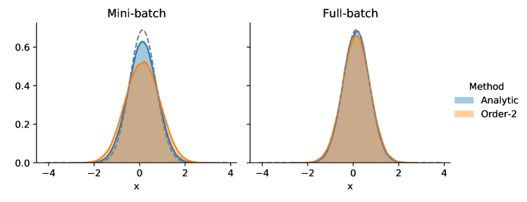
Figure 6: Histograms of stationary distributions (100K samples). The grey dotted line denotes the true posterior density. Irrespectively of order, mini-batching prevents from convergence to true posterior.

We further support our numerical evidence with a through theoretical exploration in Section E.2.

E.2 Derivation of the analytical integrators

We consider the dynamics of Eq. 3, where for simplicity $\mathbf{M}=1$. We then have, remembering $\mathbf{z}(t)=\begin{bmatrix}r(t)\\ \theta(t)\end{bmatrix}$, the following sde

$$d\mathbf{z}(t)=\begin{bmatrix}-C&-1\\ 1&0\end{bmatrix}\begin{bmatrix}r(t)\\ {\sigma_{l}^{-2}}(\theta(t)-\frac{x_{1}+x_{2}}{v})\end{bmatrix}dt+\begin{bmatrix}\sqrt{2C}dw(t)\\ 0\end{bmatrix},$$ (85)

that we rewrite in the more convenient form

$$d\mathbf{z}(t)=\begin{bmatrix}-C&-{\sigma_{l}^{-2}}\\ 1&0\end{bmatrix}\left(\mathbf{z}(t)-\begin{bmatrix}0\\ \bar{x}\end{bmatrix}\right)dt+\begin{bmatrix}\sqrt{2C}dw(t)\\ 0\end{bmatrix},$$ (86)

where $\bar{x}=\frac{x_{1}+x_{2}}{v}$.

Starting from initial conditions $\mathbf{z}(0)=\mathbf{z}_{0}$, we can shown that the system has analytic solution

$$\mathbf{z}(t)=\exp\left(t\mathbf{A}\right)\left(\mathbf{z}_{0}-\begin{bmatrix}0\\ \bar{x}\end{bmatrix}\right)+\begin{bmatrix}0\\ \bar{x}\end{bmatrix}+\int\limits_{s=0}^{t}\exp\left((t-s)\mathbf{A}\right)\begin{bmatrix}\sqrt{2C}dw(s)\\ 0\end{bmatrix}$$ (87)

where for simplicity we have defined $\mathbf{A}=\begin{bmatrix}-C&-{\sigma_{l}^{-2}}\\ 1&0\end{bmatrix}$. Considering that ${\sigma_{l}^{-2}},C>0$ simple calculations show that the eigenvalues of $\mathbf{A}$ have negative real part, ensuring that as $t\rightarrow\infty$ we have $\exp\left(t\mathbf{A}\right)\rightarrow\mathbf{0}$.

A probabilistically equivalent representation of eq. Eq. 87 is the following

$$\mathbf{z}(t)=\exp\left(t\mathbf{A}\right)\left(\mathbf{z}_{0}-\begin{bmatrix}0\\ \bar{x}\end{bmatrix}\right)+\begin{bmatrix}0\\ \bar{x}\end{bmatrix}+\mathbf{n},$$ (88)

where

$$\mathbf{n}\sim\mathcal{N}\left(\mathbf{0},\int\limits_{s=0}^{t}\exp\left((t-s)\mathbf{A}\right)\begin{bmatrix}2C&0\\ 0&0\end{bmatrix}\exp\left((t-s)\mathbf{A}^{\top}\right)ds\right).$$ (89)

Equation Eq. 88 guarantees that it is possible to build a numerical integrator for any chosen step size $\eta$ that simulates exactly the dynamics, corresponding to an arbitrarily high order of weak integration.

Convergence to the posterior

We then explore the transition probability starting from a given initial state $\mathbf{z}_{0}$ induced by such a numerical integrator with step size $\eta$

$$p(\mathbf{z}(\eta)|\mathbf{z}(0)=\mathbf{z}_{0})=$$

$$\mathcal{N}\left(\mathbf{z}(\eta);\exp\left(\eta\mathbf{A}\right)\left(\mathbf{z}_{0}-\begin{bmatrix}0\\ \bar{x}\end{bmatrix}\right)+\begin{bmatrix}0\\ \bar{x}\end{bmatrix},\int\limits_{s=0}^{\eta}\exp\left((\eta-s)\mathbf{A}\right)\begin{bmatrix}2C&0\\ 0&0\end{bmatrix}\exp\left((\eta-s)\mathbf{A}^{\top}\right)ds\right).$$ (90)

As shown in Section E.2.1, the covariance matrix of the distribution Section E.2 can be expressed as

$$\int\limits_{s=0}^{\eta}\exp\left((\eta-s)\mathbf{A}\right)\begin{bmatrix}2C&0\\ 0&0\end{bmatrix}\exp\left((\eta-s)\mathbf{A}^{\top}\right)ds=\begin{bmatrix}1&0\\ 0&{\sigma_{l}^{2}}\end{bmatrix}-\exp\left(\eta\mathbf{A}\right)\begin{bmatrix}1&0\\ 0&{\sigma_{l}^{2}}\end{bmatrix}\exp\left(\eta\mathbf{A}^{\top}\right),$$ (91)

and consequently, we can rewrite Section E.2 as

$$p(\mathbf{z}(\eta)|\mathbf{z}(0)=\mathbf{z}_{0})=$$

$$\mathcal{N}\left(\mathbf{z}(\eta);\exp\left(\eta\mathbf{A}\right)\left(\mathbf{z}_{0}-\begin{bmatrix}0\\ \bar{x}\end{bmatrix}\right)+\begin{bmatrix}0\\ \bar{x}\end{bmatrix},\mathbf{\Sigma}(\eta)\right),$$ (92)

where we introduced the $\mathbf{\Sigma}(\eta)=\begin{bmatrix}1&0\\ 0&{\sigma_{l}^{2}}\end{bmatrix}-\exp\left(\eta\mathbf{A}\right)\begin{bmatrix}1&0\\ 0&{\sigma_{l}^{2}}\end{bmatrix}\exp\left(\eta\mathbf{A}^{\top}\right)$.

Importantly, we have that $\rho_{ss}(\mathbf{z})$ is the stationary distribution of the stochastic process, if and only if the following holds:

$$\rho_{ss}(\mathbf{z}^{*})=\int p(\mathbf{z}(\eta)=\mathbf{z}^{*}|\mathbf{z}(0)=\mathbf{z})\rho_{ss}(\mathbf{z})d\mathbf{z}$$ (93)

where obviously the equality must hold for all $\eta$. To check that eq. Eq. 93 holds with:

$$\rho_{ss}(\mathbf{z})=\mathcal{N}(r;0,1)\,\mathcal{N}\left(\theta;\frac{x_{1}+x_{2}}{v},\sigma_{l}^{2}\right)=\mathcal{N}\left(\mathbf{z};\begin{bmatrix}0\\ \bar{x}\end{bmatrix},\begin{bmatrix}1&0\\ 0&\sigma_{l}^{2}\end{bmatrix}\right)$$ (94)

we substitute directly:

$$\int p(\mathbf{z}(\eta)=\mathbf{z}^{*}|\mathbf{z}(0)=\mathbf{z})\rho_{ss}(\mathbf{z})d\mathbf{z}=$$

$$\int\mathcal{N}\left(\mathbf{z}^{*};\exp\left(\eta\mathbf{A}\right)\left(\mathbf{z}-\begin{bmatrix}0\\ \bar{x}\end{bmatrix}\right)+\begin{bmatrix}0\\ \bar{x}\end{bmatrix},\mathbf{\Sigma}(\eta)\right)\mathcal{N}\left(\mathbf{z};\begin{bmatrix}0\\ \bar{x}\end{bmatrix},\begin{bmatrix}1&0\\ 0&\sigma_{l}^{2}\end{bmatrix}\right)d\mathbf{z}$$

$$=\mathcal{N}\left(\mathbf{z}^{*};\exp\left(\eta\mathbf{A}\right)\left(\begin{bmatrix}0\\ \bar{x}\end{bmatrix}-\begin{bmatrix}0\\ \bar{x}\end{bmatrix}\right)+\begin{bmatrix}0\\ \bar{x}\end{bmatrix},\mathbf{\Sigma}(\eta)+\exp\left(\eta\mathbf{A}\right)\begin{bmatrix}1&0\\ 0&{\sigma_{l}^{2}}\end{bmatrix}\exp\left(\eta\mathbf{A}^{\top}\right)\right)$$

$$=\mathcal{N}\left(\mathbf{z}^{*};\begin{bmatrix}0\\ \bar{x}\end{bmatrix},\begin{bmatrix}1&0\\ 0&{\sigma_{l}^{2}}\end{bmatrix}\right)$$

proving that the stationary distribution is indeed the desired one.

Failure of convergence in the case of mini-batches

In the following, we show that when considering mini-batches instead, we fail to converge to the true posterior. Importantly this is true even with the analytical solution for the steps of the integrator, stressing that numerical integration and mini-batching have two independent effects. With mini-batches, at every step of the integration a $x_{1},x_{2}$ are sampled with probability $\frac{1}{2}$.

Instead of simulating eq. Eq. 86 at every step of the numerical integration, the following stochastic process is then considered:

$$d\mathbf{z}(t)=\begin{bmatrix}-C&-{\sigma_{l}^{-2}}\\ 1&0\end{bmatrix}\left(\mathbf{z}(t)-\begin{bmatrix}0\\ \bar{x}_{i}\end{bmatrix}\right)dt+\begin{bmatrix}\sqrt{2C}dw(t)\\ 0\end{bmatrix}$$ (95)

where, $\bar{x}_{i}=\frac{2x_{i}}{v}$, and $i=1$ or $i=2$ is sampled randomly.

Similarly to the previous case it is possible to construct a numerical integrator that solves exactly the dynamics, this time with the potential computed using randomly only one of the two datapoints. The transition probability induced by such an integrator will then be equal to:

$$p(\mathbf{z}(\eta)=\mathbf{z}^{*}|\mathbf{z}(0)=\mathbf{z}_{0}) =\frac{1}{2}\mathcal{N}\left(\mathbf{z}^{*};\exp\left(\eta\mathbf{A}\right)\left(\mathbf{z}_{0}-\begin{bmatrix}0\\ \bar{x}_{1}\end{bmatrix}\right)+\begin{bmatrix}0\\ \bar{x}_{1}\end{bmatrix},\mathbf{\Sigma}(\eta)\right)$$

$$+\frac{1}{2}\mathcal{N}\left(\mathbf{z}^{*};\exp\left(\eta\mathbf{A}\right)\left(\mathbf{z}_{0}-\begin{bmatrix}0\\ \bar{x}_{2}\end{bmatrix}\right)+\begin{bmatrix}0\\ \bar{x}_{2}\end{bmatrix},\mathbf{\Sigma}(\eta)\right)$$ (96)

$$=\frac{1}{2}f_{1}(\mathbf{z}^{*},\eta,\mathbf{z}_{0})+\frac{1}{2}f_{2}(\mathbf{z}^{*},\eta,\mathbf{z}_{0}),$$ (97)

where $f_{1},f_{2}$ are the two Gaussian transition probabilities. Importantly, this allows to state the following central statement: the distribution $p(\theta|\mathcal{D})$ is not the stationary distribution of the process. This claim can be proven by contradiction. Suppose that the stationary distribution is the one of interest, $\mathcal{N}\left(\mathbf{z};\begin{bmatrix}0\\ \bar{x}\end{bmatrix},\begin{bmatrix}1&0\\ 0&{\sigma_{l}^{2}}\end{bmatrix}\right)$. Performing one step of integration the new distribution will be of the form:

$$\rho_{new}(\mathbf{z}^{*}) =\int\left(\frac{1}{2}f_{1}(\mathbf{z}^{*},\eta,\mathbf{z})+\frac{1}{2}f_{2}(\mathbf{z}^{*},\eta,\mathbf{z})\right)\rho_{ss}(\mathbf{z})d\mathbf{z}$$ (98)

$$=\frac{1}{2}\mathcal{N}\left(\mathbf{z}^{*};\exp\left(\eta\mathbf{A}\right)\left(\begin{bmatrix}0\\ \bar{x}\end{bmatrix}-\begin{bmatrix}0\\ \bar{x}_{1}\end{bmatrix}\right)+\begin{bmatrix}0\\ \bar{x}\end{bmatrix},\begin{bmatrix}1&0\\ 0&{\sigma_{l}^{2}}\end{bmatrix}\right)$$

$$+\frac{1}{2}\mathcal{N}\left(\mathbf{z}^{*};\exp\left(\eta\mathbf{A}\right)\left(\begin{bmatrix}0\\ \bar{x}\end{bmatrix}-\begin{bmatrix}0\\ \bar{x}_{2}\end{bmatrix}\right)+\begin{bmatrix}0\\ \bar{x}\end{bmatrix},\begin{bmatrix}1&0\\ 0&{\sigma_{l}^{2}}\end{bmatrix}\right)$$ (99)

$$\neq\rho_{ss}(\mathbf{z}^{*}).$$ (100)

By definition, we should have the functional equivalence between $\rho_{new}$ and $\rho_{ss}$. Equation Eq. 98 implies however that after the mixture transition probability the new density $\rho_{new}$ will be a mixture of Gaussian distributions, and consequently $\rho_{new}\neq\rho_{ss}$. This concludes the demonstration that the stationary distribution is not the one of interest.

E.2.1 Derivation of eq. Eq. 91

Define:

$$\mathbf{K}(t)=\int\limits_{s=0}^{t}\exp\left((t-s)\mathbf{A}\right)\begin{bmatrix}2C&0\\ 0&0\end{bmatrix}\exp\left((t-s)\mathbf{A}^{\top}\right)ds,$$ (101)

and

$$\mathbf{S}(t)=\begin{bmatrix}1&0\\ 0&{\sigma_{l}^{2}}\end{bmatrix}-\exp\left(t\mathbf{A}\right)\begin{bmatrix}1&0\\ 0&{\sigma_{l}^{2}}\end{bmatrix}\exp\left(t\mathbf{A}^{\top}\right).$$ (102)

Immediately we see that $\mathbf{K}(0)=\mathbf{S}(0)=\mathbf{0}$.

The derivative of $\mathbf{K}(t)$ has expression:

$$\frac{d\mathbf{K}(t)}{dt} =\exp\left((t-t)\mathbf{A}\right)\begin{bmatrix}2C&0\\ 0&0\end{bmatrix}\exp\left((t-t)\mathbf{A}^{\top}\right)$$

$$+\mathbf{A}\int\limits_{s=0}^{t}\exp\left((t-s)\mathbf{A}\right)\begin{bmatrix}2C&0\\ 0&0\end{bmatrix}\exp\left((t-s)\mathbf{A}^{\top}\right)ds$$

$$+\int\limits_{s=0}^{t}\exp\left((t-s)\mathbf{A}\right)\begin{bmatrix}2C&0\\ 0&0\end{bmatrix}\exp\left((t-s)\mathbf{A}^{\top}\right)ds\mathbf{A}^{\top}$$

$$=\begin{bmatrix}2C&0\\ 0&0\end{bmatrix}+\mathbf{A}\mathbf{K}(t)+\mathbf{K}(t)\mathbf{A}^{\top}.$$

Similarly we have:

$$\frac{d\mathbf{S}(t)}{dt} =-\mathbf{A}\exp\left(t\mathbf{A}\right)\begin{bmatrix}1&0\\ 0&{\sigma_{l}^{2}}\end{bmatrix}\exp\left(t\mathbf{A}^{\top}\right)-\exp\left(t\mathbf{A}\right)\begin{bmatrix}1&0\\ 0&{\sigma_{l}^{2}}\end{bmatrix}\exp\left(t\mathbf{A}^{\top}\right)\mathbf{A}^{\top}$$

$$=-\mathbf{A}\left(\begin{bmatrix}1&0\\ 0&{\sigma_{l}^{2}}\end{bmatrix}-\mathbf{S}(t)\right)-\left(\begin{bmatrix}1&0\\ 0&{\sigma_{l}^{2}}\end{bmatrix}-\mathbf{S}(t)\right)\mathbf{A}^{\top}.$$

Since $\mathbf{A}\begin{bmatrix}1&0\\ 0&{\sigma_{l}^{2}}\end{bmatrix}=\begin{bmatrix}-C&-1\\ 1&0\end{bmatrix}$, we can prove

$$\frac{d\mathbf{S}(t)}{dt}=\begin{bmatrix}2C&0\\ 0&0\end{bmatrix}+\mathbf{A}\mathbf{S}(t)+\mathbf{S}(t)\mathbf{A}^{\top}.$$

Definining the difference matrix $\mathbf{H}(t)=\mathbf{K}(t)-\mathbf{S}(t)$ we recognize that it satisfies the differential equation

$$\frac{d\mathbf{H}(t)}{dt}=\mathbf{A}\mathbf{H}(t)+\mathbf{H}(t)\mathbf{A}^{\top}$$

that has explicit solution

$$\mathbf{H}(t)=\exp\left(t\mathbf{A}\right)\mathbf{H}(0)\exp\left(t\mathbf{A}^{\top}\right)$$ (103)

Since $\mathbf{H}(0)=\mathbf{0}$ we conclude $\mathbf{H}(t)=\mathbf{0}$ proving the desired equality.

Appendix F EXPERIMENTS: ADDITIONAL DETAILS

F.1 Experimental setup

Throughout our experimental campaign, we work on a number of datasets from the UCI repository. For each dataset, we have considered $5$ random splits into training and test sets; for the regression datasets, we have adopted the splits in Mukhoti et al. (2018) which are available online under the Creative Commons licence. The primary point of interest is in this work is the predictive distribution over the test set and how this deviates from the true posterior. Table 1 and Table 2 summarize the details of the regression and classification datasets in this work. In the same tables we report some error metrics; the latter are not a central part of the evaluation of this paper, but they are simply indicative of the performance of shmc. Our implementation is loosely based on the PYSGMCMC framework.

Network architecture.

Throughout this experimental campaign, we consider bnns featuring $L$ layers, where each layer is defined as follows:

$$f_{l}(\mathbf{x})=\frac{1}{\sqrt{D_{l-1}}}\mathbf{W}_{l}\,\varphi(f_{l-1}(\mathbf{x}))+\mathbf{b}_{l},\quad l\in\{1,...,L+1\},$$ (104)

where $\varphi$ is a non-linear activation function. The model parameters are summarized as $\boldsymbol{\theta}\equiv\{\mathbf{W}_{l}\in\mathbb{R}^{D_{l}\times D_{l-1}},\mathbf{W}_{l}\in\mathbb{R}^{D_{l}\times D_{l-1}}\}$, and they denote the matrix of weights and the vector of biases for layer $l$. Note that we divide by the square root of the input dimension $D_{l-1}$; this scheme is known as the NTK parameterization (Jacot et al., 2018; Lee et al., 2020), and it ensures that the asymptotic variance neither explodes nor vanishes. In this context, we place a standard Gaussian prior for both weights and biases, i.e. $p(\boldsymbol{\theta})=\mathcal{N}(0,I)$.

Regression and classification tasks.

For regression tasks we consider bnns with 4 layers and 50 nodes per layer with ReLU activation. Table 1 outlines the predictive performance of shmc for four regression datasets (boston, concrete, energy and yacht), as well as the noise variance $\sigma^{2}$ used in each case. We have drawn $200$ samples from the posterior and the regression performance is evaluated in terms of root mean squared error (rmse) and mean negative log-likelihood mnll. In order to put these values into perspective, we also show the results for the adaptive sghmc scheme from Springenberg et al. (2016) featuring a network of identical structure as in our setup. In both cases, the full-batch gradient was used.

Table 1: Regression results for bnns with 4 layers and 50 nodes per layer with ReLU activation. For sghmc we follow Springenberg et al. (2016).

	Training Size	Test Size		Test rmse$(\downarrow)$		Test mnll$(\downarrow)$
DATASET			$\sigma^{2}$	shmc	sghmc	shmc	sghmc
Boston	455	51	0.2	2.821$\pm$0.61	2.825$\pm$0.63	2.600$\pm$0.09	2.600$\pm$0.09
Concrete	927	103	0.05	4.907$\pm$0.39	4.833$\pm$0.46	2.971$\pm$0.07	2.948$\pm$0.09
Energy	691	77	0.01	0.501$\pm$0.07	0.489$\pm$0.07	1.191$\pm$0.07	1.120$\pm$0.03
Yacht	277	31	0.005	0.420$\pm$0.12	0.436$\pm$0.13	1.180$\pm$0.02	1.176$\pm$0.02

For classification we consider ionosphere and vehicle from UCI, for which we sample from ReLU bnns with 2 layers and 50 nodes per layer. We have drawn $200$ samples from the posterior, and the predictive accuracy and test mnll of shmc can be seen in Table 2, where we also show the performance of the adaptive version of sghmc (Springenberg et al., 2016). The results have been very similar for these two cases; this has been expected, as both methods are supposed to converge to the same posterior.

Table 2: Classification results for bnns with 2 layers and 50 nodes per layer with ReLU activation. For sghmc we follow Springenberg et al. (2016).

		Training Size	Test Size	Test accuracy$(\uparrow)$		Test mnll$(\downarrow)$
DATASET	Classes			shmc	sghmc	shmc	sghmc
Ionosphere	2	301	34	0.920$\pm$0.03	0.916$\pm$0.02	0.294$\pm$0.04	0.295$\pm$0.04
Vehicle	4	646	200	0.777$\pm$0.02	0.783$\pm$0.02	0.588$\pm$0.03	0.588$\pm$0.03

Synthetic regression example.

We also consider as simple regression model applied on the synthetic one-dimensional dataset of Fig. 7. In this case we choose a linear model with fixed basis functions, in order to demonstrate shmc convergence in a fully controlled environment where the true posterior can be calculated analytically. We consider $D=256$ trigonometric basis functions: $f(x)=\sqrt{\nicefrac{{2}}{{D}}}\,\mathbf{w}^{\top}\cos(\omega x-\pi/4)$, where $\mathbf{w}\in\mathbb{R}^{D\times 1}$ contains the weights of $D$ features and $\omega\in\mathbb{R}^{D\times 1}$ is a vector of fixed frequencies. In the experiments that follow, we have a Gaussian likelihood with variance $0.1$ and prior $p(\mathbf{w})=\mathcal{N}(0,I_{D})$. The predictive posterior can be seen in Fig. 7, where the test set consists of $200$ uniformly distributed points.

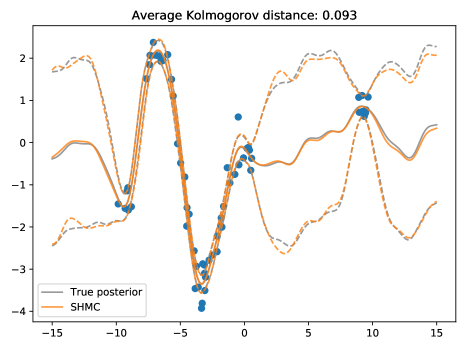
Figure 7: True and shmc predictive posterior on a synthetic dataset.

F.2 Comparison framework and convergence to posterior

Comparing predictive distributions.

In this work, we explore the behavior of a number of methods by comparing the predictive distribution given by a particular setting to the distribution of an oracle. The comparison is performed in terms of one-dimensional predictive marginals using $200$ samples: for each test point we evaluate the Kolmogorov distance between the predictive distribution and the oracle. We then report the average distance over the test set. The Kolmogorov distance takes values between 0 and 1. In Fig. 7 we show an one-dimensional regression example where the average distance values over the test set is smaller than $0.1$.

Self-distance.

When we compare the distance between empirical distribution, this will never be exactly zero. In order to determine whether a given sample is a sufficiently good approximation for a target distribution, we have to compare the corresponding distance value to the self-distance. The latter can be evaluated by resampling from the oracle posterior distribution: for each oracle we consider $5$ independent runs producing $200$ samples each, which are used to estimate the Kolmogorov self-distance. In the results of Fig. 8, Fig. 9 and Fig. 10, the shaded area denotes the 0.05 and 0.95-quantiles of the self-distance distribution.

Methods summary.

The main focus of this experimental campaign is to explore how shmc is affected by changes of step size and batch size, and to observe whether the introduction of mini-batches induces a convergence bottleneck in practice or not. For shmc, we consider $4$ integrators: leapfrog which is provably of order 1, symmetric (Chen et al., 2015) and lie-trotter (Section 4) which are of order 2, and mt3 (Milstein and Tretyakov, 2003) which is a third order integrator. We also compare against sghmc (Chen et al., 2014).

Computational summary.

At this point, we note that each block in Fig. 8, Fig. 9 and Fig. 10 corresponds to $5$ random splits or seeds. For most datasets, drawing 200 samples for the smallest step size (i.e. $0.001$) required 15–20 minutes. Such a small step size has been necessary in order to demonstrate convergence for small batch sizes. A full exploration of the methods and integrators for a single split (or seed) of a single dataset required approximately one day of computation on a computer cluster featuring Intel® Xeon® CPU @2.00GHz. It has not been possible to do this kind of exploration in a meaningful way for larger datasets, yet we believe that the existing results are sufficient to demonstrate our theoretical claims.

Convergence.

In order to reason about convergence in the experiments that follow, we have taken great care to approximate the true posterior with sghmc, which we treat as oracle. For the oracles we consider full-batch and $\eta=0.005$ in all cases, except for the linear model where the true posterior has been analytically tractable. The simulation time has been determined by adjusting the thinning parameter so that lag-1 autocorrelation (acf(1)) was considered as acceptable. In practice we keep one sample every $500$ steps (i.e. thinning), and we discard the first $2000$ steps. Then for each oracle, the simulation time was doubled one more time, but that resulted in no significant difference in the predictive distribution. The summary of acf(1) values that correspond to the oracles used in this work can be found in Table 3. As a final remark, we note that for each combination of dataset and model, all random walks cover the same simulation time. The CPU time is thus determined by the step size $\eta$: a larger value for $\eta$ implies that a smaller number of steps is required to simulate a certain system, as the thinning parameter is adjusted accordingly.

Table 3: Lag 1 autocorrelation for the sghmc algorithms used as oracles.

DATASET	acf(1)
Boston	0.09
Concrete	0.23
Energy	0.05
Yacht	0.05
Ionosphere	0.17
Vehicle	0.18

F.3 Extended regression and classification results

In this section we present the results of step size and batch size exploration for the entirety of datasets considered. In all cases, we set $C=5$; we find this to be a reasonable choice, as we see in the exploration of Section F.4.

Figure 8 focuses on the comparison between shmc with different integrators (leapfrog, symmetric, lie-trotter and mt3) and sghmc. This is an extended version of Fig. 4 of the main paper; we include all the datasets considered, as well as a more fine grained exploration of the batch size.

Figure 9 is an extended version of Fig. 5 of the main paper. It contains a complete account of the exploration of the integration length $N_{l}$ for the (generalized) lie-trotter integrator.

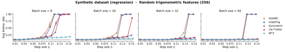
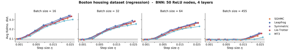
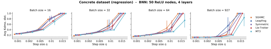
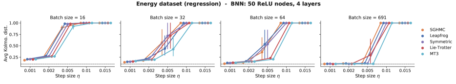
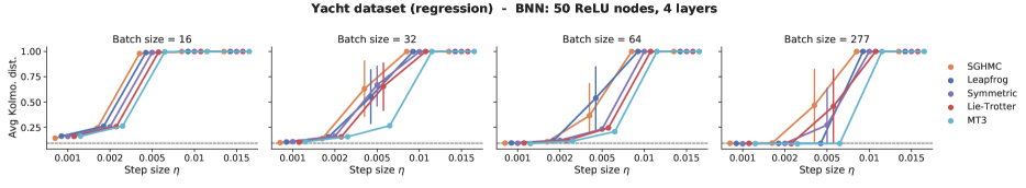
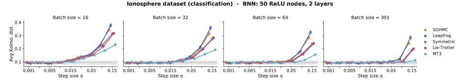
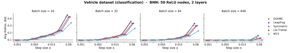
Figure 8: Exploration of step size and batch size for different Hamiltonian-based methods; the grey dotted line denotes the self-distance for the distribution of the oracle.

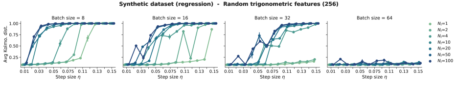
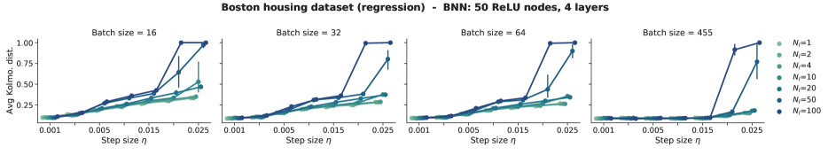
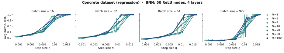
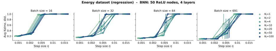
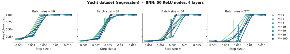
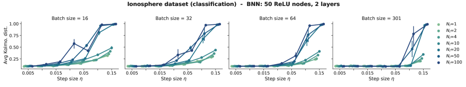
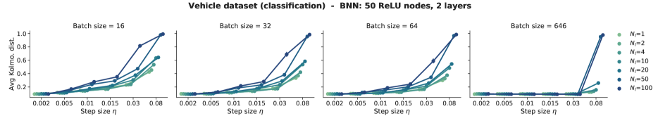
Figure 9: Generalized lie-trotter: Exploration of step size and batch size for different values of the (deterministic) integration length $N_{l}$. The grey dotted line denotes the self-distance for the distribution of the oracle.

F.4 Exploration of the friction constant $C$

The user-specified constant $C$ appears twice in Eq. 3: in the friction term and in the stochastic diffusion term of the sde. Although Theorem 1 implies that any choice for $C>0$ will maintain the desired stationary distribution (i.e. $\rho_{ss}(\boldsymbol{\theta})\propto\exp(-U(\boldsymbol{\theta}))$), the transient dynamics of the sde do change as we have seen in the sample paths of Fig. 2. It is generally expected that as $C$ approaches $0$, the sample paths approach the deterministic behavior of an ode. On the other hand, if $C$ is too large, the stochastic process degenerates to the standard Brownian motion. It is expected that either of these extremes would hurt the usability of sde simulation as a sampling scheme, but the exact effect of $C$ is not apparent.

In this section, we experimentally examine how a certain choice for $C$ affects practical convergence to the desired posterior in conjunction with the step size $\eta$ as well as the mini-batch size. Figure 10 summarizes an extensive exploration of $C$ for all the models and datasets considered in this work using the leapfrog integrator, with $C$ varying from $0.5$ to $100$. Again, we measure the average Kolmogorov distance from the true predictive posterior for the test points, and we want to see whether the curve for varying $\eta$ and batch size approaches the band of self-distance.

As a general remark, the desired convergence properties are not too sensitive to the constant $C$. Although, the optimal value for $C$ does depend on the dynamics induced by a particular dataset and model, it appears that there is a wide range of values that can be considered as acceptable. For most of the cases considered, a value between $5$ and $10$ seems to produce reasonable results. Nevertheless, we think that some manual exploration would still be required for a new dataset.

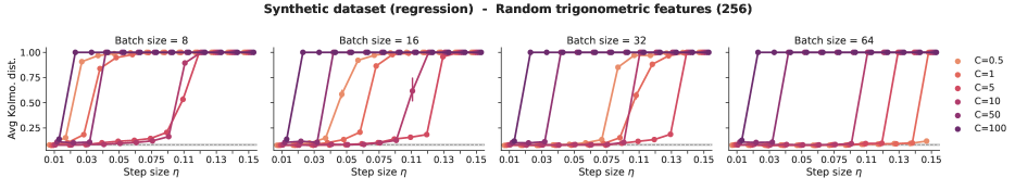
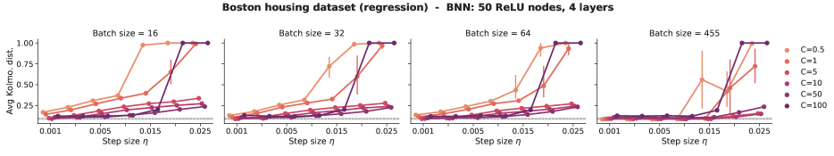
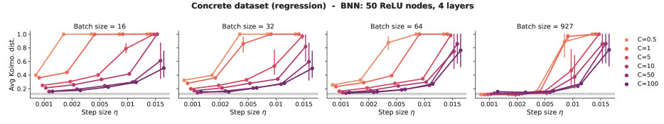
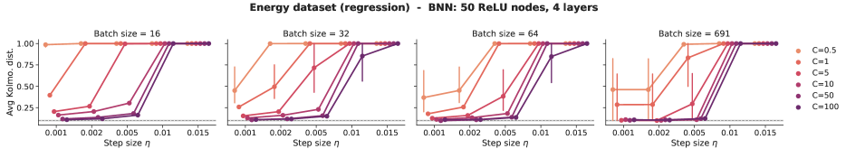
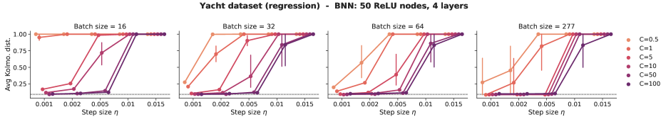
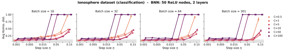
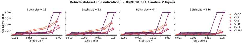
Figure 10: Exploration of step size and batch size for different values of a scalar friction coefficient $C$. The grey dotted line denotes the self-distance for the distribution of the oracle. leapfrog is used in all cases.

References

• Abdulle et al. (2014) A. Abdulle, G. Vilmart, and K. C. Zygalakis. High order numerical approximation of the invariant measure of ergodic sdes. SIAM Journal on Numerical Analysis, 52(4):1600–1622, 2014.
• Abdulle et al. (2015) A. Abdulle, G. Vilmart, and K. C. Zygalakis. Long time accuracy of Lie-Trotter splitting methods for Langevin dynamics. SIAM Journal on Numerical Analysis, 53(1):1–16, 2015.
• Ahn et al. (2012) S. Ahn, A. Korattikara, and M. Welling. Bayesian posterior sampling via stochastic gradient Fisher scoring. In International Conference on Machine Learning, pages 1771–1778, 2012.
• Betancourt (2015) M. Betancourt. The fundamental incompatibility of scalable Hamiltonian Monte Carlo and naive data subsampling. In F. Bach and D. Blei, editors, International Conference on Machine Learning, volume 37 of Proceedings of Machine Learning Research, pages 533–540, Lille, France, 07–09 Jul 2015.
• Betancourt et al. (2018) M. Betancourt, M. I. Jordan, and A. C. Wilson. On symplectic optimization. arXiv preprint arXiv:1802.03653, 2018.
• Bishop (2006) C. M. Bishop. Pattern recognition and machine learning. Springer, 1st ed. 2006. corr. 2nd printing 2011 edition, 2006. ISBN 0387310738.
• Bou-Rabee and Owhadi (2010) N. Bou-Rabee and H. Owhadi. Long-run accuracy of variational integrators in the stochastic context. SIAM Journal on Numerical Analysis, 48(1):278–297, 2010.
• Chaudhari and Soatto (2018) P. Chaudhari and S. Soatto. Stochastic gradient descent performs variational inference, converges to limit cycles for deep networks. In 2018 Information Theory and Applications Workshop (ITA), pages 1–10. IEEE, 2018.
• Chen et al. (2015) C. Chen, N. Ding, and L. Carin. On the convergence of stochastic gradient MCMC algorithms with high-order integrators. Advances in neural information processing systems, 28:2278–2286, 2015.
• Chen et al. (2014) T. Chen, E. Fox, and C. Guestrin. Stochastic gradient Hamiltonian Monte Carlo. In International conference on machine learning, pages 1683–1691, 2014.
• Childs and Su (2019) A. M. Childs and Y. Su. Nearly optimal lattice simulation by product formulas. Physical review letters, 123(5):050503, 2019.
• Childs et al. (2019) A. M. Childs, A. Ostrander, and Y. Su. Faster quantum simulation by randomization. Quantum, 3:182, 2019.
• Childs et al. (2021) A. M. Childs, Y. Su, M. C. Tran, N. Wiebe, and S. Zhu. Theory of Trotter error with commutator scaling. Physical Review X, 11(1):011020, 2021.