Adversarial examples within the training distribution:
A widespread challenge

Abstract

Despite a plethora of proposed theories, understanding why deep neural networks are susceptible to adversarial attacks remains an open question. A promising recent strand of research investigates adversarial attacks within the training data distribution, providing a more stringent and worrisome definition for these attacks. These theories posit that the key issue is that in high dimensional datasets, most data points are close to the ground-truth class boundaries. This has been shown in theory for some simple data distributions, but it is unclear if this theory is relevant in practice. Here, we demonstrate the existence of in-distribution adversarial examples for object recognition. This result provides evidence supporting theories attributing adversarial examples to the proximity of data to ground-truth class boundaries, and calls into question other theories which do not account for this more stringent definition of adversarial attacks. These experiments are enabled by our novel gradient-free, evolutionary strategies (ES) based approach for finding in-distribution adversarial examples in 3D rendered objects, which we call CMA-Search.

1 Introduction

Figure 1: In-distribution adversarial examples. This schematic highlights the difference between typical (out-of-distribution) and in-distribution adversarial examples. We train object recognition models on a large scale training data of $0.5$ million images sampled from known, parametric distribution of camera and light variations (depicted using  ). Despite great success in correctly classifying newly sampled test points from the training data distribution (X), our CMA-Search method shows that it is possible to find plenty of adversarial examples which lie within the training distribution (X^′′). Unlike existing methods that add noise to the image resulting in out-of-distribution adversarial examples (X^′′), CMA-Search searches within the training distribution to find adversarial examples. We find a widespread presence of in-distribution adversarial examples for object recognition.

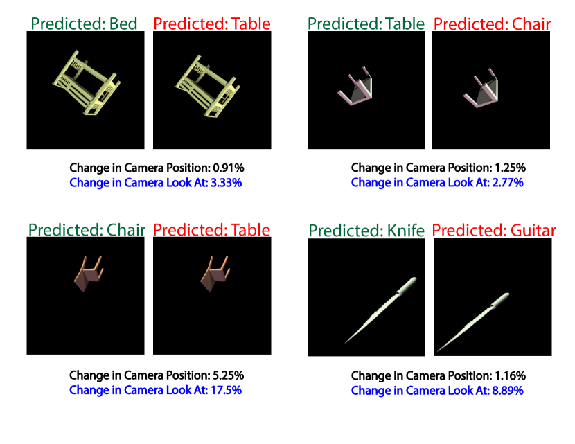
Figure 2: Sample in-distribution adversarial examples identified using CMA-Search with camera parameters. Starting with the correctly predicted images, our evolutionary-strategy based method (CMA-Search) explores the vicinity of camera parameters for subtle 3D perspective changes that lead to misclassification. These in-distribution adversarial examples are often found very close to the correctly classified starting image. In the figure we report the percentage of change in Camera Position and Camera Look At parameters necessary to induce the misclassification.

Understanding the mechanisms enabling adversarial attacks on deep neural networks remains an open and elusive problem in machine learning. Despite a plethora of works attempting to explain these attacks, posited theories are largely disconnected and focus on specific considerations such as attributing adversarial attacks to the tilting tanay2016boundary or the curvature  fawzi2016robustness of the learned decision boundary, the dimension of the data manifold shamir2019simple ; shamir2021dimpled , data distribution shifts ford2019adversarial , the presence of non-robust features ilyas2019adversarial ; tsipras2018robustness , lack of data schmidt2018adversarially , and computational complexity bubeck2019adversarial ; nakkiran2019adversarial , among others. It remains unclear which of these theories are more valid in practice and can fully explain adversarial attacks on object recognition models.

Adversarial examples are usually defined as perturbed inputs which cause classification networks to make an error. However, there is no constraint enforced on the resulting adversarial example’s position with respect to the training data distribution. Recently, a strand of theoretical works have provided compelling evidence for adversarial examples that lie within the training distribution (gilmer2018relationship, ; fawzi2018adversarial, ; shafahi2018adversarial, ; mahloujifar2019curse, ; diochnos2018adversarial, ; dohmatob2018limitations, ). Such in-distribution examples provide a more stringent definition of adversarial examples than typically used in the theories mentioned above by enforcing that the resulting examples lie within the training data distribution. This newly discovered phenomenon of in-distribution adversarial examples presents an opportunity to compare different theories, and to validate which ones can explain these findings. Furthermore, such examples are highly concerning as unlike typical adversarial examples these do not require adding synthetically engineered perturbations by an external malicious agent since these examples are already within the training data distribution.

The key insight at the heart of these theoretical works is that most data points are close to the ground-truth class boundaries, for high-dimensional data distributions. Thus, slight deviations between the learned and the ground-truth class boundaries causes in-distribution adversarial examples given the proximity of these points to these boundaries. For brevity, we refer to this theory as the ground-truth boundary theory.

While this theory demonstrates that the phenomenon of adversarial examples runs far deeper than the added perturbations resulting in samples from outside the data distribution, works investigating the ground-truth boundary theory make strong simplifying assumptions about the data distributions which may not hold true in practice. This includes assuming that the data is generated from a smooth generative model fawzi2018adversarial , belongs to a Levy family mahloujifar2019curse , satisfies the $W_{2}$ Talagrand transportation-cost inequality, lies on a uniform hypercube shafahi2018adversarial ; diochnos2018adversarial , or on disjoint concentric shells gilmer2018relationship . As noted in these papers, it is unclear whether these theoretical findings are relevant in practice, as these assumptions may not be true for images of real-world objects.

Here, we seek to reconcile this disconnect by asking whether this theory extends to image data for object recognition. A positive answer would provide compelling evidence in support of the ground-truth boundary theory being the primary mechanism driving adversarial examples.

To find in-distribution adversarial attacks, we introduce an evolution-strategy based search method that we call CMA-Search. Most existing adversarial attack methods rely on derivative-based search which suffer from two problems. Firstly, they cannot efficiently find in-distribution adversarial examples at low dimensions gilmer2018relationship . Secondly, it is unclear if the adversarial sample found after noise addition still belongs to the training distribution. In contrast, starting with a correctly classified input CMA-Search searches the vicinity of input parameters to find in-distribution adversarial examples. To reflect this, we chose to name our approach an adversarial-search method, as opposed to an adversarial attack method. Inspired by recent works using computer graphics to create controlled datasets for investigating neural networks madan2020capability ; varol17_surreal ; mu2020learning ; zeng2019adversarial , we introduce a procedural computer graphics pipeline. Our pipeline allows us to generate a large-scale dataset with complete control over camera and lighting variations. This offers us explicit, parametric control over the training distribution similar to theoretical works, enabling us to investigate in-distribution adversarial examples with complex images of objects.

These experiments lead us to our key finding—there is a widespread presence of adversarial images within the training distribution, as summarized in Fig. 1. To foreshadow our results, CMA-Search can find such an adversarial example for over $71\%$ cases with an average change of only $1.83\%$ in the camera position, in $42\%$ cases with an average change of only $6.52\%$ in the lighting conditions. These examples are depicted in Fig. 2. Finally, we also extend our method in conjunction with a novel view synthesis pipeline (tucker2020single, ) to find adversarial examples in the vicinity of ImageNet (deng2009imagenet, ) images for a ResNet model and the recently released OpenAI CLIP model (radford2021learning, ). These results on in-distribution adversarial examples provide compelling evidence in support of theories attributing adversarial attacks to the proximity of data to ground-truth class boundaries, and presents an opportunity to help refine existing theories through a more stringent definition of adversarial attacks.

2 Results on in-distribution robustness

We present results on in-distribution robustness identified using our proposed approach (CMA-Search) across three levels of data complexity—(i) simplistic parametrically controlled data sampled from disjoint per-category uniform distributions (Sec. 2.1), (ii) parametric and controlled images of objects using our graphics pipeline (Sec. 2.2), and (iii) natural image data from the ImageNet dataset deng2009imagenet (Sec. 2.3).

2.1 Ground-truth boundary theory explains in-distribution adversarial examples in simplistic parametrically controlled data

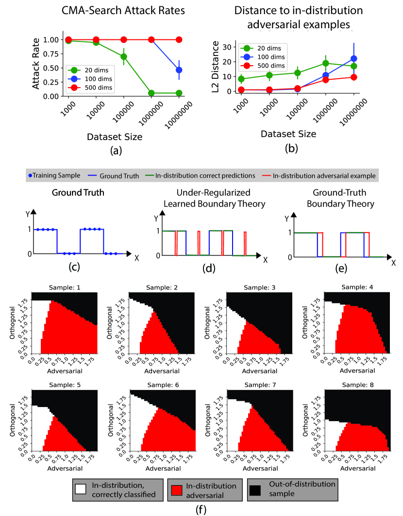
Figure 3: Hypotheses explaining in-distribution adversarial examples. (a) Attack rate of CMA-Search in finding an in-distribution adversarial example starting with a correctly classified sample. Models start becoming robust at high dataset sizes, however the sample complexity scales poorly with data dimensionality. (b) Average Euclidean distance between the starting point and the identified in-distribution adversarial sample. As dataset size increases, the average Euclidean distance from the starting point to in-distribution adversarial example increases for all data dimensions. (c) Example of one-dimensional ground-truth function (d) Depiction of under-regularization learned boundary theory (e) Depiction of ground-truth boundary theory (f) Church window plots depicting adversarial examples in the vicinity of category boundaries.

We build on the same setup as previous work (gilmer2018relationship, )—binary classification of data sampled from two high-dimensional, disjoint uniform distributions (see methods Sec. 4.1). This previous work relied on Projected Gradient Descent to find adversarial examples (fawzi2018adversarial, ; stutz2019disentangling, ), but this approach only works at high dimensions ($>60$) (gilmer2018relationship, ). We present results using our evolutionary strategies based CMA-Search, as it can also find in-distribution adversarial examples in low dimensions as shown in the following. More details on the implementation of CMA-Search are provided in methods Sec. 4.5.

In Fig. 3(d), we report our method’s attack rate for models with high accuracy ($>0.99$). The attack rate measures the fraction of correctly classified points for which an in-distribution adversarial examples can be found in the vicinity using CMA-Search (see methods Sec. 4.6 for more details). These results demonstrate that despite a near perfect accuracy on a held-out, randomly sampled test set, in-distribution adversarial examples can be identified in the vicinity of all correctly classified test points using CMA-Search. This simplistic dataset is easily separable by most conventional machine learning models including a decision tree, which makes the presence of in-distribution adversarial examples both surprising and highly concerning.

In Fig. 3(a) we report the attack rate for models trained with $20$, $100$ and $500$ dimensional data. As can be seen, the attack rate of CMA-Search is nearly $1.0$ till a very large dataset size. However, once a critical dataset size is reached, networks do start becoming robust. Unfortunately, the data complexity scales poorly with number of dimensions. While dimensionality grows five-fold from $20$ to $100$, the number of points required for robustness scales almost 100-fold. Furthermore, for $500$ dimensions we were unable to identify the dataset size required for models to become robust despite trying $10$ million training data points.

In Fig. 3(b) we report the average distance between the (correctly classified) start point and the in-distribution adversarial example. As can be seen, this distance increases as dataset size is increased. As critical dataset size is reached, adversarial examples are far enough from starting points that they are now not in-distribution. This results in a dip in the attack rate, as we only measure in-distribution adversarial examples. This suggests that for a fixed data dimensionality sample complexity does have a significant impact on in-distribution robustness.

We also investigated the role of robust training on in-distribution robustness by including $20,000$ identified adversarial examples alongside $100,000$ training data points and retraining the model for the $100$ dimensional case. We found that the attack rate continued to be $1.0$, with no improvement in model robustness against CMA-Search. This is expected behaviour, as our identified adversarial examples lie within the training distribution, and robust training in this case essentially amounts to a marginal increase in the training dataset size.

Table 1: Role of stochasticity in in-distribution robustness. To isolate the source of high variance in model robustness at high dataset sizes, we investigate four sources of stochasticity one at a time holding other factors constant. These include—inherent stochasticity of CMA-Search, SGD, sampling bias, and model initialization. Our results show that this variance is largely driven by model robustness, which has substantial impact on model robustness.

Stochastic source varied	Attack Rate
CMA-Search	$0.14\pm 0.16$
SGD	$0.22\pm 0.09$
Sampling Bias	$0.08\pm 0.06$
Model Initialization	$0.99\pm 0.03$

While models start becoming robust at high dataset sizes (Fig. 3(a),(b)), we found significant variance in this behaviour. Empirically, we found that the attack rates of models trained at high dataset sizes can also be high at times. This variance is also visible in the error bars in Fig. 3(a),(b). This result suggests that despite the same problem setup some models turn out to be robust, while others do not. To identify the underlying cause of this stochasticity in model robustness, we investigate how robustness changes as a function of four sources of stochasticity—inherent stochasticity of CMA-Search, optimization (SGD), sampling bias, and model initialization. For this analysis, we started by first identifying a robust model trained with $100,000$ points for $20$-dimensional data and then attacked the model again holding everything constant while varying one source of stochasticity at a time.

Results are reported in Table 1. The mean attack rate remains low across multiple CMA-Search repetitions ($0.14$), and across multiple models trained from scratch ($0.22$). Thus, robustness is not due to the inherent stochasticity of CMA-Search, or SGD. Furthermore, new models trained with newly sampled data also resulted in a robust model with a low attack rate of $0.08$, suggesting there is no good dataset which led to the models becoming robust. Interestingly, we find that models trained with new initializations are now non-robust and have a high attack rate of $0.99$. Thus, what makes certain models robust and others non-robust depends on the model initialization. More details on these experiments are provided in Sec. 4.6.3.

In summary, results in Fig. 3 and Table 1 together suggest that while there is widespread presence of adversarial examples within the training distribution, models can start becoming robust at critical (extremely large) dataset sizes. Furthermore, the deciding factor for which models will be robust at extreme sizes is strongly dependent on the model initialization.

Despite evidence supporting the presence of adversarial examples lying within the training distribution, the mechanisms driving such examples remain unknown. There are two main potential hypotheses that can explain such in-distribution adversarial examples. Fig. 3(c) depicts the ground truth function as a one dimensional binary step function for ease of visualization. Firstly, adversarial examples could be an outcome of the learned function being poorly regularized. We call this hypothesis under-regularized learned boundary, and depict it in Fig. 3(d) in one dimension. As can be seen, adversarial examples are spread across the entire range of inputs in this case. For such examples, better regularization can prevent ‘spikes’ in the predicted output and would lead to better in-distribution robustness. Secondly, in-distribution adversarial examples may be an outcome of the complexity of ground-truth boundaries at high dimensions. We call it the ground-truth boundary theory, and depict it in Fig. 3(e) in low dimensions for ease of comprehension. In this case, there are no high-frequency ‘spikes’ in the learned function. Instead, the learned function is simply wrong in estimating where the step function changes from $1$ to $0$ as the probability of sampling near the ground-truth boundary in the training data is infinitesimally small due to the training data being finite. In this case all errors are located in the vicinity of the function transition and better regularization would not help prevent these errors. As shown in previous works investigating this hypothesis (gilmer2018relationship, ; fawzi2018adversarial, ; shafahi2018adversarial, ; mahloujifar2019curse, ; diochnos2018adversarial, ; dohmatob2018limitations, ), the number of function transitions increases combinatorially with dimensionality, making it easier to find an in-distribution adversarial example in the vicinity of one of these transitions. Below, we assess these two hypotheses.

To investigate which of the two hypotheses presented in Fig. 3 hold true for this dataset, we visualize the learned decision boundary in the vicinity of the category transition using church window plots (warde201611, ). More details on how these are plotted is provided in methods Sec. 4.6.2. As can be seen in Fig. 3(f), there is a clean transition from correctly classified points (white) to in-distribution adversarial examples near the decision boundary (red), beyond which points become out of the distribution of samples belonging to a particular category (black). We observed this same behaviour across all church window plots made with multiple randomized samples and orthogonal vectors. In-distibution adversarial examples are isolated to a region close to the category boundary, and in a contiguous fashion. This strongly suggests that these in-distribution adversarial examples occur due to the mechanism presented in Fig. 3(e)—due to ground-truth boundary complexity in high dimensions, as opposed to poor regularization.

2.2 Widespread presence of in-distribution adversarial examples through subtle changes in 3D perspective and lighting

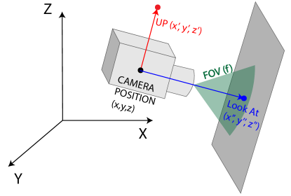
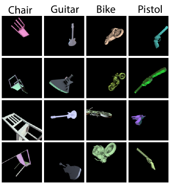
(a)	(b)

Figure 4: 3D scene setup and resulting images. (a) Images in our dataset are completely parametrized by the camera and light. Physical interpretation of the camera parameters is illustrated here. Analogously, light is parametrized by the position, look at, 2D size and the RGB intensities. (b) Sample images for 4 object categories generated using our 3D scene setup. As can be seen, images contain complex viewpoints and locations, multiple colors per object and complex artifacts like self-shadows.

We extend our investigations to parametric and controlled images of objects using our graphics pipeline. We use a computer graphics pipeline for generating and modifying images which ensures complete parametric control over the data distribution. Every image generated from our pipeline can be completely described by their lighting and camera parameters shown in Fig 4(a). To create a dataset with a fixed, known training distribution, we simply sample camera and lighting parameters from a fixed, uniform distribution, and render a subset of 3D models from ShapeNet chang2015shapenet objects with these camera and lighting parameters.

Using this approach, we create a large-scale ($\sim 0.5$ million images) and unbiased dataset of complex image data with a fixed, known distribution. Furthermore, sampling new points from this distribution is as simple as sampling more camera and light parameters from their known distribution. Our pipeline builds upon recent work by Li et al. (li2018differentiable, ). Fig. 4(b) shows sample images sampled from the known training distribution (additional examples from the dataset can be found in Fig. S1). As can be seen, this dataset contains objects seen across multiple viewpoints, scales, and shifted across the frame. Furthermore, we use physically based rendering li2018differentiable ; pharr2016physically to accurately simulate complex lighting artifacts including diverse lighting conditions like multiple colors and self-shadows which makes the dataset challenging for neural networks. We ensure that the following constraints are met: (1) uniformly distributed and unbiased training data, (2) $1000$ images per 3D object (total $0.5$ million images), and (3) no spurious correlations between the scene parameters and the image labels. More details on dataset generation can be found in methods Sec. 4.2.

We first investigate how well object recognition models perform across camera and lighting variations while ensuring an exact match between training and testing distributions. Both the train and the test sets are created by sampling uniformly across the range of camera and lighting parameters for this experiment. We evaluate both Convolutional Neural Networks (CNNs) and transformer-based models. Exact hyper-parameters and other details on model training are provided in methods Sec. 4.4

The difficulty in classifying these images is corroborated in Table 2, as there is significant room for improvement for both CNNs and transformer-based models. Table 2 reports accuracy for several state-of-the-art CNNs he2016deep ; zhang2019making ; chaman2020truly and transformer architectures including the vision transformer (ViT) dosovitskiy2020image , and the data efficient transformer (DeIT) and its distilled version (DeIT Distilled) touvron2020deit . As can be seen, neural networks do not perform very well across camera and lighting variations. In fact, the problem is even more pronounced with transformer models. To test if this problem can be mitigated with shift-invariant architectures, we also report results on two specialized shift-invariant architectures - Anti-Aliased Networks zhang2019making , and the recent Truly Shift Invariant Network chaman2020truly . While these networks do provide a boost in performance, they too are susceptible to camera and lighting variations. We also confirm that this is not an outcome of our neural networks overfitting by testing the network on new, unseen 3D models. The performance on these new 3D models also mirrors the same trend, as seen in Table 2.

Table 2: Performance of object recognition models on seen and new 3D models.

Accuracy	ResNet	ResNet (pretrained)	Anti-Aliased Networks	Truly Shift Invariant	ViT	DeIT	DeIT Distilled
Seen models	0.75	0.76	0.82	0.80	0.58	0.63	0.64
New models	0.70	0.70	0.74	0.72	0.59	0.64	0.65

These results naturally raise the question—What images are these networks failing on? Are there certain lighting and camera conditions that the networks fail on? The one-to-one mapping between the pixel space (images) and our low-dimensional scene representation (i.e. camera and lighting parameters) allows us to answer these questions by visualizing and comparing correctly and incorrectly classified images in this low dimensional space. In Fig. 5 we show the distribution of camera parameters for images which were classified incorrectly. As can be seen, the errors seem well distributed across space—we found no clear, strong patterns which characterize the camera and light conditions of misclassified images. Note that regions in each of these parametric spaces represent human interpretable scenarios which have been known to impact human vision significantly. For instance, changes in camera position represent canonical vs non-canonical poses which significantly impact human vision gomez2008memory ; terhune2005recognition ; blanz1999object . Similarly, changes in the up vector can represent upside-down objects which too impact human vision kohler1960dynamics ; lewis2001lady ; thompson1980margaret . In contrast, Fig. 5 shows that networks do not suffer in specific regions of the space. These results are consistent across multiple architectures. Supplemental Fig. S2 shows examples of this phenomenon multiple object categories and neural network architectures.

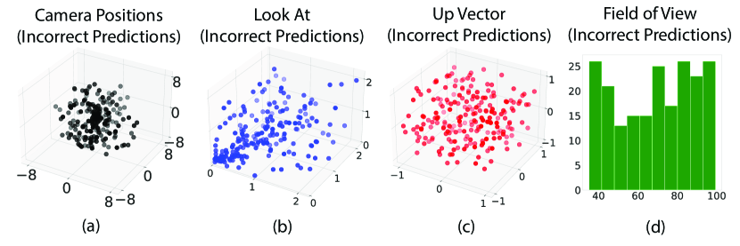
Figure 5: Distribution of errors across the scene parameter space. (a) Coordinates of camera positions, (b) Coordinates of Look At, (c) Up Vector and (d) Histogram of errors across lens field of view (FOV). We found no clear, strong patterns which characterize the camera and light conditions of misclassified images. This is in contrast to human vision which is impacted by regions of camera positions (non-canonical viewpoints), and up vector (upside-down orientations) among others.

Table 3: CMA-Search over camera and light parameters. Starting with new, correctly classified in-distribution images, we use our method to search the vicinity of camera and light positions, starting with the original image’s parameters. Attack Rate reports the percentage of times an in-distribution adversarial example was found starting with a correctly classified image. We also report the mean and standard deviation of the distance between the original image and the identified in-distribution adversarial example. This distance is measured by calculating the L2 distance between the camera parameters of the original correctly classified image and the parameters of the in-distribution adversarial example in its vicinity, and normalizing it by the range of the camera parameters.

Model Architecture	CMA Cam		CMA Light
	Attack Rate (%)	Distance (mean $\pm$ std)	Attack Rate (%)	Distance (mean $\pm$ std)
ResNet18 he2016deep	71	1.83 $\pm$ 1.33	42	6.52 $\pm$ 5.68
ResNet18 (pretrained) he2016deep	58	1.79 $\pm$ 1.46	36	5.36 $\pm$ 3.70
Anti-Aliased Networks zhang2019making	45	2.32 $\pm$ 2.09	40	7.03 $\pm$ 5.10
Truly Shift Invariant Network chaman2020truly	53	2.22 $\pm$ 2.16	25	6.72 $\pm$ 5.41
ViT dosovitskiy2020image	85	1.34 $\pm$ 1.16	65	4.63 $\pm$ 3.49
DeIT touvron2020deit	85	1.27 $\pm$ 0.81	51	4.54 $\pm$ 2.75
DeIT Distilled touvron2020deit	86	1.22 $\pm$ 0.87	55	4.49 $\pm$ 2.27

While above results prove the existence of adversarial examples within the training distribution, a key requirement for such examples is the imperceptibility of the change needed to introduce an error. To introduce such imperceptible changes, we propose an evolution-strategies based error search methodology for in-distribution, misclassified images which we call CMA-Search. Starting with a correctly classified image, our method searches within in the vicinity of the camera and lighting parameters to find an in-distribution image which is incorrectly classified. Note that unlike adversarial attacks, our method does not add noise and our constraints ensure that identified errors are in-distribution. CMA-search enables interpretable attacks by searching over the scene’s camera and light parameters, while only sampling from within the training distribution. For instance, it is possible to attack a model by searching over solely the camera position ($3$ dimensions), while holding all other scene parameters constant. While previous works have attempted to find in-distribution adversarial examples by approximating the data distribution using generative models (stutz2019disentangling, ; fawzi2018adversarial, ), we provide first empirical evidence for in-distribution adversarial examples in object recognition.

As shown in Table 3, CMA-Search finds small changes in 3D perspective and lighting which have a drastic impact on network performance. For example, starting with an image correctly classified by a ResNet18 he2016deep model, our method can find an error in its vicinity for $71\%$ cases with an average change of $1.83\%$ in the camera position. For transformers, the impact is far worse, with an attack rate of $85\%$. Similarly, with lighting changes CMA-Search can find a misclassification in $42\%$ cases with an average change of $6.52\%$ for a ResNet18 model. These results are reported for various architectures in Table 3. As can be seen, we find that networks are most sensitive to changes in the Camera Position and the camera Look At—subtle, in-distribution 3D perspective changes. This behaviour is consistent across several architectures. In fact, even shift-invariant architectures specifically designed to be robust to 2D shifts are still highly susceptible to 3D perspective changes.

Thus, the space of camera and lighting variations is filled with in-distribution adversarial examples in the vicinity of correctly classified points. Unfortunately, church-window plots similar to Fig. 3 cannot be replicated for complex image data as the transition boundary between two object categories is hard to define. However, our results provide evidence in support of the ground-truth boundary theory as an explanation for adversarial examples in object recognition, and calls into question existing theories which attribute adversarial examples to systematic differences in the training and test distributions.

2.3 Approximate in-distribution adversarial examples in the vicinity of natural images

So far, our experiments have focused on datasets with complete control over the training distribution. Here, we present results on approximate in-distribution adversarial examples for natural images taken from the ImageNet dataset deng2009imagenet . Specifically, we used CMA-Search to optimize the camera parameters, but instead of our renderer, we now use a novel view synthesis model (MPI tucker2020single ) for generating novel views of ImageNet images. More details on this procedure can be found in methods Sec. 4.3.

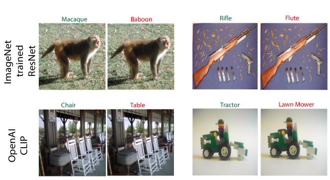
Figure 6: CMA-Search on ImageNet images. To replicate results on ImageNet, we replace our rendering pipeline with the single view MPI tucker2020single model to generate novel views of ImageNet images. Here we show results using CMA-Search with the MPI model to find subtle 3D perspective changes which lead to misclassification with ResNet18 and OpenAI’s CLIP model.

Starting with a correctly predicted ImageNet image, we use CMA-Search in conjunction with the MPI model to find images in the vicinity with small, 3D perspective changes which can break ImageNet trained classification networks including ResNet18, and OpenAI’s transformer based CLIP model radford2021learning . Results for these experiments are reported in Fig. 6. We provide additional examples of misclassified ImageNet images found using CMA-Search in Supplementary Fig. S3. MPI model was not trained on ImageNet, and can at times fail to generate novel views, resulting in blurry images instead. We omit these images to only present results on adversarial examples due to small, 3D perspective changes. While these results present an interesting application on natural images, these results are only approximately in-distribution like previous works that also explored in-distriubtion adversarial examples (stutz2019disentangling, ; fawzi2018adversarial, ). We cannot be entirely sure that the images found by CMA-Search on ImageNet are indeed in-distribution, further justifying the necessity of our computer graphics based approach in the previous section.

3 Discussion

Recent theoretical works developing the ground-truth boundary theory have investigated adversarial examples within the training data distribution. This added constraint requiring adversarial examples be in-distribution results in a more stringent definition of adversarial examples, which presents an opportunity to further scrutinize and update existing theories on the origin of adversarial examples. However, these works were restricted to simplistic, parametrically controlled data. Here we provided evidence that these in-distribution adversarial examples extend to images of objects. These results provide new, stronger evidence in support of the ground-truth boundary theory being the primary mechanism driving in-distribution adversarial examples.

In practice, the presence of these examples points to a highly worrisome problem—it bypasses the need for a malicious agent to add engineered noise to induce an error. These examples lie hidden within the data distribution in plain sight. In fact, our results show that the problem runs far deeper than previously thought as it is even possible to attack models trained on as low as 5-dimensional data.

We also show that the current best practices for adversarial defense are insufficient to address in-distribution adversarial examples. Most existing approaches revolve around the idea of robust training madry2017towards , i.e. including adversarial examples into the training set. As mentioned in Sec. 2.1, we confirmed that in-distribution errors could not be removed by robust training. This may be because finding adversarial examples is computationally costly and models start becoming robust only at extreme dataset sizes, and that this critical size increases exponentially with data dimensionality. This need for extreme dataset size can be explained by the ground-truth boundary theory. There is combinatorial increase in the number of ground-truth boundary transitions as data dimensionality increases, and thus a corresponding drop in the probability of a randomly sampled point being sufficiently close to the transition boundary as explained in Fig. 3. In this way, an increasingly large number of samples are needed to obtain samples from the boundary transitions as dimensionality increases. Recent work on scaling laws pmlr-v162-bansal22b ; kaplan2020scaling has investigated accuracy at extreme dataset sizes, but our finding suggests similar scaling laws could also be identified for model robustness.

Based on our findings, we propose three potential directions which might help alleviate in-distribution adversarial examples. Firstly, reducing the data representation dimensionality. As dataset size needed for robustness scales poorly with dimensions, efficient dimensionality reduction on data representation may help reduce samples needed to train a robust model. Secondly, better model initialization. We showed that once critical dataset size is reached, model robustness strongly depends on initialization, and thus future researchers may need to devise better initialization techniques which result in more robust models. Thirdly, casting object recognition as a smooth regression problem that reduces the number of ground-truth boundary transitions as these examples are located only in the vicinity of these boundaries (Fig. 3).

In summary, we have provided empirical evidence of the widespread presence of in-distribution adversarial examples for complex image data, which is highly worrisome and has concerning ramifications for the origin of and defense against adversarial examples. Going forward, we hope that future researchers can combine theoretical and empirical investigations using the unified framework provided in our work, and help move the machine learning and computer vision communities closer to a deeper understanding of the phenomenon we call adversarial examples. Understanding these susceptibilities of object recognition models lies at the heart of building robust and reliably deployable models, and we hope this research direction can make a strong contribution towards this end.

4 Methods

4.1 Generating simplistic parametrically controlled data

We created a binary classification task by sampling data from two $N$-dimensional uniform distributions confined to disjoint ranges $(a,b)$ and $(c,d)$, as described in the following:

$$x_{i}\sim\left\{\begin{array}[]{lr}\text{Unif}(a,b,N);&y_{i}=0\\ \text{Unif}(c,d,N);&y_{i}=1\end{array}\right\}.$$ (1)

We set $a=-10,b=10,c=20,d=40$ for experiments presented in Sec. 2.1. However, we observed that the exact choice of these parameters does not impact our findings. To measure in-distribution performance, we simply sample new data points from these same distributions.

4.2 Generating controlled rendered data of real world objects

Most large-scale datasets for computer vision have been created by scraping pictures from the internet deng2009imagenet ; lin2014microsoft ; pascal-voc-2012 ; KrauseStarkDengFei-Fei_3DRR2013 ; zhou2017places . For experiments investigating in-distribution robustness, these datasets present two major challenges. Firstly, it is not possible to quantitatively define or control the distribution of these datasets in closed form. Secondly, investigating in-distribution robustness requires being able to sample new points from regions of interest within the data distribution, and to test model performance on these samples. This is not possible with internet scraped datasets. These problems have inspired the growing trend of research works using carefully designed synthetic data with controlled data distributions qiu2016unrealcv ; hendrycks2019benchmarking ; madan2020capability ; bomatter2021pigs ; leclerc2021three ; wang2021advsim . In a similar vein, our graphics pipeline (explained below) easily allows us to generate a large-scale, unbiased dataset of objects seen under varied camera and lighting conditions with complete control over the data distribution. Sample images from four categories are shown in Fig. 4(b). Each 3D model was rendered under 1000 different camera and lighting conditions following the scene setup described below. Fig. S1 shows additional sample images from the dataset. Below we introduce the 3D scene setup, camera and lighting parameter sampling strategies, and the 3D models used to generate our dataset.

4.2.1 3D Scene Setup

All rendering was done using the open-source rendering pipeline Redner li2018differentiable . Each scene contains one camera, one 3D model and 1-4 lights. To ensure there are no spurious correlations between object category, texture and background geirhos2018imagenet , the texture for all ShapeNet chang2015shapenet objects was replaced with a simple diffuse material and the background was kept constant. Thus, every scene is completely parametrized by the camera and the light parameters. As shown in Fig. 4(a), camera parameters are 10 dimensional: one dimension for the FOV (field of view of camera lens), and three dimensions each for the Camera Position (coordinates of camera center), Look At (point on the canvas where the camera looks), and the UP vector (rotation of camera). Analogously, lights are represented by 11 dimensions - two dimensions for the Light Size, and three each for Light Position, light Look At and RGB color intensity. Multiple lights ensure that scenes contain complex lighting scenarios including multiple colors and self-shadows. Thus, our scenes are $(11n+10)$ dimensional, where $n$ is the number of lights. There is a one-to-one mapping between the pixel space (rendered images) and this low dimensional scene representation.

4.2.2 Unbiased, uniform sampling of scene parameters

To ensure an unbiased distribution over different viewpoints, locations on the frame, perspective projections and colors, we ensured that scene parameters follow a uniform distribution. Concretely, camera and light positions were sampled from a uniform distribution on a spherical shell with a fixed minimum and maximum radius. The Up Vector was uniformly distributed across range of all possible camera rotations, and RGB light intensities were uniformly distributed across all possible colors. Camera and light Look At positions were uniformly distributed while ensuring the object stays in frame and is well-lit (frame size depends on Camera Position and FOV). Finally, Light Size and camera FOV were uniformly sampled 2D and 1D vectors. Below we specify the hyper-parameters for rendering, along with the exact distribution for each scene parameter and the corresponding sampling technique used to sample from these distributions.

Camera Position: For scene camera, first a random radius $r_{c}$ is sampled while ensuring $r_{c}\sim$ Unif$(0.5,8)$. Then, the camera is placed on a random point denoted $(x_{c},y_{c},z_{c})$ on the spherical shell of radius $r_{c}$. To generate a random point on the sphere while ensuring an equal probability of all points, we rely on the method which sums three randomly sampled normal distributions harman2010decompositional :

$$X,Y,Z\sim\mathcal{N}(0,1),$$ (2)

$$v=(X,Y,Z),$$ (3)

$$(x_{c},y_{c},z_{c})=r_{c}*\frac{v}{\|v\|}.$$ (4)

Camera Look At: To ensure the object is shown at different locations within the camera frame, the camera Look At needs to be varied. However, range of values such that the object is visible can be present across the entire range of the frame depends on the camera position. So, we sample camera Look At as $l_{c}$ as follows:

$$l_{c}\sim\text{Unif}(K*x_{c},K*y_{c},K*z_{c}),\text{where }K=0.3.$$ (5)

The value $K=0.3$ was found empirically. We found it helped ensure that objects show up across the whole frame while still being completely visible within the frame.

Camera Up Vector: Note that the camera Up Vector is implemented as the vector joining the camera center (0,0,0) to a specified position. We sample this position and therefore the Up Vector $u_{c}$ as follows:

$$x,y,z\sim\text{Unif}(-1,1),$$ (6)

$$u_{c}=(x,y,z).$$ (7)

Camera Field of View (FOV): We sample the field of view $f_{c}$ while ensuring:

$$f_{c}\sim\text{Unif}(K_{1},K_{2}).$$ (8)

Again, the values $K_{1}=35,K_{2}=100$ were found empirically to ensure objects are completely visible within the frame while not being too small.

Light Position: For every scene we first sample the number of lights $n$ between 1-4 with equal probability. For each light $i$, a random radius $r_{i}$ is sampled ensuring $r_{i}\sim\text{Unif}(R_{1},R_{2})$, then the light is placed on a random point $(x_{i},y_{i},z_{i})$ on the sphere of radius $r_{i}$. $R_{1}=1$ and $R_{2}=8$ were found empirically to ensure that the light is able to illuminate the 3D model appropriately.

Light Look At: To ensure that the light is visible on the canvas, light Look At is sampled as a function of the camera position:

$$l_{i}\sim\text{Unif}(K*x_{c},K*y_{c},K*z_{c}),\text{where }K=0.3.$$ (9)

As in the case of the Camera Look At parameter mentioned above, the value $K=0.3$ was found empirically.

Light Size: Every light in our setup is implemented as an area light, and therefore requires a height and width to specify the size. We generate the size $s_{i}$ for light $i$ as:

$$h,w\sim\text{Unif}(L_{1},L_{2}),$$ (10)

$$s_{i}=(h,w).$$ (11)

$L_{1}=0.1,L_{2}=5$ were found empirically to ensure the light illuminates the objects appropriately.

Light Intensity: This parameter specifies the RGB intensity of the light. For light $i$, RGB color intensity $c_{i}$ was sampled as:

$$r,g,b\sim\text{Unif}(0,1),$$ (12)

$$c_{i}=(r,g,b).$$ (13)

Object Material: To ensure no spurious correlations between object texture and category, all object textures were set to a single diffuse material. Specifically, the material is a linear blend between a Lambertian model and a microfacet model with Phong distribution, with Schilick’s Fresnel approximation. Diffuse reflectance was set to 1.0, and the material was set to reflect on both sides.

4.2.3 3D models used for generating two different test sets

Our dataset contains 11 categories, with 40 3D models for every category chosen from ShapeNet chang2015shapenet . Neural networks were evaluated on two test sets - one with the 3D models seen during training, and the second with new, unseen 3D models. The first test set was generated by simply repeating the same procedure as described above. Thus, the  (Geometry $\times$ Camera $\times$ Lighting) joint distribution matches exactly for the train set and this test set. The second test set was created by the exact same generation procedure, but with 10 new 3D models for every category chosen from ShapeNet. The motivation for this second test set was to ensure our models are not over-fitting to the 3D models used for training. Thus, the  (Camera $\times$ Lighting) joint distribution matches exactly for this test set and the train set, but the Geometry is different in these two sets.

4.3 Generating natural images in the vicinity of ImageNet images

One of the major challenges in extending our results to natural image datasets is generating natural images in the vicinity of a correctly classified image by slightly modifying the camera parameters. To do so for ImageNet is equivalent to novel view synthesis (NVS) from single images, which has been a long standing challenging task in computer vision. However, recent advances in NVS enable us to extend our method to natural image datasets like ImageNet yoon2020novel ; zhou2016view ; wiles2020synsin ; tucker2020single .

To generate new views in the vicinity of ImageNet images, we rely on a single-view synthesis model based on multi-plane images (MPI) tucker2020single . The MPI model takes as input an image and the $(x,y,z)$ offsets which describe camera movement along the X, Y and Z axes. Note that unlike our renderer, it cannot introduce changes to the camera Look At, Up Vector, Field of View or lighting changes.

4.4 Model Training Details

Below we provide the training details including model architectures, optimization strategies and other hyper-parameters used for the binary classification models trained on simplistic parametrically controlled data, and the object recognition models trained on our rendered images of camera and light variations.

4.4.1 MLPs for classifying parametrically controlled uniform data

Let $D$ denote the dimensionality of the input data, and $N$ denote the total number of data points. We used a $5$ layer multi-layer perceptron (MLP) with ReLU activations, with the output dimensionality of layers set to $5D$, $D$, $D/5$, $D/5$, and $2$ respectively. However, we found that the number of MLP hidden layers and the number of neurons in these layers had no impact on trends of in-distribution robustness. For experiments with $N<64,000$ all data was passed in a single batch. For experiments with more data points, each batch contained $64,000$ points. All models were trained for $100$ epochs with stochastic gradient descent (SGD) with a learning rate of $0.0001$. All experiments were conducted on a compute cluster consisting of 8 NVIDIA TeslaK80 GPUs, and all models were trained on a single GPU at a time. Only models achieving a near perfect accuracy ($>0.99$) on a held-out test set were attacked using CMA-Search.

4.4.2 Object recognition models for classifying images of real-world objects

All CNN models were trained with a batch size of 75 images, while transformers were trained with a batch size of 25. Models were trained for $50$ epochs with an Adam optimizer with a fixed learning rate of 0.0003. Other learning rates including 0.0001, 0.001, 0.01 and 0.1 were tried but they performed either similarly well or worse. To get good generalization to unseen 3D models and stable learning, each image was normalized to zero mean and unit standard deviation. As before, all experiments were conducted on our cluster with TeslaK80 GPUs, and each model was trained using a single GPU at a time.

4.5 CMA-Search: Finding in-distribution adversarial examples by searching the vicinity

To investigate the in-distribution robustness of neural networks with respect to changes in camera and lighting, we propose a new, gradient-free search method to find incorrectly classified images. Starting with a correctly classified image, our method searches the vicinity by slightly modifying camera or light parameters to find an in-distribution error. While adversarial viewpoints and lighting have been reported before in the literature liu2018beyond ; zeng2019adversarial ; jain2019generating , there are two major differences in our approach. First, these methods search for an adversarial image by adding a perturbation to the input scene parameter without constraining the resulting image to be within the training distribution. In comparison, our approach searches within the distribution to find in-distribution errors. Secondly, unlike our gradient-free search method, these methods often rely on gradient descent and thus require high dimensional representations of the scene to work well. For instance, these works often use neural rendering where network activations act as a high dimensional representation of the scene zeng2019adversarial ; joshi2019semantic , or use up-sampling of meshes to increase dimensionality liu2018beyond .

Algorithm 1 CMA-Search over camera parameters to find in-distribution adversarial examples.

1:Let $x\in\mathbb{R}^{10}$ denote the camera parameters.

2:Let Render and Network denote the rendering pipeline and classification network respectively.

3:function Fitness($x$, Render, Network)

4:     image = Render$(x)$

5:     predicted_category, probability = Network$($image$)$

6:     return predicted_category, probability

7:

8:Let $x_{init}$ denote initial camera parameters, $\lambda$ be number of offspring per generation, and $y$ be the image category.

9:

10:procedure CMA-Search($x_{init},\lambda,y$)

11:     initialize $\mu=x_{init},C=I$ $\triangleright$ $I$ denotes identity matrix.

12:     while True do

13:         for j = $1,...,\lambda$ do

14:              $x_{j}=$ sample_multivariate_normal($\mu,C$) $\triangleright$ Generate mutated offspring

15:              $y_{j},p_{j}=$FITNESS($x_{j}$, Render, Network) $\triangleright$ Calculate fitness of offspring

16:              if $y_{j}\neq y$ then

17:                  return $x_{j}$ $\triangleright$ Classification fails for image with camera parameters $x_{j}$                        

18:         $x_{1...\lambda}\leftarrow x_{s(1)...s(\lambda)}$, with $s(j)$ = argsort($p_{j}$) $\triangleright$ Pick best offspring

19:         $\mu,C\leftarrow$ update_parameters($x_{1...\lambda},\mu,C$)      

We extend these approaches to work well with our low-dimensional scene representation by utilizing a gradient-free optimization method to search the space—Covariance Matrix Adaptation-Evolution Strategy (CMA-ES) hansen1996adapting ; hansen2016cma . We found that gradient descent with differentiable rendering struggled to find in-distribution errors in our scenes due to the low dimensionality of the optimization problem. CMA-ES has been found to work reliably well with non-smooth optimization problems and especially with local optimization hansen2001completely , which made it a perfect fit for our search strategy. In contrast to gradient based methods requiring high dimensions, our approach works well for as low as 3 dimensions.

Algorithm 2 provides an outline of using CMA-Search to find in-distribution adversarial examples by searching the vicinity of camera parameters. The algorithm for searching for adversarial examples using light parameters in rendered data, and within parametrically controlled unifrom data is analogous. In Fig. 2 we show examples of in-distribution adversarial examples found by our CMA-Search method over camera parameters. Starting with the correctly classified image (left), our method finds an image in the vicinity by slightly modifying camera parameters of the scene. As can be seen, subtle changes in 3D perspective can lead to drastic errors in classification. We also highlight the subtle changes in camera position (in black) and camera Look At (in blue) in the figure. To the best of our knowledge, this is the first evolutionary strategies based search method for finding in-distribution adversarial examples.

Starting from the initial parameters, CMA-ES generates offspring by sampling from a multivariate normal (MVN) distribution i.e. mutating the original parameters. These offspring are then sorted based on the fitness function (classification probability), and the best ones are used to modify the mean and covariance matrix of the MVN for the next generation. The mean represents the current best estimate of the solution i.e. the maximum likelihood solution, while the covariance matrix dictates the direction in which the population should be directed in the next generation. The search is stopped either when a misclassification occurs, or after 15 iterations over scene parameters. For the simplistic parametrically controlled data, we check for a misclassification till 1500 iterations. More details on the exact subroutines for parameter update and theoretical underpinnings of the CMA-ES algorithm can be found in the documentation for pycma hansen2019pycma and the accompanying paper hansen2016cma .

4.6 Evaluation details

Below we provide details on the evaluation and visualization of in-distribution adversarial examples identified by CMA-Search.

4.6.1 Evaluating CMA-Search using the Attack Rate

To quantify the performance of CMA-Search and the prevalence of in-distribution adversarial examples we propose the Attack Rate, which is reported in Tables  1 and  3. For the simplistic parametrically controlled data, we first randomly sample $1000$ test points which we confirm are correctly classified by the classification model. For each of these test points, CMA-Search is then tasked with starting from the correctly classified point and searching for a nearby point within the training data distribution where the classifier fails. The Attack Rate is the fraction of these $1000$ correctly classified points for which CMA-Search is able find an in-distribution adversarial example in the vicinity. This process is repeated $10$ times and the average value is reported. For image data, sampling a new point involves sampling scene parameters and rendering the new image corresponding to these parameters. As rendering is significantly slower, we measure the attack rate using $20$ samples for image data, and report average over $10$ repeats.

4.6.2 Church-window plots

CMA-Search starts from a correctly classified point and provides an in-distribution adversarial example. We use this to define a unit vector in the adversarial direction, and fix this as one of basis vectors for the subspace the data occupies. Assuming data dimensionality to be $D$, we can calculate the corresponding $D-1$ orthonormal bases. Following the same protocol as past work warde201611 , we randomly pick one of these orthonormal vectors as the orthogonal direction and define a grid of perturbations with fixed increments along the adversarial and the orthogonal directions. These perturbations are then added to the original sample and the model is evaluated at these perturbed samples. We plot correct classifications in white, in-distribution adversarial examples in red, and out-of-distribution samples in black.

4.6.3 Sources of stochasticity

Table 1 reports the results of Attack Rates for models as sources of stochasticity are varied one at a time to investigate their impact on model robustness. For these experiments, we studied binary classification models trained on $100,000$ data points of $20$-dimensional data. Below, we provide additional details on how these experiments were conducted.

CMA-Search: As our method is based on evolutionary strategies, it is inherently stochastic. To ensure that model robustness is not due to CMA-Search failing stochastically, we repeat the attack on our robust model with CMA-Search 10 times and report the mean attack rates.

Optimization (SGD): To investigate if the optimization process enables certain models to be robust, we use the exact same data points and model initialization as the identified robust model, and repeat the training procedure 10 times to obtain 10 different models. These models differ from each other only due to the stochasticity of SGD.

Sampling Bias: We ask if model robustness is a function of the specific training data sampled from the training distribution - is there a good training dataset that results in more robust models? We test this by using this exact same initialization and SGD seed as the robust model, and train models on newly data sampled from the training distribution. We ensure that the newly sampled dataset has the same size and distribution as the dataset used with the identified robust model.

Model Initialization: To test if the model initialization is the underlying cause for model robustness, we train multiple models with the exact same training data as the robust model, but with different random initialization (different from the robust model) while using the same seed for SGD.

Author contributions statement

SM, XB and TL designed research with contributions of HP; SM performed experiments with contributions of XB and TL; SM and XB wrote the paper with contributions of TL, TS and HP; HP and TS supervised the research.

Data and Code Availability Statement

Source code, data and demos are available on GitHub at https://github.com/Spandan-Madan/in_distribution_adversarial_examples.

Conflict of Interest Statement

This study received funding from Fujitsu Limited. The funder through TS had the following involvement with the study: writing of this article and supervision of the study. All authors declare no other competing interests.

Figure S1: Sample Images from dataset

Figure S2: Camera Parameters that lead to misclassifications for multiple categories and architectures. (a) Camera Position, (b) Camera Look At, (c) Up Vector, (d) Histogram of Lens Field of View.

Figure S3: More examples of misclassified ImageNet-like images discovered by CMA-Search combined with the single view MPI model.

References

- [1] Thomas Tanay and Lewis Griffin. A boundary tilting persepective on the phenomenon of adversarial examples. arXiv preprint, arXiv:1608.07690, 2016.
- [2] Alhussein Fawzi, Seyed-Mohsen Moosavi-Dezfooli, and Pascal Frossard. Robustness of classifiers: from adversarial to random noise. In Advances in Neural Information Processing Systems, volume 29, 2016.
- [3] Adi Shamir, Itay Safran, Eyal Ronen, and Orr Dunkelman. A simple explanation for the existence of adversarial examples with small hamming distance. arXiv preprint, arXiv:1901.10861, 2019.
- [4] Adi Shamir, Odelia Melamed, and Oriel BenShmuel. The dimpled manifold model of adversarial examples in machine learning. arXiv preprint, arXiv:2106.10151, 2021.
- [5] Nicolas Ford, Justin Gilmer, Nicolas Carlini, and Ekin D. Cubuk. Adversarial examples are a natural consequence of test error in noise. In Proceedings of the 36th International Conference on Machine Learning (ICML), pages 2280–2289, 2019.
- [6] Andrew Ilyas, Shibani Santurkar, Dimitris Tsipras, Logan Engstrom, Brandon Tran, and Aleksander Madry. Adversarial examples are not bugs, they are features. In Advances in Neural Information Processing Systems, 2019.
- [7] Dimitris Tsipras, Shibani Santurkar, Logan Engstrom, Alexander Turner, and Aleksander Madry. Robustness may be at odds with accuracy. In Proceedings of the International Conference on Learning Representations (ICLR), 2019.
- [8] Ludwig Schmidt, Shibani Santurkar, Dimitris Tsipras, Kunal Talwar, and Aleksander Madry. Adversarially robust generalization requires more data. In Advances in Neural Information Processing Systems, volume 31, 2018.
- [9] Sébastien Bubeck, Yin Tat Lee, Eric Price, and Ilya Razenshteyn. Adversarial examples from computational constraints. In Proceedings of the International Conference on Machine Learning (ICML), pages 831–840, 2019.
- [10] Preetum Nakkiran. Adversarial robustness may be at odds with simplicity. arXiv preprint, arXiv:1901.00532, 2019.
- [11] Justin Gilmer, Luke Metz, Fartash Faghri, Samuel S Schoenholz, Maithra Raghu, Martin Wattenberg, and Ian Goodfellow. The relationship between high-dimensional geometry and adversarial examples. arXiv preprint, arXiv:1801.02774, 2018.
- [12] Alhussein Fawzi, Hamza Fawzi, and Omar Fawzi. Adversarial vulnerability for any classifier. In Advances in Neural Information Processing Systems, volume 31, 2018.
- [13] Ali Shafahi, W Ronny Huang, Christoph Studer, Soheil Feizi, and Tom Goldstein. Are adversarial examples inevitable? arXiv preprint, arXiv:1809.02104, 2018.
- [14] Saeed Mahloujifar, Dimitrios I Diochnos, and Mohammad Mahmoody. The curse of concentration in robust learning: Evasion and poisoning attacks from concentration of measure. In Proceedings of the AAAI Conference on Artificial Intelligence, volume 33, pages 4536–4543, 2019.
- [15] Dimitrios Diochnos, Saeed Mahloujifar, and Mohammad Mahmoody. Adversarial risk and robustness: General definitions and implications for the uniform distribution. In Advances in Neural Information Processing Systems, volume 31, 2018.
- [16] Elvis Dohmatob. Limitations of adversarial robustness: strong no free lunch theorem. In Proceedings of the 36th International Conference on Machine Learning (ICML), pages 1646–1654, 2019.
- [17] Spandan Madan, Timothy Henry, Jamell Dozier, Helen Ho, Nishchal Bhandari, Tomotake Sasaki, Frédo Durand, Hanspeter Pfister, and Xavier Boix. When and how convolutional neural networks generalize to out-of-distribution category–viewpoint combinations. Nature Machine Intelligence, 4:146 – 153, 2022.
- [18] Gül Varol, Javier Romero, Xavier Martin, Naureen Mahmood, Michael J. Black, Ivan Laptev, and Cordelia Schmid. Learning from synthetic humans. In Proceedings of the IEEE/CVF Conference on Computer Vision and Pattern Recognition (CVPR), 2017.
- [19] Jiteng Mu, Weichao Qiu, Gregory D Hager, and Alan L Yuille. Learning from synthetic animals. In Proceedings of the IEEE/CVF Conference on Computer Vision and Pattern Recognition (CVPR), pages 12386–12395, 2020.
- [20] Xiaohui Zeng, Chenxi Liu, Yu-Siang Wang, Weichao Qiu, Lingxi Xie, Yu-Wing Tai, Chi-Keung Tang, and Alan L Yuille. Adversarial attacks beyond the image space. In Proceedings of the IEEE/CVF Conference on Computer Vision and Pattern Recognition (CVPR), pages 4302–4311, 2019.
- [21] Richard Tucker and Noah Snavely. Single-view view synthesis with multiplane images. In Proceedings of the IEEE/CVF Conference on Computer Vision and Pattern Recognition (CVPR), pages 551–560, 2020.
- [22] Jia Deng, Wei Dong, Richard Socher, Li-Jia Li, Kai Li, and Li Fei-Fei. ImageNet: A large-scale hierarchical image database. In Proceedings of the IEEE Conference on Computer Vision and Pattern Recognition (CVPR), pages 248–255, 2009.
- [23] Alec Radford, Jong Wook Kim, Chris Hallacy, Aditya Ramesh, Gabriel Goh, Sandhini Agarwal, Girish Sastry, Amanda Askell, Pamela Mishkin, Jack Clark, Gretchen Krueger, and Ilya Sutskever. Learning transferable visual models from natural language supervision. In Proceedings of the 38th International Conference on Machine Learning (ICML), pages 8748–8763, 2021.
- [24] David Stutz, Matthias Hein, and Bernt Schiele. Disentangling adversarial robustness and generalization. In Proceedings of the IEEE/CVF Conference on Computer Vision and Pattern Recognition (CVPR), pages 6976–6987, 2019.
- [25] David Warde-Farley and Ian Goodfellow. Adversarial perturbations of deep neural networks. In Tamir Hazan, George Papandreou, and Daniel Tarlow, editors, Perturbations, Optimization, and Statistics, pages 311–342. MIT Press, Cambridge, MA, USA, 2016.
- [26] Angel X. Chang, Thomas Funkhouser, Leonidas Guibas, Pat Hanrahan, Qixing Huang, Zimo Li, Silvio Savarese, Manolis Savva, Shuran Song, Hao Su, Jianxiong Xiao, Li Yi, and Fisher Yu. ShapeNet: An information-rich 3D model repository. Technical Report arXiv:1512.03012 [cs.GR], Stanford University — Princeton University — Toyota Technological Institute at Chicago, 2015.
- [27] Tzu-Mao Li, Miika Aittala, Frédo Durand, and Jaakko Lehtinen. Differentiable Monte Carlo ray tracing through edge sampling. ACM Transactions on Graphics (TOG), 37(6):1–11, 2018.
- [28] Matt Pharr, Wenzel Jakob, and Greg Humphreys. Physically based rendering: From theory to implementation. Morgan Kaufmann, 2016.
- [29] Kaiming He, Xiangyu Zhang, Shaoqing Ren, and Jian Sun. Deep residual learning for image recognition. In Proceedings of the IEEE Conference on Computer Vision and Pattern Recognition (CVPR), pages 770–778, 2016.
- [30] Richard Zhang. Making convolutional networks shift-invariant again. In Proceedings of the International Conference on Machine Learning (ICML), pages 7324–7334, 2019.
- [31] Anadi Chaman and Ivan Dokmanić. Truly shift-invariant convolutional neural networks. In Proceedings of the IEEE/CVF Conference on Computer Vision and Pattern Recognition (CVPR), pages 3773–3783, 2021.
- [32] Alexey Dosovitskiy, Lucas Beyer, Alexander Kolesnikov, Dirk Weissenborn, Xiaohua Zhai, Thomas Unterthiner, Mostafa Dehghani, Matthias Minderer, Georg Heigold, Sylvain Gelly, Jakob Uszkoreit, and Neil Houlsby. An image is worth 16x16 words: Transformers for image recognition at scale. In Proceedings of the International Conference on Learning Representations (ICLR), 2021.
- [33] Hugo Touvron, Matthieu Cord, Matthijs Douze, Francisco Massa, Alexandre Sablayrolles, and Hervé Jégou. Training data-efficient image transformers & distillation through attention. In Proceedings of the 38th International Conference on Machine Learning (ICML), pages 10347–10357, 2021.
- [34] Pablo Gomez, Jennifer Shutter, and Jeffrey N Rouder. Memory for objects in canonical and noncanonical viewpoints. Psychonomic Bulletin & Review, 15(5):940–944, 2008.
- [35] Kyla P Terhune, Grant T Liu, Edward J Modestino, Atsushi Miki, Kevin N Sheth, Chia-Shang J Liu, Gabrielle R Bonhomme, and John C Haselgrove. Recognition of objects in non-canonical views: A functional MRI study. Journal of Neuro-Ophthalmology, 25(4):273–279, 2005.
- [36] Volker Blanz, Michael J Tarr, and Heinrich H Bülthoff. What object attributes determine canonical views? Perception, 28(5):575–599, 1999.
- [37] Wolfgang Köhler. Dynamics in psychology. WW Norton & Company, 1960.
- [38] Michael B Lewis. The lady’s not for turning: Rotation of the Thatcher illusion. Perception, 30(6):769–774, 2001.
- [39] Peter Thompson. Margaret Thatcher: a new illusion. Perception, 1980.
- [40] Aleksander Madry, Aleksandar Makelov, Ludwig Schmidt, Dimitris Tsipras, and Adrian Vladu. Towards deep learning models resistant to adversarial attacks. In Proceedings of the International Conference on Learning Representations (ICLR), 2018.
- [41] Yamini Bansal, Behrooz Ghorbani, Ankush Garg, Biao Zhang, Colin Cherry, Behnam Neyshabur, and Orhan Firat. Data scaling laws in NMT: The effect of noise and architecture. In Proceedings of the 39th International Conference on Machine Learning (ICML), pages 1466–1482, 2022.
- [42] Jared Kaplan, Sam McCandlish, Tom Henighan, Tom B Brown, Benjamin Chess, Rewon Child, Scott Gray, Alec Radford, Jeffrey Wu, and Dario Amodei. Scaling laws for neural language models. arXiv, preprint arXiv:2001.08361, 2020.
- [43] Tsung-Yi Lin, Michael Maire, Serge Belongie, James Hays, Pietro Perona, Deva Ramanan, Piotr Dollár, and C Lawrence Zitnick. Microsoft COCO: Common objects in context. In Proceedings of the European Conference on Computer Vision (ECCV), pages 740–755, 2014.
- [44] M. Everingham, L. Van Gool, C. K. I. Williams, J. Winn, and A. Zisserman. The PASCAL Visual Object Classes Challenge 2012 (VOC2012) Results. http://www.pascal-network.org/challenges/VOC/voc2012/workshop/index.html, 2012.
- [45] Jonathan Krause, Michael Stark, Jia Deng, and Li Fei-Fei. 3d object representations for fine-grained categorization. In 4th International IEEE Workshop on 3D Representation and Recognition (3dRR-13), 2013.
- [46] Bolei Zhou, Agata Lapedriza, Aditya Khosla, Aude Oliva, and Antonio Torralba. Places: A 10 million image database for scene recognition. IEEE Transactions on Pattern Analysis and Machine Intelligence, 2017.
- [47] Weichao Qiu and Alan Yuille. UnrealCV: Connecting computer vision to Unreal Engine. In Proceedings of the European Conference on Computer Vision (ECCV), pages 909–916, 2016.
- [48] Dan Hendrycks and Thomas Dietterich. Benchmarking neural network robustness to common corruptions and perturbations. In Proceedings of the International Conference on Learning Representations (ICLR), 2019.
- [49] Philipp Bomatter, Mengmi Zhang, Dimitar Karev, Spandan Madan, Claire Tseng, and Gabriel Kreiman. When pigs fly: Contextual reasoning in synthetic and natural scenes. In Proceedings of the 2021 IEEE/CVF International Conference on Computer Vision (ICCV), pages 255–264, 2021.
- [50] Guillaume Leclerc, Hadi Salman, Andrew Ilyas, Sai Vemprala, Ashish Kapoor, and Aleksander Madry. 3DB: A framework for analyzing computer vision models with simulated data. https://github.com/3db/3db, 2021.
- [51] Jingkang Wang, Ava Pun, James Tu, Sivabalan Manivasagam, Abbas Sadat, Sergio Casas, Mengye Ren, and Raquel Urtasun. AdvSim: Generating safety-critical scenarios for self-driving vehicles. In Proceedings of the IEEE/CVF Conference on Computer Vision and Pattern Recognition (CVPR), pages 9909–9918, 2021.
- [52] Robert Geirhos, Patricia Rubisch, Claudio Michaelis, Matthias Bethge, Felix A Wichmann, and Wieland Brendel. ImageNet-trained CNNs are biased towards texture; increasing shape bias improves accuracy and robustness. In Proceedings of the International Conference on Learning Representations (ICLR), 2019.
- [53] Radoslav Harman and Vladimír Lacko. On decompositional algorithms for uniform sampling from n-spheres and n-balls. Journal of Multivariate Analysis, 101(10):2297–2304, 2010.
- [54] Jae Shin Yoon, Kihwan Kim, Orazio Gallo, Hyun Soo Park, and Jan Kautz. Novel view synthesis of dynamic scenes with globally coherent depths from a monocular camera. In Proceedings of the IEEE/CVF Conference on Computer Vision and Pattern Recognition (CVPR), pages 5336–5345, 2020.
- [55] Tinghui Zhou, Shubham Tulsiani, Weilun Sun, Jitendra Malik, and Alexei A Efros. View synthesis by appearance flow. In Proceedings of the European Conference on Computer Vision (ECCV), pages 286–301, 2016.
- [56] Olivia Wiles, Georgia Gkioxari, Richard Szeliski, and Justin Johnson. Synsin: End-to-end view synthesis from a single image. In Proceedings of the IEEE/CVF Conference on Computer Vision and Pattern Recognition (CVPR), pages 7467–7477, 2020.
- [57] Hsueh-Ti Derek Liu, Michael Tao, Chun-Liang Li, Derek Nowrouzezahrai, and Alec Jacobson. Beyond pixel norm-balls: Parametric adversaries using an analytically differentiable renderer. In Proceedings of the International Conference on Learning Representations (ICLR), 2019.
- [58] Lakshya Jain, Steven Chen, Wilson Wu, Uyeong Jang, Varun Chandrasekaran, Sanjit Seshia, and Somesh Jha. Generating semantic adversarial examples with differentiable rendering. https://openreview.net/forum?id=SJlRF04YwB, 2019.
- [59] Ameya Joshi, Amitangshu Mukherjee, Soumik Sarkar, and Chinmay Hegde. Semantic adversarial attacks: Parametric transformations that fool deep classifiers. In Proceedings of the IEEE/CVF International Conference on Computer Vision (ICCV), pages 4773–4783, 2019.
- [60] Nikolaus Hansen and Andreas Ostermeier. Adapting arbitrary normal mutation distributions in evolution strategies: The covariance matrix adaptation. In Proceedings of IEEE International Conference on Evolutionary Computation, pages 312–317, 1996.
- [61] Nikolaus Hansen. The CMA evolution strategy: A tutorial. arXiv preprint, arXiv:1604.00772, 2016.
- [62] Nikolaus Hansen and Andreas Ostermeier. Completely derandomized self-adaptation in evolution strategies. Evolutionary Computation, 9(2):159–195, 2001.
- [63] Nikolaus Hansen, Youhei Akimoto, and Petr Baudis. CMA-ES/pycma on Github. Zenodo, DOI:10.5281/zenodo.2559634, feb 2019.