Quantum Simulation of Operator Spreading in the Chaotic Ising Model

Abstract

There is great interest in using near-term quantum computers to simulate and study foundational problems in quantum mechanics and quantum information science, such as the scrambling measured by an out-of-time-ordered correlator (OTOC). Here we use an IBM Q processor, quantum error mitigation, and weaved Trotter simulation to study high-resolution operator spreading in a 4-spin Ising model as a function of space, time, and integrability. Reaching 4 spins while retaining high circuit fidelity is made possible by the use of a physically motivated fixed-node variant of the OTOC, allowing scrambling to be estimated without overhead. We find clear signatures of ballistic operator spreading in a chaotic regime, as well as operator localization in an integrable regime. The techniques developed and demonstrated here open up the possibility of using cloud-based quantum computers to study and visualize scrambling phenomena, as well as quantum information dynamics more generally.

A key concept in modern quantum physics is the noncommutativity of operators corresponding to physically separated local observables $W$ and $V$ caused by scrambling. Scrambling is a spreading of quantum information over many degrees of freedom, generated by chaotic unitary evolution swingle2018unscrambling. The resulting growth of an operator $W(t)=e^{iHt}We^{-iHt}$ in time can be diagnosed by the nonvanishing of the “commutator” hayden2007black; KitaevKITP15; shenker2014black; maldacena2016bound; sachdev1993gapless; sachdev2015bekenstein; nandkishore2015many; abanin2019colloquium

$${\rm tr}(\rho\big{|}[W(t),V(0)]\big{|}^{2})={\rm tr}[\rho W(t)V(0)V(0)W(t)]$$

$$+\ {\rm tr}[\rho V(0)W(t)W(t)V(0)]-2\,{\rm Re}\,F(t)$$ (1)

in some state $\rho$ (often a thermal state). Here

$$F(t)={\rm tr}[\rho W(t)V(0)W(t)V(0)]$$ (2)

is the out-of-time-ordered correlator (OTOC). The theoretical study of scrambling and OTOCs has enhanced our understanding of entanglement in condensed matter, quantum field theory, and quantum gravity larkin1969quasiclassical; garcia2017digital; halpern2018quasiprobability; swingle2018resilience; zhang2019information; yoshida2019disentangling; babbush2019quantum; alonso2019out; vermersch2019probing; daug2019detection; Yan2020information; belyansky2020minimal; Yan2020recovery; touil2021information; lin2018out; xu2019locality; fortes2019gauging; fortes2020signatures; holmes2021barren.

Fast scrambling appears in a variety of systems, including black holes hayden2007black; KitaevKITP15; shenker2014black; maldacena2016bound and strange metals sachdev1993gapless; sachdev2015bekenstein, while slow scrambling indicates a breakdown of ergodicity and thermalization nandkishore2015many; abanin2019colloquium. However, the dynamics of information away from these two extremes, such as operator spreading in ordinary quantum matter, is less well understood lin2018out; xu2019locality. Open problems also include predicting the scrambling generated by a given model Hamiltonian (without simulating it) xu2019locality, the nature of scrambling in models without particle-like classical limits lin2018out; xu2019locality; fortes2019gauging; fortes2020signatures, and determining when a fast scrambler has a dual description as a black hole swingle2018unscrambling. Additional questions that can be addressed with the techniques developed here include the dependence of scrambling on $\rho$, the dependence on $W$ and $V,$ and the difference between thermal scrambling in gapped and gapless phases, such as integer versus half-integer-spin 1d antiferromagnets (with or without the Haldane gap haldane1983nonlinear).

Direct experimental measurement of (1) is challenging because it requires reversing the direction of time (changing the sign of the Hamiltonian) during the experiment. But it can be simulated on a classical or quantum computer. While classical simulation is limited to small or weakly correlated models, fault-tolerant quantum computers promise to make large-scale scrambling simulations practical. This should provide a valuable tool for quantum information science by complimenting the study of solvable models hayden2007black; KitaevKITP15; shenker2014black; maldacena2016bound; sachdev1993gapless; sachdev2015bekenstein; nandkishore2015many; abanin2019colloquium. However, near-term quantum simulations are restricted to a small number of qubits and short circuits. Online users may also face additional restrictions that limit the number of distinct quantum circuits that can be measured, and thus the overall complexity of an experiment and the resulting data quality.

The quantum simulation of scrambling with near-term processors is especially challenging because, at each time $t$, four Hamiltonian simulations of length $t$ are implemented to calculate $F$, two each moving forward and backward in time. In addition, $F$ is complex so it has to be measured interferometrically swingle2016measuring; zhu2016measurement; yao2016interferometric, requiring extra qubits and gates, or via weak measurement halpern2017jarzynski, which is not widely available. It is also possible to measure scrambling via correlations between randomized measurements vermersch2019probing. But achieving an accurate simulation over long times with high time resolution is difficult with standard Trotter simulation cirstoiu2020variational; commeau2020variational; gibbs2021long; geller2021experimental; bharti2020iterative; lau2021quantum; haug2020generalized; barison2021efficient; trout2018simulating; endo2020variational; yao2020adaptive; benedetti2020hardware. We introduce techniques to address these limitations and help enable the study and visualization of quantum information dynamics with cloud-based quantum computers.

The first quantum simulations of an OTOC were made by Li et al. li2017measuring on a nuclear magnetic resonance simulator and by Gärttner et al. garttner2017measuring on a long-range Ising spin simulator. Since then, the experimental study of scrambling has made impressive progress meier2019exploring; nie2019detecting; landsman2019verified; blok2021quantum; chen2020detecting; niknam2020sensitivity; mi2021information; braumuller2021probing; chen2021observation; joshi2020quantum; zhu2021observation, including recent striking demonstrations of teleportation-based OTOC measurement landsman2019verified; blok2021quantum, which distinguishes OTOC decay due to unitary scrambling from decoherence, and Google’s measurement of OTOC fluctuations on random circuits containing up to 53 qubits mi2021information, which distinguishes operator entanglement from spreading. Google also measured operator spreading in a 2d array of qubits mi2021information.

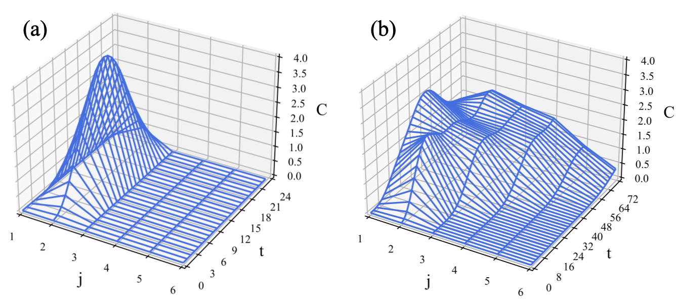
Figure 1: Commutator $C_{1j}(t)$ versus qubit position $j$ and time $t$. (a) Integrable regime, where no spreading occurs. The OTOC is calculated at times $t\in\{0,\tau,2\tau,\cdots,24\tau\}$, with resolution $\tau\!=\!0.06$, and time is plotted in units of $\tau$. (b) Chaotic regime, calculated with $\tau\!=\!0.03$, showing ballistic operator spreading. Parameters for both regimes are given in Table 1.

In this work we use quantum simulation techniques to study spreading of the Pauli operator $X(t)\!=\!e^{iHt}Xe^{-iHt}$ in the Ising chain

$$H = H^{0}+B_{x}\sum_{i=1}^{n}X_{i},$$ (3)

$$H^{0} = J\sum_{i=1}^{n-1}Z_{i}Z_{i+1}+B_{z}\sum_{i=1}^{n}Z_{i},$$ (4)

with $n$ spins. The model is separated into a classical Ising chain $H^{0}$ plus a noncommuting transverse field. The model (3) permits efficient Hamiltonian simulation via Trotterization. $H^{0}$ is also exactly solvable, a property used below. We measure and plot the commutator

$$C_{ij}(t)={\rm tr}(\rho\big{|}[X_{i}(t),X_{j}(0)]\big{|}^{2})=2-2\,{\rm Re}\,F_{ij}(t),$$ (5)

in the state $\rho=|0000\rangle\langle 0000|$, with $X(t)$ initially localized at $i\!=\!1$. In particular, we study $C_{1j}$ as a function of qubit position $j\in\{1,2,\dots,N\}$ and time $t$. The quantum simulations are implemented on the IBM Q processor ibmq_sydney using qubits $\{Q_{1},Q_{2},Q_{3},Q_{5}\}$ SI. The measured OTOC is

$$F_{1j}(t)=\langle 0000|U^{\dagger}X_{1}UX_{j}U^{\dagger}X_{1}UX_{j}|0000\rangle,$$ (6)

where $U$ is a 4-qubit circuit simulating $e^{-iHt}$. The commutator (5) was chosen because it exhibits a particularly smooth, easily visualized dynamics, using an easy-to-prepare state. Operator spreading diagnosed by alternative commutators are compared in SI.

In the experiments we always use one of the two parameter sets given in Table 1, both of which simulate ferromagnetic spin chains. One set corresponds to an integrable regime of the dynamics; the other generates quantum chaos, which causes unitary OTOC decay. The models are chosen to display smooth charge spreading dynamics on the timescales of interest. The measurements in the integrable regime are relevant for recent theoretical work investigating the role of integrability on scrambling lin2018out; fortes2019gauging, as well as serving as a scrambling-free experimental control. The commutator (5) is a real number $0\leq C_{1j}(t)\leq 4$, and can be represented by a surface in spacetime $j\!\times\!t$. Figure 1 shows two such surfaces, obtained by classical simulation, for $n\!=\!6$. These simulations assume perfect Hamiltonian simulation $U=e^{-iHt}$ with no Trotter error. Operator localization in Fig. 1a and spreading in Fig. 1b are evident. These high-resolution simulations allow one to investigate operator spreading dynamics in great detail.

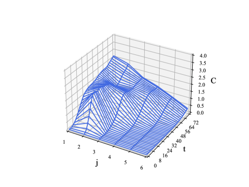
Figure 2: Chaotic $C_{1j}(t)$ commutator of Fig. 1b recalculated with the fixed-node OTOC.

Table 1: Ising model parameters.

	$J$	$B_{x}$	$B_{z}$
Integrable regime	-1	0	1
Chaotic regime	-1	0.7	1.5

Fixed-node OTOC. A standard approach to measuring an OTOC on $n$ qubits is to add a qubit that can control the $W$ and $V$ gates swingle2016measuring; zhu2016measurement. Here we introduce an alternative approach, which is approximate but allows one to reach larger problem sizes. Writing the OTOC in polar form as $F_{ij}=e^{i\arg F_{ij}}\,|F_{ij}|$, we note that the phase becomes irrelevant in the scrambling regime, because $|F_{ij}|\approx 0$ there. $|F_{ij}|$ can be measured directly with no qubit overhead swingle2016measuring, at least on simple states. Therefore we introduce an approximation for $\arg F_{ij}$ that is exact in the integrable regime, namely $\arg F_{ij}^{0}$, where $F_{ij}^{0}$ is the OTOC calculated with the classical Hamiltonian $H^{0}.$ For the Ising model (3),

$$F^{0}_{1j}(t)=\begin{cases}e^{4i(J+B_{z})t}&{\rm if}\ j=1,\\ e^{4iJt}&{\rm if}\ j=2,\\ 1&{\rm if}\ j>2.\\ \end{cases}$$ (7)

This results in a fixed-node variant of the OTOC,

$$F_{ij}=e^{i\arg F_{ij}^{0}}\,|F_{ij}|.$$ (8)

One can think of the fixed-node OTOC as an approximation to (2), or as an independent quantity that also diagnoses scrambling.

Using the fixed-node OTOC, the commutator takes the form

$$C_{ij}=2-2|F_{ij}|\cos(\arg F_{ij}^{0}).$$ (9)

The chaotic surface of Fig. 1b, recalculated with the fixed-node OTOC, is shown in Fig. 2.

By construction, the fixed-node OTOC is close to the exact OTOC in the late time regime, where $F_{ij}\approx 0\ (C_{ij}\approx 2)$. However, it also satisfies an important causality constraint that extends its accuracy to the regime of $F_{ij}\approx 1\ (C_{ij}\approx 0)$ as well, namely, the early scrambling regime. Causality requires that the exact OTOC satisfies $F_{ij}=1$ outside the lightcone, i.e. when $|{\bf r}_{i}-{\bf r}_{j}|>vt$, with ${\bf r}_{i,j}$ the local operator positions and $v$ the butterfly velocity. Therefore ${\rm arg}(F_{ij})\!=\!0$ there. Because $F_{ij}^{0}$ also satisfies this constraint, $C_{ij}$ computed from the fixed-node OTOC is also accurate outside the lightcone, as is evident in Fig. 2. Thus, while there are small differences in the peak structure in $C_{1j}(t)$, mainly at $j\!=\!1$, the overall spreading dynamics is accurately captured. The fixed-node commutator in the integrable regime is identical to the surface of Fig. 1a.

Figure 3: (Color online) Weaved time evolution. (a) Standard Trotter method, where a step $U(\tau)$ is repeatedly applied. (b) Weaving implements a fine-grained time evolution, with time resolution $\tau$, without incurring the gate errors of (a). Here the red column represents the sequence $U(k\tau)\cdots U(k\tau)$, orange represents $U(k\tau)\cdots U(k\tau)U(\tau)$, yellow represents $U(k\tau)\cdots U(k\tau)U(2\tau)$ and purple represents $U(k\tau)\cdots U(k\tau)\,U((k\!-\!1)\tau).$

Trotter weave. To measure $C_{ij}(t)$ with the high time resolution used in Fig. 1, one might construct a Trotter approximation $U(\tau)\approx e^{-iH\tau}$ for evolution by a short time $\tau$. Then, to simulate later times $t\!=\!\ell\tau$, the operator $U(\tau)$ is applied $\ell$ times:

$$e^{-iH\ell\tau}\approx U(\tau)^{\ell}\!.$$ (10)

The value of $\tau$ determines the time resolution. However, the circuit depth resulting from this standard Trotterization, based on the repeated application of a single step $U(\tau)$, is $t/\tau$. Thus, the performance of (10) quickly degrades with $t$ due to gate errors and decoherence, limiting the simulation to short times. We address this by an extension of Trotter simulation based on a collection of elementary evolution operators.

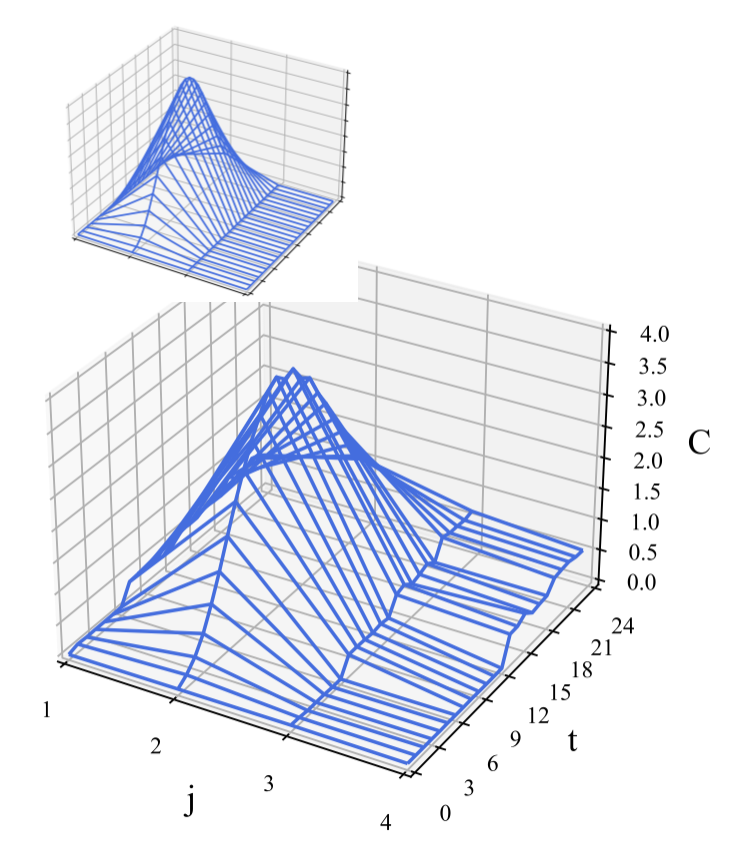
Figure 4: (Color online) Measured operator spreading surface in the integral regime, using the fixed-node OTOC. The main figure uses a 6-weave with $\tau=0.06$, and includes both CNOT and measurement error mitigation. $C_{1j}$ is defined in (5), with $j\in\{1,2,3,4\}$ the coordinate of the probe qubit. The OTOC is measured at times $t\in\{0,\tau,2\tau,3\tau,\cdots,24\tau\}$, and time is plotted in units of $\tau$. The inset shows the classically computed noise-free surface.

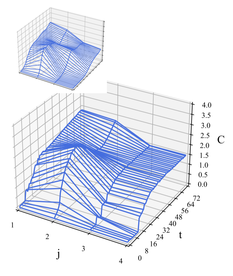
Figure 5: (Color online) Operator spreading in the chaotic regime using the fixed-node OTOC. We use a 6-weave with $\tau=0.03$, and also include error mitigation. The OTOC is measured at times $t\in\{0,\tau,2\tau,\cdots,72\tau\}$. The inset shows the noise-free surface.

A $k$-weave is a set of $k$ unitaries

$$\bigg{\{}U(\tau),U(2\tau),\cdots,U(k\tau)\bigg{\}},$$ (11)

where $\tau$ is a fixed short evolution time and each $U(dt)$ is a Trotterized evolution operator, propagating a state for a short time $dt$. The integer $k\in\{1,2,3,\cdots\}$ is called the weave modulus. The unitaries in (11) have different roles: $U(k\tau)$ is the cell operator and the remaining $k-1$ unitaries are called shift operators. Repeated applications of the cell propagates a state from $t=0$ to a time $t=(\ell-\ell\,{\rm mod}\,k)\!\times\!\tau$, but with coarse time resolution $k\tau$. The coarse evolution is then followed (or preceeded) by a single shift operator propagating for a short interval with fine-grained time precision $\tau$. Instead of (10), weaving implements a time evolution according to

$$e^{-iH\ell\tau}\approx U(k\tau)^{\frac{\ell-\ell{\rm mod}k}{k}}U(\ell\,{\rm mod}\,k\times\tau),$$ (12)

where the cell operator is applied $(\ell-\ell\,{\rm mod}\,k)/k$ times after a single shift operator. This is illustrated in Fig. 3. When $\ell\gg k$, this leads to a $k$-fold reduction in circuit depth, and to higher circuit fidelity, at the expense of increased of Trotter error. Weaving can be applied to Hamiltonian simulation techniques beyond Trotterization as well.

For our first set of measurements we use the weave operators $\{U(\ell\tau)\}_{\ell=1}^{k}$, where

$$U(\ell\tau) = \prod_{i=1}^{n}\!R_{\rm x}(B_{x}\ell\tau)_{i}\times\prod_{i=1}^{n-1}\!R_{\rm zz}(2J\ell\tau)_{i,i+1}\$$ (13)

$$\times \prod_{i=1}^{n}\!P_{\rm z}(2B_{z}\ell\tau)_{i}\times\prod_{i=1}^{n}\!R_{\rm x}(B_{x}\ell\tau)_{i},$$

resulting from a Trotterization of the model (3). Here $R_{x}(\theta)_{i}\!=\!e^{-i\theta X_{i}/2}$ is a rotation on qubit $i$,

$$R_{zz}(\theta)_{ij}=e^{-i\frac{\theta}{2}Z_{i}\otimes Z_{j}}={\rm CNOT}_{ij}\ P_{z}(\theta)_{i}\ {\rm CNOT}_{ij}\ \ \ \ \$$ (14)

is a $ZZ$ rotation, $P_{z}(\varphi)\!=\!{\rm diag}(1,e^{i\varphi})$ is a phase gate, and ${\rm CNOT}_{ij}$ is an $X$ on qubit $j$ controlled by $i$. For general angles $\theta$, $R_{zz}(\theta)_{ij}$ requires two CNOTs per graph edge, or $2(n-1)$ CNOTs per Trotter step on a chain of length $n$. The quantum simulation results reported here use (up to) two weave operators per Hamiltonian simulation, requiring $4(n-1)$ CNOTs per evolution. This leads to a total of $16(n-1)$ CNOTs per OTOC simulation (48 CNOTs for $n=4$).

Results. All of the quantum simulation results in this study were obtained with the IBM Q processor ibmq_sydney on the 4-qubit chain $\{Q_{1},Q_{2},Q_{3},Q_{5}\}$ SI. Quantum simulations using Trotter weave modulus $k=6$ are shown in Figs. 4 and 5. Figure 4 shows the measured spreading surface $C_{1j}(t)$ in an integral regime of the spin chain. Figure 5 is the same, but calculated in a chaotic regime of the model. The parameter values used are shown in Table 1. The data in both regimes are corrected for measurement errors using transition matrix error mitigation maciejewski2020mitigation; nachman2020unfolding; hamilton2020scalable; bravyi2021mitigating; geller2021toward, and for incoherent CNOT errors using zero-noise extrapolation temme2017error; dumitrescu2018cloud. The raw data from this study is provided in SI.

The values of $\tau$ (time resolution) and $k$ (weave modulus) are chosen to balance gate errors and Trotter errors over the relevant time scales of the simulation. In particular, $\tau$ has to be small enough to resolve the oscillations in the peaks of the spreading surfaces (see Figs. 1 and 2). However, $\tau$ also has to be large enough to enable simulations that probe the long-time spreading dynamics. A large value of $k$ is desirable because it enables longer simulations, as fewer applications of the cell circuit are required. But a large value of $k$ also leads to larger Trotter errors in the weave operators.

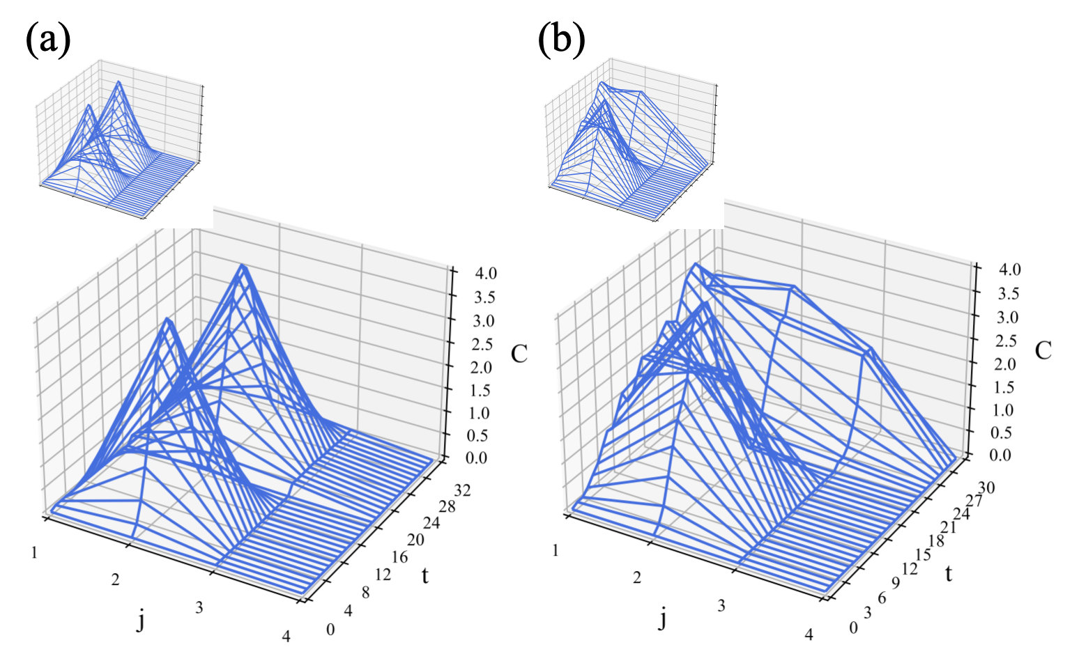
Figure 6: (Color online) Measured operator spreading surfaces using the fixed-node OTOC and magic cell operator. (a) 16-weave in the integrable regime with $\tau=0.098$ and up to 32 steps. (b) 20-weave in the chaotic regime with $\tau=0.079$ and up to 30 steps. Insets show the noise-free surfaces.

Magic cell. In many weaving applications, the largest Trotter error will come from the cell $U(k\tau)$, because its evolution time $k\tau$ is largest. However, some simulations admit simplified Trotter steps $U(dt)$ for certain “magic” values of $dt$. In the Ising chain, for example, this occurs when $2J\,dt=\pm\frac{\pi}{2},$ because for these angles we can use the decomposition

$$R_{zz}({\textstyle\frac{\pi}{2}})_{ij}=e^{-i\frac{\pi}{4}Z_{i}\otimes Z_{j}}=e^{-i\frac{\pi}{4}}S_{i}S_{j}{\rm CZ}_{ij},\ \ \$$ (15)

or its Hermitian conjugate, instead of (14). Here $S\!=\!{\rm diag}(1,e^{i\frac{\pi}{2}})$ and CZ is a controlled-$Z$ gate that can be implemented using a single CNOT and two Hadamard gates. This leads to a two-fold reduction in the number of CNOTs required. We demonstrate this variation, where the weave is built around a magic cell operator with evolution time $dt_{\rm magic}\!=k\tau=\pi/4|J|$. Because $dt_{\rm magic}$ is now fixed to a special value, the use of a magic cell imposes a constraint $dt_{\rm magic}\!=\!k\tau$ on $k$ and $\tau$; they are no longer independent. Operator spreading measurements using a 16-weave with magic cell in the integrable regime, and a 20-weave with magic cell in the chaotic regime, are shown in Fig. 6. The parameter values used are shown in Table 1. The data in both regimes are error mitigated. The benefits of using a magic cell here are modest, because we only apply it once. However, the use of a magic cell has the potential to significantly extend the range of Trotterized quantum simulation as gate errors improve and larger circuits become possible.

Conclusions. Recent experiments have established that scrambling can be simulated with current gate-based quantum computers landsman2019verified; blok2021quantum; chen2020detecting; niknam2020sensitivity; mi2021information; braumuller2021probing; chen2021observation; joshi2020quantum; zhu2021observation, making it possible to investigate interesting unsolved problems at the intersection of quantum information and physics. In this work we introduce and demonstrate techniques to enable high-resolution operator spreading measurements with cloud-based quantum computers. Trotter weaving provides the high time resolution, and the fixed-node OTOC enables larger problem sizes. Both approaches are practical for online users and have applications elsewhere in quantum information science. We observe clear signatures of operator spreading in a chaotic regime of a 4-qubit Ising model, as well as operator localization in an integrable regime. These techniques help make it possible to study information dynamics in strongly correlated and highly entangled quantum systems.

Acknowledgments. We thank Andreas Albrecht for useful discussions. PJC and AS acknowledge initial support and MRG acknowledges support from LANL’s Laboratory Directed Research and Development (LDRD) program under project number 20190065DR. AA and ZH acknowledge, and PJC and AS acknowledge (subsequent to the above acknowledged funding) that this work was supported by the U.S. Department of Energy, Office of Science, Office of High Energy Physics QuantISED program under Contract No. KA2401032. ZH acknowledges support from the LANL LDRD-funded Mark Kac Postdoctoral Fellowship. BY acknowledges support of the U.S. Department of Energy, Office of Science, Basic Energy Sciences, Materials Sciences and Engineering Division, Condensed Matter Theory Program, and partial support from the Center for Nonlinear Studies.

Supplementary Information for
“Quantum Simulation of Operator Spreading in the Chaotic Ising Model”

This document provides additional details about the experimental results. Section 1 describes the online superconducting qubits used, and gives calibration results (gate errors, coherence times, and single-qubit measurement errors) provided by the backend. Section 2 presents raw data. In Sec. 3 we discuss the error mitigation techniques used and their effect on the data. In Sec. 4 we calculate the OTOC for the classical Ising model $H^{0}$. Alternative OTOCs are discussed in Sec. 5.

1 Qubits

In this section we discuss the online superconducting qubits used in this work. Data was taken on the IBM Q processor ibmq_sydney using the BQP software package developed by the authors. We measure the OTOC on qubits $\{Q_{1},Q_{2},Q_{3},Q_{5}\}$ shown in Fig. S1. Calibration data supplied by the backend is summarized in Table 1. Here $T_{1,2}$ are the standard Markovian decoherence times, and

$$\epsilon=\frac{T(0|1)+T(1|0)}{2}$$ (S1)

is the single-qubit state-preparation and measurement (SPAM) error, averaged over initial classical states. $T(0|1)$ is the probability of measuring a $|0\rangle$ state after preparing $|1\rangle$; $T(1|0)$ is the reverse. The $U_{2}$ error column gives the single-qubit gate error measured by randomized benchmarking. The reported CNOT errors are also measured by randomized benchmarking.

Table 1: Calibration data provided by IBM Q for the ibmq_sydney chip during the period of data acquisition.

Qubit $T_{1}\ (\mu s)$ $T_{2}\ (\mu s)$ SPAM error $\epsilon$ $U_{2}$ error $Q_{1}$ 99.7 37.3 0.043 2.83e-4 $Q_{2}$ 107.9 65.5 0.015 1.80e-4 $Q_{3}$ 78.7 51.7 0.017 3.15e-4 $Q_{5}$ 147.4 61.1 0.017 1.64e-4

CNOT gates CNOT error ${\rm CNOT}_{1,2}$ ${\rm CNOT}_{2,1}$ 7.67e-3 ${\rm CNOT}_{2,3}$ ${\rm CNOT}_{3,2}$ 7.00e-3 ${\rm CNOT}_{3,5}$ ${\rm CNOT}_{5,3}$ 7.68e-3

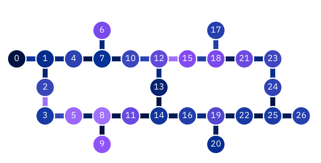
Figure S1: Layout of IBM Q device ibmq_sydney. In this work we use qubits $Q_{1}$, $Q_{2}$, $Q_{3}$ and $Q_{5}$.

2 Raw operator spreading data

The raw operator spreading surfaces are shown in Figs. S2 and S3. The differences between the raw and error-mitigated data are shown in Sec. 3.

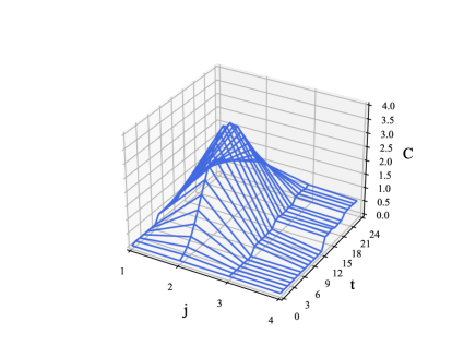
Figure S2: Raw spreading data in the integral regime, with the same settings as in Fig. 4.

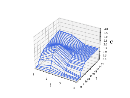
Figure S3: Raw spreading data in the chaotic regime, with the same settings as in Fig. 5.

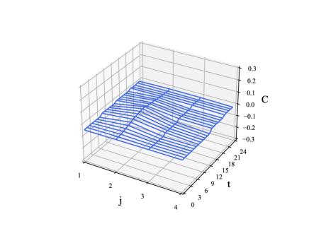
Figure S4: Difference $C_{\rm TMEM}\!-\!C_{\rm raw}$ between measurement-corrected and raw surfaces in the integrable regime.

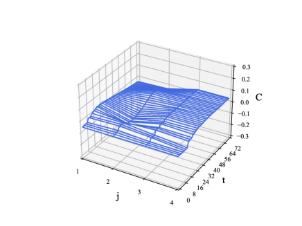
Figure S5: Difference $C_{\rm TMEM}\!-\!C_{\rm raw}$ between measurement-corrected and raw surfaces in the chaotic regime.

3 Error mitigation

In this work we correct all data for measurement errors using transition matrix error mitigation (TMEM)maciejewski2020mitigation; nachman2020unfolding; hamilton2020scalable; bravyi2021mitigating; geller2021toward, and for incoherent CNOT errors using zero-noise extrapolation temme2017error; dumitrescu2018cloud. In TMEM, the matrix $T$ of transition probabilities between all prepared and observed classical states $x\in\{0,1\}^{n}$ is initially measured. Then noisy data is corrected by minimizing $\|T\,p_{\rm corr}-p_{\rm noisy}\|_{2}^{2}$ subject to constraints $0\leq p_{\rm corr}(x)\leq 1$ and $\|p_{\rm corr}\|_{1}=1$. Here $\|\cdot\|_{2}$ is the Euclidean norm and $\|\cdot\|_{1}$ is the $\ell_{1}$-norm. The effect of TMEM on the operator spreading data is shown in Figs. S4 and S5.

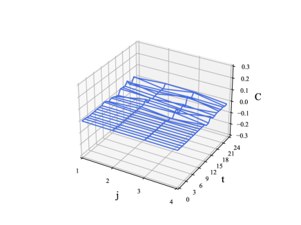
Figure S6: Difference $C_{\rm CNOT}\!-\!C_{\rm raw}$ between CNOT-corrected and raw surfaces in the integrable regime.

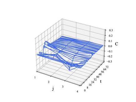
Figure S7: Difference $C_{\rm CNOT}\!-\!C_{\rm raw}$ between CNOT-corrected and raw surfaces in the chaotic regime.

The CNOT error mitigation involves measuring each circuit together with a variant, obtained by replacing each CNOT in the original circuit by a logically equivalent CNOT³. Let ${\rm Pr}(x|m)$ be the probability of observing classical state $x$ after implementing a circuit with each original CNOT replaced by $m$ consecutive CNOTs. Then let $\{{\rm Pr}(x|1)\}_{x}$ be a measured probability distribution for the original circuit, and $\{{\rm Pr}(x|3)\}_{x}$ be that for the CNOT³ variant. Assuming that the total incoherent CNOT error in the circuit occurs in proportion to the number of CNOTS implemented, one can use the two data points ${\rm Pr}(x|1)$ and ${\rm Pr}(x|3)$ to define a line with intercept

$${\rm Pr}(x|0):=\frac{3\,{\rm Pr}(x|1)-{\rm Pr}(x|3)}{2},$$ (S2)

which defines a candidate correction. Here $m=0$ means no incoherent CNOT error. If $0\leq{\rm Pr}(x|0)\leq 1$ for all $x$, then we accept it as the corrected probability distribution:

$${\rm Pr}(x)_{\rm corr}={\rm Pr}(x|0).$$ (S3)

Otherwise we find the physical ${\rm Pr}(x)_{\rm corr}$ closest to ${\rm Pr}(x|0)$ in Frobenius distance. The effect of CNOT noise extrapolation on the operator spreading data is shown in Figs. S6 and S7.

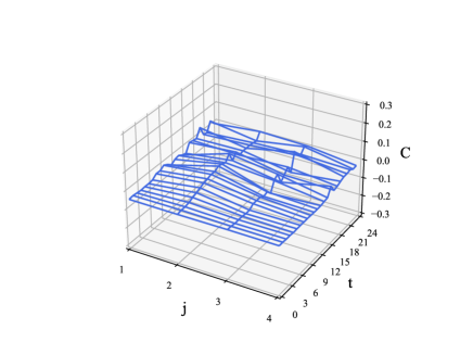
Figure S8: Difference $C_{\rm corr}\!-\!C_{\rm raw}$ between fully corrected and raw surfaces in the integrable regime.

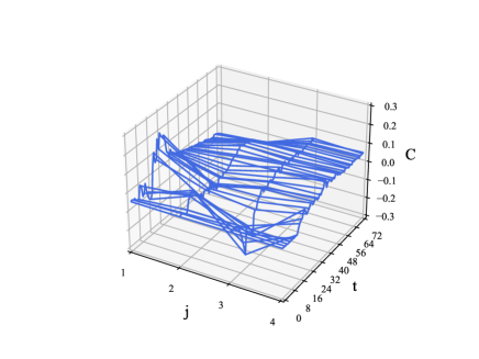
Figure S9: Difference $C_{\rm corr}\!-\!C_{\rm raw}$ between fully corrected and raw surfaces in the chaotic regime.

The net effect of TMEM and CNOT noise extrapolation on the operator spreading data is shown in Figs. S8 and S9. When both error mitigations are applied to the raw operator spreading data, we obtain the surfaces in Figs. 4 and 5.

4 Classical OTOC

In the fixed-node approach, the absolute value of the OTOC is measured on the quantum processor but its phase is efficiently calculated from $F_{ij}^{0}$, the OTOC (6) calculated with the classical Hamiltonian $H^{0}$ of (4). To calculate this phase, we need the energy of the $n$-qubit state $|0\cdots 0\rangle$, which is

$$E_{0}=(n-1)J+nB_{z}.$$ (S4)

Next we assume that $n\geq 3$. The energy of the single-excitation state $X_{j}|0\cdots 0\rangle=|0\cdots 1_{j}\cdots 0\rangle$ is

$$E_{0\cdots 1_{j}\cdots 0}=\begin{cases}E_{0}-2J-2B_{z}&{\rm if}\ j\in\{1,n\},\\ E_{0}-4J-2B_{z}&{\rm else}.\\ \end{cases}$$ (S5)

We will also need the energy of the double-excitation state $|10\cdots 1_{j}\cdots 0\rangle$, with $j\geq 2$, which is

$$E_{10\cdots 1_{j}\cdots 0}=\begin{cases}E_{0}-2J-4B_{z}&{\rm if}\ j=2,\\ E_{0}-4J-4B_{z}&{\rm if}\ j=n,\\ E_{0}-6J-4B_{z}&{\rm else}.\\ \end{cases}$$ (S6)

To calculate the OTOC we first write it as

$$F^{0}_{1j}(t)=\sum_{x}\langle 0\cdots 0|X_{1}(t)X_{j}|x\rangle\langle x|X_{1}(t)X_{j}|0\cdots 0\rangle,$$ (S7)

where $|x\rangle$ is a classical state with $x\in\{0,1\}^{n}$. If $j=1$ we have

$$F^{0}_{11}(t) = \langle 0\cdots 0|X_{1}(t)|10\cdots 0\rangle^{2}$$ (S8)

$$= \langle 0\cdots 0|e^{iE_{0}t}X_{1}e^{-i(E_{0}-2J-2B_{z})t}|10\cdots 0\rangle^{2}$$

$$= e^{4i(J+B_{z})t},$$

where we have used (S5).

If $j>1$, we have

$$F^{0}_{1j}(t) = \sum_{x}\langle 0\cdots 0|X_{1}(t)X_{j}|x\rangle\langle x|X_{1}(t)X_{j}|0\cdots 0\rangle$$ (S9)

$$= \langle 0\cdots 0|X_{1}(t)|10\cdots 0\rangle\langle 10\cdots 1_{j}\cdots 0|X_{1}(t)|0\cdots 1_{j}\cdots 0\rangle$$ (S10)

$$= \langle 0\cdots 0|e^{iE_{0}t}X_{1}e^{-iHt}|10\cdots 0\rangle\langle 10\cdots 1_{j}\cdots 0|e^{iHt}X_{1}e^{-iHt}|0\cdots 1_{j}\cdots 0\rangle$$ (S11)

$$= e^{2i(J+B_{z})t}\langle 10\cdots 1_{j}\cdots 0|e^{iHt}X_{1}e^{-iHt}|00\cdots 1_{j}\cdots 0\rangle,$$ (S12)

and there are three cases to consider: When $j=2$, (S12) becomes

$$F^{0}_{12}(t) = e^{2i(J+B_{z})t}\langle 110\cdots 0|e^{iHt}X_{1}e^{-iHt}|01\cdots 0\rangle$$ (S13)

$$= e^{2i(J+B_{z})t}\langle 110\cdots 0|e^{i(E_{0}-2J-4B_{z})t}X_{1}e^{-i(E_{0}-4J-2B_{z})t}|01\cdots 0\rangle$$ (S14)

$$= e^{2i(J+B_{z})t}e^{2i(J-B_{z})t}$$ (S15)

$$= e^{4iJt},$$ (S16)

where we have used (S6). When $2<j<n,$ (S12) becomes

$$F^{0}_{1j}(t) = e^{2i(J+B_{z})t}\langle 10\cdots 1_{j}\cdots 0|e^{iHt}X_{1}e^{-iHt}|0\cdots 1_{j}\cdots 0\rangle$$ (S17)

$$= e^{2i(J+B_{z})t}\langle 10\cdots 1_{j}\cdots 0|e^{i(E_{0}-6J-4B_{z})t}X_{1}e^{-i(E_{0}-4J-2B_{z})t}|0\cdots 1_{j}\cdots 0\rangle$$ (S18)

$$= e^{2i(J+B_{z})t}e^{-2i(J+B_{z})t}$$ (S19)

$$= 1.$$ (S20)

And when $j=n$, (S12) becomes

$$F^{0}_{1n}(t) = e^{2i(J+B_{z})t}\langle 10\cdots 01|e^{iHt}X_{1}e^{-iHt}|0\cdots 01\rangle$$ (S21)

$$= e^{2i(J+B_{z})t}\langle 10\cdots 01|e^{i(E_{0}-4J-4B_{z})t}X_{1}e^{-i(E_{0}-2J-2B_{z})t}|0\cdots 01\rangle$$ (S22)

$$= e^{2i(J+B_{z})t}e^{-2i(J+B_{z})t}$$ (S23)

$$= 1.$$ (S24)

Combining these results leads to the expression (7).

5 Other OTOCs

The operator spreading measurements in this work are based on the commutator

$${\rm tr}(\rho\big{|}[X_{i}(t),X_{j}(0)]\big{|}^{2})\ \ {\rm with}\ \ \rho=|0000\rangle\langle 0000|.\ \ \$$ (S25)

It is interesting to compare (S25) with alternative definitions. A common alternative is the infinite-temperature version

$${\rm tr}(\rho\big{|}[X_{i}(t),X_{j}(0)]\big{|}^{2})\ \ {\rm with}\ \ \rho=\frac{I}{d},\ \$$ (S26)

where $I$ is the $d\times d$ identity with $d=2^{n}$. The operator spreading surfaces of Fig. 1, reevaluated with (S26), are shown in Fig. S10. These surfaces are ideal results obtained classically. Overall the spreading is similar to Fig. 1, but there are detailed differences.

It is also interesting to consider a pure state different than $|0\rangle^{\otimes n}$, such as $|+\rangle^{\otimes n}$. Figure S11 is based on the commutator

$${\rm tr}(\rho\big{|}[X_{i}(t),X_{j}(0)]\big{|}^{2})\ \ {\rm with}\ \ \rho=\frac{J}{d},\ \$$ (S27)

where $J$ is the $d\times d$ matrix of ones.

Finally, we consider the commutator

$${\rm tr}(\rho\big{|}[X_{i}(t),Y_{j}(0)]\big{|}^{2})\ \ {\rm with}\ \ \rho=|0000\rangle\langle 0000|,\ \ \$$ (S28)

which has a peak structure different from (S25) because $[X_{i}(t),Y_{j}(0)]\neq 0$ at time 0. The operator spreading surfaces of Fig. 1, reevaluated with (S28), are shown in Fig. S12.

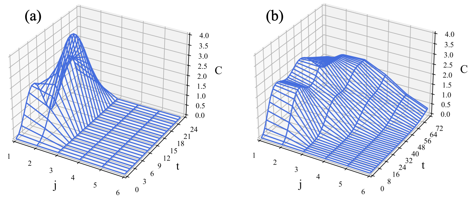
Figure S10: Infinite-temperature commutator versus qubit position $j$ and time $t$. (a) Integrable regime. The OTOC is calculated at times $t\in\{0,\tau,2\tau,\cdots,24\tau\}$, with resolution $\tau\!=\!0.06$, and time is plotted in units of $\tau$. (b) Chaotic regime, calculated with $\tau\!=\!0.03$. Parameters for both regimes are given in Table 1. These results were obtained by classical simulation.

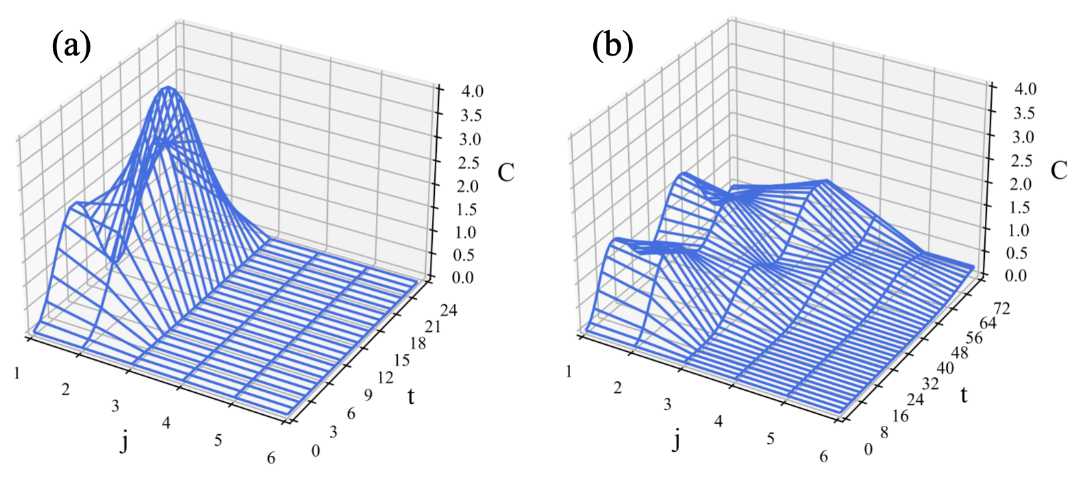
Figure S11: Operator spreading in the $|+\rangle^{\otimes n}$ state, with other parameters the same as in Fig. S10.

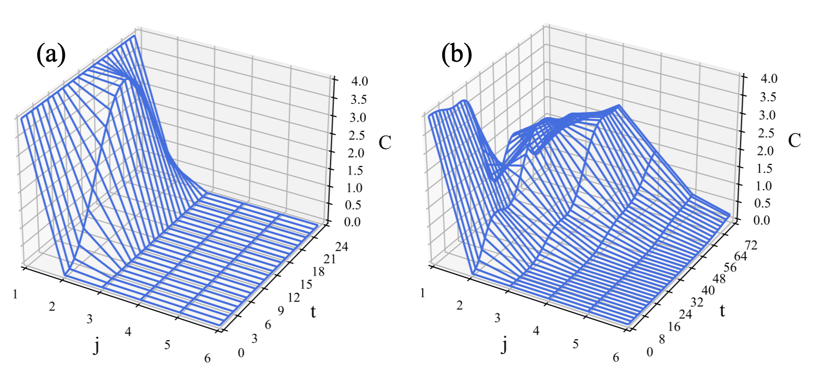
Figure S12: Spreading of $X_{1}$ probed by $Y_{j}$, with other parameters the same as in Fig. S10..