Fine and hyperfine splitting of the low-lying states of ${}^{9}$Be

Abstract

We perform accurate calculations of energy levels as well as fine and hyperfine splittings of the lowest ${}^{1,3}\!P_{J}$, ${}^{3}\!S_{1}$, ${}^{3}\!P^{e}_{J}$, and ${}^{1,3}\!D_{J}$ excited states of the ${}^{9}$Be atom using explicitly correlated Gaussian functions and report on the breakdown of the standard hyperfine structure theory. Because of the strong hyperfine mixing, which prevents the use of common hyperfine constants, we formulate a description of the fine and hyperfine structure that is valid for an arbitrary coupling strength and may have wide applications in many other atomic systems.

I Introduction

The main drawback of atomic structure methods based on the nonrelativistic wave function represented as a linear combination of determinants of spin-orbitals (Hartree-Fock, configuration interaction, multi-configurational self-consistent field, etc.) is the difficulty in providing results with reliably estimated uncertainties. While the accuracy of nonrelativistic energy can be assessed by increasing the space of electronic configurations, the irregular convergence of matrix elements, especially involving singular operators, such as those for relativistic or quantum electrodynamics (QED) corrections, often does not allow for presenting any uncertainties. Therefore, this deficiency limits the use of these methods in the high-accuracy-demanding applications, e.g. testing quantum electrodynamics [Nortershauser:15, Pachucki:17, Alighanbari:20], determination of the nuclear charge radii [Sanchez:06, Sturm:14, Manovitz:19, Maass:19], the nuclear electromagnetic moments [Stone:15, Puchalski:21], or physical constants [CODATA:18], and searching for new physics [Safronova:18].

On the other hand, an alternative approach based on the Dirac-Coulomb Hamiltonian, with the wave function represented as a determinant of four-component spin-orbitals of positive energy, can reach reasonably convergence on relativistic energies and matrix elements [Derevianko0]. But so far there is no formulation of QED theory on the top of Dirac-Coulomb Hamiltonian with projection on positive one-electron energies. Therefore numerical convergence does not say much about uncertainties due to omitted QED effects, including those related to negative energy orbitals. Another problems arise when the hyperfine effects are not negligible compared to the fine structure splitting. In the previous works on this topic (e.g. [Derevianko1, Derevianko2]), it has been demonstrated the hyperfine mixing of fine structure levels can be satisfactorily accounted for by the second-order perturbation theory. However, when the hyperfine splitting is of the same order or even larger than the fine structure splitting, the perturbative approach fails, and one can no longer use the standard $A_{J}$ and $B_{J}$ hyperfine parameters.

It is desirable therefore to develop tools which provide high and controlled accuracy, like those based on nonrelativistic QED (NRQED) theory and representation of the nonrelativistic wave function in terms of explicitly correlated basis functions, e.g. exponential, Hylleraas, or Gaussian (ECG) ones. The controlled accuracy is achieved by means of a full variational optimization of the wave function and by transformation of singular operators to an equivalent but more regular form. The price paid for using the explicitly correlated functions is the rapid increase in the complexity of calculations with each additional electron; therefore, application of these functions has so far been limited to few-electron systems only.

Before passing to the main topic, which is the 4-electron beryllium (Be) atom, let us briefly describe recent advances in the calculation of 1-, 2-, and 3-electron atomic systems. Hydrogenic systems are the only ones in which theoretical predictions including QED effects are sufficiently accurate to determine the nuclear (proton, deuteron) charge radius from the measured transition frequencies [CODATA:18]. Being apparently simple, hydrogenic systems are a cornerstone for the implementation of QED in bound states, which relies on the expansion of binding energy in powers of the fine structure constant $\alpha\sim 1/137$. Similarly, for two- and more-electron systems, one also performs expansion in $\alpha$, as long as the nuclear charge $Z$ is not too large. This allows description of an atomic system in terms of the successively smaller effects, i.e. nonrelativistic energy $\alpha^{2}$, relativistic correction $\alpha^{4}$, leading QED of order $\alpha^{5}$, and so on. For the helium atom all these expansion terms are calculated up to the order $\alpha^{6}$ [Yerokhin:10], with some states up to the order $\alpha^{7}$ [Patkos:21]. Such high order calculations are feasible with explicitly correlated exponential basis functions, for which analytic integrals are known. Atomic systems with three electrons present greater difficulty for the accurate calculation of their energy levels despite obtaining very precise wave functions with explicitly correlated Hylleraas or ECG functions. Nevertheless, several highly accurate results have been obtained for Li and Be${}^{+}$, including isotope shifts for the charge radii determination [Sanchez:06, Northershauser:09, Krieger:12], and fine [Puchalski:14] and hyperfine [Puchalski:13b] splitting. The fine structure splitting of the lithium $2^{2}\!P_{J}$ state with the inclusion of $O(\alpha^{6})$ QED corrections [Puchalski:14, Wang:17] agrees well with even more accurate experimental values [Brown:13, Li:20], while current theoretical predictions for the ${}^{6/7}$Li ground state hyperfine splitting are limited by insufficient knowledge of the nuclear structure, and not by the atomic structure theory.

The experience gained from the above-mentioned systems can be exploited to a large extent in four-electron systems, but these ones are much more demanding in calculations. The attempts employing Hylleraas wave functions [Busse:98, King:11, Sims:11] are limited to nonrelativistic energy because of the lack of effective methods of evaluation of ”relativistic” four-electron integrals. Therefore, our choice is the use of the ECG method, which performs very well for both nonrelativistic and relativistic contributions [Komasa:95, Busse:98, Komasa:01a, Komasa:01b, Komasa:02a, Komasa:02b, Pachucki:04, PK06b, Stanke:07a, Stanke:07b, Stanke:09, Chen:09, Bunge:10, King:11, Sims:11, Sharkey:11, Chen:12, Bubin:12, Puchalski:13a, Puchalski:14a, Sharkey:14, Stanke:19, Kedziorski:20]. Nonetheless, we note that because Gaussian-type wave functions do not satisfy the Kato cusp condition, the complete calculation of the $\alpha^{6}$ correction is still unfeasible. This unsolved problem limits the current capabilities of the ECG method in the application to three- and more-electron systems. After all, the ECG functions are so far the best suited for the four-electron systems and such an application to the Be atom will be presented here.

In our previous works on Be we have obtained accurate energies for the ground $2s^{2}\,{}^{1}\!S_{0}$ and the excited $2s2p\,^{1}\!P_{1}$ states [Puchalski:13a], the difference of which at $42\,565.441(11)\,\mathrm{cm}^{-1}$, agrees well with the experimental value of $42\,565.450\,1(13)\,\mathrm{cm}^{-1}$ obtained by Cook et al. [Cook:18] and with later calculations [Hornyak:19]. Last year, two more transitions were measured to a high accuracy—the wavenumber of the $2s^{2}\,{}^{1}\!S_{0}-2s3d\,^{1}\!D_{2}$ line, equal to $64\,428.403\,21(55)\,\mathrm{cm}^{-1}$, and of the $2s2p\,^{1}\!P_{1}-2s3d\,^{1}\!D_{2}$ line, equal to $21\,862.952\,9(14)\,\mathrm{cm}^{-1}$, were reported by Cook et al. [Cook:20]. In this case, no theoretical results at an adequate level of accuracy have been calculated yet. Moreover, in the beryllium atom, of particular theoretical interest is the lowest $2s2p\,^{3}\!P$ excited state, because it is metastable. So far though, its energy has not been measured and calculated to such a high accuracy as for the $2s2p\,^{1}\!P$ state. An old but the most accurate experimental excitation energy from the ground to the $2s2p\,^{3}\!P_{1}$ level equal to $21\,978.92(1)~{}\mathrm{cm}^{-1}$ [Bozman:53] is in agreement with the less accurate recent theoretical value of $21\,978.2(11)~{}\mathrm{cm}^{-1}$ by Kedziorski et al. [Kedziorski:20]. Quite recently, the hyperfine splitting of the $2s2p\,^{3}\!P$ state has been accurately calculated and, with the help of the 50-years old measurements by Blachman [Blachman:67], has been employed to determine the most accurate value of the electric quadrupole moment of ${}^{9}$Be [Puchalski:21], but it is in disagreement with all previous determinations. Moreover, all the other Be energy levels lying below the ionization threshold of $75\,192.64\,\mathrm{cm}^{-1}$ have large uncertainties, being in the range $0.01-0.2\,\mathrm{cm}^{-1}$ [Kramida:20], and there are no corresponding accurate theoretical results to compare with.

The purpose of the present work is therefore to significantly advance the theoretical description of the lowest excited states with different internal symmetries. Namely, we focus on states with non-vanishing spin or orbital angular momentum and verify the previous literature results, which were obtained using either the ECG method or methods based on one-electron approximation. More precisely, we report on ECG calculations for the six lowest excited states of the ${}^{9}$Be atom: ${}^{1,3}\!P_{J}$, ${}^{3}\!S_{1}$, ${}^{3}\!P^{e}_{J}$, and ${}^{1,3}\!D_{J}$, including their fine and hyperfine splittings. Due to a significant hyperfine mixing, the standard hyperfine structure formulation in terms of $A_{J}$ and $B_{J}$ coefficients is not adequate in some cases. For this reason we have introduced a combined fine–hyperfine structure formalism that naturally accounts for an arbitrary mixing between fine and hyperfine levels. Moreover, in order to unify the description of atomic wave functions of different symmetries, we have introduced in this work a Cartesian angular momentum representation, which is tailored for use with many-electron explicitly correlated basis functions and which simplifies evaluation of matrix elements.

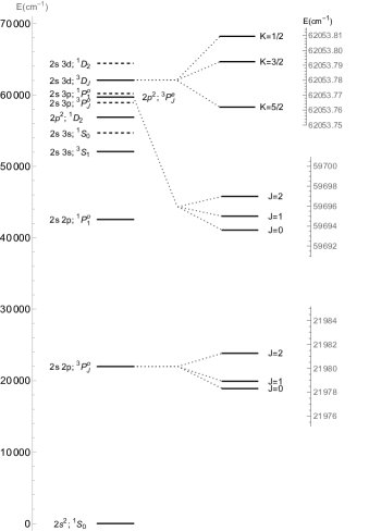
Figure 1: The lowest energy levels of theBe atom. The levels for which the energy is evaluated in this work are drawn in solid lines and the remaining ones in dashed line. The fine structure of the triplet states of our interest is also shown, $\vec{J}=\vec{L}+\vec{S},\vec{K}=\vec{I}+\vec{S}$.

II Theoretical framework

In the calculations of the energy levels of few-electron light atomic systems with a well controlled accuracy, we employ the expansion in the fine-structure constant $\alpha\approx 1/137$

$$E(\alpha)=E^{(2)}+E^{(4)}+E^{(5)}+E^{(6)}+\ldots,$$ (1)

where $E^{(n)}\sim m\,\alpha^{n}$ and some expansion terms may include finite powers of $\ln\alpha$. Uncalculated higher order terms will be estimated from the corresponding expansion terms in the hydrogenic limit, while the numerical accuracy is controlled by the varying the number of terms in the highly optimized explicitly correlated wave function.

II.1 Nonrelativistic energy

The leading term $E_{0}\equiv E^{(2)}$ is obtained from the non-relativistic Hamiltonian in the center-of-mass system ($\vec{p}_{N}=-\sum_{a}\vec{p}_{a}$) by solving the Schrödinger equation (in natural units)

$$H^{(2)}\Psi =E_{0}\Psi$$ (2)

$$H^{(2)} =\frac{\vec{p}^{2}_{N}}{2\,m_{N}}+\sum_{a}\frac{\vec{p}^{2}_{a}}{2\,m}-\sum_{a}\frac{Z\,\alpha}{r_{a}}+\sum_{a<b}\frac{\alpha}{r_{ab}}$$ (3)

where $Z$ is the nuclear charge, and $m$ and $m_{N}$ are the electron and nuclear masses, respectively. In this work, the effects of the finite nuclear mass (recoil) are included in $H^{(2)}$. This is in contrast to the perturbative approach based on additional expansion in the electron-nucleus mass ratio, which is particularly useful in the isotope shift calculations [Puchalski:14a]. Once the wave function $\Psi$ is determined, all the corrections to the nonrelativistic energy $E_{0}$ can be expressed in terms of expectation values $\langle\Psi|\ldots|\Psi\rangle\equiv\langle\ldots\rangle$ of known operators.

II.2 Leading order corrections

The leading relativistic $E^{(4)}$ correction is calculated as the mean value of the Breit-Pauli Hamiltonian [Bethe:77]. For convenience, we split this Hamiltonian, according to its inner composition, into three parts: the no-spin (ns), the fine-structure (fs), and the hyperfine-structure (hfs) part

$$H^{(4)}=H_{\rm ns}^{(4)}+H_{\rm fs}^{(4)}+H_{\rm hfs}^{(4)}\,.$$ (4)

The spin-independent part in its explicit form is

$$H^{(4)}_{\rm ns}= \ \sum_{a}\Big{[}-\frac{\vec{p}^{4}_{a}}{8\,m^{3}}+\frac{\pi\,Z\,\alpha}{2\,m^{2}}\,\delta^{3}(r_{a})$$ (5)

$$\qquad+\frac{Z\,\alpha}{2\,m\,m_{N}}\,p_{a}^{i}\,\biggl{(}\frac{\delta^{ij}}{r_{a}}+\frac{r^{i}_{a}\,r^{j}_{a}}{r^{3}_{a}}\biggr{)}\,p_{N}^{j}\Big{]}$$

$$+\sum_{a<b}\Bigg{[}\frac{\pi\,\alpha}{m^{2}}\,\delta^{3}(r_{ab})-\frac{\alpha}{2\,m^{2}}\,p_{a}^{i}\,\biggl{(}\frac{\delta^{ij}}{r_{ab}}+\frac{r^{i}_{ab}\,r^{j}_{ab}}{r^{3}_{ab}}\biggr{)}\,p_{b}^{j}\Bigg{]}.$$

The part related to the fine-structure effects, containing the vector $\vec{\sigma}_{a}$ of Pauli spin matrices of electron $a$, can be expressed as follows

$$H^{(4)}_{\rm fs}= \ \sum_{a}\,\frac{Z\,\alpha}{4}\,\vec{\sigma}_{a}\cdot\Big{[}\frac{(g-1)}{m^{2}}\frac{\vec{r}_{a}}{r_{a}^{3}}\times\vec{p}_{a}-\frac{g}{m\,m_{\rm N}}\,\frac{\vec{r}_{a}}{r_{a}^{3}}\times\vec{p}_{\rm N}\Big{]}$$

$$+\sum_{a\neq b}\,\frac{\alpha}{4\,m^{2}}\,\vec{\sigma}_{a}\cdot\Big{[}g\,\frac{\vec{r}_{ab}}{r_{ab}^{3}}\times\vec{p}_{b}-(g-1)\,\frac{\vec{r}_{ab}}{r_{ab}^{3}}\times\vec{p}_{a}\Big{]}$$

$$-\sum_{a<b}\frac{3\,\alpha\,g^{2}}{16\,m^{2}}\,\sigma_{a}^{i}\,\sigma_{b}^{j}\,\biggl{(}\frac{r_{ab}^{i}\,r_{ab}^{j}}{r_{ab}^{5}}-\frac{\delta^{ij}}{3\,r_{ab}^{3}}\biggr{)}\,,$$ (6)

where $g$ is the free electron $g$-factor, which accounts for one-loop QED corrections. Finally, the leading order Hamiltonian for the hyperfine splitting, containing the nuclear spin $\vec{I}$, reads

$$H^{(4)}_{\rm hfs}=\sum_{a} \biggl{[}\frac{1}{3}\,\frac{Z\,\alpha\,g\,g_{\rm N}}{m\,m_{\rm N}}\,\vec{\sigma}_{a}\cdot\vec{I}\,\pi\,\delta^{3}(r_{a})$$

$$+\frac{Z\,\alpha\,g_{\mathrm{N}}}{2\,m\,m_{\mathrm{N}}}\,\vec{I}\cdot\frac{\vec{r}_{a}}{r_{a}^{3}}\times\vec{p}_{a}-\frac{Z\,\alpha\,(g_{\mathrm{N}}-1)}{2\,m_{\mathrm{N}}^{2}}\,\vec{I}\cdot\frac{\vec{r}_{a}}{r_{a}^{3}}\times\vec{p}_{\mathrm{N}}$$

$$+\frac{3\,Z\,\alpha\,g\,g_{\mathrm{N}}}{8\,m\,m_{\mathrm{N}}}\,\sigma_{a}^{i}\,I^{j}\,\biggl{(}\frac{r_{a}^{i}\,r_{a}^{j}}{r_{a}^{5}}-\frac{\delta^{ij}}{3\,r_{a}^{3}}\biggr{)}$$

$$-\frac{\alpha\,Q_{\mathrm{N}}}{2}\,\biggl{(}\frac{r_{a}^{i}\,r_{a}^{j}}{r_{a}^{5}}-\frac{\delta^{ij}}{3\,r_{a}^{3}}\biggr{)}\,\frac{3\,I^{i}\,I^{j}}{I\,(2\,I-1)}\biggr{]}\,.$$ (7)

Here, $Q_{\mathrm{N}}$ is the electric quadrupole moment of the nucleus, and $g_{\rm N}$ is the nuclear $g$-factor defined by

$$g_{\rm N}=\frac{m_{\rm N}}{Z\,m_{\rm p}}\,\frac{\mu}{\mu_{\rm N}}\,\frac{1}{I}\,.$$ (8)

II.3 Higher order corrections

II.3.1 Centroid energy

Higher-order corrections, $E^{(n)}$ with $n>4$, are usually much smaller than $E^{(4)}$ because they contain higher powers of $\alpha$. The explicit form of the $m\alpha^{5}$ terms is given by

$$E^{(5)} = \frac{4\,Z\,\alpha^{2}}{3\,m^{2}}\,\left[\frac{19}{30}+\ln(\alpha^{-2})-\ln k_{0}\right]\,\sum_{a}\,\langle\delta^{3}(r_{a})\rangle$$ (10)

$$+\frac{\alpha^{2}}{m^{2}}\left[\frac{164}{15}+\frac{14}{3}\,\ln\alpha\right]\,\sum_{a<b}\,\langle\delta^{3}(r_{ab})\rangle$$

$$-\frac{7}{6\,\pi}\,m\,\alpha^{5}\sum_{a<b}\,\biggl{\langle}P\left(\frac{1}{m\,\alpha\,r_{ab}^{3}}\right)\biggr{\rangle}\,,$$

where $\ln k_{0}$ is the Bethe logarithm [Bethe:47, Bethe:77], and $P(1/r^{3})$ is the Araki-Sucher term [Araki:57, Sucher:58].

A complete set of operators for the quantum electrodynamic $m\alpha^{6}$ correction to energy levels of light atoms has been derived recently [Patkos:19]. However, due to the lack of a computational method suitable for a four-electron wave function, we use the following approximate formula which includes only the leading term related to the hydrogenic Lamb shift

$$E^{(6)}\approx\frac{\pi\,Z^{2}\,\alpha^{3}}{m^{2}}\,\left[\frac{427}{96}-2\ln(2)\right]\sum_{a}\langle\delta^{3}(r_{a})\rangle$$ (11)

and estimate its uncertainty to be about 25%. This estimation is based on the former calculation of $m\alpha^{6}$ correction to helium energy levels [bla].

II.3.2 Fermi contact interaction

The hyperfine Hamiltonian in Eq. (II.2) represents the leading hyperfine interactions, but there are also other small corrections which contain higher powers of the fine structure constant $\alpha$. Because most of them are proportional to the Fermi contact interaction, we account for them in terms of the $1+\epsilon$ factor multiplying the first term of the $H^{(4)}_{\rm fs}$ Hamiltonian

$$(1+\epsilon)\,\frac{1}{3}\,\frac{Z\,\alpha\,g\,g_{\rm N}}{m\,m_{\rm N}}\,\sum_{a}\vec{\sigma}_{a}\cdot\vec{I}\,\pi\,\delta^{3}(r_{a})\,.$$ (12)

Below, we briefly describe contributions included in the $\epsilon$ factor.

The $\mathcal{O}(\alpha)$ correction is analogous to that in hydrogenic systems [Eides:01] and is due to the finite nuclear size and the nuclear polarizability. It is given by [Eides:01, Puchalski:09]

$$H^{(5)}_{Z}= \ \bigl{[}-2\,Z\,\alpha\,m\,r_{Z}\bigr{]}\,\vec{I}\cdot\sum_{a}\frac{2}{3}\,\frac{Z\,\alpha\,g_{\rm N}}{m\,m_{\rm N}}\,\vec{\sigma}_{a}\,\pi\,\delta^{3}(r_{a})\,,$$ (13)

where $r_{Z}$ is a kind of effective nuclear radius called the Zemach radius. Disregarding the inelastic effects, this radius can be written in terms of the electric charge $\rho_{E}$ and magnetic-moment $\rho_{M}$ densities as

$$r_{Z}=\int d^{3}r\,d^{3}r^{\prime}\,\rho_{E}(r)\,\rho_{M}(r^{\prime})\,|\vec{r}-\vec{r}^{\prime}|.$$ (14)

Nevertheless, the inelastic, i.e. polarizability, corrections can be significant, but because they are very difficult to calculate, they are usually neglected. In this work we account for possible inelastic effects by employing $r_{Z}=4.07(5)\;{\rm fm}$ achieved from a comparison of very accurate calculations of hfs in ${}^{9}$Be${}^{+}$ with the experimental value [Puchalski:09]. Because this correction is also proportional to the contact Fermi interaction, we represent it in terms of $\epsilon_{\rm Z}=-0.000\,615$. There is a small recoil correction at the same order of $\alpha$, for which we refer to [Puchalski:17, Puchalski:21] and it contributes $\epsilon_{\rm rec}=-0.000\,011$.

Next, there are radiative and relativistic corrections of the relative order $\mathcal{O}(\alpha^{2})$. The radiative correction, beyond that included by the free electron $g$-factor, is [Eides:01]

$$H^{(6)}_{\rm rad}=Z\,\alpha^{2}\biggl{(}\ln 2-\frac{5}{2}\biggr{)}\,\vec{I}\cdot\sum_{a}\frac{2}{3}\frac{Z\,\alpha\,g_{\rm N}}{m\,m_{\rm N}}\,\vec{\sigma}_{a}\,\pi\,\delta^{3}(r_{a})$$ (15)

and the corresponding $\epsilon$ factor is $\epsilon_{\rm rad}=-0.000\,384$. The $\mathcal{O}(\alpha^{2})$ relativistic and higher order corrections are much more complicated. They have been calculated for the ground state of $\,{}^{9}$Be${}^{+}$ [Puchalski:09]. Here we take this result and assume that it is proportional to the Fermi contact interaction, and obtain $\epsilon_{\rm rel}=0.001\,664$. The resulting total $\epsilon$-correction is

$$\epsilon=\epsilon_{\rm Z}+\epsilon_{\rm rec}+\epsilon_{\rm rad}+\epsilon_{\rm rel}=0.654\cdot 10^{-3}.$$ (16)

Some previous works present these multiplicative corrections for all individual hyperfine contributions, but in our opinion this cannot be fully correct because higher order relativistic corrections may include additional terms, beyond that in $H_{\rm eff}$ in Eq. (V). These corrections are expected to be smaller than the experimental uncertainty and therefore are neglected here.

III Wave function

In this section, we introduce the angular momentum formalism appropriate for explicitly correlated multielectron wave functions, i.e. represented in the basis functions which do not factorize into one-electron terms. This formalism accounts for all symmetries of the wave function present in atoms and enables straightforward handling of the matrix elements.

III.1 Many-electron angular factor

The angular part of the wave function is represented in terms of the modified solid harmonics, which are adapted here for use with explicitly correlated basis functions. We define the solid harmonics as

$${\cal Y}_{LM}(\vec{r})=\sqrt{4\,\pi}\,N_{L}\,r^{L}\,Y_{LM}(\hat{r})\,,$$ (17)

with some coefficients $N_{L}$ to be determined, involving the standard spherical harmonics $Y_{LM}(\theta,\phi)\equiv Y_{LM}(\hat{r})$ with $\hat{r}=\vec{r}/r$. We recall the addition theorem for spherical harmonics

$$\frac{1}{2\,L+1}\sum_{M=-L}^{L}\,Y^{*}_{LM}(\hat{r}^{\prime})\,Y_{LM}(\hat{r})=\frac{1}{4\,\pi}\,P_{L}(\hat{r}^{\prime}\cdot\hat{r})\,,$$ (18)

where $P_{L}$ are the Legendre polynomials of the order $L$. The corresponding formula for the solid harmonics becomes

$$\frac{1}{2\,L+1}\sum_{M=-L}^{L}\,{\cal Y}^{*}_{LM}(\vec{r}^{\prime})\,{\cal Y}_{LM}(\vec{r})=A^{2}_{L}\,r^{\prime L}\,r^{L}\,P_{L}(\hat{r}^{\prime}\cdot\hat{r})$$

$$=(r^{\prime i_{1}}\,r^{\prime i_{2}}\,r^{\prime i_{3}}\ldots r^{\prime i_{L}})^{(L)}\,(r^{i_{1}}\,r^{i_{2}}\,r^{i_{3}}\ldots r^{i_{L}})^{(L)},$$ (19)

where $(r^{i_{1}}\,r^{i_{2}}\,r^{i_{3}}\ldots r^{i_{L}})^{(L)}$ is a traceless and symmetric tensor of the order $L$ constructed from the vector $\vec{r}$ with Cartesian indices $i_{1},i_{2},i_{3},\,\ldots,\,i_{L}$. The last equality in Eq. (III.1) determines the factor $N_{L}$, which is related to the coefficient of $x^{L}$ in the Legendre polynomial $P_{L}(x)$, yielding

$$N_{L}^{-2}=\frac{1}{2^{L}}\,{2\,L\choose L}\,.$$ (20)

For example, $N_{0}=1$, $N_{1}=1$, $N_{2}=\sqrt{2/3}$, $N_{3}=\sqrt{2/5}$, and so on for consecutive $L$.

In the correlated wave function, the total angular momentum may come from an arbitrary electron or from an arbitrary combination of many electron angular momenta. Therefore, we introduce the following generalization of the solid harmonic

$${\cal Y}_{LM}(\vec{\rho}_{1},\vec{\rho}_{2},\ldots,\vec{\rho}_{L})$$

$$\equiv\frac{1}{L!}\,(\vec{\rho}_{1}\cdot\vec{\nabla}_{r})\,(\vec{\rho}_{2}\cdot\vec{\nabla}_{r})\,\ldots(\vec{\rho}_{L}\cdot\vec{\nabla}_{r})\,{\cal Y}_{LM}(\vec{r})\,.$$ (21)

Here, $\vec{\rho}_{c}$ stands for either an arbitrary single electron variable $\vec{r}_{a}$ or for a cross product of any pair of electrons $\vec{r}_{a}\times\vec{r}_{b}$. Note that because of the $L$-fold differentiation, the right-hand side of Eq. (III.1) is $r$-independent. The function ${\cal Y}_{LM}(\vec{\rho}_{1},\vec{\rho}_{2},\ldots,\vec{\rho}_{L})$ is symmetric in all its arguments and has the variable overloading property ${\cal Y}_{LM}(\vec{r},\vec{r},\ldots,\vec{r})={\cal Y}_{LM}(\vec{r})$. It also obeys the following summation rule

$$\frac{1}{2\,L+1}\sum_{M=-L}^{L}\,{\cal Y}^{*}_{LM}(\vec{\rho}^{\prime}_{1},\vec{\rho}^{\prime}_{2},\ldots,\vec{\rho}^{\prime}_{L})\,{\cal Y}_{LM}(\vec{\rho}_{1},\vec{\rho}_{2},\ldots,\vec{\rho}_{L})$$

$$=(\rho^{\prime i_{1}}_{1}\,\rho^{\prime i_{2}}_{2}\,\rho^{\prime i_{3}}_{3}\ldots\rho^{\prime i_{L}}_{L})^{(L)}\,(\rho^{i_{1}}_{1}\,\rho^{i_{2}}_{2}\,\rho^{i_{3}}_{3}\ldots\rho^{i_{L}}_{L})^{(L)}\,.$$ (22)

This identity allows all the matrix elements to be expressed in terms of the scalar product, which is easy to handle with the explicitly correlated basis functions.

Let us start with the wave function having definite orbital and spin quantum numbers $L$ and $S$ and the corresponding projection quantum numbers $M_{L}$ and $M_{S}$

$$\Psi^{LSM_{L}M_{S}}=\sum_{n}t_{n}\psi^{LSM_{L}M_{S}}_{n}\,,$$ (23)

where $t_{n}$ are linear coefficients of the expansion. Each basis function $\psi^{LSM_{L}M_{S}}_{n}$ is an antisymmetrized product of a spatial and spin function

$$\psi^{LSM_{L}M_{S}}={\cal A}\left[\phi_{LM_{L}}(\{\vec{r}_{a}\})\,\chi^{SM_{S}}_{\{a\}}\right],$$ (24)

where the spatial function is a product of the generalized solid harmonic and a function $\phi$ that depends only on interparticle distances

$$\phi_{LM_{L}}(\{\vec{r}_{a}\})={\cal Y}_{LM_{L}}(\vec{\rho}_{1},\vec{\rho}_{2},\ldots,\vec{\rho}_{L})\,\phi(\{\vec{r}_{a}\})\,.$$ (25)

Let us now apply this formalism to the four-electron wave function of the beryllium atom and write explicitly the basis functions employed for atomic levels of different symmetry.

III.2 Four-electron basis functions

Let $\{a\}$ and $\{\vec{r}_{a}\}$ denote a sequence of electron indices $1,2,3,4$ and spatial coordinates $\vec{r}_{1},\vec{r}_{2},\vec{r}_{3},\vec{r}_{4}$, respectively. A singlet state spin wave function $\chi^{SM_{S}}$, for $\{a\}$ fixed at permutation $(1,2,3,4)$, has the form

$$\chi^{00}=\frac{1}{2}(\alpha_{1}\,\beta_{2}-\beta_{1}\,\alpha_{2})\,(\alpha_{3}\,\beta_{4}-\beta_{4}\,\alpha_{3})$$ (26)

and the corresponding triplet state functions are

$$\chi^{1-1} = \frac{1}{\sqrt{2}}(\alpha_{1}\,\beta_{2}-\beta_{1}\,\alpha_{2})\,\beta_{3}\,\beta_{4}$$ (27)

$$\chi^{10} = \frac{1}{2}(\alpha_{1}\,\beta_{2}-\beta_{1}\,\alpha_{2})(\alpha_{3}\,\beta_{4}+\beta_{4}\,\alpha_{3})$$ (28)

$$\chi^{11} = \frac{1}{\sqrt{2}}(\alpha_{1}\,\beta_{2}-\beta_{1}\,\alpha_{2})\,\alpha_{3}\,\alpha_{4}\,.$$ (29)

In matrix elements of an arbitrary operator, all spin degrees of freedom can be reduced algebraically, see Sec. IV.1, to a spin-free expression. Having this in mind and the summation rule Eq. (III.1), one can replace the basis functions $\phi_{LM_{L}}$ expressed in terms the solid harmonics by corresponding Cartesian basis functions

$$\phi^{i_{1}\ldots i_{L}}=(\rho^{i_{1}}_{1}\,\rho^{i_{2}}_{2}\,\rho^{i_{3}}_{3}\ldots\rho^{i_{L}}_{L})^{(L)}\,\phi(\{\vec{r}_{a}\}),$$ (30)

where the variables $\rho_{c}$ were defined beneath Eq. (III.1). Then, the spatial part of the basis function takes the following explicit forms:
– for $S$ states

$$\phi_{S}\equiv\phi= \ \exp\big{[}-\sum_{b}\zeta_{b}\,r^{2}_{b}-\sum_{c<d}\eta_{cd}\,r^{2}_{cd}\big{]},$$ (31)

with the nonlinear parameters $\zeta$ and $\eta$ determined variationally,
– for odd $P$ states ($\vec{\rho}_{1}=\vec{r}_{p}$)

$$\phi_{P}^{i}= \ r^{i}_{p}\,\phi\,;$$ (32)

– for even $P$ states ($\vec{\rho}_{1}=\vec{r}_{p}\times\vec{r}_{q}$)

$$\phi_{P^{e}}^{i}= \ \epsilon^{ijk}\,r^{j}_{p}r^{k}_{q}\,\phi\,,$$ (33)

where $\epsilon^{ijk}$ is the Levi-Civita symbol, and finally
– for even $D$ states ($\vec{\rho}_{1}=\vec{r}_{p},\vec{\rho}_{2}=\vec{r}_{q}$)

$$\phi_{D}^{ij}= \ \bigg{(}\frac{r_{p}^{i}r_{q}^{j}+r_{p}^{j}r_{q}^{i}}{2}-\frac{\delta^{ij}}{3}\,r_{p}^{k}r_{q}^{k}\bigg{)}\,\phi\,.$$ (34)

The subscripts $p$ and $q$ refer to arbitrary electrons (including the same ones), so that angular momentum may come from all the electrons in different combinations. A contribution to the expansion (23) from such different combinations can be optimized in a global minimization of the nonrelativistic energy.

In all matrix elements, the spin part is algebraically reduced and the angular part of the $\phi^{LM_{L}}$ function is converted into its Cartesian representation using the summation rule for solid harmonics of Eq. (III.1), so that the final formulas can all be represented in terms of simple reduced matrix elements, which are convenient to use with explicitly correlated functions. This spin reduction is described in the following section.

IV Matrix elements

The matrix element of an arbitrary operator $Q$ is

$$\langle\Psi|Q|\Psi\rangle=\sum_{n}\sum_{m}t_{n}^{*}t_{m}\bigl{\langle}\psi_{n}|Q|\psi_{m}\bigr{\rangle}$$ (35)

where we skipped the angular $LSM_{L}M_{S}$ or $JM$ superscript over the wave function, because all formulas below will be independent on the angular representation of the wave function. The operator $Q$ can adopt a variety of shapes according to nonrelativistic Hamiltonian and relativistic corrections. In the operator $Q$ we can distinguish in general the spatial part $O$ (scalar, vector, or tensor) and its spin part involving Pauli matrices $\sigma$. Below, we briefly describe the reduction of the matrix elements performed to get rid of the spin degrees of freedom. Such reduced matrix elements are assigned a double-braket symbol $\llangle\rrangle$.

IV.1 Reduction of the scalar matrix elements

Let us start from the spin independent operator $O$, for which

$$\langle\psi^{\prime}|O|\psi\rangle= \hat{I}\,\llangle\phi^{\prime}|O|\phi\rrangle\,,$$ (36)

where $\hat{I}$ denotes the identity operator in the angular momentum subspace. Namely, if we assume a $JM$ representation, then

$$\langle\psi^{J^{\prime}M^{\prime}}|\psi^{JM}\rangle =\langle J^{\prime}M^{\prime}|JM\rangle\,\llangle\phi^{\prime}|\phi\rrangle.$$ (37)

The analogous formula holds for $LM_{L}$ and $SM_{S}$ representation, so Eq. (36) is independent of the angular momentum representation, as in all the formulas below in this subsection.

The reduced matrix element in Eq. (36) is defined by

$$\llangle\phi^{\prime}|O|\phi\rrangle =\bigl{\langle}\phi^{\prime}(\{\vec{r}_{a}\})|O\,{\cal A}[u_{l}\,\phi(\{\vec{r}_{b}\})]\bigr{\rangle}.$$ (38)

In the above expression ${\cal A}$ denotes the sum over all $n!$ permutations of $n$ electrons

$$\mathcal{A}=\sum_{l=1}^{n!}\varepsilon_{l}\,\mathcal{P}_{l}\,.$$ (39)

The coefficients

$$u_{l}=\varepsilon_{l}\langle\chi^{\prime}\,|\,\hat{\Xi}\,\mathcal{P}_{l}\,\chi\rangle,\text{ with }\Xi=1,\,\vec{\sigma}_{a},\text{ or }\,\vec{\sigma}_{a}\,\vec{\sigma}_{b}\,,$$ (40)

which accompany the right function $\phi$, depend on particular permutation $\mathcal{P}_{l}$ and are explicitly shown for $n=4$ in Table LABEL:u-coefficients of Appendix LABEL:App:u-coeff. The reduced matrix element may have implicit summation over Cartesian indices; then, $\llangle\phi^{\prime}|O|\phi\rrangle$ denotes $\llangle\phi^{\prime i}|O|\phi^{i}\rrangle$ or $\llangle\phi^{\prime ij}O|\phi^{ij}\rrangle$ depending on the angular momentum of the state in question. We will skip these Cartesian indices as long as it does not lead to any confusion. These reduced matrix elements are a workhorse of this approach. For example, the matrix elements of the nonrelativistic Hamiltonian $H$ can also be expressed in terms of the reduced ones. The fact that we originally did not us the wave function with specified $J$ and $M$ is irrelevant. The nonrelativistic Hamiltonian $H$ does not depend on $J$ or $M$, so different $\psi^{LSJM}$ will lead to the same matrix elements as long as $L$ and $S$ are fixed.

IV.2 Reduction of spin-dependent operators

Similarly, all the matrix elements of the spin-dependent operators in Eq. (6) can be expressed in terms of the reduced ones as follows

$$\langle\psi^{\prime}|\sum_{a}\vec{\sigma}_{a}\cdot\vec{O}_{a}|\psi\rangle =-\frac{\vec{L}\cdot\vec{S}}{(L+1)}\,\mathrm{i}\,\epsilon^{ijk}\sum_{a}\llangle{\phi^{\prime}}^{i}|O_{a}^{j}|\phi^{k}\rrangle_{a}\,,$$ (41)

$$\langle\psi^{\prime}|\sum_{a<b}\sigma^{i}_{a}\,\sigma^{j}_{b}\,O^{ij}_{ab}|\psi\rangle =\frac{12\,(L^{i}\,L^{j})^{(2)}\,(S^{i}\,S^{j})^{(2)}}{(2\,L+3)\,(L+1)}$$

$$\quad\times\sum_{a<b}\llangle{\phi^{\prime}}^{i}|O_{ab}^{ij}|\phi^{j}\rrangle_{ab}\,,$$ (42)

where $\vec{S}=\frac{1}{2}\sum_{a}\vec{\sigma}_{a}$. Again, the angular indices of the wave function $\psi$ are skipped because this angular part goes to matrix elements of $\vec{L}\cdot\vec{S}$ or $(L^{i}\,L^{j})^{(2)}\,(S^{i}\,S^{j})^{(2)}$ operators.

The above reduced matrix elements are defined as

$$\llangle\phi^{\prime}|O_{c}|\phi\rrangle_{c} =\bigl{\langle}\phi^{\prime}(\{\vec{r}_{a}\})|O_{c}\,{\cal A}\big{[}u^{c}_{l}\,\phi(\{\vec{r}_{b}\})\big{]}\big{\rangle}\,,$$ (43)

$$\llangle\phi^{\prime}|O_{cd}|\phi\rrangle_{cd} =\bigl{\langle}\phi^{\prime}(\{\vec{r}_{a}\})|O_{cd}\,{\cal A}\big{[}u^{cd}_{l}\,\phi(\{\vec{r}_{b}\})\big{]}\big{\rangle}\,,$$ (44)

and have the advantage that they involve only scalar operators built of spatial variables $\vec{r}_{a}$, and therefore they can all easily be evaluated in an explicitly correlated basis, in particular in the ECG basis. Moreover, these reduced matrix elements have the following properties

$$\sum_{c}\llangle\phi^{\prime}|O|\phi\rrangle_{c} =2\,\llangle\phi^{\prime}|O|\phi\rrangle\,,$$ (45)

$$\sum_{c<d}\llangle\phi^{\prime}|O|\phi\rrangle_{cd} =-\llangle\phi^{\prime}|O|\phi\rrangle\,,$$ (46)

which will be used to prove the above reduction formulas. For these proofs we shall need also the following two equalities

$$-\mathrm{i}\,\epsilon^{ijk}\llangle\phi^{\prime i}|L^{j}|\phi^{k}\rrangle =(L+1)\,\llangle\phi^{\prime}|\phi\rrangle\,,$$ (47)

$$\llangle\phi^{\prime i}|(L^{i}\,L^{j})^{(2)}|\phi^{k}\rrangle =-\frac{1}{6}\,(L+1)\,(2\,L+3)\,\llangle\phi^{\prime}|\phi\rrangle\,.$$ (48)

The reduction formulas are independent of the operator $\vec{O}_{a}$. So, to prove Eq. (41) let $\vec{O}_{a}=\vec{L}$ be the orbital angular momentum, then

$$l.h.s.= \ \langle\psi^{\prime}|\sum_{a}\vec{\sigma}_{a}\cdot\vec{L}|\psi\rangle=\langle\psi^{\prime}|2\,\vec{S}\,\vec{L}\,|\psi\rangle=2\,\vec{S}\,\vec{L}\,\llangle\phi^{\prime}|\phi\rrangle\,.$$ (49)

Using Eqs. (45) and (47), the right hand side of Eq. (41) can be rearranged to

$$r.h.s= \ -\frac{\vec{L}\cdot\vec{S}}{L+1}\,\mathrm{i}\,\epsilon^{ijk}\sum_{a}\llangle{\phi^{\prime}}^{i}|L^{j}|\phi^{k}\rrangle_{a}$$

$$= \ \frac{2}{L+1}\,\vec{L}\cdot\vec{S}\,(-\mathrm{i})\,\epsilon^{ijk}\llangle{\phi^{\prime}}^{i}|L^{j}|\phi^{k}\rrangle=2\,\vec{S}\,\vec{L}\,\llangle\phi^{\prime}|\phi\rrangle\,,$$ (50)

which is equal to $l.h.s$. Similarly, to prove Eq. (42), let $O_{ab}^{ij}=(L^{i}\,L^{j})^{(2)}$; then

$$l.h.s. =\langle\psi^{\prime}|\sum_{a<b}\sigma^{i}_{a}\,\sigma^{j}_{b}\,(L^{i}\,L^{j})^{(2)}|\psi\rangle$$

$$=2\,\langle\psi^{\prime}|S^{i}\,S^{j}\,(L^{i}\,L^{j})^{(2)}|\psi\rangle$$

$$=2\,(S^{i}\,S^{j})^{(2)}\,(L^{i}\,L^{j})^{(2)}\,\llangle\phi^{\prime}|\phi\rrangle\,.$$ (51)

Taking Eq. (48), the right hand side of Eq. (42) becomes

$$r.h.s.= \ -\frac{12\,(L^{i}\,L^{j})^{(2)}\,(S^{i}\,S^{j})^{(2)}}{(2\,L+3)(L+1)}\,\llangle{\phi^{\prime}}^{i}|(L^{i}\,L^{j})^{(2)}|\phi^{j}\rrangle$$

$$= \ 2\,(L^{i}\,L^{j})^{(2)}\,(S^{i}\,S^{j})^{(2)}\,\llangle\phi^{\prime}|\phi\rrangle\,,$$ (52)

which is equal to $l.h.s$.

IV.3 Reduction of the vector and tensor matrix elements

Analogous reductions can be performed for the hyperfine operators in $H_{\rm hfs}$, namely

$$\langle\psi^{\prime}|\sum_{a}\vec{\sigma}_{a}\,O_{a}|\psi\rangle =\vec{S}\,\sum_{a}\llangle\phi^{\prime}|O_{a}|\phi\rrangle_{a}\,,$$ (53)

$$\langle\psi^{\prime}|\vec{O}|\psi\rangle =-\frac{\vec{L}}{(L+1)}\,\mathrm{i}\,\epsilon^{ijk}\llangle\phi^{i}|O^{j}|\phi^{k}\rrangle\,,$$ (54)

$$\langle\psi^{\prime}|\sum_{a}\sigma_{a}^{j}\,O_{a}^{ij}|\psi\rangle =\frac{-6\,S^{j}\,(L^{i}\,L^{j})^{(2)}}{(2\,L+3)\,(L+1)}\,\sum_{a}\llangle\phi^{i}|O_{a}^{ij}|\phi^{j}\rrangle_{a}\,,$$ (55)

$$\langle\psi^{\prime}|O^{ij}|\psi\rangle =\frac{-6\,(L^{i}\,L^{j})^{(2)}}{(2\,L+3)\,(L+1)}\,\bigl{\llangle}\phi^{i}|O^{ij}|\phi^{j}\big{\rrangle}\,.$$ (56)

The proofs of the above reduction formulas are very similar to those shown in the preceding subsection. One assumes that $O_{a}=\hat{I}$, $\vec{O}=\vec{L}$, $O_{ab}^{ij}=(L^{i}\,L^{j})^{(2)}$, and repeats the previous proofs correspondingly.

V Effective fine/hyperfine Hamiltonian

In order to account for the combined fine and hyperfine structure with an arbitrary coupling strength, it is necessary to extend the original formulation of the hyperfine splitting theory by Hibbert [Hibbert:75] and represent the fine and the hyperfine structure of an arbitrary state in terms of an effective Hamiltonian, instead of expectation values. The effective Hamiltonian reads

$$H_{\mathrm{eff}} =c_{0}+c_{1}\,\vec{L}\cdot\vec{S}+c_{2}\,(L^{i}L^{j})^{(2)}(S^{i}S^{j})^{(2)}$$

$$\quad+a_{1}\,\vec{I}\cdot\vec{S}+a_{2}\,\vec{I}\cdot\vec{L}+a_{3}\,(L^{i}L^{j})^{(2)}S^{i}I^{j}$$

$$\quad+\frac{b}{6}\,\frac{3\,(I^{i}\,I^{j})^{(2)}}{I\,(2\,I-1)}\,\frac{3\,(L^{i}L^{j})^{(2)}}{L\,(2\,L-1)},$$ (57)

where the coefficients $a_{1},a_{2},a_{3},b,c_{0},c_{1}$, and $c_{2}$ are independent of $\vec{J}=\vec{L}+\vec{S}$ but are specific to the particular state. The $c_{0}$ coefficient is the so-called centroid energy, which in our case is

$$c_{0}=E_{0}+E_{\rm ns}^{(4)}+\mathcal{O}(\alpha^{5}),$$ (58)

where $E_{\rm ns}^{(4)}=\langle H_{\rm ns}^{(4)}\rangle$ is the spin-independent relativistic correction. This correction can be rewritten as

$$E_{\rm ns}^{(4)}=-\frac{1}{8}V_{1}+\frac{Z}{8}V_{2}+\frac{1}{4}V_{3}-\frac{1}{2}V_{4}+\frac{Z}{2\,m_{\mathrm{N}}}V_{5}\,,$$ (59)

with $V_{1},\dots,V_{5}$ defined in Table 2. The fine structure parameters $c_{1}$ and $c_{2}$, using formulas from the previous section, are

$$c_{1}= \ -\frac{1}{(L+1)}\,\bigg{[}\frac{Z}{4}\Big{(}(g-1)V_{\mathrm{f}1}-\frac{g}{m_{\mathrm{N}}}V_{\mathrm{f}4}\Big{)}$$

$$+\frac{1}{4}\Big{(}g\,V_{\mathrm{f}2}-(g-1)V_{\mathrm{f}3}\Big{)}\bigg{]}\,,$$ (60)

$$c_{2}= \ -\frac{12}{(2\,L+3)(L+1)}\,\frac{3\,g^{2}}{16}V_{\mathrm{f}5}\,,$$ (61)

while the hyperfine structure parameters are

$$a_{1} =\frac{Z}{m_{\mathrm{N}}}\,\frac{g\,g_{\mathrm{N}}}{12}\,V_{\mathrm{h}1}\,,$$ (62)

$$a_{2} =-\frac{1}{(L+1)}\,\frac{Z}{m_{\mathrm{N}}}\,\bigg{(}\frac{g_{\mathrm{N}}}{2}\,V_{\mathrm{h}2}-\frac{g_{\mathrm{N}}-1}{2\,m_{\mathrm{N}}}\,V_{\mathrm{h}3}\bigg{)},$$ (63)

$$a_{3} =\frac{-6}{(2\,L+3)\,(L+1)}\,\frac{Z}{m_{\mathrm{N}}}\,\frac{3\,g\,g_{\mathrm{N}}}{8}\,V_{\mathrm{h}4}\,,$$ (64)

$$b =\frac{6\,L\,(2\,L-1)}{(2\,L+3)\,(L+1)}\,Q_{\mathrm{N}}\,V_{\mathrm{h}5}\,.$$ (65)

The expectation values $V_{\mathrm{f}i}$ and $V_{\mathrm{h}i}$ used to determine the fine and hyperfine parameters are defined in Table 3. Once these parameters are calculated, the effective hyperfine structure Hamiltonian $H_{\mathrm{eff}}$ can be diagonalized, for example in the $|L,M_{L};S,M_{S};I,M_{I}\rangle$ basis, yielding the combined fine/hyperfine levels with respect to the centroid energy $c_{0}$.

VI Calculations and results

VI.1 Centroid energies

VI.1.1 Variational optimization of the nonrelativistic energy

In the numerical calculations we followed closely our previous works devoted to the singlet $S$ and $P$ states of beryllium [Puchalski:13a, Puchalski:14a]. We used the wave functions expanded in the basis of ECG functions (31)-(34), whose non-linear parameters were variationally optimized. The optimization was performed at the infinite nuclear mass limit of the nonrelativistic Hamiltonian, Eq. (3). Then, the nonrelativistic energies and the wave functions of ${}^{9}$Be were generated with the same nonlinear parameters without significant lose of accuracy. In order to achieve numerical accuracy $\sim\!10^{-9}$ for nonrelativistic energy $E_{0}$, which is equivalent to a numerical accuracy of energy levels $<0.01\,\mathrm{cm}^{-1}$, we assumed the maximum size of the basis sets equal to 4096, 6144, and 8192 for $S$-, $P$-, and $D$-states, respectively. A sequence of energies obtained for consecutive basis sets enabled extrapolation to the complete basis limit and estimation of the error resulting from basis set truncation. The nonrelativistic energy $E_{0}$ convergence for all the studied states of ${}^{\infty}$Be is presented in Table 1. Note that the rate of the convergence depends on the given atomic state.

Table 1: Convergence of the nonrelativistic energy $E_{0}$ of ${}^{\infty}$Be (in a.u.) and comparison with other ECG results, or if not available, with the most accurate value from another method.

Size	$2s3s\,^{3}\!S$	Size	$2s2p\,^{1}\!P$	Size	$2s2p\,^{3}\!P$
768	$-14.430\,065\,800\,88$	1024	$-14.473\,445\,215\,92$	1024	$-14.567\,241\,485\,35$
1024	$-14.430\,066\,834\,12$	1536	$-14.473\,449\,010\,68$	1536	$-14.567\,243\,359\,33$
1536	$-14.430\,067\,459\,90$	2048	$-14.473\,450\,455\,64$	2048	$-14.567\,243\,913\,64$
2048	$-14.430\,067\,579\,18$	3072	$-14.473\,451\,162\,07$	3072	$-14.567\,244\,114\,67$
3072	$-14.430\,067\,637\,28$	4096	$-14.473\,451\,310\,50$	4096	$-14.567\,244\,192\,08$
4096	$-14.430\,067\,666\,35$	6144	$-14.473\,451\,361\,77$	6144	$-14.567\,244\,215\,84$
$\infty$	$-14.430\,067\,678(7)$	$\infty$	$-14.473\,451\,384(9)$	$\infty$	$-14.567\,244\,232(8)$
[Frolov:09] 7000	$-14.430\,059\,43$	[Stanke:19] 16400	$-14.473\,451\,388\,2$	[Kedziorski:20] 8000	$-14.567\,244\,222$
Size	$2p^{2}\,{}^{3}\!P^{e}$	Size	$2p^{2}\,{}^{1}\!D$	Size	$2s3d\,^{3}\!D$
1024	$-14.395\,452\,640\,71$	1536	$-14.408\,232\,496\,49$	1536	$-14.384\,631\,192\,32$
1536	$-14.395\,453\,441\,97$	2048	$-14.408\,234\,916\,82$	2048	$-14.384\,632\,963\,77$
2048	$-14.395\,453\,625\,95$	3072	$-14.408\,236\,788\,28$	3072	$-14.384\,633\,859\,38$
3072	$-14.395\,453\,700\,13$	4096	$-14.408\,237\,032\,51$	4096	$-14.384\,634\,414\,54$
4096	$-14.395\,453\,720\,27$	6144	$-14.408\,237\,213\,69$	6144	$-14.384\,634\,572\,57$
6144	$-14.395\,453\,738\,26$	8192	$-14.408\,237\,270\,12$	8192	$-14.384\,634\,603\,77$
$\infty$	$-14.395\,453\,745(4)$	$\infty$	$-14.408\,237\,290(9)$	$\infty$	$-14.384\,634\,616(7)$
[Zhu:95] FCPC	$-14.395\,431\,6$	[Stanke:19b] 12300	$-14.408\,237\,282$	[Sharkey:14] 8100	$-14.384\,634\,597\,13$

This table contains also the best currently available literature results. For the $2s3s\,^{3}\!S$ state the energy reported by Frolov and Wardlaw [Frolov:09] seems to be rather poorly converged—despite using a 7000-term ECG expansion their result is about $8\cdot 10^{-6}\text{ a.u.}\approx 2\,\mathrm{cm}^{-1}$ above our energy obtained with 4096-term wave function. Significantly longer ECG expansions have been employed for the $2s2p\,^{1}\!P$, $2s2p\,^{3}\!P$, and $2p^{2}\,{}^{1}\!D$ states by Adamowicz et al. [Stanke:19, Kedziorski:20, Stanke:19b]. In these cases, their variational energy is by $10^{-8}-10^{-9}$ a.u. lower than our upper bound, whereas for the $2s3d\,^{3}\!D$ state our upper bound slightly improves over the variational energy obtained by Sharkey et al.  [Sharkey:14] from an equivalent ECG expansion. The best previous calculations of the nonrelativistic energy for the $2p^{2}\,{}^{3}\!P$ state were obtained using a full-core plus correlation (FCPC) method [Zhu:95] and gave the energy almost $5\,\mathrm{cm}^{-1}$ higher than the current one.

In general, the current state-of-the-art calculations offer a relative accuracy of the order of $10^{-10}$, which corresponds to $\approx\!10^{-4}\,\mathrm{cm}^{-1}$ of absolute accuracy. Still, there seems to be room for further accuracy improvement of the ECG method in relation to four-electron atoms, either by increasing the basis size or by tuning the optimization algorithms. However, the ability to maintain reliable numerical convergence is limited due to the double precision arithmetic used in the algorithms. Significant improvement of the current results will require the use of higher precision arithmetic and bases of size $>20\,000$, which means a dramatic increase in the computation time. This suggests the need to redesign current ECG algorithms or look for new, more efficient solutions in the future.

VI.1.2 Calculations of reduced matrix elements

The finite-mass wave functions were subsequently employed in the evaluation of matrix elements. The values of all the reduced matrix elements for relativistic and QED corrections along with the nonrelativistic energy and the Bethe logarithm are collected in Tables 2, 3. All the entries represent extrapolated values with estimated uncertainty. Because the use of original formulas for singular operators leads to a slow numerical convergence (this spurious effect is particularly exposed in calculations using Gaussian-type basis functions having improper short-distance behavior), regularized versions of matrix elements were employed following the rules provided in Appendix LABEL:App:regularization. For the $2s2p\,^{1}\!P$ state the Bethe logarithm, $\ln k_{0}$, was calculated directly in Ref. Puchalski:13a, and in this case the overall uncertainty is dominated by the higher order corrections. This numerical value of $\ln k_{0}$ was adopted also for the remaining states with a relevantly large uncertainty assigned. Eventually, this uncertainty dominated the overall theoretical uncertainty. The centroid energies evaluated with these matrix elements are put together in Table 4.

Table 2: Expectation values of various operators and spin-independent reduced matrix elements of ${}^{9}$Be (in a.u.).

Reduced matrix element	$2s3s\,^{3}\!S$	$2s2p\,^{1}\!P$	$2p^{2}\,{}^{1}\!D$
$E_{0}$	$-14.429\,160\,970(6)$	$-14.472\,543\,762(11)$	$-14.407\,351\,381(10)$
$V_{1}=$ $\sum_{a}\llangle\vec{p}^{\,4}_{a}\rrangle$	$2\,149.48\,58(8)$	$2\,132.787\,7(18)$	$2\,109.009\,3(9)$
$V_{2}=$ $\sum_{a}\llangle 4\,\pi\,\delta^{3}(r_{a})\rrangle$	$441.618\,01(6)$	$438.458\,40(4)$	$434.113\,91(8)$
$V_{3}=$ $\sum_{a<b}\llangle 4\,\pi\,\delta^{3}(r_{ab})\rrangle$	$19.904\,846(4)$	$19.700\,026(7)$	$19.370\,006(5)$
$V_{4}=$ $\sum_{a<b}\llangle p_{a}^{i}\,\bigl{(}\frac{\delta^{ij}}{r_{ab}}+\frac{r^{i}_{ab}\,r^{j}_{ab}}{r^{3}_{ab}}\bigr{)}\,p_{b}^{j}\rrangle$	$1.814\,877(4)$	$1.622\,713(4)$	$1.380\,895\,6(5)$
$V_{5}=$ $\sum_{a}\llangle p_{a}^{i}\,\bigl{(}\frac{\delta^{ij}}{r_{a}}+\frac{r^{i}_{a}\,r^{j}_{a}}{r^{3}_{a}}\bigr{)}\,p_{\mathrm{N}}^{j}\rrangle$	$-223.060\,24(2)$	$-220.643\,672(2)$	$-217.444\,43(3)$
$\ln k_{0}$	$5.752(3)^{a}$	$5.752\,32(8)^{a}$	$5.752(3)^{a}$
$\sum_{a<b}\llangle P(r_{ab}^{-3})\rrangle$	$-7.486\,93(2)^{b}$	$-7.097\,17(3)^{b}$	$-6.918\,15(2)^{b}$
$V_{\mathrm{h}1}=$ $\sum_{a}\llangle 4\,\pi\,\delta^{3}(r_{a})\rrangle_{a}$	$13.294\,900(10)$
$V_{\mathrm{h}2}=$ $\mathrm{i}\,\epsilon^{ijk}\sum_{a}\llangle i|\bigl{(}\frac{\vec{r}_{a}}{r_{a}^{3}}\times\vec{p}_{a}\bigr{)}^{j}|k\rrangle$		$-0.370\,894(3)$	$-0.559\,374\,9(18)$
$V_{\mathrm{h}3}=$ $\mathrm{i}\,\epsilon^{ijk}\sum_{a}\llangle i|\bigl{(}\frac{\vec{r}_{a}}{r_{a}^{3}}\times\vec{p}_{\rm N}\bigr{)}^{j}|k\rrangle$		$-0.112\,512(9)$	$-0.216\,094(3)$
$V_{\mathrm{h}5}=$ $\sum_{a}\llangle i|\frac{r_{a}^{i}\,r_{a}^{j}}{r_{a}^{5}}-\frac{\delta^{ij}}{3\,r_{a}^{3}}|j\rrangle$		$0.112\,086\,0(11)$	$0.080\,872\,8(12)$

${}^{a}$ Adopted from $2s2p\,^{1}\!P$ state [Puchalski:13a]; ${}^{b}$ Calculated in the infinite mass limit. ${}^{c}$ [Puchalski:13a];

Table 3: Expectation values of various operators and spin-independent reduced matrix elements of ${}^{9}$Be (in a.u.).

Reduced matrix element	$2s2p\,^{3}\!P$	$2p^{2}\,{}^{3}\!P^{e}$	$2s3d\,^{3}\!D$
$E_{0}$	$-14.566\,341\,475(4)$	$-14.394\,568\,519(5)$	$-14.383\,731\,170(6)$
$V_{1}=$ $\sum_{a}\llangle\vec{p}^{\,4}_{a}\rrangle$	$2\,131.397\,1(15)$	$2\,086.304\,2(12)$	$2\,144.482\,7(7)$
$V_{2}=$ $\sum_{a}\llangle 4\,\pi\,\delta^{3}(r_{a})\rrangle$	$438.127\,79(11)$	$429.777\,10(13)$	$440.786\,59(9)$
$V_{3}=$ $\sum_{a<b}\llangle 4\,\pi\,\delta^{3}(r_{ab})\rrangle$	$19.684\,698(3)$	$19.065\,685(2)$	$19.837\,514(2)$
$V_{4}=$ $\sum_{a<b}\llangle p_{a}^{i}\,\bigl{(}\frac{\delta^{ij}}{r_{ab}}+\frac{r^{i}_{ab}\,r^{j}_{ab}}{r^{3}_{ab}}\bigr{)}\,p_{b}^{j}\rrangle$	$1.457\,377\,9(16)$	$1.070\,998\,2(13)$	$1.809\,602\,7(12)$
$V_{5}=$ $\sum_{a}\llangle p_{a}^{i}\,\bigl{(}\frac{\delta^{ij}}{r_{a}}+\frac{r^{i}_{a}\,r^{j}_{a}}{r^{3}_{a}}\bigr{)}\,p_{\mathrm{N}}^{j}\rrangle$	$-220.376\,91(6)$	$-214.225\,93(5)$	$-222.412\,27(6)$
$\ln k_{0}$	$5.752(3)^{a}$	$5.752(3)^{a}$	$5.752(3)^{a}$
$\sum_{a<b}\llangle P(r_{ab}^{-3})\rrangle$	$-6.966\,49(3)^{b}$	$-6.505\,54(4)^{b}$	$-7.493\,48(2)^{b}$
$V_{\mathrm{f}1}=$ $\mathrm{i}\,\epsilon^{ijk}\sum_{a}\llangle i|\bigl{(}\frac{\vec{r}_{a}}{r_{a}^{3}}\times\vec{p}_{a}\bigr{)}^{j}|k\rrangle_{a}$	$-0.605\,451(3)$	$-0.620\,435\,4(7)$	$-0.016\,199\,88(6)$
$V_{\mathrm{f}2}=$ $\mathrm{i}\,\epsilon^{ijk}\sum_{a}\sum_{b\neq a}\llangle i|\bigl{(}\frac{\vec{r}_{ab}}{r_{ab}^{3}}\times\vec{p}_{b}\bigr{)}^{j}|k\rrangle_{a}$	$0.273\,149\,3(4)$	$0.296\,033\,6(2)$	$0.010\,830\,7(4)$
$V_{\mathrm{f}3}=$ $\mathrm{i}\,\epsilon^{ijk}\sum_{a}\sum_{b\neq a}\llangle i|\bigl{(}\frac{\vec{r}_{ab}}{r_{ab}^{3}}\times\vec{p}_{a}\bigr{)}^{j}|k\rrangle_{a}$	$-1.124\,565(4)$	$-1.154\,002\,9(3)$	$-0.040\,076\,2(5)$
$V_{\mathrm{f}4}=$ $\mathrm{i}\,\epsilon^{ijk}\sum_{a}\llangle i|\bigl{(}\frac{\vec{r}_{a}}{r_{a}^{3}}\times\vec{p}_{\mathrm{N}}\bigr{)}^{j}|k\rrangle_{a}$	$-0.243\,575\,3(2)$	$-0.187\,062\,4(12)$	$0.003\,014\,1(4)$
$V_{\mathrm{f}5}=$ $\sum_{a<b}\llangle i|\frac{r_{ab}^{i}\,r_{ab}^{j}}{r_{ab}^{5}}-\frac{\delta^{ij}}{3\,r_{ab}^{3}}|j\rrangle_{ab}$	$-0.017\,082\,4(3)$	$0.012\,571\,98(2)$	$-0.000\,828\,213(2)$
$V_{\mathrm{h}1}=$ $\sum_{a}\llangle 4\,\pi\,\delta^{3}(r_{a})\rrangle_{a}$	$9.247\,623(18)$	$-1.389\,667(5)$	$12.130\,05(3)$
$V_{\mathrm{h}2}=$ $\mathrm{i}\,\epsilon^{ijk}\sum_{a}\llangle i|\bigl{(}\frac{\vec{r}_{a}}{r_{a}^{3}}\times\vec{p}_{a}\bigr{)}^{j}|k\rrangle$	$-0.606\,202(3)$	$-0.621\,281\,1(7)$	$-0.016\,209\,10(9)$
$V_{\mathrm{h}3}=$ $\mathrm{i}\,\epsilon^{ijk}\sum_{a}\llangle i|\bigl{(}\frac{\vec{r}_{a}}{r_{a}^{3}}\times\vec{p}_{\rm N}\bigr{)}^{j}|k\rrangle$	$-0.240\,311(8)$	$-0.237\,269(4)$	$0.003\,328\,5(8)$
$V_{\mathrm{h}4}=$ $\sum_{a}\llangle i|\frac{r_{a}^{i}\,r_{a}^{j}}{r_{a}^{5}}-\frac{\delta^{ij}}{3\,r_{a}^{3}}|j\rrangle_{a}$	$0.219\,150\,1(6)$	$-0.218\,683\,3(9)$	$0.002\,441(2)$
$V_{\mathrm{h}5}=$ $\sum_{a}\llangle i|\frac{r_{a}^{i}\,r_{a}^{j}}{r_{a}^{5}}-\frac{\delta^{ij}}{3\,r_{a}^{3}}|j\rrangle$	$0.192\,574\,73(18)$	$-0.194\,530\,5(4)$	$0.002\,083(2)$

${}^{a}$ Adopted from $2s2p\,^{1}\!P$ state [Puchalski:13a]; ${}^{b}$ Calculated in the infinite mass limit.

VI.2 Combined fine/hypefine structure

The effective Hamiltonians of the general form given by Eq. (V) were constructed separately for each atomic state. They differ from each other in numerical values of parameters $a_{1}$, $a_{2}$, $a_{3}$, $b$, $c_{1}$, and $c_{2}$, listed in Table LABEL:Tabcparms, and hence also in the number of terms included. These Hamiltonians were diagonalized in the basis of $|L,M_{L};S,M_{S};I,M_{I}\rangle$ states using standard angular momentum algebra. Numerical eigenvalues representing the shift of the atomic hyperfine level with respect to the corresponding centroid are presented in Table LABEL:Thfslevels. Depending on the atomic state, these hyperfine levels extend in the range from tens up to almost a hundred thousand MHz. Figures 2-LABEL:F3D show graphically the fine/hyperfine splitting in the case of three angular momenta states. The corresponding eigenfunctions, in turn, can be employed to provide intensities of transitions between individual hyperfine levels and help to overcome the line-shape-related limitations to the precision of contemporary measurements [Cook:18, Cook:20].

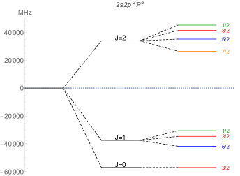
Figure 2: The fine and hyperfine splitting for the $2s2p\,^{3}\!P^{o}$ state. The hf splitting was scaled by a factor of 20.

Because the states ${}^{3}\!S_{1}$, ${}^{1}\!P_{1}$, and ${}^{1}\!D_{2}$ involve only two angular momenta, one can employ the commonly used $A_{J}$ and $B_{J}$ coefficients to represent their hyperfine structure

$$\langle H_{\rm hfs}\rangle_{J} =A_{J}\,\vec{I}\cdot\vec{J}+\frac{B_{J}}{6}\,\frac{3\,(I^{i}\,I^{j})^{(2)}}{I\,(2\,I-1)}\,\frac{3\,(J^{i}\,J^{j})^{(2)}}{J\,(2\,J-1)},$$ (66)

where $\vec{J}$ is the total electronic angular momentum. So, in the case of the $2s3s\,^{3}\!S_{1}$ state, $\vec{J}=\vec{S}$ and

$$A_{1}(^{3}\!S) =a_{1}\,(1+\epsilon)=-332.50(2)\text{ MHz}$$ (67)

$$B_{1}(^{3}\!S) =0\,,$$ (68)

where $\epsilon=0.654\times 10^{-3}$ was taken from Ref. [Puchalski:21]. In the case of the $2s2p\,^{1}\!P_{1}$ state, $\vec{J}=\vec{L}$ and

$$A_{1}(^{1}\!P) =a_{2}=-13.888\,2(7)\text{ MHz}$$ (69)

$$B_{1}(^{1}\!P) =b=0.845\,40(4)\text{ MHz}\,.$$ (70)

Finally for the $2p^{2}\,{}^{1}\!D_{2}$ state, $\vec{J}=\vec{L}$ and

$$A_{2}(^{1}\!D) =a_{2}=-13.964\,0(7)\text{ MHz}$$ (71)

$$B_{2}(^{1}\!D) =b=1.742\,80(9)\text{ MHz}\,.$$ (72)

The calculation of the fine/hyperfine structure for the $2s2p\,^{3}\!P$, $2p^{2}\,{}^{3}\!P^{e}$, and $2s3d\,^{3}\!D$ states requires diagonalization of the effective fine/hyperfine Hamiltonian in Eq. (V). For the $2s3d\,^{3}\!D$ state, the diagonalization reveals that the $a_{1}$ parameter is around three times larger than the parameters $c_{1}$ and $c_{2}$. This makes the interaction of electronic and nuclear spins the dominating one and disqualifies $J$ as a good quantum number. Therefore, one cannot use $A_{J}$ and $B_{J}$ coefficients—instead we present actual values of the fine/hyperfine levels. In addition, to account for the leading relativistic and radiative corrections, the $a_{1}$ parameter is rescaled by the $(1+\epsilon)$ factor, see Eq. (67) and the related discussion in Sec. II.3.2.

Table 4: Centroid energy contributions (in $\mathrm{cm}^{-1}$) relative to the ground $2s^{2}\,{}^{1}\!S$ state for ${}^{9}$Be and comparison with experimental and other theoretical data. The total energy in terms of the ionization potential is also shown at the bottom of the table.

	$2s2p\,^{3}\!P$	$2s2p\,^{1}\!P$	$2s3s\,^{3}\!S$	$2p^{2}\,{}^{1}\!D$	$2p^{2}\,{}^{3}\!P^{e}$	$2s3d\,^{3}\!D$
$m\alpha^{2}$	$21\,968.103(3)$	$42\,554.325(6)$	$52\,075.750(10)$	$56\,862.395(5)$	$59\,667.912(2)$	$62\,046.433(3)$
$m\alpha^{4}$	$13.189(3)$	$12.171(3)$	$5.726(4)$	$21.968(4)$	$30.728(4)$	$8.000(5)$
$m\alpha^{5}$	$-1.06(4)$	$-1.0106(10)$	$-0.46(7)$	$-1.73(5)$	$-2.46(5)$	$-0.61(5)$
$m\alpha^{6}$	$-0.048(10)$	$-0.045(9)$	$-0.021(5)$	$-0.08(2)$	$-0.11(3)$	$-0.027(7)$
Total	$21\,980.18(5)$	$42\,565.441(11)$	$52\,080.99(7)$	$56\,882.55(6)$	$59\,696.07(6)$	$62\,053.79(6)$
Theory (ECG)	$21\,979.4(11)^{e}$
Theory (FCPC)${}^{f}$	$21\,980.85$	$42\,568.80$	$52\,081.09$	$56\,890.9$	$59\,699.8$	$62\,055.25$
Theory (MCHF)${}^{h}$	$22\,099.30$	$42\,710.97$	$52\,080.09$	$56\,945.89$	$59\,793.35$	$62\,165.91$
Experiment	$21\,980.16(8)^{a,g}$	$42\,565.450\,2(10)^{b}$	$52\,080.94(6)^{a}$	$56\,882.547\,4(21)^{c}$	$59\,696.07(5)^{a,g}$	$62\,053.74(6)^{a,g}$
Total $-$ Experiment${}^{d}$	$0.02(5)$	$-0.009(11)$	$0.05(7)$	$0.00(6)$	$0.04(6)$	$0.05(6)$
Total (ionization)	$53\,212.51(5)$	$32\,627.265(11)$	$23\,111.73(5)$	$18\,310.13(5)$	$15\,496.62(6)$	$13\,138.90(5)$
Theory(FCPC)${}^{f}$	$53\,211.22$	$32\,623.27$	$23\,110.98$			$13\,136.8$

${}^{a}$ Johansson [Johansson:62], Kramida et al. [Kramida:20]; ${}^{b}$ Cook et al. [Cook:18]; ${}^{c}$ Cook et al. [Cook:20]; ${}^{d}$ Theoretical uncertainty assumed.; ${}^{e}$ Kedziorski et al.  [Kedziorski:20], averaged over $J$; ${}^{f}$ Chung and Zhu [Chung:93, Zhu:95]; ${}^{g}$ Centroid uncertainty taken as the maximum error from the individual $J$ lines.; ${}^{h}$ Fischer and Tachiev [Fischer:04].