Multi-Source domain adaptation via supervised contrastive learning and confident consistency regularization

Abstract

Multi-Source Unsupervised Domain Adaptation (multi-source UDA) aims to learn a model from several labeled source domains while performing well on a different target domain where only unlabeled data are available at training time. To align source and target features distributions, several recent works use source and target explicit statistics matching such as features moments or class centroids. Yet, these approaches do not guarantee class conditional distributions alignment across domains. In this work, we propose a new framework called Contrastive Multi-Source Domain Adaptation (CMSDA) for multi-source UDA that addresses this limitation. Discriminative features are learned from interpolated source examples via cross entropy minimization and from target examples via consistency regularization and hard pseudo-labeling. Simultaneously, interpolated source examples are leveraged to align source class conditional distributions through an interpolated version of the supervised contrastive loss. This alignment leads to more general and transferable features which further improves the generalization on the target domain. Extensive experiments have been carried out on three standard multi-source UDA datasets where our method reports state-of-the-art results.

1 Introduction

The performances of deep learning models are known to drop when training and testing data have different distributions. This phenomenon, known as Domain Shift, has led to the emergence of the Unsupervised Domain Adaptation (UDA) problem that has been intensively studied over the recent years [Long et al.(2016)Long, Zhu, Wang, and Jordan, Long et al.(2017)Long, Zhu, Wang, and Jordan, Long et al.(2015)Long, Cao, Wang, and Jordan, Tzeng et al.(2014)Tzeng, Hoffman, Zhang, Saenko, and Darrell, Venkateswara et al.(2017)Venkateswara, Eusebio, Chakraborty, and Panchanathan, Zhang et al.(2015)Zhang, Yu, Chang, and Wang, Sun and Saenko(2016), Xie et al.(2018)Xie, Zheng, Chen, and Chen, Kang et al.(2019)Kang, Jiang, Yang, and Hauptmann, Deng et al.(2019)Deng, Luo, and Zhu]. Single-source UDA aims to leverage labeled examples from a source domain and unlabeled examples from a target domain to learn a model that performs well on unseen target examples. In the most practical scenario, to collect as much labeled data as possible, several source domains are considered rather than a single one. In such case, the setting is referred to as multi-source UDA.

To solve the UDA problem, most of the methods learn discriminative features from labeled source data and exploit unlabeled target data to align source and target distributions. Source and target distributions alignment is performed so as to maintain the discriminative power of the model on the target domain. Plethora of UDA methods, in the single-source [Long et al.(2016)Long, Zhu, Wang, and Jordan, Long et al.(2017)Long, Zhu, Wang, and Jordan, Long et al.(2015)Long, Cao, Wang, and Jordan, Tzeng et al.(2014)Tzeng, Hoffman, Zhang, Saenko, and Darrell, Venkateswara et al.(2017)Venkateswara, Eusebio, Chakraborty, and Panchanathan, Zhang et al.(2015)Zhang, Yu, Chang, and Wang] or multi-source settings [Xu et al.(2018)Xu, Chen, Zuo, Yan, and Lin, Zhao et al.(2018)Zhao, Zhang, Wu, Moura, Costeira, and Gordon, Peng et al.(2019)Peng, Bai, Xia, Huang, Saenko, and Wang] have tried to align source and target marginal distributions. However, these methods are susceptible to fail if source and target class conditional distributions are not aligned [Cicek and Soatto(2019)]. Alignment of source and target class conditional distributions can be achieved through adversarial based methods such as [Cicek and Soatto(2019)] but they tend to be cumbersome to train while the alignment of the domains can fail if pseudo labels on target examples are noisy. To align source and target class conditional distributions, [Xie et al.(2018)Xie, Zheng, Chen, and Chen] has proposed to match source and target class centroids. Nevertheless, in order to estimate accurately the true class centroids, batches should be carefully designed to contain enough examples per class while maintaining a well-tuned moving average of centroids. This method assumes also that a single centroid can represent the whole distribution in a class which is a wrong assumption in case of multimodal class distributions.

In this work, to address the problem of multi-source UDA and align efficiently source class conditional distributions, we introduce a new framework named Contrastive Multi-Source Domain Adaptation (CMSDA). CMSDA learns discriminative features on source examples via cross entropy minimization and align class conditional distributions of all source domains through supervised contrastive loss. Source class conditional distributions alignment leads to more general and transferable features for the target domain. In the same time, the model adjusts to the target domain via hard pseudo labeling and consistency regularization. To further enhance the robustness, calibration of our model and enable deeper exploration of each source domain input space, MixUp [Zhang et al.(2018)Zhang, Cisse, Dauphin, and Lopez-Paz] is leveraged on source domains. However, MixUp could be replaced by any other mixing methods such as CutMix [Yun et al.(2019)Yun, Han, Oh, Chun, Choe, and Yoo]. Interpolating source examples from different source domains can even be seen as way to mix source domains styles. Since MixUp is performed on source domains, interpolated versions of the cross entropy and supervised contrastive losses are used in the final objective rather than the standard versions. To sum up, our contributions are the following: (1) we design a novel tailored end-to-end architecture that maps the different domains to a common latent space, and efficiently transfers knowledge learned on source domains to the target domain using recent advances of supervised contrastive learning, semi-supervised learning and mixup training; (2) we show for the first time that supervised contrastive learning and its interpolated extension can be used in the context of domain adaptation for source class conditional distributions alignment leading to higher accuracy for target domains with large domain shift, (3) we report state of the art results on three standard multi-source UDA datasets.

2 Related works

Multi-source UDA. In the multi-source UDA setting, former methods such as MDAN [Zhao et al.(2018)Zhao, Zhang, Wu, Moura, Costeira, and Gordon] have tried to extend a single-source UDA method to the multi-source setting. In MDAN, each source and target marginal distributions are aligned via an adversarial based method  [Ganin and Lempitsky(2015)]. In DCTN [Xu et al.(2018)Xu, Chen, Zuo, Yan, and Lin], an adversarial based method is proposed to align marginally each source with the target and perplexity scores, measuring the possibilities that a target sample belongs to the different source domains, are used to weight predictions of different source classifiers. M³SDA-$\beta$ [Peng et al.(2019)Peng, Bai, Xia, Huang, Saenko, and Wang] uses a two-steps approach combining an ensemble of source classifiers. In the first step, the method aligns marginally each source with the target domain and also each pair of source domains by matching first order moments of features maps channels. In the second step, to enhance distributions alignment, the different source classifiers are trained following an adversarial method [Saito et al.(2018)Saito, Watanabe, Ushiku, and Harada]. CMSS [Yang et al.(2020)Yang, Balaji, Lim, and Shrivastava] exploits an original adversarial approach that selects dynamically the source domains and examples that are the most suitable for aligning source and target distributions. DAEL [Zhou et al.(2020)Zhou, Yang, Qiao, and Xiang] combines a collaborative training of an ensemble of source expert classifiers with hard pseudo labeling and consistency regularization on the target domain. For source examples, robust features are learned by ensuring consistency between the expert source classifier and the ensemble of non-expert source classifiers. For unlabeled target examples, since no expert target classifier is available, consistency is ensured between the most confident source expert classifier and the ensemble of other source expert classifiers. Our method shares some similarities with DAEL as it exploits similar semi-supervised learning techniques to learn on unlabeled target data however, ours adds an additional constraint to align source class conditional distributions. Recent works are also focusing on improving UDA methods by using specific data augmentation. For instance, MixUp has been explored for single source UDA methods  [Wu et al.(2020)Wu, Inkpen, and El-Roby, Xu et al.(2020)Xu, Zhang, Ni, Li, Wang, Tian, and Zhang] but the literature on methods exploiting MixUp for problems such as multi-source UDA and multi-source Domain Generalization is still very sparse [Wang et al.(2020b)Wang, Li, and Kot, Mancini et al.(2020)Mancini, Akata, Ricci, and Caputo]. Our method exploits MixUp but also an interpolated version of the supervised contrastive loss to work with the soft labels produced by this data augmentation. Finally, multi-source UDA methods have also explored other types of approaches [Zhu et al.(2019)Zhu, Zhuang, and Wang, Li et al.(2018)Li, Murias, Major, Dawson, and Carlson, Zhao et al.(2020)Zhao, Wang, Zhang, Gu, Li, Song, Xu, Hu, Chai, and Keutzer, Wang et al.(2020a)Wang, Xu, Ni, and Zhang], different setting [Guo et al.(2018)Guo, Shah, and Barzilay] or other data modalities [Rakshit et al.(2020)Rakshit, Tamboli, Meshram, Banerjee, Roig, and Chaudhuri].

Contrastive learning. Recently, representation learning has known major breakthroughs due to the advance in the field of contrastive learning [Oord et al.(2018)Oord, Li, and Vinyals, Chen et al.(2020)Chen, Kornblith, Norouzi, and Hinton, He et al.(2020)He, Fan, Wu, Xie, and Girshick, Grill et al.(2020)Grill, Strub, Altché, Tallec, Richemond, Buchatskaya, Doersch, Avila Pires, Guo, Gheshlaghi Azar, Piot, kavukcuoglu, Munos, and Valko, Caron et al.(2020)Caron, Misra, Mairal, Goyal, Bojanowski, and Joulin, Chen and He(2020)]. The main idea behind most of contrastive learning methods is that similar examples should share the same representation. For example, in SimCLR [Chen et al.(2020)Chen, Kornblith, Norouzi, and Hinton] the loss enforces pairs of augmented versions of the same image (positives) to have the same representation while having dissimilar representations from all other examples in the batch (negatives). Most recently, the loss used in [Chen et al.(2020)Chen, Kornblith, Norouzi, and Hinton] has been extended for the supervised setting [Khosla et al.(2020)Khosla, Teterwak, Wang, Sarna, Tian, Isola, Maschinot, Liu, and Krishnan]. With the supervised contrastive loss, examples belonging to the same class are pushed closer while examples from different classes are pushed apart. There have been some attempts to adapt contrastive learning in the case of single-source UDA [Kang et al.(2019)Kang, Jiang, Yang, and Hauptmann]. However, supervised contrastive learning has yet to be explored on the multi-source UDA problem and seems a natural and an appropriate approach to align source class conditional distributions.

Semi-supervised learning. To exploit unlabeled examples, common semi-supervised approaches are based either on consistency regularization [Tarvainen and Valpola(2017), Berthelot et al.(2019)Berthelot, Carlini, Goodfellow, Papernot, Oliver, and Raffel, Xie et al.(2020)Xie, Dai, Hovy, Luong, and Le, Mustafa and Mantiuk(2020)] or pseudo labeling [Arazo et al.(2020)Arazo, Ortego, Albert, O’Connor, and McGuinness]. Consistency regularization learns on unlabeled data by relying on the assumption that the model should output similar predictions when perturbed versions of the same image are presented. Hard pseudo-labeling consists of using hard predictions on unlabeled examples as ground truth labels for these examples. Some semi-supervised methods such as FixMatch [Sohn et al.(2020)Sohn, Berthelot, Li, Zhang, Carlini, Cubuk, Kurakin, Zhang, and Raffel] uses both approaches. In FixMatch, strongly and weakly augmented images are generated from the same unlabeled image. The network is then trained to ensure consistency between the prediction on the strongly augmented image and the hard pseudo label obtained on the weakly augmented image. To handle potential false pseudo labels, only confident pseudo-labeled examples contributes to the loss. In our method, these two different kind of approaches are leveraged to learn on the unlabeled target data.

3 CMSDA Framework

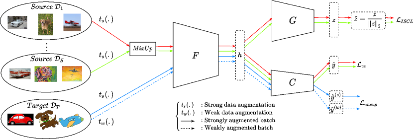
Figure 1: CMSDA framework. CMSDA contains 3 shared components: a features extractor $F$, a projection head $G$ and a classification head $C$. Source examples are strongly augmented via $t_{s}(.)$ and interpolated using MixUp. Target examples are weakly and strongly augmented via $t_{w}(.)$ and $t_{s}(.)$. All examples are fed to $F$ to produce the embeddings $\bm{h}$. In the top branch, source embeddings $\bm{h}$ are given to $G$ to produce the representations $\bm{\tilde{z}}$ which are used to align source class conditional distributions via minimization of $\mathcal{L}_{ISCL}$. In the bottom branch, all embeddings $\bm{h}$ are fed to $C$ to produce probability vectors $\bm{\hat{y}}$, $\bm{\hat{y}^{(s)}}$ and $\bm{\hat{y}^{(w)}}$. These probability vectors are used to learn discriminative features via minimization of $\mathcal{L}_{ce}$ and $\mathcal{L}_{unsup}$.

In the setting of multi-source UDA, we are given $S$ different source domains $\{\mathcal{D}_{1},\ldots,\mathcal{D}_{S}\}$ and one target domain $\mathcal{D}_{T}$. Each of the source domain $\mathcal{D}_{i}$ contains $n_{\mathcal{D}_{i}}$ labeled examples $\{(\bm{x_{j}},\bm{y_{j}})\mid 1\leq j\leq n_{\mathcal{D}_{i}}\}$ while target domain contains $n_{\mathcal{D}_{T}}$ unlabeled examples $\{\bm{x_{j}}\mid 1\leq j\leq n_{\mathcal{D}_{T}}\}$. The goal of multi-source UDA is to learn a robust model from the $S$ labeled source domains $\mathcal{D}_{1},\ldots,\mathcal{D}_{S}$ and the target domain $\mathcal{D}_{T}$ so that it generalizes well on unseen target domain examples.

3.1 Model architecture

Our model architecture (Figure 1) is shared for source and target domains. It is composed of three different parts:

Features extractor. The features extractor $F$ is a convolutional neural network. It takes an input image $\bm{x}\in\mathbb{R}^{H\times W\times 3}$ and returns a features vector $\bm{h}\in\mathbb{R}^{d_{1}}$.

Projection head. The projection head $G$ takes as input the representation $\bm{h}$ and outputs a lower dimensional representation $\bm{z}\in\mathbb{R}^{d_{2}}$ with $d_{1}>d_{2}$. Similarly to [Khosla et al.(2020)Khosla, Teterwak, Wang, Sarna, Tian, Isola, Maschinot, Liu, and Krishnan], $G$ is a multi-layer perceptron consisting in two fully connected layers. The first layer preserves the dimension while the second reduces the dimensions from $d_{1}$ to $d_{2}$. Previous self-supervised contrastive learning methods [He et al.(2020)He, Fan, Wu, Xie, and Girshick, Grill et al.(2020)Grill, Strub, Altché, Tallec, Richemond, Buchatskaya, Doersch, Avila Pires, Guo, Gheshlaghi Azar, Piot, kavukcuoglu, Munos, and Valko, Caron et al.(2020)Caron, Misra, Mairal, Goyal, Bojanowski, and Joulin, Chen and He(2020)] indicate that the use of a batch normalization layer after the first fully connected layer has shown to generate more powerful representations. Following these findings, we include a batch normalization after the first fully connected layer of $G$.

Classification head. The classification head $C$ is responsible for the final predictions. In previous self-supervised [Chen et al.(2020)Chen, Kornblith, Norouzi, and Hinton] or supervised [Khosla et al.(2020)Khosla, Teterwak, Wang, Sarna, Tian, Isola, Maschinot, Liu, and Krishnan] contrastive learning methods, the projection head is usually removed after the training and a linear classifier is fine-tuned on top of the frozen representation $\bm{h}$. Indeed, in practice, $\bm{h}$ provides better representations than $\bm{z}$ for the final classification task. In this study, we follow the same strategy but still investigate this design choice in the experiments. Therefore, $C$ is a single fully connected layer that takes as input the features extractor representation $\bm{h}$ and outputs a probability vector $\bm{\hat{y}}\in[0,1]^{K}$ where $K$ is the number of classes.

3.2 Optimization Strategy

Source domains interpolation with MixUp. MixUp  [Zhang et al.(2018)Zhang, Cisse, Dauphin, and Lopez-Paz] performs data augmentation by creating new examples $(\bm{\tilde{x}},\bm{\tilde{y}})$ as convex combinations of random pairs of examples and their corresponding labels $(\bm{x_{a}},\bm{y_{a}})$ and $(\bm{x_{b}},\bm{y_{b}})$:

$$\begin{cases}\bm{\tilde{x}}=\lambda\bm{x_{a}}+(1-\lambda)\bm{x_{b}}\\ \bm{\tilde{y}}=\lambda\bm{y_{a}}+(1-\lambda)\bm{y_{b}}\end{cases}$$ (1)

where $\lambda\sim Beta(\alpha,\alpha)$. In CMSDA, MixUp is applied on source examples right after strong data augmentation $t_{s}(.)$.

Overall objective. The overall objective includes three different losses: the interpolated cross entropy loss $\mathcal{L}_{ce}$, the interpolated supervised contrastive loss $\mathcal{L}_{ISCL}$ and the unsupervised FixMatch loss $\mathcal{L}_{unsup}$. The final objective minimized by the model can be written:

$$\mathcal{L}=\mathcal{L}_{ce}+\lambda_{1}\mathcal{L}_{ISCL}+\lambda_{2}\mathcal{L}_{unsup}$$ (2)

$\lambda_{1}$ and $\lambda_{2}$ are hyperparameters weighting the contributions of the losses $\mathcal{L}_{ISCL}$ and $\mathcal{L}_{unsup}$.

Interpolated cross-entropy. In order to leverage the interpolated labeled source examples obtained after MixUp, our framework minimizes an interpolated cross entropy denoted $\mathcal{L}_{ce}$. For a single interpolated source example $(\bm{\tilde{x_{i}}},\bm{\tilde{y_{i}}})=(\lambda\bm{x_{a}}+(1-\lambda)\bm{x_{b}},\lambda\bm{y_{a}}+(1-\lambda)\bm{y_{b}})$ with $\bm{\hat{y}}$ the prediction on the example $\bm{\tilde{x_{i}}}$, the interpolated cross entropy per sample denoted $\mathcal{L}_{i}^{ce}$ can be written:

$$\mathcal{L}_{i}^{ce}=H(\lambda\bm{y_{a}}+(1-\lambda)\bm{y_{b}},\bm{\hat{y}})$$ (3)

$H(\bm{p},\bm{q})$ denotes the cross entropy between a reference distribution $\bm{p}$ and an approximated distribution $\bm{q}$. $\mathcal{L}_{ce}$ is then computed by averaging the loss per sample on $N_{S}$ interpolated source examples.

Interpolated supervised contrastive loss. To align source class conditional distributions, supervised contrastive loss (SCL) seems a simple and straightforward option. When minimizing SCL, representations of examples belonging to the same class are pulled together while representations of examples belonging to different classes are pushed away. In the case of multiple source domains, SCL would force learned features to be domain invariant. Given an example $(\bm{x_{i}},\bm{y_{i}})$ with normalized projection head representation $\bm{\tilde{z_{i}}}$, the per sample SCL is defined by:

Here, $T$ corresponds to a temperature hyperparameter, $A(i)$ stands for the anchors set (indexes of examples different than $i$) and $P(i,\bm{y_{i}})$ the positives set (indexes of other examples whose label is equal to $\bm{y_{i}}$).

However, by using MixUp on source examples, we end up with examples with soft labels whereas SCL requires hard labels. Indeed, SCL needs hard labels so that examples with same labels can be identified and be pulled together. To circumvent the soft labels problem raised by MixUp, we instead use an interpolated version of SCL (ISCL) introduced in [Ortego et al.(2020)Ortego, Arazo, Albert, O’Connor, and McGuinness] and minimize it on $N_{S}$ interpolated source examples.

Given an interpolated source example $(\bm{\tilde{x_{i}}},\bm{\tilde{y_{i}}})=(\lambda\bm{x_{a}}+(1-\lambda)\bm{x_{a}},\lambda\bm{y_{a}}+(1-\lambda)\bm{y_{b}})$ with $\bm{\tilde{z_{i}}}$ the normalized projection head representation of the example $\bm{\tilde{x_{i}}}$, the per sample ISCL denoted $\mathcal{L}_{i}^{ISCL}$ is defined by:

$$\mathcal{L}_{i}^{ISCL}=\lambda\mathcal{L}^{SCL}(\bm{\tilde{z_{i}}},\bm{y_{a}})+(1-\lambda)\mathcal{L}^{SCL}(\bm{\tilde{z_{i}}},\bm{y_{b}})$$ (5)

$\mathcal{L}^{SCL}(\bm{\tilde{z_{i}}},\bm{y_{a}})$ ($\mathcal{L}^{SCL}(\bm{\tilde{z_{i}}},\bm{y_{b}})$) stands for the per sample SCL for the example $\bm{x_{i}}$ with label $\bm{y_{a}}$ ($\bm{y_{b}}$). The definition of $P(i,\bm{y_{i}})$ in Equation 4 implies that the examples in $A(i)$ have hard labels. Therefore, as in [Ortego et al.(2020)Ortego, Arazo, Albert, O’Connor, and McGuinness], for each interpolated example in $A(i)$, we consider as hard label the dominant label which is the one associated to the highest mixing coefficients $(\lambda,1-\lambda)$. Finally, $\mathcal{L}_{ISCL}$ is computed by averaging the loss per sample on $N_{S}$ interpolated source examples.

Consistency regularization and hard-pseudo labeling. In our framework, given $N_{T}$ unlabeled examples drawn from the target domain, we apply a weak augmentation $t_{w}(.)$ and a strong augmentation $t_{s}(.)$ on each example to obtain a weakly augmented example $\bm{x^{(w)}}$ and strongly augmented example $\bm{x^{(s)}}$. $\bm{x^{(w)}}$ and $\bm{x^{(s)}}$ are fed to $F$ and $C$ to obtain respectively the predictions $\bm{\hat{y}^{(w)}}$ and $\bm{\hat{y}^{(s)}}$. The hard prediction of the weakly augmented example denoted $\arg\max\bm{\hat{y}^{(w)}}$ is used as a hard pseudo label while we ensure consistency between the predictions on the strongly example $\bm{\hat{y}^{(s)}}$ and the hard pseudo label of the weakly augmented example $\arg\max\bm{\hat{y}^{(w)}}$. As described in Section 2, to discard potential noisy pseudo labels, only pseudo-labeled weakly augmented examples with a maximum predicted probability above some fixed probability threshold $\tau$ contributes to the loss. This corresponds to minimizing the unsupervised loss term of  [Sohn et al.(2020)Sohn, Berthelot, Li, Zhang, Carlini, Cubuk, Kurakin, Zhang, and Raffel] defined by:

$$\mathcal{L}_{unsup}=\displaystyle\dfrac{1}{N_{T}}\sum_{i=1}^{N_{T}}\mathbbm{1}_{\{\max\bm{\hat{y}^{(w)}}>\tau\}}H\left(\arg\max\bm{\hat{y}^{(w)}},\bm{\hat{y}^{(s)}}\right)$$ (6)

4 Experiments

4.1 Evaluation

We evaluate and compare our method on three standard multi-source UDA datasets: DomainNet, MiniDomainNet and Office-Home. For each dataset and target domain, two standard baselines commonly used in the context of multi-source UDA [Xu et al.(2018)Xu, Chen, Zuo, Yan, and Lin, Peng et al.(2019)Peng, Bai, Xia, Huang, Saenko, and Wang, Yang et al.(2020)Yang, Balaji, Lim, and Shrivastava, Zhou et al.(2020)Zhou, Yang, Qiao, and Xiang] have been added: Source-only and Oracle. Source-only represents a model trained only on source examples with standard cross-entropy whereas Oracle represents a model trained with labeled target examples. Performances on MiniDomainNet and DomainNet are averaged over three runs with different random seeds. The performances of our method along with the compared multi-source UDA methods for the datasets DomainNet, MiniDomainNet and Office-Home are respectively reported on Table 1, Table 2 and Table 3. For easier interpretation, first and second best methods are respectively highlighted in bold red and italic blue. Datasets information and implementation details can be found in the supplementary material.

DomainNet. Our method achieves the best performance with $50.42\%$ average accuracy which is $+1.72\%$ gain over previous state of the art. Overall, our method reports the best performances on 4 out of 6 target domains and the second best performance on one of the two other target domains. On the Quickdraw domain, our framework achieves the best performance by a large margin $(+2.40\%)$ compared to the second best method (SImpAl). On this challenging target domain, SImpaL, CMSS, LtC-MSDA and our method are the only ones that are not subject to negative transfer [Pan and Yang(2009)] (lower performances than the baseline Source-only). This indicates that our method is able to work even for complex target domains.

MiniDomainNet. Our method achieves the best overall accuracy with $61.90\%$, the best accuracy on 3 out of 4 target domains and the second best on the last domain.

Office-Home. Our method achieves the best overall accuracy with $76.60\%$. More specifically, CMSDA obtains the best/second best accuracies on 2 out of 4 target domains and competitive results on the two other target domains.

Target domain Methods Clp Inf Pnt Qdr Rel Skt Avg Source-only [Zhou et al.(2020)Zhou, Yang, Qiao, and Xiang] $47.60\pm 0.52$ $13.00\pm 0.41$ $38.10\pm 0.45$ $13.30\pm 0.39$ $51.90\pm 0.85$ $33.70\pm 0.54$ $32.90$ Oracle [Zhou et al.(2020)Zhou, Yang, Qiao, and Xiang] $69.30\pm 0.37$ $34.50\pm 0.42$ $66.30\pm 0.67$ $66.80\pm 0.51$ $80.10\pm 0.59$ $60.70\pm 0.48$ $63.00$ DANN [Ganin et al.(2016)Ganin, Ustinova, Ajakan, Germain, Larochelle, Laviolette, Marchand, and Lempitsky] $45.50\pm 0.59$ $13.10\pm 0.41$ $37.00\pm 0.69$ $13.20\pm 0.77$ $48.90\pm 0.65$ $31.80\pm 0.62$ $32.60$ DCTN [Xu et al.(2018)Xu, Chen, Zuo, Yan, and Lin] $48.60\pm 0.73$ $23.50\pm 0.59$ $48.80\pm 0.63$ $7.20\pm 0.46$ $53.50\pm 0.56$ $47.30\pm 0.47$ $38.20$ MCD [Saito et al.(2018)Saito, Watanabe, Ushiku, and Harada] $54.30\pm 0.64$ $22.10\pm 0.70$ $45.70\pm 0.63$ $7.60\pm 0.49$ $58.40\pm 0.65$ $43.50\pm 0.57$ $38.50$ M3SDA-$\beta$ [Peng et al.(2019)Peng, Bai, Xia, Huang, Saenko, and Wang] $58.60\pm 0.53$ $26.00\pm 0.89$ $52.30\pm 0.55$ $6.30\pm 0.58$ $62.27\pm 0.51$ $49.50\pm 0.76$ $42.60$ CMSS [Yang et al.(2020)Yang, Balaji, Lim, and Shrivastava] $64.20\pm 0.18$ $\mathit{28.00\pm 0.20}$ $53.60\pm 0.39$ $16.00\pm 0.12$ $63.40\pm 0.21$ $53.80\pm 0.35$ $46.50$ LtC$-$MSDA [Wang et al.(2020a)Wang, Xu, Ni, and Zhang] $63.10\pm 0.50$ $\bm{28.70\pm 0.70}$ $56.10\pm 0.50$ $16.30\pm 0.50$ $66.10\pm 0.60$ $53.80\pm 0.60$ $47.40$ SImpAl101 [Venkat et al.(2021)Venkat, Kundu, Singh, Revanur, and Babu] $66.40\pm 0.80$ $26.50\pm 0.50$ $56.60\pm 0.70$ $\mathit{18.90\pm 0.80}$ $\mathit{68.00\pm 0.50}$ $55.50\pm 0.30$ $48.60$ DAEL [Zhou et al.(2020)Zhou, Yang, Qiao, and Xiang] $\mathit{70.80\pm 0.14}$ $26.50\pm 0.13$ $\mathit{57.40\pm 0.28}$ $12.20\pm 0.70$ $65.00\pm 0.23$ $\bm{60.60\pm 0.25}$ $\mathit{48.70}$ Ours $\bm{70.95\pm 0.23}$ $26.58\pm 0.34$ $\bm{57.56\pm 0.08}$ $\bm{21.30\pm 0.11}$ $\bm{68.12\pm 0.22}$ $\mathit{59.48\pm 0.07}$ $\bm{50.42}$ Table 1: Accuracy (%) on DomainNet (Clp: Clipart, Inf: Infograph, Pnt: Painting, Qdr: Quickdraw, Rel: Real, Skt: Sketch, Avg: Average).

Target domain Methods Clp Pnt Rel Skt Avg Source-only [Zhou et al.(2020)Zhou, Yang, Qiao, and Xiang] $63.44\pm 0.76$ $49.92\pm 0.71$ $61.54\pm 0.08$ $44.12\pm 0.31$ $54.76$ Oracle [Zhou et al.(2020)Zhou, Yang, Qiao, and Xiang] $72.59\pm 0.30$ $60.53\pm 0.74$ $80.47\pm 0.34$ $63.44\pm 0.15$ $69.26$ DANN [Ganin et al.(2016)Ganin, Ustinova, Ajakan, Germain, Larochelle, Laviolette, Marchand, and Lempitsky] $65.55\pm 0.34$ $46.27\pm 0.71$ $58.68\pm 0.64$ $47.88\pm 0.54$ $54.60$ DCTN [Xu et al.(2018)Xu, Chen, Zuo, Yan, and Lin] $62.06\pm 0.60$ $48.79\pm 0.52$ $58.85\pm 0.55$ $48.25\pm 0.32$ $54.49$ MCD [Saito et al.(2018)Saito, Watanabe, Ushiku, and Harada] $62.91\pm 0.67$ $45.77\pm 0.45$ $57.57\pm 0.33$ $45.88\pm 0.67$ $53.03$ M3SDA-$\beta$ [Peng et al.(2019)Peng, Bai, Xia, Huang, Saenko, and Wang] $64.18\pm 0.27$ $49.05\pm 0.16$ $57.70\pm 0.24$ $49.21\pm 0.34$ $55.03$ MME [Saito et al.(2019)Saito, Kim, Sclaroff, Darrell, and Saenko] $68.09\pm 0.16$ $47.14\pm 0.32$ $63.33\pm 0.16$ $43.50\pm 0.47$ $55.52$ DAEL [Zhou et al.(2020)Zhou, Yang, Qiao, and Xiang] $\mathit{69.95\pm 0.52}$ $\bm{55.13\pm 0.78}$ $\mathit{66.11\pm 0.14}$ $\mathit{55.72\pm 0.79}$ $\mathit{61.73}$ Ours $\bm{71.38\pm 0.65}$ $\mathit{53.76\pm 0.71}$ $\bm{66.23\pm 0.08}$ $\bm{56.24\pm 0.67}$ $\bm{61.90}$ Table 2: Accuracy (%) on MiniDomainNet (Clp: Clipart, Pnt: Painting, Rel: Real, Skt: Sketch, Avg: Average). Target domain Methods Art Clp Pct Rel Avg Source-only [Wen et al.(2020)Wen, Greiner, and Schuurmans] $58.02$ $57.29$ $74.26$ $77.98$ $66.89$ Oracle [Wen et al.(2020)Wen, Greiner, and Schuurmans] $71.19$ $79.16$ $90.66$ $85.60$ $81.65$ M3SDA-$\beta$ [Peng et al.(2019)Peng, Bai, Xia, Huang, Saenko, and Wang] $64.05$ $62.79$ $76.21$ $78.63$ $70.42$ SImpAl50 [Venkat et al.(2021)Venkat, Kundu, Singh, Revanur, and Babu] $70.80$ $56.30$ $80.20$ $81.50$ $72.20$ MFSAN [Zhu et al.(2019)Zhu, Zhuang, and Wang] $\bm{72.10}$ $62.00$ $80.30$ $81.80$ $74.10$ MDAN [Zhao et al.(2018)Zhao, Zhang, Wu, Moura, Costeira, and Gordon] $68.14$ $67.04$ $81.03$ $82.79$ $74.75$ MDMN [Li et al.(2018)Li, Murias, Major, Dawson, and Carlson] $68.67$ $\mathit{67.75}$ $81.37$ $\mathit{83.32}$ $75.28$ DARN [Wen et al.(2020)Wen, Greiner, and Schuurmans] $\mathit{70.00}$ $\bm{68.42}$ $\mathit{82.75}$ $\bm{83.88}$ $\mathit{76.26}$ Ours $\mathit{71.49}$ $67.72$ $\bm{84.19}$ $82.99$ $\bm{76.60}$ Table 3: Accuracy (%) on Office-Home (Art: Art, Clp: Clipart, Pct: Product, Rel: Real-World, Avg: Average).

Source class conditional distributions alignment. To assess the efficiency of $\mathcal{L}_{ISCL}$ on source class conditional distributions alignment, CMSDA has been trained separately with $\mathcal{L}_{ce}$ and $\mathcal{L}_{ce}+\lambda_{1}\mathcal{L}_{ISCL}$ for each (sources, target) possible combination. Then, the Calinski-Harabasz index (CH-index) [Caliński and Harabasz(1974)], a clustering quality metric, has been computed on the source examples embedding $\bm{h}$. Using CH-index, we could identify and evaluate if the class conditional distributions from the different source domains are well aligned. For each (sources, target) combination, the CH-indexes with and without $\mathcal{L}_{ISCL}$ are reported on Figure 2a. As expected, when $\mathcal{L}_{ISCL}$ is used in the final objective, the CH-index increases systematically. This suggests that $\mathcal{L}_{ISCL}$ aligns efficiently source class conditional distributions while keeping discrimative features.

4.2 Ablation study

Target domain Clp Pnt Rel Skt $\mathcal{L}_{ce}$ $3.76$ $4.08$ $3.66$ $3.97$ $\mathcal{L}_{ce}+\lambda_{1}\mathcal{L}_{ISCL}$ $\bm{4.02}$ $\bm{4.47}$ $\bm{3.92}$ $\bm{4.26}$ (a) Target domain Input Clp Pnt Rel Skt Avg $\bm{z}$ $69.36$ $53.03$ $66.03$ $56.04$ $61.11$ $\bm{h}$ $71.38$ $53.76$ $66.23$ $56.24$ $61.90$ (b) Target domain Mixup Clp Pnt Rel Skt Avg w/o Mixup $70.32$ $51.75$ $64.92$ $51.11$ $59.52$ w Mixup $\bm{71.38}$ $\bm{53.76}$ $\bm{66.23}$ $\bm{56.24}$ $\bm{61.90}$ (c)

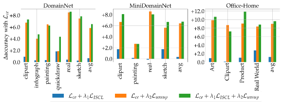
(d)

Figure 2: CH indexes for each combination of target and sources domains of MiniDomainNet considering only the source embeddings $\bm{h}$ with or without $\mathcal{L}_{ISCL}$ (a), performances in terms of accuracy on MiniDomainNet with classification on $\bm{h}$ or $\bm{z}$ embeddings (b), with or without MixUp and interpolated losses (c), $\Delta$accuracy compared to standard $\mathcal{L}_{ce}$ for different combination of losses (d).

Classification on $\bm{h}$ or $\bm{z}$. Similarly to self-supervised methods such as [Chen et al.(2020)Chen, Kornblith, Norouzi, and Hinton], we have investigated the behavior of our model when the classification head takes as input the features extractor representation $\bm{h}$ or the projection head representation $\bm{z}$. For each target domain of MiniDomainNet, the framework has been trained by either feeding $\bm{h}$ or $\bm{z}$ to the classification head. The accuracies obtained on the different target domains of MiniDomainNet are reported in Figure 2b. Using the representation $\bm{z}$ instead of $\bm{h}$ leads to little lower performances on every target domain but performances remain competitive to other multi-source UDA methods. For the Clipart domain, using $\bm{z}$ results in a $2\%$ accuracy drop. These performances discrepancies are in adequacy with the findings of [Chen et al.(2020)Chen, Kornblith, Norouzi, and Hinton] arguing that $\bm{h}$ usually provides better representations for the final classification task. Therefore, even if performances are quite comparable, we recommend feeding $\bm{h}$ to the classification head $C$.

MixUp and interpolated losses. To assess the contributions of MixUp and interpolated losses on CMSDA performances, we have trained two different versions of the framework. In the first version, MixUp is removed while standard versions of the cross entropy and supervised contrastive losses are used. Conversely, in the second version, MixUp is applied on source examples and interpolated versions of the cross entropy and the supervised contrastive losses are used. Accuracies for these two versions and for each target domain of MiniDomainNet are reported on Figure 2c. It suggests that MixUp combined with the interpolated losses brings a significant gain of performances. The average accuracy gain is more than $2\%$. We believe that MixUp applied on examples from different source domains can be seen as a way to mix source domains style which serves as an efficient data augmentation to learn domain invariant features. Additionally, we think that the combination of MixUp and interpolated cross entropy improves the model calibration and robustness on out-of-distribution data. This enables cleaner pseudo-labels for target examples.

Loss ablation. To highlight the influence of each loss on the overall performances, CMSDA has been trained with different combinations of the losses $\mathcal{L}_{ce}$, $\mathcal{L}_{ISCL}$ and $\mathcal{L}_{unsup}$. For this experiment, the hyperparameters remain unchanged. For each dataset and each combination of losses, we report on Figure 2d the gain/loss in terms of accuracy compared to minimizing only $\mathcal{L}_{ce}$. When $\mathcal{L}_{ISCL}$ is combined with $\mathcal{L}_{ce}$ (blue bars), it has in average a positive impact ($0.68\%$, $0.87\%$ and $1.19\%$ respectively for DomainNet (DN), MiniDomainNet (MDN) and OfficeHome (OH)). More specifically, it brings significant gains for target domains with large domain shift (DN-quickdraw: $+1.85\%$, MDN-sketch:$+1.75\%$ or OH-Real World: $+2.75\%$). Even if in some rare cases, such as MDN-real, $\mathcal{L}_{ISCL}$ leads to a very small loss of accuracy, its overall contribution is beneficial. When $\mathcal{L}_{unsup}$ is added to $\mathcal{L}_{ce}$ (orange bars), performances are systematically improved. In general, $\mathcal{L}_{unsup}$ contribution is higher than $\mathcal{L}_{ISCL}$. This is consistent with the performances gap usually observed between methods that do exploit target data (multi-source UDA) and the ones that do not (multi-source Domain Generalization). Additionally, when $\mathcal{L}_{ISCL}$ is combined to $\mathcal{L}_{ce}$ and $\mathcal{L}_{unsup}$ (green bars), the performances are often enhanced and especially on the most challenging target domains (DN-quickdraw: $+2.48\%$, DN-infograph: $+0.75\%$, MDN-sketch: $+1.01\%$). The accuracy gains of $\mathcal{L}_{ISCL}$ and $\mathcal{L}_{unsup}$ seem to be additive suggesting that their contributions are independent. These observations prove the usefulness of each loss and their independent contributions to the overall framework.

4.3 Sensitivity to hyperparameters

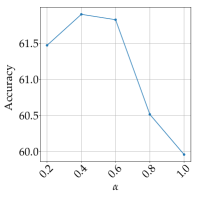
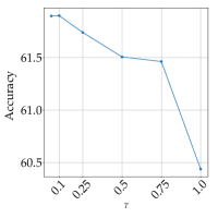
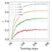
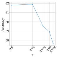
(a)	(b)	(c)	(d)

Figure 3: Averaged accuracy (%) on MiniDomainNet with respect to $\alpha$  (a); $T$ (b); $\tau$ (d). Ratio $r$ of target examples contributing to $\mathcal{L}_{unsup}$ with respect to $\tau$ (c).

In this section, we assess the behavior of the model with respect to its hyperparameters $\alpha$, $T$, and $\tau$. Experiments about $\lambda_{1}$ and $\lambda_{2}$ are included in the supplementary material.

MixUp hyperparameter $\alpha$. In Mixup [Zhang et al.(2018)Zhang, Cisse, Dauphin, and Lopez-Paz], the interpolation parameter $\lambda\in[0,1]$ is drawn such that $\lambda\sim Beta(\alpha,\alpha)$. $\alpha$ controls the interpolation strength. Too low $\alpha$ usually lead to weak regularization while too high $\alpha$ lead to too strong regularization resulting in underfitting and under-confident models [Zhang et al.(2018)Zhang, Cisse, Dauphin, and Lopez-Paz, Thulasidasan et al.(2019)Thulasidasan, Chennupati, Bilmes, Bhattacharya, and Michalak]. We have investigated how $\alpha$ impacts the performances by training the framework with different $\alpha$ and for each target domain of MiniDomainNet. The average accuracy over the target domains with respect to $\alpha$ is reported on Figure 3a. Performances are quite stable for $\alpha\in[0.2,0.6]$ but start decreasing for $\alpha>0.6$, validating the observations made in  [Zhang et al.(2018)Zhang, Cisse, Dauphin, and Lopez-Paz, Thulasidasan et al.(2019)Thulasidasan, Chennupati, Bilmes, Bhattacharya, and Michalak]. $\alpha=0.4$ leads to the best accuracy. To work on other datasets, we suggest $\alpha=0.4$ as a starting point.

Temperature $T$. The temperature hyperparameter $T$ is known to have a crucial role in self-supervised/supervised contrastive learning methods [Chen et al.(2020)Chen, Kornblith, Norouzi, and Hinton, Khosla et al.(2020)Khosla, Teterwak, Wang, Sarna, Tian, Isola, Maschinot, Liu, and Krishnan]. Setting $T$ properly can result in a non negligible gain of performances [Khosla et al.(2020)Khosla, Teterwak, Wang, Sarna, Tian, Isola, Maschinot, Liu, and Krishnan]. According to [Wang and Liu(2020)], selecting the optimal $T$ is a compromise between uniformity and tolerance. Uniformity corresponds to the capacity of the representations $\bm{\tilde{z}}$ to be uniformly distributed over the sphere while tolerance describes how close the representations are for examples in the same class. Uniformity has known to be important to learn separable features however high uniformity induces a decrease of tolerance [Wang and Liu(2020)]. $T\rightarrow 0$ tends to encourage uniformity whereas $T\rightarrow+\infty$ promotes tolerance. To evaluate the effect of the temperature $T$ on the performances, we have trained our model with different $T$ and for each target domain of MiniDomainNet. The average accuracy over the target domains with respect to $T$ is reported on Figure 3b. It seems that our framework benefits from lower temperatures. Indeed, for $T\in[0.05,0.1]$, the performances are quite stable and reach the maximum for $T=0.1$. For $T>0.1$, the accuracy begins to decrease slowly until $T=0.75$ and then it drops. Overall, for multi source UDA, our experiments suggest that uniformity is more important than tolerance however too low temperatures ($T<0.05$) might as well impact negatively the model performances. We suggest to use a temperature $T=0.1$ for further experiments on different datasets.

FixMatch probability threshold $\tau$. In semi-supervised problems, including false pseudo-labeled examples into the training could lead to lower performance [Arazo et al.(2020)Arazo, Ortego, Albert, O’Connor, and McGuinness]. In $\mathcal{L}_{unsup}$, $\tau$ addresses this problem by discarding non confident pseudo-labeled examples. More specifically, pseudo-labeled examples whose maximum predicted probability is below $\tau$ do not contribute to $\mathcal{L}_{unsup}$. To illustrate the trade off between the number of target pseudo labels used by CMSDA, on Figure 3c and for the target domain Clipart of MiniDomainNet, we have plotted for different values of $\tau$ the ratio of target examples $r$ that contribute to the loss $\mathcal{L}_{unsup}$. $r$ is defined as follows:

$$r=\dfrac{\displaystyle\sum_{i=1}^{N_{T}}\mathbbm{1}_{\{\max\bm{\hat{y}_{i}^{(w)}}>\tau\}}}{N_{T}}$$ (7)

Figure 3c reveals that for any value $\tau$, as the training progresses, the model gets more and more confident predictions resulting in an increase of $r$. A second observation is that when $\tau$ is set too low ($\tau=0.9$), $r$ is in average high at the end of training $(r\sim 77\%)$ whereas Oracle reaches only $72.59\%$ accuracy. This suggests that false pseudo-labeled target examples contributes to $\mathcal{L}_{unsup}$. On the contrary, when $\tau$ is set too high ($\tau=0.999$), $r$ is in average very low at the end of training $(r\simeq 0.02)$. This indicates that a lot of correct pseudo-labeled target examples have been discarded. To evaluate the effect of $\tau$ on the performances, CMSDA has been trained with different $\tau$ values for each target domain of MiniDomainNet, while the rest of hyperparameters remain unchanged. The average accuracy over target domains with respect to $\tau$ is reported in Figure 3d. Performances are stable when choosing $\tau\in[0.9,0.95]$. $\tau=0.95$ leads to the highest average accuracy. For $\tau<0.95$, false pseudo labels contribute to $\mathcal{L}_{unsup}$ resulting in a small drop of accuracy. For $\tau>0.95$, as $\tau$ increases, more and more correct pseudo-labeled examples are discarded and performances start to drop.

5 Conclusion

In this work, we have introduced a new framework combining recent advances in supervised contrastive learning and semi-supervised learning to address the problem of multi-source UDA. Our framework, through supervised contrastive learning, is able to align source class conditional distributions resulting in more robust and universal features for the target domain. Simultaneously, the model adjusts to the target domain via hard pseudo labeling and consistency regularization on target examples. Our framework has been evaluated on $3$ datasets commonly used for multi-source UDA and has reported superior results over previous state-of-the-art methods with robust results on complex domain where negative transfer can occur.

In future research, we plan to explore the use of supervised contrastive learning on both source and pseudo-labeled target examples so as to align source and target conditional distributions all together. Additionally, we believe that data augmentation strategies usually designed for domain generalization (MixStyle [Zhou et al.(2021)Zhou, Yang, Qiao, and Xiang], Fourier Based Augmentation [Xu et al.(2021)Xu, Zhang, Zhang, Wang, and Tian]) and conditional normalizations could provide interesting directions for our future work.

References

- [Arazo et al.(2020)Arazo, Ortego, Albert, O’Connor, and McGuinness] Eric Arazo, Diego Ortego, Paul Albert, Noel E O’Connor, and Kevin McGuinness. Pseudo-labeling and confirmation bias in deep semi-supervised learning. In 2020 International Joint Conference on Neural Networks (IJCNN), pages 1–8. IEEE, 2020.
- [Berthelot et al.(2019)Berthelot, Carlini, Goodfellow, Papernot, Oliver, and Raffel] David Berthelot, Nicholas Carlini, Ian Goodfellow, Nicolas Papernot, Avital Oliver, and Colin A Raffel. Mixmatch: A holistic approach to semi-supervised learning. In H. Wallach, H. Larochelle, A. Beygelzimer, F. d'Alché-Buc, E. Fox, and R. Garnett, editors, Advances in Neural Information Processing Systems, volume 32. Curran Associates, Inc., 2019.
- [Caliński and Harabasz(1974)] Tadeusz Caliński and Jerzy Harabasz. A dendrite method for cluster analysis. Communications in Statistics-theory and Methods, 3(1):1–27, 1974.
- [Caron et al.(2020)Caron, Misra, Mairal, Goyal, Bojanowski, and Joulin] Mathilde Caron, Ishan Misra, Julien Mairal, Priya Goyal, Piotr Bojanowski, and Armand Joulin. Unsupervised learning of visual features by contrasting cluster assignments. In H. Larochelle, M. Ranzato, R. Hadsell, M. F. Balcan, and H. Lin, editors, Advances in Neural Information Processing Systems, volume 33, pages 9912–9924. Curran Associates, Inc., 2020.
- [Chen et al.(2020)Chen, Kornblith, Norouzi, and Hinton] Ting Chen, Simon Kornblith, Mohammad Norouzi, and Geoffrey Hinton. A simple framework for contrastive learning of visual representations. In International conference on machine learning, pages 1597–1607. PMLR, 2020.
- [Chen and He(2020)] Xinlei Chen and Kaiming He. Exploring simple siamese representation learning. arXiv preprint arXiv:2011.10566, 2020.
- [Cicek and Soatto(2019)] Safa Cicek and Stefano Soatto. Unsupervised domain adaptation via regularized conditional alignment. In Proceedings of the IEEE/CVF International Conference on Computer Vision, pages 1416–1425, 2019.
- [Deng et al.(2019)Deng, Luo, and Zhu] Zhijie Deng, Yucen Luo, and Jun Zhu. Cluster alignment with a teacher for unsupervised domain adaptation. In 2019 IEEE/CVF International Conference on Computer Vision (ICCV), pages 9944–9953, 2019.
- [Ganin and Lempitsky(2015)] Yaroslav Ganin and Victor Lempitsky. Unsupervised domain adaptation by backpropagation. In International conference on machine learning, pages 1180–1189. PMLR, 2015.
- [Ganin et al.(2016)Ganin, Ustinova, Ajakan, Germain, Larochelle, Laviolette, Marchand, and Lempitsky] Yaroslav Ganin, Evgeniya Ustinova, Hana Ajakan, Pascal Germain, Hugo Larochelle, François Laviolette, Mario Marchand, and Victor Lempitsky. Domain-adversarial training of neural networks. The journal of machine learning research, 17(1):2096–2030, 2016.
- [Grill et al.(2020)Grill, Strub, Altché, Tallec, Richemond, Buchatskaya, Doersch, Avila Pires, Guo, Gheshlaghi Azar, Piot, kavukcuoglu, Munos, and Valko] Jean-Bastien Grill, Florian Strub, Florent Altché, Corentin Tallec, Pierre Richemond, Elena Buchatskaya, Carl Doersch, Bernardo Avila Pires, Zhaohan Guo, Mohammad Gheshlaghi Azar, Bilal Piot, koray kavukcuoglu, Remi Munos, and Michal Valko. Bootstrap your own latent - a new approach to self-supervised learning. In H. Larochelle, M. Ranzato, R. Hadsell, M. F. Balcan, and H. Lin, editors, Advances in Neural Information Processing Systems, volume 33, pages 21271–21284. Curran Associates, Inc., 2020.
- [Guo et al.(2018)Guo, Shah, and Barzilay] Jiang Guo, Darsh J Shah, and Regina Barzilay. Multi-source domain adaptation with mixture of experts. arXiv preprint arXiv:1809.02256, 2018.
- [He et al.(2020)He, Fan, Wu, Xie, and Girshick] Kaiming He, Haoqi Fan, Yuxin Wu, Saining Xie, and Ross Girshick. Momentum contrast for unsupervised visual representation learning. In Proceedings of the IEEE/CVF Conference on Computer Vision and Pattern Recognition, pages 9729–9738, 2020.
- [Kang et al.(2019)Kang, Jiang, Yang, and Hauptmann] Guoliang Kang, Lu Jiang, Yi Yang, and Alexander G Hauptmann. Contrastive adaptation network for unsupervised domain adaptation. In Proceedings of the IEEE/CVF Conference on Computer Vision and Pattern Recognition, pages 4893–4902, 2019.
- [Khosla et al.(2020)Khosla, Teterwak, Wang, Sarna, Tian, Isola, Maschinot, Liu, and Krishnan] Prannay Khosla, Piotr Teterwak, Chen Wang, Aaron Sarna, Yonglong Tian, Phillip Isola, Aaron Maschinot, Ce Liu, and Dilip Krishnan. Supervised contrastive learning. In H. Larochelle, M. Ranzato, R. Hadsell, M. F. Balcan, and H. Lin, editors, Advances in Neural Information Processing Systems, volume 33, pages 18661–18673. Curran Associates, Inc., 2020.
- [Li et al.(2018)Li, Murias, Major, Dawson, and Carlson] Yitong Li, Michael Murias, Samantha Major, Geraldine Dawson, and David E Carlson. Extracting relationships by multi-domain matching. In Proceedings of the 32nd International Conference on Neural Information Processing Systems, pages 6799–6810, 2018.
- [Long et al.(2015)Long, Cao, Wang, and Jordan] Mingsheng Long, Yue Cao, Jianmin Wang, and Michael Jordan. Learning transferable features with deep adaptation networks. In International conference on machine learning, pages 97–105. PMLR, 2015.
- [Long et al.(2016)Long, Zhu, Wang, and Jordan] Mingsheng Long, Han Zhu, Jianmin Wang, and Michael I Jordan. Unsupervised domain adaptation with residual transfer networks. arXiv preprint arXiv:1602.04433, 2016.
- [Long et al.(2017)Long, Zhu, Wang, and Jordan] Mingsheng Long, Han Zhu, Jianmin Wang, and Michael I Jordan. Deep transfer learning with joint adaptation networks. In International conference on machine learning, pages 2208–2217. PMLR, 2017.
- [Mancini et al.(2020)Mancini, Akata, Ricci, and Caputo] Massimiliano Mancini, Zeynep Akata, Elisa Ricci, and Barbara Caputo. Towards recognizing unseen categories in unseen domains. In Computer Vision–ECCV 2020: 16th European Conference, Glasgow, UK, August 23–28, 2020, Proceedings, Part XXIII 16, pages 466–483. Springer, 2020.
- [Mustafa and Mantiuk(2020)] Aamir Mustafa and Rafal K. Mantiuk. Transformation Consistency Regularization- A Semi-Supervised Paradigm for Image-to-Image Translation. In Computer Vision – ECCV 2020, pages 599–615, July 2020.
- [Oord et al.(2018)Oord, Li, and Vinyals] Aaron van den Oord, Yazhe Li, and Oriol Vinyals. Representation learning with contrastive predictive coding. arXiv preprint arXiv:1807.03748, 2018.
- [Ortego et al.(2020)Ortego, Arazo, Albert, O’Connor, and McGuinness] Diego Ortego, Eric Arazo, Paul Albert, Noel E O’Connor, and Kevin McGuinness. Multi-objective interpolation training for robustness to label noise. arXiv preprint arXiv:2012.04462, 2020.
- [Pan and Yang(2009)] Sinno Jialin Pan and Qiang Yang. A survey on transfer learning. IEEE Transactions on knowledge and data engineering, 22(10):1345–1359, 2009.
- [Peng et al.(2019)Peng, Bai, Xia, Huang, Saenko, and Wang] Xingchao Peng, Qinxun Bai, Xide Xia, Zijun Huang, Kate Saenko, and Bo Wang. Moment matching for multi-source domain adaptation. In Proceedings of the IEEE/CVF International Conference on Computer Vision, pages 1406–1415, 2019.
- [Rakshit et al.(2020)Rakshit, Tamboli, Meshram, Banerjee, Roig, and Chaudhuri] Sayan Rakshit, Dipesh Tamboli, Pragati Shuddhodhan Meshram, Biplab Banerjee, Gemma Roig, and Subhasis Chaudhuri. Multi-source open-set deep adversarial domain adaptation. In European Conference on Computer Vision, pages 735–750. Springer, 2020.
- [Saito et al.(2018)Saito, Watanabe, Ushiku, and Harada] Kuniaki Saito, Kohei Watanabe, Yoshitaka Ushiku, and Tatsuya Harada. Maximum classifier discrepancy for unsupervised domain adaptation. In Proceedings of the IEEE conference on computer vision and pattern recognition, pages 3723–3732, 2018.
- [Saito et al.(2019)Saito, Kim, Sclaroff, Darrell, and Saenko] Kuniaki Saito, Donghyun Kim, Stan Sclaroff, Trevor Darrell, and Kate Saenko. Semi-supervised domain adaptation via minimax entropy. In Proceedings of the IEEE/CVF International Conference on Computer Vision, pages 8050–8058, 2019.
- [Sohn et al.(2020)Sohn, Berthelot, Li, Zhang, Carlini, Cubuk, Kurakin, Zhang, and Raffel] Kihyuk Sohn, David Berthelot, Chun-Liang Li, Zizhao Zhang, Nicholas Carlini, Ekin D Cubuk, Alex Kurakin, Han Zhang, and Colin Raffel. Fixmatch: Simplifying semi-supervised learning with consistency and confidence. arXiv preprint arXiv:2001.07685, 2020.
- [Sun and Saenko(2016)] Baochen Sun and Kate Saenko. Deep coral: Correlation alignment for deep domain adaptation. In Computer Vision - ECCV 2016 Workshops, pages 443–450. Springer, 2016.
- [Tarvainen and Valpola(2017)] Antti Tarvainen and Harri Valpola. Mean teachers are better role models: Weight-averaged consistency targets improve semi-supervised deep learning results. In I. Guyon, U. V. Luxburg, S. Bengio, H. Wallach, R. Fergus, S. Vishwanathan, and R. Garnett, editors, Advances in Neural Information Processing Systems, volume 30. Curran Associates, Inc., 2017.
- [Thulasidasan et al.(2019)Thulasidasan, Chennupati, Bilmes, Bhattacharya, and Michalak] Sunil Thulasidasan, Gopinath Chennupati, Jeff Bilmes, Tanmoy Bhattacharya, and Sarah Michalak. On mixup training: Improved calibration and predictive uncertainty for deep neural networks. arXiv preprint arXiv:1905.11001, 2019.
- [Tzeng et al.(2014)Tzeng, Hoffman, Zhang, Saenko, and Darrell] Eric Tzeng, Judy Hoffman, Ning Zhang, Kate Saenko, and Trevor Darrell. Deep domain confusion: Maximizing for domain invariance. arXiv preprint arXiv:1412.3474, 2014.
- [Venkat et al.(2021)Venkat, Kundu, Singh, Revanur, and Babu] Naveen Venkat, Jogendra Nath Kundu, Durgesh Kumar Singh, Ambareesh Revanur, and R Venkatesh Babu. Your classifier can secretly suffice multi-source domain adaptation. arXiv preprint arXiv:2103.11169, 2021.
- [Venkateswara et al.(2017)Venkateswara, Eusebio, Chakraborty, and Panchanathan] Hemanth Venkateswara, Jose Eusebio, Shayok Chakraborty, and Sethuraman Panchanathan. Deep hashing network for unsupervised domain adaptation. In Proceedings of the IEEE conference on computer vision and pattern recognition, pages 5018–5027, 2017.
- [Wang and Liu(2020)] Feng Wang and Huaping Liu. Understanding the behaviour of contrastive loss. arXiv preprint arXiv:2012.09740, 2020.
- [Wang et al.(2020a)Wang, Xu, Ni, and Zhang] Hang Wang, Minghao Xu, Bingbing Ni, and Wenjun Zhang. Learning to combine: Knowledge aggregation for multi-source domain adaptation. In European Conference on Computer Vision, pages 727–744. Springer, 2020a.
- [Wang et al.(2020b)Wang, Li, and Kot] Yufei Wang, Haoliang Li, and Alex C Kot. Heterogeneous domain generalization via domain mixup. In ICASSP 2020-2020 IEEE International Conference on Acoustics, Speech and Signal Processing (ICASSP), pages 3622–3626. IEEE, 2020b.
- [Wen et al.(2020)Wen, Greiner, and Schuurmans] Junfeng Wen, Russell Greiner, and Dale Schuurmans. Domain aggregation networks for multi-source domain adaptation. In International Conference on Machine Learning, pages 10214–10224. PMLR, 2020.
- [Wu et al.(2020)Wu, Inkpen, and El-Roby] Yuan Wu, Diana Inkpen, and Ahmed El-Roby. Dual mixup regularized learning for adversarial domain adaptation. In European Conference on Computer Vision, pages 540–555. Springer, 2020.
- [Xie et al.(2020)Xie, Dai, Hovy, Luong, and Le] Qizhe Xie, Zihang Dai, Eduard Hovy, Thang Luong, and Quoc Le. Unsupervised data augmentation for consistency training. In H. Larochelle, M. Ranzato, R. Hadsell, M. F. Balcan, and H. Lin, editors, Advances in Neural Information Processing Systems, volume 33, pages 6256–6268. Curran Associates, Inc., 2020.
- [Xie et al.(2018)Xie, Zheng, Chen, and Chen] Shaoan Xie, Zibin Zheng, Liang Chen, and Chuan Chen. Learning semantic representations for unsupervised domain adaptation. In International conference on machine learning, pages 5423–5432. PMLR, 2018.
- [Xu et al.(2020)Xu, Zhang, Ni, Li, Wang, Tian, and Zhang] Minghao Xu, Jian Zhang, Bingbing Ni, Teng Li, Chengjie Wang, Qi Tian, and Wenjun Zhang. Adversarial domain adaptation with domain mixup. In Proceedings of the AAAI Conference on Artificial Intelligence, volume 34, pages 6502–6509, 2020.
- [Xu et al.(2021)Xu, Zhang, Zhang, Wang, and Tian] Qinwei Xu, Ruipeng Zhang, Ya Zhang, Yanfeng Wang, and Qi Tian. A fourier-based framework for domain generalization. arXiv preprint arXiv:2105.11120, 2021.
- [Xu et al.(2018)Xu, Chen, Zuo, Yan, and Lin] Ruijia Xu, Ziliang Chen, Wangmeng Zuo, Junjie Yan, and Liang Lin. Deep cocktail network: Multi-source unsupervised domain adaptation with category shift. In Proceedings of the IEEE Conference on Computer Vision and Pattern Recognition, pages 3964–3973, 2018.
- [Yang et al.(2020)Yang, Balaji, Lim, and Shrivastava] Luyu Yang, Yogesh Balaji, Ser-Nam Lim, and Abhinav Shrivastava. Curriculum manager for source selection in multi-source domain adaptation. In Computer Vision - ECCV 2020, 2020.
- [Yun et al.(2019)Yun, Han, Oh, Chun, Choe, and Yoo] Sangdoo Yun, Dongyoon Han, Seong Joon Oh, Sanghyuk Chun, Junsuk Choe, and Youngjoon Yoo. Cutmix: Regularization strategy to train strong classifiers with localizable features. In Proceedings of the IEEE/CVF International Conference on Computer Vision, pages 6023–6032, 2019.
- [Zhang et al.(2018)Zhang, Cisse, Dauphin, and Lopez-Paz] Hongyi Zhang, Moustapha Cisse, Yann N. Dauphin, and David Lopez-Paz. mixup: Beyond empirical risk minimization. International Conference on Learning Representations, 2018.
- [Zhang et al.(2015)Zhang, Yu, Chang, and Wang] Xu Zhang, Felix Xinnan Yu, Shih-Fu Chang, and Shengjin Wang. Deep transfer network: Unsupervised domain adaptation. arXiv preprint arXiv:1503.00591, 2015.
- [Zhao et al.(2018)Zhao, Zhang, Wu, Moura, Costeira, and Gordon] Han Zhao, Shanghang Zhang, Guanhang Wu, José MF Moura, Joao P Costeira, and Geoffrey J Gordon. Adversarial multiple source domain adaptation. Advances in neural information processing systems, 31:8559–8570, 2018.
- [Zhao et al.(2020)Zhao, Wang, Zhang, Gu, Li, Song, Xu, Hu, Chai, and Keutzer] Sicheng Zhao, Guangzhi Wang, Shanghang Zhang, Yang Gu, Yaxian Li, Zhichao Song, Pengfei Xu, Runbo Hu, Hua Chai, and Kurt Keutzer. Multi-source distilling domain adaptation. In Proceedings of the AAAI Conference on Artificial Intelligence, volume 34, pages 12975–12983, 2020.
- [Zhou et al.(2020)Zhou, Yang, Qiao, and Xiang] Kaiyang Zhou, Yongxin Yang, Yu Qiao, and Tao Xiang. Domain adaptive ensemble learning. arXiv preprint arXiv:2003.07325, 2020.
- [Zhou et al.(2021)Zhou, Yang, Qiao, and Xiang] Kaiyang Zhou, Yongxin Yang, Yu Qiao, and Tao Xiang. Domain generalization with mixstyle. In International Conference on Learning Representations, 2021.
- [Zhu et al.(2019)Zhu, Zhuang, and Wang] Yongchun Zhu, Fuzhen Zhuang, and Deqing Wang. Aligning domain-specific distribution and classifier for cross-domain classification from multiple sources. In Proceedings of the AAAI Conference on Artificial Intelligence, volume 33, pages 5989–5996, 2019.