Rationalization, Quantal Response Equilibrium, and Robust Action Distributions in Populations

Abstract

Abstract. This paper studies the strategic reasoning in a static game played between heterogeneous populations. Each population has representative preferences with a random variable indicating individuals’ idiosyncrasies. By assuming rationality, common belief in rationality, and the transparency that players’ beliefs are consistent with the distribution $p$ of the idiosyncrasies, we apply $\Delta$-rationalizability (Battigalli and Siniscalchi [8]) and deduce an empirically testable property of population behavior called $\Delta^{p}$-rationalizability. We show that every action distribution generated from a quantal response equilibrium (QRE, McKelvey and Palfrey [25]) is $\Delta^{p}$-rationalizable. We also give conditions under which the converse is true, i.e., when the assumptions provide an epistemic foundation for QRE and make it the robust prediction of population behavior.

1 Introduction

We study individual strategic reasoning and behavioral consequences in a static game where each player is a population. A population has its own representative payoff function while each individual in the population has her idiosyncrasy which influences only her payoffs. Though each individual’s idiosyncrasy is unobservable by others, the distribution of the idiosyncrasies in each population is commonly known in the society. This could arise when a policy-maker is facing an uncommon strategic circumstance, like the outbreak of a novel pandemic, and is trying to predict the population behavior, like the vaccination rate, with only openly published macro-data about relevant factors that influence individual’s choice, like the distribution of underlying health conditions.

A solution concept addressing behavioral consequences in such a circumstance is the quantal response equilibrium (QRE), proposed by McKelvey and Palfrey [24] (referred to as MP in the following) and thrivingly used in experimental research (see Goeree et al. [16] for a survey). QRE is a mixed-action equilibrium where the action distribution in each population is obtained from the distribution profile $p=(p_{i})_{i\in I}$ of idiosyncrasies in the populations and the best response under each realized idiosyncrasy (or payoff type in the language of games with incomplete information) against the other populations’ action distributions. A QRE can be generated from $p$ by using a Bayesian equilibrium of a Bayesian game obtained by MP’s setting as a pushforward function. In this sense, in QRE each individual in every population has a correct conjecture about the action distributions in other populations, or, in terms of Bayesian game, a QRE needs specification of a type space à la Harsanyi [17]. This makes QRE not necessarily the robust prediction in the sense of Weinstein and Yildiz [33] (see also Bergemann and Morris [9]).

This paper intends to solve this problem by investigating explicitly the epistemic condition assumed in QRE and comparing the behavioral implications of the conditions with QRE. By applying the methodology of Battigalli and Siniscalchi [8], in addition to rationality and a common belief in rationality, we capture the epistemic spirit of QRE by assuming the transparency that all individuals’ beliefs are consistent with the distribution $p$ of the idiosyncrasies, which is denoted by $\Delta^{p}$. By applying the iterative procedure of $\Delta$-rationalizability of Battigalli and Siniscalchi [8], we obtain the behavioral consequence called $\Delta^{p}$-rationalizability. Since they are only required to be consistent with the epistemic conditions without specifying a structure of Harsanyi type space, they can be called robust.

The literature of rationalization used to focus on rationalizable outcomes, i.e., type-action pairs surviving the iterative rationalization procedure (see Dekel and Siniscalchi [12] and Chapter 8 of Battigalli et al. [6] for surveys). Here, to compare with QRE, we focus on $\Delta^{p}$-rationalizable action distributions which are generated from $\Delta^{p}$-rationalizable outcomes. There are two reasons to justify our focus. First, since the game has private values (i.e., each individual’s payoff is only influenced by her own idiosyncrasy), the belief on others’ action distributions determines the expected payoff of using each action. Second, $\Delta^{p}$-rationalizable action distributions provide observable and properties of population behavior: Since $p$ is assumed to be the true distribution, by recurrently drawing agents from populations to play the game and recording their choices, a “pushforwarded” action distribution can be observed; if the epistemic conditions are satisfied, the observed action distribution has properties related to QRE. This may contribute to the growing literature on empirically testing epistemic properties, which so far focuses on individual behavior (e.g., Alaoui and Penta [1], Kneeland [20], [21], Friedenberg et al. [13]).

Our approach is as follows. Since we have assumed rationality, common belief in rationality, and the transparency that players’ beliefs are consistent with the distribution $p$ of the idiosyncrasies, at each step of the iterative rationalization procedure, elimination of some realized idiosyncrasy-action pairs revises the infimum of the probability that each action is chosen pushforwarded by $p$, which puts restrictions on the allowable beliefs at the next step. Therefore, $\Delta^{p}$-rationalizability generates sequences of infimums for each action, and therefore we can discuss which action distributions are $\Delta^{p}$-rationalizable.

As an illustration, consider a vaccination game described in Table 1. The row population (player 1) is more vulnerable than the column one (player 2), e.g., they correspond to the health-care workers and people outside the medical systems, respectively. Due to the cost (e.g., risk of side effects), a representative individual prefers others to get vaccinated and reduce virus spreading. Yet due to the difference in vulnerability, the benefits of “free-riding” are asymmetric.

$1\setminus 2$	Not vaccinated	Vaccinated
Not vaccinated	$0,1$	$7,2$
Vaccinated	$1,16$	$3,4$

Table 1: A vaccination game

Suppose that idiosyncrasies (e.g., underlying health conditions) are independent and each has an extreme value distribution with parameter $\lambda=0.5$, i.e., the cdf $F_{i}(\theta_{i,a_{i}})=\exp(-\exp(-0.5\theta_{i,a_{i}}))$ for each $i\in\{1,2\}$ and $a_{i}\in\{$Not Vaccinated (NV), Vaccinated (V)$\}$. The sequences of infimums generated from the $\Delta^{p}$-rationalization procedure are depicted in Figure 1, which converge to the unique QRE. Therefore, given the distribution, if the epistemic conditions are satisfied, by recurrently playing the game between randomly chosen agents from the two populations, we can only observe the QRE, which justifies using QRE as a robust prediction in this case.

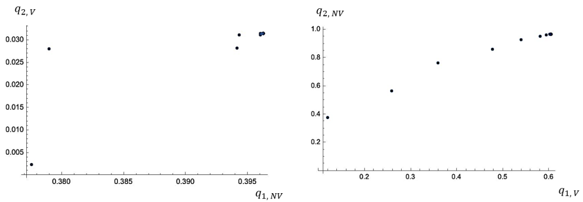
Figure 1: The convergence of lower bounds for each action

We discuss the general relationship between QRE and $\Delta^{p}$-rationalizable action distributions. Theorem 4.3 shows that every QRE is a $\Delta^{p}$-rationalizable, which is not surprising because, as mentioned above, each QRE is generated from a Bayesian equilibrium and it is a known result that that every Bayesian equilibrium satisfies rationality and common belief in rationality (See, for example, Battigalli et al. [6] and Chapter 8 of Battigalli et al. [4]). However, not every $\Delta^{p}$-rationalization procedure converges to a QRE as it does in the above example. Theorem 4.7 gives a sufficient condition for the convergence in $2\times 2$ games; further, the condition is necessary when there are multiple QREs. It is satisfied by many games that are intensively studied in the literature. Note that the condition only relies on the representative payoff functions but not on $p$. Generally, though the condition only provides a relaxed criterion, it is never satisfied except in some degenerate cases. Therefore, QRE may be too demanding as a prediction in general, and the infimum limits generated by the $\Delta^{p}$-rationalization procedure provide a robust benchmark to start from.

1.1 Two versions of QRE and their epistemic foundations

As mentioned in Footnote 1, there are two versions of QRE in the literature. The original one is given in MP, which is renamed as structural QRE (sQRE) in Goeree et al. [16]. MP generalizes McFadden [23]’s qualitative choice behavior model into quantal (i.e., discrete) choices into a game-theoretic framework for estimation using field and experimental data. Another version of QRE is introduced in McKelvey and Palfrey [25]. They use an axiomatic method to define quantal response functions, which describe players’ disturbed reactions to others’ mixed actions, and the equilibrium is a fixed-point in the system. It is renamed as regular QRE (rQRE) in Goeree et al. [16].

McKelvey and Palfrey [25] claimed that the two definitions are equivalent and structural QRE is the foundation of regular QRE. For a time, researches applied QRE without distinguishing the two (see Goeree et al. [16]). However, Haile et al. [19] (working paper in 2004) questioned the empirical content of QRE by showing that sQRE is not falsifiable in any static game. This forces researchers to distinguish the two QREs explicitly. One solution is provided by Goeree et al. [15], which redefined rQRE by putting additional restrictions on the quantal response functions and showed that some rQRE cannot be modeled as a sQRE and rQRE has empirical content.

From the decision-theoretical viewpoint, the two QREs correspond to the two models intended to interpret the phenomenon that in a population, the subjects’ responses over the set $A$ of alternatives under the same choice situation is governed by a probability mechanism $\pi$ (see Section 5 in Luce and Suppes [22] for a survey): sQRE corresponds to the random utility model where the utility function is selected according to some probability mechanism, while rQRE corresponds to the constant utility model where the utility function is fixed and the response probability is a function of it. The two models are based on different assumptions on each decision-maker’s rationality. The random utility model assumes that an individual’s behavior is optimal given her belief (i.e.,“rational”). In contrast, the constant utility model assumes bounded rationality (e.g., “trembling hands” in a sense similar to Selten [30]). This distinction is not emphasized sufficiently in the literature, which may lead to some conceptual concerns.

As an example, consider Goeree and Holt [14]’s noisy introspection (NI). Roughly speaking, NI is a hierarchical belief structure such that the higher the order is, the more random the response is supposed to be. NI is about rQRE, not sQRE. Because in the latter, the distribution of idiosyncrasies is commonly known (as implied in the definition given in MP) and has no reason to vary along the belief hierarchies. The increase of randomness can only be interpreted as due to individuals’ bounded rationality: For example, as the reasoning goes deeper, it is easier to make mistakes and harder to accurately predict others’ behavior. In this vein, our research studies only sQRE.

The rest of the paper is organized as follows. Section 2 provides preliminaries about QRE. Section 3 introduces $\Delta^{p}$-rationalization procedure and illustrates it with examples. Section 4 gives main results about the relationship between $\Delta^{p}$-rationalizability and QRE.

2 Quantal response equilibrium

Let $G=\langle I,(A_{j},u_{j})_{j\in I}\rangle$ be a static game, where $I$ is the finite set of players and for each $i\in I,A_{i}$ is the set of actions and $u_{i}:A$ $(:=\times_{j\in I}A_{j})\rightarrow\mathbb{R}$ is the von Neumann-Morgenstern payoff function of player $i$. Here, each player $i\in I$ is interpreted as a population with a representative payoff function $u_{i}$ and there is a random variable indicating individuals’ idiosyncrasies toward each action. Formally, we incorporate $G$ with a pair $\langle\Theta,p\rangle$ where $\Theta:=\times_{j\in I}\Theta_{j}$ and $p=(p_{j})_{j\in I}$ such that for each $i\in I$, $\Theta_{i}=\mathbb{R}^{A_{i}}$ and $p_{i}$ is a probability measure on $\Theta_{i}$ with a density function $f_{i}$ which has a marginal $f_{i,a_{i}}$ for each $a_{i}\in A_{i}$. For each $\pi=(\pi_{j})_{j\in I}\in\times_{j\in I}\Delta(A_{j})$, $i\in I$, and $a_{i}\in A_{i}$, we define

$$E_{i,a_{i}}(\pi)=\{\theta_{i}\in\Theta_{i}:u_{i}(a_{i},\pi_{-i})+\theta_{i,a_{i}}\geq u_{i}(a_{i}^{\prime},\pi_{-i})+\theta_{i,a_{i}^{\prime}}\text{ for each }a_{i}^{\prime}\in A_{i}\},$$

where $u_{i}(\cdot,\pi_{-i})$ is the expected value of $u_{i}(\cdot,a_{-i})$ with respect to $\pi_{-i}$. Here, $E_{i,a_{i}}(\pi)$ is the set of realizations of $\theta_{i}$ under which $a_{i}$ is a best response.

Definition 1.

Given $\langle G,\Theta,p\rangle$, a mixed action profile $\pi^{*}=(\pi_{j}^{*})_{j\in I}\in\times_{j\in I}\Delta(A_{j})$ is called a quantal response equilibrium (QRE) iff for each $i\in I$ and each $a_{i}\in A_{i}$, $\pi_{i}^{*}(a_{i})=p_{i}(E_{i,a_{i}}(\pi^{*}))$ .

3 $\Delta^{p}$-Rationalizability

3.1 Definitions

The strategic environment in Section 2 can be described as a game with payoff uncertainty (see, e.g., Battigalli et al. [4], Chapter 8)

$$\hat{G}=\langle I,(\Theta_{i},A_{i},U_{i})_{\in I}\rangle,$$

where for each $i\in I$, $\theta\in\Theta$, and $a\in A$, $U_{i}(\theta,a)=u_{i}(a)+\theta_{i,a_{i}}$. Each $\theta_{i}$ is called a payoff type (abbreviated as type in the following) of $i$. Since player $i$’s payoff is only influence by her own type $\theta_{i}$, the game has private values.

To simplify the symbols, with abuse of notations, in the following we use $\Delta(X\times Y)$ to denote the set of probability distributions on $X\times Y$ which have marginal distributions on both $X$ and $Y$. At the beginning of the game, an individual in population $i$ has a belief $\mu^{i}\in\Delta(\Theta_{-i}\times A_{-i})$ which does not vary across types in $\Theta_{i}$ and an individual in $i$ chooses a best response given her type. Since it is a game with private values, only her belief about the distributions of others’ actions, i.e., marg${}_{A_{-i}}\mu^{i}$, matters. Therefore, given a belief $\mu^{i}\in\Delta(\Theta_{-i}\times A_{-i})$, $a_{i}\in A_{i}$ is a best response to a belief $\mu^{i}$ under $\theta_{i}\in\Theta_{i}$ iff for each $a_{i}^{\prime}\in A_{i}$, $u_{i}(a_{i},\text{ marg}_{A_{-i}}\mu^{i})+\theta_{i,a_{i}}\geq u_{i}(a_{i}^{\prime},\text{ marg}_{A_{-i}}\mu^{i})+\theta_{i,a_{i}^{\prime}}$.

The distribution profile $p=(p_{i})_{i\in I}$ over $\Theta$ provides a ristriction on each individual’s first-order beliefs, that is, everyone’s marginal belief on each $\Theta_{j}$ should be coincide with $p_{j}$. Formally, we say that a belief $\mu^{i}\in\Delta(\Theta_{-i}\times A_{-i})$ of $i$ is consistent with $p$ iff

$$\mu^{i}=\prod_{j\neq i}\mu^{i}_{j}\text{ with }\mu_{j}^{i}\in\Delta(\Theta_{j}\times A_{j})\text{ and }\text{marg}_{\Theta_{j}}\mu^{i}_{j}=p_{j}\text{ for each }j\neq i$$ (1)

We use $\Delta^{p}_{i}$ to denote the set of all beliefs of $i$ satisfying (1).

The epistemic conditions are (EC1) Rationality, i.e., each individual in each population maximizes her expected utility based on her belief; (EC2) There is common belief in rationality; and (EC3) Transparency that everyone’s belief is consistent with the distribution $p$, i.e., everyone’s belief is consistent with $p$ and it is commonly believed so. The behavioral consequences of (EC1) - (EC3) are obtained by the iterative procedure defined as follows.

Definition 2.

Consider the following procedure, called $\Delta^{p}$-rationalization procedure:

Step 0. For each $i\in I$, $\Sigma_{i,\Delta^{p}}^{0}=\Theta_{i}\times A_{i}$,

Step $n+1$. For each $i=1,2$ and each $(\theta_{i},a_{i})\in\Theta_{i}\times A_{i}$ with $(\theta_{i},a_{i})\in\Sigma_{i,\Delta^{p}}^{n}$, $(\theta_{i},a_{i})\in\Sigma_{i,\Delta^{p}}^{n+1}$ iff the there is some $\mu^{i}\in\Delta^{p}_{i}$ such that

1. $a_{i}$ is a best response to $\mu^{i}$ under $\theta_{i}$, and

2. $\mu^{i}(\Sigma_{-i,\Delta^{p}}^{n})=1$ where $\Sigma_{-i,\Delta^{p}}^{n}:=\times_{j\neq i}\Sigma_{j,\Delta^{p}}^{n}$.

Let $\Sigma_{i,\Delta^{p}}^{\infty}=\cap_{n\geq 0}\Sigma_{i,\Delta^{p}}^{n}$ for $i\in I$. The elements in $\Sigma_{i,\Delta^{p}}^{\infty}$ are said to be $\Delta^{p}$-rationalizable.

Verbally, at each step, $(\theta_{i},a_{i})$ is eliminated if $a_{i}$ is not a best response under $\theta_{i}$ to any belief consistent with $p$ whose support is those $(\theta_{-i},a_{-i})$ surviving until the previous step. Since it is a special case of $\Delta$-rationalizability in Battigalli and Siniscalchi [8] which is restricted by $p$, we call it $\Delta^{p}$-rationalizability. Here we focus on $\Delta^{p}$-rationalizable action distributions, i.e., the action distributions obtained from $p$ and $\Delta^{p}$-rationalizable outcomes.

Definition 3.

We call $\pi_{i}\in\Delta(A_{i})$ an $n$th-order $\Delta^{p}$-rationalizable action distribution for $i$ iff there is $\mu_{i}\in\Delta(\Theta_{i}\times A_{i})$ with $\mu_{i}(\Sigma_{i,\Delta^{p}}^{n})=1$ and marg${}_{\Theta_{i}}\mu_{i}=p_{i}$ such that $\pi_{i}=$ marg${}_{A_{i}}\mu_{i}$. We call $\pi_{i}$ $\Delta^{p}$-rationalizable iff it is $n$th-order $\Delta^{p}$-rationalizable for each $n\in\mathbb{N}$.

For example, for each $i\in I$, consider a pushforward function $\sigma_{i}:\Theta_{i}\rightarrow A_{i}$ such that for each $\theta_{i}\in\Theta_{i}$, $(\theta_{i},\sigma_{i}(\theta_{i}))\in\Sigma_{i,\Delta^{p}}^{\infty}$ (or in $\Sigma_{i,\Delta^{p}}^{n}$ for some $n\in\mathbb{N}$). Define $\pi_{i}\in\Delta(A_{i})$ such that $\pi_{i}(a_{i})=p_{i}(\sigma_{i}^{-1}(a_{i}))$. It is clear that $\pi_{i}$ is ($n$-th order) $\Delta^{p}$-rationalizable.

3.2 Examples

Example 3.1.

Consider the game in Table 2 and $p=p_{1}\times p_{2}$ where each $p_{i}(i=1,2)$ is the uniform distribution on $[-2,2]\times[-2,2]$. The unique QRE of this game is $\pi^{*}=(1/2H+1/2T,1/2H+1/2T)$. We show that, for each $i=1,2$, the only $\Delta^{p}$-rationalizable distribution is $\pi^{*}_{i}$.

$1\setminus 2$	$H$	$T$
$H$	$1,0$	$0,1$
$T$	$0,1$	$1,0$

Table 2: Example 3.1

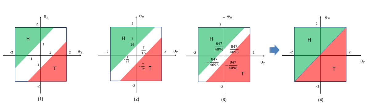
Figure 2: The $\Delta^{p}$-rationalization procedure converges to the QRE

First, let $i\in I$ and $\theta_{i}=(\theta_{iH},\theta_{iT})\in\Theta_{i}$. Then $(\theta_{i},H)\in\Sigma_{i,\Delta^{p}}^{1}$ if and only if for some $qH+(1-q)T\in\Delta(A_{-i})$, $q+\theta_{iH}\geq(1-q)+\theta_{iT}$, or, equivalently,

$$\theta_{iH}-\theta_{iT}\geq 1-2q$$ (2)

Since $q\in[0,1]$, when $\theta_{iH}-\theta_{iT}\geq 1-2\times 0=1$ (the green area in Figure 2 (1)), $(\theta_{i},H)\in\Sigma_{i,\Delta^{p}}^{1}$. Similarly, when $\theta_{iT}-\theta_{iH}\geq 1$ (the red area in Figure 2 (1)), $(\theta_{i},T)\in\Sigma_{i,\Delta^{p}}^{1}$. To every type between them (i.e., the white area) both $H$ and $T$ can be associated.

Therefore, the measures of the green (red) area provides the infimums of the probabilities that $H$ ($T$) in the beliefs at the second step in the procedure. Note that the probability measure of each area is $\frac{9}{32}$. It means that to satisfy $\mu^{i}\in\Delta^{p}_{i}$ and $\mu^{i}(\Sigma_{-i,\Delta^{p}}^{1})=1$, both marg${}_{A_{-i}}\mu^{i}(H)$ and marg${}_{A_{-i}}\mu^{i}(T)$ are at least $\frac{9}{32}$. Under this new restriction, inequality (2) implies that when $\theta_{iH}-\theta_{iT}\geq 1-2\times\frac{9}{32}=\frac{7}{16}$, $(\theta_{i},H)\in\Sigma_{i,\Delta^{p}}^{2}$. Similarly, when $\theta_{iT}-\theta_{iH}\geq\frac{7}{16}$, $(\theta_{i},T)\in\Sigma_{i,\Delta^{p}}^{2}$. Those areas are the green and red ones in Figure 2 (2), respectively. Now we obtain restrictions on for the beliefs in the second step of the $\Delta^{p}$-rationalization procedure, which is shown in Figure 2 (3).

In generally, let $q^{n}_{i,a_{i}}$ be the infimum of the probability of using $a_{i}\in\{H,T\}$ in beliefs at step $n$. Then $q^{0}_{i,a_{i}}=0$ and for $n\geq 0$,

$$q^{n+1}_{i,a_{i}}=\frac{(3+2q^{n}_{i,a_{i}})^{2}}{32},$$

which is bounded and increasing; hence $\lim_{n\rightarrow\infty}q^{n}_{i,a_{i}}=1/2$, i.e., the QRE distribution. $\blacktriangle$

Example 3.2.

Consider an asymmetric Matching-Pennies game in Table 3. Here, $p=\prod_{i=1,2;k=H,T}p_{ik}$ where each $p_{ik}$ is the extreme value distribution with $\lambda=5$. This game has only one QRE (Goeree et al. [16], Chapter 2.2).

$1\setminus 2$	$H$	$T$
$H$	$9,0$	$0,1$
$T$	$0,1$	$1,0$

Table 3: Example 3.2

It can be shown that for each $i=1,2,a_{i}=H,T$, the infimum sequence $(q_{i,a_{i}}^{n})_{n=0}^{\infty}$ converges to some number extremely close to $0$, which is not a QRE since the sum of each pair is strictly less than 1. $\blacktriangle$

4 QRE and $\Delta^{p}$-rationalizability

4.1 QRE $\rightarrow\Delta^{p}$-rationalizability

Our first result is that every QRE is $\Delta^{p}$-rationalizable. This is the counterpart of the classic result that each Nash equilibrium action is rationalizable (Bernheim [10], Pearce [28]).

Theorem 4.3.

Consider a static game $G=\langle I,(A_{j},u_{j})_{j\in I}\rangle$ and $\langle\Theta,p\rangle$ and let $\pi=(\pi_{j})_{j\in I}$ be a QRE. For each $i\in I$, $\pi_{i}$ is $\Delta^{p}$-rationalizable.

Proof 4.4.

Fix $i\in I$. We have to construct a $\mu_{i}\in\Delta(\Theta_{i}\times A_{i})$ with $\mu_{i}(\Sigma_{i,\Delta^{p}}^{n})=1$ for each $n\in\mathbb{N}$ and marg${}_{\Theta_{i}}\mu_{i}=p_{i}$ such that $\pi_{i}=$ marg${}_{A_{i}}\mu_{i}$.

For each $j\in I$, let $<_{j}$ be an asymmetric linear order on $A_{j}$; hence for each non-empty $A_{j}^{\prime}\subseteq A_{j}$, $\max A_{j}^{\prime}$ is well defined. Recall that for each $a_{j}\in A_{j}$, $E_{j,a_{j}}(\pi)$ is the set of $\theta_{j}$’s under which $a_{j}$ is a best response to $\pi_{-j}$. Now for each $\theta_{j}\in\Theta_{j}$, we define $A_{j,\theta_{j}}(\pi)=\{a_{j}\in A_{j}:\theta_{j}\in E_{j,a_{j}}(\pi)\}$, i.e., the set of best responses of $j$ against $\pi_{-j}$ under $\theta_{j}$. It is clear that $A_{j,\theta_{j}}(\pi)\neq\emptyset$ for each $\theta_{j}$. Define a mapping $c_{j}:\Theta_{j}\rightarrow A_{j}$ such that $c_{j}(\theta_{j})=\max A_{j,\theta_{j}}(\pi)$. Note that for a “boundary” $\theta_{j}$, i.e., $|A_{j,\theta_{j}}(\pi)|>1$, $c_{j}(\theta_{j})$ is just a tie breaker; this does not cause any problem since $\pi_{j}$ is a probability distribution and those “boundary” payoff types form a null set with respect to $p_{j}$.

It can be seen that $c_{j}$ is measurable, because for each $a_{j}\in A_{j}$, $c_{j}^{-1}(a_{j})$ is either $E_{j,a_{j}}$ or $E_{j,a_{j}}\setminus\cap_{a_{j}^{\prime}\in A_{j}^{\prime}}E_{j,a_{j}^{\prime}}$ for some $A_{j}^{\prime}\subseteq A_{j}$, both measurable. Let Gr$(c_{j})=\{(\theta_{j},c_{j}(\theta_{j}):\theta_{j}\in\Theta_{j}\}$, i.e., the graph of $c_{j}$. Now we define $\mu_{j}\in\Delta(\Theta_{j}\times A_{j})$. For each $X\subseteq\Theta_{j}\times A_{j}$, we say $X$ is measurable iff $proj_{\Theta_{j}}[X\cap$ Gr$(c_{j})]$ is measurable in $\Theta_{j}$. For each measurable $X$, define $\mu_{j}(X)=p_{j}(proj_{\Theta_{j}}[X\cap$ Gr$(c_{j})])$. It is straightforward to see that marg${}_{\Theta_{j}}\mu_{j}=p_{j}$ and for each $a_{j}\in A_{j}$, marg${}_{A_{j}}\mu_{j}(a_{j})=p_{j}[E_{j,a_{j}}(\pi)]=\pi_{j}(a_{j})$.

Let $\mu^{i}=\prod_{j\neq i}\mu_{j}$. Since $\pi$ is a QRE, it is clear that under each $\theta_{i}$, $c_{i}(\theta_{i})$ is a best response to $\mu^{i}$. This fixed-point property guarantees that $(\theta_{i},c_{i})\in\Sigma_{i,\Delta^{p}}^{n}$ for each $n\in\mathbb{N}$. Therefore, $\pi_{i}=$ marg${}_{A_{i}}\mu_{i}$ is $\Delta^{p}$-rationalizable.

4.2 $\Delta^{p}$-rationalizability $\rightarrow$ QRE

Examples in Section 3.2 suggest that the converse of Theorem 4.3 is not true in general. Our concern is when it is true, that is, when QRE distributions provide a “tight" prediction of the behavioral consequence when we assume rationality, common belief in rationality, and transparency that individuals’ beliefs are consistent with the distribution p of the idiosyncrasies.

Consider a static game $G=\langle I,(A_{i},u_{i})_{i\in I}\rangle$ with $\langle\Theta,p\rangle$. We use $Q(G,\Theta,p)$ to denote the set of QREs. Brouwer’s fixed point theorem guarantees that here $Q(G,\Theta,p)\neq\emptyset$. For each $i\in I$ and $a_{i}\in A_{i}$, we define

$$\underline{\pi}_{i,a_{i}}=\inf\{\pi_{i}(a_{i}):(\pi_{i},\pi_{-i})\in Q(G,\Theta,p)\text{ for some }\pi_{-i}\in\Delta{A_{-i}}\},$$ (3)

and for each $n\in\mathbb{N}$, we define

$$q_{i,a_{i}}^{n}=\inf\{\pi_{i}(a_{i}):\pi_{i}\text{ is }n\text{-th order }\Delta^{p}\text{-rationalizable}\}$$ (4)

We first show that for each $i\in I$ and $a_{i}\in A_{i}$, $(q_{i,a_{i}}^{n})_{n\in\mathbb{N}}$ converges to some $q_{i,a_{i}}^{*}\leq\underline{\pi}_{i,a_{i}}$ (Proposition 4.5). Then we gives a sufficient condition on $2\times 2$ games under which $q_{i,a_{i}}^{*}$ is the probability that action $a_{i}$ is used in some QRE; when $|Q(G,\Theta,p)|>1$, the condition is necessary (Theorem 4.7). We will also discuss how strict the condition is in general.

Proposition 4.5.

For each $i\in I$ and $a_{i}\in A_{i}$, the sequence $(q_{i,a_{i}}^{n})_{n\in\mathbb{N}}$ is bounded and non-decreasing. Hence, there is some $q_{i,a_{i}}^{*}$ such that $\lim_{n\rightarrow\infty}q_{i,a_{i}}^{n}=q_{i,a_{i}}^{*}$. In addition, $q_{i,a_{i}}^{*}\leq\underline{\pi}_{i,a_{i}}$.

Proof 4.6.

Fix $i\in I$ and $a_{i}\in A_{i}$. First, it is clear that for each $j\in I$ and $a_{j}\in A_{j}$, $p_{j,a_{j}}^{0}=0$. Consider step $n\geq 0$ in the $\Delta^{p}$-rationalization procedure. Suppose that each $(q_{j,a_{j}}^{k})_{k=0}^{n}$ is non-decreasing. At step $n+1$, $q_{i,a_{i}}^{n+1}$ is determined by the set of $\theta_{i}\in\Theta_{i}$ for which only $(\theta_{i},a_{i})$ is $\Delta^{p}$-rationalizable, i.e., the set of $\theta_{i}$ such that for each $a_{i}^{\prime}\in A_{i}$ and each $n$-th $\Delta^{p}$-rationalizable $q_{-i}$,

$$\theta_{i,a_{i}}-\theta_{i,a_{i}^{\prime}}\geq\sum_{a_{-i}\in A_{-i}}q_{-i}(a_{-i})[u_{i}(a_{i}^{\prime},a_{-i})-u_{i}(a_{i},a_{-i})]$$ (5)

The feasible region is determined by $q_{j,a_{j}}^{n}\leq q_{j}(a_{j}\leq 1$ ($a_{j})\in A_{j}$) and $\sum_{a_{j}^{\prime}}q_{j}(a_{j}^{\prime})=1$. By inductive assumption, $q_{j,a_{j}}^{n-1}\leq q_{j,a_{j}}^{n}$ for each $j\neq i$ and $a_{j}\in A_{j}$. Hence the feasible region shrinks, which implies that $q_{i,a_{i}}^{n}\leq q_{i,a_{i}}^{n+1}$. Since $(q_{i,a_{i}}^{n})_{n\in\mathbb{N}}$ is non-decreasing and bounded within $[0,1]$, it converges to some $q_{i,a_{i}}^{*}$. Since Theorem 4.3 shows that $\underline{\pi}_{i,a_{i}}$ is $\Delta^{p}$-rationalizable, it follows that $q_{i,a_{i}}^{*}\leq\underline{\pi}_{i,a_{i}}$.

We now study when the converse of Theorem 4.3 holds, or, equivalently, under what conditions, $q_{i,a_{i}}^{*}$ is the probability that $a_{i}$ is used in some QRE for $i\in I$ and $a_{i}\in A_{i}$.

Consider a 2-person game $G=\langle A_{1},A_{2},u_{1},u_{2}\rangle$. For each $i\in I$ and $a_{i},a_{i}^{\prime}\in A_{i}$, we let $\overline{H}_{i}^{a_{i},a_{i}^{\prime}}=\max_{a_{-i}\in A_{-i}}(u_{i}(a_{i}^{\prime},a_{-i})-u_{i}(a_{i},a_{-i}))$ and $\underline{H}_{i}^{a_{i},a_{i}^{\prime}}=\min_{a_{-i}\in A_{-i}}(u_{i}(a_{i}^{\prime},a_{-i})-u_{i}(a_{i},a_{-i}))$. It is easy to see that $\overline{H}_{i}^{a_{i}^{\prime},a_{i}}=-\underline{H}_{i}^{a_{i},a_{i}^{\prime}}$, i.e., $\underline{H}_{i}^{a_{i}^{\prime},a_{i}}=-\overline{H}_{i}^{a_{i},a_{i}^{\prime}}$.

Based on this, we define $\phi_{i}:A_{i}\times A_{i}\rightarrow 2^{A_{-i}}$ such that for each $(a_{i},a_{i}^{\prime})\in A_{i}\times A_{i}$, $\phi_{i}(a_{i},a_{i}^{\prime})=\{a_{-i}\in A_{-i}:u_{i}(a_{i}^{\prime},a_{-i})-u_{i}(a_{i},a_{-i})<\overline{H}_{i}^{a_{i},a_{i}^{\prime}}\}$. Based on $\phi_{i}$, we define a correspondence $\Phi_{i}:A_{i}\rightarrow 2^{A_{-i}}$ such that $\Phi_{i}(a_{i})=\cup_{a_{i}^{\prime}}\phi_{i}(a_{i},a_{i}^{\prime})$ for each $i\in I$ and $a_{i}\in A_{i}$. Each $a_{-i}\in\Phi_{i}(a_{i})$ is called a marginal actions for $a_{i}$ since the infimums of the probabilities that those actions are used determines the area in $\Theta_{i}$ where $a_{i}$ is solely favored. An action $a_{i}\in A_{i}$ is called non-serial iff $\Phi(a_{i})=\emptyset$; it is called eventually non-serial iff for some $a_{-i}\in\Phi(a_{i})$, $\Phi(a_{-i})=\emptyset$. A game serial iff no action is non-serial.

We can visualize $(\Phi_{1},\Phi_{2})$ by a directed graph $(\Rightarrow,A_{1}\cup A_{2})$ such that for each $a_{i},a_{j}\in A_{1}\cup A_{2}$, $a_{i}\Rightarrow a_{j}$ iff $a_{j}\in\Phi_{i}(a_{i})$. For example, Figure 3 (1) is thegraph of the game in Table 1 and Figure 3 (2) is that of Example 3.2. Theorem 4.7 will show that a generic game with a graph like the former has $\lim_{n\rightarrow\infty}q_{i,a_{i}}^{n}=\underline{\pi}_{i,a_{i}}$, and when the game has multiple QREs, the conditions are both necessary and sufficient.

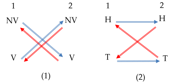
Figure 3: The graphs for two games

Theorem 4.7.

Consider a $2\times 2$ game and $a_{i}\in A_{i}$ for some $i\in I$. If one of the following conditions is satisfied, then $q_{i,a_{i}}^{*}=\underline{\pi}_{i,a_{i}}$:

C1 $a_{i}$ is eventually non-serial, or

C2 $|\Phi_{i}(a_{i})|=1$ and $\Phi_{-i}(\Phi_{i}(a_{i}))=\{a_{i}\}$.

Further, if $|Q(G,\Theta,p)|>1$ and both C1 and C2 are violated for one action, $q_{i,a_{i}}^{*}<\underline{\pi}_{i,a_{i}}$ for each $i\in I$ and $a_{i}\in A_{i}$.

Before showing Theorem 4.7, we need some lemma.

Lemma 4.8.

Consider $i\in\{1,2\}$ and distinct $a_{i},a_{i}^{\prime}\in A_{i}$. Either $\phi_{i}(a_{i},a_{i}^{\prime})=\phi_{i}(a_{i}^{\prime},a_{i})=\emptyset$ or $\phi_{i}(a_{i},a_{i}^{\prime})\cup\phi_{i}(a_{i}^{\prime},a_{i})=A_{-i}$.

Proof 4.9.

If $\phi_{i}(a_{i},a_{i}^{\prime})=\emptyset$, then $u_{i}(a_{i}^{\prime},a_{-i})-u_{i}(a_{i},a_{-i})=\overline{H}_{i}^{a_{i},a_{i}^{\prime}}$ for each $a_{-i}\in A_{-i}$, which implies that $u_{i}(a_{i},a_{-i})-u_{i}(a_{i}^{\prime},a_{-i})$ is constant on $A_{-i}$, i.e., $\phi_{i}(a_{i}^{\prime},a_{i})=\emptyset$. Suppose that $\phi_{i}(a_{i},a_{i}^{\prime})\neq\emptyset$, which implies that $\overline{H}_{i}^{a_{i},a_{i}^{\prime}}>\underline{H}_{i}^{a_{i},a_{i}^{\prime}}$. Since $u_{i}(a_{i},a_{-i})-u_{i}(a_{i}^{\prime},a_{-i})=-(u_{i}(a_{i}^{\prime},a_{-i})-u_{i}(a_{i},a_{-i}))$, it follows that $(A_{-i}\setminus\phi_{i}(a_{i},a_{i}^{\prime}))\subseteq\phi_{i}(a_{i}^{\prime},a_{i})$, and consequently $\phi_{i}(a_{i},a_{i}^{\prime})\cup\phi_{i}(a_{i}^{\prime},a_{i})=A_{-i}$.

Proof 4.10 (Proof of Theorem 4.7).

First, suppose that $a_{i}$ is non-serial, i.e., $u_{i}(a_{i}^{\prime},a_{-i})-u_{i}(a_{i},a_{-i})=\overline{H}_{i}^{a_{i},a_{i}^{\prime}}$ for each $a_{-i}\in A_{-i}$ ($a_{i}^{\prime}\neq a_{i}$). For each $n\geq 0$, define $E_{i,a_{i}}^{n+1}$ to be set set of all $\theta_{i}\in\Theta_{i}$ satisfying

$$\theta_{i,a_{i}}-\theta_{i,a_{i}^{\prime}}\geq\max_{q_{-i}\text{ is }n\text{-th }\Delta^{p}\text{-rationalizable}}\sum_{a_{-i}\in A_{-i}}q_{-i}(a_{-i})[u_{i}(a_{i}^{\prime},a_{-i})-u_{i}(a_{i},a_{-i})]$$ (6)

It follows that here, $E_{i,a_{i}}^{n+1}=E_{i,a_{i}}^{1}$ $=\{\theta_{i}:\theta_{i,a_{i}}-\theta_{i,a_{i}^{\prime}}\geq\overline{H}_{i}^{a_{i},a_{i}^{\prime}}\}$ for each $n\geq 0$, and consequently $q_{i,a_{i}}^{*}=p_{i}(E^{1}_{i,a_{i}})$. Further, since for each $q\in\Delta(A_{1})\times\Delta(A_{2})$, $E_{i,a_{i}}(q)=E_{i,a_{i}}^{1}$, hence $q_{i,a_{i}}^{*}=p_{i}(E_{i,a_{i}}(q))$, By Proposition 4.5, $q_{i,a_{i}}^{*}=\underline{\pi}_{i,a_{i}}$. Similarly, if $a_{i}$ is eventually non-serial, since the probabilities of their marginal actions will be fixed from the first round, $E_{i,a_{i}}^{n}=E_{i,a_{i}}^{2}$ for each $n\geq 2$, and we still have $q_{i,a_{i}}^{*}=\underline{\pi}_{i,a_{i}}$.

Now suppose that $a_{i}$ satisfies C2 with $a_{j}$ be the unique element in $\Theta_{i}(a_{i})$ ($j\neq i$). Let $A_{i}=\{a_{i},a_{i}^{\prime}\}$ and $A_{j}=\{a_{j},a_{j}^{\prime}\}$. Lemma 4.8 implies that $\Phi_{i}(a_{i}^{\prime})=a_{j}^{\prime}$ and $\Phi_{j}(a_{j}^{\prime})=a_{i}^{\prime}$. We show that the following $q$ is a QRE:

$$q_{i}(a_{i})=q_{i,a_{i}}^{*},q_{i}(a_{i}^{\prime})=1-q_{i,a_{i}}^{*},q_{j}(a_{j})=q_{j,a_{j}}^{*},q_{i}(a_{i}^{\prime})=1-q_{j,a_{j}}^{*}$$

First, at the limit,

$$q_{i,a_{i}}^{*}=p_{i}(\{\theta_{i}\in\Theta_{i}:\theta_{i,a_{i}}-\theta_{i,a_{i}^{\prime}}\geq(1-q_{j,a_{j}}^{*})\overline{H}_{1}^{a_{i},a_{i}^{\prime}}+q_{j,a_{j}}^{*}\underline{H}_{i}^{a_{i},a_{i}^{\prime}}\})$$ (7)

Hence, if $q^{*}_{i,a_{i}}$ is the probability that $i$ uses $a_{i}$ in some QRE, it requires that $j$ uses $a_{j}$ with $q_{j,a_{j}}^{*}$. Since at the limit,

$$q_{j,a_{j}}^{*}=p_{j}(\{\theta_{j}\in\Theta_{j}:\theta_{j,a_{j}}-\theta_{j,a_{j}^{\prime}}\leq q_{i,a_{i}}^{*}\overline{H}_{j}^{a_{j},a_{j}^{\prime}}+(1-q_{i,a_{i}}^{*})\underline{H}_{j}^{a_{j},a_{j}^{\prime}}\}).$$ (8)

Hence $q_{i,a_{i}}^{*}$ and $q_{j,a_{j}}^{*}$ are mutually fulfilling. In addition, when $q_{j}(a_{j}^{\prime})=1-q_{j,a_{j}}^{*}$, each $\theta_{1}\in\Theta_{i}\setminus\{\theta_{i}\in\Theta_{i}:\theta_{i,a_{i}}-\theta_{i,a_{i}^{\prime}}\geq(1-q_{j,a_{j}}^{*})\overline{H}_{1}^{a_{i},a_{i}^{\prime}}+q_{j,a_{j}}^{*}\underline{H}_{i}^{a_{i},a_{i}^{\prime}}\}$ $=\{\theta_{i}\in\Theta_{i}:\theta_{i,a_{i}^{\prime}}-\theta_{i,a_{i}}>(1-q_{j,a_{j}}^{*})(u_{i}(a_{i},a_{j}^{\prime})-u_{i}(a_{i}^{\prime},a_{j}^{\prime}))+q_{j,a_{j}}^{*}(u_{i}(a_{i},a_{j})-u_{i}(a_{i}^{\prime},a_{j}))\}$ and the measure of the latter set is $1-q_{i,a_{i}}^{*}$, i.e., $p_{i}(E_{i,a_{i}^{\prime}})$. The same calculation works for $a_{j}^{\prime}$. Hence, $q$ is a QRE.

Suppose that $|Q(G,\Theta,p)|>1$ and both C1 and C2 are violated for one action. It follows that for distinct $\pi,\pi^{\prime}\in Q(G,\Theta,p)$, each $j\in I$ and $a_{j}\in A_{j}$, $\pi_{j}(a_{j})\neq\pi_{j}^{\prime}(a_{j})$. Therefore, $\sum_{a_{j}^{\prime}\in A_{j}}\underline{\pi}_{j,a_{j}}<1$ for each $j\in I$. Suppose that $q_{i,a_{i}}^{*}=\underline{\pi}_{i,a_{i}}$ for some $i\in I$ and $a_{i}\in A_{i}$. Since now every pair oin $A_{1}\cup A_{2}$ are reachable from the other, if $a_{i}$ is used in some QRE by probability $q_{i,a_{i}}^{*}$, it requires each action $a_{j}$ is used by probability $q_{j,a_{j}}^{*}$, which does not form a probability distribution. Hence $q_{i,a_{i}}^{*}<\underline{\pi}_{i,a_{i}}$ for each $i\in I$ and $a_{i}\in A_{i}$.

Note that C1 and C2 relies only on $G$ but not on $\langle\Theta,p\rangle$. Hence the convergence is not influenced by changing $\langle\Theta,p\rangle$ (e.g., changing the parameters in the distribution class) even though the latter may change the QRE. C1 means the payoff matrix of player $i$ has order 1, which is quite restrictive. C2 is more general and many games intensively studied in the literature satisfy C2, for example, the asymmetric chicken game (Goeree et al. [16], p.25-26), coordination games (Goeree et al. [16], p.29-30, Anderson et al. [2], Turocy [32]), and many (but not all) dominance-solvable games. However, a Matching-Pennies style game (MP, Ochs [27]) never satisfies C2. A direct implication of Theorem 4.7 is that when $|Q(G,\Theta,p)|=1$ and either C1 or C2 in Theorem 4.7 is satisfied, the QRE is the only $\Delta^{p}$-rationalizable action distribution. Hence Theorem 4.7 provide a sufficient conditions for using QRE as the robust and tight prediction about the population behavior when the epistemic conditions are satisfied.

4.2.1 The strictness of the conditions and a full convergence

Conditions in Theorem 4.7 could also be well-defined on general $n$-person games. Yet there they could only provide relaxed criteria instead of a sufficient condition. One may wonder how ‘large” the set of games satisfying them could be. We have the following result.

Proposition 4.11.

Consider a 2-person serial game with $|A_{i}|\geq 2$ for each $i=1,2$ and at least one player has more than two actions. Then no action satisfies condition (2) in Theorem 2.

Proof 4.12.

Without loss of generality, suppose that $|A_{1}|>2$ and $a_{1}\in A_{1}$ satisfies C2. Suppose that $\Phi_{1}(a_{1})=\{a_{2}\}$ for some $a_{2}\in A_{2}$ and $R(a_{1})=\{a_{1},a_{2}\}$. Let $b_{1},c_{1}\in A_{1}\setminus\{a_{1}\}$ be distinct. By Lemma 4.8, $\Phi_{1}(b_{1})\cup\Phi_{1}(c_{1})=A_{2}$. So $a_{2}\in\Phi_{1}(b_{1})$ or $a_{2}\in\Phi_{1}(c_{1})$, violating C2.

Proposition 4.11 implies that C2 in Theorem 4.7 cannot be satisfied in a generic $n$-person game ($n>2$). Even if each player has only two actions, since $\Phi_{i}(a_{i})$ now contains profiles of actions in $A_{-i}=\prod_{j\neq i}A_{j}$ and $|A_{-i}|>2$, through an argument similar to the proof of Proposition 4.11, it can be seen that no action satisfies C2 in Theorem 2. Therefore, in general, QRE is a proper subset of the $\Delta^{p}$-rationalizable action distributions.

Remark 4.13.

One may wonder whether C2 can be relaxed in general 2-person games. The proof of Theorem 4.7 suggests that whether we can build a QRE where the probability of choosing $a$ is $q_{i,a_{i}}^{*}$ depends on whether the set of all actions which are directly or indirectly influenced by or influences $a_{i}$, denoted by $R(a_{i})$, coincides with $A_{1}\cup A_{2}$; if the answer is no, then $q_{i,a_{i}}^{*}=\underline{\pi}_{i,a_{i}}$. This may suggest us to replace C2 by a more general condition C2’: $R(a_{i})\neq A_{1}\cup A_{2}$. However, from Lemma 4.8 one can prove that (C2) and (C2’) are equivalent. Hence C2 is not as strict as it looks like in more general cases.

References

- [1] Alaoui L, Penta A (2016) Endogenous depth of reasoning. The Review of Economic Studies 83: 1297-1333.
- [2] Anderson, SP, Goeree JK, Holt CA (2001) Minimum-effect coordination games: stochastic potential and logit equilibrium. Games and Economic Behavior 34: 174-199.
- [3] Aumann R, Brandenburger A (1995) Epistemic conditions for Nash equilibrium. Econometrica 63: 1161-1180.
- [4] Battigalli P, Catonini E, De Vito N (2022) Game Theory: Analysis of Strategic Thinking. Lecture notes.
- [5] Battigalli P, Catinini E (2023) The epistemic spirit of divinity. Working paper.
- [6] Battigalli P, Freidenberg A, Siniscalchi M (2020) Epistemic Game Theory: Reasoning About Strategic Uncertainty. Manuscript.
- [7] Battigalli P, Prestipino A (2013) Transparent restrictions on beliefs and forward-Induction reasoning in games with asymmetric information. The B.E. Journal of Theoretical Economics 13: 79-130.
- [8] Battigalli P, Siniscalchi M (2003) Rationalization and incomplete information. Advances in Theoretical Economics 3, Article 3.
- [9] Bergemann D, Morris S (2005) Robust mechanism design. Econometrica 73: 1771-1813.
- [10] Bernheim BD (1984) Rationalizable strategic behavior. Econometrica 52: 1007-1028.
- [11] Blackburn P, De Rijke M, Venema Y (2001). Modal logic. Cambridge University Press.
- [12] Dekel E, Siniscalchi M (2015) Epistemic game theory. In: Young PH, Zamir S (eds) Handbooks of game theory with economic applications, vol 4. Elsevier, Amsterdam, pp 619–702
- [13] Friedenberg A, Kets W, Kneeland T (2021) Is bounded reasoning about rationality driven by limited ability? Working paper.
- [14] Goeree JK, Holt CA (2004) A model of noisy introspection. Games and Economic Behavior 46: 365-382.
- [15] Goeree JK, Holt CA, Palfrey TR. 2005. Regular quantal response equilibrium. Experimental Economics 8: 347-367.
- [16] Goeree JK, Holt CA, Palfrey TR (2016) Quantal Response Equilibrium. Princeton University Press.
- [17] Harsanyi J (1967-68) Games of incomplete information played by Bayesian players, Parts I-III. Management Science 14: 159-182, 320-334, 486-502.
- [18] Harsanyi J (1973) Games with randomly disturbed payoffs: a new rationale for mixed-strategy equilibrium points. International Journal of Game Theory 2: 1-23.
- [19] Haile PA, Hortaçsu A, Kosenok G. 2008. On the empirical content of quantal response equilibrium. American Economic Review 98: 180-200.
- [20] Kneeland T (2015) Identyfying higher-order rationality. Econometrica 83: 2065-2079.
- [21] Kneeland T (2016) Coordination under limited depth of reasoning. Games and Economic Behavior 96: 49-64.
- [22] Luce R, Suppes P (1965) Preference, utility, and subjective probability. In Handbook of Mathematical Psychology, vol 3, ed. by Luce R, Bush R, and Galanter E. Wiley.
- [23] McFadden D (1973) Conditional logit analysis of qualitative choice behavior. In Frontiers of Econometrics, P. Zarembka ed. Academic Press, New York.
- [24] McKelvey RD, Palfrey TR (1995) Quantal response equilibria for normal form games. Games and Economic Behavior 10: 6-38.
- [25] McKelvey RD, Palfrey TR (1996) A statistical theory of equilibrium in games. Japanese Economic Review 47: 186-209.
- [26] Melo E (2021) On the uniqueness of quantal response equilibria and its application to network games. Working paper.
- [27] Ochs J (1995) Games with unique mixed strategy equilibria: an experimental study. Games and Economic Behavior 10: 174-189.
- [28] Pearce D (1984) Rationalizable strategic behavior and the problem of perfection. Econometrica 52: 1029-1050.
- [29] Polak B (1999) Epistemic conditions for Nash equilibrium, and common knowledge of rationality. Econometrica 67: 673-676.
- [30] Selten R (1975) A reexamination of the perfectness concept for equilibrium points in extensive games. International Journal of Game Theory 4: 25-55.
- [31] Tan T, Werlang SRC (1988) The Bayesian foundation of solution concepts of games. Journal of Economic Theory 45: 370-391.
- [32] Turocy TL (2005) A dynamic homotopy interpretation of the logistic quantal response equilibrium correspondence. Games and Economic Behavior 51: 242-263.
- [33] Weinstein J, Yildiz M (2007) A Structure Theorem for Rationalizability with Application to Robust Predictions of Refinements. Econometrica 75: 365–400.