On simultaneous linearization of certain commuting nearly integrable diffeomorphisms of the cylinder

Abstract.

Let $\mathcal{F}$ and $\mathcal{K}$ be commuting $C^{\infty}$ diffeomorphisms of the cylinder $\mathbb{T}\times\mathbb{R}$ that are, respectively, close to $\mathcal{F}_{0}(x,y)=(x+\omega(y),y)$ and $T_{\alpha}(x,y)=(x+\alpha,y)$, where $\omega(y)$ is non-degenerate and $\alpha$ is Diophantine. Using the KAM iterative scheme for the group action we show that $\mathcal{F}$ and $\mathcal{K}$ are simultaneously $C^{\infty}$-linearizable if $\mathcal{F}$ has the intersection property (including the exact symplectic maps) and $\mathcal{K}$ satisfies a semi-conjugacy condition. We also provide examples showing necessity of these conditions. As a consequence, we get local rigidity of certain class of $\mathbb{Z}^{2}$-actions on the cylinder, generated by commuting twist maps.

1. Introduction

The goal of this paper is to study the simultaneous linearization problem for some commuting nearly integrable $C^{\infty}$ diffeomorphisms of the cylinder. The question of linearization has been one of the central themes in dynamical systems. We start by considering two types of typical integrable maps on the infinite cylinder $\mathbb{T}\times\mathbb{R}$, whose perturbations will be discussed below. Here, $\mathbb{T}=\mathbb{R}/\mathbb{Z}$ denotes the circle. Let $\mathcal{F}_{0}:\mathbb{T}\times\mathbb{R}\to\mathbb{T}\times\mathbb{R}$ be a smooth integrable twist map of the form

$$\mathcal{F}_{0}(x,y)=(x+\omega(y),y),$$

where the frequency map $\omega(y)$ is non-degenerate, in the sense that $\omega(y):\mathbb{R}\to\mathbb{R}$ has a smooth inverse map. A typical example is $\omega(y)=y$. For $\alpha\in\mathbb{R}$, we denote by $T_{\alpha}:\mathbb{T}\times\mathbb{R}\to\mathbb{T}\times\mathbb{R}$ the linear map as follows

$$T_{\alpha}(x,y)=(x+\alpha,y).$$

Clearly, the phase spaces of $\mathcal{F}_{0}$ and $T_{\alpha}$ are completely foliated by smooth invariant circles, on which the dynamics are conjugate to the rigid rotations.

We wish to study the perturbations of $\mathcal{F}_{0}$ and the perturbations of $T_{\alpha}$. They arise naturally in many physical and geometric problems. Consider a smooth diffeomorphism (not necessarily symplectic) $\mathcal{F}$ which is a perturbation of $\mathcal{F}_{0}$ and homotopic to the identity. This means there is a perturbation $f=(f_{1},f_{2})$ with $f_{1},f_{2}\in C^{\infty}(\mathbb{T}\times\mathbb{R},\mathbb{R})$, such that

$$\mathcal{F}=\mathcal{F}_{0}+f ~{}:~{}\mathbb{T}\times\mathbb{R}\to\mathbb{T}\times\mathbb{R}$$

$$\big{(}x,y\big{)}\longmapsto\big{(}x+\omega(y)+f_{1}(x,y)\quad\textrm{mod}~{}1,\quad y+f_{2}(x,y)\big{)}.$$ (1.1)

In particular, for the case where $\mathcal{F}$ is exact symplectic, the question of persistence of invariant circles has been much studied. The celebrated KAM (Kolmogorov-Arnold-Moser) theorem asserts that the Diophantine invariant circles persist under small perturbations. Moreover, the question of when there do or do not exist invariant circles has led to deep studies by Rüssmann, Herman, Mather, et al. See [Her86] and the references therein.

We also consider a perturbation $\mathcal{K}$ of $T_{\alpha}$ that is homotopic to the identity. This means there is a perturbation $k=(k_{1},k_{2})$ with $k_{1},k_{2}\in C^{\infty}(\mathbb{T}\times\mathbb{R},\mathbb{R})$, such that

$$\mathcal{K}=T_{\alpha}+k ~{}:~{}\mathbb{T}\times\mathbb{R}\to\mathbb{T}\times\mathbb{R}$$

$$\big{(}x,y\big{)}\longmapsto\big{(}x+\alpha+k_{1}(x,y)\quad\textrm{mod}~{}1,\quad y+k_{2}(x,y)\big{)}.$$ (1.2)

There are many related problems and results under certain assumptions. We briefly review some of them. Restricted to the bounded annulus $\mathbb{T}\times[0,1]$, an important model is the irrational pseudo-rotation, i.e., an orientation and area preserving diffeomorphism of the annulus that has no periodic points and its rotation number on a boundary circle is $\alpha$. For any Liouville $\alpha\in\mathbb{R}$, examples of weak mixing pseudo-rotations were constructed by the Anosov-Katok method [AK70, FS05]. For Diophantine $\alpha$, it was observed by Herman (see also [FK09b]) that the pseudo-rotation is always smoothly conjugated to $T_{\alpha}$ in a small neighborhood of the boundary circle. We also refer to course note [Cro06] and a recent work [AFLC⁺20] for more background and overview of the properties of the pseudo-rotations. However, our paper does not focus on the pseudo-rotations. In fact, we do not presuppose the existence of a $\mathcal{K}$-invariant circle and the area-preserving condition for the map $\mathcal{K}$.

In this paper, we are interested in the local rigidity aspect of $\mathcal{F}_{0}$ and $T_{\alpha}$, i.e., the preservation of smooth foliations under small perturbations. This is essentially a linearization problem. In general, it is not possible to find a smooth conjugacy to the linear model for a single element of the action generated by the pair $(\mathcal{F},\mathcal{K})$. Indeed, for a single map, it has been known since the work of Poincaré that the smooth foliation structure is in general destroyed by an arbitrarily small perturbation. Here, we are motivated by an attempt to investigate the following question:

Question. For the smooth cylinder maps $\mathcal{F}$ and $\mathcal{K}$ that are, respectively, close to $\mathcal{F}_{0}$ and $T_{\alpha}$, assume that $\mathcal{F}$ and $\mathcal{K}$ commute (i.e., $\mathcal{F}\circ\mathcal{K}=\mathcal{K}\circ\mathcal{F}$), can $\mathcal{F}$ and $\mathcal{K}$ be simultaneously $C^{\infty}$-linearizable ?

The present paper gives a positive answer in the case where $\alpha$ is Diophantine.

The linearization problem for commuting diffeomorphisms is related to the rigidity theory of a higher rank $\mathbb{Z}^{n}$-action where $n\geqslant 2$ is the number of diffeomorphisms which generate the action. The case of circle maps has been thoroughly stuided. In [Mos90], the problem of linearizing commuting circle diffeomorphisms was raised by Moser in connection with the holonomy group of certain foliations with codimension $1$. Using a perturbative KAM scheme, he proved that for commuting $C^{\infty}$ circle diffeomorphisms $\phi_{1},\cdots,\phi_{n}$, if the rotation numbers satisfy a simultaneous Diophantine condition and $\phi_{1},\cdots,\phi_{n}$ are close to the rigid rotations, then they can be simultaneously $C^{\infty}$-conjugated to the rigid circle rotations. Later, the global version of Moser’s result was proved by Fayad and Khanin [FK09a] by using the global theory of Herman [Her79] and Yoccoz [Yoc84]. In the higher dimensional case, the local rigidity for commuting diffeomorphisms (close to the torus translations) of $\mathbb{T}^{d}$ was obtained in [RH05] for $d=2$ and in [DF19, WX20, Pet21] for $d\geqslant 2$, by assuming an appropriate Diophantine condition on the rotation sets.

Historically, the dynamical motivation for investigating the rigidity of abelian group actions started with the study of structural stability of hyperbolic diffeomorphisms, see [KS97] for a brief introduction. Unlike the rigidity of elliptic group actions which mainly uses analytic methods, rigidity of the hyperbolic group actions uses more geometric techniques from the hyperbolic theory. For higher rank Anosov actions on compact manifolds, the rigidity problem has been widely studied (cf. [Hur92, KS06, FKS13, RHW14, DX20], etc). For local rigidity of certain higher rank partially hyperbolic abelian actions, see [DK10, DK11, DF19, VW19] and the references therein. A complete local picture for affine actions by higher rank lattices in semisimple Lie groups was obtained in [FM09]. For background and overview of the local rigidity problem for general group actions, we refer to the survey [Fis07].

The linearization problem in this paper is inspired by studying a corresponding local rigidity question for a class of parabolic $\mathbb{Z}^{2}$-action on the cylinder $\mathbb{T}\times\mathbb{R}$. More precisely, consider a $\mathbb{Z}^{2}$-action $(G_{1},G_{2})$ generated by two linear twist maps $G_{1}(x,y)=(x+y+\alpha_{1},y)$ and $G_{2}(x,y)=(x+y+\alpha_{2},y)$. Let $(\widetilde{G}_{1},\widetilde{G}_{2})$ be a small perturbation of the action $(G_{1},G_{2})$. Then, analogous to [Mos90] one may assume that the frequency maps satisfy a simultaneous Diophantine condition as follows,

$$\max_{j=1,2}\left|e^{i2\pi m(y+\alpha_{j})}-1\right|\geqslant\frac{\sigma}{|m|^{\tau}},\quad\forall~{}m\in\mathbb{Z}\setminus\{0\},\quad\forall~{}y\in\mathbb{R}.$$

Nevertheless, this also implies that the number $\alpha_{2}-\alpha_{1}$ is Diophantine ( by taking $y=-\alpha_{1}$ in the inequality above). Meanwhile, observe that the diffeomorphisms $\widetilde{G}_{1}$ and $\widetilde{G}_{2}\circ\widetilde{G}_{1}^{-1}$ are also generators of the action $(\widetilde{G}_{1},\widetilde{G}_{2})$, so the local rigidity problem of $(\widetilde{G}_{1},\widetilde{G}_{2})$ is equivalent to that of $(\widetilde{G}_{1},\widetilde{G}_{2}\circ\widetilde{G}_{1}^{-1})$. Thus, one finds that $\widetilde{G}_{1}$ is of the form (1), and $\widetilde{G}_{2}\circ\widetilde{G}_{1}^{-1}$ is a small perturbation of the translation map $T_{\alpha_{2}-\alpha_{1}}$, so it is of the form (1). Consequently, it reduces to the simultaneous linearization problem of commuting diffeomorphisms $\mathcal{F}$ and $\mathcal{K}$ given in (1)–(1).

1.1. Statement of results

Denote by $\textup{Diff}_{0}^{\infty}(\mathbb{T}\times\mathbb{R})$ the set of $C^{\infty}$ diffeomorphisms of the infinite cylinder $\mathbb{T}\times\mathbb{R}$ that are homotopic to the identity. The diffeomorphisms $\mathcal{F}$ and $\mathcal{K}$ defined in (1)–(1) belong to $\textup{Diff}_{0}^{\infty}(\mathbb{T}\times\mathbb{R})$.

A number $\alpha\in\mathbb{R}$ is said to be Diophantine if there exist $\tau>0$ and $\sigma>0$ such that

$$\left|e^{i2\pi m\alpha}-1\right|\geqslant\frac{\sigma}{|m|^{\tau}}\qquad\forall~{}m\in\mathbb{Z}\setminus\{0\}.$$ (1.3)

In the sequel, we denote by $\mathrm{DC}(\sigma,\tau)$ the set of all numbers satisfying (1.3).

Definition 1.1.

[SM71] A map $F(x,y)$ of $\mathbb{T}\times\mathbb{R}$ is said to satisfy the intersection property if each homotopically nontrivial circle $C^{1}$-close to $\{y=const\}$ intersects its image under $F$.

Remark 1.1.

It is known that any exact symplectic map of $\mathbb{T}\times\mathbb{R}$ has the intersection property. In addition, an area-preserving map of $\mathbb{T}\times\mathbb{R}$ having at least one homotopically nontrivial invariant circle also satisfies such a property. Here, we mention that the intersection property was also used to obtain the KAM-type result (e.g. codimension-one invariant tori) for certain non-symplectic maps of $\mathbb{T}^{d}\times\mathbb{R}$, $d\geqslant 1$ [CS90, Xia92, Yoc92].

We need the notion of semi-conjugacy.

Definition 1.2.

For the map $\mathcal{K}$ defined in (1), we say $\mathcal{K}$ is Lipschitz semi-conjugate to the rigid circle rotation $R_{\alpha}$ $:x\mapsto x+\alpha$ mod $\mathbb{Z}$ if there exists a Lipschitz continuous surjective map $W:\mathbb{T}\times\mathbb{R}\to\mathbb{T}$ such that $W\circ\mathcal{K}=R_{\alpha}\circ W$. The Lipschitz semi-conjugacy $W$ can be written as $W(x,y)=x+v(x,y)$ mod $\mathbb{Z}$ for some function $v\in\textup{Lip}(\mathbb{T}\times\mathbb{R},\mathbb{R})$.

For example, $K(x,y)=(x+\alpha,y+k_{2}(x,y))$ is always Lipschitz semi-conjugate to the rotation $R_{\alpha}$ via the projection map $\pi_{1}(x,y)=x$, that is $\pi_{1}\circ K=R_{\alpha}\circ\pi_{1}$.

Throughout this paper, the frequency map $\omega(y)$ in $\mathcal{F}_{0}(x,y)=(x+\omega(y),y)$ is always assumed to be non-degenerate, in the sense that $\omega(y):\mathbb{R}\to\mathbb{R}$ is a smooth diffeomorphism of $\mathbb{R}$. This also implies that $\mathcal{F}_{0}$ is smoothly conjugate to the standard twist map $(x,y)\mapsto(x+y,y)$, see Section 4. We are now ready to state the main result.

Theorem A.

Let $\mathcal{F},\mathcal{K}\in\textup{Diff}_{0}^{\infty}(\mathbb{T}\times\mathbb{R})$ be commuting diffeomorphisms defined as in (1) and (1). Suppose that $\mathcal{F}$ satisfies the intersection property and $\mathcal{K}$ is Lipschitz semi-conjugate to the rigid rotation $R_{\alpha}$ $:x\mapsto x+\alpha$ mod $\mathbb{Z}$ with $\alpha\in\mathrm{DC}(\sigma,\tau)$.

Then, there exists $\mu=\mu(\tau)>0$ such that: for any $\delta>0$ and bounded open interval $\mathcal{I}\subset\mathbb{R}$ we denote by $\mathcal{I}_{\delta}=\{y\in\mathbb{R}:~{}\textup{dist}(y,\mathcal{I})<\delta\}$ the $\delta$-neighborhood of $\mathcal{I}$, if

$$\left\|\mathcal{F}-\mathcal{F}_{0}\right\|_{C^{\mu}(\mathbb{T}\times\mathcal{I}_{\delta})}<\varepsilon_{0},\qquad\left\|\mathcal{K}-T_{\alpha}\right\|_{C^{\mu}(\mathbb{T}\times\mathcal{I}_{\delta})}<\varepsilon_{0}$$

for a sufficiently small $\varepsilon_{0}=\varepsilon_{0}(\tau,\mathcal{I},\delta)>0$, then $\mathcal{F}$ and $\mathcal{K}$ can be simultaneously $C^{\infty}$-conjugated to $\mathcal{F}_{0}$ and $T_{\alpha}$ on $\mathbb{T}\times\mathcal{I}$, in the sense that there exists a $C^{\infty}$ diffeomorphism $H$ from $\mathbb{T}\times\mathcal{I}$ onto its image such that

$$H^{-1}\circ\mathcal{F}\circ H=\mathcal{F}_{0},\qquad H^{-1}\circ\mathcal{K}\circ H=T_{\alpha}.$$

Remark 1.2.

It is worth noting that we do not presuppose the intersection property for $\mathcal{K}$. We also do not presuppose the existence of any invariant circle for $\mathcal{K}$.

Remark 1.3.

Even if $\mathcal{F}$ and $\mathcal{K}$ are assumed to be both symplectic, the conjugacy $H$ is in general non-symplectic. For example, let $\mathcal{F}_{0}(x,y)=(x+y,y)$ and we consider the perturbations $\mathcal{F}(x,y)=(x+y+\varepsilon y,y)$, with $\varepsilon\ll 1$, and $\mathcal{K}=T_{\alpha}$. Then, we can define

$$H:(x,y)\mapsto(x,\frac{y}{1+\varepsilon}).$$

It is easy to check that $H^{-1}\circ\mathcal{F}\circ H(x,y)=(x+y,y)=\mathcal{F}_{0}$ and $H^{-1}\circ\mathcal{K}\circ H(x,y)=T_{\alpha}$. Obviously, $H$ is non-symplectic if $\varepsilon\neq 0$.

Remark 1.4.

As we will see in Section 7, for the value $\mu=\mu(\tau)$ it is enough to take any number greater than or equal to $15(\varrho+1)=15([\tau]+3)$.

We point out that without the semi-conjugacy condition our simultaneous linearization result is not true in general. The following existence result shows that using only the intersection property of $\mathcal{F}$ and the commutativity condition can not guarantee that both maps are linearizable.

Proposition B.

Let $\alpha\in\mathbb{R}$, and $\mathcal{I}$ be a bounded open interval and $\delta>0$. For any $r\in\mathbb{N}$ and any small $\varepsilon>0$, we can always find two commuting diffeomorphisms $\mathcal{F},\mathcal{K}\in\textup{Diff}_{0}^{\infty}(\mathbb{T}\times\mathbb{R})$ where $\mathcal{F}$ satisfies the intersection property and

$$\left\|\mathcal{F}-\mathcal{F}_{0}\right\|_{C^{r}(\mathbb{T}\times\mathcal{I}_{\delta})}<\varepsilon,\qquad\left\|\mathcal{K}-T_{\alpha}\right\|_{C^{r}(\mathbb{T}\times\mathcal{I}_{\delta})}<\varepsilon,$$

but at least one of the maps $\mathcal{F}$ and $\mathcal{K}$ is non-integrable in $\mathbb{T}\times\mathcal{I}$.

In Proposition B there is no restriction on the number $\alpha$ (not necessarily irrational or Diophantine).

As a direct corollary of Theorem A and Proposition B, we obtain a result concerning perturbations of abelian actions generated by integrable twist maps.

We say that two maps $\widetilde{G}_{1},\widetilde{G}_{2}$ of the cylinder are $\alpha$-compatible if $\widetilde{G}_{2}\circ\widetilde{G}_{1}^{-1}$ is Lipschitz semi-conjugate to the rigid circle rotation $x\mapsto x+\alpha$.

Corollary C.

Consider two linear twist maps $G_{1}(x,y)=(x+y+\alpha_{1},y)$ and $G_{2}(x,y)=(x+y+\alpha_{2},y)$ with $\alpha:=\alpha_{2}-\alpha_{1}$ a Diophantine number. Let $\widetilde{G}_{1},\widetilde{G}_{2}$ be commuting diffeomorphisms of the cylinder which are $\alpha$-compatible, and such that some element of the action $(\widetilde{G}_{1},\widetilde{G}_{2})$ has the intersection property. If $\widetilde{G}_{1},\widetilde{G}_{2}$ are sufficiently close to $G_{1},G_{2}$, respectively, then $\widetilde{G}_{1},\widetilde{G}_{2}$ are simultaneously smoothly conjugate to $G_{1},G_{2}$, respectively. Consequently, all the elements of the action $(\widetilde{G}_{1},\widetilde{G}_{2})$ are integrable.

Without the $\alpha$-compatibility condition, there exist perturbations $\widetilde{G}_{1},\widetilde{G}_{2}$ such that the action $(\widetilde{G}_{1},\widetilde{G}_{2})$ contains a non-integrable element.

As a by-product of Theorem A, one can study the local perturbation problem of certain commuting non-ergodic maps of $\mathbb{T}^{2}$. Recall that an automorphism of $\mathbb{T}^{2}$ is determined by a matrix in $\textup{GL}(2,\mathbb{Z})$ with determinant $\pm 1$. Given a matrix $A=\left(\begin{matrix}1&n\\ 0&1\end{matrix}\right)$ with $n\in\mathbb{Z}\setminus\{0\},$ it determines a toral automorphism which we also denote by $A$. In other words,

$$A:\mathbb{T}^{2}\to\mathbb{T}^{2},\qquad(x,y)\mapsto(x+ny~{}\textup{mod}~{}1,y).$$

We also consider a transltion of $\mathbb{T}^{2}$ given by $(x,y)\mapsto(x+\alpha,y)$, and for simplicity we still denote by the same symbol $T_{\alpha}$. For such toral maps, it is easy to see that $T_{\alpha}$ is homotopic to the identity while $A$ is not. Moreover, the commutation relation $A\circ T_{\alpha}=T_{\alpha}\circ A$ holds.

We are interested in the local perturbation problem, so we consider two perturbations $F_{A}\in\textup{Diff}^{\infty}(\mathbb{T}^{2})$ and $G\in\textup{Diff}^{\infty}(\mathbb{T}^{2})$ which are homotopic to $A$ and $id$ respectively. This means that $F_{A}$ and $G$ can be defined by $F_{A}=A+f$ and $G=T_{\alpha}+g$, and $f(x,y),g(x,y)\in C^{\infty}(\mathbb{T}^{2},\mathbb{R}^{2})$ are both $\mathbb{Z}$-periodic in $x$ and $y$. Then, under certain assumptions we have the following local result.

Corollary D.

For $\alpha\in\textup{DC}(\sigma,\tau)$, we can find $\mu=\mu(\tau)>0$ and a small number $\varepsilon_{0}=\varepsilon_{0}(\tau)>0$ such that: for any pair of commuting maps $F_{A}\in\textup{Diff}^{\infty}(\mathbb{T}^{2})$ and $G\in\textup{Diff}^{\infty}(\mathbb{T}^{2})$, if the $C^{\mu}$-distance satisfies

$$\textup{dist}_{C^{\mu}}(F_{A},A)<\varepsilon_{0},\qquad\textup{dist}_{C^{\mu}}(G,T_{\alpha})<\varepsilon_{0},$$

and if $F_{A}$ satisfies the intersection property and $G(x,y)$ is Lipschitz semi-conjugate to the rigid circle rotation $x\mapsto x+\alpha$, then there exists a near-identity $C^{\infty}$ diffeomorphism $H:\mathbb{T}^{2}\to\mathbb{T}^{2}$ such that $H^{-1}\circ F_{A}\circ H=A$ and $H^{-1}\circ G\circ H=T_{\alpha}$.

The proof of Corollary D is a direct application of Theorem A. Note that $F_{A}$ (resp. $G$) is necessarily homotopic to $A$ (resp. $id$) because the toral diffeomorphism $F_{A}$ (resp. $G$) is sufficiently close to $A$ (resp. $T_{\alpha}$). Thus, the diffeomorphism $F_{A}$ of $\mathbb{T}^{2}$ admits a natural lift to the infinite cylinder $\mathbb{T}\times\mathbb{R}$, denoted by $\widetilde{F_{A}}$, which can be defined by $\widetilde{F_{A}}(x,y)=(x+ny+f_{1}(x,y)~{}\textup{mod}~{}1,y+f_{2}(x,y))$ where $f_{1},f_{2}\in C^{\infty}(\mathbb{T}\times\mathbb{R},\mathbb{R})$ are periodic in both $x$ and $y$ with period $1$. Meanwhile, the diffeomorphism $G$ also admits a natural lift to $\mathbb{T}\times\mathbb{R}$, denoted by $\widetilde{G}$, which can be defined by $\widetilde{G}(x,y)=(x+\alpha+g_{1}(x,y)~{}\textup{mod}~{}1,y+g_{2}(x,y))$, where $g_{1}(x,y)$, $g_{2}(x,y)$ are periodic in $x$ and $y$ with period $1$. Therefore, by applying Theorem A with $\mathcal{F}=\widetilde{F_{A}}$, $\mathcal{K}=\widetilde{G}$ and $\mathcal{I}=[-1,1]$ and $\delta=\frac{1}{2}$, we are able to obtain Corollary D.

We also remark that for perturbations of affine abelian actions on the torus $\mathbb{T}^{n}$, with parabolic linear parts, there is a more general result on classifying perturbations [DFS21].

1.2. Remarks on our assumptions and method

The assumptions in Theorem A are essentially needed for the simultaneous linearization result. Observe that we have assumed three assumptions: (1) the commutativity condition; (2) the intersection property of $\mathcal{F}$; (3) the Lipschitz semi-conjugacy condition for $\mathcal{K}$.

$\bullet$ The commutativity condition is important for the simultaneous linearization problem. For example, consider $\mathcal{F}(x,y)=\mathcal{F}_{0}(x,y)=(x+y,y)$ and $\mathcal{K}(x,y)=(x+\alpha,y+\varepsilon(x,y))$ with $\varepsilon(x,y)\neq 0$. Observe that $\mathcal{F}$ has the intersection property, and $\mathcal{K}$ is obviously Lipschitz semi-conjugate to the circle rotation $x\mapsto x+\alpha$ mod $\mathbb{Z}$, but $\mathcal{F}\circ\mathcal{K}\neq\mathcal{K}\circ\mathcal{F}$. For this model, it is well known that for a generic small perturbation $\varepsilon(x,y)$, $\mathcal{K}$ can not be conjugated to $T_{\alpha}$.

$\bullet$ The intersection property of $\mathcal{F}$ is also crucial, otherwise $\mathcal{F}$ may not be integrable. For example, consider two smooth diffeomorphisms of the cylinder, $\mathcal{F}(x,y)=(x+y,y+\varepsilon(y))$ with $\varepsilon(y)>0$ and $\mathcal{K}=T_{\alpha}$. Obviously, $\mathcal{F}$ commutes with $\mathcal{K}$. But $\mathcal{F}$ does not satisfy the intersection property. Then, we find that $\mathcal{F}$ is non-integrable since there are no invariant circles.

$\bullet$ The semi-conjugacy condition is also needed (see Proposition B). In fact, the Lipschitz semi-conjugacy condition of $\mathcal{K}$ is only used to control the average part of the perturbation for $\mathcal{K}$ during the KAM process. Besides, we also point out that it is possible to replace this Lipschitz semi-conjugacy condition by a Hölder semi-conjugacy whose Hölder exponent is close to $1$. See Remark 6.2 for an explanation.

Let us compare our conditions with those used in [FK09b]. For a single diffeomorphism $\mathcal{K}$ of the form (1), if the following three conditions (see [FK09b]) are satisfied:

1. the intersection property;

2. it possesses a smooth invariant circle $\Gamma$ with Diophantine rotation number $\alpha$;

3. it has no periodic points.

then $\mathcal{K}$ can be $C^{\infty}$-conjugated to $T_{\alpha}$ in a small neighborhood $U$ of $\Gamma$.

If this happens, and if one continues to assume the commutation relation $\mathcal{F}\circ\mathcal{K}=\mathcal{K}\circ\mathcal{F}$, then the other map $\mathcal{F}$ would also be integrable in the small neighborhood $U$. We briefly explain it here. From the preceding analysis, one obtains a diffeomorphism $H_{1}$ from $U$ onto its image such that $H_{1}^{-1}\circ\mathcal{K}\circ H_{1}=T_{\alpha}$. Next, we study the conjugated map $\widetilde{\mathcal{F}}:=H_{1}^{-1}\circ\mathcal{F}\circ H_{1}$. It commutes with $T_{\alpha}$, and if we write $\widetilde{\mathcal{F}}(x,y)=(x+\omega(y)+f_{1}(x,y),y+f_{2}(x,y))$, the commutation relation yields $f_{1}(x+\alpha,y)=f_{1}(x,y)$ and $f_{2}(x+\alpha,y)=f_{2}(x,y).$ As a consequence, $f_{1}$ and $f_{2}$ are supposed to be independent of the variable $x$ since $\alpha$ is Diophantine. In other words, they are of the form $f_{1}(x,y)=f_{1}(y)$ and $f_{2}(x,y)=f_{2}(y)$. On the other hand, $\mathcal{F}$ also satisfies the intersection property, so $f_{2}(y)$ must be $0$. Thus we obtain $\widetilde{\mathcal{F}}=(x+\widetilde{\omega}(y),y)$, where $\widetilde{\omega}(y)=\omega(y)+f_{1}(y)$ would be invertible. Finally, using the transformation $H_{2}(x,y):=(x,\widetilde{\omega}^{-1}\circ\omega(y))$ it is not difficult to check that $H^{-1}_{2}\circ\widetilde{\mathcal{F}}\circ H_{2}(x,y)=(x+\omega(y),y)=\mathcal{F}_{0}(x,y)$ and $H_{2}^{-1}\circ T_{\alpha}\circ H_{2}=T_{\alpha}$. In conclusion, by setting $H=H_{1}\circ H_{2}$, we can conjugate $\mathcal{F}$ and $\mathcal{K}$ to $\mathcal{F}_{0}$ and $T_{\alpha}$.

However, the above analysis can not be applied to our model since we do not assume the intersection property for the map $\mathcal{K}$ nor the existence of any $\mathcal{K}$-invariant circle with rotation number $\alpha$. Instead, for our purpose we impose a semi-conjugacy condition on $\mathcal{K}$.

Now, we outline the method for proving Theorem A. First, as the frequency map $\omega(y)$ is non-degenerate, under a suitable coordinate transformation Theorem A can be reduced to Theorem 4.1 which studies commuting maps $\mathbf{F}=U_{0}+\mathbf{f}$ and $\mathbf{K}=T_{\alpha}+\mathbf{k}$ with $U_{0}(x,y)=(x+y,y)$. Next, the technique used to prove Theorem 4.1 is based on a KAM iterative scheme for the group action $(\mathbf{F},\mathbf{K})$. We linearize the nonlinear problem and solve the corresponding linearized equation to obtain a better approximation. By iterating this process, the limit of successive iterations produces a solution to the nonlinear problem. The commutativity is enough to provide a common (approximate) solution to the linearized conjugacy equations of $(\mathbf{F},\mathbf{K})$. At each iteration step, in order to show that the new error is smaller than the initial one, in principle the hard part is the elimination of the average (over $x\in\mathbb{T}$) of the perturbations, i.e. $[\mathbf{f}]=([\mathbf{f}_{1}],[\mathbf{f}_{2}])$ and $[\mathbf{k}]=([\mathbf{k}_{1}],[\mathbf{k}_{2}])$. For this purpose, the intersection property of $\mathbf{F}$ enters and causes the term $[\mathbf{f}_{2}]$ to be of higher order, and the semi-conjugacy condition of $\mathbf{K}$ causes the term $[\mathbf{k}_{1}]$ to be of higher order. Besides, using the commutativity condition we can show that $[\mathbf{k}_{2}]$ is quadratic. As for $[\mathbf{f}_{1}]$, this term can be, to some extent, eliminated by choosing suitably an approximate solution to the cohomological equation. See Section 5 and Section 6 for more discussions.

1.3. Structure of this paper

The paper is organized as follows. Section 2 is devoted to prove Proposition B, the construction is based on the generalized standard family. Section 3 reviews some basic concepts used in this paper. In Section 4, by using a suitable coordinate transformation we show that the simultaneous linearization problem of $\mathcal{F}=\mathcal{F}_{0}+f$ and $\mathcal{K}=T_{\alpha}+k$ are equivalent to that of $\mathbf{F}=U_{0}+\mathbf{f}$ and $\mathbf{K}=T_{\alpha}+\mathbf{k}$, where $U_{0}(x,y)=(x+y,y)$. Theorem A thus reduces to Theorem 4.1. In Section 5 and Section 6, we study the commutativity property, and prove the inductive lemma which is the main ingredient of the iteration process. In Section 7, by applying inductively Proposition 6.1 we use the KAM scheme to prove Theorem 4.1.

2. An example of non-integrable commuting diffeomorphisms

In this section we prove Proposition B. For this purpose, we first introduce the generalized standard family. It is a generalization of the Chirikov-Taylor standard family, and is one of the most widely studied family of monotone twist maps. Consider symplectic diffeomorphisms of the cylinder $\mathbb{T}\times\mathbb{R}$ which are defined by

$$S_{\varepsilon}(x,y)=(x+y+\varepsilon V^{\prime}(x),y+\varepsilon V^{\prime}(x))$$

where $V(x)\in C^{\infty}(\mathbb{T},\mathbb{R})$ is $1$-periodic in $x$.

$S_{\varepsilon}$ is a small perturbation of the integrable map $(x,y)\mapsto(x+y,y)$. It is an elementary fact in symplectic geometry that such a map $S_{\varepsilon}$ can be induced by a generating function. More precisely, it is implicitly defined by the following generating function

$$G(x,X)=\frac{1}{2}(X-x)^{2}+\varepsilon V(x)$$

through the equations:

$$y=-\frac{\partial G(x,X)}{\partial x},\qquad Y=\frac{\partial G(x,X)}{\partial X}.$$

Thus $S_{\varepsilon}$ is exact symplectic, which implies zero flux, that is

$$\oint_{S_{\varepsilon}(\gamma)}ydx=\oint_{\gamma}ydx$$

for every non-contractible loop $\gamma$ on the cylinder. As a consequence, $S_{\varepsilon}$ satisfies the intersection property.

We also point out that if $V^{\prime}(x)$ is $\frac{1}{q}$–periodic with $q\in\mathbb{N}$, then $S_{\varepsilon}$ commutes with the linear map $T_{p/q}(x,y)=(x+p/q,y)$ for any $p\in\mathbb{Z}$. Indeed,

$$\begin{aligned} S_{\varepsilon}\circ T_{p/q}(x,y)=&(x+\frac{p}{q}+y+\varepsilon V^{\prime}(x+\frac{p}{q}),y+\varepsilon V^{\prime}(x+\frac{p}{q}))\\ =&(x+\frac{p}{q}+y+\varepsilon V^{\prime}(x),y+\varepsilon V^{\prime}(x))\\ =&T_{p/q}\circ S_{\varepsilon}(x,y).\end{aligned}$$ (2.1)

Now, we turn to prove Proposition B. The construction will be based on the generalized standard maps described above.

Proof of Proposition B.

Let $\alpha\in\mathbb{R}$. For any $\varepsilon>0$ and any $r\in\mathbb{N}$, we can choose a rational number $\frac{p}{q}$ such that

$$0<|\alpha-\frac{p}{q}|<\varepsilon,$$ (2.2)

and choose $V(x)=\frac{-1}{(2\pi q)^{r+1}}\cos 2\pi qx$. Then we define a pair of smooth diffeomorphisms $S_{\varepsilon}$ and $\mathcal{K}$ by

$$S_{\varepsilon}(x,y)=(x+y+\frac{\varepsilon}{(2\pi q)^{r}}\sin 2\pi qx,~{}y+\frac{\varepsilon}{(2\pi q)^{r}}\sin 2\pi qx)$$ (2.3)

and

$$\mathcal{K}(x,y)=(x+\frac{p}{q},y).$$ (2.4)

Since $S_{\varepsilon}$ is exact symplectic, $S_{\varepsilon}$ satisfies the intersection property. By (2.1) we see that $S_{\varepsilon}$ commutes with $\mathcal{K}$. Moreover, due to (2.2)–(2.3) the perturbations are small in the $C^{r}$ topology,

$$\|S_{\varepsilon}-S_{0}\|_{C^{r}}\leqslant\varepsilon,\quad\|\mathcal{K}-T_{\alpha}\|_{C^{r}}\leqslant\varepsilon.$$

However, a basic fact is that there always exists an arbitrarily small $\varepsilon>0$ such that the generalized standard map $S_{\varepsilon}$ is chaotic and non-integrable (see an illustration in Figure 1).

To finish our proof, we recall that the frequency map $\omega(y)$ in $\mathcal{F}_{0}$ is a smooth diffeomorphism, and its inverse map is denoted by $\omega^{-1}(y)$. Then, under the coordinate transformation $Q$ which is defined by $Q(x,y)=(x,\omega^{-1}(y))$ and $Q^{-1}(x,y)=(x,\omega(y))$, the map $S_{\varepsilon}$ can be transformed into

$$\mathcal{F}=Q\circ S_{\varepsilon}\circ Q^{-1}=\mathcal{F}_{0}+f:\mathbb{T}\times\mathbb{R}\to\mathbb{T}\times\mathbb{R}$$

Here, $\mathcal{F}_{0}(x,y)=(x+\omega(y),y)$ and $f=(f_{1},f_{2})$ is given by

$$f_{1}(x,y)=\frac{\varepsilon}{(2\pi q)^{r}}\sin 2\pi qx,\quad f_{2}(x,y)=\omega^{-1}\left(\omega(y)+\frac{\varepsilon}{(2\pi q)^{r}}\sin 2\pi qx\right)-y.$$

Clearly, on the bounded region $\mathbb{T}\times\mathcal{I}_{\delta}$, $f$ can be arbitrarily small in the $C^{r}$ topology provided that $\varepsilon$ is small enough. Moreover, by (2.4) we have $\mathcal{K}=Q\circ\mathcal{K}\circ Q^{-1}$.

Therefore, $\mathcal{F}$ commutes with $\mathcal{K}$, and $\mathcal{F}$ also satisfies the intersection property. In view of the non-integrability of $S_{\varepsilon}$, the desired result follows immediately. ∎

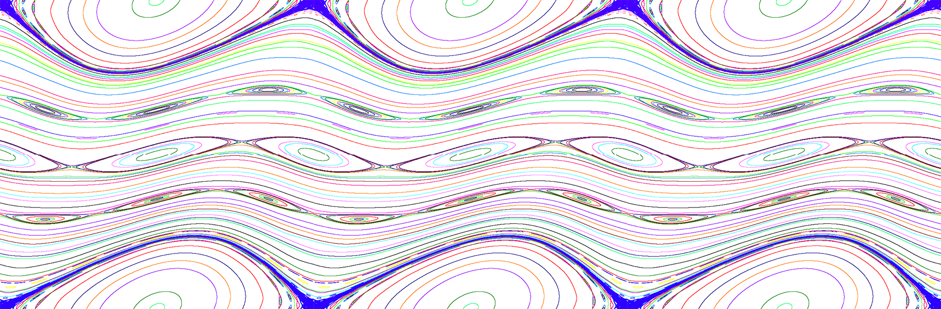
Figure 1. An example for $q=3$.

3. Preliminaries

In this section we review some basic terminology.

A Fréchet space $X$ is defined to be a complete metrizable locally convex topological vector space. Its topology may be induced by a family of seminorms $\{\|\cdot\|_{r}\}_{r}$. A Fréchet space $X$ is graded if the topology is defined by a family of semi-norms $\{\|\cdot\|_{r}\}_{r}$ satisfying $\|x\|_{s}\leqslant\|x\|_{t}$ for every $x\in X$ and $s\leqslant t$. For example, the space $C^{\infty}(\mathbb{T}^{d},\mathbb{R})$ with the topology given by the $C^{r}$ semi-norms $|g|_{r}=\max_{|j|=r}\sup_{z\in\mathbb{T}^{d}}|\partial^{j}g(z)|$, $r\in\mathbb{N}$ is a Fréchet space. By summing up the first $i$ semi-norms for every $i\in\mathbb{N}$, it turns $C^{\infty}(\mathbb{T}^{d},\mathbb{R})$ into a graded Fréchet space.

Our method of this paper shall use some approximation properties and quantitive estimates, e.g. the smoothing operators, the interpolation inequalities and the regularity of the composition operator. In particular, we need to control the norm of a function in the scale of Hölder spaces.

Now, let us turn to define Hölder regularities. For our purpose, it is sufficient to consider a convex set $U=\mathbb{T}\times E$ or $\mathbb{T}$ or $E$, with $E\subset\mathbb{R}$ an open interval, and then study the Hölder regularities of functions defined on $U$.

For $\lambda\in(0,1)$, we denote by $C^{\lambda}(U,\mathbb{R})$ the space of bounded $\lambda$-Hölder functions $g:U\to\mathbb{R}$ with the following norm

$$\|g\|_{\lambda}:=\max\left\{\|g(x)\|_{C^{0}},\quad\sup_{0<|z-z^{\prime}|\leqslant 1}\frac{|g(z)-g(z^{\prime})|}{|z-z^{\prime}|^{\lambda}}\right\}.$$

For integer $p\in\mathbb{N}$, $C^{p}(U,\mathbb{R})$ denotes the space of functions with continuous derivatives up to $p$ with the following norm

$$\|g\|_{p}:=\max_{0\leqslant t\leqslant p}\max_{|j|=t}\,\|\partial^{j}g\|_{C^{0}}.$$

For $\ell=p+\lambda$ with $p\in\mathbb{N}$ and $\lambda\in(0,1)$, we denote by $C^{\ell}(U,\mathbb{R})$ the space of functions $f:U\to\mathbb{R}$ with continuous derivatives up to $p$ and Hölder continuous partial derivatives $\partial^{j}f$ for all multi-indices $j$ satisfying $|j|=p$. We define its norm by

$$\|g\|_{\ell}:=\max\left\{\|g\|_{p},~{}\max_{|j|=p}\|\partial^{j}g\|_{\lambda}\right\}.$$

Here, following [SZ89], we have used the restriction $0<|z-z^{\prime}|\leqslant 1$ for the Hölder part of the norm. In this context, an immediate observation is that for any $f\in C^{r}(U,\mathbb{R})$, we have

$$\|f\|_{r}\geqslant\|f\|_{s},\qquad\text{ for all~{}}r\geqslant s\geqslant 0.$$

Indeed, this can be readily verified using the mean value theorem, since the domain $U$ is convex.

In consequence, we find that the space $C^{\infty}(U,\mathbb{R})$ of smooth functions with the family of Hölder norms $\{\|\cdot\|_{r}\}_{r\geqslant 0}$ is a graded Fréchet space.

Throughout this paper, the $C^{r}$ norm of a vector-valued function $G\in C^{\infty}(U,\mathbb{R}^{l})$ is defined by

$$\|G\|_{r}:=\max_{1\leqslant i\leqslant l}\|g_{i}\|_{r},$$

where $g_{i}\in C^{\infty}(U,\mathbb{R})$ is the $i$-th coordinate function of $G=(g_{1},\cdots,g_{l})$.

4. Initial reduction

In this section we will show that the proof of Theorem A can be reduced to that of Theorem 4.1. The basic idea is simple: since $\omega(y)$ is non-degenerate, the map $\mathcal{F}$ can be transformed into a simplified form which is just a perturbation of the standard integrable map $U_{0}(x,y)=(x+y,y)$.

Recall that the frequency map $\omega(y):\mathbb{R}\longrightarrow\mathbb{R}$ is a smooth diffeomorphism, with its inverse denoted by $\omega^{-1}(y)$. Define a smooth diffeomorphism $Q$ by

$$Q:~{}\mathbb{T}\times\mathbb{R}\longrightarrow\mathbb{T}\times\mathbb{R},\quad(x,y)\longmapsto(x,\omega^{-1}(y)),$$

and its inverse is

$$Q^{-1}:~{}\mathbb{T}\times\mathbb{R}\longrightarrow\mathbb{T}\times\mathbb{R},\quad(x,y)\longmapsto(x,\omega(y)).$$

Under the change of coordinates by $Q$, the unperturbed map $\mathcal{F}_{0}$ can be transformed into

$$U_{0}=Q^{-1}\circ\mathcal{F}_{0}\circ Q :~{}\mathbb{T}\times\mathbb{R}\longrightarrow\mathbb{T}\times\mathbb{R}$$

$$U_{0}(x,y) =(x+y,y).$$

Meanwhile, it is easily seen that $T_{\alpha}$ is invariant under the conjugacy $Q$, that is

$$Q^{-1}\circ T_{\alpha}\circ Q=T_{\alpha}.$$

For the maps $\mathcal{F}$ and $\mathcal{K}$ considered in Theorem A, under the coordinate transformation $Q$ we obtain the corresponding conjugated maps

$$\mathbf{F}=Q^{-1}\circ\mathcal{F}\circ Q:~{}\mathbb{T}\times\mathbb{R}\longrightarrow\mathbb{T}\times\mathbb{R}.$$

$$\mathbf{K}=Q^{-1}\circ\mathcal{K}\circ Q:~{}\mathbb{T}\times\mathbb{R}\longrightarrow\mathbb{T}\times\mathbb{R}.$$

More precisely, $\mathbf{F}=U_{0}+\mathbf{f}$ and $\mathbf{K}=T_{\alpha}+\mathbf{k}$ for some $\mathbf{f},\mathbf{k}\in C^{\infty}(\mathbb{T}\times\mathbb{R},\mathbb{R}^{2})$, and

$$\mathbf{F}(x,y)=(x+y+\mathbf{f}_{1}(x,y),~{}y+\mathbf{f}_{2}(x,y)),$$ (4.1)

where $\mathbf{f}_{1}=f_{1}\circ Q$ and $\mathbf{f}_{2}(x,y)=\omega(\omega^{-1}(y)+f_{2}\circ Q(x,y))-y$.

$$\mathbf{K}(x,y)=(x+\alpha+\mathbf{k}_{1}(x,y),~{}y+\mathbf{k}_{2}(x,y)),$$ (4.2)

where $\mathbf{k}_{1}=k_{1}\circ Q$ and $\mathbf{k}_{2}(x,y)=\omega(\omega^{-1}(y)+k_{2}\circ Q(x,y))-y$.

It is easy to verify the following facts.

Lemma 4.1.

The commutativity $\mathbf{F}\circ\mathbf{K}=\mathbf{K}\circ\mathbf{F}$ holds. $\mathbf{F}$ satisfies the intersection property. $\mathbf{K}$ is Lipschitz semi-conjugate to $R_{\alpha}$.

In fact, the commutativity of $\mathbf{F}$ and $\mathbf{K}$ follows directly from that of $\mathcal{F}$ and $\mathcal{K}$. The intersection property and the Lipschitz semi-conjugacy property are both preserved under coordinate transformations.

Therefore, by what we have shown above, Theorem A reduces to the following theorem.

Theorem 4.1.

Let $\mathbf{F},\mathbf{K}\in\textup{Diff}_{0}^{\infty}(\mathbb{T}\times\mathbb{R})$ be commuting diffeomorphisms which are induced by $\mathbf{F}=U_{0}+\mathbf{f}$ and $\mathbf{K}=T_{\alpha}+\mathbf{k}$, where $\mathbf{f},\mathbf{k}\in C^{\infty}(\mathbb{T}\times\mathbb{R},\mathbb{R}^{2})$ and $\alpha\in\mathrm{DC}(\sigma,\tau)$. Suppose that

• $\mathbf{F}$ satisfies the intersection property.

• $\mathbf{K}$ is Lipschitz semi-conjugate to the rigid circle rotation $R_{\alpha}$.

Then, there exists $\mu=\mu(\tau)>0$ such that: for any $\delta>0$ and any bounded open interval $\mathcal{I}\subset\mathbb{R}$, if the perturbations

$$\left\|\mathbf{f},~{}\mathbf{k}\right\|_{C^{\mu}(\mathbb{T}\times\mathcal{I}_{\delta})}<\varepsilon_{0}$$

for a sufficiently small $\varepsilon_{0}=\varepsilon_{0}(\tau,\mathcal{I},\delta)>0$, then $\mathbf{F}$ and $\mathbf{K}$ can be simultaneously $C^{\infty}$-conjugated to $U_{0}$ and $T_{\alpha}$ on $\mathbb{T}\times\mathcal{I}$, in the sense that there exists a $C^{\infty}$ diffeomorphism $H$ from $\mathbb{T}\times\mathcal{I}$ onto its image such that

$$H^{-1}\circ\mathbf{F}\circ H=U_{0},\qquad H^{-1}\circ\mathbf{K}\circ H=T_{\alpha}.$$

We remark that in the above theorem, $\mathcal{I}_{\delta}:=\{y\in\mathbb{R},~{}\textup{dist}(y,\mathcal{I})<\delta\}$. For simplicity we have used the notation

$$\|\mathbf{f},~{}\mathbf{k}\|_{C^{\mu}(\mathbb{T}\times\mathcal{I}_{\delta})}\overset{\textup{def}}{=}\max\{\|\mathbf{f}\|_{C^{\mu}(\mathbb{T}\times\mathcal{I}_{\delta})},~{}\|\mathbf{k}\|_{C^{\mu}(\mathbb{T}\times\mathcal{I}_{\delta})}\}.$$

$C^{\infty}(\mathbb{T}\times\mathbb{R},\mathbb{R}^{2})$ is the set of functions $\phi(x,y)\in C^{\infty}(\mathbb{R}\times\mathbb{R},\mathbb{R}^{2})$ that are $1$-periodic in $x$.

The following sections will be devoted to prove Theorem 4.1.

5. Linearized conjugacy equations and the commutativity

5.1. Linearized conjugacy equations

Let us focus on the commuting diffeomorphisms $\mathbf{F}=U_{0}+\mathbf{f}$ and $\mathbf{K}=T_{\alpha}+\mathbf{k}$ obtained in (4.1) and (4.2). In our setting, the simultaneous $C^{\infty}$-linearization problem amounts to find a smooth near-identity conjugacy $H=\textup{id}+\mathbf{h}$, with $\mathbf{h}(x,y)=(\mathbf{h}_{1}(x,y),\mathbf{h}_{2}(x,y))$ such that

$$\mathbf{K}\circ H=H\circ T_{\alpha},\qquad\mathbf{F}\circ H=H\circ U_{0}.$$

Since $\mathbf{K}=T_{\alpha}+\mathbf{k}$, the conjugacy equation $\mathbf{K}\circ H=H\circ T_{\alpha}$ is reduced to

$$\mathbf{h}\circ T_{\alpha}-\mathbf{h}=\mathbf{k}\circ H.$$ (5.1)

Simultaneously, as $\mathbf{F}=U_{0}+\mathbf{f}$, the conjugacy equation $\mathbf{F}\circ H=H\circ U_{0}$ is reduced to

$$\left\{\begin{array}[]{lll}\mathbf{h}_{1}\circ U_{0}-\mathbf{h}_{1}-\mathbf{h}_{2}&=\mathbf{f}_{1}\circ H\\ \mathbf{h}_{2}\circ U_{0}-\mathbf{h}_{2}&=\mathbf{f}_{2}\circ H.\end{array}\right.$$ (5.4)

There is no direct way to solve the nonlinear equations (5.1)-(5.4). Instead, we will use a KAM iterative scheme to solve this nonlinear problem. In other words, the solution is the limit of successive approximations obtained by approximating the nonlinear problem by its linear part, and solving approximately the corresponding linearized equation.

To simplify the notation, for any convex domain $E\subset\mathbb{R}$ we define two linear operators on $C^{\infty}(\mathbb{T}\times E,\mathbb{R}^{2})$ as follows: for $u(x,y)=(u_{1}(x,y),u_{2}(x,y))$,

$$\Delta_{\alpha}:~{}C^{\infty}(\mathbb{T}\times E,\mathbb{R}^{2}) \longrightarrow C^{\infty}(\mathbb{T}\times E,\mathbb{R}^{2})$$ (5.5)

$$u \longmapsto u\circ T_{\alpha}-u,$$

where $T_{\alpha}(x,y)=(x+\alpha,y)$, and

$$\Delta_{U_{0}}:~{}C^{\infty}(\mathbb{T}\times E,\mathbb{R}^{2}) \longrightarrow C^{\infty}(\mathbb{T}\times E,\mathbb{R}^{2})$$ (5.6)

$$u=\left(\begin{array}[]{ll}u_{1}\\ u_{2}\end{array}\right) \longmapsto\left(\begin{array}[]{ll}u_{1}\circ U_{0}-u_{1}-u_{2}\\ u_{2}\circ U_{0}-u_{2}\end{array}\right),$$

where $U_{0}(x,y)=(x+y,y)$. It is easily seen that the two linear operators commute, i.e.,

$$\Delta_{U_{0}}\Delta_{\alpha}=\Delta_{\alpha}\Delta_{U_{0}}.$$

Now, the corresponding linearized equations of (5.1)–(5.4) can be written as

$$\Delta_{\alpha}\mathbf{h} =\mathbf{k}$$ (5.7)

$$\Delta_{U_{0}}\mathbf{h} =\mathbf{f}$$ (5.8)

where $\mathbf{h}=(\mathbf{h}_{1},\mathbf{h}_{2})$, $\mathbf{k}=(\mathbf{k}_{1},\mathbf{k}_{2})$ and $\mathbf{f}=(\mathbf{f}_{1},\mathbf{f}_{2})$.

The basic idea of finding a common approximate solution is as follows. Thanks to the Diophantine property of $\alpha$, one can first obtain a solution $\mathbf{h}$ to equation (5.7). Then, by exploiting the commutativity relation we can show that $\mathbf{h}$ also solves equation (5.8) up to a higher order error. This idea is inspired by Moser’s commuting mechanism [Mos90].

For our purpose, we first give the following lemma for the linear operator $\Delta_{\alpha}$. It can be proved using Fourier analysis. We repeat the argument here for completeness. We also remark that the norm of the functions are in the scale of Hölder spaces.

Lemma 5.1.

Let $\alpha\in\mathrm{DC}(\sigma,\tau)$ and $E\subset\mathbb{R}$ be a convex open set. Given $\varphi(x,y)\in C^{\infty}(\mathbb{T}\times E,\mathbb{R})$, there is a unique solution $u\in C^{\infty}(\mathbb{T}\times E,\mathbb{R})$ satisfying $\int_{\mathbb{T}}u(x,y)\,dx=0$ such that

$$\Delta_{\alpha}u(x,y)=\varphi(x,y)-\int_{\mathbb{T}}\varphi(x,y)\,dx.$$ (5.9)

Moreover, for all real number $r\in[0,\infty)$ the solution $u$ satisfies

$$\left\|u\right\|_{r}\leqslant C\left\|\varphi\right\|_{r+\varrho},\qquad\varrho=[\tau]+2,$$ (5.10)

where the constant $C=C(\tau,\sigma)=\frac{1}{\sigma}\sum_{m\neq 0}\frac{1}{|m|^{2+[\tau]-\tau}}$, and $[\tau]$ is the integer part of $\tau>0$. For $r\notin\mathbb{N}$ we use the Hölder norm (see Section 3).

Remark 5.1.

The constant $C$ can be independent of $\tau$ if one choose $\varrho=\tau+2$ instead of $[\tau]+2$. Sometimes, the linear equation of the form (5.9) is also called a cohomological equation.

Proof.

Using Fourier series equation (5.9) becomes

$$\sum_{m\in\mathbb{Z}\setminus\{0\}}\left(e^{i2\pi m\alpha}-1\right)\widehat{u}_{m}(y)\,e^{i2\pi mx}=\sum_{m\in\mathbb{Z}\setminus\{0\}}\widehat{\varphi}_{m}(y)\,e^{i2\pi mx}$$

where the Fourier coefficients $\widehat{\varphi}_{m}(y)=\int_{\mathbb{T}}\varphi(\theta,y)e^{-i2\pi m\theta}\,d\theta$. Then we formally have a solution

$$u(x,y)=\sum_{m\in\mathbb{Z}\setminus\{0\}}\frac{\widehat{\varphi}_{m}(y)}{e^{i2\pi m\alpha}-1}e^{i2\pi mx}.$$

Observe that for each $m$,

$$\widehat{\varphi}_{m}(y)e^{i2\pi mx}=\int_{\mathbb{T}}\varphi(\theta,y)e^{-i2\pi m(\theta-x)}\,d\theta=\int_{\mathbb{T}}\varphi(\theta+x,y)e^{-i2\pi m\theta}\,d\theta.$$ (5.11)

Using integration by parts, we thus obtain

$$\left\|\widehat{\varphi}_{m}(y)e^{i2\pi mx}\right\|_{p}\leqslant\frac{1}{(2\pi)^{q}}\frac{\|\varphi\|_{p+q}}{|m|^{q}}\leqslant\frac{\|\varphi\|_{p+q}}{|m|^{q}},\qquad\text{for all ~{}}p,q\in\mathbb{N}.$$ (5.12)

Meanwhile, for each $m$ the following Hölder norm estimate holds

$$\left\|\widehat{\varphi}_{m}(y)e^{i2\pi mx}\right\|_{p+\lambda}\leqslant\frac{\|\varphi\|_{p+q+\lambda}}{|m|^{q}},\qquad\text{for all ~{}}p,q\in\mathbb{N},\quad\lambda\in(0,1).$$ (5.13)

To verify this estimate, we define $G(x,y)=\widehat{\varphi}_{m}(y)\,e^{i2\pi mx}$ for simplicity. Recall that

$$\left\|G\right\|_{p+\lambda}=\max\left\{\left\|G\right\|_{p},~{}\max_{|J|=p}\left\|\partial^{J}G\right\|_{\lambda}\right\}$$

where the multi-index $J=(J_{1},J_{2})\in\mathbb{N}^{2}$ and $\partial^{J}=\partial^{J_{1}}_{x}\partial^{J_{2}}_{y}$. Since by (5.12)

$$\|G\|_{p}\leqslant\frac{\|\varphi\|_{p+q}}{|m|^{q}}\leqslant\frac{\|\varphi\|_{p+q+\lambda}}{|m|^{q}},$$

it remains to check the Hölder norm $\left\|\partial^{J}G\right\|_{\lambda}$ for every multi-index $J$ satisfying $|J|=p$. In fact, by (5.11), for any two points $(x_{1},y_{1})$ and $(x_{2},y_{2})$,

$$\left|\partial^{J}G(x_{1},y_{1})-\partial^{J}G(x_{2},y_{2})\right|$$

$$= \left|\int_{\mathbb{T}}\left(\partial^{J}\varphi(\theta+x_{1},y_{1})-\partial^{J}\varphi(\theta+x_{2},y_{2})\right)e^{-i2\pi m\theta}\,d\theta\right|$$

$$\leqslant \frac{1}{|m|^{q}}\left|\int_{\mathbb{T}}\left(\partial^{J}\partial_{x}^{q}\varphi(\theta+x_{1},y_{1})-\partial^{J}\partial_{x}^{q}\varphi(\theta+x_{2},y_{2})\right)\,e^{-i2\pi m\theta}\,d\theta\right|$$

$$\leqslant \frac{1}{|m|^{q}}\,\sup_{\theta}\,\left|\partial^{J}\partial_{x}^{q}\varphi(\theta+x_{1},y_{1})-\partial^{J}\partial_{x}^{q}\varphi(\theta+x_{2},y_{2})\right|$$ (5.14)

Here, we have used integration by parts for the third line. As $|J|=p$, we infer from (5.14) that

$$\left\|\partial^{J}G\right\|_{\lambda}= \sup\limits_{0<\|(x_{1},y_{1})-(x_{2},y_{2})\|\leqslant 1}\frac{\left|\partial^{J}G(x_{1},y_{1})-\partial^{J}G(x_{2},y_{2})\right|}{\|(x_{1},y_{1})-(x_{2},y_{2})\|^{\lambda}}$$

$$\leqslant \frac{1}{|m|^{q}}\cdot\sup\limits_{0<\|(x_{1},y_{1})-(x_{2},y_{2})\|\leqslant 1}\frac{\|\varphi\|_{p+q+\lambda}\cdot\|(x_{1},y_{1})-(x_{2},y_{2})\|^{\lambda}}{\|(x_{1},y_{1})-(x_{2},y_{2})\|^{\lambda}}$$

$$\leqslant \frac{1}{|m|^{q}}\|\varphi\|_{p+q+\lambda}.$$

This thus verifies the desired result (5.13).

Next, we will estimate the $C^{r}$ norm of the solution $u$ for any $r\geqslant 0$. By (5.12)–(5.13), for any real $r\in\mathbb{R}^{+}$ and $q\in\mathbb{N}$,

$$\left\|u\right\|_{r}\leqslant\sum_{m\in\mathbb{Z}\setminus\{0\}}\frac{\left\|\widehat{\varphi}_{m}(y)e^{i2\pi mx}\right\|_{r}}{|e^{i2\pi m\alpha}-1|}\leqslant\sum_{m\in\mathbb{Z}\setminus\{0\}}\frac{\|\varphi\|_{r+q}}{|m|^{q}\,|e^{i2\pi m\alpha}-1|}\leqslant\frac{1}{\sigma}\sum_{m\in\mathbb{Z}\setminus\{0\}}\frac{\|\varphi\|_{r+q}}{|m|^{q-\tau}},$$

where for the last inequality we have used the Diophantine condition $\alpha\in\mathrm{DC}(\sigma,\tau)$. Note that the series on the right hand side is convergent if and only if the integer $q$ satisfies $q-\tau>1$. Hence, we can choose $q=[\tau]+2$, then

$$\left\|u\right\|_{r}\leqslant\frac{1}{\sigma}\sum_{m\in\mathbb{Z}\setminus\{0\}}\frac{\|\varphi\|_{r+[\tau]+2}}{|m|^{2+[\tau]-\tau}}\leqslant C(\tau,\sigma)\cdot\|\varphi\|_{r+[\tau]+2},$$

where the constant $C(\tau,\sigma)=\frac{1}{\sigma}\sum_{m\neq 0}\frac{1}{|m|^{2+[\tau]-\tau}}<\infty$ depends on $\tau$ and $\sigma$. This therefore proves estimate (5.10) for any real $r\geqslant 0$. This finishes the proof. ∎

This lemma tells us that given a differentiable function $\varphi$, the cohomological equation $\Delta_{\alpha}u=\varphi-[\varphi]$ has a solution, which in general is of lower regularity than $\varphi$. However, the loss of regularity can be controlled by the Diophantine exponent $\tau$. In particular, the solution $u\in C^{\infty}$ if $\varphi\in C^{\infty}$.

5.2. The commutativity property

Now we investigate the commutativity assumption.

Suppose that $\mathbf{F}=U_{0}+\mathbf{f}$ commutes with $\mathbf{K}=T_{\alpha}+\mathbf{k}$ on $\mathbb{T}\times E$ with $E\subset\mathbb{R}$ being convex and open. Then the commutation relation $\mathbf{F}\circ\mathbf{K}=\mathbf{K}\circ\mathbf{F}$ implies

$$\mathbf{f}_{1}\circ\mathbf{K}-\mathbf{f}_{1} =\mathbf{k}_{1}\circ\mathbf{F}-\mathbf{k}_{1}-\mathbf{k}_{2}$$ (5.15)

$$\mathbf{f}_{2}\circ\mathbf{K}-\mathbf{f}_{2} =\mathbf{k}_{2}\circ\mathbf{F}-\mathbf{k}_{2}$$

on $\mathbb{T}\times E$.

In view of the linear operators $\Delta_{\alpha}$ and $\Delta_{U_{0}}$ defined in (5.5)–(5.6), we also introduce a new linear operator

$$\mathcal{L}:C^{\infty}(\mathbb{T}\times E,\mathbb{R}^{2})\times C^{\infty}(\mathbb{T}\times E,\mathbb{R}^{2})\longrightarrow C^{\infty}(\mathbb{T}\times E,\mathbb{R}^{2})$$

given by

$$\mathcal{L}(f,g)\overset{\Delta}{=}\Delta_{U_{0}}\,g-\Delta_{\alpha}\,f.$$ (5.16)

In what follows, for a smooth function $\psi(x,y)$ we use $[\psi](y)$ to denote the average (or mean value) of $\psi$ over $\mathbb{T}$, that is

$$[\psi](y)=\int_{\mathbb{T}}\psi(x,y)\,dx.$$

In fact, this is exactly the $0$-th Fourier coefficient $\widehat{\psi}_{0}(y)$ of $\psi(x,y)=\sum\widehat{\psi}_{m}(y)e^{i2\pi mx}$.

For our maps $\mathbf{F}=U_{0}+\mathbf{f}$ and $\mathbf{K}=T_{\alpha}+\mathbf{k}$, the following result states that $\mathcal{L}(\mathbf{f},\mathbf{k})$ and the average $[\mathbf{k}_{2}]$ are both of higher order with respect to the size of the perturbations $\mathbf{f}$ and $\mathbf{k}$. This is essentially due to the commutativity property.

Lemma 5.2.

If $\mathbf{F}=U_{0}+\mathbf{f}$ commutes with $\mathbf{K}=T_{\alpha}+\mathbf{k}$, then the following estimates hold:

$$\|\mathcal{L}(\mathbf{f},\mathbf{k})\|_{r}\leqslant C_{r}\big{(}\|\mathbf{f}\|_{r+1}\,\|\mathbf{k}\|_{r}+\|\mathbf{k}\|_{r+1}\,\|\mathbf{f}\|_{r}\big{)},\qquad\textup{for any}~{}r\geqslant 0$$ (5.17)

$$\|~{}[\mathbf{k}_{2}]~{}\|_{0}\leqslant \|\mathbf{f}\|_{1}\,\|\mathbf{k}\|_{0}+\|\mathbf{k}\|_{1}\,\|\mathbf{f}\|_{0}\,,$$ (5.18)

where $[\mathbf{k}_{2}](y)$ is the average (over $\mathbb{T}$) of the second component of $\mathbf{k}=(\mathbf{k}_{1},\mathbf{k}_{2})$.

Proof.

The commutation relation gives (5.15), which can be rewritten as

$$\Delta_{U_{0}}\mathbf{k}-\Delta_{\alpha}\mathbf{f}=\mathbf{f}\circ\mathbf{K}-\mathbf{f}\circ T_{\alpha}-\mathbf{k}\circ\mathbf{F}+\mathbf{k}\circ U_{0}$$ (5.19)

which means that

$$\mathcal{L}(\mathbf{f},\mathbf{k})= \mathbf{f}\circ\mathbf{K}-\mathbf{f}\circ T_{\alpha}-\mathbf{k}\circ\mathbf{F}+\mathbf{k}\circ U_{0}=\int_{0}^{1}D\mathbf{f}(T_{\alpha}+t\mathbf{k})\,\mathbf{k}-D\mathbf{k}(U_{0}+t\mathbf{f})\,\mathbf{f}\,dt.$$ (5.20)

Then,

$$\|\mathcal{L}(\mathbf{f},\mathbf{k})\|_{0} \leqslant\|D\mathbf{f}\|_{0}\,\|\mathbf{k}\|_{0}+\|D\mathbf{k}\|_{0}\,\|\mathbf{f}\|_{0}\leqslant\|\mathbf{f}\|_{1}\,\|\mathbf{k}\|_{0}+\|\mathbf{k}\|_{1}\,\|\mathbf{f}\|_{0}.$$

This verifies (5.17) for $r=0$. Based on (5.20), the $C^{r}$, $r\geqslant 1$, norm estimates can be proved similarly, see for example [DF19, Proposition A.2] or [Laz93, Appendix II].

Now, it remains to prove inequality (5.18). Indeed, taking the average over $\mathbb{T}$ on both sides of (5.19) we get

$$[\Delta_{U_{0}}\mathbf{k}]-[\Delta_{\alpha}\mathbf{f}]=\int_{\mathbb{T}}\mathbf{f}_{1}\circ\mathbf{K}(x,y)-\mathbf{f}_{1}\circ T_{\alpha}(x,y)-\mathbf{k}_{1}\circ\mathbf{F}(x,y)+\mathbf{k}_{1}\circ U_{0}(x,y)\,dx.$$ (5.21)

Here, by (5.6) it follows that

$$[\Delta_{U_{0}}\mathbf{k}]=\left(\begin{array}[]{ll}\int_{\mathbb{T}}\mathbf{k}_{1}(x+y,y)\,dx-\int_{\mathbb{T}}\mathbf{k}_{1}(x,y)\,dx-\int_{\mathbb{T}}\mathbf{k}_{2}(x,y)\,dx\\ \int_{\mathbb{T}}\mathbf{k}_{2}(x+y,y)\,dx-\int_{\mathbb{T}}\mathbf{k}_{2}(x,y)\,dx\end{array}\right)=\left(\begin{array}[]{ll}-[\mathbf{k}_{2}]\\ 0\end{array}\right).$$

Similarly, we can show that $[\Delta_{\alpha}\mathbf{f}]=(0,0)$. Thus, (5.21) implies that

$$-[\mathbf{k}_{2}](y)=\int_{\mathbb{T}}\mathbf{f}_{1}\circ\mathbf{K}(x,y)-\mathbf{f}_{1}\circ T_{\alpha}(x,y)-\mathbf{k}_{1}\circ\mathbf{F}(x,y)+\mathbf{k}_{1}\circ U_{0}(x,y)\,dx,$$

which yields

$$\|[\mathbf{k}_{2}]\|_{0}\leqslant\|D\mathbf{f}_{1}\|_{0}\|\,\mathbf{k}\|_{0}+\|D\mathbf{k}_{1}\|_{0}\,\|\mathbf{f}\|_{0}\leqslant\|\mathbf{f}\|_{1}\,\|\mathbf{k}\|_{0}+\|\mathbf{k}\|_{1}\,\|\mathbf{f}\|_{0}.$$

This finishes the proof. ∎

We end this section by mentioning an interesting result [Tru21] which reveals some connection between the commutativity and the KAM set for the analytic systems. It shows that for two nearly integrable and exact symplectic $C^{\omega}$ maps, if the image of the KAM curves of the two maps intersect on a $C^{\infty}$-uniqueness set, then the two maps commute.

5.3. Smoothing operators

As we can see from estimate (5.10) in Lemma 5.1, the $C^{r}$ norm of the solution $u$ can be estimated by the $C^{r+\varrho}$ norm of $\varphi$, with a fixed loss of regularity $\varrho=[\tau]+2$. For our KAM iterative scheme in the following sections, we shall choose an appropriate smoothing operator to compensate for this fixed loss of regularity at each iterative step. By using interpolation inequalities, one can recover good behavior of some intermediate norms. Then the error introduced by this smoothing operator would not destroy the rapid convergence of the iteration (The convergence is not quadratic, but it is still faster than exponential). This idea comes from the Nash-Moser technique.

The following approximation result is well known. We refer to [Mos66, Zeh75, SZ89] for the proof and more details.

Lemma 5.3.

Let $E\subset\mathbb{R}$ be open and convex. There exists a family of linear smoothing operators $\{\mathrm{S}_{N}\}_{N\in\mathbb{R}^{+}}$ from $C^{\infty}(\mathbb{T}\times E,\mathbb{R})$ into itself, such that for every $\psi\in C^{\infty}(\mathbb{T}\times E,\mathbb{R})$, one has $\lim_{N\to\infty}\left\|\psi-\mathrm{S}_{N}\psi\right\|_{0}=0$, and

$$\left\|\mathrm{S}_{N}\psi\right\|_{l} \leqslant C_{s,l}N^{l-s}\left\|\psi\right\|_{s}\qquad\text{for~{}}l\geqslant s,$$ (5.22)

and for the linear operator $\mathrm{R}_{N}\overset{\textup{def}}{=}\textup{id}-\mathrm{S}_{N}$, it satisfies

$$\left\|\mathrm{R}_{N}\psi\right\|_{s} \leqslant C_{s,l}\frac{\left\|\psi\right\|_{l}}{N^{l-s}}\qquad\text{for~{}}l\geqslant s.$$ (5.23)

Here, $C_{s,l}>0$ are constants depending on $s$ and $l$.

Remark 5.2.

In fact, the smoothing operators $\mathrm{S}_{N}$ are constructed by convoluting with appropriate kernels decaying rather fast at infinity. So, if $\psi$ is periodic in some variables then so are the approximating functions $\mathrm{S}_{N}\psi$ in the same variables. Moreover, by the definition of convolution, it is not difficult to check that $[\mathrm{S}_{N}\psi](y)=\mathrm{S}_{N}[\psi](y)$.

However, the operators $\mathrm{S}_{N}$ given in Lemma 5.3 may not preserve the averages, i.e., $[\mathrm{S}_{N}\psi](y)\neq[\psi](y)$ and $\mathrm{S}_{N}[\psi](y)\neq[\psi](y)$ in general.

We also note that for the functions defined on $\mathbb{T}\times E$, the Fourier truncation operators $S_{N}\psi(x,y)$ $=$ $\sum_{|m|\leqslant N}\widehat{\psi}_{m}(y)e^{i2\pi mx}$ are not smoothing operators. In fact, for Fourier truncation operators, although inequality (5.23) is still true, inequality (5.22) does not hold for the partial derivatives of $\psi$ with respect to $y$ (it holds only for the partial derivatives of $\psi$ with respect to $x$).

As pointed out in [Zeh75], one important consequence of the existence of smoothing operators is the interpolation inequalities (Hadamard convexity inequalities), which will be very useful to us later on.

Lemma 5.4.

[Zeh75] Let $g\in C^{\infty}(\mathbb{T}\times E,\mathbb{R})$ with $E\subset\mathbb{R}$ convex and open. Then, for all $s\leqslant m\leqslant l$, $m=(1-\lambda)s+\lambda l$ with $\lambda\in[0,1]$,

$$\left\|g\right\|_{m}\leqslant C_{\lambda,s,l}\left\|g\right\|_{s}^{1-\lambda}\left\|g\right\|_{l}^{\lambda},$$

where the constants $C_{\lambda,l,s}>0$ depend only on $l,s$ and $\lambda$.

In fact, as $s\leqslant m\leqslant l$, we choose $N\in\mathbb{R}^{+}$ satisfying $N^{l-s}=\frac{\|g\|_{l}}{\|g\|_{s}}$, and then invoke Lemma 5.3 to obtain that

$$\left\|g\right\|_{m}\leqslant\|\mathrm{S}_{N}g\|_{m}+\|\mathrm{R}_{N}g\|_{m}\leqslant C_{s,m}N^{m-s}\|g\|_{s}+C_{m,l}N^{m-l}\|g\|_{l}$$

$$= (C_{s,m}+C_{m,l})\|g\|^{\frac{l-m}{l-s}}_{s}\|g\|_{l}^{\frac{m-s}{l-s}}.$$

We also refer to [dlLO99] for a proof done by an elementary method, and extend even to Hölder spaces of functions defined in a Banach space [dlL01].

6. Inductive lemma and the error estimates

The goal of this section is to prove Proposition 6.1, which will be the main ingredient in the proof of Theorem 4.1. It allows us to obtain smaller errors after each iteration, which thus ensures the convergence of our KAM iteration scheme, see Section 7.

Let $\alpha\in\mathrm{DC}(\sigma,\tau)$, we recall the constant

$$\varrho=[\tau]+2$$

obtained in Lemma 5.1. Then the following result holds.

Proposition 6.1.

Let $\mathbf{F}=U_{0}+\mathbf{f}$ and $\mathbf{K}=T_{\alpha}+\mathbf{k}$ be commuting $C^{\infty}$ diffeomorphisms, where $\mathbf{F}$ has the intersection property. Let $\delta\in(0,\frac{1}{2}]$ and $\mathcal{I}\subset\mathbb{R}$ be a bounded open interval, we write $\|\mathbf{f},~{}\mathbf{k}\|_{r}=\|\mathbf{f},~{}\mathbf{k}\|_{C^{r}(\mathbb{T}\times\mathcal{I}_{\delta})}$. Suppose that $\mathbf{K}$ is semi-conjugate to $R_{\alpha}$ via a Lipschitz semi-conjugacy of the form $W(x,y)=x+v(x,y)$, where $v\in\textup{Lip}(\mathbb{T}\times\mathcal{I}_{\delta},\mathbb{R})$ satisfies $|v(z)-v(z^{\prime})|\leqslant\mathfrak{L}\cdot\textup{dist}(z,z^{\prime})$ for some $\mathfrak{L}>1$.

Then, for $N>1$, there exists $\mathbf{h}\in C^{\infty}(\mathbb{T}\times\mathcal{I}_{\delta},\mathbb{R}^{2})$, see formula (6.13), satisfying

$$\|\mathbf{h}\|_{r}\leqslant C_{r^{\prime},r,\varrho}\,N^{r-r^{\prime}+\varrho}\|\mathbf{f},~{}\mathbf{k}\|_{r^{\prime}},\qquad\text{for~{}}r\geqslant r^{\prime}\geqslant 0.$$ (6.1)

Denote $\theta=\|\mathbf{h}\|_{1}$, $\theta^{\prime}=\|\mathbf{f},~{}\mathbf{k}\|_{0}$ and assume that

$$\widetilde{\delta}:=\delta-2\theta-\theta^{\prime}>0,$$ (6.2)

then the map $H=\textup{id}+\mathbf{h}$ has a smooth inverse $H^{-1}$ defined on $\mathbb{T}\times\mathcal{I}_{\delta-\theta}$, and the conjugated maps

$$\widetilde{\mathbf{F}}=H^{-1}\circ\mathbf{F}\circ H,\qquad\widetilde{\mathbf{K}}=H^{-1}\circ\mathbf{K}\circ H,$$

are smooth diffeomorphisms from $\mathbb{T}\times\mathcal{I}_{\widetilde{\delta}}$ onto their images.

Writing $\widetilde{\mathbf{F}}=U_{0}+\widetilde{\mathbf{f}}$ and $\widetilde{\mathbf{K}}=T_{\alpha}+\widetilde{\mathbf{k}}$, where $\widetilde{\mathbf{f}},\widetilde{\mathbf{k}}\in C^{\infty}(\mathbb{T}\times\mathcal{I}_{\widetilde{\delta}},\mathbb{R}^{2})$, we have:

$$\left\|\widetilde{\mathbf{f}},~{}\widetilde{\mathbf{k}}\right\|_{0}\leqslant C_{r,\varrho}\cdot\mathfrak{L}\cdot\left(N^{2\varrho}\|\mathbf{f},~{}\mathbf{k}\|_{1}\,\|\mathbf{f},~{}\mathbf{k}\|_{0}+\frac{\|\mathbf{f},\mathbf{k}\|^{2}_{\varrho+r+1}}{N^{r}}+\frac{\|\mathbf{f},\mathbf{k}\|_{\varrho+r}}{N^{r}}\right),\quad\text{for~{}}r\geqslant 0,$$ (6.3)

$$\left\|\widetilde{\mathbf{f}},~{}\widetilde{\mathbf{k}}\right\|_{r}\leqslant C_{r,\varrho}\,\Big{(}1+N^{\varrho}\|\mathbf{f},~{}\mathbf{k}\|_{r}\Big{)},\qquad\text{for~{}}r>0.$$ (6.4)

Moreover, $\widetilde{\mathbf{K}}$ is semi-conjugate to $R_{\alpha}$ via a Lipschitz semi-conjugacy $\widetilde{W}(x,y)=x+\widetilde{v}(x,y)$, where $\widetilde{v}\in\textup{Lip}(\mathbb{T}\times\mathcal{I}_{\widetilde{\delta}},\mathbb{R})$ has a Lipschitz bound $\mathfrak{\widetilde{L}}>1$ satisfying

$$\mathfrak{\widetilde{L}}\leqslant\mathfrak{L}\,(1+2\|\mathbf{h}\|_{1}).$$ (6.5)

Remark 6.1.

In fact, to simplify the notation we have used

$$\|\mathbf{h}\|_{r}=\|\mathbf{h}\|_{C^{r}(\mathbb{T}\times\mathcal{I}_{\delta})},\qquad\left\|\widetilde{\mathbf{f}},~{}\widetilde{\mathbf{k}}\right\|_{r}=\left\|\widetilde{\mathbf{f}},~{}\widetilde{\mathbf{k}}\right\|_{C^{r}(\mathbb{T}\times\mathcal{I}_{\widetilde{\delta}})}.$$

Condition (6.2) implies that $\|\mathbf{f},~{}\mathbf{k}\|_{1}$ shall be suitably small.

The proof of Proposition 6.1 will be divided into several lemmas.

6.1. Construction of $\mathbf{h}$

The following lemma shows that the solution of the linearized equation $\Delta_{\alpha}u=\mathrm{S}_{N}\mathbf{k}-[\mathrm{S}_{N}\mathbf{k}]$ is, to some extent, an approximate solution of the linearized equation $\Delta_{U_{0}}u=\mathrm{S}_{N}\mathbf{f}-[\mathrm{S}_{N}\mathbf{f}]$. It is essentially due to the commutativity condition (see Lemma 5.2).

For simplicity we introduce the set

$$C_{0}^{\infty}(\mathbb{T}\times\mathcal{I}_{\delta},\mathbb{R}^{2})=\left\{\phi(x,y)\in C^{\infty}(\mathbb{T}\times\mathcal{I}_{\delta},\mathbb{R}^{2})~{}:~{}[\phi](y)=\int_{\mathbb{T}}\phi(x,y)\,dx=0\right\}.$$

Lemma 6.1.

Given $N>1$, there is a unique solution $\xi_{N}(x,y)\in C_{0}^{\infty}(\mathbb{T}\times\mathcal{I}_{\delta},\mathbb{R}^{2})$ to the following equation of $u$

$$\Delta_{\alpha}u=\mathrm{S}_{N}\mathbf{k}-[\mathrm{S}_{N}\mathbf{k}].$$ (6.6)

It satisfies

$$\|\xi_{N}\|_{r}\leqslant C_{r^{\prime},r+\varrho}N^{r-r^{\prime}+\varrho}\|\mathbf{k}\|_{r^{\prime}}\,,$$ (6.7)

for any $r\geqslant r^{\prime}\geqslant 0$. Moreover, if we define $\mathcal{N}$ by

$$\mathcal{N}(x,y)\overset{\textup{def}}{=}\Delta_{U_{0}}\xi_{N}(x,y)-\big{(}\mathrm{S}_{N}\mathbf{f}(x,y)-[\mathrm{S}_{N}\mathbf{f}](y)\big{)}.$$ (6.8)

Then,

$$\|\mathcal{N}\|_{0}\leqslant C_{\varrho,r}\left(N^{\varrho}\|\mathbf{f},~{}\mathbf{k}\|_{1}\|\mathbf{f},~{}\mathbf{k}\|_{0}+\frac{\|\mathbf{f},\mathbf{k}\|^{2}_{\varrho+r+1}}{N^{r}}+\frac{\|\mathbf{f},\mathbf{k}\|_{\varrho+r}}{N^{r}}\right),\quad\textup{for}~{}r\geqslant 0.$$ (6.9)

Proof.

By Lemma 5.1, there is a unique solution denoted by $\xi_{N}(x,y)\in C_{0}^{\infty}(\mathbb{T}\times\mathcal{I}_{\delta},\mathbb{R}^{2})$ to the linear equation (6.6), and by estimate (5.10), it follows that $\|\xi_{N}\|_{r}\leqslant C\|\mathrm{S}_{N}\mathbf{k}\|_{r+\varrho}$. Then, due to Lemma 5.3 we have

$$\|\xi_{N}\|_{r}\leqslant C_{r^{\prime},r+\varrho}N^{r-r^{\prime}+\varrho}\|\mathbf{k}\|_{r^{\prime}}\,,$$

for any $r\geqslant r^{\prime}\geqslant 0$. Next, we consider the function $\mathcal{N}$. Recall that the smoothing operators $\mathrm{S}_{N}$ are constructed by the convolution, it is easy to find that every $\mathrm{S}_{N}$ commutes with the operator $\Delta_{\alpha}$, and $\Delta_{\alpha}$ also commutes with $\Delta_{U_{0}}$, namely

$$\Delta_{\alpha}\Delta_{U_{0}}=\Delta_{U_{0}}\Delta_{\alpha},\quad\Delta_{\alpha}\,\mathrm{S}_{N}=\mathrm{S}_{N}\,\Delta_{\alpha}.$$

Then $\mathcal{N}$ satisfies the following equation

$$\Delta_{\alpha}\mathcal{N}=\Delta_{\alpha}\Delta_{U_{0}}\xi_{N}-\Delta_{\alpha}\mathrm{S}_{N}\mathbf{f}+\Delta_{\alpha}[\mathrm{S}_{N}\mathbf{f}]= \Delta_{U_{0}}\Delta_{\alpha}\xi_{N}-\Delta_{\alpha}\mathrm{S}_{N}\mathbf{f}$$ (6.10)

$$= \Delta_{U_{0}}(\mathrm{S}_{N}\mathbf{k}-[\mathrm{S}_{N}\mathbf{k}])-\Delta_{\alpha}\mathrm{S}_{N}\mathbf{f}$$

$$= \Delta_{U_{0}}\mathrm{S}_{N}\mathbf{k}-\Delta_{U_{0}}[\mathrm{S}_{N}\mathbf{k}]-\Delta_{\alpha}\mathrm{S}_{N}\mathbf{f}$$

$$= \mathcal{L}(\mathrm{S}_{N}\mathbf{f},\mathrm{S}_{N}\mathbf{k})-\Delta_{U_{0}}[\mathrm{S}_{N}\mathbf{k}].$$

See also (5.16) for the definition of $\mathcal{L}$. Note that the average

$$[\mathcal{N}]=[\Delta_{U_{0}}\xi_{N}]= \left(\begin{array}[]{ll}\int_{\mathbb{T}}\xi_{N,1}(x+y,y)\,dx-\int_{\mathbb{T}}\xi_{N,1}(x,y)\,dx-\int_{\mathbb{T}}\xi_{N,2}(x,y)\,dx\\ \int_{\mathbb{T}}\xi_{N,2}(x+y,y)\,dx-\int_{\mathbb{T}}\xi_{N,2}(x,y)\,dx\end{array}\right)$$

$$= \left(\begin{array}[]{ll}-[\xi_{N,2}]\\ 0\end{array}\right)=\mathbf{0}$$

as a result of $\xi_{N}\in C_{0}^{\infty}(\mathbb{T}\times\mathcal{I}_{\delta},\mathbb{R}^{2})$. Thus, applying Lemma 5.1 to (6.10) we deduce that

$$\left\|\mathcal{N}\right\|_{0}\leqslant C\left\|~{}\mathcal{L}(\mathrm{S}_{N}\mathbf{f},\mathrm{S}_{N}\mathbf{k})-\Delta_{U_{0}}[\mathrm{S}_{N}\mathbf{k}]~{}\right\|_{\varrho}\,.$$

Since $\mathrm{S}_{N}=id-\mathrm{R}_{N}$, we have

$$\mathcal{L}(\mathrm{S}_{N}\mathbf{f},\mathrm{S}_{N}\mathbf{k})= \mathcal{L}(\mathbf{f},\mathbf{k})-\Delta_{U_{0}}\mathrm{R}_{N}\mathbf{k}+\Delta_{\alpha}\mathrm{R}_{N}\mathbf{f}$$

$$= \mathrm{S}_{N}\mathcal{L}(\mathbf{f},\mathbf{k})+\mathrm{R}_{N}\mathcal{L}(\mathbf{f},\mathbf{k})-\Delta_{U_{0}}\mathrm{R}_{N}\mathbf{k}+\Delta_{\alpha}\mathrm{R}_{N}\mathbf{f}.$$

Thus, by Lemma 5.3 and inequality (5.17) of Lemma 5.2 we deduce that: for any $r\geqslant 0$,

$$\|\mathcal{L}(\mathrm{S}_{N}\mathbf{f},\mathrm{S}_{N}\mathbf{k})\|_{\varrho} \leqslant C_{\varrho,r}\left(N^{\varrho}\|\mathcal{L}(\mathbf{f},\mathbf{k})\|_{0}+\frac{\|\mathcal{L}(\mathbf{f},\mathbf{k})\|_{\varrho+r}}{N^{r}}+\|\mathrm{R}_{N}\mathbf{k}\|_{\varrho}+\|\mathrm{R}_{N}\mathbf{f}\|_{\varrho}\right)$$

$$\leqslant C^{\prime}_{\varrho,r}\left(N^{\varrho}\|\mathbf{f},\mathbf{k}\|_{1}\|\mathbf{f},\mathbf{k}\|_{0}+\frac{\|\mathbf{f},\mathbf{k}\|_{\varrho+r+1}\|\mathbf{f},\mathbf{k}\|_{\varrho+r}}{N^{r}}+\frac{\|\mathbf{f},\mathbf{k}\|_{\varrho+r}}{N^{r}}\right)$$

$$\leqslant C^{\prime}_{\varrho,r}\left(N^{\varrho}\|\mathbf{f},\mathbf{k}\|_{1}\|\mathbf{f},\mathbf{k}\|_{0}+\frac{\|\mathbf{f},\mathbf{k}\|^{2}_{\varrho+r+1}}{N^{r}}+\frac{\|\mathbf{f},\mathbf{k}\|_{\varrho+r}}{N^{r}}\right).$$ (6.11)

Meanwhile, it is easy to check that $\Delta_{U_{0}}[\mathrm{S}_{N}\mathbf{k}]=(-[\mathrm{S}_{N}\mathbf{k}_{2}],0)$, then using Lemma 5.3 and the inequality (5.18) of Lemma 5.2,

$$\|\Delta_{U_{0}}[\mathrm{S}_{N}\mathbf{k}]\|_{\varrho}=\|~{}[\mathrm{S}_{N}\mathbf{k}_{2}]~{}\|_{\varrho}=\|~{}\mathrm{S}_{N}[\mathbf{k}_{2}]~{}\|_{\varrho}\leqslant C_{\varrho}\,N^{\varrho}\|~{}[\mathbf{k}_{2}]~{}\|_{0}$$

$$\leqslant C_{\varrho}N^{\varrho}\left(\|\mathbf{f}\|_{1}\|\mathbf{k}\|_{0}+\|\mathbf{k}\|_{1}\|\mathbf{f}\|_{0}\right).$$ (6.12)

Therefore, (6.11) together with (6.12) implies that

$$\left\|\mathcal{N}\right\|_{0}\leqslant C_{\varrho,r}\left(N^{\varrho}\|\mathbf{f},~{}\mathbf{k}\|_{1}\|\mathbf{f},~{}\mathbf{k}\|_{0}+\frac{\|\mathbf{f},\mathbf{k}\|^{2}_{\varrho+r+1}}{N^{r}}+\frac{\|\mathbf{f},\mathbf{k}\|_{\varrho+r}}{N^{r}}\right),\qquad\textup{for any}~{}r\geqslant 0.$$

∎

Based on the solution $\xi_{N}$ obtained in Lemma 6.1, we construct the near-identity conjugacy $H=\textup{id}+\mathbf{h}$ as follows:

$$\mathbf{h}\overset{\textup{def}}{=}\left(\begin{array}[]{r}0\\ -{[}\mathrm{S}_{N}\mathbf{f}_{1}{]}\end{array}\right)+\xi_{N}=\left(\begin{array}[]{r}\xi_{N,1}\\ -{[}\mathrm{S}_{N}\mathbf{f}_{1}{]}+\xi_{N,2}\end{array}\right),$$ (6.13)

where we write $\xi_{N}=(\xi_{N,1},\xi_{N,2})$. Note that $\Delta_{\alpha}[\mathrm{S}_{N}\mathbf{f}_{1}]=0$, so $\mathbf{h}\in C^{\infty}(\mathbb{T}\times\mathcal{I}_{\delta},\mathbb{R}^{2})$ is still a solution of (6.6), that is

$$\Delta_{\alpha}\mathbf{h}=\mathrm{S}_{N}\mathbf{k}-[\mathrm{S}_{N}\mathbf{k}].$$

However, the average $[\mathbf{h}]\neq 0$ in general.

Lemma 6.2.

$\mathbf{h}$ satisfies the following estimates.

$$\|\mathbf{h}\|_{r}\leqslant C_{r,\varrho}N^{\varrho}\|\mathbf{f},~{}\mathbf{k}\|_{r}\,,\qquad\text{for every~{} }r\geqslant 0.$$ (6.14)

$$\|\mathbf{h}\|_{r}\leqslant C_{r^{\prime},r,\varrho}N^{r-r^{\prime}+\varrho}\|\mathbf{f},~{}\mathbf{k}\|_{r^{\prime}}\,.\qquad\text{for every~{} }r\geqslant r^{\prime}\geqslant 0.$$ (6.15)

Moreover, under assumption (6.2), the map $H=\textup{id}+\mathbf{h}$ has a smooth inverse

$$H^{-1}:\mathbb{T}\times\mathcal{I}_{\delta-\theta}\longrightarrow\mathbb{T}\times\mathbb{R}$$

which is a smooth diffeomorphism from $\mathbb{T}\times\mathcal{I}_{\delta-\theta}$ onto its image, and $H^{-1}(\mathbb{T}\times\mathcal{I}_{\delta-\theta})$ $\subset$ $\mathbb{T}\times\mathcal{I}_{\delta}$.

Proof.

Applying Lemma 5.3 and inequality (6.7) to the formula (6.13),

$$\|\mathbf{h}\|_{r}\leqslant\|\mathrm{S}_{N}\mathbf{f}\|_{r}+\|\xi_{N}\|_{r}\leqslant C_{r^{\prime},r}N^{r-r^{\prime}}\|\mathbf{f}\|_{r^{\prime}}+C_{r^{\prime},r+\varrho}N^{r-r^{\prime}+\varrho}\|\mathbf{k}\|_{r^{\prime}}$$

$$\leqslant C_{r^{\prime},r,\varrho}N^{r-r^{\prime}+\varrho}\|\mathbf{f},~{}\mathbf{k}\|_{r^{\prime}}$$

for any $r\geqslant r^{\prime}\geqslant 0$, where the constant $C_{r^{\prime},r,\varrho}>0$ depends on $r^{\prime},r$ and $\varrho$. This proves the desired estimate (6.15). In particular, (6.14) follows immediately by taking $r=r^{\prime}$.

By assumption (6.2), we infer that $\theta=\|\mathbf{h}\|_{1}$ satisfies

$$\theta<\delta/2\leqslant\frac{1}{4}.$$

Then, Proposition A.1 implies that the map $H=\textup{id}+\mathbf{h}$ has a smooth inverse $H^{-1}$, which is a smooth diffeomorphism from $\mathbb{T}\times\mathcal{I}_{\delta-\theta}$ onto its image, and $H^{-1}(\mathbb{T}\times\mathcal{I}_{\delta-\theta})$ $\subset$ $\mathbb{T}\times\mathcal{I}_{\delta}$. ∎

6.2. $C^{0}$-norm estimates of the new errors

By assumption (6.2), $\theta=\|\mathbf{h}\|_{1}$ and $\theta^{\prime}=\|\mathbf{f},\mathbf{k}\|_{0}$ satisfies

$$\widetilde{\delta}:=\delta-2\theta-\theta^{\prime}>0.$$ (6.16)

Then, it is easy to find that $\mathbf{F}\circ H(\mathbb{T}\times\mathcal{I}_{\widetilde{\delta}})\subset\mathbb{T}\times\mathcal{I}_{\delta-\theta}$. According to Lemma 6.2, $H^{-1}$ is well defined on $\mathbb{T}\times\mathcal{I}_{\delta-\theta}$, we thus have the following conjugated map

$$\widetilde{\mathbf{F}}=H^{-1}\circ\mathbf{F}\circ H:~{}\mathbb{T}\times\mathcal{I}_{\widetilde{\delta}}\longrightarrow\mathbb{T}\times\mathbb{R}$$

which is a smooth diffeomorphism from $\mathbb{T}\times\mathcal{I}_{\widetilde{\delta}}$ onto its image. Similarly,

$$\widetilde{\mathbf{K}}=H^{-1}\circ\mathbf{K}\circ H:~{}\mathbb{T}\times\mathcal{I}_{\widetilde{\delta}}\longrightarrow\mathbb{T}\times\mathbb{R}$$

is also a smooth diffeomorphism from $\mathbb{T}\times\mathcal{I}_{\widetilde{\delta}}$ onto its image.

We write $\widetilde{\mathbf{F}}=U_{0}+\widetilde{\mathbf{f}}$ and $\widetilde{\mathbf{K}}=T_{\alpha}+\widetilde{\mathbf{k}}$, where $\widetilde{\mathbf{f}},\widetilde{\mathbf{k}}\in C^{\infty}(\mathbb{T}\times\mathcal{I}_{\widetilde{\delta}},\mathbb{R}^{2})$. We will show that the new errors $\|\widetilde{\mathbf{f}}\|_{0}$ and $\|\widetilde{\mathbf{k}}\|_{0}$ are of higher order. As we will see below, the hard part is the average terms. This is the only place where we need the intersection property and the Lipschitz semi-conjugacy condition.

Lemma 6.3.

For every $r\geqslant 0$,

$$\left\|\widetilde{\mathbf{f}}\right\|_{0}\leqslant C_{r,\varrho}\left(N^{\varrho}\|\mathbf{f},~{}\mathbf{k}\|_{1}\|\mathbf{f},~{}\mathbf{k}\|_{0}+\frac{\|\mathbf{f},\mathbf{k}\|^{2}_{\varrho+r+1}}{N^{r}}+\frac{\|\mathbf{f},\mathbf{k}\|_{\varrho+r}}{N^{r}}\right).$$ (6.17)

For $\widetilde{\mathbf{k}}=(\widetilde{\mathbf{k}}_{1},\widetilde{\mathbf{k}}_{2})$, it satisfies

$$\left\|\widetilde{\mathbf{k}}_{1}\right\|_{0}\leqslant C_{r,\varrho}\cdot\mathfrak{L}\cdot\left(N^{2\varrho}\|\mathbf{f},~{}\mathbf{k}\|_{1}\|\mathbf{f},~{}\mathbf{k}\|_{0}+\frac{\|\mathbf{k}\|_{r}}{N^{r}}\right),$$ (6.18)

$$\left\|\widetilde{\mathbf{k}}_{2}\right\|_{0}\leqslant C_{r,\varrho}\left(N^{2\varrho}\|\mathbf{f},~{}\mathbf{k}\|_{1}\|\mathbf{f},~{}\mathbf{k}\|_{0}+\frac{\|\mathbf{k}\|_{r}}{N^{r}}\right).$$ (6.19)

Here, $\mathfrak{L}>1$ is a Lipschitz bound of $v(x,y)$ for the semi-conjugacy $W(x,y)=x+v(x,y)$.

Proof.

We first consider $\widetilde{\mathbf{f}}$. Note that the identity $H\circ\widetilde{\mathbf{F}}=\mathbf{F}\circ H$ implies

$$\widetilde{\mathbf{f}}=U_{0}\circ H-U_{0}+\mathbf{f}\circ H-\mathbf{h}\circ\widetilde{\mathbf{F}}.$$

In light of $U_{0}(x,y)=(x+y,y)$ and $\mathbf{h}$ given in (6.13), we deduce that

$$\widetilde{\mathbf{f}}= \left(\begin{array}[]{l}\mathbf{h}_{1}+\mathbf{h}_{2}\\ \mathbf{h}_{2}\end{array}\right)+\mathbf{f}\circ H-\mathbf{h}\circ\widetilde{\mathbf{F}}$$

$$= -\Delta_{U_{0}}\mathbf{h}+\mathbf{h}\circ U_{0}+\mathbf{f}\circ H-\mathbf{h}\circ\widetilde{\mathbf{F}}$$

$$= -\Delta_{U_{0}}\mathbf{h}+\mathbf{f}+(\mathbf{f}\circ H-\mathbf{f}+\mathbf{h}\circ U_{0}-\mathbf{h}\circ\widetilde{\mathbf{F}})$$

$$= \left(\begin{array}[]{l}-[\mathrm{S}_{N}\mathbf{f}_{1}]\\ 0\end{array}\right)-\Delta_{U_{0}}\xi_{N}+\mathbf{f}+(\mathbf{f}\circ H-\mathbf{f}+\mathbf{h}\circ U_{0}-\mathbf{h}\circ\widetilde{\mathbf{F}})$$

$$= \left(\begin{array}[]{l}0\\ {[}\mathrm{S}_{N}\mathbf{f}_{2}{]}\end{array}\right)-\left([\mathrm{S}_{N}\mathbf{f}]+\Delta_{U_{0}}\xi_{N}-\mathrm{S}_{N}\mathbf{f}\right)+\mathrm{R}_{N}\mathbf{f}+(\mathbf{f}\circ H-\mathbf{f}+\mathbf{h}\circ U_{0}-\mathbf{h}\circ\widetilde{\mathbf{F}})$$

$$= \left(\begin{array}[]{l}0\\ {[}\mathrm{S}_{N}\mathbf{f}_{2}{]}\end{array}\right)-\mathcal{N}+(\mathrm{R}_{N}\mathbf{f}+\mathbf{f}\circ H-\mathbf{f}+\mathbf{h}\circ U_{0}-\mathbf{h}\circ\widetilde{\mathbf{F}}),$$

where $\mathcal{N}$ is given in (6.8). Writing $\widetilde{\mathbf{f}}=(\widetilde{\mathbf{f}}_{1},\widetilde{\mathbf{f}}_{2})$ and $\mathcal{N}=(\mathcal{N}_{1},\mathcal{N}_{2})$, we get

$$\begin{array}[]{lll}\widetilde{\mathbf{f}}_{1}=&&-\mathcal{N}_{1}+\mathrm{R}_{N}\mathbf{f}_{1}+(\mathbf{f}_{1}\circ H-\mathbf{f}_{1})-(\mathbf{h}_{1}\circ\widetilde{\mathbf{F}}-\mathbf{h}_{1}\circ U_{0}),\\ \widetilde{\mathbf{f}}_{2}=&[\mathrm{S}_{N}\mathbf{f}_{2}]&-\mathcal{N}_{2}+\mathrm{R}_{N}\mathbf{f}_{2}+(\mathbf{f}_{2}\circ H-\mathbf{f}_{2})-(\mathbf{h}_{2}\circ\widetilde{\mathbf{F}}-\mathbf{h}_{2}\circ U_{0}).\end{array}$$

Basically, $\widetilde{\mathbf{f}}_{1}$ is of higher order. In fact, we get the following preliminary estimate

$$\begin{aligned} \left\|\widetilde{\mathbf{f}}_{1}\right\|_{0}\leqslant&\left\|\mathcal{N}\right\|_{0}+\left\|\mathrm{R}_{N}\mathbf{f}\right\|_{0}+\left\|\mathbf{f}\right\|_{1}\left\|\mathbf{h}\right\|_{0}+\left\|\mathbf{h}\right\|_{1}\left\|\widetilde{\mathbf{f}}\right\|_{0}\,.\end{aligned}$$ (6.20)

As for $\widetilde{\mathbf{f}}_{2}$, the hard part is the average term $[\mathrm{S}_{N}\mathbf{f}_{2}]$ which is only of order one without further information. It is here that the intersection property of $\widetilde{\mathbf{F}}$ comes into play, causing this term to be of higher order. More precisely, as $\widetilde{\mathbf{F}}(x,y)=(x+y+\widetilde{\mathbf{f}}_{1},y+\widetilde{\mathbf{f}}_{2})$ satisfies the intersection property, we have that for each point $y\in\mathcal{I}_{\widetilde{\delta}}$,

$$\big{(}\mathbb{T}\times\{y\}\big{)}~{}\bigcap~{}\widetilde{\mathbf{F}}\big{(}\mathbb{T}\times\{y\}\big{)}\neq\emptyset,$$

which implies that for every $y$, the map $x\longmapsto\widetilde{\mathbf{f}}_{2}(x,y)$ has zeros. Hence, it follows that

$$\begin{split}\left\|\widetilde{\mathbf{f}}_{2}\right\|_{0}\leqslant&2\left\|\widetilde{\mathbf{f}}_{2}-[\mathrm{S}_{N}\mathbf{f}_{2}]\right\|_{0}\\ \leqslant&2\Big{(}\left\|\mathcal{N}_{2}\right\|_{0}+\left\|\mathrm{R}_{N}\mathbf{f}_{2}\right\|_{0}+\left\|\mathbf{f}_{2}\circ H-\mathbf{f}_{2}\right\|_{0}+\left\|\mathbf{h}_{2}\circ\widetilde{\mathbf{F}}-\mathbf{h}_{2}\circ U_{0}\right\|_{0}\Big{)}\\ \leqslant&2\Big{(}\left\|\mathcal{N}_{2}\right\|_{0}+\left\|\mathrm{R}_{N}\mathbf{f}_{2}\right\|_{0}+\left\|D\mathbf{f}_{2}\right\|_{0}\left\|\mathbf{h}\right\|_{0}+\left\|D\mathbf{h}_{2}\right\|_{0}\left\|\widetilde{\mathbf{f}}\right\|_{0}\Big{)}\\ \leqslant&2\Big{(}\left\|\mathcal{N}\right\|_{0}+\left\|\mathrm{R}_{N}\mathbf{f}\right\|_{0}+\left\|\mathbf{f}\right\|_{1}\left\|\mathbf{h}\right\|_{0}+\left\|\mathbf{h}\right\|_{1}\left\|\widetilde{\mathbf{f}}\right\|_{0}\Big{)}.\end{split}$$ (6.21)

Since $\left\|\widetilde{\mathbf{f}}\right\|_{0}=\max\left\{\left\|\widetilde{\mathbf{f}}_{1}\right\|_{0},~{}\left\|\widetilde{\mathbf{f}}_{2}\right\|_{0}\right\}$, we combine (6.21) with (6.20) to obtain

$$\left\|\widetilde{\mathbf{f}}\right\|_{0}\leqslant 2\Big{(}\left\|\mathcal{N}\right\|_{0}+\left\|\mathrm{R}_{N}\mathbf{f}\right\|_{0}+\left\|\mathbf{f}\right\|_{1}\left\|\mathbf{h}\right\|_{0}+\left\|\mathbf{h}\right\|_{1}\left\|\widetilde{\mathbf{f}}\right\|_{0}\Big{)}.$$

which yields

$$(1-2\left\|\mathbf{h}\right\|_{1})\cdot\left\|\widetilde{\mathbf{f}}\right\|_{0}\leqslant 2\Big{(}\left\|\mathcal{N}\right\|_{0}+\left\|\mathrm{R}_{N}\mathbf{f}\right\|_{0}+\left\|\mathbf{f}\right\|_{1}\left\|\mathbf{h}\right\|_{0}\Big{)}.$$

As $\|\mathbf{h}\|_{1}=\theta<\delta/2\leqslant 1/4$, we infer that

$$\left\|\widetilde{\mathbf{f}}\right\|_{0}\leqslant 4\Big{(}\left\|\mathcal{N}\right\|_{0}+\left\|\mathrm{R}_{N}\mathbf{f}\right\|_{0}+\left\|\mathbf{f}\right\|_{1}\left\|\mathbf{h}\right\|_{0}\Big{)}.$$

Here, by estimate (6.14) and Lemma 5.3 we readily get

$$\left\|\mathrm{R}_{N}\mathbf{f}\right\|_{0}\leqslant C_{r}\frac{\left\|\mathbf{f}\right\|_{r}}{N^{r}},\qquad\left\|\mathbf{f}\right\|_{1}\left\|\mathbf{h}\right\|_{0}\leqslant C_{\varrho}N^{\varrho}\left\|\mathbf{f}\right\|_{1}\,\|\mathbf{f},~{}\mathbf{k}\|_{0},$$

for any $r\geqslant 0$. The term $\|\mathcal{N}\|_{0}$ can be estimated by (6.9). Thus, the desired estimate (6.17) follows immediately.

Now, we turn to investigate $\widetilde{\mathbf{k}}$. Observe that

$$\widetilde{\mathbf{k}}=H^{-1}\circ\mathbf{K}\circ H-T_{\alpha}=(H^{-1}-\textup{id})\circ\mathbf{K}\circ H+\mathbf{h}+\mathbf{k}\circ H$$

Then, using Proposition A.1 we obtain a preliminary estimate for $\|\widetilde{\mathbf{k}}\|_{0}$ which will be useful below,

$$\|\widetilde{\mathbf{k}}\|_{0}\leqslant\|H^{-1}-\textup{id}\|_{0}+\|\mathbf{h}\|_{0}+\|\mathbf{k}\|_{0}\leqslant 2\|\mathbf{h}\|_{0}+\|\mathbf{k}\|_{0}.$$ (6.22)

On the other hand, we deduce from the conjugacy equation $H\circ\widetilde{\mathbf{K}}=\mathbf{K}\circ H$ that

$$\begin{aligned} \widetilde{\mathbf{k}}=&\mathbf{k}\circ H-\mathbf{h}\circ\widetilde{\mathbf{K}}+\mathbf{h}\\ =&\mathbf{k}-\Delta_{\alpha}\mathbf{h}+(\mathbf{k}\circ H-\mathbf{k})-(\mathbf{h}\circ\widetilde{\mathbf{K}}-\mathbf{h}\circ T_{\alpha})\\ =&[\mathrm{S}_{N}\mathbf{k}]+\mathrm{R}_{N}\mathbf{k}+(\mathbf{k}\circ H-\mathbf{k})-(\mathbf{h}\circ\widetilde{\mathbf{K}}-\mathbf{h}\circ T_{\alpha}),\end{aligned}$$

where for the last line we used the fact $\Delta_{\alpha}\mathbf{h}=\mathrm{S}_{N}\mathbf{k}-[\mathrm{S}_{N}\mathbf{k}]$. Then, for $\widetilde{\mathbf{k}}=(\widetilde{\mathbf{k}}_{1},\widetilde{\mathbf{k}}_{2})$,

$$\widetilde{\mathbf{k}}_{1}=[\mathrm{S}_{N}\mathbf{k}_{1}]+\widetilde{\mathbf{k}}_{1}^{\prime},\quad\textup{with~{}}\widetilde{\mathbf{k}}_{1}^{\prime}=\mathrm{R}_{N}\mathbf{k}_{1}+(\mathbf{k}_{1}\circ H-\mathbf{k}_{1})-(\mathbf{h}_{1}\circ\widetilde{\mathbf{K}}-\mathbf{h}_{1}\circ T_{\alpha}),$$ (6.23)

and

$$\widetilde{\mathbf{k}}_{2}=[\mathrm{S}_{N}\mathbf{k}_{2}]+\mathrm{R}_{N}\mathbf{k}_{2}+(\mathbf{k}_{2}\circ H-\mathbf{k}_{2})-(\mathbf{h}_{2}\circ\widetilde{\mathbf{K}}-\mathbf{h}_{2}\circ T_{\alpha}).$$ (6.24)

For the term $\widetilde{\mathbf{k}}_{2}$, we apply estimate (6.22) to obtain that

$$\left\|\widetilde{\mathbf{k}}_{2}\right\|_{0}\leqslant \left\|~{}[\mathrm{S}_{N}\mathbf{k}_{2}]~{}\right\|_{0}+\left\|\mathrm{R}_{N}\mathbf{k}_{2}\right\|_{0}+\left\|\mathbf{k}_{2}\right\|_{1}\left\|\mathbf{h}\right\|_{0}+\left\|\mathbf{h}_{2}\right\|_{1}\left\|\widetilde{\mathbf{k}}\right\|_{0}\,$$ (6.25)

$$= \left\|~{}[\mathbf{k}_{2}]-[\mathrm{R}_{N}\mathbf{k}_{2}]~{}\right\|_{0}+\left\|\mathrm{R}_{N}\mathbf{k}_{2}\right\|_{0}+\left\|\mathbf{k}_{2}\right\|_{1}\left\|\mathbf{h}\right\|_{0}+\left\|\mathbf{h}_{2}\right\|_{1}\,(2\|\mathbf{h}\|_{0}+\|\mathbf{k}\|_{0})$$

$$\leqslant \left\|~{}[\mathbf{k}_{2}]~{}\right\|_{0}+2\left\|\mathrm{R}_{N}\mathbf{k}_{2}\right\|_{0}+\left\|\mathbf{k}_{2}\right\|_{1}\left\|\mathbf{h}\right\|_{0}+\left\|\mathbf{h}_{2}\right\|_{1}\,(2\|\mathbf{h}\|_{0}+\|\mathbf{k}\|_{0})$$

$$\leqslant 2\|\mathbf{f},~{}\mathbf{k}\|_{1}\|\mathbf{f},~{}\mathbf{k}\|_{0}+2\left\|\mathrm{R}_{N}\mathbf{k}\right\|_{0}+\left\|\mathbf{k}\right\|_{1}\left\|\mathbf{h}\right\|_{0}+2\left\|\mathbf{h}\right\|_{1}\left\|\mathbf{h}\right\|_{0}+\left\|\mathbf{h}\right\|_{1}\left\|\mathbf{k}\right\|_{0},$$

where the last line used Lemma 5.2 to estimate $\|[\mathbf{k}_{2}]\|_{0}$. Now, applying (6.14) to estimate $\|\mathbf{h}\|_{1}$ and $\|\mathbf{h}\|_{0}$ we can show that

$$\left\|\mathbf{k}\right\|_{1}\left\|\mathbf{h}\right\|_{0}\leqslant C_{\varrho}N^{\varrho}\left\|\mathbf{k}\right\|_{1}\|\mathbf{f},~{}\mathbf{k}\|_{0},\quad\left\|\mathbf{h}\right\|_{1}\left\|\mathbf{h}\right\|_{0}\leqslant C_{1,\varrho}N^{2\varrho}\left\|\mathbf{f},~{}\mathbf{k}\right\|_{1}\|\mathbf{f},~{}\mathbf{k}\|_{0}\,,$$

and

$$\left\|\mathbf{h}\right\|_{1}\left\|\mathbf{k}\right\|_{0}\leqslant C_{1,\varrho}N^{\varrho}\left\|\mathbf{f},~{}\mathbf{k}\right\|_{1}\|\mathbf{k}\|_{0}\,.$$

The term $\left\|\mathrm{R}_{N}\mathbf{k}\right\|_{0}$ can be estimated using Lemma 5.3. Therefore, (6.25) reduces to

$$\left\|\widetilde{\mathbf{k}}_{2}\right\|_{0}\leqslant C_{r,\varrho}\left(N^{2\varrho}\|\mathbf{f},~{}\mathbf{k}\|_{1}\|\mathbf{f},~{}\mathbf{k}\|_{0}+\frac{\|\mathbf{k}\|_{r}}{N^{r}}\right),\qquad\text{for any~{}}r\geqslant 0.$$ (6.26)

This verifies the desired estimate (6.19).

Using similar arguments, one can also show that

$$\left\|\widetilde{\mathbf{k}}_{1}^{\prime}\right\|_{0}\leqslant C_{r,\varrho}\left(N^{2\varrho}\|\mathbf{f},~{}\mathbf{k}\|_{1}\|\mathbf{f},~{}\mathbf{k}\|_{0}+\frac{\|\mathbf{k}\|_{r}}{N^{r}}\right),\qquad\text{for any~{}}r\geqslant 0.$$ (6.27)

Thus, in order to complete the $C^{0}$ norm estimate of $\widetilde{\mathbf{k}}_{1}=[\mathrm{S}_{N}\mathbf{k}_{1}]+\widetilde{\mathbf{k}}_{1}^{\prime}$, it remains to control the average term $[\mathrm{S}_{N}\mathbf{k}_{1}](y)$. In general, $[\mathrm{S}_{N}\mathbf{k}_{1}]$ is only of order one without further information. This is the moment where we need the Lipschitz semi-conjugacy condition. Recall that $\mathbf{K}$ is semi-conjugate to $R_{\alpha}$ via a Lipschitz semi-conjugacy $W:\mathbb{T}\times\mathcal{I}_{\delta}\to\mathbb{T}$, which can be written as $W(x,y)=x+v(x,y)$ with $v\in\textup{Lip}(\mathbb{T}\times\mathcal{I}_{\delta},\mathbb{R})$. Define $\widetilde{W}(x,y):=W\circ H(x,y)$. It is Lipschitz continuous and

$$\widetilde{W}(x,y)=x+\widetilde{v}(x,y),\quad\textup{with~{}}\widetilde{v}(x,y)=\mathbf{h}_{1}(x,y)+v\circ H(x,y).$$ (6.28)

Clearly, $\widetilde{\mathbf{K}}$ is semi-conjugate to $R_{\alpha}$ via the semi-conjugacy $\widetilde{W}$, that is $\widetilde{W}\circ\widetilde{\mathbf{K}}=R_{\alpha}\circ\widetilde{W}$ on $\mathbb{T}\times\mathcal{I}_{\widetilde{\delta}}$.

By (6.28), the semi-conjugacy equation $\widetilde{W}\circ\widetilde{\mathbf{K}}=R_{\alpha}\circ\widetilde{W}$ reduces to

$$x+\alpha+\widetilde{\mathbf{k}}_{1}+\widetilde{v}\circ\widetilde{\mathbf{K}}=x+\widetilde{v}+\alpha,$$

or equivalently, $[\mathrm{S}_{N}\mathbf{k}_{1}]+\widetilde{\mathbf{k}}_{1}^{\prime}+\widetilde{v}\circ\widetilde{\mathbf{K}}-\widetilde{v}=0$. It can be rewritten as

$$\begin{split}[\mathrm{S}_{N}\mathbf{k}_{1}](y)=-\widetilde{\mathbf{k}}_{1}^{\prime}-\widetilde{v}(x+\alpha+[\mathrm{S}_{N}\mathbf{k}_{1}]+\widetilde{\mathbf{k}}_{1}^{\prime},y+\widetilde{\mathbf{k}}_{2})+\widetilde{v}(&x+\alpha+[\mathrm{S}_{N}\mathbf{k}_{1}],y)\\ &-\widetilde{v}(x+\alpha+[\mathrm{S}_{N}\mathbf{k}_{1}],y)+\widetilde{v}.\end{split}$$

Taking the average over $x\in\mathbb{T}$ on both sides of the above identity, we get

$$\begin{split}[\mathrm{S}_{N}\mathbf{k}_{1}](y)=-\int_{\mathbb{T}}\widetilde{\mathbf{k}}_{1}^{\prime}\,dx-\int_{\mathbb{T}}\widetilde{v}(x+\alpha+[\mathrm{S}_{N}\mathbf{k}_{1}]+\widetilde{\mathbf{k}}_{1}^{\prime},y+\widetilde{\mathbf{k}}_{2})-\widetilde{v}(x+\alpha+[\mathrm{S}_{N}\mathbf{k}_{1}],y)\,dx\end{split}$$ (6.29)

where we already used the fact that for each fixed $y$,

$$\int_{\mathbb{T}}\widetilde{v}(x+\alpha+[\mathrm{S}_{N}\mathbf{k}_{1}](y),y)\,dx=\int_{\mathbb{T}}\widetilde{v}(x,y)\,dx.$$

Moreover, $|\widetilde{v}(z)-\widetilde{v}(z^{\prime})|$ $\leqslant$ $\mathfrak{\widetilde{L}}\cdot\textup{dist}(z,z^{\prime})$ with some Lipschitz bound $\mathfrak{\widetilde{L}}>1$ that satisfies

$$\mathfrak{\widetilde{L}}\leqslant\|D\mathbf{h}_{1}\|_{0}+\mathfrak{L}\,(1+\|D\mathbf{h}\|_{0})\leqslant\mathfrak{L}\,(1+2\|\mathbf{h}\|_{1}),$$ (6.30)

as a consequence of (6.28) and $\mathfrak{L}>1$. Then, we infer from (6.29) and (6.30) that

$$\left\|~{}[\mathrm{S}_{N}\mathbf{k}_{1}]~{}\right\|_{0}\leqslant\left\|\widetilde{\mathbf{k}}_{1}^{\prime}\right\|_{0}+\mathfrak{\widetilde{L}}\cdot\left\|\widetilde{\mathbf{k}}_{1}^{\prime},~{}\widetilde{\mathbf{k}}_{2}\right\|_{0}\leqslant\left\|\widetilde{\mathbf{k}}_{1}^{\prime}\right\|_{0}+2\mathfrak{L}\cdot\left\|\widetilde{\mathbf{k}}_{1}^{\prime},~{}\widetilde{\mathbf{k}}_{2}\right\|_{0},$$

where for the last inequality we used the fact $\|\mathbf{h}\|_{1}=\theta<\delta/2\leqslant 1/4.$ This yields

$$\left\|\widetilde{\mathbf{k}}_{1}\right\|_{0}=\left\|~{}[\mathrm{S}_{N}\mathbf{k}_{1}]+\widetilde{\mathbf{k}}_{1}^{\prime}\right\|_{0}\leqslant \left\|\widetilde{\mathbf{k}}_{1}^{\prime}\right\|_{0}+2\mathfrak{L}\cdot\left\|\widetilde{\mathbf{k}}_{1}^{\prime},~{}\widetilde{\mathbf{k}}_{2}\right\|_{0}+\left\|\widetilde{\mathbf{k}}_{1}^{\prime}\right\|_{0}$$

$$\leqslant \left(2+2\mathfrak{L}\right)\cdot\left\|\widetilde{\mathbf{k}}_{1}^{\prime},~{}\widetilde{\mathbf{k}}_{2}\right\|_{0}$$

$$\leqslant 4\mathfrak{L}\cdot\left\|\widetilde{\mathbf{k}}_{1}^{\prime},~{}\widetilde{\mathbf{k}}_{2}\right\|_{0},$$

since $\mathfrak{L}>1$. Thus, using (6.26)–(6.27) the desired estimate (6.18) follows immediately. ∎

6.3. Proof of Proposition 6.1

By what we have shown above, the desired $C^{r}$-estimate (6.1) of $\mathbf{h}$ follows from Lemma 6.2. The desired $C^{0}$-estimate (6.3) of $\left\|\widetilde{\mathbf{f}},~{}\widetilde{\mathbf{k}}\right\|_{0}$ follows from Lemma 6.3. The estimate (6.5) for the Lipschitz bound $\widetilde{\mathfrak{L}}$ comes from (6.30).

Thus, to complete the proof of Proposition 6.1, it remains to verify estimate (6.4) for $\left\|\widetilde{\mathbf{f}},~{}\widetilde{\mathbf{k}}\right\|_{r}$. More precisely, $\widetilde{\mathbf{f}}$ can be rewritten as

$$\widetilde{\mathbf{f}}=H^{-1}\circ\mathbf{F}\circ H-U_{0}= (H^{-1}-\textup{id})\circ\mathbf{F}\circ H+\mathbf{F}\circ H-U_{0}$$

$$= (H^{-1}-\textup{id})\circ\mathbf{F}\circ H+U_{0}\circ H-U_{0}+\mathbf{f}\circ H.$$

Hence,

$$\begin{aligned} \left\|\widetilde{\mathbf{f}}\right\|_{r}\leqslant\|(H^{-1}-\textup{id})\circ\mathbf{F}\circ H\|_{r}+2\|\mathbf{h}\|_{r}+\|\mathbf{f}\circ H\|_{r}\end{aligned}$$ (6.31)

According to Proposition A.2, for two smooth functions the $C^{r}$ norm of their composition can be controlled linearly if the $C^{1}$ norm of the two functions are bounded. We also point out that

$$(H^{-1}-\textup{id})\circ\mathbf{F}\circ H(x+m,y)=(H^{-1}-\textup{id})\circ\mathbf{F}\circ H(x,y),$$

$$\mathbf{f}\circ H(x+m,y)=\mathbf{f}\circ H(x,y).$$

for any $m\in\mathbb{Z}$, which, means that $(H^{-1}-\textup{id})\circ\mathbf{F}\circ H$ and $\mathbf{f}\circ H$ are functions on $\mathbb{R}\times\mathcal{I}_{\widetilde{\delta}}$ that are $\mathbb{Z}$-periodic in $x$.

Thus, to estimate $\|\widetilde{\mathbf{f}}\|_{r}$ it suffices to give the $C^{r}$ norm of the right hand side terms of (6.31) on the bounded domain $[0,1]\times\mathcal{I}_{\widetilde{\delta}}$. In fact, since $\|\mathbf{h}\|_{1}$ and $\|\mathbf{f}\|_{1}$ are bounded, we infer from Proposition A.2 that

$$\begin{aligned} \left\|(H^{-1}-\textup{id})\circ\mathbf{F}\circ H\right\|_{r}\leqslant&C_{r}\left(1+\left\|H^{-1}-\textup{id}\right\|_{r}+\|\mathbf{f}\|_{r}+\|\mathbf{h}\|_{r}\right),\\ \left\|\mathbf{f}\circ H\right\|_{r}\leqslant&C_{r}(1+\|\mathbf{f}\|_{r}+\|\mathbf{h}\|_{r}).\end{aligned}$$

By Proposition A.1,

$$\left\|H^{-1}-\textup{id}\right\|_{r}\leqslant C_{r}\|\mathbf{h}\|_{r}.$$

Together with inequality (6.14), we finally get

$$\left\|\widetilde{\mathbf{f}}\right\|_{r}\leqslant C^{\prime}_{r}\Big{(}1+\|\mathbf{h}\|_{r}+\|\mathbf{f}\|_{r}\Big{)}\leqslant C_{r,\varrho}\Big{(}1+N^{\varrho}\|\mathbf{f},~{}\mathbf{k}\|_{r}\Big{)}$$

for every $r>0$. Next, we consider $\widetilde{\mathbf{k}}$. Observe that

$$\widetilde{\mathbf{k}}=H^{-1}\circ\mathbf{K}\circ H-T_{\alpha}= (H^{-1}-\textup{id})\circ\mathbf{K}\circ H+\mathbf{K}\circ H-T_{\alpha}$$

$$= (H^{-1}-\textup{id})\circ\mathbf{K}\circ H+\mathbf{h}+\mathbf{k}\circ H$$

Analogous to $\widetilde{\mathbf{f}}$, one can show that

$$\left\|\widetilde{\mathbf{k}}\right\|_{r}\leqslant C_{r,\varrho}\Big{(}1+N^{\varrho}\|\mathbf{f},~{}\mathbf{k}\|_{r}\Big{)}$$

for every $r>0$. This verifies the desired estimate (6.4). Therefore, we finish the proof of Proposition 6.1.

Remark 6.2 (Lipschitz versus Hölder semi-conjugacy).

We would like to say a little more on our Lipschitz semi-conjugacy condition, which is only used to control the $C^{0}$-norm of the average term $[\mathrm{S}_{N}\mathbf{k}_{1}]$. It seems possible to replace the Lipschitz semi-conjugacy condition by a Hölder one with a suitable Hölder exponent. More precisely, if one assumes that $\mathbf{K}$ is semi-conjugate to $R_{\alpha}$ via a $\beta$-Hölder semi-conjugacy, then by formula (6.29) and the estimates (6.26)–(6.27) we would get

$$\|[\mathrm{S}_{N}\mathbf{k}_{1}]\|_{0}\ll \|\widetilde{\mathbf{k}}_{1}^{\prime}\|_{0}+\|\widetilde{\mathbf{k}}_{1}^{\prime},~{}\widetilde{\mathbf{k}}_{2}\|_{0}^{\beta}$$

$$\ll \left(N^{2\varrho}\|\mathbf{f},~{}\mathbf{k}\|_{1}\|\mathbf{f},~{}\mathbf{k}\|_{0}+\frac{\|\mathbf{k}\|_{r}}{N^{r}}\right)+\left(N^{2\varrho}\|\mathbf{f},~{}\mathbf{k}\|_{1}\|\mathbf{f},~{}\mathbf{k}\|_{0}+\frac{\|\mathbf{k}\|_{r}}{N^{r}}\right)^{\beta}$$

for every $r\geqslant 0$. Thus, for the exponent $\beta$ greater than $\frac{1}{2}$ and close to $1$, one may still obtain a higher-order estimate for $[\mathrm{S}_{N}\mathbf{k}_{1}]$ by choosing suitably large $N$ at each KAM step.

Anyway, our approach requires the Hölder exponent $\beta$ to be close to $1$. It still does not give results for any exponent $\beta\in(0,1]$, so we do not purse this direction in this paper.

7. The KAM iterative scheme

In this section we prove Theorem 4.1 by using a KAM iterative scheme. At each iteration step we choose a smoothing operator $\mathrm{S}_{N_{i}}$ with an appropriate $N_{i}>0$, and then apply Proposition 6.1 to conjugate the maps $\mathbf{F},\mathbf{K}$ closer and closer to the linear maps $U_{0},T_{\alpha}$. The KAM technique ensures the rapid convergence of the iteration.

Proof of Theorem 4.1.

Let $\delta\in(0,\frac{1}{2})$. To begin the iterative process, we set up

$$\mathbf{f}^{(0)}=\mathbf{f},\quad\mathbf{k}^{(0)}=\mathbf{k};$$

$$\mathbf{F}^{(0)}=U_{0}+\mathbf{f}^{(0)},\quad\mathbf{K}^{(0)}=T_{\alpha}+\mathbf{k}^{(0)};\quad\mathbf{h}^{(0)}=0.$$

Here, the commuting maps

$$\mathbf{F}^{(0)},~{}\mathbf{K}^{(0)}:\mathbb{T}\times\mathcal{I}_{\delta^{(0)}}\longrightarrow\mathbb{T}\times\mathbb{R}$$

are diffeomorphisms from $\mathbb{T}\times\mathcal{I}_{\delta^{(0)}}$ onto their images, where $\delta^{(0)}=\delta$. By assumption, $\mathbf{K}^{(0)}$ is semi-conjugate to $R_{\alpha}$ via a Lipschitz semi-conjugacy of the form $W^{(0)}(x,y)=x+v^{(0)}(x,y)$. The function $v^{(0)}$ has a Lipschitz bound $\mathfrak{L}^{(0)}=\mathfrak{L}>1$ on $\mathbb{T}\times\mathcal{I}_{\delta^{(0)}}$.

Then, at the $i$-th step ($i=1,2,\cdots$), with an appropriate large $N_{i}>0$ we apply inductively Proposition 6.1 to obtain $\mathbf{h}^{(i)}$, $\mathbf{f}^{(i)}$, $\mathbf{k}^{(i)}$ such that

$$H^{(i)}=\textup{id}+\mathbf{h}^{(i)}$$

$$\mathbf{F}^{(i)}=\left(H^{(i)}\right)^{-1}\circ\mathbf{F}^{(i-1)}\circ H^{(i)}=U_{0}+\mathbf{f}^{(i)}$$

$$\mathbf{K}^{(i)}=\left(H^{(i)}\right)^{-1}\circ\mathbf{K}^{(i-1)}\circ H^{(i)}=T_{\alpha}+\mathbf{k}^{(i)}$$

where $\mathbf{h}^{(i)}\in C^{\infty}(\mathbb{T}\times\mathcal{I}_{\delta^{(i-1)}},\mathbb{R}^{2})$, $\mathbf{F}^{(i)}$ and $\mathbf{K}^{(i)}$ are smooth diffeomorphisms from $\mathbb{T}\times\mathcal{I}_{\delta^{(i)}}$ onto their images, for some $\delta^{(i)}>0$, and $\mathbf{f}^{(i)},\mathbf{k}^{(i)}\in C^{\infty}(\mathbb{T}\times\mathcal{I}_{\delta^{(i)}},\mathbb{R}^{2})$. In what follows, we introduce the notation

$$\mathcal{E}_{i,r}\overset{\textup{def}}{=}\left\|\mathbf{f}^{(i)},~{}\mathbf{k}^{(i)}\right\|_{C^{r}\left(\mathbb{T}\times\mathcal{I}_{\delta^{(i)}}\right)},\qquad\mathcal{U}_{i,r}\overset{\textup{def}}{=}\left\|\mathbf{h}^{(i)}\right\|_{C^{r}\left(\mathbb{T}\times\mathcal{I}_{\delta^{(i-1)}}\right)}.$$

To ensure the convergence of the iteration process, at the $i$-th step ($i\geqslant 1$) we choose

$$N_{i}=\mathcal{E}_{i-1,0}^{-\frac{1}{4(\varrho+1)}},$$ (7.1)

Then, we infer from Proposition 6.1 that for $i=1,2,\cdots,$

$$\mathcal{U}_{i,r}\leqslant C_{r^{\prime},r,\varrho}\,N_{i}^{r-r^{\prime}+\varrho}\,\mathcal{E}_{i-1,r^{\prime}},\qquad\text{for~{}}r\geqslant r^{\prime}\geqslant 0.$$ (7.2)

$$\mathcal{E}_{i,0}\leqslant C_{r,\varrho}\cdot\mathfrak{L}^{(i-1)}\cdot\left(N_{i}^{2\varrho}\,\mathcal{E}_{i-1,1}\cdot\mathcal{E}_{i-1,0}+\frac{\mathcal{E}^{2}_{i-1,\varrho+r+1}}{N_{i}^{r}}+\frac{\mathcal{E}_{i-1,\varrho+r}}{N_{i}^{r}}\right),\qquad\text{for~{}}r\geqslant 0.$$ (7.3)

$$\mathcal{E}_{i,r}\leqslant C_{r,\varrho}\Big{(}1+N_{i}^{\varrho}\,\mathcal{E}_{i-1,r}\Big{)},\qquad\text{for~{}}r>0.$$ (7.4)

and

$$\delta^{(i)}=\delta^{(i-1)}-2\mathcal{U}_{i,1}-\mathcal{E}_{i-1,0}$$ (7.5)

Moreover, by (6.5), $\mathbf{K}^{(i)}$ is semi-conjugate to $R_{\alpha}$ via a Lipschitz semi-conjugacy $W^{(i)}(x,y)=x+v^{(i)}(x,y)$, where $v^{(i)}$ has a Lipschitz bound $\mathfrak{L}^{(i)}$ satisfying

$$\mathfrak{L}^{(i)}\leqslant\mathfrak{L}^{(i-1)}\,(1+2\mathcal{U}_{i,1}).$$ (7.6)

Set $\mu=15(\varrho+1)$. The following result holds.

Lemma 7.1.

Assume that $\mathcal{E}_{0,\mu}=\|\mathbf{f}^{(0)},~{}\mathbf{k}^{(0)}\|_{\mu}$ is sufficiently small, then for all $i\geqslant 1$,

$$\mathcal{E}_{i,0}\leqslant\mathcal{E}^{\frac{5}{4}}_{i-1,0}~{},\quad\mathcal{E}_{i,\mu}\leqslant\mathcal{E}_{i,0}^{-1}~{},\quad\mathcal{U}_{i,1}\leqslant\mathcal{E}^{\frac{1}{2}}_{i-1,0},\qquad\delta^{(i)}\geqslant\frac{\delta}{2}+\frac{\delta}{2^{i+1}}.$$ (7.7)

Proof.

Note that by the interpolation inequalities (see Lemma 5.4), we get

$$\mathcal{E}_{i,1}\leqslant C_{\mu}\,\mathcal{E}_{i,0}^{1-\frac{1}{\mu}}\,\mathcal{E}_{i,\mu}^{\frac{1}{\mu}},\qquad\textup{for all}~{}i.$$ (7.8)

According to (7.1)–(7.6), it is easy to find that the inequalities in (7.7) are true for the first step $i=1$, provided that $\mathcal{E}_{0,\mu}$ is suitably small.

Suppose inductively that all inequalities in (7.7) hold for $1,\cdots,i$. Then, we will check these estimates for the $(i+1)$-th step.

Since $N_{i+1}=\mathcal{E}_{i,0}^{-\frac{1}{4(\varrho+1)}}$ and (7.8) holds, using inequality (7.3) with $r=\mu-(\varrho+1)$ we obtain

$$\mathcal{E}_{i+1,0}\leqslant C_{\mu,\varrho}\cdot\mathfrak{L}^{(i)}\cdot\left(N_{i+1}^{2\varrho}\mathcal{E}_{i,1}\cdot\mathcal{E}_{i,0}+\frac{\mathcal{E}^{2}_{i,\mu}}{N_{i+1}^{\mu-\varrho-1}}+\frac{\mathcal{E}_{i,\mu-1}}{N_{i+1}^{\mu-\varrho-1}}\right)$$

$$\leqslant C^{\prime}_{\mu,\varrho}\cdot\mathfrak{L}^{(i)}\cdot\left(N_{i+1}^{2\varrho}\mathcal{E}_{i,0}^{2-\frac{2}{\mu}}+\frac{\mathcal{E}_{i,0}^{-2}}{N_{i+1}^{\mu-\varrho-1}}+\frac{\mathcal{E}_{i,0}^{-1}}{N_{i+1}^{\mu-\varrho-1}}\right)$$

$$= C^{\prime}_{\mu,\varrho}\cdot\mathfrak{L}^{(i)}\cdot\left(\mathcal{E}_{i,0}^{2-\frac{2}{\mu}-\frac{\varrho}{2(\varrho+1)}}+\mathcal{E}_{i,0}^{\frac{\mu-\varrho-1}{4(\varrho+1)}-2}+\mathcal{E}_{i,0}^{\frac{\mu-\varrho-1}{4(\varrho+1)}-1}\right).$$ (7.9)

By (7.6), we derive inductively that

$$\mathfrak{L}^{(i)}\leqslant\mathfrak{L}\,\prod_{t=1}^{i}(1+2\mathcal{U}_{t,1})\leqslant\mathfrak{L}\,\prod_{t=1}^{i}(1+2\mathcal{E}_{t-1,0}^{\frac{1}{2}})\leqslant\mathfrak{L}\,\prod_{t=1}^{i}\left(1+2\mathcal{E}_{0,0}^{\frac{1}{2}\left(\frac{5}{4}\right)^{t-1}}\right)\leqslant C\,\mathfrak{L},$$

where $C>1$ is a constant independent of $i$ provided that $\mathcal{E}_{0,0}<1/2$. Observe that $\mu=15(\varrho+1)$, then

$$2-\frac{2}{\mu}-\frac{\varrho}{2(\varrho+1)}>\frac{3}{2},\qquad\frac{\mu-\varrho-1}{4(\varrho+1)}-2=\frac{14(\varrho+1)}{4(\varrho+1)}-2=\frac{3}{2}.$$

Substituted into (7.9), we obtain

$$\mathcal{E}_{i+1,0}\leqslant C^{\prime}_{\mu,\varrho}\,C\,\mathfrak{L}\,\left(\mathcal{E}_{i,0}^{\frac{3}{2}}+\mathcal{E}_{i,0}^{\frac{3}{2}}+\mathcal{E}_{i,0}^{\frac{5}{2}}\right)\leqslant\mathcal{E}_{i,0}^{\frac{5}{4}}.$$ (7.10)

Applying (7.4) with $r=\mu$, it follows that

$$\mathcal{E}_{i+1,\mu}\leqslant C_{\mu,\varrho}\left(1+N_{i+1}^{\varrho}\mathcal{E}_{i,\mu}\right)\leqslant 2C_{\mu,\varrho}\mathcal{E}_{i,0}^{-1-\frac{\varrho}{4(\varrho+1)}}\leqslant\mathcal{E}_{i,0}^{-\frac{5}{4}}\leqslant\mathcal{E}^{-1}_{i+1,0}.$$ (7.11)

Here, for the last inequality we used (7.10).

Next, applying inequality (7.2) with $r=1$ and $r^{\prime}=0$, we have

$$\mathcal{U}_{i+1,1} \leqslant C_{0,1,\varrho}\,N_{i+1}^{\varrho+1}\mathcal{E}_{i,0}\leqslant C_{0,1,\varrho}\,\mathcal{E}^{1-\frac{\varrho+1}{4(\varrho+1)}}_{i,0}\leqslant\mathcal{E}_{i,0}^{\frac{1}{2}}.$$ (7.12)

Finally, by (7.5) it follows that

$$\delta^{(i+1)}=\delta^{(i)}-2\mathcal{U}_{i+1,1}-\mathcal{E}_{i,0} \geqslant\frac{\delta}{2}+\frac{\delta}{2^{i+1}}-2\mathcal{E}_{i,0}^{\frac{1}{2}}-\mathcal{E}_{i,0}$$

$$\geqslant\frac{\delta}{2}+\frac{\delta}{2^{i+1}}-3\mathcal{E}_{0,0}^{\frac{1}{2}\left(\frac{5}{4}\right)^{i}}\geqslant\frac{\delta}{2}+\frac{\delta}{2^{i+2}}$$ (7.13)

as long as $\mathcal{E}_{0,0}<c\cdot\delta$ for some small constant $c>0$.

Combining (7.10)–(7.13), we thus verify (7.7) for $(i+1)$ in place of $i$. This proves Lemma 7.1. ∎

Now, let us proceed with the proof of Theorem 4.1. By Lemma 7.1, as long as $\mathcal{E}_{0,\mu}$ is sufficiently small, the following sequences

$$\|\mathbf{f}^{(i)},~{}\mathbf{k}^{(i)}\|_{0}\leqslant\mathcal{E}_{0,0}^{\left(\frac{5}{4}\right)^{i}},\quad\|\mathbf{h}^{(i)}\|_{1}\leqslant\mathcal{E}_{0,0}^{\frac{1}{2}\left(\frac{5}{4}\right)^{i-1}}$$

converge rapidly to zero. Also, $\delta^{(i)}\to\frac{\delta}{2}$. Thus, this rapid convergence ensures that as $l\to\infty$, the composition

$$\mathcal{H}_{l}=H^{(1)}\circ\cdots\circ H^{(l)}$$

converges in the $C^{1}$ topology to some $\mathcal{H}_{\infty}$ which is a $C^{1}$ diffeomorphism from $\mathbb{T}\times\mathcal{I}_{\frac{\delta}{2}}$ onto its image, for which the following conjugacy equations hold

$$\mathbf{F}\circ\mathcal{H}_{\infty}=\mathcal{H}_{\infty}\circ U_{0},\qquad\mathbf{K}\circ\mathcal{H}_{\infty}=\mathcal{H}_{\infty}\circ T_{\alpha}.$$

Now, it remains to show that the $C^{1}$ limit solution $\mathcal{H}_{\infty}$ is also of class $C^{s}$ for every $s>1$. In fact, just as shown in [Zeh75], this can be achieved by making full use of the interpolation inequalities.

More precisely, we first observe that for any $t>0$, applying (7.4) with $r=t$ we get

$$\mathcal{E}_{i,t}\leqslant C_{t,\varrho}\Big{(}1+N_{i}^{\varrho}\mathcal{E}_{i-1,t}\Big{)},$$

for some constant $C_{t,\varrho}>1$. In light of the choice of $N_{i}$ (see (7.1)), it follows that

$$1+\mathcal{E}_{i,t}\leqslant C_{t,\varrho}\,\mathcal{E}_{i-1,0}^{-\frac{1}{4}}\Big{(}1+\mathcal{E}_{i-1,t}\Big{)},$$

from which we derive inductively that

$$\mathcal{E}_{i,t}\leqslant\left(1+\mathcal{E}_{0,t}\right)\prod_{j=0}^{i-1}\left(C_{t,\varrho}\,\mathcal{E}_{j,0}^{-\frac{1}{4}}\right) \leqslant\left(1+\mathcal{E}_{0,t}\right)C^{i}_{t,\varrho}\prod_{j=0}^{i-1}\mathcal{E}_{0,0}^{-\frac{1}{4}\left(\frac{5}{4}\right)^{j}}$$

$$\leqslant M_{t}\cdot C^{i}_{t,\varrho}\cdot\mathcal{E}^{-\left(\frac{5}{4}\right)^{i}}_{0,0},$$

with $M_{t}=(1+\mathcal{E}_{0,t})$.

Now, for any fixed $s>1$, we choose $t=4s$. The interpolation inequalities (Lemma 5.4) imply

$$\mathcal{E}_{i,s}\leqslant C_{s}\,\mathcal{E}_{i,t}^{\frac{1}{4}}\cdot\mathcal{E}_{i,0}^{\frac{3}{4}}\leqslant C_{s}\left(M_{t}\,C^{i}_{t,\varrho}\right)^{\frac{1}{4}}\,\mathcal{E}_{0,0}^{-\frac{1}{4}\left(\frac{5}{4}\right)^{i}}\cdot\mathcal{E}_{0,0}^{\frac{3}{4}\left(\frac{5}{4}\right)^{i}}\leqslant C_{s}\,M_{t}\,C_{t,\varrho}^{i}\cdot\mathcal{E}^{\frac{1}{2}\left(\frac{5}{4}\right)^{i}}_{0,0}\,.$$

Then, applying (7.2) with $r=r^{\prime}=s$ yields

$$\mathcal{U}_{i+1,s}\leqslant C_{s,\varrho}\,N_{i+1}^{\varrho}\mathcal{E}_{i,s}=C_{s,\varrho}\mathcal{E}_{i,0}^{-\frac{\varrho}{4(\varrho+1)}}\mathcal{E}_{i,s}\leqslant C_{s,\varrho}C_{s}\,M_{t}\,C^{i}_{t,\varrho}\cdot\mathcal{E}_{0,0}^{-\frac{\varrho}{4(\varrho+1)}\left(\frac{5}{4}\right)^{i}}\mathcal{E}^{\frac{1}{2}\left(\frac{5}{4}\right)^{i}}_{0,0}$$

$$\leqslant L\cdot b^{i}\cdot\mathcal{E}^{\frac{1}{4}\left(\frac{5}{4}\right)^{i}}_{0,0}$$

where the constants $L=C_{s,\varrho}C_{s}\,M_{t}$ and $b=C_{t,\varrho}>1$, with $t=4s$. Observe that although $b^{i}$ grows exponentially, the term $\mathcal{E}^{\frac{1}{4}\left(\frac{5}{4}\right)^{i}}_{0,0}$ decays super-exponentially as $i\to\infty$. Hence,

$$\mathcal{U}_{i+1,s}=\|\mathbf{h}^{(i+1)}\|_{s}$$

still converges rapidly to zero as $i\to\infty$. This implies the convergence of the sequence $\mathcal{H}_{l}$ in the $C^{s}$ topology and the limit is exactly $\mathcal{H}_{\infty}$. Therefore, the limit $\mathcal{H}_{\infty}$ is a $C^{\infty}$ diffeomorphism of $\mathbb{T}\times\mathcal{I}_{\frac{\delta}{2}}$ onto its image. This finishes the proof. ∎

Now that Theorem 4.1 has been proved, by what we have shown in Section 4 it also implies Theorem A.

Acknowledgments. We sincerely thank the anonymous referees for their comments and valuable suggestions on improving our results. Our work was supported by Swedish Research Council VR grant 2015-04644, VR grant 2019-04641, and the Wallenberg Foundation grant for international postdocs 2020.

Appendix A

For an open set $D\subset\mathbb{R}$ and $\delta>0$, we denote by $D_{\delta}=\{y\in\mathbb{R}:~{}\textup{dist}(y,D)<\delta\}.$ Obviously, $D_{\delta}$ is convex if $D$ is convex. We have the following elementary fact on the inverse function.

Proposition A.1.

Let $D\subset\mathbb{R}$ be a bounded open interval, and

$$\Phi=\textup{id}+\phi=(x+\phi_{1}(x,y),y+\phi_{2}(x,y))$$

be a smooth map defined on $\mathbb{T}\times D_{\delta}$. Denote $\theta_{1}=\|\phi\|_{1}$. Suppose that

$$\theta_{1}<\delta\leqslant\frac{1}{2}.$$

Then, $\Phi$ has a smooth inverse map $\Phi^{-1}$ defined on $\mathbb{T}\times D_{\delta-\theta_{1}}$, which satisfies

$$\left\|\Phi^{-1}-\textup{id}\right\|_{0}\leqslant\left\|\phi\right\|_{0},\qquad\left\|\Phi^{-1}-\textup{id}\right\|_{r}\leqslant d_{r}\cdot\left\|\phi\right\|_{r}$$

for $r>0$, where the constant $d_{r}$ depends on $r$.

Proof.

We first claim that $\Phi$ is injective on $\mathbb{T}\times D_{\delta}$. Denote $z=(x,y)$. Consider two points $z$ and $z^{\prime}$ in $\mathbb{T}\times D_{\delta}$ with $\Phi(z)=\Phi(z^{\prime})$. Then

$$z-z^{\prime}=\phi(z^{\prime})-\phi(z).$$

Since $D_{\delta}$ is convex, the segment $(1-t)z+tz^{\prime}$, $t\in[0,1]$ is strictly contained in $\mathbb{T}\times D_{\delta}$. So, using the mean value theorem,

$$\|z-z^{\prime}\|\leqslant\|D\phi\|\,\|z-z^{\prime}\|\leqslant\theta_{1}\|z-z^{\prime}\|<\frac{1}{2}\|z-z^{\prime}\|.$$

This implies $z=z^{\prime}$. Therefore, $\Phi$ is injective on $\mathbb{T}\times D_{\delta}$.

Since $\|\Phi-\textup{id}\|_{0}\leqslant\theta_{1}$, by elementary arguments from degree theory the image of $\mathbb{T}\times D_{\delta}$ under $\Phi$ covers $\mathbb{T}\times D_{\delta-\theta_{1}}$. Consequently, $\Phi$ has a smooth inverse on $\mathbb{T}\times D_{\delta-\theta_{1}}$.

The $C^{r}$ norm estimate can be achieved by using interpolation estimates (cf. [Ham82, Lemma 2.3.6]). ∎

For two smooth functions, the $C^{r}$ norm of their composition can be controlled linearly provided that the $C^{1}$ norm of these two functions are bounded.

Proposition A.2.

Let $\Phi_{1}:B^{m}\to B^{n}$ and $\Phi_{2}:B^{l}\to B^{m}$ be $C^{\infty}$ functions where $B^{\iota}\subset\mathbb{R}^{\iota}$, $\iota=m,n,l$ are bounded domains. Assume that the $C^{1}$ norms $\|\Phi_{1}\|_{1}\leqslant M$ and $\|\Phi_{2}\|_{1}\leqslant M$, then the composition $\Phi_{1}\circ\Phi_{2}$ satisfies: for all $r\geqslant 0$,

$$\|\Phi_{1}\circ\Phi_{2}\|_{r}\leqslant C_{M,r}\left(1+\|\Phi_{1}\|_{r}+\|\Phi_{2}\|_{r}\right),$$

where the constant $C_{M,r}$ depends on $M$ and $r$.

It is proved in [Ham82, Lemma 2.3.4]. See also [dlLO99] for general domains in Banach spaces.

Appendix B Higher-dimensional maps

We remark here that the whole proof of Theorem 4.1 would go through in higher dimensions $\mathbb{T}^{d}\times\mathbb{R}^{d}$, $d\geqslant 2$. However, the intersection property in higher dimensions is not satisfied even by the unperturbed maps (we explain this below). It is possible that with a property weaker than the intersection property the theorem can be extended to higher dimensions.

Recall that any exact symplectic map of $\mathbb{T}\times\mathbb{R}$ satisfies the intersection property. In this section, we show that in the case of higher-dimensional maps of $\mathbb{T}^{d}\times\mathbb{R}^{d}$ ($d\geqslant 2$), there are even exact symplectic maps that do not satisfy the intersection property.

For simplicity, here we only consider the maps of $\mathbb{T}^{2}\times\mathbb{R}^{2}$. Recall that a map $F(x,y):\mathbb{T}^{2}\times\mathbb{R}^{2}\to\mathbb{T}^{2}\times\mathbb{R}^{2}$ is said to satisfy the intersection property if each $2$-dimensional torus close to the “horizontal” torus $\{y=const\}$ intersects its image under $F$.

Example B.1.

Let $F_{0}(x,y)=(x+y,y)$, where $x=(x_{1},x_{2})\in\mathbb{T}^{2}$ and $y=(y_{1},y_{2})\in\mathbb{R}^{2}$. Obviously, $F_{0}$ is exact symplectic. However, we claim that $F_{0}$ does not satisfy the intersection property

Assume by contradiction that $F_{0}$ satisfies the intersection property, then for each 2-dimensional torus of the form $y=\psi(x)$ where the function $\psi:\mathbb{T}^{2}\to\mathbb{R}^{2}$ is close to a constant vector $y_{0}\in\mathbb{R}^{2}$, it satisfies

$$\Big{\{}(x,\psi(x)):x\in\mathbb{T}^{2}\Big{\}}\bigcap\Big{\{}(x+\psi(x),\psi(x)):x\in\mathbb{T}^{2}\Big{\}}\neq\emptyset.$$

as a result of $F_{0}(x,y)=(x+y,y)$. This is equivalent to saying the following equation

$$\psi(x+\psi(x))=\psi(x)\quad\textup{has at least one solution~{}}x\in\mathbb{T}^{2}.$$ (B.1)

In particular, we consider the 2-dimensional torus $\mathcal{G}=\{(x,\psi(x)):x\in\mathbb{T}^{2}\}$ where $\psi=(\psi_{1},\psi_{2}):\mathbb{T}^{2}=\mathbb{R}^{2}/\mathbb{Z}^{2}\to\mathbb{R}^{2}$ is given by

$$\psi_{1}(x_{1},x_{2})=\frac{1}{2}+\delta\sin 2\pi x_{1},\quad\psi_{2}(x_{1},x_{2})=\delta\cos 2\pi x_{1},$$

and $\delta\in(0,\frac{1}{2\pi})$ is sufficiently small. Note that $\mathcal{G}$ is close to the “horizontal” torus $\mathbb{T}^{2}\times\{y=(\frac{1}{2},0)\}$. Then, (B.1) implies that the following system of equations admits solutions,

$$\left\{\begin{array}[]{rrr}\frac{1}{2}+\delta\sin 2\pi(x_{1}+\frac{1}{2}+\delta\sin 2\pi x_{1})&=&\frac{1}{2}+\delta\sin 2\pi x_{1}\\ \delta\cos 2\pi(x_{1}+\frac{1}{2}+\delta\sin 2\pi x_{1})&=&\delta\cos 2\pi x_{1}\end{array}\right.$$

As $\delta>0$, this implies that the following two functions $g(x_{1})$ and $h(x_{1})$ have common zeros,

$$g(x_{1}):= \sin 2\pi(x_{1}+\frac{1}{2}+\delta\sin 2\pi x_{1})-\sin 2\pi x_{1}$$

$$h(x_{1}):= \cos 2\pi(x_{1}+\frac{1}{2}+\delta\sin 2\pi x_{1})-\cos 2\pi x_{1}$$

Observe that $g(x_{1})$ has only two zeros (mod $1$). Indeed, as $\delta>0$ is sufficiently small, it is easy to check that for all $x_{1}\in(0,\frac{1}{2})$, we get $x_{1}+\frac{1}{2}+\delta\sin 2\pi x_{1}\in(\frac{1}{2},1)$, which implies

$$\sin 2\pi(x_{1}+\frac{1}{2}+\delta\sin 2\pi x_{1})<0,\qquad\sin 2\pi x_{1}>0\qquad\text{for all~{}}x_{1}\in(0,\frac{1}{2}),$$

and hence $g(x_{1})<0$ for $x_{1}\in(0,\frac{1}{2})$. Moreover, since $g(x_{1})=-g(1-x_{1})$, we find that $g(x_{1})>0$ for all $x_{1}\in(\frac{1}{2},1)$. Thus, $g(x_{1})$ has only two zeros $x_{1}=0$ (mod 1) and $x_{1}=\frac{1}{2}$ (mod 1). But, $h(0)=-2$ and $h(\frac{1}{2})=2$. This is a contradiction.

In conclusion, $F_{0}(\mathcal{G})\cap\mathcal{G}=\emptyset$, and thus $F_{0}$ has no intersection property. As a consequence, we have the following result.

Corollary B.1.

For every (exact symplectic) map $F:\mathbb{T}^{2}\times\mathbb{R}^{2}\to\mathbb{T}^{2}\times\mathbb{R}^{2}$ that is sufficiently close to $F_{0}(x,y)=(x+y,y)$ in the $C^{1}$ topology, $F$ does not satisfy the intersection property.

Proof.

By what we have shown above, there exists a 2-dimensional torus $\mathcal{G}$ such that $F_{0}(\mathcal{G})\cap\mathcal{G}=\emptyset$. Then, for every $F$ sufficiently close to $F_{0}$, and every torus $\mathcal{G}^{\prime}$ sufficiently close to $\mathcal{G}$ in the $C^{1}$ topology, we have $F(\mathcal{G}^{\prime})\cap\mathcal{G}^{\prime}=\emptyset$. ∎

References

• [AFLC+20] Artur Avila, Bassam Fayad, Patrice Le Calvez, Disheng Xu, and Zhiyuan Zhang. On mixing diffeomorphisms of the disc. Invent. Math., 220(3):673–714, 2020.
• [AK70] D. V. Anosov and A. B. Katok. New examples of ergodic diffeomorphisms of smooth manifolds. Uspehi Mat. Nauk, 25(4 (154)):173–174, 1970.
• [Cro06] Sylvain Crovisier. Exotic rotations. Course Notes, 2006.
• [CS90] Chong-Qing Cheng and Yi-Sui Sun. Existence of invariant tori in three-dimensional measure-preserving mappings. Celestial Mech. Dynam. Astronom., 47(3):275–292, 1989/90.
• [DF19] Danijela Damjanović and Bassam Fayad. On local rigidity of partially hyperbolic affine $\mathbb{Z}^{k}$ actions. J. Reine Angew. Math., 751:1–26, 2019.
• [DFS21] Danijela Damjanović, Bassam Fayad, and Maria Saprykina. Local rigidity of parabolic affine abelian actions on the torus. in preparation, 2021.
• [DK10] Danijela Damjanović and Anatole Katok. Local rigidity of partially hyperbolic actions I. KAM method and $\mathbb{Z}^{k}$ actions on the torus. Ann. of Math. (2), 172(3):1805–1858, 2010.
• [DK11] Danijela Damjanović and Anatole Katok. Local rigidity of partially hyperbolic actions. II: The geometric method and restrictions of Weyl chamber flows on $SL(n,\mathbb{R})/\Gamma$. Int. Math. Res. Not. IMRN, (19):4405–4430, 2011.
• [dlL01] Rafael de la Llave. A tutorial on KAM theory. In Smooth ergodic theory and its applications (Seattle, WA, 1999), volume 69 of Proc. Sympos. Pure Math., pages 175–292. Amer. Math. Soc., Providence, RI, 2001.
• [dlLO99] R. de la Llave and R. Obaya. Regularity of the composition operator in spaces of Hölder functions. Discrete Contin. Dynam. Systems, 5(1):157–184, 1999.
• [DX20] Danijela Damjanović and Disheng Xu. On classification of higher rank Anosov actions on compact manifold. Israel J. Math., 238(2):745–806, 2020.
• [Fis07] David Fisher. Local rigidity of group actions: past, present, future. In Dynamics, ergodic theory, and geometry, volume 54 of Math. Sci. Res. Inst. Publ., pages 45–97. Cambridge Univ. Press, Cambridge, 2007.
• [FK09a] Bassam Fayad and Kostantin Khanin. Smooth linearization of commuting circle diffeomorphisms. Ann. of Math. (2), 170(2):961–980, 2009.
• [FK09b] Bassam Fayad and Raphaël Krikorian. Herman’s last geometric theorem. Ann. Sci. Éc. Norm. Supér. (4), 42(2):193–219, 2009.
• [FKS13] David Fisher, Boris Kalinin, and Ralf Spatzier. Global rigidity of higher rank Anosov actions on tori and nilmanifolds. J. Amer. Math. Soc., 26(1):167–198, 2013. With an appendix by James F. Davis.
• [FM09] David Fisher and Gregory Margulis. Local rigidity of affine actions of higher rank groups and lattices. Ann. of Math. (2), 170(1):67–122, 2009.
• [FS05] Bassam Fayad and Maria Saprykina. Weak mixing disc and annulus diffeomorphisms with arbitrary Liouville rotation number on the boundary. Ann. Sci. École Norm. Sup. (4), 38(3):339–364, 2005.
• [Ham82] Richard S. Hamilton. The inverse function theorem of Nash and Moser. Bull. Amer. Math. Soc. (N.S.), 7(1):65–222, 1982.
• [Her79] Michael-Robert Herman. Sur la conjugaison différentiable des difféomorphismes du cercle à des rotations. Inst. Hautes Études Sci. Publ. Math., (49):5–233, 1979.
• [Her86] Michael-R. Herman. Sur les courbes invariantes par les difféomorphismes de l’anneau. Vol. 2. Astérisque, (144):248, 1986.
• [Hur92] Steven Hurder. Rigidity for Anosov actions of higher rank lattices. Ann. of Math. (2), 135(2):361–410, 1992.
• [KS97] A. Katok and R. J. Spatzier. Differential rigidity of Anosov actions of higher rank abelian groups and algebraic lattice actions. Tr. Mat. Inst. Steklova, 216(Din. Sist. i Smezhnye Vopr.):292–319, 1997.
• [KS06] Boris Kalinin and Victoria Sadovskaya. Global rigidity for totally nonsymplectic Anosov $\mathbb{Z}^{k}$ actions. Geom. Topol., 10:929–954, 2006.
• [Laz93] Vladimir F. Lazutkin. KAM theory and semiclassical approximations to eigenfunctions, volume 24 of Ergebnisse der Mathematik und ihrer Grenzgebiete (3) [Results in Mathematics and Related Areas (3)]. Springer-Verlag, Berlin, 1993.
• [Mos66] Jürgen Moser. A rapidly convergent iteration method and non-linear partial differential equations. I and II. Ann. Scuola Norm. Sup. Pisa Cl. Sci. (3), 20:265–315 and 499–533, 1966.
• [Mos90] Jürgen Moser. On commuting circle mappings and simultaneous Diophantine approximations. Math. Z., 205(1):105–121, 1990.
• [Pet21] Boris Petković. Classification of perturbations of Diophantine $\mathbb{Z}^{m}$ actions on Tori of arbitrary dimension. to appear in Regular and Chaotic Dynamics, 2021.
• [RH05] Federico Rodriguez Hertz. Stable ergodicity of certain linear automorphisms of the torus. Ann. of Math. (2), 162(1):65–107, 2005.
• [RHW14] Federico Rodriguez Hertz and Zhiren Wang. Global rigidity of higher rank abelian Anosov algebraic actions. Invent. Math., 198(1):165–209, 2014.
• [SM71] Carl Ludwig Siegel and Jürgen K. Moser. Lectures on celestial mechanics. Springer-Verlag, New York-Heidelberg, 1971. Translation by Charles I. Kalme, Die Grundlehren der mathematischen Wissenschaften, Band 187.
• [SZ89] Dietmar Salamon and Eduard Zehnder. KAM theory in configuration space. Comment. Math. Helv., 64(1):84–132, 1989.
• [Tru21] Frank Trujillo. Uniqueness properties of the KAM curve. to appear in Discrete Contin. Dynam. Systems, 2021.
• [VW19] Kurt Vinhage and Zhenqi Jenny Wang. Local rigidity of higher rank homogeneous abelian actions: a complete solution via the geometric method. Geom. Dedicata, 200:385–439, 2019.
• [WX20] Amie Wilkinson and Jinxin Xue. Rigidity of some abelian-by-cyclic solvable group actions on $\mathbb{T}^{N}$. Comm. Math. Phys., 376(2):1223–1259, 2020.
• [Xia92] Zhihong Xia. Existence of invariant tori in volume-preserving diffeomorphisms. Ergodic Theory Dynam. Systems, 12(3):621–631, 1992.
• [Yoc84] J.-C. Yoccoz. Conjugaison différentiable des difféomorphismes du cercle dont le nombre de rotation vérifie une condition diophantienne. Ann. Sci. École Norm. Sup. (4), 17(3):333–359, 1984.
• [Yoc92] Jean-Christophe Yoccoz. Travaux de Herman sur les tores invariants. Number 206, pages Exp. No. 754, 4, 311–344. 1992. Séminaire Bourbaki, Vol. 1991/92.
• [Zeh75] E. Zehnder. Generalized implicit function theorems with applications to some small divisor problems. I. Comm. Pure Appl. Math., 28:91–140, 1975.